Randomized greedy algorithms for finding small k-dominating sets of regular graphs

Randomized Greedy Algorithms forFinding Small k -Dominating Sets ofRegular Graphs*

W. Duckworth and B. MansDepartment of Computing, Macquarie University, Sydney, NSW 2109, Australia;

e-mail: [email protected], [email protected]

Received 21 March 2003; revised 20 August 2004; accepted 30 November 2004Published online 1 August 2005 in Wiley InterScience (www.interscience.wiley.com).DOI 10.1002/rsa.20082

ABSTRACT: A k-dominating set of a graph G is a subset D of the vertices of G such that everyvertex of G is either in D or at distance at most k from a vertex in D. It is of interest to find k-dominating sets of small cardinality. In this paper we consider simple randomized greedy algorithmsfor finding small k-dominating sets of regular graphs. We analyze the average-case performance ofthe most efficient of these simple heuristics showing that it performs surprisingly well on average.The analysis is performed on random regular graphs using differential equations. This, in turn, provesupper bounds on the size of a minimum k-dominating set of random regular graphs. © 2005 WileyPeriodicals, Inc. Random Struct. Alg., 27, 401–412, 2005

1. INTRODUCTION

Throughout this paper we consider simple graphs that are undirected, unweighted andcontain no loops or multiple edges. A graph G is said to be d-regular if every vertex inV(G) has degree d (i.e., each vertex is incident to precisely d other vertices in G). Whendiscussing any graph G, we let n denote the cardinality of V(G) and for d-regular graphson n vertices; we note that dn must be even. For other basic graph-theoretical definitionswe refer the reader to Diestel [3].

Correspondence to: W. Duckworth*An abridged version of the main results of this paper (with an alternate proof) appeared in The Proceedings ofthe Sixth International Workshop on Randomization and Approximation Techniques in Computer Science [4].© 2005 Wiley Periodicals, Inc.

401

402 DUCKWORTH AND MANS

A dominating set of a graph G is a set of vertices D ⊆ V(G) such that every vertex of Geither belongs to D or is incident with a vertex of D in G. The problem of finding a minimumdominating set of a graph (MDS) is one of the core, well-known, NP-hard optimizationproblems in graph theory (see, for example, [8]).

Johnson [10] showed that for general graphs on n vertices, MDS is approximablewithin 1 + log n. Raz and Safra [13] showed that MDS is not approximable within c log nfor some c > 0. When restricted to graphs of bounded degree d ≥ 3, Papadimitriouand Yannakakis [12] showed that MDS is APX-complete and is approximable within∑d+1

i=1 (1/i) − 1/2. Note that for d-regular graphs, it is simple to show that MDS isapproximable within (d + 1)/2.

As we consider random d-regular graphs that are generated uniformly at random (u.a.r.),we need some notation. We say that a property B = Bn of a random graph holds asymptot-ically almost surely (a.a.s.) if the probability that B holds tends to 1 as n tends to infinity.For other basic random graph theory definitions we refer the reader to Janson, Łuczak, andRucinski [9].

Duckworth and Wormald [5] showed that for a random cubic graph on n vertices, the sizeof a minimum independent dominating set, I , a.a.s. satisfies 0.26414n ≤ |I| ≤ 0.27942n.The upper bound was achieved by analyzing the performance of a greedy heuristic onrandom cubic graphs using differential equations whereas the lower bound was achievedby means of a direct expectation argument. For d > 3, Zito [17] presented upper andlower bounds on the size of a minimum independent dominating set of random d-regulargraphs. The upper bound results in [17] have recently been improved by Duckworth andWormald [6].

A k-dominating set of a graph G is a subset D of the vertices of G such that everyvertex of G is either in D or at distance at most k from a vertex in D. It is of interestto find k-dominating sets of small cardinality. Chang and Nemhauser [2] showed that theproblem of finding a minimum k-dominating set of a graph (MkDS) is NP-hard even whenrestricted to bipartite or chordal graphs of diameter 2r + 1. In distributed environments,graphs representing network topologies often have bounded or even regular degree andsmall k-dominating sets are useful in bounding the compactness of routing tables [11].MkDS has recently been studied in many different contexts (see, for example, [7]). Haynes,Hedetniemi, and Slater [8, Chap. 12] give a recent survey of results on the complexity andthe approximability of this problem.

We consider MkDS for random d-regular graphs where d and k are constant, d ≥ 3 andk ≥ 2. For k ≥ 2, as far as the authors are aware, no nontrivial approximation results werepreviously known for MkDS on regular graphs.

It is simple to verify that the size of a minimum k-dominating set D of a random d-regulargraph on n vertices a.a.s. satisfies

(d − 2)n

d(d − 1)k − 2≤ |D| ≤ n

2k + 1. (1.1)

The lower bound is derived by considering the maximum number of vertices a vertex maydominate. Each vertex in the set dominates itself and at most d((d −1)k −1)/(d −2) others.The upper bound follows as a consequence of a result of Robinson and Wormald [14] thatproves the a.a. sure Hamiltonicity of random regular graphs. Simply construct the set bytaking vertices at distance 2k + 1 from each other around a Hamilton cycle.

In this paper we consider simple randomized greedy algorithms for finding smallk-dominating sets of regular graphs. We analyze the average-case performance of the most

ALGORITHMS FOR FINDING SMALL K -DOMINATING SETS 403

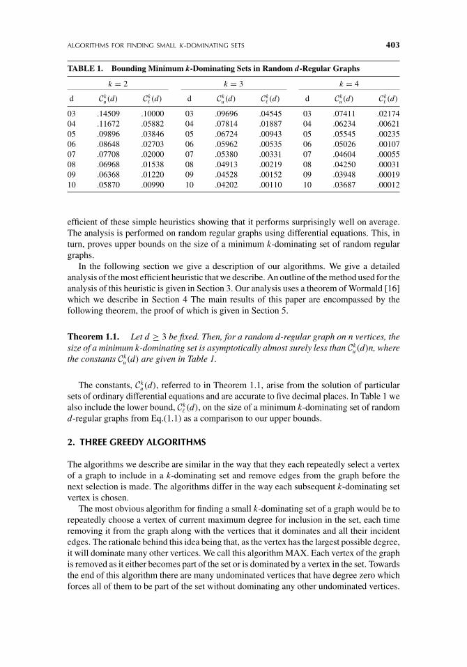
TABLE 1. Bounding Minimum k-Dominating Sets in Random d-Regular Graphs

k = 2 k = 3 k = 4

d Cku(d) Ck

� (d) d Cku(d) Ck

� (d) d Cku(d) Ck

� (d)

03 .14509 .10000 03 .09696 .04545 03 .07411 .0217404 .11672 .05882 04 .07814 .01887 04 .06234 .0062105 .09896 .03846 05 .06724 .00943 05 .05545 .0023506 .08648 .02703 06 .05962 .00535 06 .05026 .0010707 .07708 .02000 07 .05380 .00331 07 .04604 .0005508 .06968 .01538 08 .04913 .00219 08 .04250 .0003109 .06368 .01220 09 .04528 .00152 09 .03948 .0001910 .05870 .00990 10 .04202 .00110 10 .03687 .00012

efficient of these simple heuristics showing that it performs surprisingly well on average.The analysis is performed on random regular graphs using differential equations. This, inturn, proves upper bounds on the size of a minimum k-dominating set of random regulargraphs.

In the following section we give a description of our algorithms. We give a detailedanalysis of the most efficient heuristic that we describe. An outline of the method used for theanalysis of this heuristic is given in Section 3. Our analysis uses a theorem of Wormald [16]which we describe in Section 4 The main results of this paper are encompassed by thefollowing theorem, the proof of which is given in Section 5.

Theorem 1.1. Let d ≥ 3 be fixed. Then, for a random d-regular graph on n vertices, thesize of a minimum k-dominating set is asymptotically almost surely less than Ck

u(d)n, wherethe constants Ck

u(d) are given in Table 1.

The constants, Cku(d), referred to in Theorem 1.1, arise from the solution of particular

sets of ordinary differential equations and are accurate to five decimal places. In Table 1 wealso include the lower bound, Ck

� (d), on the size of a minimum k-dominating set of randomd-regular graphs from Eq.(1.1) as a comparison to our upper bounds.

2. THREE GREEDY ALGORITHMS

The algorithms we describe are similar in the way that they each repeatedly select a vertexof a graph to include in a k-dominating set and remove edges from the graph before thenext selection is made. The algorithms differ in the way each subsequent k-dominating setvertex is chosen.

The most obvious algorithm for finding a small k-dominating set of a graph would be torepeatedly choose a vertex of current maximum degree for inclusion in the set, each timeremoving it from the graph along with the vertices that it dominates and all their incidentedges. The rationale behind this idea being that, as the vertex has the largest possible degree,it will dominate many other vertices. We call this algorithm MAX. Each vertex of the graphis removed as it either becomes part of the set or is dominated by a vertex in the set. Towardsthe end of this algorithm there are many undominated vertices that have degree zero whichforces all of them to be part of the set without dominating any other undominated vertices.


This is one of the reasons for its poor performance. We do not give a detailed analysis ofthis algorithm here as we introduce another (more efficient) algorithm later.

The current best known algorithm for finding a small dominating set of regular graphs [6]is based on choosing vertices from those of current minimum degree. Dominating setvertices are chosen from vertices with current maximum degree among the neighbors ofvertices with current minimum degree. This gives rise to an algorithm for k-dominatingsets which we call MIN. For small values of d and k, this algorithm gives an improvedperformance on that of MAX. However, as d and k become larger, it has a worse average-caseperformance.

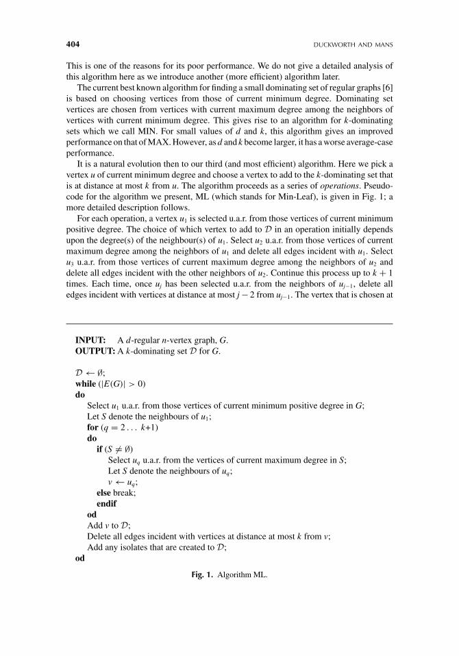
It is a natural evolution then to our third (and most efficient) algorithm. Here we pick avertex u of current minimum degree and choose a vertex to add to the k-dominating set thatis at distance at most k from u. The algorithm proceeds as a series of operations. Pseudo-code for the algorithm we present, ML (which stands for Min-Leaf), is given in Fig. 1; amore detailed description follows.

For each operation, a vertex u1 is selected u.a.r. from those vertices of current minimumpositive degree. The choice of which vertex to add to D in an operation initially dependsupon the degree(s) of the neighbour(s) of u1. Select u2 u.a.r. from those vertices of currentmaximum degree among the neighbors of u1 and delete all edges incident with u1. Selectu3 u.a.r. from those vertices of current maximum degree among the neighbors of u2 anddelete all edges incident with the other neighbors of u2. Continue this process up to k + 1times. Each time, once uj has been selected u.a.r. from the neighbors of uj−1, delete alledges incident with vertices at distance at most j − 2 from uj−1. The vertex that is chosen at

INPUT: A d-regular n-vertex graph, G.OUTPUT: A k-dominating set D for G.

D ← ∅;while (|E(G)| > 0)do

Select u1 u.a.r. from those vertices of current minimum positive degree in G;Let S denote the neighbours of u1;for (q = 2 . . . k+1)do

if (S �= ∅)Select uq u.a.r. from the vertices of current maximum degree in S;Let S denote the neighbours of uq;v ← uq;

else break;endif

odAdd v to D;Delete all edges incident with vertices at distance at most k from v;Add any isolates that are created to D;

od

Fig. 1. Algorithm ML.


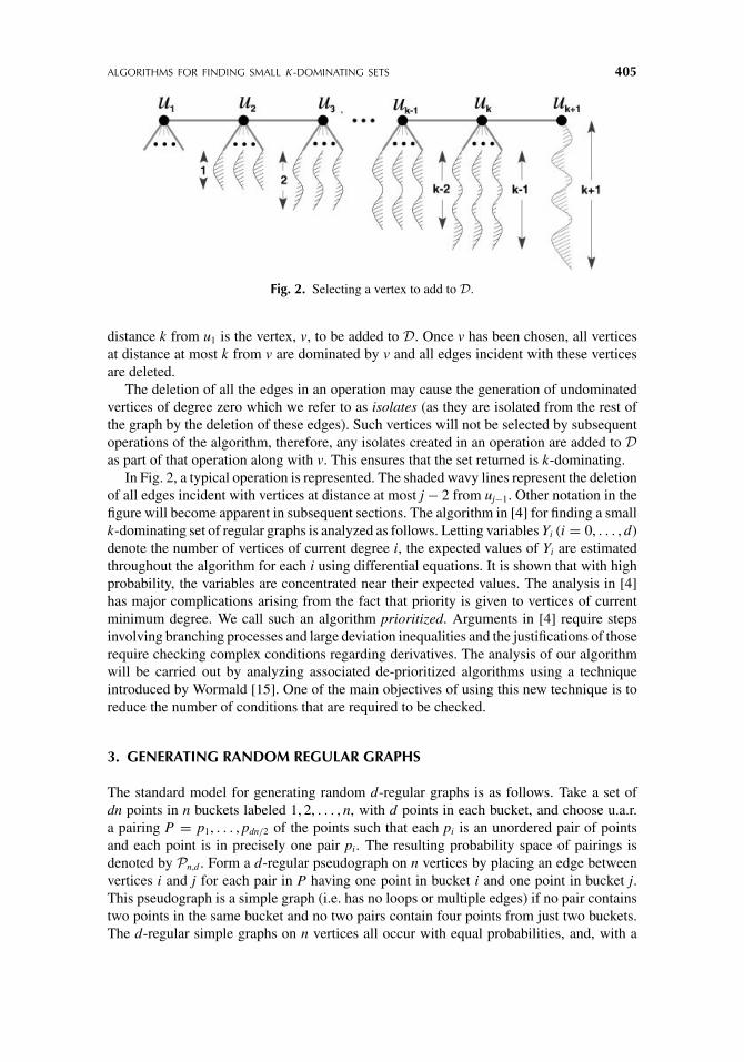
Fig. 2. Selecting a vertex to add to D.

distance k from u1 is the vertex, v, to be added to D. Once v has been chosen, all verticesat distance at most k from v are dominated by v and all edges incident with these verticesare deleted.

The deletion of all the edges in an operation may cause the generation of undominatedvertices of degree zero which we refer to as isolates (as they are isolated from the rest ofthe graph by the deletion of these edges). Such vertices will not be selected by subsequentoperations of the algorithm, therefore, any isolates created in an operation are added to Das part of that operation along with v. This ensures that the set returned is k-dominating.

In Fig. 2, a typical operation is represented. The shaded wavy lines represent the deletionof all edges incident with vertices at distance at most j − 2 from uj−1. Other notation in thefigure will become apparent in subsequent sections. The algorithm in [4] for finding a smallk-dominating set of regular graphs is analyzed as follows. Letting variables Yi (i = 0, . . . , d)denote the number of vertices of current degree i, the expected values of Yi are estimatedthroughout the algorithm for each i using differential equations. It is shown that with highprobability, the variables are concentrated near their expected values. The analysis in [4]has major complications arising from the fact that priority is given to vertices of currentminimum degree. We call such an algorithm prioritized. Arguments in [4] require stepsinvolving branching processes and large deviation inequalities and the justifications of thoserequire checking complex conditions regarding derivatives. The analysis of our algorithmwill be carried out by analyzing associated de-prioritized algorithms using a techniqueintroduced by Wormald [15]. One of the main objectives of using this new technique is toreduce the number of conditions that are required to be checked.

3. GENERATING RANDOM REGULAR GRAPHS

The standard model for generating random d-regular graphs is as follows. Take a set ofdn points in n buckets labeled 1, 2, . . . , n, with d points in each bucket, and choose u.a.r.a pairing P = p1, . . . , pdn/2 of the points such that each pi is an unordered pair of pointsand each point is in precisely one pair pi. The resulting probability space of pairings isdenoted by Pn,d . Form a d-regular pseudograph on n vertices by placing an edge betweenvertices i and j for each pair in P having one point in bucket i and one point in bucket j.This pseudograph is a simple graph (i.e. has no loops or multiple edges) if no pair containstwo points in the same bucket and no two pairs contain four points from just two buckets.The d-regular simple graphs on n vertices all occur with equal probabilities, and, with a


probability that is asymptotic to e(1−d2)/4, the pseudograph corresponding to the randompairing in Pn,d is simple. It follows that, in order to prove that a property is a.a.s. true of auniformly distributed random d-regular (simple) graph, it is enough to prove that it is a.a.s.true of the pseudograph corresponding to a random pairing.

As in [6, 15], we redefine this model slightly by specifying that the pairs are chosensequentially. The first point in a random pair may be selected using any rule whatsoever,as long as the second point in that random pair is chosen u.a.r. from all the remaining free(unpaired) points. This preserves the uniform distribution of the final pairing (see [16, p. 19]or Bollobás [1]).

When a pair has been determined in the sequential process, we say that it has beenexposed. By exposing pairs in the order which an algorithm requests their existence, thegeneration of the random pairing may be combined with the algorithm (as in [15]). Thismay be explained alternatively as follows. Suppose that the pairing generation consistsof a sequence of operations OP0, OP1, . . ., each exposing at least one of the pairs. Analgorithm, which examines edges in the same order as that for the pairing generation, maybe incorporated into the pairing process by extending the definition of the operations tocover all the tasks of the algorithm.

The algorithm being referred to acts upon the final (pseudo)graph of the generationprocess. It is convenient to regard the operations of that algorithm as sequentially deletingthe exposed pairs (edges) from this graph. For this reason, we refer to it as the deletionalgorithm which is being carried out, to distinguish it from the pairing generation. At eachpoint, the graph in the deletion algorithm contains all the edges of the final graph whichhave not yet been exposed. In this way, the prioritized algorithm may be described in termsof operations incorporated into the pairing generation.

A set D and the pairing are initially empty. Then, for an integer t ≥ 0, the operationOP t randomly selects a bucket u with the current maximum degree, the degree of a bucketbeing the number of points in that bucket which are in exposed pairs. (This is equivalentto a vertex of current minimum degree in the graph in the deletion algorithm.) It thenexposes all remaining edges incident with the vertex corresponding to the bucket u. Thisallows us to determine the degrees of the vertices corresponding to the buckets incidentwith these exposed edges. Further edges may then be exposed, and a vertex v may thenbe chosen to be part of D. The reasons why there will always be a vertex at distance kfrom u to add to D (a.a.s.) are not obvious but arise from our analysis. Any other bucketsat distance k + 1 from u that attain degree d are also added to D. These correspond toisolates.

4. ANALYSIS METHOD

In order to approximate the performance of our prioritized algorithm, we analyze associatedde-prioritized algorithms using a result of Wormald [16, Theorem 1]. These algorithms avoidprioritizing by using a randomized mixture of operations. The particular mixture used forany step is prescribed in advance but changes over the course of the algorithm in order toapproximate the prioritized algorithm.

In order to apply [16, Theorem 1] we are required to derive equations that represent theexpected changes in variables that describe the state of the algorithm during its execution.From these equations we develop associated differential equations, the solution of whichapproximate the size of the set of interest at the end of some randomized algorithm. We


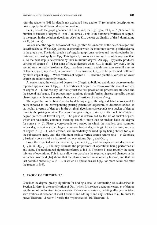
refer the reader to [16] for details not explained here and to [6] for another description onhow to apply the differential equation method.

Let Gt denote the graph generated at time t, and, for 0 ≤ i ≤ d, let Yi = Yi(t) denote thenumber of buckets of degree d − i in Gt (at time t). This is the number of vertices of degree iin the graph in the deletion algorithm. Also let Yd+1 denote cardinality of the k-dominatingset Dt (at time t).

We consider the typical behavior of the algorithm ML in terms of the deletion algorithmdescribed above. We let Opw denote an operation when the minimum current positive degreein the graph is w. The initial graph is a d-regular graph on n vertices and therefore, in the firstinstance, we must apply an Opd . This typically produces some vertices of degree less thand, so the next step is determined by their minimum degree. An Opd−1 typically producesvertices of degree d − 1 but none of lower degrees when Yd−1 is small (say o(n)), so thesecond step normally involves an Opd−1, as does the next, and this remains so until a vertexof lower degree, say d − 2, is produced. This causes an Opd−2 to be performed, followedby more steps of Opd−1. When vertices of degree d − 1 become plentiful, vertices of lowerdegree are more commonly created.

At some stage, the vertices of degree d − 2 begin to build up and do not decrease underrepeated applications of Opd−2. Then vertices of degree d − 2 take over the role of verticesof degree d − 1, and we say informally that the first phase of the process has finished andthe second has begun. The process may continue through further phases; typically, the gthphase begins with an increasing abundance of vertices of degree d − g.

The algorithm in Section 2 works by deleting edges; the edges deleted correspond topairs exposed in the corresponding pairing generation algorithm as described above. Inparticular, a vertex of degree i in the original algorithm corresponds to a bucket of degreed − i in the pairing version. The algorithm gives higher priority to the buckets of highestdegree (vertices of lowest degree). The phase is determined by the set of bucket degreeswhich are reasonably common (meaning, roughly, more than cn buckets have that degreefor some c > 0). Phase g corresponds to a period in which the smallest such commonvertex degree is d − g (i.e., largest common bucket degree is g). At such a time, verticesof degree d − g − 1, when created, will immediately be used up, by being chosen for u1 inthe subsequent steps, until the minimum positive vertex degree returns to d − g. So phaseg basically consists of a mixture of two operations: Opd−g and Opd−g−1.

From the expected net increase in Yg+1 in an Opd−g and the expected net decrease inYg+1 in an Opd−g−1, one may estimate the proportions of operations being performed atany stage. The randomized algorithm referred to in [16, Theorem 1] uses roughly the samemixture of operations. This in turn allows us calculate the required expected changes in thevariables. Wormald [16] shows that the phases proceed in an orderly fashion, and that thelast possible phase is g = d − 1, in which all operations are Op1. For more detail, we referthe reader to [16].

5. PROOF OF THEOREM 1.1

Consider the degree-greedy algorithm for finding a small k-dominating set as described inSection 2. Here, in the specification of Opw (which first selects a random vertex, u, of degreew), the set of randomized tasks consists of choosing a vertex v, deleting all edges incidentwith vertices at distance at most k from v and adding v and any isolates to D. In order toprove Theorem 1.1 we will verify the hypotheses of [16, Theorem 1].


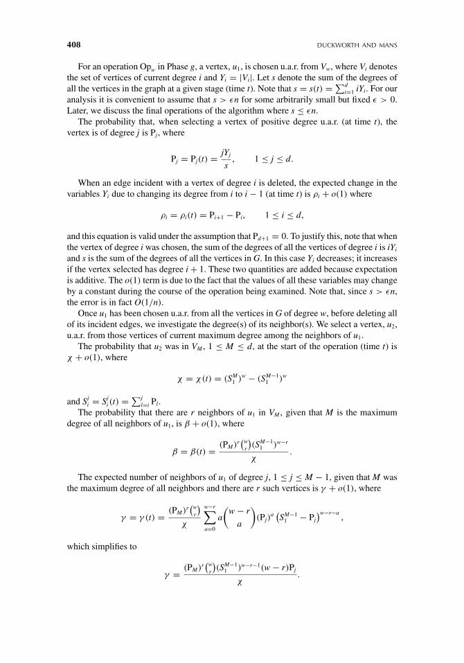
For an operation Opw in Phase g, a vertex, u1, is chosen u.a.r. from Vw, where Vi denotesthe set of vertices of current degree i and Yi = |Vi|. Let s denote the sum of the degrees ofall the vertices in the graph at a given stage (time t). Note that s = s(t) = ∑d

i=1 iYi. For ouranalysis it is convenient to assume that s > εn for some arbitrarily small but fixed ε > 0.Later, we discuss the final operations of the algorithm where s ≤ εn.

The probability that, when selecting a vertex of positive degree u.a.r. (at time t), thevertex is of degree j is Pj, where

Pj = Pj(t) = jYj

s, 1 ≤ j ≤ d.

When an edge incident with a vertex of degree i is deleted, the expected change in thevariables Yi due to changing its degree from i to i − 1 (at time t) is ρi + o(1) where

ρi = ρi(t) = Pi+1 − Pi, 1 ≤ i ≤ d,

and this equation is valid under the assumption that Pd+1 = 0. To justify this, note that whenthe vertex of degree i was chosen, the sum of the degrees of all the vertices of degree i is iYi

and s is the sum of the degrees of all the vertices in G. In this case Yi decreases; it increasesif the vertex selected has degree i + 1. These two quantities are added because expectationis additive. The o(1) term is due to the fact that the values of all these variables may changeby a constant during the course of the operation being examined. Note that, since s > εn,the error is in fact O(1/n).

Once u1 has been chosen u.a.r. from all the vertices in G of degree w, before deleting allof its incident edges, we investigate the degree(s) of its neighbor(s). We select a vertex, u2,u.a.r. from those vertices of current maximum degree among the neighbors of u1.

The probability that u2 was in VM , 1 ≤ M ≤ d, at the start of the operation (time t) isχ + o(1), where

χ = χ(t) = (SM1 )w − (SM−1

1 )w

and Sji = Sj

i(t) = ∑jl=i Pl.

The probability that there are r neighbors of u1 in VM , given that M is the maximumdegree of all neighbors of u1, is β + o(1), where

β = β(t) = (PM)r(w

r

)(SM−1

1 )w−r

χ.

The expected number of neighbors of u1 of degree j, 1 ≤ j ≤ M − 1, given that M wasthe maximum degree of all neighbors and there are r such vertices is γ + o(1), where

γ = γ (t) = (PM)r(w

r

)χ

w−r∑a=0

a

(w − r

a

)(Pj)

a(SM−1

1 − Pj

)w−r−a,

which simplifies to

γ = (PM)r(w

r

)(SM−1

1 )w−r−1(w − r)Pj

χ.


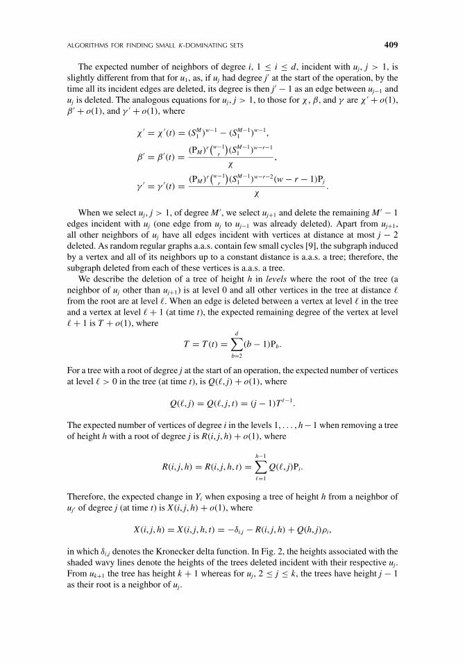
The expected number of neighbors of degree i, 1 ≤ i ≤ d, incident with uj, j > 1, isslightly different from that for u1, as, if uj had degree j′ at the start of the operation, by thetime all its incident edges are deleted, its degree is then j′ − 1 as an edge between uj−1 anduj is deleted. The analogous equations for uj, j > 1, to those for χ , β, and γ are χ ′ + o(1),β ′ + o(1), and γ ′ + o(1), where

χ ′ = χ ′(t) = (SM1 )w−1 − (SM−1

1 )w−1,

β ′ = β ′(t) = (PM)r(w−1

r

)(SM−1

1 )w−r−1

χ,

γ ′ = γ ′(t) = (PM)r(w−1

r

)(SM−1

1 )w−r−2(w − r − 1)Pj

χ.

When we select uj, j > 1, of degree M ′, we select uj+1 and delete the remaining M ′ − 1edges incident with uj (one edge from uj to uj−1 was already deleted). Apart from uj+1,all other neighbors of uj have all edges incident with vertices at distance at most j − 2deleted. As random regular graphs a.a.s. contain few small cycles [9], the subgraph inducedby a vertex and all of its neighbors up to a constant distance is a.a.s. a tree; therefore, thesubgraph deleted from each of these vertices is a.a.s. a tree.

We describe the deletion of a tree of height h in levels where the root of the tree (aneighbor of uj other than uj+1) is at level 0 and all other vertices in the tree at distance �

from the root are at level �. When an edge is deleted between a vertex at level � in the treeand a vertex at level � + 1 (at time t), the expected remaining degree of the vertex at level� + 1 is T + o(1), where

T = T(t) =d∑

b=2

(b − 1)Pb.

For a tree with a root of degree j at the start of an operation, the expected number of verticesat level � > 0 in the tree (at time t), is Q(�, j) + o(1), where

Q(�, j) = Q(�, j, t) = (j − 1)T �−1.

The expected number of vertices of degree i in the levels 1, . . . , h − 1 when removing a treeof height h with a root of degree j is R(i, j, h) + o(1), where

R(i, j, h) = R(i, j, h, t) =h−1∑�=1

Q(�, j)Pi.

Therefore, the expected change in Yi when exposing a tree of height h from a neighbor ofuj′ of degree j (at time t) is X(i, j, h) + o(1), where

X(i, j, h) = X(i, j, h, t) = −δi,j − R(i, j, h) + Q(h, j)ρi,

in which δi,j denotes the Kronecker delta function. In Fig. 2, the heights associated with theshaded wavy lines denote the heights of the trees deleted incident with their respective uj.From uk+1 the tree has height k + 1 whereas for uj, 2 ≤ j ≤ k, the trees have height j − 1as their root is a neighbor of uj.


The expected change in Yi when performing an operation Opw in Phase g is φi,w,k +o(1) =φi,w,k,t + o(1), where φi,w,0 is given by

X(i, w, k + 1), (5.1)

φi,w,k is given by

−δi,w +d∑

M=1

χ [φi,M,k−1 +w∑

r=1

β(r − 1)(δi,M−1 − δi,M) +M−1∑j=1

γ (δi,j−1 − δi,j)] (5.2)

and for 0 < κ < k, φi,w,κ is given by

−δi,w +d∑

M=1

χ ′[φi,M,κ−1 +w−1∑r=1

β ′(r − 1)X(i, M, k − κ) +M−1∑j=1

γ ′X(i, j, k − κ)]. (5.3)

It follows that Eqs. (5.1)–(5.3) are also valid to compute the expected increase in thesize of the k-dominating set for an Opw when i = d + 1 with φd+1,w,k defined as 1 + φ0,w,k ,since, in each Opw, at least one vertex is added to the k-dominating set D and the expectednumber of isolates is φ0,w,k as defined in Eqs. (5.1)–(5.3).

Equations (5.1)–(5.3) form the basis of a set of differential equations. We refer thereader to [16, Theorem 1] for more detail and for motivation for the following definitions.Put Y(t) = (Y1(t), . . . , Yd+1(t)) and let y(x) denote (y1(x), . . . , yd+1(x)), where

x = t

n, y(x) = Y(t)

n. (5.4)

Given functions φi,w,k (x, y), define

αg(x, y) = φw,w−1,k (x, y) ,

τg(x, y) = −φw−1,w−1,k (x, y) .(5.5)

We will consider the equations

dyi

dx= F (x, y, i, k, g) , where (5.6)

F (x, y, i, k, g) =

τg

τg + αgφi,w,k (x, y) + αg

τg + αgφi,w−1,k (x, y) (if g ≤ d − 2),

φi,1,k (x, y) (if g = d − 1),(5.7)

and work with the parameters of φi,w,k in the domain

Rε = {(x, y) : 0 ≤ x ≤ d, 0 ≤ yi ≤ d for 1 ≤ i ≤ d + 1, yd ≥ ε} (5.8)

for some prechosen value of ε > 0.It remains to verify the hypotheses of [16, Theorem 1]. Hypothesis (i) of [16, Theorem 1]

is immediate since in any operation only a constant number of edges are deleted and abounded number of vertices are added to D. The functions φi,w,k satisfy hypothesis (ii)of [16, Theorem 1] because from Eqs. (5.1)–(5.3), their (possible) singularities satisfy


s = 0, which lies outside Rε since in Rε , s ≥ yd ≥ ε. Hypothesis (iii) of [16, Theorem 1]follows again from Equations (5.1)–(5.3) using s ≥ yd ≥ ε and the boundedness of Rε .

Thus, defining Yd(0) = n and Yi(0) = 0 for i �= d, we may solve 5.6 numerically tofind the end of the process, verifying the necessary conditions from [16, Theorem 1] at theappropriate points of the computation.

It turns out that these hold for each d and k which was treated numerically in [4], andthat in each case the final phase of the process is m = d − 1, for sufficiently small ε > 0.For such ε, the value of yd+1 at the end of Phase m may be computed numerically (the resultis shown as the constants Ck

u(d) in Table 1), and then by Theorem [16, Theorem 1], this isthe asymptotic value of the size of the k-dominating set D (scaled by n) at the end of somerandomized algorithm.

This completes the proof of Theorem 1.1.

REFERENCES

[1] B. Bollobás, Random graphs, Academic [Harcourt Brace Jovanovich], London, 1985.

[2] G. J. Chang and G. L. Nemhauser, The k-domination and k-stability problems on graphs,Technical Report TR-540, School of Operations Research and Industrial Engineering, CornellUniversity, Ithaca, NY, 1982.

[3] R. Diestel, Graph theory, Springer, New York, 2000.

[4] W. Duckworth and B. Mans, “Small k-dominating sets of regular graphs,” Proceedings of theSixth International Workshop on Randomization and Approximation Techniques in ComputerScience, Eds., J. D. P. Rolim and S. P. Vadhan, Lecture Notes in Computer Science, 2483,126–138. Springer, New York, 2002.

[5] W. Duckworth and N. C. Wormald, Minimum independent dominating sets of random cubicgraphs, Random Structures Algorithms, 21(2) (2002), 147–161.

[6] W. Duckworth and N. C. Wormald, On the independent domination number of random regulargraphs, Combin Probab Comput, in press.

[7] O. Favaron, T. W. Haynes, and P. J. Slater, Distance-k independent domination sequences, JCombin Math Combin Comput, 33 (2000), 225–237.

[8] T. W. Haynes, S. T. Hedetniemi, and P. J. Slater, Eds., Domination in graphs: Advanced topics.,volume 209 of Monographs and Textbooks in Pure and Applied Mathematics, Marcel Dekker,New York, 1998.

[9] S. Janson, T. Łuczak, and A. Rucinski, Random graphs, Wiley-Interscience Series in DiscreteMathematics and Optimization, Wiley-Interscience, New York, 2000.

[10] D. S. Johnson, Approximation algorithms for combinatorial problems, Proc Fifth Annual ACMSymp Theory of Computing, Austin, TX, 1973. J Comput System Sci 9 (1974), 256–278.

[11] S. Kutten and D. Peleg, Fast distributed construction of small k-dominating sets andapplications, J Algorithms 28(1) 1998, 40–66.

[12] C. H. Papadimitriou and M. Yannakakis, Optimization, approximation and complexity classes,J Comput System Sci 43(3) 1991, 425–440.

[13] R. Raz and S. Safra, A sub-constant error-probability low-degree test and a sub-constant error-probability PCP characterization of NP, Proc Twenty-Ninth Annual ACM Symp Theory ofComputing El Paso, TX, ACM, New York, 1999, pp. 475–484 (electronic).

[14] R. W. Robinson and N. C. Wormald, Almost all regular graphs are Hamiltonian, RandomStructures Algorithms 5(2) (1994), 363–374.


[15] N. C. Wormald, “The differential equation method for random graph processes and greedyalgorithms,” Lectures on approximation and randomized algorithms, Eds., M. Karonski andH. J. Prömel, 73–155. PWN, Warsaw, 1999.

[16] N. C. Wormald, Analysis of greedy algorithms on graphs with bounded degrees, Discrete Math,273 (2003), 235–260.

[17] M. Zito, “Greedy algorithms for minimisation problems in random regular graphs,” Proceedingsof the Ninth Annual European Symposium on Algorithms, Eds., F. Meyer auf der Heide, LectureNotes in Computer Science 2161, 524–536. Springer, New York, 2001.

Documents

Randomized greedy algorithms for finding small k-dominating sets of regular graphs