Embed Size (px)
Citation preview
Last revised 9:55 a.m. August 17, 2015
Rank assignment and the Robinson-Schensted-Knuth algorit hm
Bill Casselman
University of British [email protected]
The algorithm of Robinson, Schensted, and Knuth establishes a bijection of the symmetric group Sn withpairs of Young tableaux of size n and the same shape. There is already a huge literature on this topic, but
it seems to me that the RSK algorithm is familiar to us only through habituation, not through any goodunderstanding as to how one might have come across it to begin with. That is what I hope to supply here.
What is new is that I use the problem of rank assignment in a partially ordered set as motivation for the
algorithm. This has the advantage of leading to a new and perhaps more transparent proof of its symmetry.Also apparently somewhat new here is how I treat some aspects of Knuth equivalence in the last section.
Nowadays, the RSK algorithm is of interest in many fields of mathematics, but my own interest is almostexclusively in its relationship to theW cells of [KazhdanLusztig:1979] (for this, see [GarsiaMcLarnan:1988],
[Ariki:2000], and [Du:2005]). I’ll discuss this elsewhere, since it is not elementary. Another application of
great interest in representation theory that I’ll skip, albeit reluctantly, can be found in [Steinberg:1988].
I begin with the problem that motivated Schensted’s original paper, that of finding subsequences of maximal
length in an arbitrary sequence of distinct integers. But a natural approach to Schensted’s algorithm comesfrom something also quite natural, the problem of assigning ranks in a partially ordered set. That is where I
shall actually start. In this I am expanding the treatment in §4 of [Knuth:1970] (see also §5.1.4 of [Knuth:1975]).
I wish to offer my great gratitude to Darij Grinberg for reading earlier versions of this essay thoroughly,
pointing out several places where clarity was lacking and—to my embarrassment and horror—statements
incorrect.
Contents
I. Symmetry1. Computing rank in a partially ordered set
2. Schensted’s problem3. Schensted’s solution
4. Schensted’s extended algorithm
5. Tableaux6. Going backwards
7. Delayed pair processing
8. Symmetry9. Appendix. Python code
II. Cells10. Descents and tableaux
11. Knuth equivalence
12. More about Knuth equivalenceIII. References
Part I. Symmetry
RobinsonSchensted 2
1. Computing rank in a partially ordered set
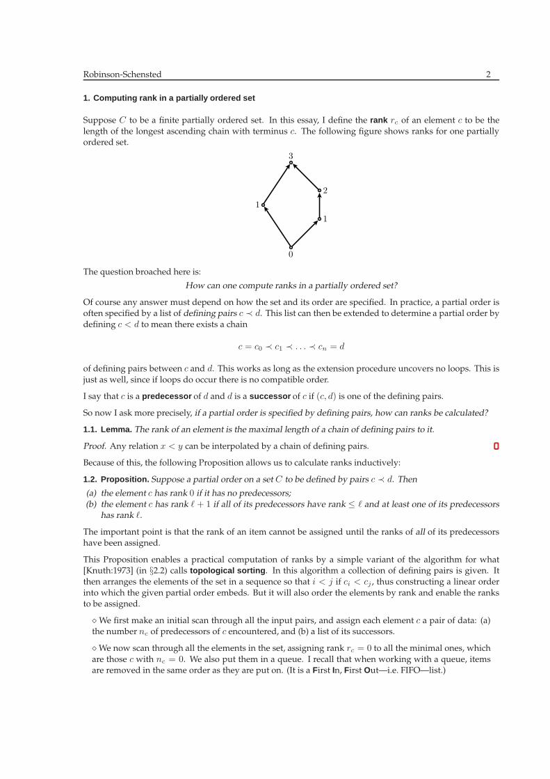
Suppose C to be a finite partially ordered set. In this essay, I define the rank rc of an element c to be the
length of the longest ascending chain with terminus c. The following figure shows ranks for one partiallyordered set.
0
1
2
3
1
The question broached here is:
How can one compute ranks in a partially ordered set?
Of course any answer must depend on how the set and its order are specified. In practice, a partial order isoften specified by a list of defining pairs c ≺ d. This list can then be extended to determine a partial order by
defining c < d to mean there exists a chain
c = c0 ≺ c1 ≺ . . . ≺ cn = d
of defining pairs between c and d. This works as long as the extension procedure uncovers no loops. This is
just as well, since if loops do occur there is no compatible order.
I say that c is a predecessor of d and d is a successor of c if (c, d) is one of the defining pairs.
So now I ask more precisely, if a partial order is specified by defining pairs, how can ranks be calculated?
1.1. Lemma. The rank of an element is the maximal length of a chain of defining pairs to it.
Proof. Any relation x < y can be interpolated by a chain of defining pairs.
Because of this, the following Proposition allows us to calculate ranks inductively:
1.2. Proposition. Suppose a partial order on a set C to be defined by pairs c ≺ d. Then
(a) the element c has rank 0 if it has no predecessors;(b) the element c has rank ℓ + 1 if all of its predecessors have rank ≤ ℓ and at least one of its predecessors
has rank ℓ.
The important point is that the rank of an item cannot be assigned until the ranks of all of its predecessorshave been assigned.
This Proposition enables a practical computation of ranks by a simple variant of the algorithm for what[Knuth:1973] (in §2.2) calls topological sorting . In this algorithm a collection of defining pairs is given. It
then arranges the elements of the set in a sequence so that i < j if ci < cj , thus constructing a linear order
into which the given partial order embeds. But it will also order the elements by rank and enable the ranksto be assigned.
⋄We first make an initial scan through all the input pairs, and assign each element c a pair of data: (a)the number nc of predecessors of c encountered, and (b) a list of its successors.
⋄We now scan through all the elements in the set, assigning rank rc = 0 to all the minimal ones, which
are those c with nc = 0. We also put them in a queue. I recall that when working with a queue, itemsare removed in the same order as they are put on. (It is a First In, First Out—i.e. FIFO—list.)

RobinsonSchensted 3
⋄We initialize the array that will eventually hold all the elements in linear order, but which starts outempty.
⋄ As long as the queue isn’t empty, we pop an item c off it and put it at the end of the sorted list weare building. Then we run through the list of the successors of c, decrementing the predecessor count
of each. If d is one of these successors and if nd becomes 0, then d is minimal in the current unranked
group, we set rd = rc + 1, and we put it in the queue. Loop to look at the queue again.
An item is put on the queue before any of its successors, so (precisely because it is a queue) it is removed
from it before them, and it is therefore also put on the sorted list before any of them. This ensures that thelinear order implicit in the list is compatible with the original partial order.
At the end, we have both assigned ranks and listed all the elements of C in an order compatible with rank.
This very basic algorithm is embedded in many standard computer programs, for example in computing
dependencies in the UNIX utility make. It is not hard to modify it slightly so as to find a chain of maximal
length—whenwe assign rd in the procedure above, define the special predecessor of d to be c. At the end, thelast item in the list will havemaximal rank, and going through its special predecessor, the special predecessor
of this in turn, etc. builds a maximal chain.
2. Schensted’s problem
The procedure laid out in the previous section will find ranks in any partially ordered set, but if the order is
not given in the form of pairs a ≺ b we’d have to first find such data. This may not be terribly easy to do. We
shall instead look at a very special class of partially ordered sets, and see for these an efficient algorithm tofind ranks in it. This algorithm is primarily due to C. E. Schensted, although something prior was found by
G. de B. Robinson. (The history is recounted on p. 60 of [Knuth:1975].)
The original problem of Schensted is to find the maximum length of an increasing subsequence of a given
sequence of distinct integers. For example, consider (6, 3, 1, 7, 2, 5, 8, 4). There is a very simple, if somewhat
inefficient, way to solve the problem, basically reducing it to the procedure described in the previous section.First scan the array to make a list of all increasing pairs, then rescan to make a list of increasing triples that
extend these, and so on. For this array, the list of pairs is
(6, 7), (6, 8), (3, 7), (3, 5), (3, 8), (3, 4), (1, 7), (1, 2),
(1, 5), (1, 8), (1, 4), (7, 8), (2, 5), (2, 8), (2, 4), (5, 8) .
The set of ordered triples is then
(6, 7, 8), (3, 7, 8), (3, 5, 8), (1, 7, 8), (1, 2, 5), (1, 2, 8), (1, 2, 4), (1, 5, 8), (2, 5, 8) .
Of these, exactly one extends to a sequence of length four: (1, 2, 5, 8), which extends no further.
The extra steps from pairs to triples, etc. is actually closely related to the process we went through in §1. Thelist of increasing pairs is a set of defining pairs for a partial order on a certain set. It can be interpreted as alist of relations
6 ≺ 7, 6 ≺ 8, 3 ≺ 7, . . .
We can then assemble the pairs (1, 2), (2, 5) (5, 8) to get our longest sequence. This notation is not ideal,however. The relation 6 ≺ 7 does not mean just that 6 < 7, but that 6 < 7 and 6 occurs before 7 in the given
sequence. This suggests that we make the original list (pi) into a new sequence of pairs (i, pi). The order
imposed on this is(i, p) ≤ (i∗, p∗) when i ≤ i∗ and p ≤ p∗ .
What is special about this partial order is that the initial sequence is ordered according to the initial entry of
each pair.

RobinsonSchensted 4
2.1. Lemma. The map taking pi1 < pi2 < . . . to (i1, pi1) < (i2, pi2) < . . . is a bijection between increasingsubsequences in the original sequence and chains in the new ordered set of pairs.
As a consequence, the length of the longest subsequence is equal to the maximum rank assigned.
Being given the sequence of the pi means that in effect we are starting with a topological sort of the pairs
(i, pi). For example, for the sequence (6, 3, 1, 7, 2, 5, 8, 4)we get the pairs
(1, 6), (2, 3), (3, 1), (4, 7), (5, 2), (6, 5), (7, 8), (8, 4) .
The additional initial coordinate will play a role later on, but can be forgotten for a while.
With this approach, the hardest work goes into finding all the defining pairs. The amount of effort it takes
to do this is basically proportional to the square of the size of the list. This is not an outrageous amount of
work, but difficult enough, and impossible by hand on a large list, for example this one:
(41, 93, 31, 73, 98, 29, 12, 54, 24, 0, 52, 78, 87, 55, 25, 81, 76,
91, 51, 7, 39, 92, 65, 40, 45, 5, 1, 20, 84, 99, 27, 32, 13, 8, 2,
61, 19, 9, 74, 60, 66, 79, 47, 86, 30, 3, 85, 42, 89, 43, 70, 17,
6, 63, 28, 11, 34, 75, 22, 64, 59, 16, 48, 15, 90, 80, 69, 67,
35, 72, 50, 14, 33, 53, 10, 38, 94, 18, 58, 46, 49, 88, 68, 21,
62, 44, 97, 82, 37, 83, 95, 4, 56, 57, 77, 23, 96, 26, 36, 71) ,
which we shall be able to handle later without difficulty.
We can now assign ranks according to the following slightly more direct process:
⋄ The first item p1 has no predecessors and consequently gets rank 0;⋄ the item pi (i > 1) gets rank h if
(a) there is a prior item pj < pi (‘prior’ means j < i) of rank h− 1 and
(b) there are no prior items pj < pi of rank ≥ h.
That is to say, we assign ranks as we read the sequence pi, instead of finding first all the increasing pairs.
When assigning a rank to pn the obvious thing to do is scan back through the ranks ri of the prior pi (i.e. withi < n) looking to verify (a) and (b). For example, look again at (6, 3, 1, 7, 2, 5, 8, 4). We start with
pi 6 3 1 7 2 5 8 4
ri 0
We have p2 = 3, and since p1 = 6 > p2 the rank of this new item is also 0.
pi 6 3 1 7 2 5 8 4ri 0 0
Similarly r3 = 0. What about r4? Since p4 = 7 > p1 = 6, p2 = 2, p3 = 1, all of which have rank 0, we haver4 = 1
pi 6 3 1 7 2 5 8 4
ri 0 0 0 1
Usw. Here all the ranks have been assigned:
pi 6 3 1 7 2 5 8 4Rank 0 0 0 1 1 2 3 2
This process is still not ideal, because the amount of time it takes still seems to be roughly proportional ton2. Some version of this procedure works for any partially ordered set, but there is something special about
the one at hand that allows us to do better. As often in programs, we can gain time by using more space
to record progress. In this case, however, we shall eventually be able to reclaim the space, only temporarilylost, at no cost in time.
RobinsonSchensted 5
3. Schensted’s solution
There is one way to modify the procedure so as to work a bit more efficiently. It is not necessary to scan
through all the prior pi when assigning the rank of pj . We shall maintain lists of the objects of various ranks,and in order of rank. Then in order to assign the rank of pj , we have only to scan backwards though these
lists, starting with the highest rank assigned so far, until we find one pi with i < j and pi < pj . At this point,
we have located an item prior to pj with maximum rank. We set rj = ri + 1, and add pj to the list of itemsof rank rj .
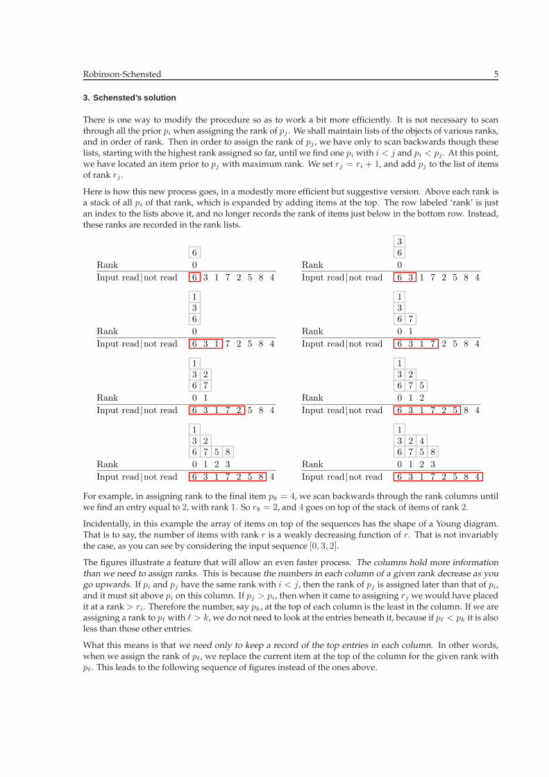
Here is how this new process goes, in a modestly more efficient but suggestive version. Above each rank isa stack of all pi of that rank, which is expanded by adding items at the top. The row labeled ‘rank’ is just
an index to the lists above it, and no longer records the rank of items just below in the bottom row. Instead,
these ranks are recorded in the rank lists.
Input read |not read
Rank 0
6 3 1 7 2 5 8 4
6
Input read |not read
Rank 0
6 3 1 7 2 5 8 4
63
Input read |not read
Rank 0
6 3 1 7 2 5 8 4
631
Input read |not read
Rank 0 1
6 3 1 7 2 5 8 4
631
7
Input read |not read
Rank 0 1
6 3 1 7 2 5 8 4
631
72
Input read |not read
Rank 0 1 2
6 3 1 7 2 5 8 4
631
72
5
Input read |not read
Rank 0 1 2 3
6 3 1 7 2 5 8 4
631
72
5 8
Input read |not read
Rank 0 1 2 3
6 3 1 7 2 5 8 4
631
72
5 84
For example, in assigning rank to the final item p8 = 4, we scan backwards through the rank columns until
we find an entry equal to 2, with rank 1. So r8 = 2, and 4 goes on top of the stack of items of rank 2.
Incidentally, in this example the array of items on top of the sequences has the shape of a Young diagram.
That is to say, the number of items with rank r is a weakly decreasing function of r. That is not invariablythe case, as you can see by considering the input sequence [0, 3, 2].
The figures illustrate a feature that will allow an even faster process. The columns hold more informationthan we need to assign ranks. This is because the numbers in each column of a given rank decrease as yougo upwards. If pi and pj have the same rank with i < j, then the rank of pj is assigned later than that of pi,
and it must sit above pi on this column. If pj > pi, then when it came to assigning rj we would have placed
it at a rank > ri. Therefore the number, say pk, at the top of each column is the least in the column. If we areassigning a rank to pℓ with ℓ > k, we do not need to look at the entries beneath it, because if pℓ < pk it is also
less than those other entries.
What this means is that we need only to keep a record of the top entries in each column. In other words,
when we assign the rank of pℓ, we replace the current item at the top of the column for the given rank with
pℓ. This leads to the following sequence of figures instead of the ones above.
RobinsonSchensted 6
Input read |not readRank 0 1 2 3
6 3 1 7 2 5 8 4
6
Input read |not readRank 0 1 2 3
6 3 1 7 2 5 8 4
63
Input read |not readRank 0 1 2 3
6 3 1 7 2 5 8 4
631
Input read |not readRank 0 1 2 3
6 3 1 7 2 5 8 4
631 7
Input read |not readRank 0 1 2 3
6 3 1 7 2 5 8 4
631 72
Input read |not readRank 0 1 2 3
6 3 1 7 2 5 8 4
631 72 5
Input read |not readRank 0 1 2 3
6 3 1 7 2 5 8 4
631 72 5 8
Input read |not readRank 0 1 2 3
6 3 1 7 2 5 8 4
631 72 5 84
Now what happens when we read the last item 4? We scan back through the row of boxes, until we get
blocked by the entry 2. At that point we drop 4 into the box just ahead of it, replacing the 5. It is said that the4 bumps or bounces or extrudes the 5. This, finally, is Schensted’s row-insertion process .
There is a minor problem with this method—it no longer records permanently all rank assignments. What itdoes do is record the maximum height attained, which from now on we’ll be satisfied with.
These figures illustrate another feature of this process: The sequence of tops—the numbers in the boxes—area monotonic increasing sequence, read left to right. This can be proved by induction on the number of items
in the sequence to be read.
The sequence of 100 integers written down at the beginning is now entirely feasible. We get the length of a
longest subsequence to be 15, and a subsequence of that length to be
i 9 26 34 45 52 55 71 72 75 79 80 92 93 94 95pi 0 1 2 3 6 11 14 33 38 46 49 56 57 77 96
It is not too difficult to do this by hand, but when programming the Schensted process for large sequencesyou will want to be more efficient. Searching backwards through the row is important theoretically, as we’ll
see later, but the amount of time it takes is roughly proportional to the length of the row. You can do much
better with a binary search to locate where to insert and bounce.
I’ll now lay out the process more completely.
⋄ We start with a sequence of distinct integers pi. I’ll assume that we want merely to say what thelength of the longest increasing subsequence is—actually finding that subsequence would involve an
easy modification that I have already suggested in the first section.
⋄ The process maintains the array that sits at the tops of the stacks of the pi of a given rank. The state at
any moment therefore consists of two arrays—this rank array and the input sequence.
⋄At the start the first is empty and the second is the entire sequence of the pi. In each step, the next input
pk is removed from input and the rank array is modified—either (a) an entry in the array is changed, or
(b) the array is extended. (In Knuth’s account, these two cases are handled as one by assuming the initialrank array to be of infinite length and with all initial entries equal to∞.) The rank array (ri) is scannedbackwards until either (a) its beginning is encountered, in which case I set ℓ = −1, or (b) the first rℓ isfound satisfying the condition rℓ < pk. Then pk is inserted as rℓ+1. The rank array remains monotonic
at all times, and if pk is greater than all of its entries, pk is appended to it.

RobinsonSchensted 7
4. Schensted’s extended algorithm
The process has been stripped down to an essential minimum. However, there is something more that can
be done, although we might not realize its value at first. When pj is inserted at location ri, the old value atthat location is thrown away. In the new process, we are going to recycle it into a new input sequence. Here
is the earlier example, showing the input sequence assembled from the items to be recycled.
6 3 1 7 2 5 8 4 3 1 7 2 5 8 4
6
1 7 2 5 8 4
6 3
1 7 2 5 8 4
6 3
1 2 5 8 4
6 3 7
1 2 5 8 4
6 3 7
1 2 5 8 4
6 3 7
1 2 4 8
6 3 7 5
What do we do with the recycled items? We apply the Schensted process to them, but tack the new row on
below the first. Etc. In other words, we are going to use them to extend the rank array into a larger diagram.
In effect, we shall assemble a new input sequence from these items, and add on arrays below the rank arrayto handle them. But we don’t have to perform the actual assembly, we can just insert an item as soon as it
is bounced. What we get is a tableau , as I’ll explain in the next section. This is no longer has any obvious
relationship with Schensted’s original problem, but it is nonetheless an interesting and useful thing to do.Here’s what happens in our running example:
Step Tableau Remaining input
1 6 3 1 7 2 5 8 4
2 3 1 7 2 5 8 46
3 1 7 2 5 8 436
4 7 2 5 8 4136
5 2 5 8 41 736
6 5 8 41 23 76
7 8 41 2 53 76
8 41 2 5 83 76
9 1 2 4 83 56 7
RobinsonSchensted 8
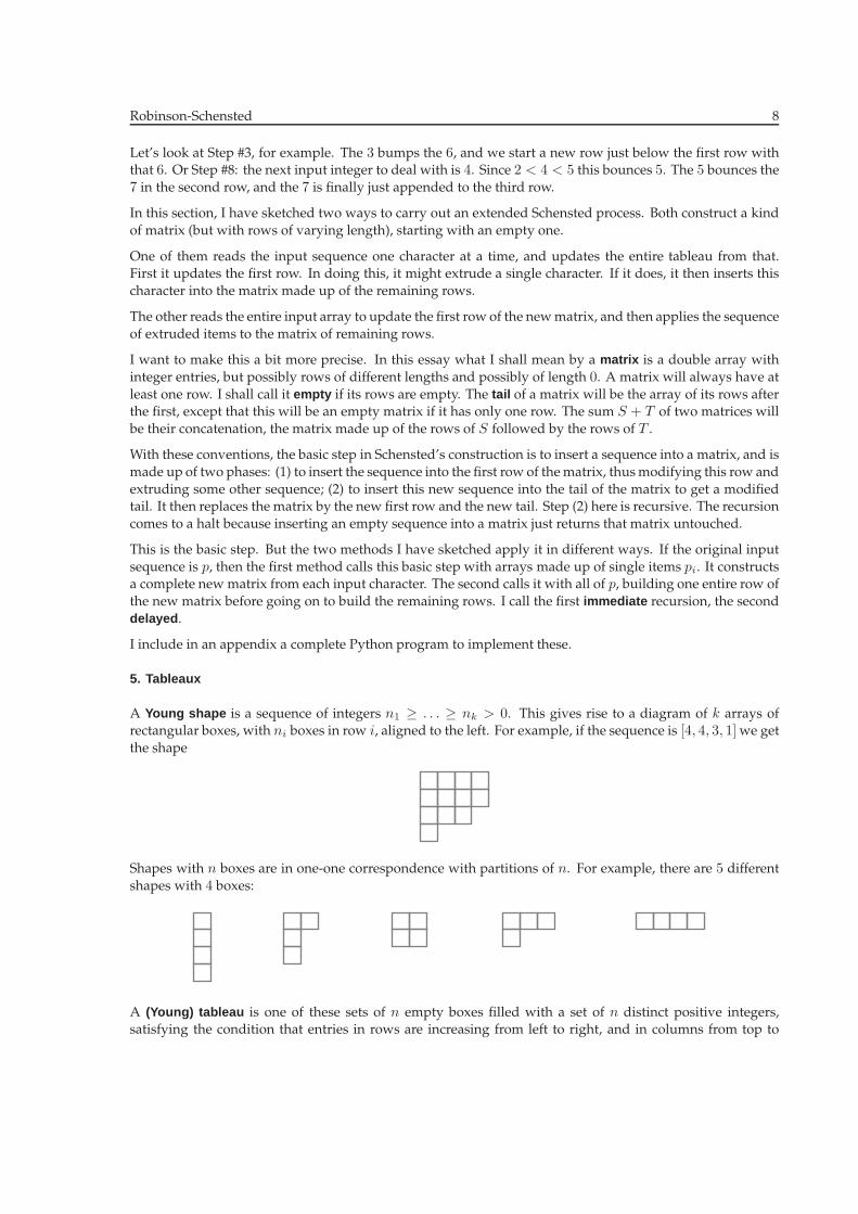
Let’s look at Step #3, for example. The 3 bumps the 6, and we start a new row just below the first row withthat 6. Or Step #8: the next input integer to deal with is 4. Since 2 < 4 < 5 this bounces 5. The 5 bounces the
7 in the second row, and the 7 is finally just appended to the third row.
In this section, I have sketched two ways to carry out an extended Schensted process. Both construct a kind
of matrix (but with rows of varying length), starting with an empty one.
One of them reads the input sequence one character at a time, and updates the entire tableau from that.First it updates the first row. In doing this, it might extrude a single character. If it does, it then inserts this
character into the matrix made up of the remaining rows.
The other reads the entire input array to update the first row of the newmatrix, and then applies the sequence
of extruded items to the matrix of remaining rows.
I want to make this a bit more precise. In this essay what I shall mean by a matrix is a double array with
integer entries, but possibly rows of different lengths and possibly of length 0. A matrix will always have at
least one row. I shall call it empty if its rows are empty. The tail of a matrix will be the array of its rows afterthe first, except that this will be an empty matrix if it has only one row. The sum S + T of two matrices will
be their concatenation, the matrix made up of the rows of S followed by the rows of T .
With these conventions, the basic step in Schensted’s construction is to insert a sequence into a matrix, and is
made up of two phases: (1) to insert the sequence into the first row of thematrix, thusmodifying this row and
extruding some other sequence; (2) to insert this new sequence into the tail of the matrix to get a modifiedtail. It then replaces the matrix by the new first row and the new tail. Step (2) here is recursive. The recursion
comes to a halt because inserting an empty sequence into a matrix just returns that matrix untouched.
This is the basic step. But the two methods I have sketched apply it in different ways. If the original input
sequence is p, then the first method calls this basic step with arrays made up of single items pi. It constructsa complete newmatrix from each input character. The second calls it with all of p, building one entire row of
the new matrix before going on to build the remaining rows. I call the first immediate recursion, the second
delayed .
I include in an appendix a complete Python program to implement these.
5. Tableaux
A Young shape is a sequence of integers n1 ≥ . . . ≥ nk > 0. This gives rise to a diagram of k arrays ofrectangular boxes, with ni boxes in row i, aligned to the left. For example, if the sequence is [4, 4, 3, 1]we get
the shape
Shapes with n boxes are in oneone correspondence with partitions of n. For example, there are 5 different
shapes with 4 boxes:
A (Young) tableau is one of these sets of n empty boxes filled with a set of n distinct positive integers,satisfying the condition that entries in rows are increasing from left to right, and in columns from top to
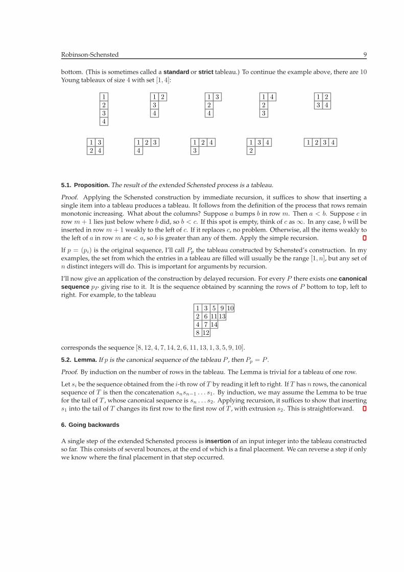
RobinsonSchensted 9
bottom. (This is sometimes called a standard or strict tableau.) To continue the example above, there are 10Young tableaux of size 4 with set [1, 4]:
1234
1 234
1 324
1 423
1 23 4
1 32 4
1 2 34
1 2 43
1 3 42
1 2 3 4
5.1. Proposition. The result of the extended Schensted process is a tableau.
Proof. Applying the Schensted construction by immediate recursion, it suffices to show that inserting asingle item into a tableau produces a tableau. It follows from the definition of the process that rows remain
monotonic increasing. What about the columns? Suppose a bumps b in row m. Then a < b. Suppose c in
row m + 1 lies just below where b did, so b < c. If this spot is empty, think of c as∞. In any case, b will beinserted in row m + 1 weakly to the left of c. If it replaces c, no problem. Otherwise, all the items weakly to
the left of a in row m are < a, so b is greater than any of them. Apply the simple recursion.
If p = (pi) is the original sequence, I’ll call Pp the tableau constructed by Schensted’s construction. In my
examples, the set from which the entries in a tableau are filled will usually be the range [1, n], but any set of
n distinct integers will do. This is important for arguments by recursion.
I’ll now give an application of the construction by delayed recursion. For every P there exists one canonicalsequence pP giving rise to it. It is the sequence obtained by scanning the rows of P bottom to top, left toright. For example, to the tableau
1 3 5 9 102 6 11 134 7 148 12
corresponds the sequence [8, 12, 4, 7, 14, 2, 6, 11, 13, 1, 3, 5, 9, 10].
5.2. Lemma. If p is the canonical sequence of the tableau P , then Pp = P .
Proof. By induction on the number of rows in the tableau. The Lemma is trivial for a tableau of one row.
Let si be the sequence obtained from the ith row of T by reading it left to right. If T has n rows, the canonical
sequence of T is then the concatenation snsn−1 . . . s1. By induction, we may assume the Lemma to be truefor the tail of T , whose canonical sequence is sn . . . s2. Applying recursion, it suffices to show that inserting
s1 into the tail of T changes its first row to the first row of T , with extrusion s2. This is straightforward.
6. Going backwards
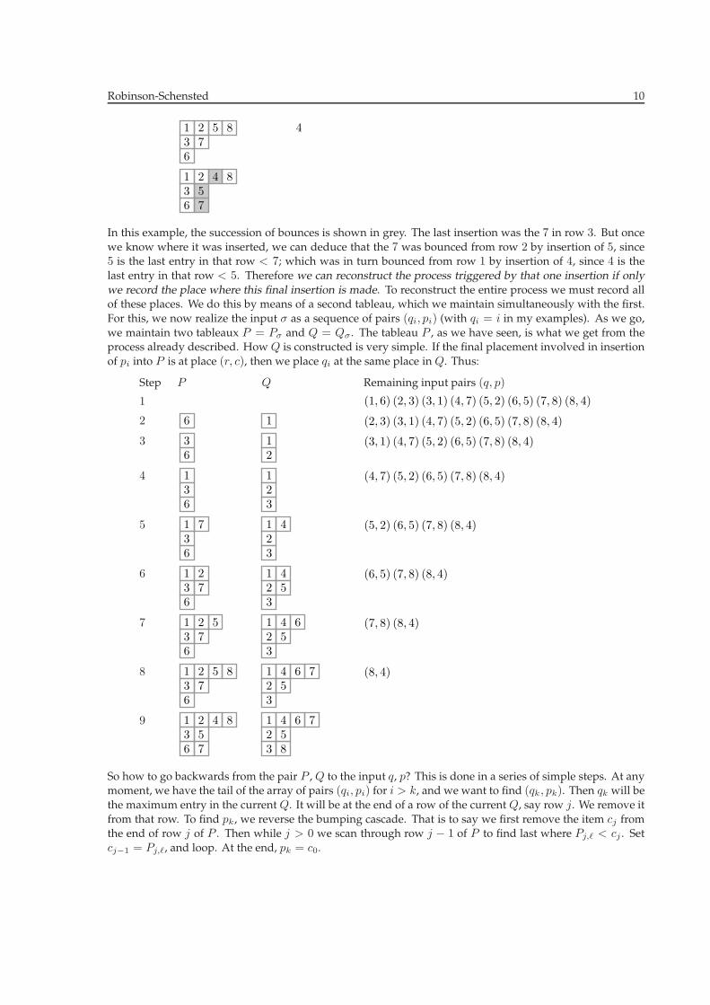
A single step of the extended Schensted process is insertion of an input integer into the tableau constructedso far. This consists of several bounces, at the end of which is a final placement. We can reverse a step if only
we know where the final placement in that step occurred.
RobinsonSchensted 10
41 2 5 83 76
1 2 4 83 56 7
In this example, the succession of bounces is shown in grey. The last insertion was the 7 in row 3. But oncewe know where it was inserted, we can deduce that the 7 was bounced from row 2 by insertion of 5, since5 is the last entry in that row < 7; which was in turn bounced from row 1 by insertion of 4, since 4 is the
last entry in that row < 5. Therefore we can reconstruct the process triggered by that one insertion if onlywe record the place where this final insertion is made. To reconstruct the entire process we must record allof these places. We do this by means of a second tableau, which we maintain simultaneously with the first.
For this, we now realize the input σ as a sequence of pairs (qi, pi) (with qi = i in my examples). As we go,
we maintain two tableaux P = Pσ and Q = Qσ. The tableau P , as we have seen, is what we get from theprocess already described. How Q is constructed is very simple. If the final placement involved in insertion
of pi into P is at place (r, c), then we place qi at the same place in Q. Thus:
Step P Q Remaining input pairs (q, p)
1 (1, 6) (2, 3) (3, 1) (4, 7) (5, 2) (6, 5) (7, 8) (8, 4)
2 (2, 3) (3, 1) (4, 7) (5, 2) (6, 5) (7, 8) (8, 4)16
3 (3, 1) (4, 7) (5, 2) (6, 5) (7, 8) (8, 4)1326
4 (4, 7) (5, 2) (6, 5) (7, 8) (8, 4)112336
5 (5, 2) (6, 5) (7, 8) (8, 4)11 472336
6 (6, 5) (7, 8) (8, 4)11 4223 5736
7 (7, 8) (8, 4)11 42 6523 5736
8 (8, 4)11 42 65 7823 5736
9 11 42 64 7823 5536 87
So how to go backwards from the pair P , Q to the input q, p? This is done in a series of simple steps. At anymoment, we have the tail of the array of pairs (qi, pi) for i > k, and we want to find (qk, pk). Then qk will be
the maximum entry in the current Q. It will be at the end of a row of the current Q, say row j. We remove it
from that row. To find pk, we reverse the bumping cascade. That is to say we first remove the item cj fromthe end of row j of P . Then while j > 0 we scan through row j − 1 of P to find last where Pj,ℓ < cj . Set
cj−1 = Pj,ℓ, and loop. At the end, pk = c0.
RobinsonSchensted 11
For the moment, call p = (pi) an admissible sequence if (1) the pi are positive integers and (2) all the pi aredistinct. Define {p} to be the set of all the pi. Similarly, if P is a tableau, let {P} be the set of its entries.
6.1. Theorem. The map taking (p, q) to (P, Q) is a bijection between pairs p, q of admissible sequences of thesame length and pairs of tableaux P , Q of the same shape with {P} = {p}, {Q} = {q}.
If we apply this to permutations σ, giving rise to sequences (i, σi), this leads to:
6.2. Corollary. Themap σ 7→ (Pσ, Qσ) is a bijection of the group of permutationswith pairs of Young tableauxof the same shape and entries in [1, n].
Here is what we get for S3:
σ word expression P Q
1 2 3 I 1 2 3 1 2 3
2 1 3 s1 12
3 12
3
2 3 1 s1s2 12
3 13
2
1 3 2 s2 13
2 13
2
3 1 2 s2s1 13
2 12
3
3 2 1 s1s2s1 = s2s1s2
321
321
The Robinson-Schensted correspondence is the bijection defined in this section between permutations and
pairs (P, Q)of tableaux of the same shape. With the advent of cells andW graphs (in [KazhdanLusztig:1979])it has acquired a new significance.
7. Delayed pair processing
In the process described in the previous section, we are given a sequence of pairs (qi, pi). In each step, a singleinteger pi is inserted into a tableau, and qi is inserted into a second tableau. Thus tableaux are modified (or
enlarged) upon reading each new input pair. But here also one can speak of delayed insertion. It constructs
only a pair of corresponding rows ofP andQ by postponing insertion in lower rows until one has completelyconstructed the first row.
First of all, I now allow as input any sequence of pairs (pi, qi) with qi not necessarily equal to i, but at leastordered so that qi < qj if i < j. We can apply the previous process to such a sequence, placing qi where
before we placed i. This generalization will now prove significant.
Instead of inserting a pair (qi, pi) and getting two new tableaux, the basic step now will be just to insert pi
into a row P . What happens to qi depends on how pi is inserted. (a) If pi is appended to the row, we append
qi to a second row Q. Otherwise (b) pi will bounce some rℓ. In this case, add the pair (rℓ, qi) at the end of anew input sequence.
Here is how one example goes:
1 (1, 6) (2, 3) (3, 1) (4, 7) (5, 2) (6, 5) (7, 8) (8, 4)
2 (2, 3) (3, 1) (4, 7) (5, 2) (6, 5) (7, 8) (8, 4)6 1
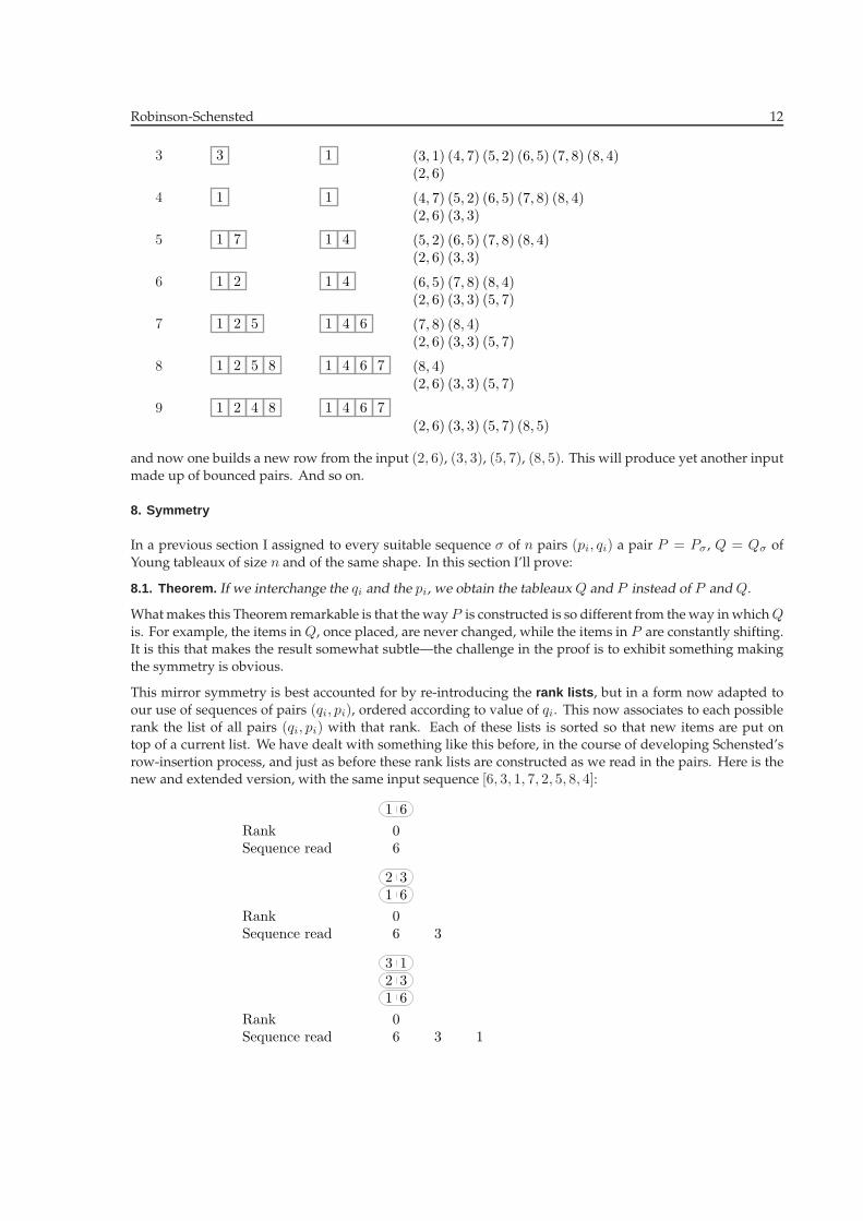
RobinsonSchensted 12
3 (3, 1) (4, 7) (5, 2) (6, 5) (7, 8) (8, 4)(2, 6)
3 1
4 (4, 7) (5, 2) (6, 5) (7, 8) (8, 4)(2, 6) (3, 3)
1 1
5 (5, 2) (6, 5) (7, 8) (8, 4)(2, 6) (3, 3)
1 17 4
6 (6, 5) (7, 8) (8, 4)(2, 6) (3, 3) (5, 7)
1 12 4
7 (7, 8) (8, 4)(2, 6) (3, 3) (5, 7)
1 12 45 6
8 (8, 4)(2, 6) (3, 3) (5, 7)
1 12 45 68 7
9(2, 6) (3, 3) (5, 7) (8, 5)
1 12 44 68 7
and now one builds a new row from the input (2, 6), (3, 3), (5, 7), (8, 5). This will produce yet another input
made up of bounced pairs. And so on.
8. Symmetry
In a previous section I assigned to every suitable sequence σ of n pairs (pi, qi) a pair P = Pσ , Q = Qσ of
Young tableaux of size n and of the same shape. In this section I’ll prove:
8.1. Theorem. If we interchange the qi and the pi, we obtain the tableaux Q and P instead of P and Q.
Whatmakes this Theorem remarkable is that theway P is constructed is so different from theway inwhichQis. For example, the items in Q, once placed, are never changed, while the items in P are constantly shifting.It is this that makes the result somewhat subtle—the challenge in the proof is to exhibit something making
the symmetry is obvious.
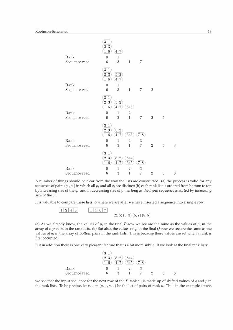
This mirror symmetry is best accounted for by reintroducing the rank lists , but in a form now adapted to
our use of sequences of pairs (qi, pi), ordered according to value of qi. This now associates to each possible
rank the list of all pairs (qi, pi) with that rank. Each of these lists is sorted so that new items are put ontop of a current list. We have dealt with something like this before, in the course of developing Schensted’s
rowinsertion process, and just as before these rank lists are constructed as we read in the pairs. Here is thenew and extended version, with the same input sequence [6, 3, 1, 7, 2, 5, 8, 4]:
Sequence readRank 0
6
1 6
Sequence readRank 0
6 3
1 62 3
Sequence readRank 0
6 3 1
1 62 33 1
RobinsonSchensted 13
Sequence readRank 0 1
6 3 1 7
1 62 33 1
4 7
Sequence readRank 0 1
6 3 1 7 2
1 62 33 1
4 75 2
Sequence readRank 0 1 2
6 3 1 7 2 5
1 62 33 1
4 75 2
6 5
Sequence readRank 0 1 2 3
6 3 1 7 2 5 8
1 62 33 1
4 75 2
6 5 7 8
Sequence readRank 0 1 2 3
6 3 1 7 2 5 8
1 62 33 1
4 75 2
6 5 7 88 4
A number of things should be clear from the way the lists are constructed: (a) the process is valid for any
sequence of pairs (qi, pi) in which all pi and all qi are distinct; (b) each rank list is ordered from bottom to top
by increasing size of the qi, and in decreasing size of pi, as long as the input sequence is sorted by increasingsize of the qi.
It is valuable to compare these lists to where we are after we have inserted a sequence into a single row:
(2, 6) (3, 3) (5, 7) (8, 5)
1 12 44 68 7
(a) As we already know, the values of pi in the final P row we see are the same as the values of pi in thearray of top pairs in the rank lists. (b) But also, the values of qi in the final Qrow we see are the same as the
values of qi in the array of bottom pairs in the rank lists. This is because these values are set when a rank is
first occupied.
But in addition there is one very pleasant feature that is a bit more subtle. If we look at the final rank lists:
Sequence readRank 0 1 2 3
6 3 1 7 2 5 8
1 62 33 1
4 75 2
6 5 7 88 4
we see that the input sequence for the next row of the P tableau is made up of shifted values of q and p in
the rank lists. To be precise, let rn,i = (qn,i, pn,i) be the list of pairs of rank n. Thus in the example above,
RobinsonSchensted 14
r0,0 = (1, 6), r0,1 = (2, 3). To get the next input, we scan through all the rank lists starting at rank 0, takingthe p values from the pairs rn,i and the qvalues from rn,i+1. Thus in the example above we have
(2, 6)(3, 3)(5, 7)(8, 5) = (q0,1, p0,0)(q0,2, p0,1)(q1,1, p1,0)(q2,1, p2,0) .
This is always true: the next input sequence is made up of pairs p from the rn,i and q from rn,i+1 (sortedaccording to size of the values of q). In other words, the rank lists encode very neatly the results of insertioninto a single row.
Now the content of the rank lists is a canonical invariant of the original set of pairs (qi, pi), independent ofany ordering assigned to them. This is because the rank is that in a partially ordered set defined by the pairs.
If we swap the sequences q and p, we get the same rank lists, but each one reversed in order. An induction
argument then proves that if we swap q and p we swap P and Q.
In terms of permutations in Sn:
8.2. Corollary. If σ in Sn maps to (P, Q) with respect to the RobinsonSchensted correspondence, its inverseσ−1 maps to (Q, P ).
9. Appendix. Python code
The initialization gives T enough rows to hold all of the input. Only rarely will all be needed, and at the endblank rows are removed. Throughout, p is an array of zero or more nonnegative integers.
The subroutines here all modify the initial tableau. This behaviour is slightly different from normal mathematical usage. For example, a matrix in mathematics is a strictly rectangular array. It is common enough
in normal usage to modify its entries—for example, in Gauss elimination—but not its dimensions. Whereasin most programming languages, a matrix is usually an array of arrays, which may be of any length, not
necessarily all of the same length, and even extended in the course of a program.
I havewritten this program to use recursion, because it is easy to justify in standardmathematical terms. Morecommonly in programs, however, one would us while loops and justify the program by putting ‘assertions’
into the loop, explaining the state of affairs at each entrance and proving that such an assertion remains validain the course of the loop. But this is not easy to explain in mathematical terms. (But then in mathematical
terms, how do you explain easily a statement like n = n+1?)
Few of the features used here are unique to Python. You might want to keep in mind, however, that if r is an
array then r[-1] is its final entry.
# --- inserting items one by one ----------------------------
def P_simple(p):
n = len(p)
T = empty_matrix(n)
for m in p:
insert_into_tableau(T, [m])
while len(T) > 0 and len(T[-1]) == 0:
T.pop()
return T
# --- delayed insertion ---------------------------------------
# returns the new tableau
def P(p):
n = len(p)
T = empty_matrix(n)
RobinsonSchensted 15
insert_into_tableau(T, p)
while len(T) > 0 and len(T[-1]) == 0:
T.pop()
return T
# --- common to both ------------------------------------------
def insert_into_tableau(T, p):
if len(p) == 0:
return T
q = insert_array_into_row(T[0], p) # q = array of bumped items
if len(q) > 0:
insert_into_tableau(T[1:], q)
return T # with modified R
# p is the input array of non-negative integers
# r is an increasing row of non-negative integers, possibly empty
# this modifies r, and returns the sequence q of items bumped
def insert_array_into_row(r, p):
a = []
for m in p:
b = insert_item_into_row(r, m)
a += b
return a
# returns [] if m tacked on, and [bumped item] otherwise
def insert_item_into_row(r, m):
N = len(r)
n = N
while n > 0 and m < r[n-1]:
n -= 1
# at end n = N or 0 <= n < N and r[n-1] < m < r[n]
# convention: r[-1] = -1, r[N] = infinity
if n == N:
r.append(m)
return []
else:
a = r[n]
r[n] = m
return [a]
def empty_matrix(n):
T = []
for i in range(n+1):
T.append([])
return T
This program may also be found at
http://www.math.ubc.ca/~cass/python/robinson-schensted.py
Part II. Cells
RobinsonSchensted 16
10. Descents and tableaux
The RobinsonSchensted correspondence is a bijection between permutations in Sn and pairs of Young
tableaux of the same shape and size n. What properties of a permutation can be read off easily from thecorresponding tableaux?
I begin by asking the simple question, how does the final position of an item in the input sequence relate toits initial placement?
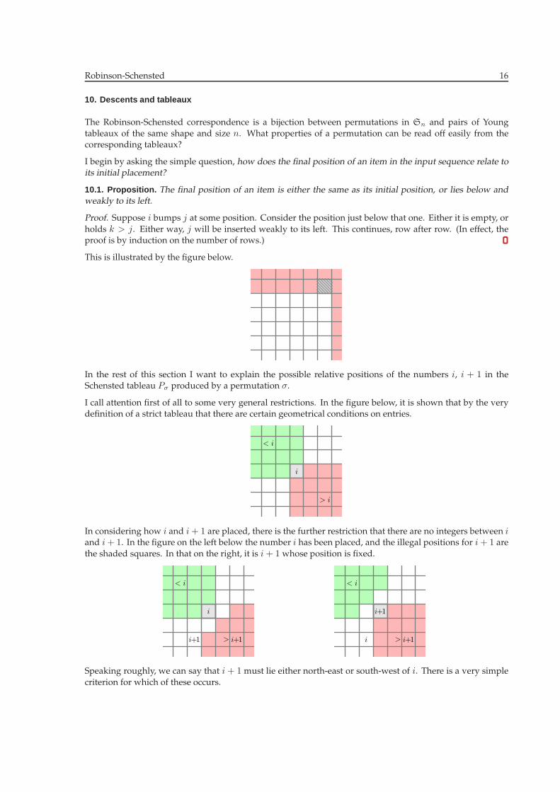
10.1. Proposition. The final position of an item is either the same as its initial position, or lies below andweakly to its left.
Proof. Suppose i bumps j at some position. Consider the position just below that one. Either it is empty, or
holds k > j. Either way, j will be inserted weakly to its left. This continues, row after row. (In effect, theproof is by induction on the number of rows.)
This is illustrated by the figure below.
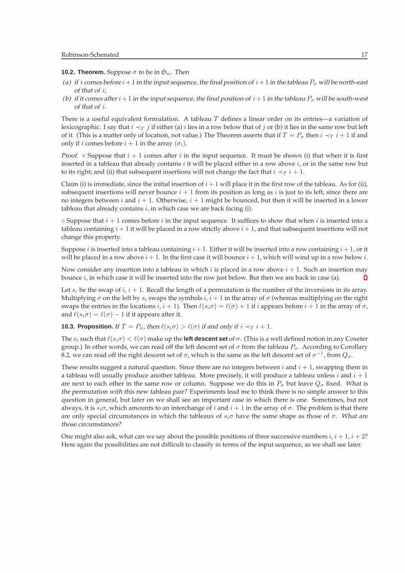
In the rest of this section I want to explain the possible relative positions of the numbers i, i + 1 in theSchensted tableau Pσ produced by a permutation σ.
I call attention first of all to some very general restrictions. In the figure below, it is shown that by the verydefinition of a strict tableau that there are certain geometrical conditions on entries.
i
> i
< i
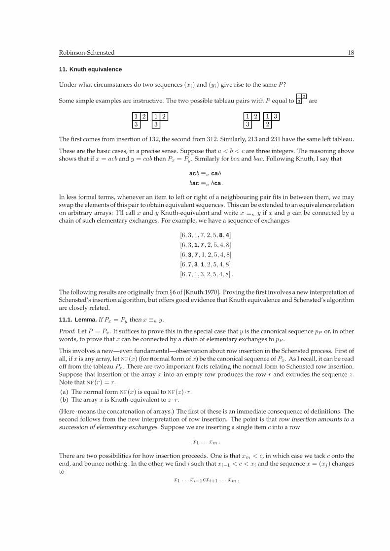
In considering how i and i + 1 are placed, there is the further restriction that there are no integers between iand i + 1. In the figure on the left below the number i has been placed, and the illegal positions for i + 1 are
the shaded squares. In that on the right, it is i + 1 whose position is fixed.
i
< i
> i+1i+1
i+1
< i
> i+1i
Speaking roughly, we can say that i + 1 must lie either northeast or southwest of i. There is a very simple
criterion for which of these occurs.
RobinsonSchensted 17
10.2. Theorem. Suppose σ to be in Sn. Then
(a) if i comes before i+1 in the input sequence, the final position of i+1 in the tableau Pσ will be northeastof that of i;
(b) if it comes after i+1 in the input sequence, the final position of i+1 in the tableau Pσ will be southwestof that of i.
There is a useful equivalent formulation. A tableau T defines a linear order on its entries—a variation oflexicographic. I say that i ≺T j if either (a) i lies in a row below that of j or (b) it lies in the same row but left
of it. (This is a matter only of location, not value.) The Theorem asserts that if T = Pσ then i ≺T i + 1 if and
only if i comes before i + 1 in the array (σi).
Proof. ◦ Suppose that i + 1 comes after i in the input sequence. It must be shown (i) that when it is first
inserted in a tableau that already contains i it will be placed either in a row above i, or in the same row butto its right; and (ii) that subsequent insertions will not change the fact that i ≺T i + 1.
Claim (i) is immediate, since the initial insertion of i+1 will place it in the first row of the tableau. As for (ii),subsequent insertions will never bounce i + 1 from its position as long as i is just to its left, since there are
no integers between i and i + 1. Otherwise, i + 1 might be bounced, but then it will be inserted in a lower
tableau that already contains i, in which case we are back facing (i).
◦ Suppose that i + 1 comes before i in the input sequence. It suffices to show that when i is inserted into a
tableau containing i + 1 it will be placed in a row strictly above i + 1, and that subsequent insertions will notchange this property.
Suppose i is inserted into a tableau containing i+1. Either it will be inserted into a row containing i+1, or itwill be placed in a row above i + 1. In the first case it will bounce i + 1, which will wind up in a row below i.
Now consider any insertion into a tableau in which i is placed in a row above i + 1. Such an insertion maybounce i, in which case it will be inserted into the row just below. But then we are back in case (a).
Let si be the swap of i, i + 1. Recall the length of a permutation is the number of the inversions in its array.Multiplying σ on the left by si swaps the symbols i, i + 1 in the array of σ (whereas multiplying on the right
swaps the entries in the locations i, i + 1). Then ℓ(siσ) = ℓ(σ) + 1 if i appears before i + 1 in the array of σ,and ℓ(siσ) = ℓ(σ)− 1 if it appears after it.
10.3. Proposition. If T = Pσ , then ℓ(siσ) > ℓ(σ) if and only if i ≺T i + 1.
The si such that ℓ(siσ) < ℓ(σ)make up the left descent set of σ. (This is a well defined notion in any Coxetergroup.) In other words, we can read off the left descent set of σ from the tableau Pσ . According to Corollary
8.2, we can read off the right descent set of σ, which is the same as the left descent set of σ−1, from Qσ.
These results suggest a natural question. Since there are no integers between i and i + 1, swapping them in
a tableau will usually produce another tableau. More precisely, it will produce a tableau unless i and i + 1are next to each other in the same row or column. Suppose we do this in Pσ but leave Qσ fixed. What isthe permutation with this new tableau pair? Experiments lead me to think there is no simple answer to this
question in general, but later on we shall see an important case in which there is one. Sometimes, but notalways, it is siσ, which amounts to an interchange of i and i + 1 in the array of σ. The problem is that there
are only special circumstances in which the tableaux of siσ have the same shape as those of σ. What arethose circumstances?
One might also ask, what can we say about the possible positions of three successive numbers i, i + 1, i + 2?Here again the possibilities are not difficult to classify in terms of the input sequence, as we shall see later.
RobinsonSchensted 18
11. Knuth equivalence
Under what circumstances do two sequences (xi) and (yi) give rise to the same P ?
Some simple examples are instructive. The two possible tableau pairs with P equal to 321are
321
321
321
231
The first comes from insertion of 132, the second from 312. Similarly, 213 and 231 have the same left tableau.
These are the basic cases, in a precise sense. Suppose that a < b < c are three integers. The reasoning aboveshows that if x = acb and y = cab then Px = Py . Similarly for bca and bac. Following Knuth, I say that
acb ≡κ cab
bac ≡κ bca .
In less formal terms, whenever an item to left or right of a neighbouring pair fits in between them, we may
swap the elements of this pair to obtain equivalent sequences. This can be extended to an equivalence relation
on arbitrary arrays: I’ll call x and y Knuthequivalent and write x ≡κ y if x and y can be connected by achain of such elementary exchanges. For example, we have a sequence of exchanges
[6, 3, 1, 7, 2, 5, 8, 4]
[6, 3, 1, 7 , 2, 5, 4, 8]
[6, 3, 7 , 1, 2, 5, 4, 8]
[6, 7, 3, 1, 2, 5, 4, 8]
[6, 7, 1, 3, 2, 5, 4, 8] .
The following results are originally from §6 of [Knuth:1970]. Proving the first involves a new interpretation ofSchensted’s insertion algorithm, but offers good evidence that Knuth equivalence and Schensted’s algorithm
are closely related.
11.1. Lemma. If Px = Py then x ≡κ y.
Proof. Let P = Px. It suffices to prove this in the special case that y is the canonical sequence pP or, in other
words, to prove that x can be connected by a chain of elementary exchanges to pP .
This involves a new—even fundamental—observation about row insertion in the Schensted process. First of
all, if x is any array, let NF(x) (for normal form of x) be the canonical sequence ofPx. As I recall, it can be readoff from the tableau Px. There are two important facts relating the normal form to Schensted row insertion.
Suppose that insertion of the array x into an empty row produces the row r and extrudes the sequence z.Note that NF(r) = r.
(a) The normal form NF(x) is equal to NF(z) ·r.(b) The array x is Knuthequivalent to z ·r.
(Here ·means the concatenation of arrays.) The first of these is an immediate consequence of definitions. The
second follows from the new interpretation of row insertion. The point is that row insertion amounts to asuccession of elementary exchanges. Suppose we are inserting a single item c into a row
x1 . . . xm .
There are two possibilities for how insertion proceeds. One is that xm < c, in which case we tack c onto the
end, and bounce nothing. In the other, we find i such that xi−1 < c < xi and the sequence x = (xj) changesto
x1 . . . xi−1cxi+1 . . . xm ,
RobinsonSchensted 19
and we bounce xi. In this second case, I claim that the array
xi ·x1 . . . c . . . xm
is Knuthequivalent to x ·c.
To verify this, first of all set j = m, and as long as c < xj−1 < xj we can change xj−1xjc to xj−1cxj , anddecrement j. (Here and elsewhere I adopt the harmless convention that x−1 = 0.)
At the end of this phase we are looking atxi−1xic
with xi−1 < c < xi. We leave c fixed in place (it has in effect just bounced xi) and now proceed similarly to
shift xi all the way to the left. This proves the claim, and by induction on the length of z proves (b) above.
But if we combine (a) and (b) with an induction hypothesis on the length of x for the Proposition, we get
x ≡κ z ·r ≡κ NF(z) ·r = NF(x) .
For example, if we insert 4 into (1, 2, 5, 8, 9) the 4 will bounce the 5. We get
1 2 5 8 9 4 ≡κ 1 2 5 8 4 9
= 1 2 5 8 4 9
≡κ 1 2 5 4 8 9
= 1 2 5 4 8 9
≡κ 1 5 2 4 8 9
= 1 5 2 4 8 9
≡κ 5 1 2 4 8 9 .
Now the converse.
11.2. Lemma. If x is a sequence (pi). and y ≡κ x, then Py = Px.
From this and the previous result:
11.3. Theorem. We have x ≡κ y if and only if Px = Py .
Proof of Lemma 11.2. The proof I’ll give here is straightforward if unilluminating. In the next section I’ll give
an alternate proof that I like better, but there is some virtue in the direct route outlined here, which amountsto the one hinted at in the answer to exercise 5.1.4.5 of [Knuth:1975]. A rather different proof of the Lemma
can be found in Chapter 3 of [Fulton:1997].
It must be shown that if x and y are related by an elementary interchange then Px = Py . Applying aninduction argument, it suffices to show that inserting x and y into a single row produce (a) the same new
row as well as (b) extrusions that are Knuthequivalent. It even suffices to assume that x and y are one of theKnuth triples acb etc.. The proof goes according to cases. There are several of these, and laying them all out
is somewhat tedious, if automatic.
I shall track the insertions of the triples acb, cab, bac, bca into the row x1 . . . xn. I shall allow n = 0 by
following the harmless convention that x0 = 0. I shall also use a trick suggested somewhere by Knuth—I
introduce several very, very large integers and assume an arbitrary number of them at the end of every row.If I then perform the Schensted process, all of these will get placed again at the ends of rows. They can then
finally be removed, leaving exactly the same tableau we would have had without using them. The point of
this is to shrink the number of cases, since now every insertion will bump something.
RobinsonSchensted 20
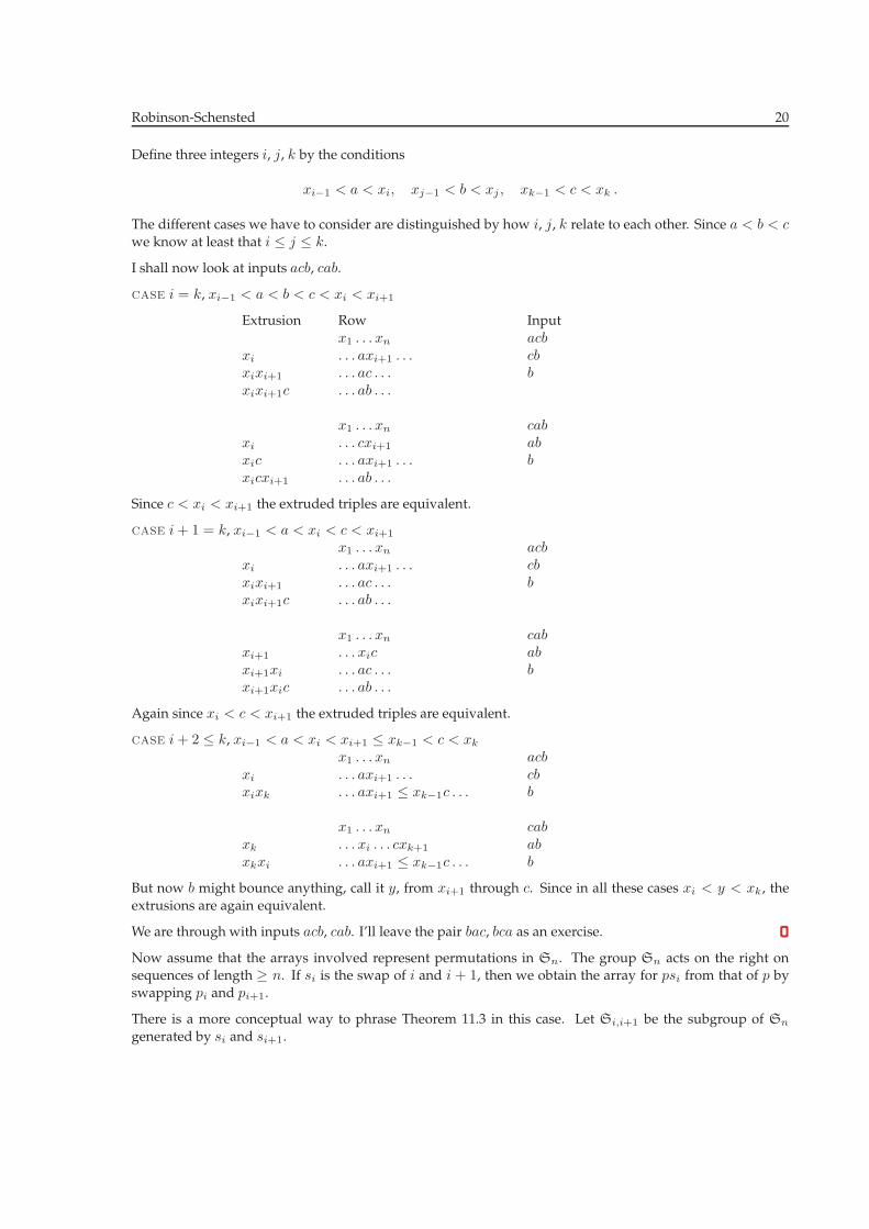
Define three integers i, j, k by the conditions
xi−1 < a < xi, xj−1 < b < xj , xk−1 < c < xk .
The different cases we have to consider are distinguished by how i, j, k relate to each other. Since a < b < cwe know at least that i ≤ j ≤ k.
I shall now look at inputs acb, cab.
CASE i = k, xi−1 < a < b < c < xi < xi+1
Extrusion Row Input
x1 . . . xn acbxi . . . axi+1 . . . cbxixi+1 . . . ac . . . bxixi+1c . . . ab . . .
x1 . . . xn cabxi . . . cxi+1 abxic . . . axi+1 . . . bxicxi+1 . . . ab . . .
Since c < xi < xi+1 the extruded triples are equivalent.
CASE i + 1 = k, xi−1 < a < xi < c < xi+1
x1 . . . xn acbxi . . . axi+1 . . . cbxixi+1 . . . ac . . . bxixi+1c . . . ab . . .
x1 . . . xn cabxi+1 . . . xic abxi+1xi . . . ac . . . bxi+1xic . . . ab . . .
Again since xi < c < xi+1 the extruded triples are equivalent.
CASE i + 2 ≤ k, xi−1 < a < xi < xi+1 ≤ xk−1 < c < xk
x1 . . . xn acbxi . . . axi+1 . . . cbxixk . . . axi+1 ≤ xk−1c . . . b
x1 . . . xn cabxk . . . xi . . . cxk+1 abxkxi . . . axi+1 ≤ xk−1c . . . b
But now b might bounce anything, call it y, from xi+1 through c. Since in all these cases xi < y < xk, the
extrusions are again equivalent.
We are through with inputs acb, cab. I’ll leave the pair bac, bca as an exercise.
Now assume that the arrays involved represent permutations in Sn. The group Sn acts on the right onsequences of length ≥ n. If si is the swap of i and i + 1, then we obtain the array for psi from that of p by
swapping pi and pi+1.
There is a more conceptual way to phrase Theorem 11.3 in this case. Let Si,i+1 be the subgroup of Sn
generated by si and si+1.
RobinsonSchensted 21
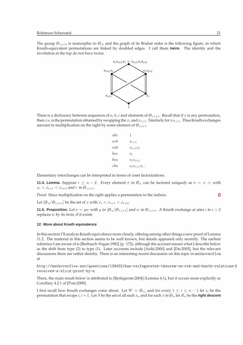
The group Si,i+1 is isomorphic to S3, and the graph of its Bruhat order is the following figure, in whichKnuthequivalent permutations are linked by doubled edges. I call them twins . The identity and the
involution at the top do not have twins.
sisi+1si = si+1sisi+1
1
sisi+1
sisi+1si+1si
There is a dictionary between sequences of a, b, c and elements of Si,i+1. Recall that if x is any permutation,
thenxsi is the permutation obtainedby swapping thexi andxi+1 . Similarly forxsi+1 . ThusKnuth exchangesamount to multiplication on the right by some element of Si,i+1.
abc 1
acb si+1
cab si+1si
bac si
bca sisi+1
cba sisi+1si .
Elementary interchanges can be interpreted in terms of coset factorizations.
11.4. Lemma. Suppose i ≤ n − 2. Every element σ in Sn can be factored uniquely as σ = x · τ , withxi < xi+1 < xi+2 and τ in Si,i+1.
Proof. Since multiplication on the right applies a permutation to the indices.
Let [Sn/Si,i+1] be the set of x with xi < xi+1 < xi+2.
11.5. Proposition. Let x = yw with y in [Sn/Si,i+1] and w in Si,i+1. A Knuth exchange at sites i to i + 2replaces w by its twin, if it exists.
12. More about Knuth equivalence
In this section I’ll analyze Knuth equivalencemore closely, offering among other things a newproof of Lemma11.2. The material in this section seems to be well known, but details appeared only recently. The earliest
reference I am aware of is [BarbaschVogan:1982] (p. 172), although the account misses what I describe below
as the shift from type (2) to type (1). Later accounts include [Ariki:2000] and [Du:2005], but the relevantdiscussions there are rather sketchy. There is an interesting recent discussion on this topic in mathoverflow
at
http://mathoverflow.net/questions/139432/has-reifegerstes-theorem-on-rsk-and-knuth-relations-
received-a-slick-proof-by-n
There, the main result below is attributed to [Reifegerste:2004] (Lemma 4.1), but it occurs more explicitly as
Corollary 4.2.1 of [Post:2009].
I first recall how Knuth exchanges come about. Let W = Sn, and for every 1 ≤ i ≤ n − 1 let si be thepermutation that swaps i, i+1. Let S be the set of all such si, and for each x inSn letRx be the right descent
RobinsonSchensted 22
set of x, made up of the s in S such that xs < x (which by definition means that ℓ(xs) < ℓ(x)). Similarly, letLx be its left descent set.
There is a right Knuth exchange x 7→ x|i,i+1 defined on a subset of W for every 1 ≤ i ≤ n− 2. Suppose i inthis range, and suppose x to be a permutation with xi < xi+1 < xi+2, Then the Knuth exchange swaps
xsi ←→ xsisi+1
xsi+1 ←→ xsi+1si .
It is not defined on all of W . Its domain of definition is the set DR(i, i + 1) of those x for which the set
Rx(i, i + 1) = {si, si+1} ∩Rx
is a singleton. It is an involution of DR(i, i + 1).
One can also define a left Knuth exchange x 7→ i,i+1|x with domain DL(i, i + 1), those x for which
Lx(i, i + 1) = {si, si+1} ∩ Lx
is a singleton.
Lemma 11.2 tells us that if y = x|i,i+1 then Px = Py (as I’ll reprove in a little while). Theorem 10.2 applied tox−1, together with Corollary 8.2, tells us that we can determine from Qx alone whether x is in DR(i, i + 1).I’ll summarize here what we know.
As I have mentioned earlier, each tableau T determines an order on its entries, in terms of their locations. I’ll
say that i ≺T j if either (1) i lies in a row below j or (2) i lies in the same row as j but to its left. Thus Theorem10.2 says that if T = Px then i comes before i + 1 in the array (xj) if and only if i ≺T i + 1. Translating thisto x−1:
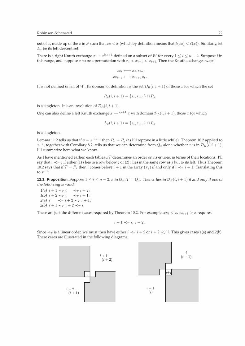
12.1. Proposition. Suppose 1 ≤ i ≤ n− 2, x in Sn, T = Qx. Then x lies in DR(i, i + 1) if and only if one ofthe following is valid:
1(a) i + 1 ≺T i ≺T i + 2;1(b) i + 2 ≺T i ≺T i + 1;2(a) i ≺T i + 2 ≺T i + 1;2(b) i + 1 ≺T i + 2 ≺T i.
These are just the different cases required by Theorem 10.2. For example, xsi < x, xsi+1 > x requires
i + 1 ≺T i, i + 2 .
Since ≺T is a linear order, we must then have either i ≺T i + 2 or i + 2 ≺T i. This gives cases 1(a) and 2(b).
These cases are illustrated in the following diagrams.
i
i+ 1(i+ 2)
i+ 2(i+ 1)
i+2
i(i + 1)
i + 1(i)
RobinsonSchensted 23
One has to be a bit careful in interpreting these. For example, if x = [2, 3, 1] then 3 occurs before 1 in x, but
T = Px is 231so that 1 ≺T 3.
The next natural question is, how is Qy related to Qx? Since a Knuth exchange doesn’t change Px, we expect
Qy to differ from Qx only in the positions of i, i + 1, or i + 2.
12.2. Theorem. Suppose 1 ≤ i ≤ n− 2, x in Sn, and suppose x is inDR(i, i + 1). In these circumstances, lety = x|i,i+1. Then Px = Py , and the tableau Qy is derived from Qx by swapping the two extreme items inthe relevant list of Proposition 12.1.
Thus 1(a) and 1(b) are swapped, as are 2(a) and 2(b).
Let’s look at an example. Suppose the input sequence is x = [1, 5, 7, 3, 10, 8, 4, 6, 2, 9]. At positions 8, 9, 10we have the bac segment [6, 2, 9], and the Knuth transform of x is y = [1, 5, 7, 3, 10, 8, 4, 6, 9, 2]. The tableauxQx and Qy are
1 2 3 5 104 6 879
1 2 3 5 94 6 8710
The diagonals emphasize the central items.
There is something slightly subtle about this result—the swap in Qx is not necessarily the same as the swap
in x. If x contains bac at positions i, i+1, i+2with a < b < c, and y replaces this by bca, then in all cases Qy
is obtained from Qx by swapping i + 1 and i + 2. But if x contains acb at the same positions and y replacesthis by cab, then it can happen that either i and i + 1 or i + 1 and i + 2 are swapped. For example, first let
x = [3, 1, 5, 2, 4] with a pattern acb at positions 2, 3, 4. The matrix Qx is shown at the left below.
1 3 52 4
1 3 524
Then let x = [4, 1, 3, 2, 5] with the same pattern at the same position. The matrix Qx is at the right.
What is going on reflects a fundamental difference between configurations of type (1), in which i is in themiddle, and those of type (2), in which i + 2 is in the middle. The first are stable, in the sense that successive
insertions will not change the type of the configuration. But the second can change (necessarily permanently)to a type (1) configuration. This happens when either i is inserted into a row in which i + 1, i + 2 occur, in
which case i + 1 is bounced, or i + 1 is inserted into a row in which i, i + 2 occur, in which case i + 2 is
bounced.
Proof of Theorem 12.2. The first step is to interpret the result as an assertion about the inverse of x. Corollary8.2 tells us that if y = x−1 then Py = Qx and Qy = Px. This allows us an easy translation. For example, ifthe Knuth triple acb occurs in positions i, i + 1, i + 2 of x then
x−1:
{
a 7→ ic 7→ i + 1b 7→ i + 2 .
In the Schensted process for X = x−1 the indices a, b, c are met in that order, so in X we first encounter i,then i + 2, and then i + 1. In the first example above
X = [1, 9, 4, 7, 2, 8, 3, 6, 10, 5] .
and sure enough 9, 8, 10 appear in that order.

RobinsonSchensted 24
So, replacing x by x−1, we now have two things to prove.
(1) Suppose x to contain in order i + 1, i, i + 2 while y differs from x only in swapping i + 2 and i + 1. We
wish to show that Qx = Qy and that Py is obtained from Px by swapping i + 1 and i + 2.
(2) Suppose x to contain in order i, i + 2, i + 1 while y differs from x only in swapping i and i + 1. The firstthing we wish to show is that Qx = Qy. As for Px and Py , I apply , applied to x0−1. Depending on whether
(1) or case (2) of of that Proposition occurs, we wish to show that either i + 1 and i + 2 or i and i + 1 areswapped.
The basic idea in both cases is the same. Let x≤m be the sequence of xi for i ≤ m, and similarly for y≤m.Also, let Px,n be the tableau corresponding to x≤n, and similarly Py,n, Qx,n, Qy,n. By convention, any of
these is an empty tableau for n = 0.
First, case (1). Suppose i+1, i, and i+2 to occur in x at positions k, ℓ, m, so y holds i+2, i, and i+1 at those
same positions. We read in x and y item by item. I claim that as we do this Qx,n is always equal to Qy,n, and
that Px,n differs from Py,n only in that where Px,n holds i + 1 (resp. i + 2) and Py,n holds i + 2 (resp. i + 1).
These claims are certainly true for n < k. What happens for n = k? For x we insert i + 1 into the top row
of Px,k−1 and for y we insert i + 2 into the top row of Py,k−1. But these top rows are the same, say r, andrj < i + 1 < rj+1 if and only if rj < i + 2 < rj+1 since r does not intersect [i, i + 2]. Therefore i + 1 is
inserted in the top row of Px,k−1 at the same location as i + 2 is inserted in that of Py,k−1, and the same item
is bounced into the common lower rows of both. Thus Px,k differs from Py,k only in that i + 2 is located inPy,k where i + 1 is located in Px,k and Qx,k = Qy,k. Since xn = yn for n in [k + 1, ℓ− 1], this remains true
up through n = ℓ− 1.
This illustrates the basic principle: inserting j into a tableau that does not contain j + 1 has the same effect
as inserting j + 1 into one that does not contain j.
What happens at n = ℓ? Well, i will bounce i + 1 from Px,ℓ−1 if and only if it bounces i + 2 from Py,ℓ−1, and
it will bounce it to the same location. So our claim remains valid for n = ℓ. In effect, i + 1 and i + 2 behave
exactly the same as input, and Theorem 10.2 may be applied to both. This guarantees that our claim remainsvalid for n < m.
What happens for n = m? Well, i is located NE of i + 1 in Px,m−1 and it is located NE of i + 2 in Py,m−1,so inserting i + 1 in Py,m−1 has exactly the same effect as inserting i + 2 into Px,m−1, and the claim remains
valid for n = m. The remaining input does not affect this.
Case (2) is essentially the same, except that in the final insertion of n = m something new can happen, if the
first row of Px,m−1 contains i, i + 2. In this case, i + 1 bumps i + 2, which is then inserted in a lower tableau,
leaving i, i + 1 in the first row. What happens for y? Since the claim is valid for n = m− 1, the first row of ycontains i + 1, i + 2, and i bumps i + 1, leaving i, i + 2 in the first row. We are now back in case (1).
There is an important consequence—one can tell just from the tableau Qx what right Knuth transforms arepossible, and how to determine Qy if y is such a transform. Equivalently, one can tell from Px what left
Knuth transforms are possible, and how to effect them.
If c is a chain of pairs (si, si+1), we can define the domainDL(c) as well as the operator x 7→ c|x from DL(c)to W by induction—if c is the juxtaposition of (i, i + 1) and d then DL(c) is the subset of DL(i, i + 1) suchthat i,i+1|x lies in DL(d), and then c|x = i,i+1|d|x.
Define≡r to mean right Knuthequivalence.
12.3. Corollary. If x and y are two permutations such that x ≡r y, then x is in DL(c) if and only if y is, andthen c|x ≡r
c|y.
This is crucial in proving that for Sn the Knuth equivalence classes coincide with the cells defined by
[KazhdanLusztig:1979].

RobinsonSchensted 25
Part III. References
1. Susumu Ariki, ‘RobinsonSchensted algorithm and left cells’, Advanced Studies in Pure Mathematics28 (2000), 1–20.
2. Dan Barbasch and David Vogan, ‘Primitive ideals and orbital integrals’, Mathematische Annalen 259(1982), 153–199.
3. Jie Du, ‘RobinsonSchensted algorithm and Vogan equivalence’, Journal of Combinatorial Theory 112(2005), 165–172.
4. William Fulton, Young diagrams , Cambridge University Press, 1997.
5. A. M. Garsia and T. J. McLarnan, ‘Relations between Young’s natural and the KazhdanLusztig repre
sentations of Sn’, Advances in Mathematics 69 (1988), 32–92.
6. David Kazhdan and George Lusztig, ‘Representations of Coxeter groups and Hecke algebras’, Inventiones Mathematicae 53 (1979), 165–184.
7. Donald Ervin Knuth, ‘Permutations, matrices, and generalized Young tableaux’, Pacific Journal ofMathematics 34 (1970), 709–727. Also to be found in the collection Selected papers on discrete mathematics ,CSLI, Stanford, 2003.
8. ——, Fundamental algorithms , volume I of The Art of Computer Programming , AddisonWesley, 1973.
9. ——, Sorting and Searching , volume III of The Art of Computer Programming , AddisonWesley, 1975.
10. Jacob Post, ‘Combinatorics of arc diagrams, Ferrers fillings, Young tableaux and lattice paths’, Ph. D.Thesis, Simon Fraser University, 2009.
11. Astrid Reifegerste, ‘Permutation sign under the RobinsonSchensted correspondence’, Annals of Combinatorics 8 (2004), 103–112.
12. C. Schensted, ‘Longest increasing and decreasing subsequences’, Canadian Journal of Mathematics 12(1963), 117–128.
13. Robert Steinberg, ‘An occurrence of the RobinsonSchensted correspondence’, Journal of Algebra 113(1988), 523–528.


![A Robinson-Schensted-Type Correspondence for a Dual Pair on … · 2017. 2. 6. · Recently, Date et al. [DaJiM] showed, using the representation of the quantized enveloping algebra](https://img.pdfslide.net/doc/110x75/60ab91f256f75a6489517d48/a-robinson-schensted-type-correspondence-for-a-dual-pair-on-2017-2-6-recently.jpg)