Rank Incentives

Evidence from a Randomized Workplace Experiment∗

Iwan Barankay†

July 7, 2012§

Abstract

Performance rankings are a very common workplace management practice. Behavioral theories suggest that providing performance rankings to employees, even without pecuniary consequences, may directly shape effort due to the rank’s effect on self-image. In a three-year randomized control trial with full-time furniture salespeople (n=1754), I study the effect on sales performance in a two-by-two experimental design where I vary (i) whether to privately inform employees about their performance rank; and (ii) whether to give benchmarks, i.e. data on the current performance required to be in the top 10%, 25% and 50%. The salespeople’s compensation is only based on absolute performance via a high-powered commission scheme in which rankings convey no direct additional financial benefits. There are two important innovations in this experiment. First, prior to the start of the experiment all salespeople were told their performance ranking. Second, employees operate in a multi-tasking environment where they can sell multiple brands. There are four key results: First, removing rank feedback actually increases sales performance by 11%, or 1/10th of a standard deviation. Second, only men (not women) change their performance. Third, adding benchmarks to rank feedback significantly raises performance, but it is not significantly different from providing no feedback. Fourth, as predicted by the multi-tasking model, the treatment effect increases with the scope for effort substitution across furniture brands as employees switch their effort to other tasks when their rank is worse than expected.

Keywords: rankings, self-image, multi-tasking, field experiment

JEL Classification: D23, J33, M52

                                                                                                                         * Financial support from the ESRC, the Alfred P. Sloan Foundation and the Wharton Center for Leadership and Change Management is gratefully acknowledged. I thank Sigal Barsade, Peter Cappelli, Robert Dur, Florian Ederer, Uri Gneezy, Adam Grant, Ann Harrison, Dean Karlan, Katherine Klein, Peter Kuhn, Victor Lavy, John List, George Loewenstein, Stephan Meier, Ernesto Reuben, Kathryn Shaw, Marie Claire Villeval, Kevin Volpp, Michael Waldman, Chris Woodruff, and seminar participants for valuable suggestions and encouragement. The research in this paper has been conducted with University of Pennsylvania IRB approval. Special thanks go to the firm, which so generously provided access to their salespeople and data. This paper has been screened to ensure no confidential information is revealed. All errors remain my own. Financial disclaimer: the author received no financial support from the firm. † The Wharton School, University of Pennsylvania, 3620 Locust Walk, 3620 Locust Walk, SHDH Suite 2000, Philadelphia, PA-19104, Tel: +1 215 898 6372. Email: barankay@wharton.upenn.edu. § This is a substantially revised and extended version of an earlier paper entitled “Gender differences in productivity responses to performance rankings” which it replaces.

2

Introduction

Rankings and league tables, where people are ranked relative to others in terms of a performance

measure, are a pervasive feature of life. Employers use them to measure employee performance and

determine bonuses and promotions (Grote, 2005), and more recently the use of rankings is being extended

to assess the performance of teachers and hospital employees. Beyond the monetary benefits that may go

along with high rankings, it has also been argued that people may care about their ranking per se, even

when rankings have no financial consequences, which I refer to as rank incentives, as they directly affect

self-image (Maslow, 1943, McClelland et al, 1953, Benabou and Tirole, 2006, Koszegi, 2006) and

convey status (Frank, 1985, Moldovanu et al, 2007, Besley and Ghatak, 2008).

These rank incentives open up an important cost-effective way to shape performance, given

recent technological advances that make reporting rankings cheap and easy, as people might be motivated

to put forth additional effort in order to rise in the rankings as a way to improve their self-image. Yet the

response to being informed about one’s rank is ambiguous as it can either be motivating or demoralizing.

I provide novel evidence on the effect of rank feedback using the context of full-time furniture

salespeople. I have a clean and precise performance measure – sales data at the individual level over the

span of three years – and in contrast to the laboratory, I study long-term responses to treatments that can

abstract from transitory effects like learning.

Studying the impact of rankings on performance is, however, empirically very challenging, as

several confounds have to be ruled out.

First, rank feedback has to vary separately from monetary incentives; otherwise, the behavioral

response to rank feedback can be clouded by its financial aspect. This study deals with this challenge by

using a natural field experiment (Harrison and List, 2004) with contemporaneous control and treatment

groups where only the presence or absence of rank feedback is being varied, holding constant all

monetary incentives.

Second, as is the case in any experiment, people may respond to changes in the environment by

increasing performance irrespective of the nature of the treatment.1 This effect is compounded in the case

of rank feedback with learning behavior and experimentation: Telling people their rank induces a concern

for relative standing, thus adding a new dimension to how they derive utility from their work. The critical

point here is that as rankings become salient, people need to learn how much effort is required to change

their rank leading to a transitory rise in performance. For this reason, introducing rank feedback leads to a

short-term increase in effort, but it does not distinguish between learning about relative ability from rank

incentives per se. This concern is handled in this paper by the sequence of treatments: Instead of adding, I

1 This is referred to as the Hawthorne Effect even though a reexamination of the original Hawthorne data revealed no such effect at that site (Levitt and List, 2011).

3

removed rank feedback and then examine outcomes over several years. In the context of this paper,

furniture salespeople have been told their rank in prior years so that this information is salient and they

already had ample opportunity to learn how their effort affects their rank. Removing rankings can then

separate the effect of rank-incentives from learning behavior.

Third, providing initial rank information affects employees’ perceptions and beliefs about future

compensation schemes, which by itself can raise performance. When a salesperson receives rank

feedback, she could believe that the employer can and will link compensation to that rank in the future

and this gives rise to performance improvements as employees want to signal ability to the employer. In

this field experiment I distinguish rank incentives from this signaling effect by having two competing

treatments: one with rank feedback and another that also induces the signaling mechanism without

explicit rank feedback. This is implemented by a treatment arm where employees are given only

benchmarks showing the current performance needed to be in the top 10%, 25%, and 50% of the sales

distribution, allowing me to compare the effect of these benchmarks to rank incentives. I find that rank

matters beyond the signaling mechanism as the rank feedback treatment lead to a larger treatment

response compared to the benchmark treatment. I further corroborate the evidence with survey data

revealing that for these employees rankings are more importantly used to shape self-image rather than to

improve their chances for promotion on the external job market.

Fourth, tournament theory (Lazear and Rosen, 1981) predicts that employees might be affected

by rank information not because they care about relative performance, but because rank data allows them

to filter out the effect of common shocks to their productivity, enabling them to learn about current

market conditions, and thus their current return to effort. Several results in my context make this

mechanism less likely in my context as there are heterogeneous treatment effects, notably by the type of

feedback and by gender, not predicted by tournament theory. Moreover my survey data confirms that

employees are least likely to use rankings to learn about current market conditions.

Fifth, multi-tasking (Holmstrom and Milgrom, 1987, Bolton and Dewatripont, 2005) is a

pervasive element of most jobs, as employees have some leeway in terms of how much attention they

allocate across their various duties in addition to the trade-off between work and the satisfaction they can

achieve outside the job. Multi-tasking is particularly relevant when people care about their rank yet can

choose on which task they want to excel to improve their self-image. When the effort required to rank

well in one task is too high, an employee might be better off pursuing a higher placement in the rankings

of another task. This multi-tasking aspect in the response to rank incentives has not been addressed in the

literature so far. This study can shed light on that phenomenon by testing a direct implication of the multi-

tasking model. The multi-tasking problem is driven by how much the costs of effort are connected across

tasks: Unless tasks are technologically independent, raising effort on one task raises the cost of effort on

4

the other. This so-called effort substitution problem has testable implications and I find, as predicted, that

rank feedback has a stronger effect on those products with a high effort substitution parameter especially

when the rank is lower than expected.

Sixth, the reaction to rank feedback could depend on how actionable the data is. When a furniture

salesperson is told only that her rank is worse than expected, without telling her how much more she

needs to sell to achieve a desired rank, she is more inclined to be demoralized and to shift her attention to

other tasks. However, providing data not only on rank but also on how much additional performance is

needed to rise in the rankings dampens this demoralization effect. This mechanism, also known as the

path-goal model (House, 1971, 1996), improves motivation as it makes the connection between effort and

reward clearer. A novelty of my study is to explore this directly by comparing rank feedback to another

treatment where, in addition to rank feedback, salespeople are also told the current required sales

performance necessary to place within the top 10%, 25%, and 50%.

Finally, another aspect to consider is that the taste for rank incentives and thus the behavioral

response to rank feedback may be heterogeneous across people as some may care more about their rank

than others. A natural place to explore this is to look at effects by gender. There is now a rich literature on

gender differences in the response to incentives and competition (Bertrand, 2010, Gneezy, Niederle and

Rustichini, 2003, Niederle and Vesterlund, 2007, Gneezy, List and Ludwig, 2009), which could be one

reason for the persistent gender gap in compensation (Bertrand, 2010).2 In line with gender differences in

competition I find that rank incentives only affect men but not women adding a new result to literature on

the gender gap. Empirically the challenge is to tease apart the gender effect from other characteristics that

may be correlated with gender and workplace productivity, which here I can address with detailed survey

and productivity data.

The context of the field experiment was a large office furniture company in North America

between 2009 and 2011. The multi-tasking setting arises as the sales of these furniture products are

outsourced to independent dealerships. Those selling the company’s furniture products also can sell other

products as long as they are not from a pre-specified list of competing brands. Salespeople are located in

dealerships throughout the country. Their compensation is commission-based and depends on the value of

2 In addition to gender differences in the response to incentives (Gneezy et al, 2009, Gneezy et al., 2003; Lavy, 2008, Niederle and Vesterlund, 2007, Bertrand, 2010), other reasons for the gender gap lie in differences in human capital (Blau and Kahn, 2010), stereotypes and discrimination (Spencer et al., 1999, Goldin and Rouse, 2000), and differences in preferences and identity (Bertrand, 2010). A recent field experiment by Flory et al. (2010), which tests for gender differences in job-entry decisions, shows that women disproportionately shy away from competitive work settings, yet the effect weakens when the job requires team work and, as in Gunther et al (2010), whether the task is female-oriented. Gill and Prowse (2010) find that the gender difference has to do with how men and women react to losses and the size of losses in tournaments. Men tend to respond particularly to large losses whereas women’s response does not depend on the size of the loss. Cotton et al. (2010) find in an experiment using math competitions that gender differences only exist at the first experimental round of competitions and that it is absent in any subsequent periods.

5

their sales alone. Both before and during the experiment, all salespeople had access to a personalized and

password-protected Website, which recorded their sales. The Website is updated daily and shows their

commission rates and current payout. Historically, and prior to the experiment, all salespeople could view

on their Webpage their performance rank in terms of year-to-date sales in North America.

In collaboration with the management of the furniture company, starting in 2009 I implemented a

two-by-two randomized control trial with four treatment groups: (i) Employees in group one received no

relative performance feedback; (ii) Employees in group two received rank feedback alone; they were

privately only told their own rank; (iii) Employees in group three were given benchmarks informing them

about the current sales-performance required to be in the top 10%, top 25%, and top 50%; and iv)

Employees in group four were given rank feedback and benchmarks together.

Statistical power is of concern here as the variance in the sales performance across salespeople

and months is very large. Furthermore after the pilot phase, I planned also to look at treatment by gender

as well. For that reason, I spread the treatments over several years. After an initial pilot phase in 2009

with one treatment group with rank and another group without rank feedback, I had in 2010 one treatment

group without rank feedback, another with rank feedback, and a third with rank feedback and benchmarks

and finally in 2011 there was one treatment group without feedback, another with benchmarks only, and a

third with rank feedback and benchmarks. To achieve balanced treatment groups across years, all

salespeople were re-randomized to treatment groups at the beginning of year 2010 and 2011.

The field experiment yielded the following key results. First, I find that removing rank feedback

increases sales-performance by 11% or one-tenth of a standard deviation. Second, I find some

heterogeneity in the effects in that only men, but not women, exhibit a significant treatment response to

rank feedback. Third, making feedback more actionable by adding benchmarks to rank feedback

significantly raises performance compared to giving rank feedback alone, but this is not significantly

different from the effect of not providing any relative performance feedback. Fourth, the result is driven

by a demoralization effect as salespeople reduce their effort when they are informed of a lower than

expected rank. Fifth, in line with a theoretical prediction of the multi-tasking model, there is evidence that

the treatment effect is larger for those sales with high effort substitution across brands, i.e. when the effort

to sell one brand raises the cost of effort to sell other brands, as salespeople switch to selling other brands

especially when their rank is worse than expected.

Related Literature

Building on insights in sociology and social psychology (Festinger, 1954), there is now a rich theory in

economics on the role of self-image (Benabou and Tirole, 2003, Koszegi, 2006), social status (e.g.

Robson, 1992, Becker et al, 2005, Ellingsen and Johannesson, 2007, Frey, 2007, Moldovanu, et al, 2007,

6

Auriol and Renault, 2008, Besley and Ghatak, 2008, Dur, 2009, Ederer and Patacconi, 2010), equity

theory (Adams, 1965) and identity (Akerlof and Kranton, 2005), which provide the underpinnings to this

study.3 More generally, a meta-analysis of psychology studies by Kluger and Denisi (1996) about

feedback interventions, covering some 131 studies with over 13,000 subjects, revealed that the effect of

feedback on performance is heterogeneous. Even though feedback across the studies improved

performance on average, it reduced performance in one-third of the surveyed studies. 4

There are now a number of papers that study the effect of rank feedback with field, laboratory,

and quasi-experiments. I will focus on a few that are most closely related to mine.5

In a notable field experiment, Delfgaauw et al. (2012) collaborated with a Dutch retail chain and

128 of its stores to vary incentive pay and rank feedback based on store-level performance. Employees in

each store are paid hourly with the store manager also receiving some performance-related pay. Prior to

the start of the experiment, the stores received no rank feedback about store level sales performance. The

researchers put stores into groups of five similarly performing outlets and implemented two treatments. In

the first, stores were sent a poster every week containing cumulative sales growth figures for all five

stores in their group, ranked in descending order. These posters were sent to the store manager and it was

up to him or her to communicate it to the store’s employees, who received no direct communication about

the treatments. Store managers in the other treatment group also received those posters, but additionally

they participated in a six-week tournament where the manager and all employees of the winning store

received a reward of 75 Euro with a prize of 35 Euro for the runner-up. The average treatment effect of

the poster and the poster plus prize treatment was an approximately five-percentage point increase in sales

growth. Interestingly, adding prizes to rank feedback did not yield an additional improvement in

performance. The treatment effect was stronger when the gender of the store manager was similar to the

predominant gender in a store, which the authors interpret as evidence for improved communication and

motivation channels in those stores.

3 Aoyagi (2007 and 2010) and Ederer (2010) characterize the assumptions required for feedback to lead to optimal effort provision which are what agents know about their ability and how that ability enters the production function and the shape of their cost of effort functions. 4 See also Smither et al., 2005. 5 An early paper on the effect of status on performance is Greenberg (1988), who published data from a field experiment of 198 employees in an insurance under-writing department. While the firm renovated its offices employees had to be relocated to other offices. The clever aspect of this paper is that this relocation was randomized, so that employees were moved to offices that corresponded to the same, lower, or higher pay-grades. Compared to those employees who were relocated to an office in line with their current pay-grade, those reassigned to higher-status offices increased their performance, whereas those assigned to lower-status offices reduced their performance. The effect of information about relative performance has also been studied experimentally in the context of electricity consumption (Costa et al, 2010) and job satisfaction (Card et al, 2010), and interpersonal wage comparisons (Charness and Kuhn, 2007).

7

One possible mechanism for the increase in performance is that the presence of those posters

added a new dimension to that work environment and may have enticed those employees to experiment

and learn how additional effort would raise their rank. As the treatments lasted only six weeks, this

learning and experimentation might have persisted throughout the study.6 In contrast, the subjects in my

experiment have been given rank feedback for several years and the principal treatment was to remove

that information, which is a more effective way of separating rank incentives from the effect of learning

about how effort increases rankings.

In two studies, rank information was introduced at the same point in time to all employees. The

first study was by Bandiera et al (2012), which studied fruit-pickers who worked in teams of five pickers.

All pickers in a team were paid the same amount, and once a week pickers could themselves change the

composition of their team at a team exchange. The first phase of the treatment consisted of posting

histograms with team-level performance sorted in descending order. A later phase added weekly

tournaments with a prize for the best team worth approximately 5% of the weekly wage. They find that

posting those rankings reduces team performance. The mechanism behind the result was the endogenous

change in team composition: Instead of forming teams with friends, the fruit-pickers began to form teams

with people of similar ability which, given the skewed distribution of ability across pickers, lead to a drop

in performance. The second study was by Blanes i Vidal and Nossol (2010), which involves performance

data about grocery packers at a warehouse. The company chose to start posting the performance rank of

employees, which the authors exploit as a quasi-experimental design. This study is very notable, as it

finds in contrast to this paper that publically providing rank feedback increases sales.

The identification challenge in these two studies arises due to the absence of a contemporaneous

control group, making it difficult to separate the treatment effects from time trends and general shocks to

productivity, which my randomized control trial can address. More importantly, the fruit pickers in

Bandiera et al. (2012) and the grocery packers in Blanes-i-Vidal and Nossol (2012) do not have flexibility

in terms of what tasks they can work on except for the one job they are given to do. However, in my

setting, which perhaps is more representative, furniture salespeople can either sell products from one

brand or from other brands, which opens up a new and more realistic behavioral response: When

salespeople learn that they rank poorly selling one brand, they could shift their attention to selling other

brands to excel there.

The laboratory is a very useful environment to study the effect of performance rankings, as it

allows for tight control of the sequence of events, the production functions, and the flow of information.

6 The gender pattern in their results is also in line with that interpretation as it was up to the store manager to motivate the employees to work harder, which arguably is easier when there was gender alignment between them.

8

An important laboratory study of rankings7 is by Kuhnen and Tymula (2011), who show that when the

information about rank is worse than expected, experimental subjects subsequently increase their

performance. This mechanism also inspired the analysis in my study where I test separately the treatment

effect depending on whether the achieved rank is better or worse than expected. In contrast to Kuhnen and

Tymula (2011), there is no treatment effect in my context when rank is better than expected but telling

people that their rank is worse than expected leads to a demoralization effect – a drop in performance.

Despite the similarity, there are of course a number of differences between their laboratory and my field

setting. One difference is that in my setting, I can again rule out learning as a mechanism behind my

results, as the principal treatment is to remove rank feedback rather than to adding it. Furthermore, I study

subjects over several years, a much longer time horizon than what is possible in the lab, and agents can

multi-task and shift their efforts to selling the other brands.

In the education context, Azmat and Iriberri (2010) make use of a natural experiment. They find

that relative performance feedback raises high school students’ educational attainment using data from

Spanish school districts. A possibility, germane to studying rankings in an education setting, is that the

results might predominantly be driven by pecuniary interests rather than concerns about rank per se: The

treatment effect gets stronger closer to graduation where relative performance matters even more in the

job market and for college admissions. Furthermore, their results could also be driven by changes in the

behavior of the parents rather than the students themselves.

Rankings are often used to hand out symbolic awards. Kosfeld and Neckermann (2011) hired

students to enter data for three weeks as part of a non-governmental organization project. The treatment

was to honor the best performance publically with a symbolic award. They found that the award treatment

raised performance by 12%. Awards, which are a form of tournament, are different from rank incentives

in general as only the winners are singled out with the award whereas the rest do not know where they

stood vis-à-vis the winners.

In a companion paper to this field experiment (Barankay, 2012), I replicated the main effect of a

reduction in performance due to rank feedback. The setting of that paper was the crowd-sourcing

Webpage by Amazon’s Mechanical Turk (www.mturk.com). On that Webpage, people can log in to work

on piece-rate tasks online and in the experiment, I offered data-entry jobs via that Webpage. After an

initial round of work, all subjects were invited by email to return for another assignment. I randomized

the content of those emails, the control group received the invitation and the treatment group was

additionally told their performance rank, but it was emphasized that the ranking was unrelated to the

7 Another elegant laboratory experiment involving feedback about rank is Charness et al (2010) showing how rank leads to unintended consequences like artificially inflating performance and sabotage. See also the studies by Freeman and Gelber (2010), and Hannan et al (2008).

9

invitation. The result was that those workers who were told their rank were less likely to return to work,

and when they did return, they were less productive.

Theoretical Framework

To help organize the core results of this paper, I set up a framework building on the Holmstrom-Milgrom

(1991) multi-tasking model, which is then extended with preferences over rank to illustrate how providing

rank feedback can reduce effort. In my experiment, the incentive schemes are exogenously varied, so I

focus on the agents’ optimization problem and do not derive optimal contracts. Also, in line with the

experimental design below, all feedback will be truthful.

Suppose salesperson ’s payoff contains three components. First, she derives utility from the

monetary benefit of her effort. This benefit approximates the commission-based

compensation scheme salespeople face and reflects how their effort maps into commission payouts.

Second, each agent can exert effort into one of two tasks , which captures that she can either

sell one brand, denoted by “1”, or other furniture brands, “2”.

Second, exerting effort generates cost , where

captures the complementarity in cost between the tasks. This is the key assumption generating

effort substitution effects in multi-tasking models: Raising effort on one task, raises the marginal cost of

effort on the other task.

The third element generates preferences for rank. Assume that the agent receives a rank reward

from achieving a “high” rank. The rank needed to obtain this reward and the value of can vary

across agents. Assume that the effort required to obtain this rank is . A critical assumption here is that

is not known by the agent and the agent either has to rely on feedback from the principal or on her

beliefs about its level .8 Denote by and dummy variables equal to one when the effort exceeds

the required level, , and zero otherwise. The agent maximizes her utility with respect to and

:

(1)

The agent equalizes the marginal return from effort for each brand and its marginal cost. Focusing on the

case when the effort exceeds the amount required to obtain the rank reward, ,9

8 The rational for this informational assumption is for ease of exposition. Suppose all salesperson’s performance is a function of effort plus a random walk shock where the agent only observes the shock after choosing effort. The agents form beliefs about the other agents’ abilities and the current state of shocks. 9 Otherwise and/or .

10

we have the two first-order-conditions and . The unique

solution to the agent’s problem of how much effort to put into selling the main furniture brand 1 is:

(2)

Prediction 1: The effect of rank feedback is heterogeneous across agents.

The first prediction is driven by the intuitive assumption that preferences vary both in terms of the

marginal cost of effort and by the effort required by an agent to obtain the rank reward : Some need to

obtain a higher rank than others to have a perceived boost in their self-image. I will explore this

empirically by testing for significant treatment effects by gender and other observable characteristics. The

important point here will be to test if there are taste-based heterogeneities in rank incentives that are not

driven by other mechanisms such as the responses to pecuniary benefits in financial tournaments.

When an agent does not get rank feedback, she has to rely on her beliefs in whether she has

obtained the rank reward . Agents choose effort first and then, depending on the treatment, will or will

not learn how the effort mapped into a rank. When they do get rank feedback, the achieved rank might be

lower or higher than what they expected it to be based on their prior beliefs. Rank feedback can then

decrease effort for three reasons:

Case i) Complacency after overshooting ( > ). A salesperson, using her

beliefs, can end up putting in too much effort to obtain , and will adjust her effort

downwards when she is told via rank feedback that she “over-shot.”

Case ii) Demoralization ( < ). An agent, based on her beliefs will try to

obtain , but in fact the effort required to obtain this rank reward is too high in that she is

better off not pursuing the rank reward.10 Rank feedback will then reduce her effort.

Case iii) Multi-tasking. An agent, upon getting rank feedback that she did not

obtain the rank reward for task 1, , as , could reduce her effort on task 1 when it

requires less effort to obtain the reward from the other task, This is a new effect in a

multi-tasking environment: When people hear they have low relative performance on task 1

they switch to excel on task 2.

These three cases lead to the second prediction.

Prediction 2: Rank feedback leads to a drop in performance under Cases i) to iii) .

11

The next prediction makes a subtler point that lies at the heart of the multi-tasking problem.

When effort substitution is high, i.e. , then raising effort on one dimension of the task also increases

the marginal cost of effort for the other task: In this case, selling products for the first brand makes it

harder to sell products of the other brand. I can rewrite (2) as

. (3)

When an agent no longer pursues the rank reward for product one, i.e. her effort drops by

, which is increasing in

Prediction 3: Rank feedback will reduce effort more for those sales that have a high effort substitution

across brands.

Extensions

So far we abstracted from shocks to productivity. More generally productivity is driven by effort and

current, period specific shocks to productivity. Even when agents learn how their effort maps into ranking

in the long-run, they benefit from frequent feedback as it allows them to adjust their effort depending on

the current state of those productivity shocks. This is at the principal rational behind using tournaments as

a way to elicit efficient effort provision (Lazear and Rosen, 1981), as it filters out period specific shocks

to productivity that are common to agents. In our context, when the rank of a salesperson turns out to be

lower than expected, the agent could either reduce her effort and shift it to task 2 or she could increase her

effort by the required amount to reach . This, however, requires that the principal informs the

salesperson how much additional effort currently is required to obtain the rank reward, i.e. the measure of

. This mechanism is also known as the path-goal model (House, 1971, 1996)

Prediction 4: Compared to receiving rank feedback alone, an agent will raise effort when she also

receives information on benchmarks that help her gauge the required effort needed to obtain the rank

reward.

Lastly, one very different behavioral explanation for the effect of rank feedback on performance is that

the agent may perceive relative performance feedback as a signal about the principal’s intentions and

technical capability to condition rewards on relative performance in the future (Benabou and Tirole,

2003). This then leads to an increase in effort as agents want to signal their ability and motivation to the

12

principal. To separate this effect we need a mechanism that triggers this updating of beliefs without rank

incentives. We will test for this mechanism by having one treatment arm where agents only receive

benchmarks on what it takes to be in the top 10%, 25% and 50%, the idea being that this treatment should

bring about a change in beliefs about the principals future linking of relative performance to

compensation but is not triggering rank incentives, as agents are only told benchmarks instead of their

rank.

Context and Methods

The firm I study is a leading office furniture company in North America. The natural field experiment

(Harrison and List, Rasul and List, 2011, Levitt and List, 2009, Bandiera et al, 2011a) was designed and

implemented in collaboration with the company’s incentive scheme management team. The company

designs, manufactures, and distributes the furniture, but they outsource the sales to independent

dealerships. Those independent dealerships hire their own salespeople who then sell the office furniture

directly to companies. The final clients are predominantly companies rather than private individuals.

Importantly for my paper, salespeople in the independent dealerships can sell other furniture

products, as long as they are not from a set of specified direct competitors. I do not have direct data on

their sales for other products, but I administered a survey in 2012 to elicit more information about how

they allocated their time across tasks. Data from the 2012 survey shows the percentage of time allocated

across the different tasks and the total hours worked per week. The survey had 617 respondents and

reveals that on average they work 41-50 hours per week in total,11 and they spend on average 61.54% of

their work time selling the furniture company’s brand, 17.6% selling other manufacturers’ products, and

the remaining 20.7% of their time on other tasks not involving sales. Only 2% of salespeople report that

they exclusively sell furniture by the company.12 All taken together, each salesperson and dealership thus

faces a multi-tasking problem, whereby they need to decide how to allocate their time and effort between

selling furniture from the main brand or from the other brands.

As is common for salespeople, their compensation is commission-based, whereby they earn a

percentage of the dollar value of their sales.13 The commission rates are the same for everyone in North

11 Of the respondents, 20% work 30 hours of less, 16% work 31-40 hours, 46% work for 41-50 hours, 25% work 51-60 hours, and 9% work more than 60 hours per week. 12 That survey also asked how the commission rates compared to those of the other brands. 52% stated that the commission rates were comparable to those offered by the other brands. Of the others, 21% said other brands offered more generous commission rates, and 18% said other brands offered less generous commission rates, 9% did not sell furniture from the other brands. 13 As is common in commission-based compensations, the commission system resets at the start of each calendar or fiscal year and the commission rate rises at specific thresholds based on year-to-date total sales. The exact commission rates of the scheme are confidential. To make an illustrative example, however, the commission rate is

13

America. As is typical for such an outsourced sales arrangement, the furniture company gives salespeople

very precise price-discount guidelines. It is important to stress two points here: First, the fact that

compensation is purely commission-based with no guaranteed fixed payments implies a very high-

powered incentive scheme. Second, conditional on these commissions, performance rankings do not

convey any additional material benefits.

The task of the salespeople is primarily to get current clients to buy new products rather than to

identify new clients. Most of the clients are medium to large companies that have well-established

relationships with the dealerships. There is no competition for clients within or across dealerships as they

are operating in geographically separated markets. The 1,754 salespeople in the data work in 204

dealerships across the U.S. and Canada and comprise the universe of all salespeople who sold furniture

under the furniture company’s commission-based system between 2009 and 2011. Salespeople are

typically full-time employees in the respective dealerships with a median tenure of seven years. In this

setting, the furniture salespeople’s production technology is such that there is no scope for cooperation

between salespeople within a dealership, and each salesperson exclusively focuses on the sales aspect in

the furniture business. For instance, the detailed choice of patterns and colors of a client’s order is

completed by other employees and not by the salesperson. Each salesperson thus has to decide how much

effort to exert in selling products from this or from other furniture brands.

The demand for office furniture products varies greatly over time for two reasons. First, the

experiment spans the time of the aftermath and the recovery from the 2008 financial crisis, which led to a

sharp decline in furniture sales in the beginning of 2009 prior to the start of the experiment followed by a

slow recovery in the ensuing years. Second, furniture is sold directly to companies, which tend to group

orders in time, so that sales volume varies from month to month for a salesperson. These features of the

context are addressed in the experimental design and the data analysis. First, as explained further below, I

used contemporaneous treatment groups, which allow me to control for seasonal variations like the Great

Recession with period dummy variables. Second, I study long-run treatment effects that will smooth out

the intermittent nature of sales.

A key element of the work environment and the platform for experimentation is a personalized

Webpage the salespeople can access, which existed well before the start of the experiment. The purpose

of the Webpage is twofold. First, it allows the salespeople to verify whether all their sales have been

correctly recorded and attributed to them. Second, this Webpage contains a wealth of data about their

absolute performance to date by listing their current and year-to-date sales, the commissions they earned,

and their current commission rates. This Webpage remained available to all salespeople throughout the

x% below $10,000 and (x+0.5)% between $10,000 and $25,000 etc. These steps are small so they don’t give rise to gaming and ratcheting during the year.

14

experiment. Based on login data, salespeople on average access that Webpage twice a month. In the

experiment, as explained in detail further below, I randomized the content of that webpage.14

Perception and Usage of Rankings

The firm gave rank feedback for many years to their salespeople and I was interested in what the sales

people thought the effects of the rankings were. In a survey in April 2012, I asked them how much they

agreed or disagreed with the following two statements: “Companies that rank sales performance try to pit

their employees against each other.” Only 15.69% of salespeople agreed with this statement.15 Next I

stated, “Companies that rank sales performance try to instill healthy competition to entice employees to

be more ambitious.” 551 out of 771 respondents (71.5%) agreed with this statement.16 These answers are

notable, as they make it unlikely that the behavioral response to rank feedback is shaped by a negative

perception of the furniture company.

I then wanted to know how they use the rank feedback data. I asked them to state how much they

agree or disagree with five statements (with the percent agreeing noted in parentheses). The first items

explored whether rankings affect self-image, which does not require publicity, or status, which does.

[A] “Knowing my [brand name] sales rank makes me feel good about myself, even when others don't

know my rank position.” (70.52% agreed)

[B] “I enjoy getting recognition from my peers as I talk to them about my [brand name] sales rank.”

(34.92% agreed).

More agreed with statement [A] than [B], thus rank feedback seems to affect self-image rather

than status.

Of key importance in this paper is that rankings convey no additional monetary benefits either

present or deferred. Nevertheless, it could be that the salespeople use their rank in the job market but this

does not seem to be the case as only few agreed with this statement:

[C] “Knowing my sales rank adds verifiable data I can use on my resume to potentially help me get

a better job or a promotion.” (27.55%)

This is the statement that the salespeople agreed with the least, which gives additional credibility

to my claim that rankings do not convey pecuniary benefits neither present or for a job search.

14 For reasons of confidentiality, I am not permitted to show screenshots of this Webpage, as it would permit identification of the company’s name. 15 On a five point scale, 12.1% “strongly disagree,” 38.0% “disagree somewhat,” 34.2% “neither agree nor disagree,” 13.9% “agree somewhat,” and 1.8% “strongly agree.” There were 771 responses. 16 On a five point scale, 1.8% “strongly disagree,” 5.5% “disagree somewhat,” 21.3% “neither agree nor disagree,” 60.4% “agree somewhat,” and 11.0% “strongly agree.” There were 771 respondents. The correlation in responses between this and the previous statement that rankings pit employees against each other is 0.17.

15

As highlighted in the tournament literature, a benefit of rankings is that it allows people to filter

out the effect of their effort on productivity from time-specific productivity shocks that are common

across salespeople (Lazear and Rosen, 1981). Since rankings are independent of factors affecting

performance that are common to all sales people, they make it easier to learn about real changes in ones

own productivity. To see if this is of importance to salespeople we asked them how much they agree with

the following statements.

[D] “Knowing my sales rank helps me evaluate my own performance.“ (56.25% agreed)

[E] “Knowing my sales rank helps me determine the market demand for [brand name] products and

thus whether it is worth my while to try harder to sell [brand name] furniture.” (37.43%)

Even though rank is used for performance evaluation, when asked explicitly, the salespeople do

not use rankings to filter out common shocks to their productivity.

In sum, salespeople primarily use rank feedback as a way to shape self-image rather than to learn

about market conditions or to further their career.

Timing of Events and Treatments

Prior to the start of the experiment in August 2009, all salespeople saw their rank on their personalized

Webpage. Specifically, they saw next to their name their rank in terms of year-to-date sales in North

America.17 Showing employees their rank is common in the sales business and is practiced by many other

companies as well (Grote, 2005).18

To be clear, all salespeople had access to that Webpage throughout the experiment and I did not

remove or alter information about their absolute performance, e.g. commission payouts and rates.

The treatments of this field experiment comprised the randomized manipulation of information about

relative performance that was displayed on the Webpage.

As is common practice in field experiments, I first had a relatively short pilot phase from August

to December 2009 that allowed for the testing of whether the reprogrammed Webpages displayed

correctly. During that pilot phase, I randomized salespeople into three groups. The first group could

continue to view their rank in terms of year-to-date sales on their personalized Webpage, but the second

group no longer saw that ranking information. In the third group, I experimented with a different way to

17 Based on my survey in April 2012, salespeople on average know the correct number of salespeople actively selling the company’s products in North America. 18 For instance GE, Google, Microsoft, Whirlpool, but also the hospital at the University of Pennsylvania give ranked performance feedback to their employees. The frequency of this feedback varies and in some firms employees are told their actual rank whereas in other companies they give bands, e.g. middle 50%. The variance in the way rank feedback is implemented is testimony to the need for a better understanding of its effect on performance.

16

calculate rank, taking into account state-level differences in market conditions. This was called the

“Normalized Rank” and only used during the pilot phase.19

Based on this pilot phase where I noticed a difference in treatments by gender, I implemented a

two-by-two randomized control trial. For reasons of statistical power, I had to span the experiment due to

the large variance in sales performance: As I wanted to be able to test the difference across treatments and

by gender, I could only have three treatment groups per year to achieve the required statistical power. To

deal with possible selection effects, differential attrition, and unbalanced treatment groups, all people

were re-randomized into treatments at the start of 2010 and 2011.

The experiment randomized whether salespeople saw their rank on the Webpage and whether

benchmarks were also displayed. The benchmarks were the current sales-performance of those just inside

the top 10%, top 25%, and top 50%. The data was updated daily on the Webpage.

Let me describe the sequence of treatments. Up until August 2009 all salespeople saw their rank

but no benchmarks. In the pilot phase from August to December 2009, one group continued to see their

rank which I call the “Rank Feedback” treatment, the second group did not see their rank (“No Rank

Feedback”) and a third saw a “Normalized Rank” (see footnote 19).

In 2010, one group saw their rank on the Webpage, the “Rank Feedback” treatment, but the

second group did not see their rank (“No Rank Feedback”), and the third group saw their rank together

with the benchmarks (“Rank Feedback & Benchmarks”).

In 2011, the two-by-two matrix was completed by having one group be assigned to “No Rank

Feedback,” another to “Rank Feedback & Benchmarks,” and the third to “Benchmarks” alone.

Following the discussion in the theoretical section, the benchmark treatments served two

purposes. First, it allows me to distinguish rank incentives form another mechanism whereby employees

interpret it as a signal by the principal that she has the IT capabilities to easily construct rankings, and that

explicit rewards based on rank will come. The second purpose is to give those who are told their rank

additional information of what it takes to make a difference to their rank. This mechanism, also known as

the path-goal model (House, 1971, 1996), predicts that providing a path – the distance to cover to get to

the next benchmark – is an effective organizational leadership tool to help employees achieve their goals.

19 More precisely, I regressed each salesperson’s rank onto state fixed effects and then used the residual to calculate the “normalized rank.” Those salespeople who saw this ranking were informed on the Webpage that “the normalized rank employs a statistical method that takes into account differences in market condition across regions so that all dealerships in North America are comparable to each other.” This treatment was only used during the pilot phase as it was not significantly different from the “Rank Feedback” treatment.

17

Discussion of the Context

There are several noteworthy features in this context that permit the study of whether people care about

their rank per se. First, salespeople are only compensated for their absolute performance. They have a

very high-powered incentive scheme based on commissions. For a given level of absolute sales, a change

in rankings does not affect their compensation. This is important as otherwise preferences for rank might

be confounded with a concern for the direct pecuniary benefits associated with rankings. Second, all

salespeople had easy access to a Webpage where they could review data on their absolute performance as

measured by their own sales history. Thus, rankings were not needed to proxy for information about

absolute performance and ability, as that was always available to all employees. Third, rankings were

based on year-to-date sales, which made them less volatile and a more reliable representation of relative

performance. Fourth, even if no claim can be made that the subjects were representative of the overall

U.S. labor force, they exhibited a broad range of demographic backgrounds in terms of age, job

experience, demographic location and had a balanced gender mix with 56% of the salespeople being

female.

I considered randomizing whether to show them the rank within the dealership, but after visiting

several stores, it became clear that all salespeople readily had access to this information as it was

prominently displayed and communicated in their offices. So I would lack the experimental control to

estimate the effect of dealership rankings. As the study uses national rank, which based on my survey in

April 2012 is the second most important reference group after that in a dealership, I induced an

attenuation bias in the estimated treatment effects.

It is important in an experimental study to distinguish between planned comparisons and those

that are invoked after the end of the experiment. Apart from the comparisons across treatment arms, I also

planned on comparing treatments by whether agents receive positive or negative feedback, i.e. “good”

versus “bad” news. The interest in results by gender emerged at the end of the pilot phase in 2009 when I

discovered evidence for gender specific effects. This was the principal reason why I spaced out the

experiment across two years to gain sufficient statistical power.

Level of Randomization

The randomizations were done at the salesperson level. Balancing tests are reported at the top of Table 1.

Here I regressed the sales performance in a year on the treatment dummies of the prior year and tested for

the joint significance of those dummy variables. I repeat the same regressions with gender as the

dependent variable. The treatment dummies are not jointly significant, so I cannot reject the null

hypotheses of balanced treatment groups in line with evidence for a successful randomization.

18

As I randomized at the salesperson level, the design effect and the scope for contamination

needed to be addressed. The design effect, which is the inflation to the sample size required due to

correlated shocks in each dealership to achieve a pre-determined power in the statistical tests, was

negligible here as the group size, which here is the average number of salespeople per dealerships, was

small [mean 6.34, standard dev. 4.80] as was the intra-class correlation coefficient at the dealership level

(0.12631). So the sample sizes used were large enough to identify the treatment effects.

Beyond correlated shocks to productivity at the dealership-level, a possible concern was

contamination of the control group by the treatment group within a dealership. There are two reasons that

allow for the argument that contamination was not generating important biases in the estimated treatment

effects. First, sales-people worked on accounts, i.e. clients, by themselves so there was no teamwork

involved within a dealership. Second, the design of the randomization was such that contamination can be

tested. Note that the randomization had been conducted at the salesperson level and therefore the share of

salespeople in each dealership who were being informed about their rank was random as well. I then

tested whether the treatment effect varied with the share of salespeople in a dealership who were

receiving the other treatments. The test of these local interaction effects fails to reject the null of no local

contamination effects.20

Results

In this section, I report and interpret the results of the field experiment. The presentation starts by

reviewing time-series graphs at the month-treatment level. I then review averages and differences in

means at the treatment-salesperson level followed by panel regressions estimating across and within

salesperson treatment effects. Finally, I test for heterogeneous treatment effects depending on the type of

rank feedback and across different product categories to explore an implication of the multi-tasking

model. In each case, I present the results for the overall effect and split by gender.21

Time series graph

Figure 1a shows the time-series from 2009 to the end of 2011 of the monthly average of those salespeople

who had sales. I drew separate lines for each treatment group. Note also the vertical lines indicating the

points in time when salespeople were randomized or re-randomized to the different treatment groups. The

sharp decline in sales in the beginning of 2009 is due to the aftermath of the recession. As the commission

rate system resets at the beginning of each year, many salespeople switch to selling other brands at the

Results omitted due to space constraints but available upon request. I also tested if the treatments had an effect on attrition, i.e. on whether salespeople remained in the sample but I

find no evidence for it (results omitted but available upon request).

19

start of the year, so only those with large and steady sales remain active then. This explains the peak in

this graph in January of each year. Note that these period effects will be filtered out in the regression

analysis below.

The dashed line is the “Rank Feedback” treatment and has the lowest sales for most months in the

pilot phase and for all months during 2010. This treatment was no longer in place in 2011. The dark solid

line is the “No Rank Feedback” treatment, which for most months in the pilot phase of 2009 and 2010 led

to the highest sales. Interestingly, the treatment “Rank Feedback & Benchmarks” was as success as the

“No Feedback” treatment in raising performance. Finally, the three remaining treatments performed

equally well during 2011.

The next two graphs draw the times series separately by gender. Figure 1b, shows that for women

there is no clear pattern of treatment response. In contrast, Figure 1c shows very accentuated differences

for men: Male salespeople who saw their rank had the lowest sales compared to those without rank

feedback, as well as those in the “Rank Feedback & Benchmarks” treatment who both had higher sales.

In sum, the graphs highlight two results. First, only showing rank led to the lowest sales and

second, the results are gender specific with larger differences for men and no discernable treatment effects

for women.

Treatment-person Level Effects

As a first cut at the data, I now turn to formal tests of differences in means by treatment and year using

data for all salespeople from the start of the experiment in August 2009 to the end of 2011. In Table 2, I

show the weighted average of monthly sales by treatment where the weights are the number of months a

salesperson had sales. At the edges of the table, I then report the tests of differences in means. I

constructed the means by first taking averages at the salesperson-treatment level and then calculating the

means for each treatment across salespeople. In the Appendix and in Table A1, I also test for differences

in means by treatment separately for each year and gender.

Turning to Table 2A there are three significant differences means in the full sample of all salespeople.

First, removing rank feedback increases sales (Prediction 2): In the top line with “No Benchmarks,” the

difference in means between the “No Rank,” cell [1] in Table 2A, and “Rank Feedback” [2] treatment

was an increase of 0.201 from 8.577 to 8.778 log of average monthly sales. This difference is significant

at the 1% level. This is a seemingly large effect but note that the standard deviation associated with these

means is large, so that the treatment effect is about one fifth of a standard deviation.

Second, making feedback data more actionable increases sales (Prediction 3): Looking into the first

column with rank feedback, adding Benchmarks [3]-[1], increases sales by 0.276, about a quarter of a

standard deviation, which is precisely estimated and significant at the 1% level.

20

Third, I also find that removing rank feedback and instead only giving benchmarks increases sales by

0.292, about a third of a standard deviation, significant at the 1% level, but there is no difference in means

between Rank and Benchmarks [3], No Rank and Benchmarks [2], and No Rank and No Benchmarks [4].

Thus all treatments raised sales over the status quo in the company of only showing rank by some 20%.

In the next two panels, I separately test for differences in means for women, panel 2B, and men,

panel 2C, and overall the same pattern of result emerges.

Across and Within Estimates: Treatment-Salesperson-Month Level Data

To effectively control for period effects, like the recession, I need to run panel regressions. As discussed

above there are contemporaneous treatment groups so I can control for any period effects with year-

month dummies ruling out any trends and time specific confounds that could bias my estimates.

Specifically I estimate:

(4)

where is the log of monthly sales, measured in thousands of USD, for a salesperson, NR is a dummy

equal to one when a salesperson is being shown neither rank feedback nor the benchmarks. RB is a

dummy equal to unity for those who received both rank feedback and benchmarks, and finally B denotes

whether a salesperson only received benchmarks. The omitted category is to receive rank feedback only,

which was the status quo for all salespeople prior to the start of the experiments. This regression also

includes a set of dummies for each month in each year of the experiment.

In column (1) Table 3, I use the full sample from 2009 to 2011. All standard errors are clustered

at the salesperson level. I find, in line with Prediction 2, a positive and precisely estimated treatment

effect of removing rank compared to displaying ranking on the Webpage, = 10.9%**, significant at

the 5% level, which is about one tenth of a standard deviation of the dependent variable. I can also see

that showing rank feedback together with benchmarks has the same positive and precisely estimated

effects as “No Rank Feedback”, = 12.5%, significant at the 5% level. Benchmarks alone are not

raising productivity compared to not giving rank information, = 6.37%, not significant at conventional

levels, and the effect is smaller than providing Rank Feedback with Benchmarks even though the

difference in the coefficients, is not significant at conventional

levels. Nevertheless this is first evidence that rankings have an effect over and above benchmarks alone.

This is important to tease apart the effect of rank incentives from the mechanism whereby salespeople

respond to the change in feedback, as they update their beliefs about future changes to compensation

schemes.

21

Next, I test for gender differences in treatment response. The motivation to study gender

differences is twofold. First, I wanted to provide evidence that the gender differences in attitudes towards

competition (Niederle and Vesterlund, 2007) extends to rank incentives as well. Second, robust gender

differences would go towards providing additional evidence that rank incentives are a taste-based

phenomenon and not primarily driven by economic incentives as would be the case for feedback in

tournaments prizes.

In column (2) I am estimating:

(5)

where the subscript “ ” denotes the treatment effect for men and “ ” the difference in

treatment effects between men and women. To make the table easier to read, I also reported the marginal

effects separately by gender.

In line with Prediction 1, the treatment effects of “No Rank Feedback” are gender specific.

Removing rank increases monthly sales by 16.0% for men, which is precisely estimated at the 5% level.

There is, however, no significant treatment effect for women, (0.0633, p-value = 0.279).

Showing both rank together with benchmarks increases sales for men by 20.3%, which is

significant at the 1% level, but again there is no such effect for women, (0.0544, p-value = 0.369). In

contrast, benchmarks alone do not affect performance compared to other treatments, as the effect is very

small and insignificant both for men, 0.00975, and for women (0.101, p-value = 0.245).

I can also confirm that the mechanism behind rank feedback results for men is in line with rank

incentives, and not a change in their beliefs over future compensation schemes. If beliefs were the driving

factor then showing benchmarks alone should generate similar treatment response. This is not the case as

the difference in the coefficients for men of is significant at the 5% level.

This also rules out the Hawthorne effect. Therefore rank has an effect on performance for men over and

above benchmarks alone.

I have a subsample of 889 salespeople who are present in all three years, some of which

witnessed several treatments depending on their randomization outcome. For those salespeople, I can

estimate the within treatment effects with salesperson dummy variables by estimating:

(6)

where is a vector of salesperson fixed effects. In column (9), I can confirm that the effect of not

showing rank increases performance for men by 11.7%, which is significant at the 5% level, but the effect

for women again is not significant.

22

Columns (4) to (9) report the estimates separately for each year 20091, 2010, and 2011, and also by

gender. Note that in columns (1)-(4) and (7)-(8) the omitted category is “Rank Feedback”, but in columns

(5) and (6) the omitted category is “No Rank Feedback,” as the “Rank Feedback” treatment was no longer

in place in 2011. In the Appendix, Table A2, and Figure A1a-c, I discuss how the main and gender

specific effects are robust across the conditional distribution of productivity using quantile regressions, so

that the result is neither driven by the tails of the distribution nor by mean reversion.

Table A3 provides further robustness checks of the gender effects. One possible confounding effect for

these gender results is that male and female salespeople may be different from each other apart from their

sex. However, I find that even after controlling for other types of observable heterogeneity, there is still a

significant gender difference in treatment response.

Expected Rank: Good Vs. Bad News

As discussed in the theoretical section (Prediction 2), the response to rank feedback may be different

depending on whether that feedback conveys “good” or “bad news” in the sense that the achieved rank is

higher or lower than the expected rank.

To proxy for “bad news,” I created a dummy variable equal to one when the rank in a given year is lower

than at the end of the prior year.22 Define as a dummy variable equal to one when a salesperson

in year and month has a lower rank that month than the rank at the end of the prior year.23 As this

requires one prior year of data, the sample now uses sales data from 2010 and 2011. In column (1) of

Table 4, I estimated the baseline regression with this new sample giving me qualitatively the same results

as before in Table 3 column (1).

In Table 4 column 2, I then estimated the following model:

. (7)

The coefficients in the top of Table 4 column (2) are not significant. The interpretation of those

coefficients is the treatment effect when the rank feedback conveys good news in that the rank was higher

in the current month than at the end of the prior year. Note that I also control for linearly thus I

estimate the treatment effect separately from simply having a bad year.

Ideally, I would like to elicit prior beliefs about their expected rank as in Kuhnen and Tymula (2011), but those beliefs are not easy to elicit reliably via surveys in the field. I therefore opted for observable data in terms of rank that is higher or lower than at the end of the prior year.23 The results are robust to defining this dummy being equal to one when the rank is lower than 12 months before. Also instead of dummy variables, I constructed a variable measuring the distance of the current rank to the rank in the prior year giving qualitatively the same results.

23

However, looking at the bottom set of coefficients, a result emerges which is in line with

Prediction 2. First, not giving rank feedback when it would convey bad news increases sales by over 28%,

which is precisely estimated and significant at the 5% level or about a quarter of a standard deviation.

Second, compared to rank feedback alone, adding benchmarks does not have a significantly different

treatment effect when the news is bad, as the coefficient is not significant. This is in line

with Prediction 4, as having more actionable data allows salespeople to raise their sales even when they

fall short of expectations. Third, compared to rank feedback, providing benchmark data alone increases

sales significantly more with bad feedback ( ) than with good feedback.

I can conclude that receiving positive news has no significant effect on performance, as none of

the treatment effects are significant then. Giving bad news with rank feedback, however, significantly

reduces sales compared to not giving any feedback or giving benchmarks alone. So the driving factor

behind the result of both Table 2 and Table 3 is the demoralization effect of being informed of an

unexpectedly low rank.

Multi-Tasking

When salespeople learn that they are ranked worse than expected they might be particularly inclined to

shift their sales to other brands where they won’t receive such negative feedback. As discussed in the

theoretical section, see Prediction 3, this reduces sales even more when effort substitution is high – i.e.

when increasing effort to sell one brand raises the cost of effort on selling the other brands.

Studying the extent of multi-tasking in this context is empirically challenging as the salespeople

work in over 200 independent dealerships. According to a survey I conducted in April 2012, 98.3% of

salespeople also sell other furniture brands. The contract they have with the main brand permits them to

sell other brands as long as they are not from the four direct competitors. I have very precise data about

their sales activities for the main brand but do not have data on their sales for the other brands, as this

would involve the release of personnel records by over 200 independent dealerships.

The empirical strategy pursued here instead tests a direct implication of the multi-tasking model.

The key insight of the multi-tasking set-up is the effort substitution problem, and I have a direct measure

of the extent of the effort substitution parameter at the product line level allowing me to test whether the

treatments vary with the size of this parameter.

Before I describe the empirical implementation, just one more note on the multi-tasking model:

The fact that salespeople can engage in selling more than one brand is clearly undesirable for the main

brand. There are three ways to limit this problem. First, as long as the effort substitution is high, raising

the commission rate on the main brand will effectively lower effort on the other brand. Second, when the

24

effort substitution is low then the company could simply hire the salespeople to stop them from selling

other brands. Third, it could give the dealerships a direct incentive for not selling other brands.

The furniture company pursued the third path: it gives dealerships a direct financial incentive to

keep the share of sales of other brands below a certain threshold. Not all product sales qualify for this

reward though. Instead, they categorized – prior and independently from the experiment - each individual

product line into two categories depending on whether they induce high- or low-effort substitution and, in

line with the multi-tasking model, they only pay the rebate for the sale of low-effort substitution products.

This scheme relies on each dealership providing information about the share of sales of other brands.24

To sum up, I can categorize all sales into whether they induce high- or low-effort substitution.

More precisely, from the data archives I retrieved, sales at the person-month-product level are categorized

by whether they were of the low- or the high-effort substitution type.

Recall from the theoretical section (Prediction 3) that when a salesperson receives bad news and

no longer pursues the rank reward, the drop in effort is increasing in the degree of effort substitution.

In terms of identification, the causal interpretation is still available as the company categorized

their products into high- or low-effort substitution prior to the start of the experiment.

The results are reported in Table 4, in columns (3) and (4) for the low-effort substitution products

and in columns (5) and (6) for the high-effort substitution types. Comparing columns (3) and (5) shows,

in line with Prediction 3, that the treatment is only significant for the high-effort substitution types and

then only for the “No Rank” treatment.

More important are the results in columns (4) and (6) where I split the results by whether

salespeople hear good or bad news. In column (4), focusing on the “No Rank Feedback” treatment, when

the salespeople were not told bad news, their low-effort substitution sales increase by 0.1509* (=0.2133-

0.0625; P = 0.085) compared to 0.2449*** (=0.2866-0.0417; P = 0.007) for their high-effort substitution

sales. Even if the difference between these two coefficients is not significant in a statistical sense

( , the direction and the economic effect are in line with Prediction 3.

These results indicate how the multi-tasking environment is relevant for our understanding of

how rank incentives affect performance when the feedback given to agents is better or worse than

expected: When people receive bad feedback they could switch to selling other brands to improve their

self-image. This result is novel and could not be shown in an environment with only one task.

Clearly, there is an incentive for misreporting by the dealerships of their sales by other brands, which is mitigated by the fact that to qualify for the rebate the dealerships have to consent to random auditing of their sales.

25

Discussion

Over the last decades, incentive schemes based on behavioral theories have been put forth (Thaler and

Sunstein, 2003) to address some of the unintended consequences of purely monetary incentives. They

also have the scope to be more cost effective than monetary incentives. Rankings are a plausible

candidate for a behavioral incentive scheme as they speak to well-established theories of interpersonal

comparisons (Festinger, 1954) and self-image (Benbou and Tirole, 2006).

The field-experimental results presented in this paper confirm that rankings have an important

impact on behavior, but given the multi-tasking aspect of the context a new result emerged: People may

switch their attention to other tasks when they are being informed that their rank is lower than they

expected it to be. I also find significant gender effects which suggests, together with other treatment

effects and complemented by survey evidence, that rank incentives may be a taste-based phenomenon and

not driven by financial incentives. This study is also novel in that it varied the way rank feedback was

shown. More actionable feedback, with the addition of benchmarks, could diminish the negative effect of

rank feedback in a multi-tasking environment.

This horse race between several treatment effects within the same experiment is still rather rare in

field experimentation, as it requires much larger data sets and longer time-horizons, in this case three

years to achieve the required statistical power. Future work should emphasize such experimental designs.

The results from this study can be informative for companies, but also for public institutions

where the ranking of teachers and medical professionals is becoming more prevalent.

Given the significant yet intricate behavioral response generated by such a trivial and cost-

effective intervention and its long-run consequence on behavior, this topic seems deserving of more field

experimentation to extend our understanding of its impact on performance.

References Adams, J.S. (1965): Inequity in Social Exchange. in L. Berkowitz (ed.) Advances in Social Psychology, 2, 267-299. New-York: Academic Press. Akerlof, G.A., Kranton, R., 2005. Identity and the economics of organizations. Journal of Economic Perspectives 19, 9–32. Aoyagi, M. 2010. Information feedback in a dynamic tournament. Games and Economic Behavior, 70(2), 242-260 Auriol, E., and Régis R. 2008. Status and Incentives. RAND Journal of Economics, 39(1): 305–26. Azmat, Ghazala, Nagore Iriberri. 2010. The Importance of Relative Performance Feedback Information: Evidence from a Natural Experiment Using High School Students. Journal of Public Economics, 94(7-8), 435-452. Bandiera, O., Iwan Barankay, Imran Rasul. 2011a. Field Experiments with Firms. Journal of Economics Perspectives, 25 (3), 63-82 Bandiera, Oriana, Iwan Barankay, Imran Rasul. 2012. “Team Incentives: Evidence from a Field Experiment.” Forthcoming. Journal of the European Economic Association. Barankay, Iwan. 2012. Rankings and Social Tournaments: Evidence from a Crowd-Sourcing Experiment. Mimeo, University of Pennsylvania.

26

Becker, Gary S., Kevin M. Murphy, and Ivan Werning. 2005. The equilibrium distribution of income and the market for status, Journal of Political Economy 113, 231–248. Benabou, R., Tirole, J., 2003. Intrinsic and extrinsic motivation. Review of Economic Studies 70, 489–520. Bertrand, Marianne. 2010. New Perspectives on Gender, in Orley Ashenfelter and David Card eds, Handbook of Labor Economics Volume 4, Elsevier, forthcoming. Besley, Timothy, and Maitreesh Ghatak. 2008. Status Incentives. American Economic Review, 98(2), 206–11. Blanes i Vidal, Jordi, and Mareike Nossol. 2010. Tournaments without Prizes: Evidence from Personnel Records, with Mareike Nossol. Management Science, forthcoming. Blau, F., and L. M. Kahn. 2000. Gender Differences in Pay. Journal of Economic Perspectives, 14(4): 75–99. Card, D., A. Mas and E. Moretti. 2010. Inequality at Work: The Effect of Peer Salaries on Job Satisfaction. NBER Working Paper 16396. Charness, Gary and Peter Kuhn. 2007. Does Pay Inequality Affect Worker Effort? Experimental Evidence. Journal of Labor Economics, 25, 693-723. Charness, Gary, David Masclet and Marie Claire Villeval. 2010. Competitive Preferences and Status as an Incentive: Experimental Evidence. IZA Discussion Paper 5034. Costa, D., M. E. Kahn. 2010. Energy Conservation "Nudges" and Environmentalist Ideology: Evidence from a Randomized Residential Electricity Field Experiment. NBER Working Paper No. 15939. Cotton, Christopher , Frank McIntyre, and Joseph Price. 2010. The gender gap cracks under pressure: A detailed look at male and female performance differences during competitions. NBER Working Paper 16436. Delfgaauw , Josse, Robert Dur, Joeri Sol, and Willem Verbeke. 2010. Tournament Incentives in the Field: Gender Differences in the Workplace. Forthcoming, Journal of Labor Economics. Dohmen, Thomas, Armin Falk, David Huffman, Uwe Sunde, Jürgen Schupp and Gert G. Wagner. 2011. Individual Risk Attitudes: Measurement, Determinants, and Behavioral Consequences. Journal of the European Economic Association, 9(3), 522-550. Dur, Robert. 2009. Gift Exchange in the Workplace: Money or Attention? Journal of the European Economic Association, 7(2–3): 550–60. Ederer, Florian. 2010. Feedback and Motivation in Dynamic Tournaments. Journal of Economics & Management Strategy, 19(3), 733-769. Ederer, Florian, and Andrea Patacconi. 2010. Interpersonal Comparison, Status and Ambition in Organizations. Journal of Economic Behavior and Organization, 75(2): 348–63. Ellingsen, Tore, and Magnus Johannesson. 2007. Paying Respect. Journal of Economic Perspectives, 21(4): 135–49. Festinger, L. 1954. A Theory of Social Comparison Processes, Human Relations, 1. Flory, J. A. , A. Leibbrandt, and J. A. 2010. List Do Competitive Work Places Deter Female Workers? A Large-Scale Natural Field Experiment on Gender Differences in Job-Entry Decisions. NBER Working Paper 16546 Frank, R. H. 1985. Choosing the Right Pond: Human Behavior and the Quest for Status. New York: Oxford University Press. Freeman, Richard B. and Alexander Gelber. 2010. Prize Structure and Information in Tournaments: Experimental Evidence. American Economic Journal: Applied Economics, 2(1), 149–164. Frey, Bruno S. 2007. Awards as Compensation. European Management Review, 4(1): 6–14. Gill, David and Victoria Prowse. 2010. Gender differences and dynamics in competition: The role of luck. IZA Discussion Paper 5022. Gneezy, U., M. Niederle, A. Rustichini. 2003. Performance in Competitive Environments: Gender Differences. Quarterly Journal of Economics 118 (2003). Gneezy, Uri, Kenneth L. Leonard and John A. List. 2009. Gender Differences in Competition: Evidence from a Matrilineal and a Patriarchal Society. Econometrica, 77(3): 909-931. Goldin, Claudia, and Cecilia Rouse. 2000. Orchestrating Impartiality: The Impact of ‘Blind’ Auditions on Female Musicians. American Economic Review, 90(4): 715–741. Greenberg, J., 1988. Equity and workplace status: a field experiment. Journal of Applied Psychology 73, 606–613. Grote, D. 2005. Forced Ranking: Making Performance Management Work, Harvard Business Press.

27

Gunther, Christina, Neslihan Arslan Ekinci, Christiane Schwieren, and Martin Strobel. 2010. Women can't jump? An experiment on competitive attitudes and stereotype threat. Journal of Economic Behavior & Organization, 75, 395-401. Hannan, R. Lynn, Ranjani Krishnan, and Andrew H. Newman. 2008. The Effects of Disseminating Relative Performance Feedback in Tournament and Individual Performance Compensation Plans. Accounting Review, 83(4), 893-913. Harrison, Glenn H and John A. List, 2004. Field Experiments. Journal of Economic Literature, 42(4), 1009-1055. House, Robert J. 1971. A path-goal theory of leader effectiveness. Administrative Science Quarterly 16: 321–339. House, Robert J. 1996. Path-goal theory of leadership: Lessons, legacy, and a reformulated theory. Leadership Quarterly 7 (3): 323–352. Kluger, Avraham and Angelo DeNisi. 1996. The effects of feedback interventions on performance: A historical review, a meta-analysis, and a preliminary feedback intervention theory. Psychological Bulletin. 119(2), 254-284. Kosfeld, Michael and Susanne Neckermann. 2011. Getting More Work for Nothing? Symbolic Awards and Worker Performance. American Economic Journal: Microeconomics, 3, 86-99. Koszegi, Botond. 2006. Ego utility, overconfidence and task choice, Journal of the European Economic Association, 4, 673–707. Kuhnen, Camelia M., Agnieszka Tymula. 2011. Feedback, Self-Esteem and Performance in Organizations. Management Science, forthcoming. Lavy, Victor. 2008. Gender differences in market competitiveness in a real workplace: evidence from performance-based pay tournaments among teachers. NBER Working Paper No. 14338. Lazear, Edward P & Rosen, Sherwin, 1981. "Rank-Order Tournaments as Optimum Labor Contracts," Journal of Political Economy, University of Chicago Press, vol. 89(5), pages 841-64, October. Levitt, S. D., J. A. List. 2009. Field experiments in economics: The past, the present, and the future, European Economic Review 53. Levitt, S. D., J. A. List. 2011. Was There Really a Hawthorne Effect at the Hawthorne Plant? An Analysis of the Original Illumination Experiments. American Economic Journal: Applied Economics, 3(1), 224-238. List, J. A. and I. Rasul. Field Experiments in Orley Ashenfelter and David Card eds, Handbook of Labor Economics Volume 4, Elsevier, forthcoming. Maslow, Abraham H. 1943. A theory of human motivation. Psychological Review 370–396. McClelland, D.C., J.W. Atkinson, R.A. Clark, and E.L. Lowell. 1953. The achievement motive. Van Nostrand, Princeton. Moldovanu, Benny, Aner Sela, and Xianwen Shi. 2007. Contests for Status. Journal of Political Economy, 115(2): 338–63. Niederle, Muriel, and Lise Vesterlund. 2007. Do Women Shy away from Competition? Do Men Compete too Much? Quarterly Journal of Economics, 122 (3), 1067-1101. Robson, Arthur J. 1992. Status, the distribution of wealth, private and social attitudes to risk. Econometrica 60, 837–857. Smither, James W., Manuel London, and Richard R. Reilly. 2005. Does performance improve following multisource feedback? A theoretical model, meta-analysis, and review of empirical findings. Personnel Psychology, 58, 33–66. Spencer, Steven J., Claude M. Steele, and Diane M. Quinn. 1999. Stereotype Threat and Women’s Math Performance. Journal of Experimental Social Psychology, 35, 4-28. Thaler, R. H., Sunstein C. R. 2003. Libertarian paternalism. American Economic Review. 93(2):175-179.

28

Appendix (not for publication) for “Rank Incentives: Evidence from a Randomized Workplace Experiment” Treatment-person-year Level Effects In Table A1 panel A1a, I show the weighted average of monthly sales by treatment and year where the

weights are the number of months a salesperson had sales. At the edges of the table, I then report the tests

of differences in means. Note that testing differences in means by year is somewhat underpowered given

the large variance in performance across salespeople.

In 2009, the difference in means between the “No Rank” and “Rank Feedback” treatment was an increase

of 16.4% (p = 0.080) and the same year-level comparison for 2010 reveals an increase of 15.4% (p =

0.024). At the bottom, I can see that adding benchmarks to rank feedback increases sales by 12.0% (p =

0.079). Notably, there is no difference between giving actionable data with rank feedback and not

providing any relative feedback. The other year-level comparisons of treatments were not significant.

In the next panel A1b, I only use data for female salespeople. I find no significant differences in

means for any contemporaneous pairwise test of differences in means. Lastly in panel A1c, I only use

data from men. Here, I find again two results. First, not showing rank information increases sales by

27.5% (p = 0.055) in 2009 and by 17.8% in 2010. This effect is large, but recalling the large standard

deviation in sales it is one-fifth of a standard deviation. Second, again there is no significant difference

between the full information treatment “Rank and Benchmarks” and the treatment with the least

information “No Rank and No Benchmarks.”

These results also rule out the theoretical prediction that rank feedback changes the culture of the

workplace or induces an update in beliefs that rank will be the basis for future compensation schemes. If

that were the case then I should see a change in performance when I add benchmarks to the “No Rank”

treatment, but I see no evidence for it in the full sample in 2011 (Δ = -0.0219, p = 0.760), for women (Δ =

0.0629, p = 0.507), or for men (Δ = -0.1279, p = 0.245).

Dispersion of Productivity

The evidence so far indicates that compared to only showing salespeople their rank, either not showing

them their rank or adding benchmarks to the rank feedback increases their productivity. The theoretical

discussion explains that the response to these treatments could be heterogeneous across salespeople.

Informing people that their rank is low may convince them to focus on their other tasks. However, this

effect is mitigated by the fact that people with low rank may also have low performance and therefore a

poor rank on other tasks. Hence it is an empirical question whether the dispersion of the treatment effect

varies across the performance distribution.

29

To check for this, I use quantile regression methods to estimate the conditional distribution of log

productivity at different quantiles . I estimate:

When compared to showing the rank, the omitted category, I estimate the treatment effect of not

showing rank (NR), showing rank and benchmarks (RB), and only showing benchmarks (B) by quantiles

. As before, λ are period fixed effects ruling out that any of these effects are capturing month-to-month

changes in performance.

In Table A2 report the simultaneous estimates at various quantiles first for all salespeople and

then separately by gender. The top panel in Table A2 shows that when estimating quantiles for all

salespeople, the effect of not providing rank incentives is positive and flat up to the 90th quantile at which

point it is still positive, but only weakly significant (p = 0.109). Not giving rank feedback increases

productivity homogeneously by 15.9%, 14.1%, 12.1%, 15.1%, and 7.1% at the 10th, 25th, 50th, 75th, and

90th quantile. There is a no significant difference between these effects except for the drop between the

75th and the 90th quantile as reported at the bottom panel of Table A2.

The effect of adding benchmarks to rank information is also positive and precisely estimated

except for the 10th quantile where significance is weaker (p = 0.054). Adding benchmarks to rank

feedback increases productivity by 13.1%, 13.0%, 12.4%, 16.1%, and 17.7% at the 10th, 25th, 50th, 75th,

and 90th quantile. There is again no significant difference between any of these effects as reported at the

foot of first panel. Replacing rank feedback with only giving benchmarks increases productivity solely at

the 75th and the 90th percentile by respectively 11.4% and 12.4%, but the size of the treatment effect is the

same for all quantiles as confirmed by tests at the bottom of the table.

This study also confirms that gender differences are present in the quantile regressions. For

women, removing rank feedback only increases productivity at the 50th quantile by 10.8% and at the 75th

quantile by 10.2%. Adding benchmarks to rank feedback does not increase productivity at any quantile.

Notably, taking away rank feedback and providing benchmarks increases productivity at the median

(16.8%) and farther up by 14.9% (75th quantile) and 16% (90th quantile) even though significance hovers

around the 5% level and these treatment effects are not different from those at lower quantiles as reported

at the bottom of the panel.

For men, I can again confirm prior results. The effect of not showing rank information is positive

and precisely estimated at the 10th, 25, and 75th percentile, the p-value dropping to 0.102 for the 50th

percentile. The effect is between 17-25% and several percentage points larger than for the full sample.

Adding benchmarks to rank feedback is positive and precisely estimated except at the median. The effect

30

is stronger than for the full sample at 25-27%. Only providing benchmarks does not raise performance

compared to rank feedback for men.

Figures A1a-c provides a graphical representation of the results by plotting the estimates of

and at every , and the associated bootstrapped 90% confidence interval. This

emphasizes that the pattern described above holds throughout the distribution of conditional productivity.

In particular, the figure shows that: (i) and is flat for the full sample and for men, but not

for women, (ii) I cannot reject for the full sample and for men, (iii) for women.

The homogeneous treatment refutes the prediction that providing rank feedback will particularly

dissuade those at the bottom of the distribution, as then I would have expected to see significant and

positive effects only at lower quantiles. It also does not support the notion that rank feedback is essential

to those at the top of the distribution, as that would have implied negative treatment effects of not

showing rank at the top quantiles, which is not the case. Finally, the gender difference is notable:

Rankings do not affect performance for women, but benchmarks alone do. This is consistent, among other

mechanisms, with the notion that benchmarks are perceived to be a signal to women that relative

performance matters to the principal and might be a preview of changes in the compensation system. It

could also be that women find benchmarks alone more motivating than men.

Further Evidence on Treatment Heterogeneity by Gender

In the April 2012 online survey, I collected a set of characteristics and report summary statistics in Table

1B. Indeed, it is apparent that even though men and women are not different in terms of sales-

performance, job and life satisfaction, and emotional stability, they differ significantly in terms of age,

tenure, marital status, risk attitude, whether they provide their household’s principal income, extraversion,

conscientiousness, and openness to experiences.

In Table A3, I explore whether the treatment effects significantly vary across these characteristics

and whether at the same time the heterogeneous treatment effects by gender remain significant. To read

this table, note that at the top it is denoted which interaction terms are included: e.g. in column (1) age is

added linearly and as interaction terms in addition to the gender effects, in column (2) it includes marital

status, etc.

These samples do not provide enough statistical power to separately estimate all coefficients.

Instead, the key statistics of interest are at the bottom of the table where joint tests for treatment

heterogeneity were performed for each additional characteristic to show whether the gender effects

remain jointly significant. For example in column (1), I test jointly

age = 0, age*(Nor Rank Feedback) = 0, age*(Rank & Benchmarks) = 0, age*Benchmarks = 0

31

which has an F-statistic of 3.824 with an associated p-value of 0.00194. The same process is followed

across the columns.

Two results emerge. First, in addition to the gender effects, I find treatment heterogeneity

(significant at the 5% level) by age, life and job satisfaction. Second, even after controlling for these

additional characteristics, the gender effects remain jointly significant.

This exercise gives additional support to the results in Table 3 that the results are gender specific.

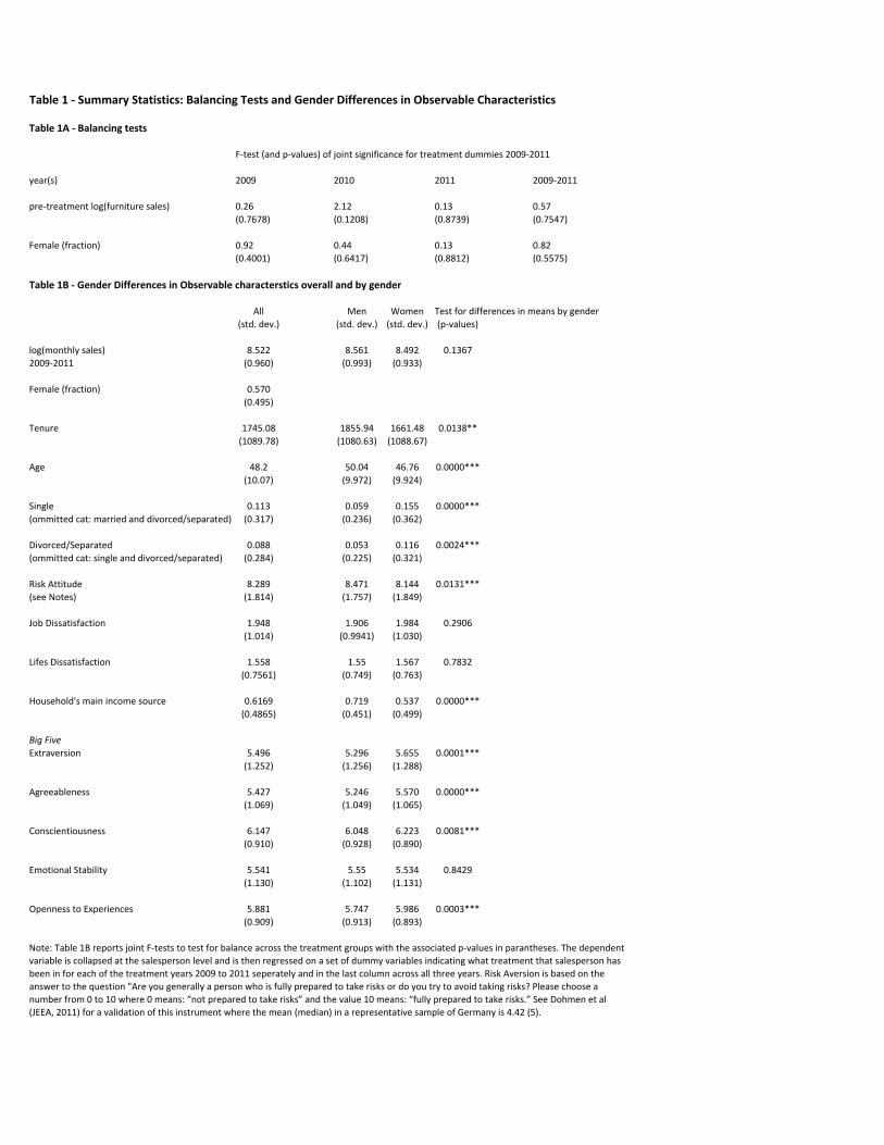
Table  1  -­‐  Summary  Statistics:  Balancing  Tests  and  Gender  Differences  in  Observable  Characteristics

Table  1A  -­‐  Balancing  tests

F-­‐test  (and  p-­‐values)  of  joint  significance  for  treatment  dummies  2009-­‐2011

year(s) 2009 2010 2011 2009-­‐2011

pre-­‐treatment  log(furniture  sales) 0.26 2.12 0.13 0.57(0.7678) (0.1208) (0.8739) (0.7547)

Female  (fraction) 0.92 0.44 0.13 0.82(0.4001) (0.6417) (0.8812) (0.5575)

Table  1B  -­‐  Gender  Differences  in  Observable  characterstics  overall  and  by  gender

All Men Women Test  for  differences  in  means  by  gender  (std.  dev.) (std.  dev.) (std.  dev.) (p-­‐values)

log(monthly  sales) 8.522 8.561 8.492 0.13672009-­‐2011 (0.960) (0.993) (0.933)

Female  (fraction) 0.570(0.495)

Tenure 1745.08 1855.94 1661.48 0.0138**(1089.78) (1080.63) (1088.67)

Age 48.2 50.04 46.76 0.0000***(10.07) (9.972) (9.924)

Single 0.113 0.059 0.155 0.0000***(ommitted  cat:  married  and  divorced/separated) (0.317) (0.236) (0.362)

Divorced/Separated 0.088 0.053 0.116 0.0024***(ommitted  cat:  single  and  divorced/separated) (0.284) (0.225) (0.321)

Risk  Attitude 8.289 8.471 8.144 0.0131***(see  Notes) (1.814) (1.757) (1.849)

Job  Dissatisfaction 1.948 1.906 1.984 0.2906(1.014) (0.9941) (1.030)

Lifes  Dissatisfaction 1.558 1.55 1.567 0.7832(0.7561) (0.749) (0.763)

Household's  main  income  source 0.6169 0.719 0.537 0.0000***(0.4865) (0.451) (0.499)

Big  FiveExtraversion 5.496 5.296 5.655 0.0001***

(1.252) (1.256) (1.288)

Agreeableness 5.427 5.246 5.570 0.0000***(1.069) (1.049) (1.065)

Conscientiousness 6.147 6.048 6.223 0.0081***(0.910) (0.928) (0.890)

Emotional  Stability 5.541 5.55 5.534 0.8429(1.130) (1.102) (1.131)

Openness  to  Experiences 5.881 5.747 5.986 0.0003***(0.909) (0.913) (0.893)

Note:  Table  1B  reports  joint  F-­‐tests  to  test  for  balance  across  the  treatment  groups  with  the  associated  p-­‐values  in  parantheses.  The  dependent  variable  is  collapsed  at  the  salesperson  level  and  is  then  regressed  on  a  set  of  dummy  variables  indicating  what  treatment  that  salesperson  has  been  in  for  each  of  the  treatment  years  2009  to  2011  seperately  and  in  the  last  column  across  all  three  years.  Risk  Aversion  is  based  on  the  answer  to  the  question  "Are  you  generally  a  person  who  is  fully  prepared  to  take  risks  or  do  you  try  to  avoid  taking  risks?  Please  choose  a  number  from  0  to  10  where  0  means:  “not  prepared  to  take  risks”  and  the  value  10  means:  “fully  prepared  to  take  risks.”  See  Dohmen  et  al  (JEEA,  2011)  for  a  validation  of  this  instrument  where  the  mean  (median)  in  a  representative  sample  of  Germany  is  4.42  (5).

Table  2 Natural  log  of  monthly  sales  -­‐  means  and  differences  in  means  by  treatment  groups

Table  2A All  salespeople

Rank No  Rank Differences  in  meansmean  (std.  dev.) mean  (std.  dev.) (robust  standard  errors)

[1] [2] [2]-­‐[1]  =No  Benchmarks mean 8.577 8.778 0.201***

(std.  dev.) (1.021) (0.9494) (0.053)

[3] [4] [4]-­‐[3]  =Benchmarks mean 8.852 8.869 0.017

(std.  dev.) (0.967) (1.046) (0.064)

Differences [3]-­‐[2]  = [3]-­‐[1]  = [4]-­‐[2]  = [4]-­‐[1]  =in  means 0.075 0.276*** 0.091 0.292***

(robust  std.  err.) (0.050) (0.056) (0.062) (0.066)

Table  2B Female  salespeople

Rank No  Rank Differences  in  meansmean  (std.  dev.) mean  (std.  dev.) (robust  standard  errors)

[1'] [2'] [2']-­‐[1']  =No  Benchmarks mean 8.530 8.696 0.166***

(std.  dev.) (0.999) (0.932) (0.068)

[3'] [4'] [4']-­‐[3']  =Benchmarks mean 8.756 8.879 0.123

(std.  dev.) (0.905) (1.017) (0.083)

Differences [3']-­‐[2']  = [3']-­‐[1']  = [4']-­‐[2']  = [4']-­‐[1']  =in  means 0.059 0.226*** 0.182** 0.349***

(robust  std.  err.) (0.064) (0.070) (0.081) (0.086)

Table  2C Male  salespeople

Rank No  Rank Differences  in  meansmean  (std.  dev.) mean  (std.  dev.) (robust  standard  errors)

[1''] [2''] [2'']-­‐[1'']  =No  Benchmarks mean 8.638 8.880 0.242***

(std.  dev.) (1.048) (0.962) (0.084)

[3''] [4''] [4'']-­‐[3'']  =Benchmarks mean 8.972 8.858 -­‐0.114

(std.  dev.) (1.028) (1.081) (0.099)

Differences [3'']-­‐[2'']  = [3'']-­‐[1'']  = [4'']-­‐[2'']  = [4'']-­‐[1'']  =in  means 0.092 0.333*** -­‐0.022 0.220**

(robust  std.  err.) (0.079) (0.089) (0.095) (0.103)

Treatments

Treatments

Treatments

Note:  Tables  contain  weighted  averages  of  the  log  of  monthly  sales  by  treatment  where  the  weights  are  the  number  of  months  a  salesperson  in  a  treatment  had  sales  between  August  2009,  the  start  of  the  experiment,  to  2011.  The  edges  of  the  tables  report  tests  of  differences  in  means  between  treatment  groups  with  robust  standard  errors  in  parantheses.  Salespeople  in  the  "Rank"  treatment  could  see  their  rank  in  terms  of  year-­‐to-­‐date  sales  in  North  America  on  their  personalized  web-­‐report.  Salespeople  in  the  "Benchmark"  treatment  saw  the  year-­‐to-­‐date  sales  in  North  America  required  on  a  given  day  to  be  in  the  top  10%,  25%,  and  50%.  Web-­‐reports  were  updated  daily.

Table  3:  Main  and  Gender  Specific  Treatment  Effects  on  log  of  monthly  sales  by  salespersonDependent  Variable:  Log  or  monthly  salesOmmitted  category:  Rank  Feedback

(1) (2) (3) (4) (5) (6) (7) (8) (9)09-­‐11:  Main  Effect 09-­‐11:  by  Gender 09-­‐11:  Diff-­‐in-­‐Diff 2009:  Main  Effect 2009:  by  Gender 2010:  Main  Effect 2010:  by  Gender 2011:  Main  Effect 2011:  by  Gender

Ommitted  category:   Rank  Feedback Rank  Feedback Rank  Feedback Rank  Feedback Rank  Feedback Rank  Feedback Rank  Feedback No  Rank  Feedback No  Rank  FeedbackNo  Rank  Feedback 0.109** 0.160** 0.117** 0.150* 0.328*** 0.148** 0.173*

(0.0529) (0.0723) (0.0527) (0.0765) (0.117) (0.0668) (0.104)

Female*(No  Rank  Feedback) -­‐0.0965 -­‐0.1470** -­‐0.306** -­‐0.0508(0.0766) (0.0657) (0.132) (0.136)

Gender:  Female -­‐0.0885 (omitted) -­‐0.0895 -­‐0.0900 -­‐0.171*(0.0579) (0.0606) (0.0981) (0.0949)

Rank  Feedback  &  Benchmarks 0.125** 0.203*** 0.0499 0.113* 0.168 0.0532 0.114(0.0582) (0.0779) (0.0611) (0.0676) (0.108) (0.0685) (0.107)

Female*(Rank  Feedback  &  Benchmarks) -­‐0.149* -­‐0.0381 -­‐0.108 -­‐0.110(0.0820) (0.0709) (0.137) (0.138)

Benchmarks  only 0.0637 0.00975 0.0247 -­‐0.0280 -­‐0.123(0.0777) (0.0996) (0.0832) (0.0702) (0.107)

Female*(Benchmarks  only) 0.0911 0.0597 0.171(0.102) (0.0896) (0.142)

Marginal  treatment  effects  for  female  salespeopleNo  Rank  Feedback  (women) 0.0633 -­‐0.0299 0.0216 0.123

(0.0585) (0.0484) (0.0850) (0.0864)

Rank  Feedback  &  Benchmarks  (women) 0.0544 0.0117 0.0597 0.00462(0.0641) (0.0546) (0.0844) (0.0872)

Benchmarks  only  (women) 0.101 0.0844 0.0480(0.0868) (0.0723) (0.0926)

Adjusted  r-­‐squared 0.0455 0.0483 0.2553 0.0393 0.0430 0.0210 0.0229 0.0309 0.0342Month-­‐year  fixed  effects yes yes yes yes yes yes yes yes yesSalespeople  fixed  effects no no yes no no no no no noNumber  of  salespeople  (clusters) 1754 1754 1754 960 960 1285 1285 1434 1434Number  of  observations 29722 29722 29722 7780 7780 10360 10360 11063 11063

Note:  Standard  errors  in  parentheses  clustered  at  the  salesperson  level.  p  <  0.10  (*),  p  <  0.05  (**),  p  <  0.01  (***).  Rank  is  calculated  based  on  year-­‐to-­‐date  sales  in  North  America.  "No  Rank  Feeback"  provides  neither  rank  nor  benchmarks,  Benchmarks  is  the  treatment  where  we  showed  salespeople  what  it  currently  takes  to  be  in  the  top  10%,  25%,  and  50%  in  North  America.

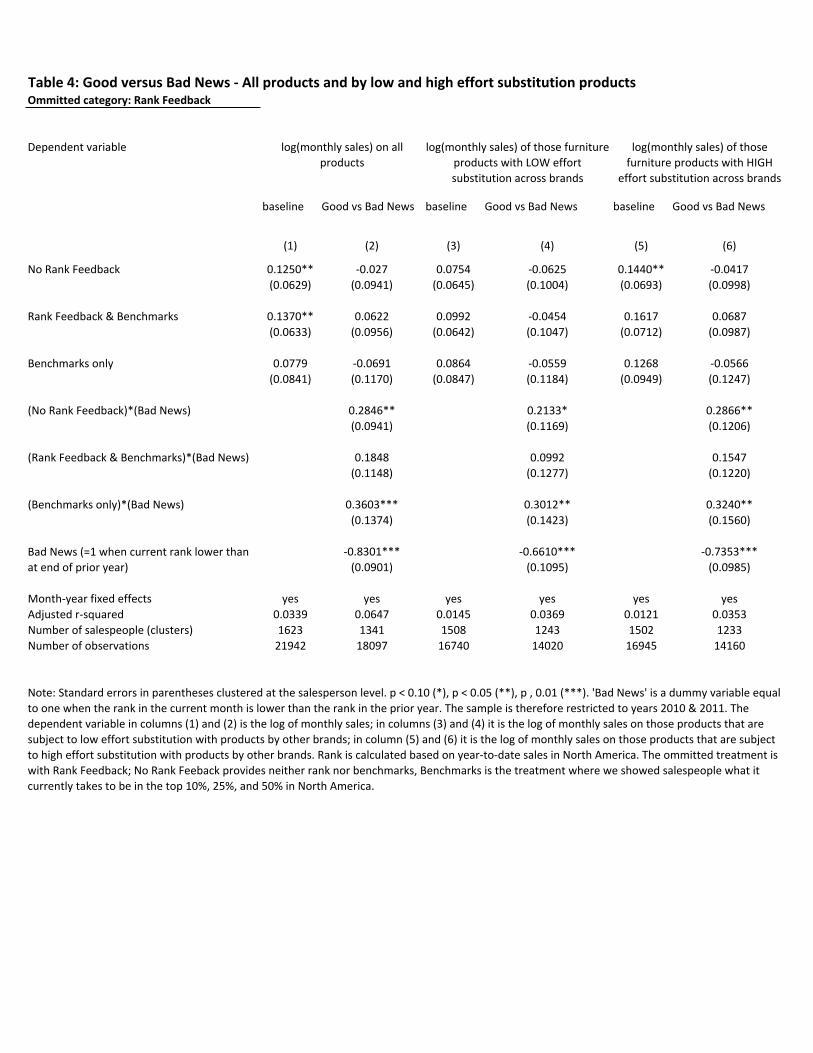
Table  4:  Good  versus  Bad  News  -­‐  All  products  and  by  low  and  high  effort  substitution  productsOmmitted  category:  Rank  Feedback

Dependent  variable

baseline Good  vs  Bad  News baseline Good  vs  Bad  News baseline Good  vs  Bad  News

(1) (2) (3) (4) (5) (6)

No  Rank  Feedback 0.1250** -­‐0.027 0.0754 -­‐0.0625 0.1440** -­‐0.0417(0.0629) (0.0941) (0.0645) (0.1004) (0.0693) (0.0998)

Rank  Feedback  &  Benchmarks 0.1370** 0.0622 0.0992 -­‐0.0454 0.1617 0.0687(0.0633) (0.0956) (0.0642) (0.1047) (0.0712) (0.0987)

Benchmarks  only 0.0779 -­‐0.0691 0.0864 -­‐0.0559 0.1268 -­‐0.0566(0.0841) (0.1170) (0.0847) (0.1184) (0.0949) (0.1247)

(No  Rank  Feedback)*(Bad  News) 0.2846** 0.2133* 0.2866**(0.0941) (0.1169) (0.1206)

(Rank  Feedback  &  Benchmarks)*(Bad  News) 0.1848 0.0992 0.1547(0.1148) (0.1277) (0.1220)

(Benchmarks  only)*(Bad  News) 0.3603*** 0.3012** 0.3240**(0.1374) (0.1423) (0.1560)

-­‐0.8301*** -­‐0.6610*** -­‐0.7353***(0.0901) (0.1095) (0.0985)

Month-­‐year  fixed  effects yes yes yes yes yes yesAdjusted  r-­‐squared 0.0339 0.0647 0.0145 0.0369 0.0121 0.0353Number  of  salespeople  (clusters) 1623 1341 1508 1243 1502 1233Number  of  observations 21942 18097 16740 14020 16945 14160

log(monthly  sales)  of  those  furniture  products  with  LOW  effort  substitution  across  brands

log(monthly  sales)  of  those  furniture  products  with  HIGH  

effort  substitution  across  brands

log(monthly  sales)  on  all  products

Note:  Standard  errors  in  parentheses  clustered  at  the  salesperson  level.  p  <  0.10  (*),  p  <  0.05  (**),  p  ,  0.01  (***).  'Bad  News'  is  a  dummy  variable  equal  to  one  when  the  rank  in  the  current  month  is  lower  than  the  rank  in  the  prior  year.  The  sample  is  therefore  restricted  to  years  2010  &  2011.  The  dependent  variable  in  columns  (1)  and  (2)  is  the  log  of  monthly  sales;  in  columns  (3)  and  (4)  it  is  the  log  of  monthly  sales  on  those  products  that  are  subject  to  low  effort  substitution  with  products  by  other  brands;  in  column  (5)  and  (6)  it  is  the  log  of  monthly  sales  on  those  products  that  are  subject  to  high  effort  substitution  with  products  by  other  brands.  Rank  is  calculated  based  on  year-­‐to-­‐date  sales  in  North  America.  The  ommitted  treatment  is  with  Rank  Feedback;  No  Rank  Feeback  provides  neither  rank  nor  benchmarks,  Benchmarks  is  the  treatment  where  we  showed  salespeople  what  it  currently  takes  to  be  in  the  top  10%,  25%,  and  50%  in  North  America.

Bad  News  (=1  when  current  rank  lower  than  at  end  of  prior  year)

<-- pilot phase -->

1st randomization

2nd randomization

3rd randomization

88.

59

9.5

1010

.5

Log

of a

vera

ge m

onth

ly s

ales

Jan '09 Aug '09 Jan '10 Jul '10 Jan '11 Jul '11 Dec '11

no rank feedback benchmarksrank feedback & benchmarks rank feedback

Figure 1 - Average monthly sales by treatment: all salespeople

<-- pilot phase -->

1st randomization

2nd randomization

3rd randomization

88.

59

9.5

1010

.5

Log

of a

vera

ge m

onth

ly s

ales

Jan '09 Aug '09 Jan '10 Jul '10 Jan '11 Jul '11 Dec '11

no rank feedback (fem.) benchmarks (fem.)rank feedback & benchmarks (fem.) rank feedback (fem.)

Figure 2 - Average monthly sales by treatment: female salespeople

<-- pilot phase -->

1st randomization

2nd randomization

3rd randomization

88.

59

9.5

1010

.5

Log

of a

vera

ge m

onth

ly s

ales

Jan '09 Aug '09 Jan '10 Jul '10 Jan '11 Jul '11 Dec '11

no rank feedback (male) benchmarks (male)rank feedback & benchmarks (male) rank feedback (male)

Figure 3 - Average monthly sales by treatment: male salespeople

Table  A1 Natural  log  of  monthly  sales  -­‐  means  and  differences  in  means  by  year  and  treatment  groups

Table  A1b All  salespeople

No  Rank Differences  in  meansmean  (std.  dev.) (robust  standard  errors)

[1] [2] [3] [4] [5] [3]-­‐[1]= [4]-­‐[2]=year Aug-­‐Dec  2009 2010 Aug-­‐Dec  2009 2010 2011 Aug-­‐Dec  09 2010mean 8.403 8.681 8.566 8.834 8.866 0.1637* 0.1535**

(std.  dev.) (1.2743) (0.9252) (1.124) (0.927) (0.987) (0.093) (0.068)

[6] [7] [8] [8]-­‐[7]=year 2010 2011 2011 2011mean 8.801 8.937 8.844 -­‐0.093

(std.  dev.) (0.9321) (1.027) (1.072) (0.073)

[6]-­‐[4]= [7]-­‐[5]= [6]-­‐[2]= [8]-­‐[5]=year 2010 2011 2010 2011

Diff.  in  means -­‐0.033 0.071 0.1203* -­‐0.0219(robust  std.  err.) (0.068) (0.070) (0.069) (0.072)

Table  A1c Female  salespeople

No  Rank Differences  in  meansmean  (std.  dev.) (robust  standard  errors)

[1'] [2'] [3'] [4'] [5'] [3']-­‐[1']= [4']-­‐[2']=year Aug-­‐Dec  2009 2010 Aug-­‐Dec  2009 2010 2011 Aug-­‐Dec  09 2010mean 8.320 8.640 8.404 8.769 8.787 0.084 0.129

(std.  dev.) (1.307) (0.864) (1.045) (0.927) (0.972) (0.122) (0.087)

[6'] [7'] [8'] [8']-­‐[7']=year 2010 2011 2011 2011mean 8.709 8.809 8.850 0.042

(std.  dev.) (0.872) (0.945) (1.041) (0.093)

[6']-­‐[4']= [7']-­‐[5']= [6']-­‐[2']= [8']-­‐[5']=year 2010 2011 2010 2011

Diff.  in  means -­‐0.060 0.021 0.069 0.063(robust  std.  err.) (0.088) (0.089) (0.085) (0.095)

Table  A1d Male  Salespeople

No  Rank Differences  in  meansmean  (std.  dev.) (robust  standard  errors)

[1''] [2''] [3''] [4''] [5''] [3'']-­‐[1'']= [4'']-­‐[2'']=year Aug-­‐Dec  2009 2010 Aug-­‐Dec  2009 2010 2011 Aug-­‐Dec  09 2010mean 8.509 8.732 8.784 8.91 8.965 0.275* 0.178*

(std.  dev.) (1.226) (0.996) (1.192) (0.923) (1.000) (0.143) (0.106)

[6''] [7''] [8''] [8'']-­‐[7'']=year 2010 2011 2011 -­‐0.260**mean 8.905 9.097 8.837 (0.115)

(std.  dev.) (0.987) (1.103) (1.041)

[6'']-­‐[4'']= [7'']-­‐[5'']= [6'']-­‐[2'']= [8'']-­‐[5'']=year 2010 2011 2010 2011

Diff.  in  means -­‐0.005 0.132 0.172 -­‐0.128(robust  std.  err.) (0.103) (0.109) (0.110) (0.110)

Rankmean  (std.  dev.)

Note:  Tables  contain  weighted  averages  of  the  log  of  monthly  sales  by  treatment  and  year  where  the  weights  are  the  number  of  months  a  salesperson  in  a  treatment  had  sales  in  the  years  2009  to  2011.  The  edges  of  the  tables  report  tests  of  differences  in  means  between  treatment  groups  with  robust  standard  errors  in  parantheses.  Salespeople  in  the  "Rank"  treatment  could  see  their  rank  in  terms  of  year-­‐to-­‐date  sales  in  North  America  on  their  personalized  web-­‐report.  Salespeople  in  the  "Benchmark"  treatment  saw  the  year-­‐to-­‐date  sales  in  North  America  required  on  a  given  day  to  be  in  the  top  10%,  25%,  and  50%.  Web-­‐reports  were  updated  daily.  The  "year"  rows  shows  which  treatments  were  in  place  in  a  what  year.  Salespeople  were  randomly  allocated  to  treatment  groups  in  August  2009,  January  2010,  and  January  2011  and  the  randomization  occured  for  all  salespeople  at  each  of  these  dates  so  that  treatment  groups  memberships  were  uncorrelated  across  year.  

No  Benchmarks

No  Benchmarks

Benchmarks

Benchmarks

Treatments

Treatments

Treatments

mean  (std.  dev.)

No  Benchmarks

Benchmarks

Rankmean  (std.  dev.)

Rank

Table  A2:  Main  and  Gender  Specific  Quantile  Treatment  Effects

Dependent  Variable:  log  of  sales  by  month  and  salespersonOmmitted  category:  Rank  Feedback

All  Salespeople (1) (2) (3) (4) (5)Quantile q10 q25 q50 q75 q90No  Rank  Feedback 0.159** 0.141*** 0.121*** 0.152*** 0.0709

(0.0622) (0.0489) (0.0387) (0.0368) (0.0442)

Rank  Feedback  &  Benchmarks 0.131* 0.130** 0.124*** 0.161*** 0.177***(0.0683) (0.0518) (0.0395) (0.0368) (0.0485)

Benchmarks  only 0.114 0.0727 0.0558 0.114** 0.124**(0.0800) (0.0615) (0.0490) (0.0524) (0.0588)

Period  fixed  effects yes yes yes yes yesN 29722 29722 29722 29722 29722

Female  SalespeopleQuantile q10 q25 q50 q75 q90No  Rank  Feedback 0.0983 0.0813 0.108** 0.102* 0.0317

(0.0770) (0.0628) (0.0532) (0.0521) (0.0571)

Rank  Feedback  &  Benchmarks 0.0750 0.0493 0.0769 0.0745 0.0618(0.0846) (0.0672) (0.0594) (0.0542) (0.0664)

Benchmarks  only 0.147 0.0719 0.168** 0.149** 0.160**(0.105) (0.0871) (0.0740) (0.0760) (0.0791)

Period  fixed  effects yes yes yes yes yesN 16177 16177 16177 16177 16177

Male  SalespeopleQuantile q10 q25 q50 q75 q90No  Rank  Feedback 0.249** 0.196*** 0.105 0.171*** 0.0429

(0.0979) (0.0739) (0.0643) (0.0597) (0.0679)

Rank  Feedback  &  Benchmarks 0.256** 0.251*** 0.132* 0.266*** 0.245***(0.0994) (0.0803) (0.0681) (0.0652) (0.0746)

Benchmarks  only 0.125 0.0234 -­‐0.135* 0.0465 0.0298(0.131) (0.100) (0.0817) (0.0835) (0.0921)

Period  fixed  effects yes yes yes yes yesN 13545 13545 13545 13545 13545

Note:  Quantile  regressions  with  robust  standard  errors  based  on  5000  replications.

Table  A3  Treatment  Effects  by  Observable  CharactersisticsDependent  Variable:  Log  or  monthly  salesOmmitted  category:  Rank  Feedback

(1) (2) (3) (4) (5) (6) (7) (8) (9) (10) (11) (12)Interaction  variable  (INTVAR) Age Single Divorced Risk  Attitudes Main  Household  Income  SourceJob-­‐Dissatisfaction Life-­‐Dissatisfaction Extravertedness Agreeableness Conscientiousness

No  Rank  Feedback 0.379* 0.150 0.161 -­‐0.0534 0.213* 0.129 0.0788 -­‐0.0164 0.483* -­‐0.0861 0.0736 0.208(0.229) (0.102) (0.102) (0.266) (0.122) (0.150) (0.149) (0.264) (0.291) (0.377) (0.260) (0.336)

Rank  &  Benchmarks 0.779*** 0.238** 0.250** 0.442* 0.331** 0.251 0.175 0.159 0.570* -­‐0.330 0.625** 0.321(0.272) (0.111) (0.111) (0.264) (0.135) (0.158) (0.161) (0.257) (0.304) (0.418) (0.273) (0.361)

Benchmarks 0.384 -­‐0.106 -­‐0.0894 -­‐0.537 -­‐0.231 -­‐0.215 -­‐0.275 -­‐0.599* -­‐0.179 -­‐0.406 0.00877 -­‐0.593(0.311) (0.141) (0.140) (0.350) (0.160) (0.190) (0.193) (0.329) (0.400) (0.502) (0.393) (0.485)

Female*(No  Rank  Feedback) -­‐0.131 -­‐0.148 -­‐0.150 -­‐0.145 -­‐0.163 -­‐0.163 -­‐0.153 -­‐0.158 -­‐0.132 -­‐0.153 -­‐0.150 -­‐0.148(0.0909) (0.106) (0.104) (0.104) (0.103) (0.104) (0.104) (0.103) (0.106) (0.104) (0.104) (0.104)

Female*(Rank  &  Benchmarks) -­‐0.166* -­‐0.191* -­‐0.214* -­‐0.225** -­‐0.236** -­‐0.212* -­‐0.227** -­‐0.217* -­‐0.186* -­‐0.239** -­‐0.219* -­‐0.213*(0.0998) (0.114) (0.114) (0.113) (0.114) (0.112) (0.112) (0.113) (0.112) (0.115) (0.113) (0.114)

Female*Benchmarks 0.151 0.168 0.141 0.237* 0.195 0.190 0.191 0.134 0.184 0.162 0.186 0.171(0.120) (0.143) (0.143) (0.141) (0.141) (0.142) (0.141) (0.145) (0.141) (0.145) (0.141) (0.145)

Female -­‐0.110 -­‐0.0549 -­‐0.0780 -­‐0.0589 -­‐0.0548 -­‐0.0690 -­‐0.0712 -­‐0.0847 -­‐0.0695 -­‐0.0778 -­‐0.0688 -­‐0.0748(0.0720) (0.0811) (0.0820) (0.0812) (0.0816) (0.0808) (0.0801) (0.0799) (0.0800) (0.0812) (0.0814) (0.0813)

Interaction  Variable  (INTVAR) -­‐0.00240 -­‐0.264** 0.0588 0.0339 0.0881 -­‐0.102*** -­‐0.176*** 0.0334 -­‐0.00745 0.0346 0.0459 0.0132(0.00359) (0.116) (0.133) (0.0224) (0.0829) (0.0390) (0.0588) (0.0351) (0.0394) (0.0499) (0.0344) (0.0438)

INTVAR*(Nor  Rank  Feedback) -­‐0.00407 0.0756 0.0271 0.0257 -­‐0.0659 0.0188 0.0594 0.0327 -­‐0.0621 0.0398 0.0159 -­‐0.00821(0.00450) (0.145) (0.176) (0.0295) (0.103) (0.0554) (0.0723) (0.0437) (0.0515) (0.0599) (0.0429) (0.0547)

INTVAR*(Rank  &  Benchmarks) -­‐0.0118** -­‐0.103 0.0222 -­‐0.0217 -­‐0.105 0.00193 0.0618 0.0174 -­‐0.0632 0.0962 -­‐0.0672 -­‐0.0121(0.00508) (0.184) (0.186) (0.0291) (0.113) (0.0545) (0.0705) (0.0445) (0.0523) (0.0667) (0.0446) (0.0592)

INTVAR*Benchmarks -­‐0.00826 0.169 0.287 0.0517 0.232* 0.0700 0.127 0.0993* 0.0163 0.0538 -­‐0.0167 0.0873(0.00590) (0.212) (0.219) (0.0382) (0.137) (0.0651) (0.104) (0.0583) (0.0685) (0.0811) (0.0668) (0.0815)

Joint  test  H0:  INTVAR=0,  INTVAR*(Nor  Rank  Feedback)=0,  INTVAR*(Rank  &  Benchmarks)=0,  INTVAR*Benchmarks=0F-­‐statistic 3.824** 2.085* 0.533 1.869* 1.221 3.918*** 3.553*** 1.619 1.373 1.492 1.012 0.302p-­‐value 0.00194 0.0653 0.751 0.0975 0.297 0.00163 0.00349 0.152 0.232 0.190 0.409 0.912Joint  test  H0:  Female=0,  Female*(Nor  Rank  Feedback)=0,  Female*(Rank  &  Benchmarks)=0,  Female*Benchmarks=0F-­‐statistic 3.480*** 2.216* 2.667** 2.819** 2.845** 2.925** 2.938** 2.787** 2.367** 2.995** 2.758** 2.701**p-­‐value 0.00399 0.0510 0.0212 0.0156 0.0148 0.0126 0.0123 0.0167 0.0381 0.0110 0.0177 0.0198

Adjusted  r-­‐squared 0.0457 0.0463 0.0448 0.0471 0.0457 0.0475 0.0474 0.0468 0.0457 0.0465 0.0452 0.0446Number  of  salespeople  (clusters) 1043 770 770 771 770 771 771 771 771 771 771 771Number  of  observations 21430 16508 16508 16530 16508 16530 16530 16530 16530 16530 16530 16530Notes:  Standard  errors  in  parantheses,  *  p<0.10,  **  p<0.05,  ***  p<0.01.  Errors  clustered  at  the  salesperson  level.  The  dependent  variable  in  all  regressions  is  the  log  of  monthly  sales.  Each  column  uses  a  difference  variables  as  interaction  terms.  In  column  (1)  the  interaction  variable  is  gender,  in  column  (2)  it  is  age,  etc.  The  regression  also  includes  a  constant  and  a  dummy  for  a  treament  only  used  during  the  pilot  phase  in  2009  where  we  provided  normalized  rank  feedback  in  one  treatment  arm.  See  Table  1  for  definition  of  variables

Emotional  Stabilty

Opennness  to  New  Experiences

No Rank Feedback Rank & Benchmarks

Benchmarks

-.4-.2

0.2

.4

0 20 40 60 80 100

No Rank Feedback Rank & Benchmarks

Benchmarks

-1-.5

0.5

0 20 40 60 80 100

No Rank Feedback Rank & Benchmarks

Benchmarks

-.4-.2

0.2

.4

0 20 40 60 80 100