Raw Data Compression in Computed Tomography:Noise Shaping

Yao Xie(team member: Adam Wang)

Project Final Report for EE372Stanford University, Spring 2006-07

July 18, 2007

Abstract

1 Introduction

1.1 Background

X-ray computed tomography (CT) builds on the physical principles of radiography. It usesmultiple views of an external x-ray source and images x-ray attenuation properties µ as afunction of location within the body.

In a CT scanner, large amounts of raw data are collected in the rotating gantry andmust be transferred offline for processing and image reconstruction. Generally this transferis made through a slip ring that has a limited data transfer rate. Compression can be usedto reduce the data rate through the slip ring, but one needs to ensure that the compressiondoes not degrade image quality.

This problem becomes more severe in the new inverse geometry CT (IGCT) system[GRGJ04][SFP05]. Because IGCT has multiple sources, it requires higher data rate thanthat of a typical cone beam CT system, which is already quite heavy. Consider a typicalcone beam geometry CT system whose data transmission rate can be estimated as: 984views/rotation × 888 detectors/row × 64 rows × 3.33 rotation/s × 16 bits/detector ≈ 400MB/s.

However, our preliminary literature search has shown that no one has considered com-pressing data before transmitting it through the slip ring, and the only work that has beendone on compressing raw data (sinogram) has used standard image compression techniquessuch as JPEG [BW01]. These techniques do not take into account the nature of the sinogramand how errors in the sinogram contribute to errors (noise) in the reconstructed image.

1

Figure 1: A fan beam CT system.

Compression can be applied not only to raw data transmission, but also to raw datastorage. Currently, only reconstructed images are stored in PACS (picture archiving andcommunication system). This does not allow the flexibility to reconstruct different slices ordo planar reformats since the original raw data is discarded. If we are able to compress thesinogram data with a tolerable amount of loss in the reconstructed image quality, we canstore the raw data and then reconstruct desired images in the future.

1.2 Raw Data Model

To form images in CT systems, a set of x-ray beams are scanned through the entire field ofview (where the object lies) in what is known as fan or, more generally, cone beam geometry.We will consider 2-D scan with fan beam geometry, as shown in Fig. 11. Each x-ray beam(measured by the nth detector), is modelled as a line positioned at rn with orientation θi.The attenuation values µ(x, y) along the path of the x-ray beam are superimposed, resultingin a line-integral of the attenuation. The attenuated x-ray beam intensities are measuredusing detectors. The expected value of the measured intensity for a particular beam is givenby Beer’s law:

I(rn, θi) = I0 exp

{−

∫

l(rn,θi)µ(x, y)dl

},

1www.medcyclopaedia.com

2

where I0 is the incident intensity of the x-ray beam passing through the object, and l(rn, θi)is the line through which the x-ray passing through the object.

This process is repeated for a large number of angles, yielding line attenuation samples ofall angles θi, i = 0, · · · , Nθ − 1 and of all distances rn, n = 0, · · · , Nr − 1 from the centerof the detector array within the field of view (FOV). Then we have a complete data set of{gθi

(rn)}. Due to the discrete nature of the x-ray photon, each measurement gθi(rn) follows

a Poisson distribution with mean and variance I(rn, θi).The sinogram is a two-dimensional representation of the measured signal {gθi

(rn)}. Wealso refer to the sinogram as the raw data. From the sinogram, the actual attenuation ateach voxel of the scanned slice can be reconstructed [DeM01]. Before image reconstruction,the raw data is often normalized by I0 and followed by a logarithmic operation:

− log

(gθi

(rn)

I0

)=

∫

l(rn,θi)µ(x, y)dl.

This logarithmic operation essentially corresponds to a logarithmic compander before quan-tization, which is widely used for A/D conversion. The logarithmic compander effectivelyreduces the data dynamic range. In addition to the logarithmic compander, we can alsoconsider other companders such a square root compander (as studied in Adam’s projectreport). In this project we only use the logarithmic compander.

1.3 Project Goal

In our project, we will consider quantization and fixed rate lossy compression for CT imag-ing raw data (sinogram). We will design our quantizer considering the data properties ofsinograms.

Our problem can be explained by the block diagram in Fig. 2. We will compress theraw data, and then the raw data is reconstructed to form the image {µ(x, y)}, and ourultimate goal is to keep the maximum difference between the image reconstructed from thecompressed and from the uncompressed raw data to be “visibly indistinguishable.”

Typically, the reconstructed images are displayed in integer units of Houndsfield Units(HU) [DeM01], from -1000 to +3000, so errors that we introduce from compression of ±1 HUare within the contrast resolution capability of CT systems. Therefore, when we subtract thereconstructed compressed image from the original reconstructed image, if the peak differenceis within ±1 HU, then “no one will complain.” Thus our distortion measure is defined interms of this difference image.

However, if we use a distortion measure in the reconstructed image space, since the imagereconstruction process is not spatial invariant, it is not a convenient distortion measure forLloyd types of iterative algorithms (for each quantizer, we have to reconstruct the image, findout the distortion, and go back and forth.) To solve this problem, we study the relationshipbetween the quantization errors in the sinogram space with the errors in the reconstructedimage, and introduce a frequency weighted distortion measure in the sinogram space. Thesecond distortion measure directly relates the quantized data with raw data.

3

Figure 2: Block diagram of CT raw data quantization/compression model.

4

The contributions of this project are: 1) study a distortion measure that relates the rawdata space to the reconstructed image; 2) without changing rate, we consider two approachesto achieve a lower noise level due to quantization in the center region of the reconstructedimage: first, noise shaping, and second, sub-band coding using DFT and bit-loading.

2 Quantizer Model

We will consider a scalar uniform quantizer with bin width ∆ and N levels. In our projectwe will use 8 to 10 bits for CT data compression, which corresponds to a minimum numberof quantizer levels of N = 28. Under these high rate and small distortion assumptions, wecan use the high rate Bennett’s approximation [Gra07], and model the quantizer error asadditive white process uncorrelated with each other and uncorrelated with the quantizeroutput. The quantizer model is given by:

gθi(rn) = gθi

(rn) + eθi(rn), n = 1, · · · , Nr, i = 1, · · · , Nθ.

where gθi(rn) is the quantizer output and eθi

(rn) is the quantizer error.Under the high rate assumptions, the quantizer error eθi

(rn) follows the uniform distri-bution in [−∆/2, ∆/2], with mean 0 and variance ∆2/12.

3 Distortion Measure

3.1 Quantization Error Frequency Property Study

We found that the low frequency band of the quantization errors contributes to the centerof the reconstructed image, and the high frequency band error contributes more to theperipheral region of the image. (In fact, noise in different detectors will also contribute todifferent parts in the image, as studied in Adam’s project report. In this report, we willexplore the frequency property of quantization error.)

To study the quantizer noise distribution property, we created a thorax phantom asshown in Fig. 3, and simulated the CT data using CatSim [DBC+07], a GE proprietarypackage developed for the express purpose of simulating various CT configurations. In fact,without such simulation software, raw data is exceedingly difficult to acquire since all of theprocessing to produce the final reconstructed image is “hidden away” within a commercialsystem. The image reconstruction block is also implemented using CatSim. The so-obtainedCT raw data are represented with 32 bit floating point accuracy.

To study the effects of different frequency components of the quantization errors in thereconstructed image, we performed the following experiment. We added three frequencybanded (with equal total bandwidth) noise signals to the 1D DFT of the uncompressedsinogram (32 bits floating point) in the view direction (as opposed to 2D DFT). The noise isuniformly distributed in [−∆/2, ∆/2], and the total power is about the same in these threefrequency bands. We find the dynamic range of the raw data to be [Umin, Umax], and thenuse an 8-bit uniform scalar quantizer, with ∆ = Umax−Umin

28 .

5

100 200 300 400 500

50

100

150

200

250

300

350

400

450

500

0

0.1

0.2

0.3

0.4

0.5

0.6

Figure 3: Reconstructed image for the thorax phantom, using raw data (32 bit floatingpoint).

The frequency banded noises are shown in Fig. 4(a), Fig. 4(b) and Fig. 4(c). The resultednoisy sinograms are then reconstructed, and the difference images using the quantized andunquantized data are then found, as shown in in Fig. 4(b), Fig. 4(d), and Fig. 4(e). Wecan clearly see that the high frequency noise has less error in the center of the reconstructedimage, whereas the low frequency noise has almost uniform noise throughout the image. Fig.5(a) shows the absolute peak value (in the unit cm−1) in the difference image, as a functionof distance di from the center of the image.

3.2 Distortion Measure

In many clinical applications, the center of the image contains the object of interest. Sowe would like to keep the error due to quantization/compression small in the center of theimage, and allow a large error in the peripheral region of the image. For these reasons, wedefine the following distortion measure in the image space:

DI =1

Np

Np−1∑

i=0

α2(di)ε2i ,

6

200 400 600 800

200

400

600

800

Difference Image, Low frequence noise

100 200 300 400 500

50

100

150

200

250

300

350

400

450

500−0.01

−0.008

−0.006

−0.004

−0.002

0

0.002

0.004

0.006

0.008

0.01

(a): Low band frequency band noise, (b): Difference image, adding (a),

200 400 600 800

200

400

600

800

Difference Image, band frequence noise

100 200 300 400 500

50

100

150

200

250

300

350

400

450

500

−0.01

−0.005

0

0.005

0.01

(c): Mid band frequency band, (d): Difference image, adding (c)

200 400 600 800

200

400

600

800

Difference Image, high frequence noise

100 200 300 400 500

50

100

150

200

250

300

350

400

450

500−3

−2

−1

0

1

2

3

4x 10−3

(e): High band frequency, (f): Difference image, adding (e).

Figure 4: Different band frequency noise (used to modelling the quantizer error),added to DFT of the sinogram, and their corresponding difference images.

7

0 50 100 150 200 2500

0.002

0.004

0.006

0.008

0.01

0.012

0.014

Distance from centre of image

Pea

k A

bsol

ute

Err

or

Low freq noiseMidband freq noiseHigh freq noise

Figure 5: (a): peak error versus distance from the center of the image (pixels).

where Np is the number of pixels,

εi = maxx2+y2=d2

i

|µ(x, y)− µ(x, y)|

is the peak error in the difference image (with distance di from the center of the image), andweights {α2

i } are inversely proportional to distances with

α2i ∝ 1/d2

i ,∑

i

α2i = 1.

However, this distortion measure DI is not easy to handle because it is not directly relatedto the raw sinogram data. From our study, we found that high frequency noise contributesto the peripheral region, whereas the low frequency noise contributes to the center of thereconstructed image. For this consideration, we can define a frequency weighted distortionmeasure. If we denote by capital letters the components of the discrete Fourier transform(DFT) of a signal, then in the frequency domain, the weighted MSE is given by:

DS =1

NθNd

Nθ−1∑

j=0

β2j

Nd−1∑

n=0

|Gn(fj)−Gn(fj)|2 =1

NθNd

Nθ−1∑

j=0

β2j

Nd−1∑

n=0

|En(fj)|2.

The weights {βj} are inversely proportional to frequency of the noise:

β2j ∝ 1/f2

j ,∑

β2j = 1.

Here we let β0 = 1. This distortion directly measures the distortion in the sinogram spacedue to quantization and compression. Note that it is similar to the (relate to the Itakura

8

0 0.05 0.1 0.151

1.5

2

2.5

3

3.5x 10

−8

DS

DI

Figure 6: Di versus Df , in Figs. 4(b), 4(d), and 4(f).

distortion measure [Ita75]) It can be used as a distortion measure for quantization, such asin the Lloyd algorithm [Gra07].

Then we measure the two distortions, DS and DI , for these three cases as shown in Fig.6(b). Although we only have three points, we can see these two distortion measures arepositively correlated. In the following, as a heuristic, we can minimize DS to achieve thegoal of minimizing DI (because DS is under the control of the quantizer, whereas DI isaffected by image reconstruction algorithm).

4 Error Diffusion Coding

4.1 Error Feedback Quantization

Our motivation for error feedback quantization is to ensure that the quantization error doesnot accumulate in the reconstructed image. We find that it is related to the early work oferror diffusion code [Ana89]. However, we come to our algorithm from a different perspective.

To simplify our analysis, we consider the parallel beam CT image reconstruction algo-rithm (which is a good approximation to the fan-beam reconstruction algorithm in mostcases). The parallel beam reconstruction algorithm forms the reconstructed image by back-projecting all the filtered rays, as shown in Fig. 72:

µ(x, y) =Nr−1∑

i=0

Nθ−1∑

j=0

(gθj

(ri) ∗ c(ri))δ(x cos θj + y sin θj − ri),

2Courtesy: www.dspguide.com

9

Figure 7: Back projection for parallel beam geometry.

the backprojection filer c(ri) can be well approximated by a delta function δ(·). Then thereconstructed pixel value is simply determined by summing all the projection ray passingthrough that pixel.

Our error feedback quantization method is given by (for notational simplicity, we dropthe dependence of variables on rn):

• Set eθ1 = 0;

• For each reading gθi

g′θi= gθi

+ eθi−1;

gθi= E(g′θi

) (the codeword to be transmitted);

eθi= g′θi

−D(gθi)

where E is the encoder and D is the decoder. We note that this scheme is related to errordiffusion coding with a particular noise shaping filter [Ana89].

The quantization error will not accumulate in the reconstructed image in this way. Asan example, we consider the pixel at the center of the image, whose value is determined bythe sum of all the measurements from the center detector. Consider all Nθ measurementsmade by the center detector, and recall that compression introduces a zero mean error with

10

an RMS value of ∆2/12. If the error is independent for each of the Nθ readings, the sumof the Nθ readings will have an RMS value (DC error) of

√Nθ∆

2/12. However, using ourproposed scheme, the RMS value of the sum will reduce to ∆2/12 (see Appendix A for moredetailed explanation).

This can also be interpreted from the frequency domain perspective. Indeed, the processof feeding the error due to compression into another reading will reduce the low temporalfrequency components of the noise. If we consider the z-transform of all the quantities inFig. 8(a), we have the z transform of the quantization error

En(z) = Gn(z)− Un(z) = Gn(z)−Gn(z) + z−1H(z)E(z) = En(z).

And in our error feedback system, as shown in Fig. 8(a), H(z) = 1. Hence, the quantizationerror en(i) = gn(i)− gn(i) is related to the quantizer error en(i) = gn(i)− un(i) by

H(z) =En(z)

En(z)= 1 + z−1H(z).

The filter H(z) has one zero at z = −1, hence creates a high-pass filter, whose frequencyresponse is given in Fig. 10(a). Then the quantization error is a filtered version of thequantizer error. If the quantizer error is assumed to be an independent white noise sequencein the linearized model then the noise shaping is achieved by properly choosing H(z).

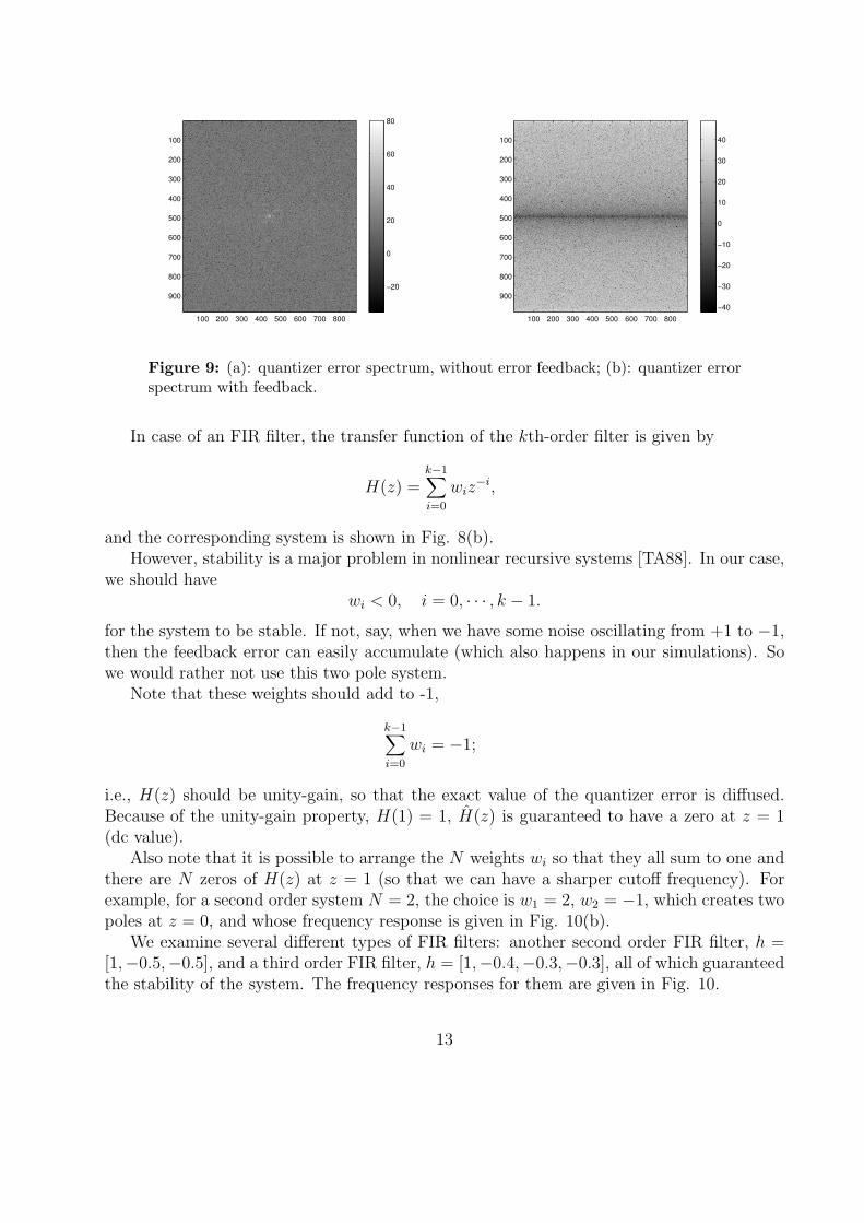
We apply this simple error feedback quantizer to the thorax phantom raw data in Fig. 3,reconstruct the image and find the difference image. Fig. 9(b) gives the spectrum of the noise(pixel value of the difference image). Note that when compared with the noise spectrum ofthe linear scalar quantizer without feedback in Fig. 8(a), the error feedback system passesthe error through a high pass filter and achieves a desired noise spectrum shape.

Note that herein we only perform error feedback for each detector independently. We canalso consider feeding errors across different detectors, however, it is not yet clear to us howthis will benefit the final image reconstruction. Also, implementing error feedback online foreach detector independently is easier in the CT gantry hardware.

We may also consider feeding errors for a single view (independent of other views) acrossall the detectors. However, our preliminary simulation results have shown that this schemewill create more noise in the center region of the reconstructed image than the peripheralregion. One possible explanation for this is that, in the image reconstruction algorithm, wehave applied a high pass ramp filter across detector measurements, for each view. The imagereconstruction ramp filter will counteract the efforts of our noise shaping filter, so we willnot consider this type of error feedback.

4.2 Error feedback filter comparison

A more general case to the first order error feedback system in Fig. 8(a), is to design thefilter H(z) to achieve our desired noise spectrum. Particularly, we would like to push thequantizer noise power to the high frequency region as much as possible.

11

Figure 8: Block diagram for the error feedback schemes: (a): our error feedbackscheme is a first order system; (b): general error feedback scheme.

12

100 200 300 400 500 600 700 800

100

200

300

400

500

600

700

800

900−20

0

20

40

60

80

100 200 300 400 500 600 700 800

100

200

300

400

500

600

700

800

900−40

−30

−20

−10

0

10

20

30

40

Figure 9: (a): quantizer error spectrum, without error feedback; (b): quantizer errorspectrum with feedback.

In case of an FIR filter, the transfer function of the kth-order filter is given by

H(z) =k−1∑

i=0

wiz−i,

and the corresponding system is shown in Fig. 8(b).However, stability is a major problem in nonlinear recursive systems [TA88]. In our case,

we should havewi < 0, i = 0, · · · , k − 1.

for the system to be stable. If not, say, when we have some noise oscillating from +1 to −1,then the feedback error can easily accumulate (which also happens in our simulations). Sowe would rather not use this two pole system.

Note that these weights should add to -1,

k−1∑

i=0

wi = −1;

i.e., H(z) should be unity-gain, so that the exact value of the quantizer error is diffused.Because of the unity-gain property, H(1) = 1, H(z) is guaranteed to have a zero at z = 1(dc value).

Also note that it is possible to arrange the N weights wi so that they all sum to one andthere are N zeros of H(z) at z = 1 (so that we can have a sharper cutoff frequency). Forexample, for a second order system N = 2, the choice is w1 = 2, w2 = −1, which creates twopoles at z = 0, and whose frequency response is given in Fig. 10(b).

We examine several different types of FIR filters: another second order FIR filter, h =[1,−0.5,−0.5], and a third order FIR filter, h = [1,−0.4,−0.3,−0.3], all of which guaranteedthe stability of the system. The frequency responses for them are given in Fig. 10.

13

0 0.2 0.4 0.6 0.8 10

50

100

Normalized Frequency (×π rad/sample)

Pha

se (d

egre

es)

0 0.2 0.4 0.6 0.8 1−50

0

50

Normalized Frequency (×π rad/sample)

Mag

nitu

de (d

B) First order, [1 −1]

0 0.2 0.4 0.6 0.8 10

100

200

Normalized Frequency (×π rad/sample)

Pha

se (d

egre

es)

0 0.2 0.4 0.6 0.8 1−100

0

100

Normalized Frequency (×π rad/sample)

Mag

nitu

de (d

B) Second order, [1 −2 1]

0 0.2 0.4 0.6 0.8 1−100

0

100

Normalized Frequency (×π rad/sample)

Pha

se (d

egre

es)

0 0.2 0.4 0.6 0.8 1−50

0

50

Normalized Frequency (×π rad/sample)

Mag

nitu

de (d

B) Second order, [1 −0.5 −0.5]

0 0.2 0.4 0.6 0.8 1−100

0

100

Normalized Frequency (×π rad/sample)

Pha

se (d

egre

es)

0 0.2 0.4 0.6 0.8 1−50

0

50

Normalized Frequency (×π rad/sample)M

agni

tude

(dB

) Third order, [1 −0.3 −.3 −.4]

Figure 10: Comparison frequency response of different feedback filter.

Fig. 11 gives the peak error in the image as a function of distance di from the center ofthe image. The first, second, and third order stable filters have similar performances. So wewould rather use the simplest first order error feedback.

Fig. 12 shows the rate distortion curves for different error feedback quantization schemes.With more bits for quantization, we have less distortion Di, but at the cost of higher rate.Note that we have an error floor, i.e., Ds stops decreasing even when the number of bitscontinues to increase.

Interestingly, we found out that our goal for CT data compression is similar to the caseof oversampled Σ∆ modulation [Ana89], where it is desired to minimize the error at the verylow frequencies (around z = 1).

5 Sub-Band Coding

We can also achieve our quantizer noise shaping goal by frequency subband coding. Wecan transform the sinogram into the frequency domain, and then use a different number ofbits for different frequency bands, while still maintaining the same rate. In our CT data

14

50 100 150 200 250

10−4

10−2

Distance (pixels)

Pea

k E

rror

No feedbackFirst order feedbackSecond order feedbackSecond order feedback IIThird order feedback

Figure 11: Comparison of various error feedback filters (8 bits uniform quantizer), interms of peak errors (1/cm) in pixel values versus the distance from the center of theimage.

15

5 10 15 20 2510

−8

10−6

10−4

10−2

100

Bits

DS

No feedbackFeedback

Figure 12: Rate distortion curves of the first order feedback system and that withoutfeedback (8 bits uniform quantizer).

16

compression case, to have an equivalent high pass filtering effect on the quantizer error, wecan use more bits for low frequency bands and less bits for high frequency bands.

5.1 Coefficients Truncation

By examining the DFT coefficients of the sinogram, we find that most of the coefficientsare quite small. So we can truncate the small coefficients while keeping the distortion ofsinogram due to truncation under a certain level.

We will quantize/compress the real and imaginary parts of the Fourier coefficients ofthe sinogram separately (we could also quantize the magnitude and phase of the Fouriercoefficients; but the real and imaginary parts of the Fourier coefficients should have similardynamic range and be easier to design quantizers for).

Since we have a real object, the Fourier coefficients are Hermitian symmetric, so we couldonly quantize half of the Fourier coefficients. At the same time, we have to quantize the realand imaginary parts of the coefficients. So when comparing the rates of transform codingmethods with the quantizer in image space, we should take this into consideration.

Since lower frequency components are more important to the error level in the center ofthe reconstructed image, we will define the frequency weighted truncation level. The DFTof the sinogram is frequency weighted,

ReGn(θi) =

{ReGn(fi), |β2

i ReGn(fi)| > max{β2i ReGn(fi)}/c;

0, Otherwise.

where c is the truncation level. A similar truncation algorithm was applied to imaginarypart of the DFT sinogram.

Determining how many coefficients need to be kept (or deciding the truncation level)involves a trade off between the distortion and rates. The more non-zero DFT/DCT coef-ficients we keep, the less the distortion of the sinogram to the original sinogram, however,at the same time the rates are higher. This trade-off is shown in Fig. 13. We can choosethe truncation level according to our desired MSE level and rates. Herein we choose thetruncation level to be 2e−6.

5.2 Bit allocation

Keep the same overall rates, we can allocate more bits to quantize low frequency bands ofthe sinogram, and less bits for high frequency bands of the sinogram. In this way we canmanually form the quantized error spectrum. For example, while keep the same rate as thatof an Nb bit quantizer, we can use Nb +v bits, Nb bits, and Nb−v bits, for the high, mid, andlow frequency bands data respectively, where v is bits variation with respect to the centerband.

We will study the noise shaping effects for v = 1, · · · , 5, for Nb = 8 bits. The differenceimage of the reconstructed image using different bit allocation schemes are shown in Fig.14. We can achieve the same goal of pushing the error to the peripheral region of the

17

102

104

106

0.2

0.4

0.6

0.8

1

Rate vs. Scale Level

Scale Level

Nor

mal

ized

Rat

e

102

104

106

10−4

10−2

Distortion vs. Scale Level

Scale Level

MS

E

(a) (b)

0.2 0.4 0.6 0.8 1

10−4

10−2

Rate vs. Distortion

Rate

MS

E

(c)

Figure 13: (a): normalized rate as a function of scale level; (b): distortion (MSE) asa function of scale level; (c): rate-distortion curve.

18

100 200 300 400 500

50

100

150

200

250

300

350

400

450

500

−0.02

−0.015

−0.01

−0.005

0

0.005

0.01

0.015

0.02

100 200 300 400 500

50

100

150

200

250

300

350

400

450

500

−0.015

−0.01

−0.005

0

0.005

0.01

0.015

0.02

(a) (b)

100 200 300 400 500

50

100

150

200

250

300

350

400

450

500

−0.06

−0.04

−0.02

0

0.02

0.04

(c)

Figure 14: (a): sub-band bit allocation, 8-8-8 bits (low-mid-high frequency band);(b): bit allocation, 9-8-7 bits (low-mid-high frequency band); (c): bit allocation, 11-8-5bits (low-mid-high frequency band). The images are displayed in the 1/cm unit.

reconstructed image by using sub-band coding and bit allocation as that achieved using ourerror feedback system.

The peak error in the image as a function of distance di from the center of the image isshown in Fig. 18 (compared with a Lloyd quantizer as described below).

The rate distortion curves for different bit allocation schemes are shown in Fig. 15. Wefound that bit allocation can achieve a lower distortion than that can be achieved by errorfeedback quantization.

The main advantage of using sub-band coding with bit allocation is that it can achievebetter distortion performance compared with the error feedback quantization. However, theDFT approach can be implemented only after we have acquire data from all views, so unlikethe error feedback quantization, it cannot be implemented online. The DFT sub-band codingapproach may be more useful for sinogram storage compression.

19

10 15 2010

−10

10−5

100

Bits

MS

E

Rate variation 0 bitsRate variation 1 bitRate variation 3 bitsRate varition 7 bits

Figure 15: Rate distortion curve of different bit loading schemes (The vertical axisshould be Ds. Sorry about the confusion).

5.3 Lloyd algorithm

We can find a better quantizer by using Lloyd algorithm. Here we use Lloyd algorithm todesign quantizer for our sub-band coding. We apply Lloyd algorithm on the real and theimaginary parts of the coefficients, for different sub-bands data, respectively.

We use half of the thorax data as training data to the Lloyd quantizer, and apply that onthe entire thorax phantom raw data. We test two sets of initial conditions for the Lloyd algo-rithm, the uniform quantizer and the quantizer level that follows the quantizer point densityas predicted by the Gersho’s approximation [Gra07]. They converge to different quantizers,which shows that our problem is a nonconvex problem and has many local minima.

The results shown below are using a uniform quantizer as the initial condition. TheMSE as a function of iteration number for the Lloyd algorithm is shown in Fig. 16. The soobtained Lloyd quantizer for different frequency bands data are shown in Fig. 17.

Fig. 18 shows the peak error in the image for all bit allocation schemes. Clearly we canhave a better performance by using Lloyd optimal quantizer.

However, we found that in our problem, the quantizer is quite object dependent. Thequantizer trained from the thorax raw data may perform quite poorly on the shoulder rawdata (this issue is discussed in more detail in Adam’s report.)

6 Discussion and future work

In our project, we considered the raw data compression problem for CT imaging. In designingour quantizer, we take into consideration the properties of sinogram. We found that the low

20

0 20 40 60 80 1006

6.2

6.4

6.6

6.8

7

7.2x 10

−3

Number of iterations

MS

E

Figure 16: MSE convergence for a particular Lloyd algorithm realization.

frequency noise is responsible for the error in the center of the image, whereas the highfrequency noise contributes to the peripheral region of the image. Thus we considered twotypes of noise shaping approaches: error feedback scheme, and sub-band coding with bitallocation.

We found that, error feedback quantization (with first order filter) is the simplest one andhas similar performance with other higher order FIR feedback filter. The second approach,sub-band coding with bit allocation, has better MSE performance when the number of bitsis large; it may be more useful for sinogram data storage compression since it cannot beimplemented in real time.

Given more time, we would like to explore the following aspects of this problem.1. Vector quantizer. Herein in our project, we only consider scalar quantizers. We

may achieve better compression by using vector quantization. For example, we can considerquantizing the data from all detectors, for one view, as a vector in the raw data space. Wecan use the LGB algorithm [GG92] on training data to obtain a vector codebook.

2. Bit allocation across all the detectors. Besides the frequency property of the sinogram,we can also consider the bit allocation schemes for different detector bands (the dependenceas explained in Adam’s report). We can use more bits to quantize the data from centerdetectors, and less bits for side detectors.

3. For now we only consider the fixed rate quantization. We can also consider variablerate coding (such as Huffman coding), to achieve an even better data compression.

21

0 100 2000

5000

Subband 1, Real Part

IndexCod

ewor

d V

alue

0 100 2000

5

10Subband 2, Real Part

IndexCod

ewor

d V

alue

0 100 2000

5

10Subband 3, Real Part

IndexCod

ewor

d V

alue

0 100 2000

500

1000Subband 1, Imaginary Part

IndexCod

ewor

d V

alue

0 100 2000

5

10Subband 2, Imaginary Part

IndexCod

ewor

d V

alue

0 100 2000

5

10Subband 3, Imaginary Part

IndexCod

ewor

d V

alue

Figure 17: Codewords found using the Lloyd algorithm (8 bits) for three subbandsand their real and imaginary parts of the DFT coefficients.

22

0 50 100 150 200 250

10−4

10−3

10−2

10−1

Distance (pixels)

Pea

k er

ror

Rate variation 0 bit, Lloyd algorithmRate variation 3 bits, Lloyd algorithmRate variation 5 bits, Lloyd algorithmRate variation 0 bitRate variation 1 bitRate variation 3 bits

Figure 18: Comparison of different subband bit allocation schemes, in terms of peakerrors in pixel values versus the distance from the center of the image.

23

A Noise Variance with Error Feedback

The pixel values near the center of the image are approximately determined by summing allthe projections from a same detector. For each reading gθi

, we have (using the additive noisemodel)

gθ1 − eθ1 = gθ1 ;

(gθ2 + eθ1)− eθ2 = gθ2 ;

So

gθ1 + gθ2 = gθ1 − eθ1 + (gθ2 + eθ1)− eθ2 = gθ1 + gθ2 − eθ2 ;

In a similar way, we have

Nθ∑

i=1

gθi=

Nθ∑

i=1

gθi

− eθN−1

;

so the noise variance in the sum with error feedback is ∆2

12.

Without using error feedback, we have

Nθ∑

i=1

gθi=

Nθ∑

i=1

gθi−

Nθ∑

i=1

eθi;

the noise variance accumulates to Nθ∆2

12.

Similar argument exists for neighboring pixels to the center of the image. However, forthe peripheral pixels in the image, the pixel values are determined by summing the projectionfrom different detectors. So the above analysis does not hold. So the error energy has actuallybe pushed from the center of the image to the peripheral region of the image.

References

[Ana89] D. Anastassiou. Error diffusion coding for A/D conversion. IEEE Trans on Circuitsand Systems, 36(9):1175–1186, Sept. 1989.

[BW01] K. T. Bae and B. R. Whiting. CT data storage reduction by means of compressingprojection data instead of images: Feasibility study. Radiology, 219:850 – 855,2001.

[DBC+07] B. DeMan, S. Basu, N. Chandra, B. Dunham, P. Edic, M. Iatrou, S. McOlash,P. Sainath, C. Shaughnessy, B. Tower, and E. Williams. CATSIM: a new computerassisted tomography simulation environment, volume 6510 of Medical Imaging 2007:physics of medical imaging. Proc. of SPIE, 2007.

24

[DeM01] Bruno DeMan. Iterative reconstruction for reduction of metal artifacts in computedtomography. PhD Thesis, 2001.

[GG92] A. Gersho and R. M. Gray. Vector Quantization and Signal Compression. KluwerAcademic Press/Springer, 1992.

[Gra07] R. Gray. EE 372 Notes. Stanford University, Spring 2007.

[GRGJ04] Schmidt T. G., Fahrig R., Solomon E. G., and Pelc N. J. An inverse-geometryvolumetric CT system with a large area scanned sourece: A feasibility study. Med.Phys., 31(9):2623 – 2627, 2004.

[Ita75] F. Itakura. Line spectrum representation of linear predictive coefficients of speechsignals. J. Acoust. Soc. Amer, 57, 1975.

[SFP05] T. G. Schmidt, R. Fahrig, and N. J. Pelc. A three-dimensional reconstructionalgorithm for an inverse–geometry volumetric ct system. Med. Phys., 32:3234–3245, 2005.

[TA88] T. C. Tsai and D. Anastassiou. Stable nonlinear recursive filters for edge enhancingnoise smoothing of images. Proc. IEEE Int. Symp. on Circuits and Systems, 1988.

25