Ind

ust

rial E

lectr

ical En

gin

eerin

g a

nd

A

uto

matio

n

CODEN:LUTEDX/(TEIE-5377)/1-64/(2016)

Reaching for Automated Stacking A Preliminary Study on Automation of a Reach Stacker

Felix Grunert

Division of Industrial Electrical Engineering and Automation Faculty of Engineering, Lund University

REACHING FOR AUTOMATED STACKING

A PRELIMINARY STUDY ON AUTOMATION OF A REACH STACKER

FELIX GRUNERT

INDUSTRIAL ELECTRICAL ENGINEERING AND AUTOMATIONLUND UNIVERSITY, SWEDENSEPTEMBER 24, 2016

Cover figure: A reach stacker from Konecranes. URL: http://www.konecranes.com/sites/default/files/main_image/smv4531tc5_front_low_preview_

v02.jpg

1

Abstract

This is the report for a master thesis work which concerns the challenge of au-tomating a reach stacker. A reach stacker is a vehicle that lifts and moves contain-ers. This report should be seen as a preliminary study which handles automationconcepts, simulations and sensors. Research questions answered are: Which ar-eas would benefit most from driver assistance, What kind of control is needed forthese systems and Can an automated system with this setup be faster than a humanoperator?

The path leading up to the concepts regarding the automation follows Karl T. Ul-rich and Steven D. Eppingers methodology for Product Development. The chosenconcepts are evaluated with models built in Simulink, a Matlab plug-in. An auto-mated reach stacker needs sensors for mapping its surroundings, suitable sensortechnologies and placement are therefore presented.

Two concepts were chosen to be simulated, one picks a container up and the otherdrops it down. A reach stacker uses hydraulics to lift a container, therefore thesimulation model contains both mechanical and hydraulic parts. The model cal-culates the new position by measuring the distance to the goal position and thenmoves there with the help of controllers. The simulation results are presented withtimes and travelled distance. These results was at first not as good as was hopedfor, but after the work was finished new information was revealed which wouldlead to much better results.

Problems with the design of the Simulink model, such as not seeing the compiledhydraulic part and the affect the actuators has on each other are discussed.

Keywords: Reach stacker — Automation — Concept development — Simulinksimulation — Simscape modelling — SimMechanics — SimHydraulics.

I

Sammanfattning

Det har ar en rapport for ett examensarbete som handlar om utmaningen att au-tomatisera en reach stacker. En reach stacker ar ett fordon som lyfter och flyttarcontainrar. Den har rapporten ska ses som en forstudie som hanterar automation-skoncept, simuleringar och sensorer. Fragestallningar som besvaras ar: Vilka de-lar skulle tjana mest pa forarassistans, Vilken typ av reglerteknik behovs for dessasystem och Kan ett automatiserat system med denna uppsattning vara snabbarean da den styrs manuellt?

Den vag som ledde till koncepten foljer Karl T. Ulrich and Steven D. Eppingersmetod for Produktutveckling. De valda koncepten ar utvarderade med modellerbyggda i Simulink, ett Matlab plug-in. En automatiserad reach stacker behoversensorer for att kunna kartlagga sin omgivning, lampliga sensorteknologier ochplaceringar ar darfor presenterade.

Tva koncept valdes ut for simulering, ett plockar upp en container och det andrastaller ner den. En reach stacker anvander hydraulik for att lyfta en container,med anledning av det innehaller simuleringsmodellen bade mekaniska och hy-drauliska delar. Modellen beraknar den nya positionen genom att mata avstandettill malpositionen och sedan flyttas den dit med hjalp av reglerteknik. Resultatetav simuleringarna ar presenterade med tider och forflyttad distans. Dessa resultatvar forst inte sa bra som hoppats, men efter att arbetet hade avslutats kom det framinformation som skulle leda till mycket battre resultat.

Problem med designen av Simulink modellen, sa som att inte se den kompileradehydrauliska delen och effekten stalldonen har pa varandra diskuteras.

Nyckelord: Reach stacker — Automatisering —Konceptutveckling — Simulinksimu-lering — Simscapemodellering — SimMechanics — SimHydraulics.

II

Preface

This is a preliminary study, the first step in a development process towards an auto-mated reach stacker. It is also a master thesis which is the final criteria for a Masterof Science in Mechanical Engineering.The work behind this thesis was carried outbetween February and August 2016 at Konecranes Lifttrucks AB in Markaryd andat Lund University in Lund. I would like to thank Miroslav Antolovic and AndersNilsson and all the staff at Konecranes Lifttrucks AB for trusting me with thiswork, their help and providing me with a workplace during the work. A big thankyou to Gunnar Lindstedt for being my supervisor at LTH. Finally thanks to EliasDurge who has helped me with the mathematics in section 3.2.3.

III

Terminology and abbreviations

3D — Three dimension

Boom — The arm on the reach stacker that levitates the spreader

Container casting — Holes in the container corners used to lock the container

FoV — Field of view

GPS — Global positioning system

Lidar — Light detection and ranging

PID — Proportional, integral and derivative

Reach stacker — A vehicle used for handling containers

RFID — Radio-frequency identification

Spreader — The part of the reach stacker which connects to the container

ToF — Time of flight

WIFI — Wireless local area network

IV

Contents

1 Introduction 1

1.1 Problem formulation . . . . . . . . . . . . . . . . . . . . . . . . 2

1.2 Purpose and research questions . . . . . . . . . . . . . . . . . . . 3

1.3 Focus and delimitations . . . . . . . . . . . . . . . . . . . . . . . 3

2 Methodology 4

2.1 Concept development . . . . . . . . . . . . . . . . . . . . . . . . 4

2.2 Spreader automation . . . . . . . . . . . . . . . . . . . . . . . . 6

2.2.1 Control . . . . . . . . . . . . . . . . . . . . . . . . . . . 8

2.3 Sensors . . . . . . . . . . . . . . . . . . . . . . . . . . . . . . . 9

3 Results 10

3.1 Concept development . . . . . . . . . . . . . . . . . . . . . . . . 10

3.1.1 Customer statements . . . . . . . . . . . . . . . . . . . . 10

3.1.2 Customer needs . . . . . . . . . . . . . . . . . . . . . . . 11

3.1.3 Target specifications . . . . . . . . . . . . . . . . . . . . 13

3.1.4 Generate concepts . . . . . . . . . . . . . . . . . . . . . 14

3.1.5 Concept selection . . . . . . . . . . . . . . . . . . . . . . 16

3.2 Simulink model . . . . . . . . . . . . . . . . . . . . . . . . . . . 18

3.2.1 Mechanical and hydraulic model . . . . . . . . . . . . . . 18

3.2.2 Control . . . . . . . . . . . . . . . . . . . . . . . . . . . 23

3.2.3 Movement calculations . . . . . . . . . . . . . . . . . . . 27

3.2.4 Simulation results . . . . . . . . . . . . . . . . . . . . . 32

3.3 Sensors . . . . . . . . . . . . . . . . . . . . . . . . . . . . . . . 33

3.3.1 Sensor technology . . . . . . . . . . . . . . . . . . . . . 33

3.3.2 Sensor placement . . . . . . . . . . . . . . . . . . . . . . 35

4 Discussion and conclusions 37

4.1 Concept development . . . . . . . . . . . . . . . . . . . . . . . . 37

4.2 Simulink model . . . . . . . . . . . . . . . . . . . . . . . . . . . 38

4.3 Sensors . . . . . . . . . . . . . . . . . . . . . . . . . . . . . . . 41

4.4 Further work . . . . . . . . . . . . . . . . . . . . . . . . . . . . 42

Bibliography 44

A 46

A.1 Customer interview . . . . . . . . . . . . . . . . . . . . . . . . . 46

A.2 Discussion of concepts and sensors . . . . . . . . . . . . . . . . . 47

B 50

B.1 Konecranes, Reach Stacker . . . . . . . . . . . . . . . . . . . . . 50

B.2 Elme, Model 817 . . . . . . . . . . . . . . . . . . . . . . . . . . 54

Chapter 1

Introduction

In the fall of 2014 Konecranes Lifttrucks AB performed tests on a prototype forreaching containers with the use of two 3D cameras. These tests were performedwith a reach stacker. A reach stacker is used for example in harbours for movingcontainers that can weigh up to 45 ton.

By automating this the process of moving containers becomes safer since the hu-man factor is removed. Reaching for a container 10 m above your head is a hardtask due to difficulties seeing the container. Another advantage of automatingthis task is the requirements on noise levels that industries often are affected by.By automating the reaching, it is possible to have a more precise movement andless force and speed in the moment when the lifting spreader connects with thecontainer.

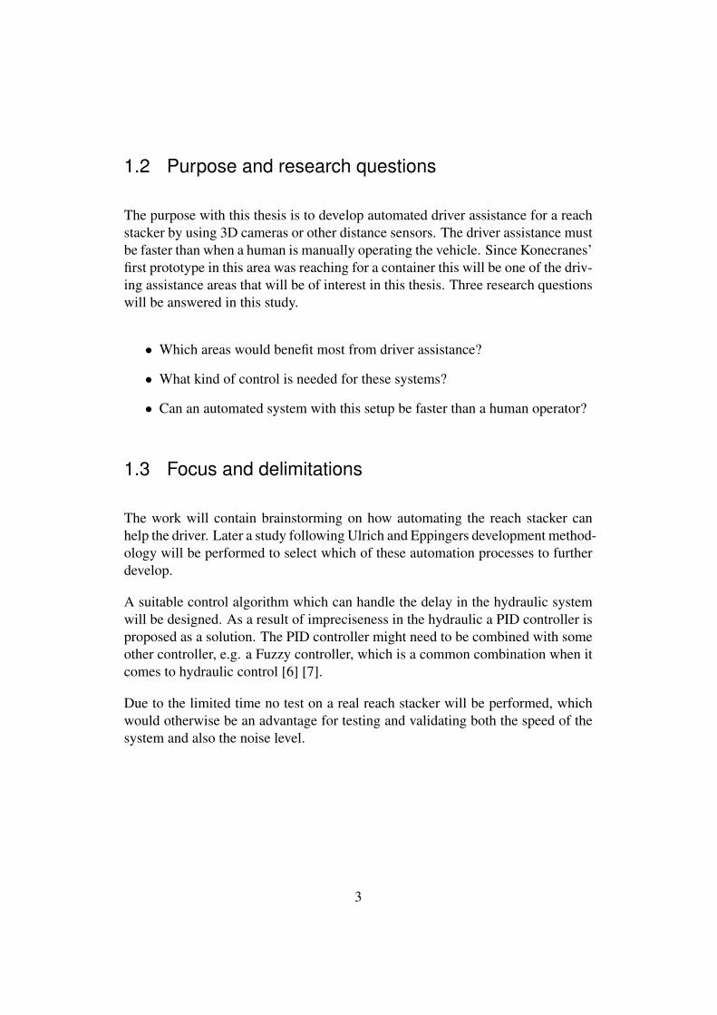
This prototype could, however, only move the lifting spreader in one direction oraround one axis at the time. Figure 1.1 illustrates the possible movements. Thespreader can move in X, Y and Z directions, it can rotate around the Z and Yaxis and finally it is possible to change the width of the spread. When the driverdoes this manually with the help of a joystick, can he move the spreader in alldirections at the same time. The movement of the lifting spreader is performedwith hydraulics, this means there is a delay in the movement.

1

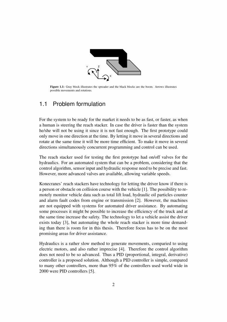
Figure 1.1: Gray block illustrates the spreader and the black blocks are the boom. Arrows illustratespossible movements and rotations.

1.1 Problem formulation

For the system to be ready for the market it needs to be as fast, or faster, as whena human is steering the reach stacker. In case the driver is faster than the systemhe/she will not be using it since it is not fast enough. The first prototype couldonly move in one direction at the time. By letting it move in several directions androtate at the same time it will be more time efficient. To make it move in severaldirections simultaneously concurrent programming and control can be used.

The reach stacker used for testing the first prototype had on/off valves for thehydraulics. For an automated system that can be a problem, considering that thecontrol algorithm, sensor input and hydraulic response need to be precise and fast.However, more advanced valves are available, allowing variable speeds.

Konecranes’ reach stackers have technology for letting the driver know if there isa person or obstacle on collision course with the vehicle [1]. The possibility to re-motely monitor vehicle data such as total lift load, hydraulic oil particles counterand alarm fault codes from engine or transmission [2]. However, the machinesare not equipped with systems for automated driver assistance. By automatingsome processes it might be possible to increase the efficiency of the truck and atthe same time increase the safety. The technology to let a vehicle assist the driverexists today [3], but automating the whole reach stacker is more time demand-ing than there is room for in this thesis. Therefore focus has to be on the mostpromising areas for driver assistance.

Hydraulics is a rather slow method to generate movements, comparied to usingelectric motors, and also rather imprecise [4]. Therefore the control algorithmdoes not need to be so advanced. Thus a PID (proportional, integral, derivative)controller is a proposed solution. Although a PID controller is simple, comparedto many other controllers, more than 95% of the controllers used world wide in2000 were PID controllers [5].

2

1.2 Purpose and research questions

The purpose with this thesis is to develop automated driver assistance for a reachstacker by using 3D cameras or other distance sensors. The driver assistance mustbe faster than when a human is manually operating the vehicle. Since Konecranes’first prototype in this area was reaching for a container this will be one of the driv-ing assistance areas that will be of interest in this thesis. Three research questionswill be answered in this study.

• Which areas would benefit most from driver assistance?

• What kind of control is needed for these systems?

• Can an automated system with this setup be faster than a human operator?

1.3 Focus and delimitations

The work will contain brainstorming on how automating the reach stacker canhelp the driver. Later a study following Ulrich and Eppingers development method-ology will be performed to select which of these automation processes to furtherdevelop.

A suitable control algorithm which can handle the delay in the hydraulic systemwill be designed. As a result of impreciseness in the hydraulic a PID controller isproposed as a solution. The PID controller might need to be combined with someother controller, e.g. a Fuzzy controller, which is a common combination when itcomes to hydraulic control [6] [7].

Due to the limited time no test on a real reach stacker will be performed, whichwould otherwise be an advantage for testing and validating both the speed of thesystem and also the noise level.

3

Chapter 2

Methodology

This chapter handles theories and tools applied in the report. Since this thesishandles several problems the following chapter are divided into three sections,Concept development, Automation of the spreader and Sensors.

2.1 Concept development

Since the timespan of this work was not big enough for developing a fully auto-mated reach stacker focus was directed to the most promising movements for au-tomation, here called Processes. To decide which of all processes to automate thework followed Karl T. Ulrich and Steven D. Eppingers methodology for ProductDevelopment [8]. By following their methodology the course of deciding whichprocesses to further work with becomes scientific and structured.

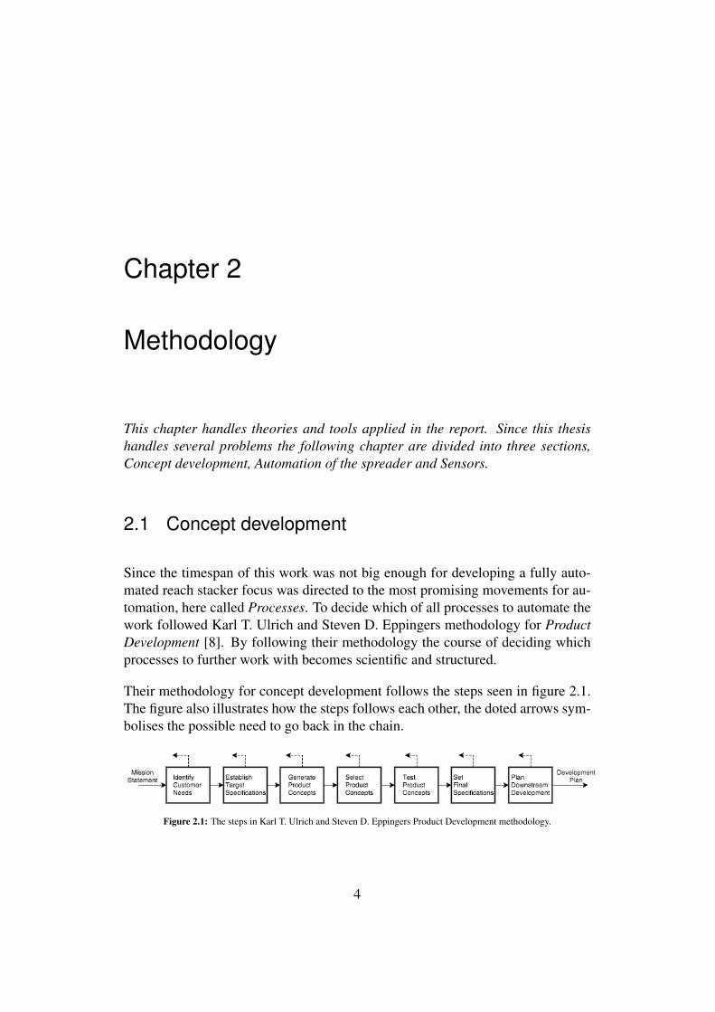
Their methodology for concept development follows the steps seen in figure 2.1.The figure also illustrates how the steps follows each other, the doted arrows sym-bolises the possible need to go back in the chain.

Figure 2.1: The steps in Karl T. Ulrich and Steven D. Eppingers Product Development methodology.

4

After the mission statement is established it is time for Identifying CustomerNeeds. The identification starts with gathering of raw data from the customers.This information was collected through interviews with customers, by watch-ing the the reach stacker in use and meetings with the technical department atKonecranes Lifttrucks AB. This raw data was then translated into customer needs,where it is important to define what the product should do and not how it shoulddo it. The needs are later organized in a hierarchical order, with primary andsecondary needs. With a hierarchical order completed the needs are then rankedagainst each other.

Next step is to Establish Target Specifications. Here a list of measurable units isgenerated which contains ideal and acceptable values. These values were com-posed through benchmarking and discussions with operators and the technicaldepartment.

After Establish Target Specifications is it time to Generate Product Concepts.Concepts are generated in several steps, the first is to clarify the problems, thensolutions to these are searched for both externally and internally. Searching ex-ternally in this case means to search for existing solutions for the problem andconsulting experts and users, while searching internally the knowledge and cre-ativity of the team is used while brainstorming for solutions. The last step in theconcept generation is to explore the combinations of all concepts systematically.This is carried out by categorizing the subsolutions.

Figure 2.1 shows that the next activity is Select Product Concepts. According tothe method this phase should be implemented in one or two steps, which are con-cept screening and concept scoring. In both these methods the concepts are ratedbut in the concept scoring the rating is also weighted depending on the impor-tance of the criteria. These criteria are selected based on the customer needs andthe needs from the company, e.g. low production cost. For both the screening andscoring a reference concept is used to rate the concepts to each other. Due to thecomplexity with comparing totally different concepts with each other neither thescreening nor scoring were used in this thesis. The selection was instead made asa discussion around the pros, cons and possibilities for the concepts.

Then the Test Product Concepts phase begins, which in this thesis was the testingcarried out in Matlab and Simulink, see section 2.2.

When the testing is completed is it possible to continue with Set Final Specifi-cations. These specifications are based on what values could be reached in thetesting phase.

5

The last step in the Karl T. Ulrich and Steven D. Eppingers product developmentmethodology [8] is Plan Downstream Development. The purpose of this activityis to facilitate the further development of the product. It contains a developmentschedule with time frames for further development and identification of resourcesneeded to finish the project.

All of the above mentioned steps, the steps in figure 2.1, involve three activitiesthat they all have in common. These are economic analysis, benchmarking ofcompetitive prototypes and build and test models and prototypes. The work ofthese three should be carried out along side the concept development. Reflectionover the result is also important at the end of every step.

2.2 Spreader automation

The process of developing a suitable algorithm for the container reaching startedwith a model built in Simulink [9], an add-on to Matlab [10]. Simulink is a graph-ical programming environment for modelling, simulating and analysing. Buildinga model in Simulink and then simulating the process, rather than testing with areal reach stacker, made it easier and faster to test and change parameters in thecontrol algorithm.

The model was built with the library Simscape [11], This library contains subli-braries. The skeleton of the model was constructed with the sublibrary SimMe-chanics, this contains the solid parts and joints that allow the arm and spreader tomove.

The real reach stacker uses hydraulics to move the spreader to the desired location.To imitate the behaviour of hydraulics Simscape has a library called SimHydraulic.This library makes it possible to simulate the whole hydraulic system with pumps,vents and moving parts. The hydraulic system is connected to the mechanical partsand enables movements of the arm and spreader.

For tuning of the actuator speeds the times in table 2.1 were the limit. The actuatorwas not allowed to be faster than times specified by Elme, appendix B.2, andKonecranes. These times are for when the actuator is under the maximum allowedstrain, when it is lifting a 45 ton container. In this table Spreader rotation isthe actuator which allows the spreader to rotate around the Z axis in figure 1.1.Spreader sideshift moves the spreader in Y direction and Spreader width makesthe spreader longer in the Y direction. Boom lift lifts or lowers the boom and

6

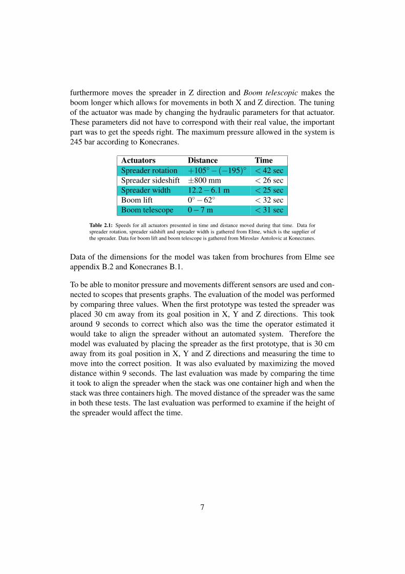
furthermore moves the spreader in Z direction and Boom telescopic makes theboom longer which allows for movements in both X and Z direction. The tuningof the actuator was made by changing the hydraulic parameters for that actuator.These parameters did not have to correspond with their real value, the importantpart was to get the speeds right. The maximum pressure allowed in the system is245 bar according to Konecranes.

Actuators Distance Time

Spreader rotation +105� � (�195)� < 42 secSpreader sideshift ±800 mm < 26 secSpreader width 12.2�6.1 m < 25 secBoom lift 0� �62� < 32 secBoom telescope 0�7 m < 31 sec

Table 2.1: Speeds for all actuators presented in time and distance moved during that time. Data forspreader rotation, spreader sidshift and spreader width is gathered from Elme, which is the supplier ofthe spreader. Data for boom lift and boom telescope is gathered from Miroslav Antolovic at Konecranes.

Data of the dimensions for the model was taken from brochures from Elme seeappendix B.2 and Konecranes B.1.

To be able to monitor pressure and movements different sensors are used and con-nected to scopes that presents graphs. The evaluation of the model was performedby comparing three values. When the first prototype was tested the spreader wasplaced 30 cm away from its goal position in X, Y and Z directions. This tookaround 9 seconds to correct which also was the time the operator estimated itwould take to align the spreader without an automated system. Therefore themodel was evaluated by placing the spreader as the first prototype, that is 30 cmaway from its goal position in X, Y and Z directions and measuring the time tomove into the correct position. It was also evaluated by maximizing the moveddistance within 9 seconds. The last evaluation was made by comparing the timeit took to align the spreader when the stack was one container high and when thestack was three containers high. The moved distance of the spreader was the samein both these tests. The last evaluation was performed to examine if the height ofthe spreader would affect the time.

7

2.2.1 Control

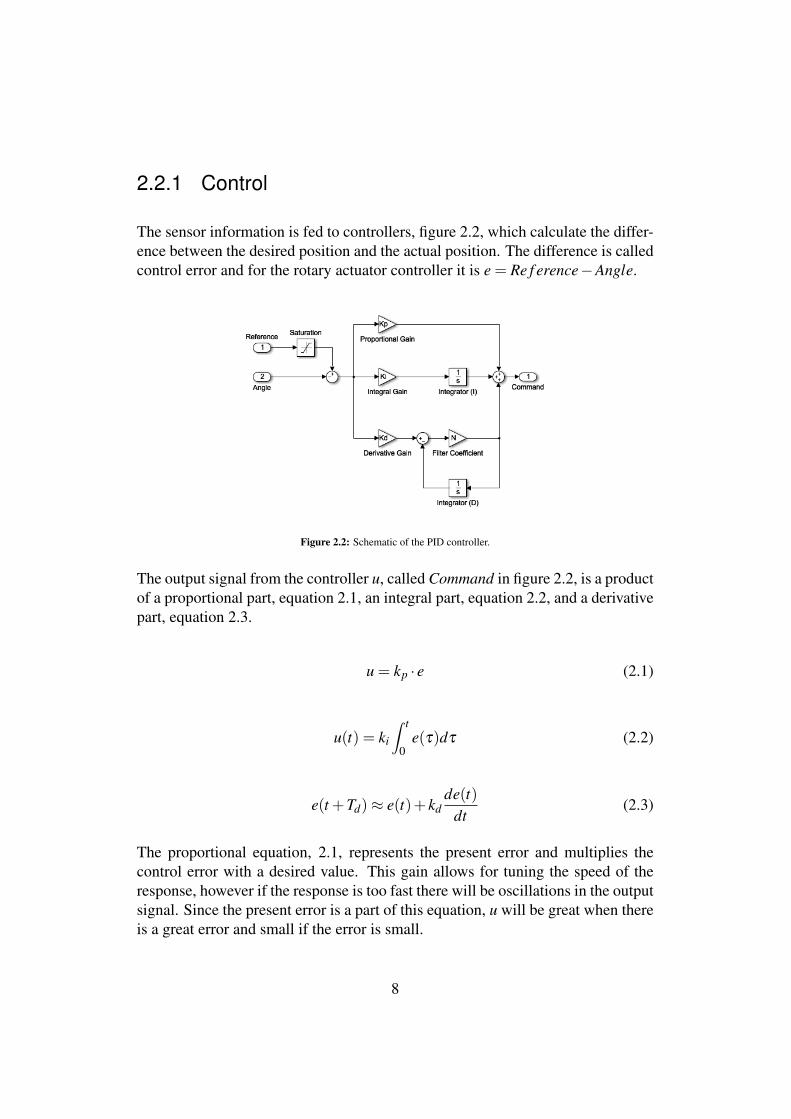
The sensor information is fed to controllers, figure 2.2, which calculate the differ-ence between the desired position and the actual position. The difference is calledcontrol error and for the rotary actuator controller it is e = Re f erence�Angle.

Figure 2.2: Schematic of the PID controller.

The output signal from the controller u, called Command in figure 2.2, is a productof a proportional part, equation 2.1, an integral part, equation 2.2, and a derivativepart, equation 2.3.

u = kp · e (2.1)

u(t) = ki

Z t

0e(t)dt (2.2)

e(t +Td)⇡ e(t)+ kdde(t)

dt(2.3)

The proportional equation, 2.1, represents the present error and multiplies thecontrol error with a desired value. This gain allows for tuning the speed of theresponse, however if the response is too fast there will be oscillations in the outputsignal. Since the present error is a part of this equation, u will be great when thereis a great error and small if the error is small.

8

The future, e, Td units head is predicted with the derivative equation, 2.3.

By combining these three equation, retrieved from Karl Johan Astrom and RichardM. Murray book Feedback Systems [12], the control algorithm observes the past,the present and the future. The final control equation then becomes 2.4 which inSimulink looks like figure 2.2.

u(t) = kpe(t)+ ki

Z t

0e(t)dt + kd

de(t)dt

(2.4)

2.3 Sensors

The controllers need reference values for the desired location they are moving to-wards. Since the reach stacker is working with external objects these referencevalues can not be hard coded, they must be fetched from the surrounding. Inputsto computerised systems from the real world can come from sensors of differ-ent sorts. Therefore an evaluation on sensors was performed. Also this processfollowed Ulrich and Eppingers methodology for product development.

Since this thesis is a feasibility study the sensors were not tested. The resultpresented further on in this report is only recommendations worth thinking ofwhen building a prototype. The recommendations are based on information aboutthe sensors.

The sensors send values to a State Machine, which is built with a Simulink librarycalled Stateflow [13]. The state machine is acting based on where the spreader is inrelation to its goal position. It calculates new reference values for the controllersto act on.

9

Chapter 3

Results

This chapter contains the results of the Concept development, section 3.1, and theinformation that led to the result. Section 3.2, about the Simulink model, containsa subsection about the Mechanical and Hydraulic model, section 3.2.1, and asubsection for the Control, 3.2.2. The results about the Sensors are presented insection 3.3 which contains both sensor technologies and placement.

3.1 Concept development

3.1.1 Customer statements

To better know the customer needs a meeting was held at one of Konecranes cus-tomer.

During the meeting four questions were discussed. These were:

• What part in the reach stackers driving cycle can be improved by automa-tion?

• What must be thought of if a process is automated?

• Situations where automation should not be used?

• How can the operator steer the process and what information does he/sheneed?

10

The summary of this meeting can be found in appendix A.1.

3.1.2 Customer needs

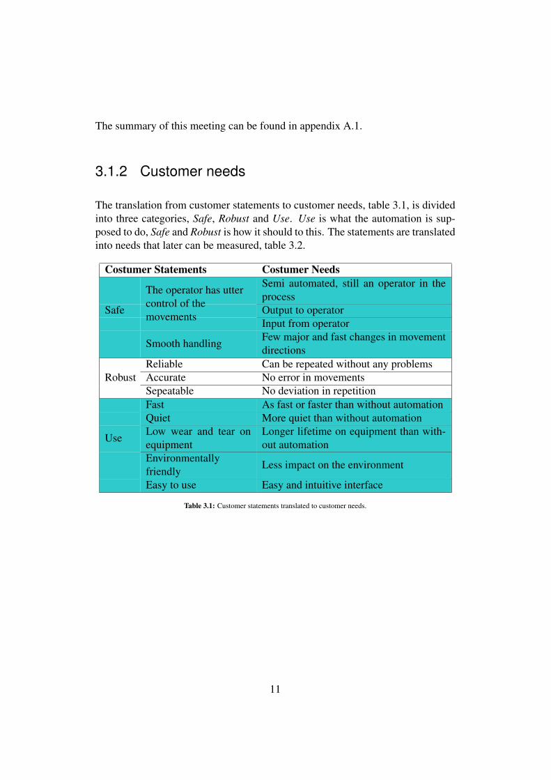
The translation from customer statements to customer needs, table 3.1, is dividedinto three categories, Safe, Robust and Use. Use is what the automation is sup-posed to do, Safe and Robust is how it should to this. The statements are translatedinto needs that later can be measured, table 3.2.

Costumer Statements Costumer Needs

Semi automated, still an operator in theprocessOutput to operator

The operator has uttercontrol of themovements Input from operator

Safe

Smooth handling Few major and fast changes in movementdirections

RobustReliable Can be repeated without any problemsAccurate No error in movementsSepeatable No deviation in repetitionFast As fast or faster than without automationQuiet More quiet than without automationLow wear and tear onequipment

Longer lifetime on equipment than with-out automation

Environmentallyfriendly Less impact on the environment

Use

Easy to use Easy and intuitive interface

Table 3.1: Customer statements translated to customer needs.

11

There are two reason to let the operator have the utter control of the movements.The first is that making the system fully automated means a higher degree ofsafety must be reached, described in appendix A.1. The second also has to dowith safety, allowing the vehicle to move fully automated may have devastatingconsequences. For example, if the reach stacker is operating with a levitated con-tainer and the automated system stops the vehicle due to a nearby object it mayresult in a vehicle rollover. Smooth handling is due to the same reason, with aheavy container levitated can fast movements in a new direction results in greatforces which ought to be avoided.

The system is supposed to deliver on the same level every time, it should be Ro-bust. This category consists of statements that it should be reliable, accurate andable to repeat the same movement several times.

The Use category is what will be the improvements with the new system. It shouldbe faster, make less noise, be kinder to the equipment and finally be easy for theoperator to use.

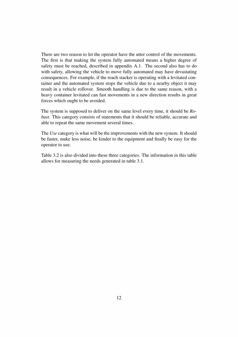
Table 3.2 is also divided into these three categories. The information in this tableallows for measuring the needs generated in table 3.1.

12

Costumer Needs Measurable Units Unit

Semi automated, still an operatorin the process

Binary

Output to operator BinaryInput from operator BinaryFew major and fast changes inmovement directions

Times of changes in movementdirections greater than rad/sec

Times

Can be repeated without anyproblems

Number of repeated cycles Times

No error in movements Deviation from target mmNo deviation in repetition Deviation from last cycle mmAs fast or faster than without au-tomation

Percentage of seconds fasterthan a human operator

%

As quiet or more quiet than with-out automation

Percentage of decibel lower thana human operator

%

As long or longer lifetime onequipment than without automa-tion

Percentage of hours longer life-time than a human operator

%

Less impact on the environment Precentage of liters of petrolused for a drive cycle

%

Easy and intuitive interface Binary

Table 3.2: Customer needs translated to measurable units.

Binary here means yes or no, either the need is met or not. The other units gener-ated is for distance [mm], how many times a specific event occurs and percentageof a new value compared to a value without automation.

3.1.3 Target specifications

A final product should contain all the costumer needs with a binary unit. Thecostumer needs within the robust category is affected by the sensors which arepresented in section 3.3. The target specification regarding speed is that a move-ment of 0.3m in all three directions (X, Y and Z) should take less than 9 seconds.The accuracy of the spreader alignment must be within 5 cm to allow for a lockbetween the spreader and the container. Comparing the sound, the lifetime andthe impact on the environment is not within the span of this thesis.

13

3.1.4 Generate concepts

After discussing possibilities, studying of reach stackers in action and benchmark-ing a few concepts were generated.

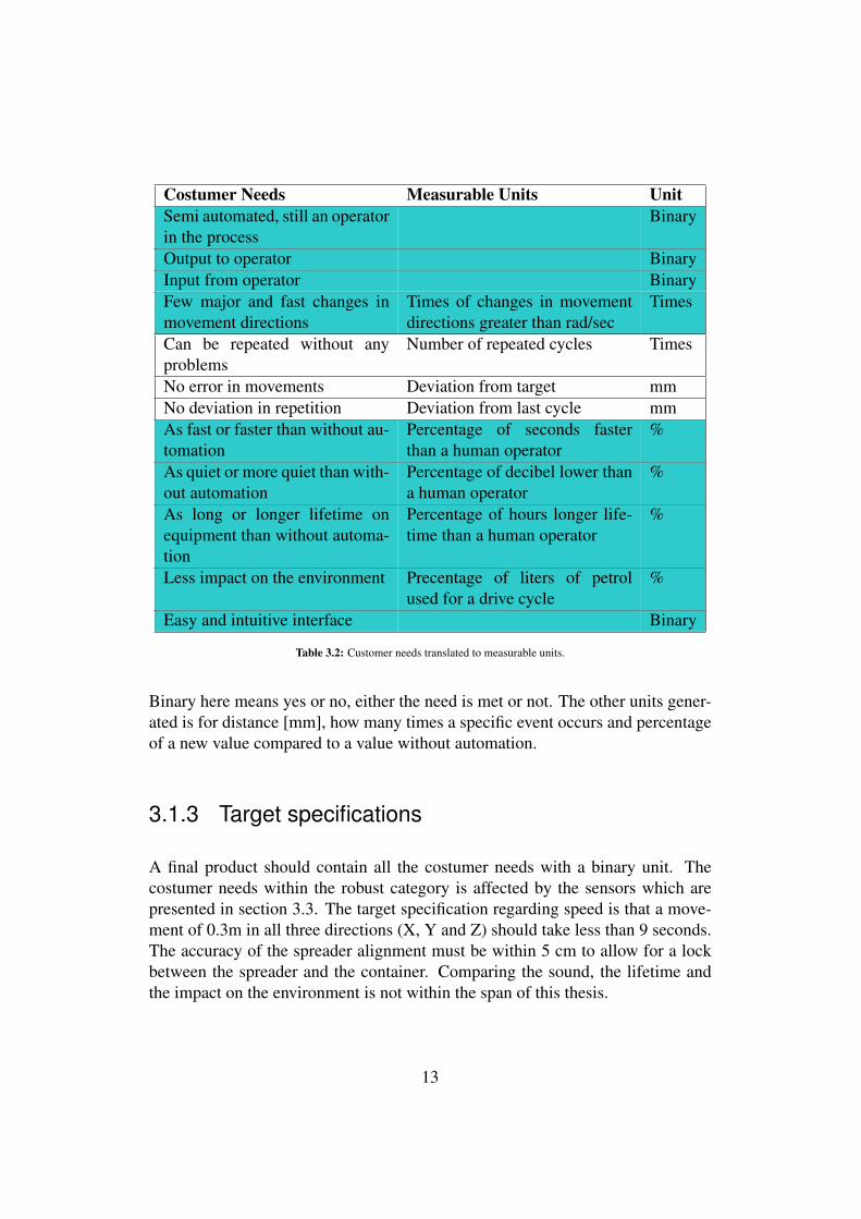
• Concept Pick Up: Automatic spreader alignment when reaching for a con-tainer, figure 3.1a.

• Concept Drop down: Automatic spreader alignment when releasing a con-tainer, figure 3.1b.

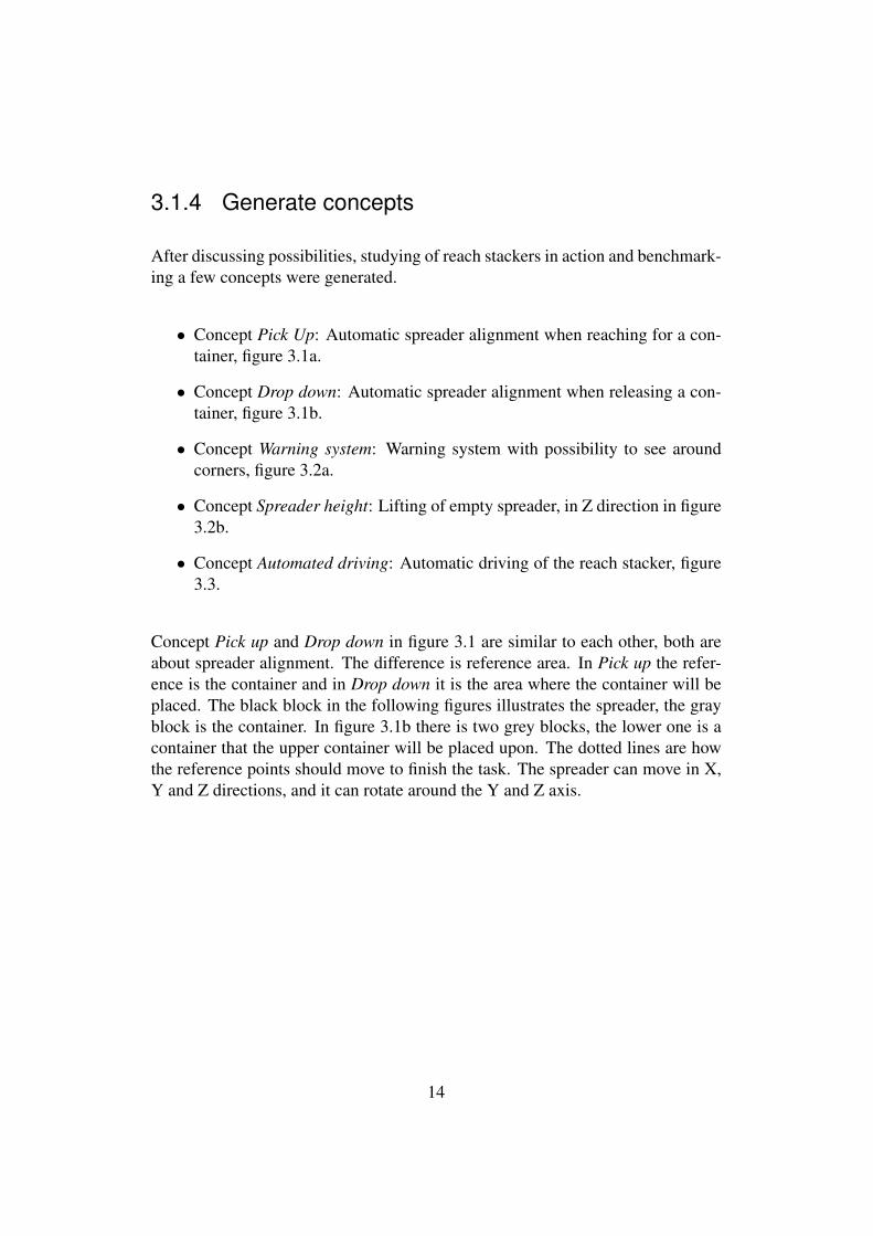
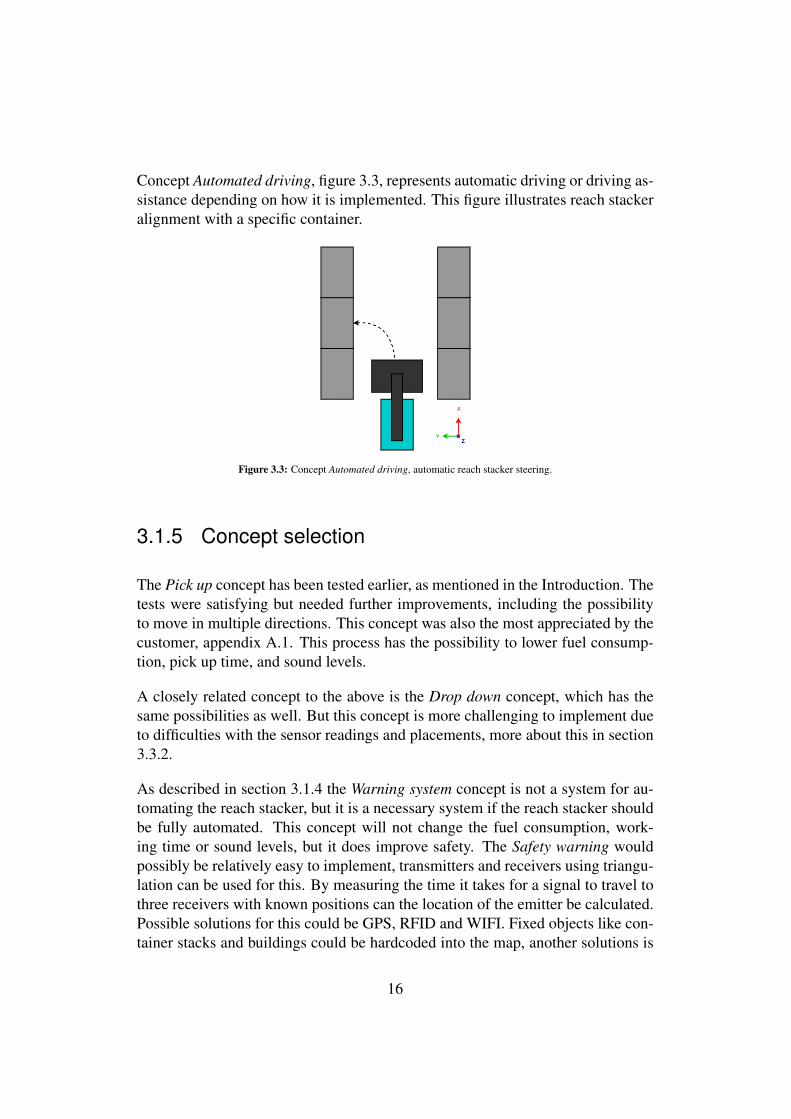
• Concept Warning system: Warning system with possibility to see aroundcorners, figure 3.2a.

• Concept Spreader height: Lifting of empty spreader, in Z direction in figure3.2b.

• Concept Automated driving: Automatic driving of the reach stacker, figure3.3.

Concept Pick up and Drop down in figure 3.1 are similar to each other, both areabout spreader alignment. The difference is reference area. In Pick up the refer-ence is the container and in Drop down it is the area where the container will beplaced. The black block in the following figures illustrates the spreader, the grayblock is the container. In figure 3.1b there is two grey blocks, the lower one is acontainer that the upper container will be placed upon. The dotted lines are howthe reference points should move to finish the task. The spreader can move in X,Y and Z directions, and it can rotate around the Y and Z axis.

14

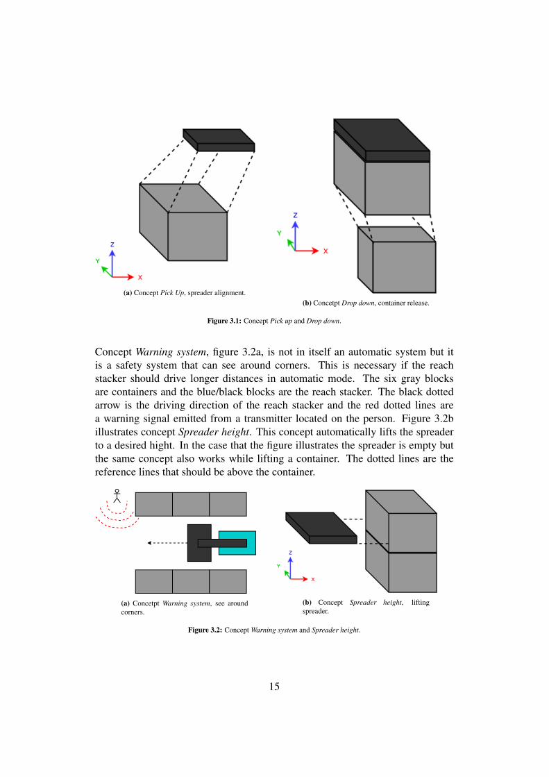
(a) Concept Pick Up, spreader alignment.(b) Concetpt Drop down, container release.

Figure 3.1: Concept Pick up and Drop down.

Concept Warning system, figure 3.2a, is not in itself an automatic system but itis a safety system that can see around corners. This is necessary if the reachstacker should drive longer distances in automatic mode. The six gray blocksare containers and the blue/black blocks are the reach stacker. The black dottedarrow is the driving direction of the reach stacker and the red dotted lines area warning signal emitted from a transmitter located on the person. Figure 3.2billustrates concept Spreader height. This concept automatically lifts the spreaderto a desired hight. In the case that the figure illustrates the spreader is empty butthe same concept also works while lifting a container. The dotted lines are thereference lines that should be above the container.

(a) Concetpt Warning system, see aroundcorners.

(b) Concept Spreader height, liftingspreader.

Figure 3.2: Concept Warning system and Spreader height.

15

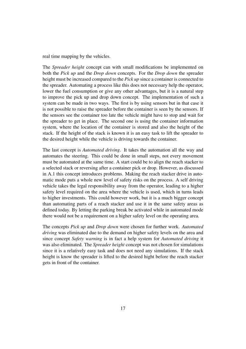
Concept Automated driving, figure 3.3, represents automatic driving or driving as-sistance depending on how it is implemented. This figure illustrates reach stackeralignment with a specific container.

Figure 3.3: Concept Automated driving, automatic reach stacker steering.

3.1.5 Concept selection

The Pick up concept has been tested earlier, as mentioned in the Introduction. Thetests were satisfying but needed further improvements, including the possibilityto move in multiple directions. This concept was also the most appreciated by thecustomer, appendix A.1. This process has the possibility to lower fuel consump-tion, pick up time, and sound levels.

A closely related concept to the above is the Drop down concept, which has thesame possibilities as well. But this concept is more challenging to implement dueto difficulties with the sensor readings and placements, more about this in section3.3.2.

As described in section 3.1.4 the Warning system concept is not a system for au-tomating the reach stacker, but it is a necessary system if the reach stacker shouldbe fully automated. This concept will not change the fuel consumption, work-ing time or sound levels, but it does improve safety. The Safety warning wouldpossibly be relatively easy to implement, transmitters and receivers using triangu-lation can be used for this. By measuring the time it takes for a signal to travel tothree receivers with known positions can the location of the emitter be calculated.Possible solutions for this could be GPS, RFID and WIFI. Fixed objects like con-tainer stacks and buildings could be hardcoded into the map, another solutions is

16

real time mapping by the vehicles.

The Spreader height concept can with small modifications be implemented onboth the Pick up and the Drop down concepts. For the Drop down the spreaderheight must be increased compared to the Pick up since a container is connected tothe spreader. Automating a process like this does not necessary help the operator,lower the fuel consumption or give any other advantages, but it is a natural stepto improve the pick up and drop down concept. The implementation of such asystem can be made in two ways. The first is by using sensors but in that case itis not possible to raise the spreader before the container is seen by the sensors. Ifthe sensors see the container too late the vehicle might have to stop and wait forthe spreader to get in place. The second one is using the container informationsystem, where the location of the container is stored and also the height of thestack. If the height of the stack is known it is an easy task to lift the spreader tothe desired height while the vehicle is driving towards the container.

The last concept is Automated driving. It takes the automation all the way andautomates the steering. This could be done in small steps, not every movementmust be automated at the same time. A start could be to align the reach stacker toa selected stack or reversing after a container pick or drop. However, as discussedin A.1 this concept introduces problems. Making the reach stacker drive in auto-matic mode puts a whole new level of safety risks on the process. A self drivingvehicle takes the legal responsibility away from the operator, leading to a highersafety level required on the area where the vehicle is used, which in turns leadsto higher investments. This could however work, but it is a much bigger conceptthan automating parts of a reach stacker and use it in the same safety areas asdefined today. By letting the parking break be activated while in automated modethere would not be a requirement on a higher safety level on the operating area.

The concepts Pick up and Drop down were chosen for further work. Automateddriving was eliminated due to the demand on higher safety levels on the area andsince concept Safety warning is in fact a help system for Automated driving itwas also eliminated. The Spreader height concept was not chosen for simulationssince it is a relatively easy task and does not need any simulations. If the stackheight is know the spreader is lifted to the desired hight before the reach stackergets in front of the container.

17

3.2 Simulink model

3.2.1 Mechanical and hydraulic model

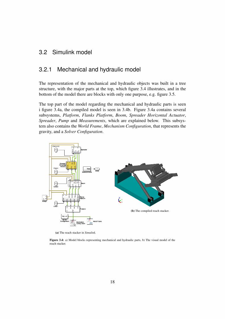
The representation of the mechanical and hydraulic objects was built in a treestructure, with the major parts at the top, which figure 3.4 illustrates, and in thebottom of the model there are blocks with only one purpose, e.g. figure 3.5.

The top part of the model regarding the mechanical and hydraulic parts is seeni figure 3.4a, the compiled model is seen in 3.4b. Figure 3.4a contains severalsubsystems, Platform, Flanks Platform, Boom, Spreader Horizontal Actuator,Spreader, Pump and Measurements, which are explained below. This subsys-tem also contains the World Frame, Mechanism Configuration, that represents thegravity, and a Solver Configuration.

(a) The reach stacker in Simulink.

(b) The compiled reach stacker.

Figure 3.4: a) Model blocks representing mechanical and hydraulic parts, b) The visual model of thereach stacker.

18

The input to this subsystem is the Command signal Cmd, seen in figure 3.4a. Thissignal is the output from the controller. It is a vector of six signals that is sentforward into four subsystems. Deeper into the model the correct signal for thatspecific actuator is collected, in figure 3.11 this signal collection is made in theS-SP block.

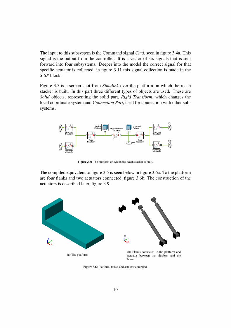
Figure 3.5 is a screen shot from Simulink over the platform on which the reachstacker is built. In this part three different types of objects are used. These areSolid objects, representing the solid part, Rigid Transform, which changes thelocal coordinate system and Connection Port, used for connection with other sub-systems.

Figure 3.5: The platform on which the reach stacker is built.

The compiled equivalent to figure 3.5 is seen below in figure 3.6a. To the platformare four flanks and two actuators connected, figure 3.6b. The construction of theactuators is described later, figure 3.9.

(a) The platform.(b) Flanks connected to the platform andactuator between the platform and theboom.

Figure 3.6: Platform, flanks and actuator compiled.

19

The compiled subsystems to Boom and Spreader in figure 3.4a is illustrated infigure 3.7.

(a) The boom.(b) The spreader.

Figure 3.7: The boom and the spreader compiled.

Both figures 3.7a and 3.7b are built with more subsystems inside them. For exam-ple the spreader has three kinds of actuators built inside it, one for changing thewidth of the spreader, one for rotating it and one for moving it longitudinal.

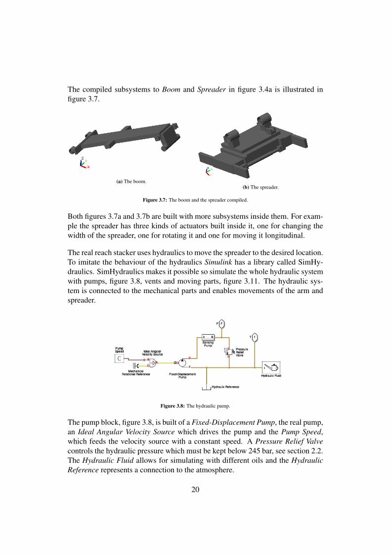
The real reach stacker uses hydraulics to move the spreader to the desired location.To imitate the behaviour of the hydraulics Simulink has a library called SimHy-draulics. SimHydraulics makes it possible so simulate the whole hydraulic systemwith pumps, figure 3.8, vents and moving parts, figure 3.11. The hydraulic sys-tem is connected to the mechanical parts and enables movements of the arm andspreader.

Figure 3.8: The hydraulic pump.

The pump block, figure 3.8, is built of a Fixed-Displacement Pump, the real pump,an Ideal Angular Velocity Source which drives the pump and the Pump Speed,which feeds the velocity source with a constant speed. A Pressure Relief Valvecontrols the hydraulic pressure which must be kept below 245 bar, see section 2.2.The Hydraulic Fluid allows for simulating with different oils and the HydraulicReference represents a connection to the atmosphere.

20

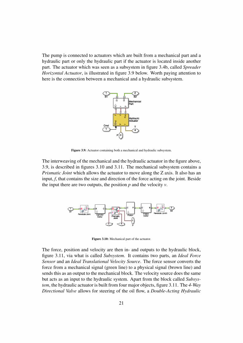
The pump is connected to actuators which are built from a mechanical part and ahydraulic part or only the hydraulic part if the actuator is located inside anotherpart. The actuator which was seen as a subsystem in figure 3.4b, called SpreaderHorizontal Actuator, is illustrated in figure 3.9 below. Worth paying attention tohere is the connection between a mechanical and a hydraulic subsystem.

Figure 3.9: Actuator containing both a mechanical and hydraulic subsystem.

The interweaving of the mechanical and the hydraulic actuator in the figure above,3.9, is described in figures 3.10 and 3.11. The mechanical subsystem contains aPrismatic Joint which allows the actuator to move along the Z axis. It also has aninput, f, that contains the size and direction of the force acting on the joint. Besidethe input there are two outputs, the position p and the velocity v.

Figure 3.10: Mechanical part of the actuator.

The force, position and velocity are then in- and outputs to the hydraulic block,figure 3.11, via what is called Subsystem. It contains two parts, an Ideal ForceSensor and an Ideal Translational Velocity Source. The force sensor converts theforce from a mechanical signal (green line) to a physical signal (brown line) andsends this as an output to the mechanical block. The velocity source does the samebut acts as an input to the hydraulic system. Apart from the block called Subsys-tem, the hydraulic actuator is built from four major objects, figure 3.11. The 4-WayDirectional Valve allows for steering of the oil flow, a Double-Acting Hydraulic

21

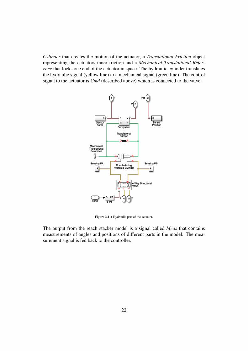
Cylinder that creates the motion of the actuator, a Translational Friction objectrepresenting the actuators inner friction and a Mechanical Translational Refer-ence that locks one end of the actuator in space. The hydraulic cylinder translatesthe hydraulic signal (yellow line) to a mechanical signal (green line). The controlsignal to the actuator is Cmd (described above) which is connected to the valve.

Figure 3.11: Hydraulic part of the actuator.

The output from the reach stacker model is a signal called Meas that containsmeasurements of angles and positions of different parts in the model. The mea-surement signal is fed back to the controller.

22

3.2.2 Control

Figures 3.12b to 3.15 illustrate the measured signal (blue line) and the referencesignal (red line). Degrees of rotation can be seen on the Y axis and the X axisrepresents the time.

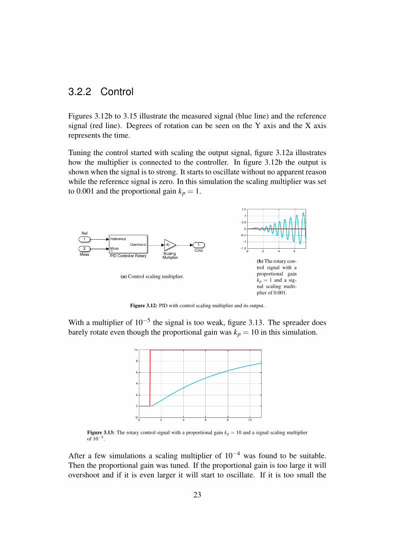
Tuning the control started with scaling the output signal, figure 3.12a illustrateshow the multiplier is connected to the controller. In figure 3.12b the output isshown when the signal is to strong. It starts to oscillate without no apparent reasonwhile the reference signal is zero. In this simulation the scaling multiplier was setto 0.001 and the proportional gain kp = 1.

(a) Control scaling multiplier.

(b) The rotary con-trol signal with aproportional gainkp = 1 and a sig-nal scaling multi-plier of 0.001.

Figure 3.12: PID with control scaling multiplier and its output.

With a multiplier of 10�5 the signal is too weak, figure 3.13. The spreader doesbarely rotate even though the proportional gain was kp = 10 in this simulation.

Figure 3.13: The rotary control signal with a proportional gain kp = 10 and a signal scaling multiplierof 10�5.

After a few simulations a scaling multiplier of 10�4 was found to be suitable.Then the proportional gain was tuned. If the proportional gain is too large it willovershoot and if it is even larger it will start to oscillate. If it is too small the

23

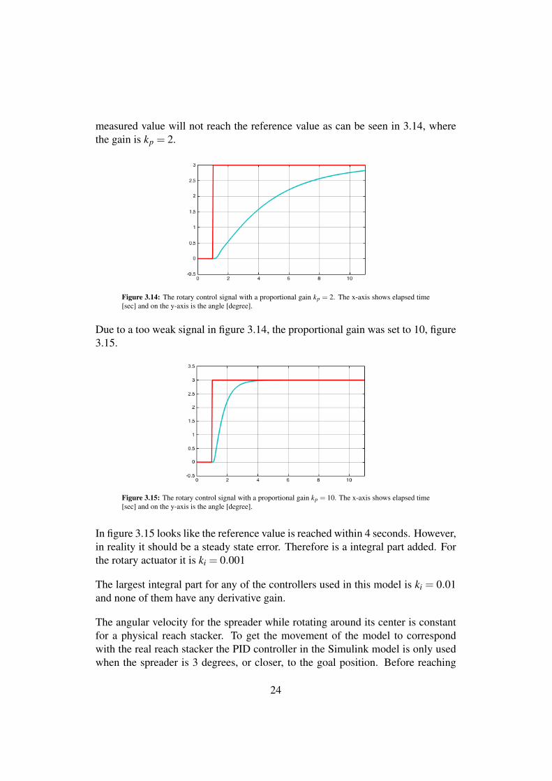
measured value will not reach the reference value as can be seen in 3.14, wherethe gain is kp = 2.

Figure 3.14: The rotary control signal with a proportional gain kp = 2. The x-axis shows elapsed time[sec] and on the y-axis is the angle [degree].

Due to a too weak signal in figure 3.14, the proportional gain was set to 10, figure3.15.

Figure 3.15: The rotary control signal with a proportional gain kp = 10. The x-axis shows elapsed time[sec] and on the y-axis is the angle [degree].

In figure 3.15 looks like the reference value is reached within 4 seconds. However,in reality it should be a steady state error. Therefore is a integral part added. Forthe rotary actuator it is ki = 0.001

The largest integral part for any of the controllers used in this model is ki = 0.01and none of them have any derivative gain.

The angular velocity for the spreader while rotating around its center is constantfor a physical reach stacker. To get the movement of the model to correspondwith the real reach stacker the PID controller in the Simulink model is only usedwhen the spreader is 3 degrees, or closer, to the goal position. Before reaching

24

the 3 degree limit, the spreader is set to reach 1000/-1000 degrees, depending ondirection. This allows for a constant speed even when the spreader gets closer toits end position. However this controller is not suitable when the the initial erroris just a few degrees.

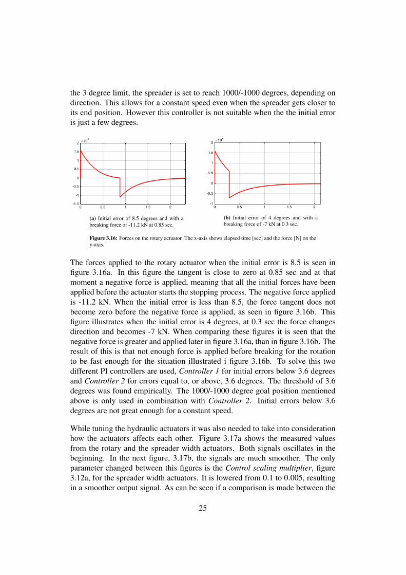
(a) Initial error of 8.5 degrees and with abreaking force of -11.2 kN at 0.85 sec.

(b) Initial error of 4 degrees and with abreaking force of -7 kN at 0.3 sec.

Figure 3.16: Forces on the rotary actuator. The x-axis shows elapsed time [sec] and the force [N] on they-axis.

The forces applied to the rotary actuator when the initial error is 8.5 is seen infigure 3.16a. In this figure the tangent is close to zero at 0.85 sec and at thatmoment a negative force is applied, meaning that all the initial forces have beenapplied before the actuator starts the stopping process. The negative force appliedis -11.2 kN. When the initial error is less than 8.5, the force tangent does notbecome zero before the negative force is applied, as seen in figure 3.16b. Thisfigure illustrates when the initial error is 4 degrees, at 0.3 sec the force changesdirection and becomes -7 kN. When comparing these figures it is seen that thenegative force is greater and applied later in figure 3.16a, than in figure 3.16b. Theresult of this is that not enough force is applied before breaking for the rotationto be fast enough for the situation illustrated i figure 3.16b. To solve this twodifferent PI controllers are used, Controller 1 for initial errors below 3.6 degreesand Controller 2 for errors equal to, or above, 3.6 degrees. The threshold of 3.6degrees was found empirically. The 1000/-1000 degree goal position mentionedabove is only used in combination with Controller 2. Initial errors below 3.6degrees are not great enough for a constant speed.

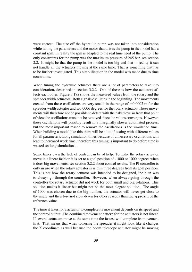
While tuning the hydraulic actuators it was also needed to take into considerationhow the actuators affects each other. Figure 3.17a shows the measured valuesfrom the rotary and the spreader width actuators. Both signals oscillates in thebeginning. In the next figure, 3.17b, the signals are much smoother. The onlyparameter changed between this figures is the Control scaling multiplier, figure3.12a, for the spreader width actuators. It is lowered from 0.1 to 0.005, resultingin a smoother output signal. As can be seen if a comparison is made between the

25

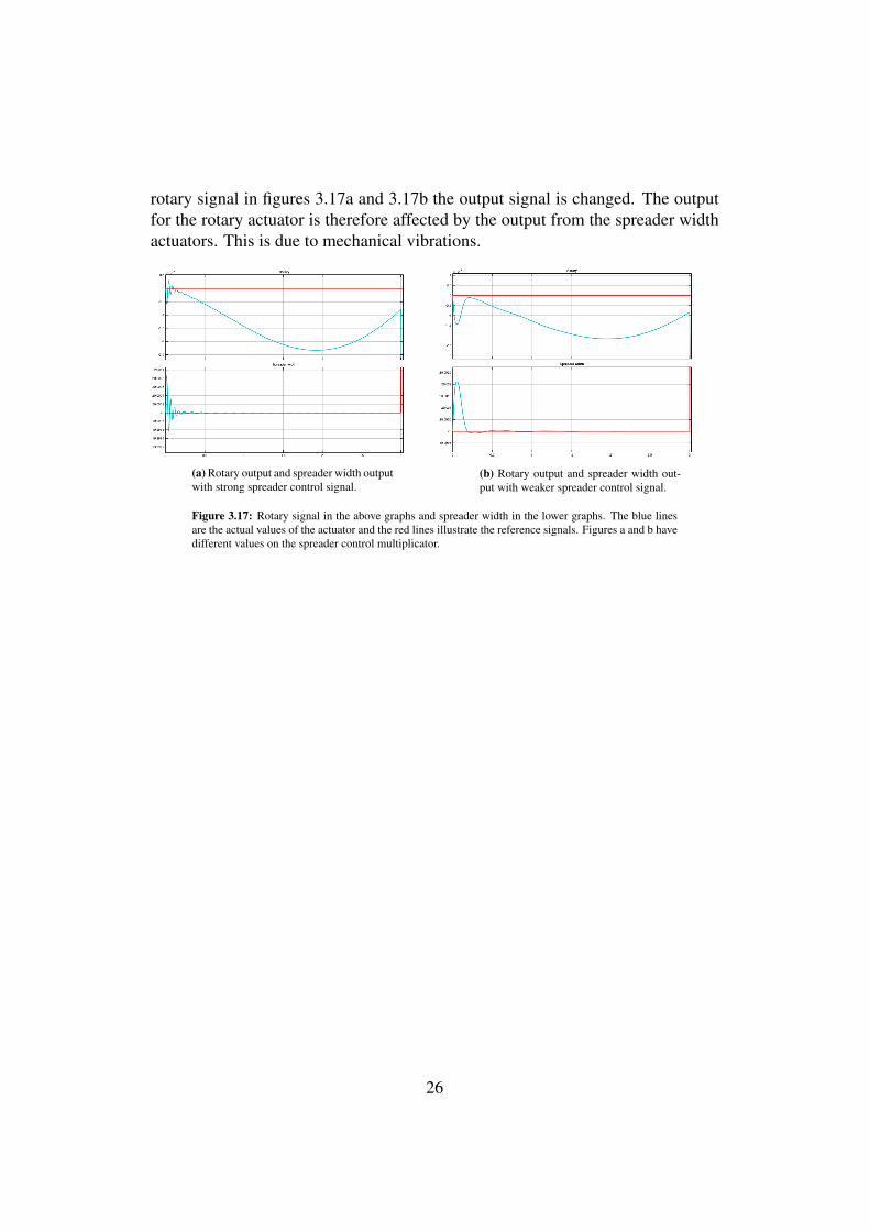
rotary signal in figures 3.17a and 3.17b the output signal is changed. The outputfor the rotary actuator is therefore affected by the output from the spreader widthactuators. This is due to mechanical vibrations.

(a) Rotary output and spreader width outputwith strong spreader control signal.

(b) Rotary output and spreader width out-put with weaker spreader control signal.

Figure 3.17: Rotary signal in the above graphs and spreader width in the lower graphs. The blue linesare the actual values of the actuator and the red lines illustrate the reference signals. Figures a and b havedifferent values on the spreader control multiplicator.

26

3.2.3 Movement calculations

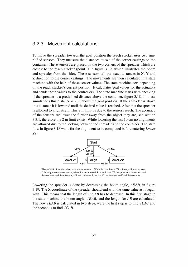
To move the spreader towards the goal position the reach stacker uses two sim-plified sensors. They measure the distances to two of the corner castings on thecontainer. These sensors are placed on the two corners of the spreader which areclosest to the reach stacker (point D in figure 3.19, which illustrates the boomand spreader from the side). These sensors tell the exact distances in X, Y andZ direction to the corner castings. The movements are then calculated in a statemachine with the help of these sensor values. The state machine acts dependingon the reach stacker’s current position. It calculates goal values for the actuatorsand sends these values to the controllers. The state machine starts with checkingif the spreader is a predefined distance above the container, figure 3.18. In thesesimulations this distance is 2 m above the goal position. If the spreader is abovethis distance it is lowered until the desired value is reached. After that the spreaderis allowed to align itself. This 2 m limit is due to the sensors reach. The accuracyof the sensors are lower the further away from the object they are, see section3.3.1, therefore the 2 m limit exists. While lowering the last 10 cm no alignmentsare allowed due to the locking between the spreader and the container. The stateflow in figure 3.18 waits for the alignment to be completed before entering LowerZ2.

Figure 3.18: State flow chart over the movements. While in state Lower Z1 is it only allowed to lowerZ. In Align movements in every direction are allowed. In state Lower Z2 the spreader is connected withthe container and therefore only allowed to lower Z the last 10 cm between itself and the container.

Lowering the spreader is done by decreasing the boom angle, 6 EAB, in figure3.19. The X coordinate of the spreader should end with the same value as it beganwith. This means that the length of line AB has to decrease. In this first stage inthe state machine the boom angle, 6 EAB, and the length for AB are calculated.The new 6 EAB is calculated in two steps, were the first step is to find 6 EAC andthe second is to find 6 CAB.

27

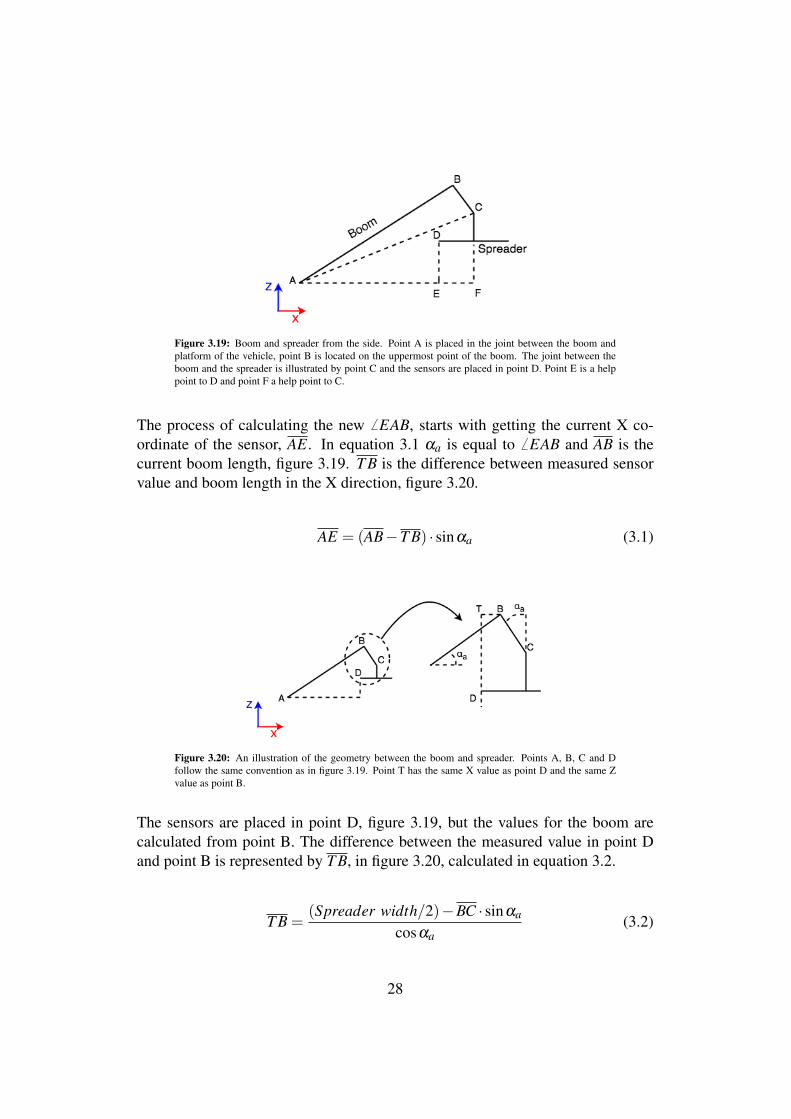
Figure 3.19: Boom and spreader from the side. Point A is placed in the joint between the boom andplatform of the vehicle, point B is located on the uppermost point of the boom. The joint between theboom and the spreader is illustrated by point C and the sensors are placed in point D. Point E is a helppoint to D and point F a help point to C.

The process of calculating the new 6 EAB, starts with getting the current X co-ordinate of the sensor, AE. In equation 3.1 aa is equal to 6 EAB and AB is thecurrent boom length, figure 3.19. T B is the difference between measured sensorvalue and boom length in the X direction, figure 3.20.

AE = (AB�T B) · sinaa (3.1)

Figure 3.20: An illustration of the geometry between the boom and spreader. Points A, B, C and Dfollow the same convention as in figure 3.19. Point T has the same X value as point D and the same Zvalue as point B.

The sensors are placed in point D, figure 3.19, but the values for the boom arecalculated from point B. The difference between the measured value in point Dand point B is represented by T B, in figure 3.20, calculated in equation 3.2.

T B =(Spreader width/2)�BC · sinaa

cosaa(3.2)

28

With AE known, it is easy to get AF , equation 3.3. In equation 3.4 the oppositeside to 6 EAC is calculated. Spreader height is the total height of the spreader, thatis the Z value between point C and D, CDZ .

AF = AE +Spreader width

2(3.3) CF = DE +Spreader height (3.4)

By using the Pythagorean theorem, it is now possible to calculate AC, equation3.5. By using the Pythagorean theorem again AB is found in equation 3.6 whereBC is the fixed length on the boom.

AC =

qAF2

+CF2 (3.5) AB =

qAC2 �BC2 (3.6)

With all sides known it is possible to calculate the angels 6 EAC, ab, in equa-tion 3.7, and 6 CAB, ac, in equation 3.8. From these two 6 EAB is calculated inequation 3.9, where aa is 6 EAB.

ab = arctanCFAF

(3.7)ac = arcsin

BCAC

(3.8)

aa = ab +ac (3.9)

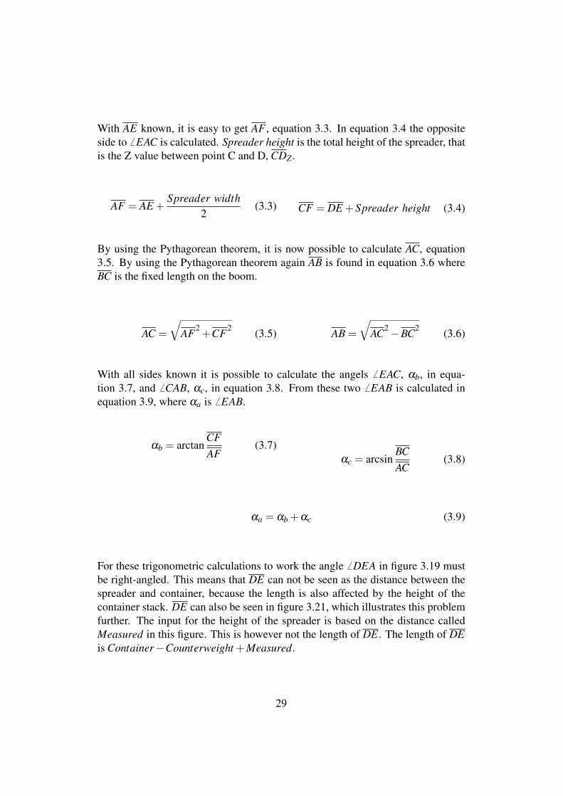
For these trigonometric calculations to work the angle 6 DEA in figure 3.19 mustbe right-angled. This means that DE can not be seen as the distance between thespreader and container, because the length is also affected by the height of thecontainer stack. DE can also be seen in figure 3.21, which illustrates this problemfurther. The input for the height of the spreader is based on the distance calledMeasured in this figure. This is however not the length of DE. The length of DEis Container�Counterweight +Measured.

29

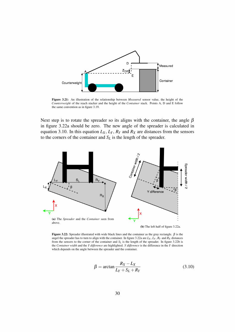
Figure 3.21: An illustration of the relationship between Measured sensor value, the height of theCounterweight of the reach stacker and the height of the Container stack. Points A, D and E followthe same convention as in figure 3.19.

Next step is to rotate the spreader so its aligns with the container, the angle bin figure 3.22a should be zero. The new angle of the spreader is calculated inequation 3.10. In this equation LX , LY , RY and RX are distances from the sensorsto the corners of the container and SL is the length of the spreader.

(a) The Spreader and the Container seen fromabove.

(b) The left half of figure 3.22a.

Figure 3.22: Spreader illustrated with wide black lines and the container as the gray rectangle. b is theangel the spreader has to turn to align with the container. In figure 3.22a are LX , LY , RY and RX distancesfrom the sensors to the corner of the container and SL is the length of the spreader. In figure 3.22b isthe Container width and the Y difference are highlighted. Y difference is the difference in the Y directionwhich depends on the angle between the spreader and the container.

b = arctanRX �LX

LY +SL +RY(3.10)

30

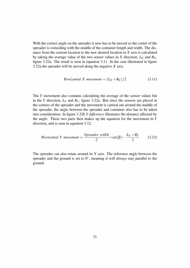
With the correct angle on the spreader it now has to be moved so the center of thespreader is coinciding with the middle of the container length and width. The dis-tance from the current location to the new desired location in X axis is calculatedby taking the average value of the two sensor values in X direction, LX and RX ,figure 3.22a. The result is seen in equation 3.11. In the case illustrated in figure3.22a the spreader will be moved along the negative X axis.

Horizontal X movement = (LX +RX)/2 (3.11)

The Y movement also contains calculating the average of the sensor values butin the Y direction, LY and RY , figure 3.22a. But since the sensors are placed inthe corners of the spreader and the movement is carried out around the middle ofthe spreader, the angle between the spreader and container also has to be takeninto consideration. In figure 3.22b Y difference illustrates the distance affected bythe angle. These two parts then makes up the equation for the movement in Ydirection, and is seen in equation 3.12.

Horizontal Y movement =Spreader width

2⇤ sin(b )� LY +RY

2(3.12)

The spreader can also rotate around its Y axis. The reference angle between thespreader and the ground is set to 0�, meaning it will always stay parallel to theground.

31

3.2.4 Simulation results

All these simulations are made with the Drop down concept.

Table 3.3 presents the time it takes to get to the goal position according to thesimulations. In simulation 0.3 m the spreader is placed 0.3 m away from its goalposition in X, Y and Z directions. The angle between the spreader and containeris 45� and the time it takes to align the spreader is 11 seconds. The slow part hereis the Y distance, the angle is great due to maximization of it within the time ittakes to align the spreader.

In 0.3m mod. the first simulation is modified to speed up the process. The X andZ distances are the same but the Y distance and the angle are tuned not to takelonger time than the X and Z movements.

For the simulation > 2 m the movements are tuned for maximum distance within9 seconds. The Z distance is greater than 2 m and when the spreader is above 2 mit is only allowed to be lowered as explained in section 3.2.3. When the spreadergets below 2 m it starts to align.

To maximize X, Y and rotation movements the Z distance is below 2 m in < 2 m.This means that X, Y and the rotation have almost 9 seconds to maximize theirmoves.

The < 2 m tele simulations are almost the same as < 2 m with only one differ-ence, the container is placed further away from the reach stacker in the X direc-tion. In the < 2 m simulations the telescopic actuator is being retracted and in< 2 m tele it is moved forward.

1 cont. and 3 cont. have the same distances to the goal position, the difference isthat in 1 cont. the stack where the container is being placed on is one containerhigh and in 3 cont. it is three containers high.

32

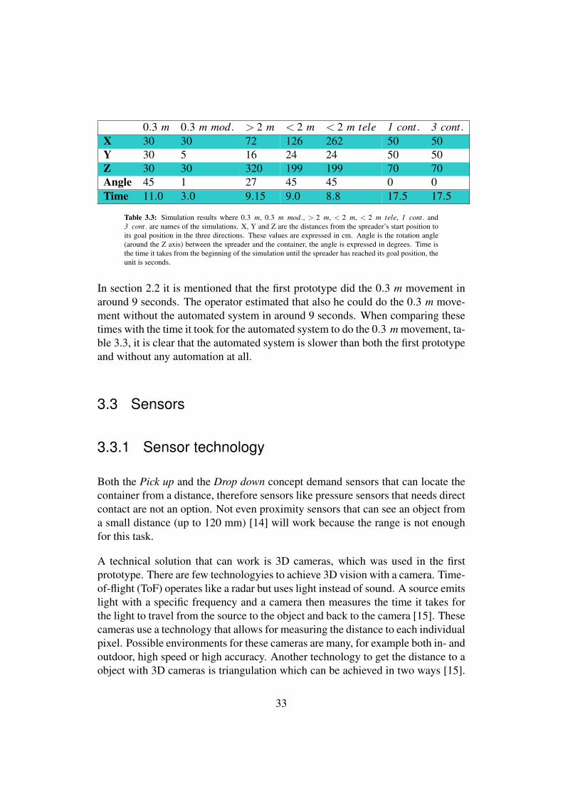
0.3 m 0.3 m mod. > 2 m < 2 m < 2 m tele 1 cont. 3 cont.X 30 30 72 126 262 50 50Y 30 5 16 24 24 50 50Z 30 30 320 199 199 70 70Angle 45 1 27 45 45 0 0Time 11.0 3.0 9.15 9.0 8.8 17.5 17.5

Table 3.3: Simulation results where 0.3 m, 0.3 m mod., > 2 m, < 2 m, < 2 m tele, 1 cont. and3 cont. are names of the simulations. X, Y and Z are the distances from the spreader’s start position toits goal position in the three directions. These values are expressed in cm. Angle is the rotation angle(around the Z axis) between the spreader and the container, the angle is expressed in degrees. Time isthe time it takes from the beginning of the simulation until the spreader has reached its goal position, theunit is seconds.

In section 2.2 it is mentioned that the first prototype did the 0.3 m movement inaround 9 seconds. The operator estimated that also he could do the 0.3 m move-ment without the automated system in around 9 seconds. When comparing thesetimes with the time it took for the automated system to do the 0.3 m movement, ta-ble 3.3, it is clear that the automated system is slower than both the first prototypeand without any automation at all.

3.3 Sensors

3.3.1 Sensor technology

Both the Pick up and the Drop down concept demand sensors that can locate thecontainer from a distance, therefore sensors like pressure sensors that needs directcontact are not an option. Not even proximity sensors that can see an object froma small distance (up to 120 mm) [14] will work because the range is not enoughfor this task.

A technical solution that can work is 3D cameras, which was used in the firstprototype. There are few technologyies to achieve 3D vision with a camera. Time-of-flight (ToF) operates like a radar but uses light instead of sound. A source emitslight with a specific frequency and a camera then measures the time it takes forthe light to travel from the source to the object and back to the camera [15]. Thesecameras use a technology that allows for measuring the distance to each individualpixel. Possible environments for these cameras are many, for example both in- andoutdoor, high speed or high accuracy. Another technology to get the distance to aobject with 3D cameras is triangulation which can be achieved in two ways [15].

33

Stereo vision, which works like our eyes. It compares differences in two picturestaken at the same time from two cameras placed next to each other and calculatesthe distance to the object from this information. The second method is using onecamera and a light projector, for example a light source that generates a dottedpattern. On a flat surface the dots will appear with a constant distance betweeneach other. On a hemisphere the space between the dots will increase the furtheraway from the center of the hemisphere they get. By measuring the distancesbetween these dots it is possible to generate a 3D image. The accuracy with thistechnology increases the nearer the camera is to the object. With a distance of0.15-0.3m the accuracy can be 10mm [16]. Several fields of view can be selected,for example 70�x52� or 45�x34� [16]. A disadvantage with 3D cameras is thatthey do not work well in fog and some cameras do not work in snow and heavyrain.

Lidar is a technology which also uses light for mapping. Lidar works like radarbut with laser instead of radio waves. It enables mapping of objects up to 100 maway with an accuracy of ±3cm [17]. This product has a vertical field of view of15� and a horizontal field of view of 360�. With this range and accuracy a set-upwith this technology has more options for placement of the sensor.

A technical solution enabling seeing through fog is ultrasonic. Ultrasonic sensorsuse the same Time-of-flight principle as the 3D camera above but with ultrasonicsound instead of light. The distance to the object is measured by the time it takesfor the sound to travel to the object and back again. This sensor set-up usuallyconsists of one transmitter and several receivers allowing for shape recognition ofthe object, different shapes and sizes gives different sensor outputs [18]. Unfor-tunately no company that sells a complete solution for this could be found, it hasto be built from scratch. However there is a company called Toposens1, which isin the process of developing a product that might work for this application. Ultra-sonic sensors usually have a beam angle between a few degrees up to 80 degrees[19].

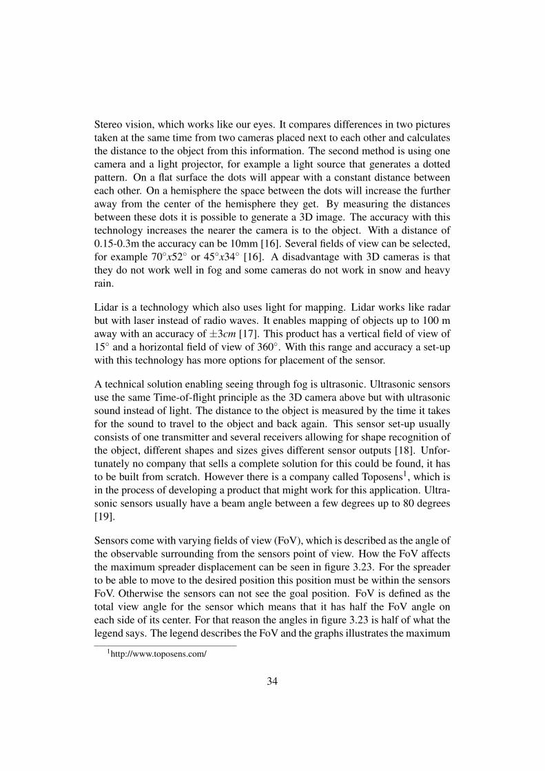
Sensors come with varying fields of view (FoV), which is described as the angle ofthe observable surrounding from the sensors point of view. How the FoV affectsthe maximum spreader displacement can be seen in figure 3.23. For the spreaderto be able to move to the desired position this position must be within the sensorsFoV. Otherwise the sensors can not see the goal position. FoV is defined as thetotal view angle for the sensor which means that it has half the FoV angle oneach side of its center. For that reason the angles in figure 3.23 is half of what thelegend says. The legend describes the FoV and the graphs illustrates the maximum

1http://www.toposens.com/

34

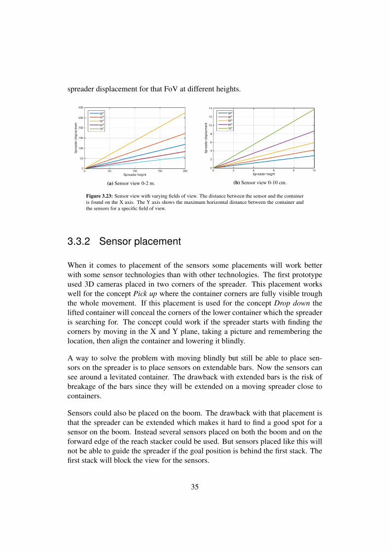
spreader displacement for that FoV at different heights.

(a) Sensor view 0-2 m. (b) Sensor view 0-10 cm.

Figure 3.23: Sensor view with varying fields of view. The distance between the sensor and the containeris found on the X axis. The Y axis shows the maximum horizontal distance between the container andthe sensors for a specific field of view.

3.3.2 Sensor placement

When it comes to placement of the sensors some placements will work betterwith some sensor technologies than with other technologies. The first prototypeused 3D cameras placed in two corners of the spreader. This placement workswell for the concept Pick up where the container corners are fully visible troughthe whole movement. If this placement is used for the concept Drop down thelifted container will conceal the corners of the lower container which the spreaderis searching for. The concept could work if the spreader starts with finding thecorners by moving in the X and Y plane, taking a picture and remembering thelocation, then align the container and lowering it blindly.

A way to solve the problem with moving blindly but still be able to place sen-sors on the spreader is to place sensors on extendable bars. Now the sensors cansee around a levitated container. The drawback with extended bars is the risk ofbreakage of the bars since they will be extended on a moving spreader close tocontainers.

Sensors could also be placed on the boom. The drawback with that placement isthat the spreader can be extended which makes it hard to find a good spot for asensor on the boom. Instead several sensors placed on both the boom and on theforward edge of the reach stacker could be used. But sensors placed like this willnot be able to guide the spreader if the goal position is behind the first stack. Thefirst stack will block the view for the sensors.

35

Lidar has a long range which makes it possible to place it on the cabin roof. Thisgives a 360� view around the vehicle, but depending on the field of view the lidarmight have to be tilted to be able to see when the spreader works high above thevehicle. This solution will not be able to see behind the first stack. In that case itis impossible for the lidar to guide the spreader.

Instead of placing sensors on the reach stacker they could be located on a drone.This could solve the drawbacks with the above mentioned placements of sensors.A drone can fly around the first stack and look from behind. A levitated containeronly blocks the view of the drone if the container is to be placed in a hole sur-rounded by containers on all sides. A drawback with a drone is the battery whichhas to be charged. But the drone will be in the air for maximum 1 minute for eachpick up and drop down, the rest of the time it can be on standby on a platform onthe reach stacker and be charged at the same time.

36

Chapter 4

Discussion and conclusions

The discussion and conclusions chapter is divided into four sections. First comesthe discussion about the concepts. Then there is a section about the Simulinkmodel, where possibilities and problems with Simulink are discussed. The thirdsection contains the discussion about sensors and their placement. The last sec-tion in this chapter is about further work.

4.1 Concept development

In section 2.1 Select Product Concepts among other topics is explained. In thiscase the selection was made as a discussion due to totally different concepts beingevaluated. In cases like this it can be a hard task to find a suitable reference conceptto which all others can be compared. When concepts such as Warning system isevaluated against Spreader height it is difficult to find a suitable reference object.That is why there was a discussion around the concepts instead.

The concept Automated driving was eliminated since it was not suited for automa-tion. But by making it a guiding system instead of automated one there would notbe any safety risks. This guiding system could show a live feed of the upcom-ing road on a screen, and on the same screen the direction of the vehicle and themost favourable route are also displayed. Today rear view cameras work similarto this with the exception that no route is proposed. Maybe such a system wouldnot be used every time but it could work as a training system for new operators.However, the development of such a guiding system would probably be time con-

37

suming so it might not be worth it if the system would not be used on a daily basis.On the other hand a guiding system would be a perfect evaluation of a possibleAutomated driving concept.

One of the research questions was Which areas would benefit most from driverassistance? As described in section 3.1 Pick up and Drop down are the mostpromising concepts. If the sensor placement is also considered Pick up standsout as a winner. Drop down absolutely has potential but the sensor placement forthat concept is more difficult. The concept Spreader hight also has potential ifthe hight of the stack is known in the container information system. If it shouldrely only on sensors it would probably be too slow from time to time, for examplewhen the spreader can not see the stack in time for it to be raised before the vehiclereaches the stack. This concept does however not require any simulations becauseit is a relatively easy task. The equations used in Lower Z1 in section 3.2.3 can beused for this movement as well.

4.2 Simulink model

A lot of time during this project went into the building of the model, both in thebuilding itself but also in the understanding of Simulink. The author had onlyused Simulink once before starting this project and that time he got a finishedmodel and only did tests with it. When the understanding of the program grewthe possibilities seem endless. The author believes that if there was more time areach stacker model could be built in Simulink for testing nearly every part of thevehicle, not only the hydraulic lifting system.

A problem that arose during the building of the Simulink model had to do withthe actuators. The mechanical part of the actuator adapts itself to the startingposition of the simulations. This means that the mechanical part of the actuatorwhich levitates the boom will be more extended in the beginning of the simulationif the spreader’s start position is high up, than if it was close to the ground. Butunfortunately the hydraulic part of the actuator did not extend and this could notbe seen in the compiled simulation. Suddenly the actuator did just stop for noapparent reason. A lot of thought and time were required to realize where theproblem was.

While tuning the speeds for the actuators, see table 2.1, to correspond with realitythe hydraulic parameters for the actuators were changed. The final parametervalues did not have anything to do with reality instead they assured the speeds

38

were correct. The size off the hydraulic pump was not taken into considerationwhile tuning the parameters and the motor that drives the pump in the model has aconstant rpm. In reality the rpm is adapted to the real time need of the pump. Theonly constraints for the pump was the maximum pressure of 245 bar, see section2.2. It might be that the pump in the model is too big and that in reality it cannot handle all the actuators moving at the same time. That is something that hasto be further investigated. This simplification in the model was made due to timeconstraints.

When tuning the hydraulic actuators there are a lot of parameters to take intoconsideration, described in section 3.2.2. One of these is how the actuators af-fects each other. Figure 3.17a shows the measured values from the rotary and thespreader width actuators. Both signals oscillates in the beginning. The movementscreated from these oscillations are very small, in the range of ±0.0002 m for thespreader width actuator and ±0.0006 degrees for the rotary actuator. These move-ments will therefore not be possible to detect with the naked eye so from that pointof view the oscillations must not be removed since the values converges. However,these oscillations will possibly result in a marginally slower automated process,but the most important reason to remove the oscillations is the simulation time.When building a model like this there will be a lot of testing with different valuesfor all parameters. Long simulation times because of unnecessary oscillations willlead to increased work time, therefore this tuning is important to do before time iswasted on long simulations.

Some times even the lack of control can be of help. To make the rotary actuatormove in a linear fashion it is set to a goal position of -1000 or 1000 degrees whenit does big movements, see section 3.2.2 about control results. The PI controller isonly in use when the rotary actuator is within three degrees from its goal position.This is not how the rotary actuator was intended to be designed, the plan wasto always go through the controller. However, when always going through thecontroller the rotary actuator did not work for both small and big rotations. Thissolution makes it linear but might not be the most elegant solution. The angleof 1000 was chosen due to the big number, the actuator will never get close tothe angle and therefore not slow down for other reasons than the approach of thereference value.

The time it takes for a actuator to complete its movement depends on its speed andthe control output. The combined movement pattern for the actuators is not linear.If several actuators move at the same time the fastest will complete its movementfirst. That means that when lowering the spreader it might look like it changesthe X coordinate as well because the boom telescope actuator might be moving

39

slower than the boom lift actuator. It is due to that the actuators are always movingat their highest speed and that could be a problem. If a container is to be placedin an area surrounded by other containers there might not be much room to playwith and the movement has to be linear. A solution to this is calculating the timeevery actuator will need and adjust the speed of the faster actuators to the one thatneeds the most time.

When building this model the author used a substitute for the sensors. Insteadof sensors the model measures the exact distance between the container placedon the ground and points fixed to the spreader. This is what a sensor would alsodo but in another way. In the Pick up concept simulation these fixed points aretwo corners of the spreader and for the Drop down concept the fixed points arelocated on two corners of the container. Since this is done in Matlab the distancemeasurement will be exact and the sensors can therefore be seen as ideal, whichwill not be the case for a real product. Bad sensor resolution could be a problemwhich is not considered in the simulations, more about that in section 4.3. It isalso assumed that both sensors can see the container castings which does not needto be the case and it does not need to be a problem either. It could be solvedwith clever programming. If one sensor sees a corner and the other does not seeanything the spreader can be moved just from the angles of the corner that is seen.If the angle between the container corner and the spreader is large, the spreaderhas to be rotated for the other sensor to be able to see its corner. If the spreaderangle is near zero, relative to the container, the spreader must be moved sideways.

For the evaluation of the simulations the author chose to use the Drop down con-cept. This concept is the most demanding for the system since it lifts a heavycontainer that weighs up to 45 ton. While tuning the speeds for the actuators theslowest times was chosen, in other words, the time it takes to move the actuatorwhen it is under the greatest strain.

One of the research questions that was presented in the beginning of the reportwas What kind of control is needed for these systems? In section 3.2.2 about thecontrol it is stated that none of the controllers use a derivative gain and only a smallintegral gain is used. No fuzzy controller was actually tested because there wasno need for it. The only controller which is a bit special is the rotary controller.It uses two different controllers depending on if the -1000/1000 reference angle isused or not. If it is used the controller is a bit weaker than if it is not used. Theauthor believe a lot of this has to do with the proportional valve. If a classic on/offvalve is used instead it would put higher demands on the controller.

40

Another research questions was Can an automated system with this setup be fasterthan a human operator? As can be read in table 2.1 about the actuator speeds theSpreader sideshift moves ±800 mm in < 26 seconds or ⇡ 3 cm/second. This datais taken from appendix B.2. However, when this was presented for the peopleat Konecranes they said that the spreader moved with a speed of 10 cm/secondin that direction. If this is true the time for the 0.3 m simulation presented intable 2.1 be just over 3 seconds, if the angle of 45� is reduced. This would bea big improvement of the process. Before this information was revealed fromKonecranes the author thought was to recommend them to talk to Elme aboutmaking the Spreader sideshift movement faster because it had an negative impacton the process. Unfortunately was the information in Elme’s brochure trusted andthe new information from Konecranes came after the work was finished, there-fore the simulations are not updated with the correct speed. But if this is takeninto consideration while discussing the simulation times in table 2.1 the resultsare very satisfying. The distance that in the first prototype took approximately9 seconds takes just over 3 seconds with concurrent movements. In simulation< 2m tele when the concurrent movement takes 9 seconds it can move approx-imately 260 cm in X direction, 200 cm in Z direction and rotate 45�. If the Xdistance travelled within 9 seconds also is calculated with the new speed it gets10[cm/second]⇤9[seconds] = 90[cm] instead of 24 cm. It can also be seen, if wecompare simulation 1 cont. with 3 cont., that the height of the spreader would notchange the times.

4.3 Sensors

As mentioned in the target specifications, section 3.1.3, the alignment must bewithin 5 cm for a perfect alignment to work. In the section about sensor technol-ogy, section 3.3.1, resolutions for a few sensors using different technologies arepresented. All these resolutions are within 5 cm when the sensor gets close to theobject but some of them might not have high enough resolution if they are scan-ning the environment from a distance. This has to be considered while decidingsensor technology and placement.

In section 3.1.2 about customer needs it is mentioned that robustness is an impor-tant feature of a system like this. The author believes that the hardest obstacle toachieve this is the sensors. The environment in which the reach stackers will workcan be harsh. The equipment will be exposed to heavy rain, fog, snow and coldweather which can have an impact on the accuracy of the sensors. Furthermore

41

the placement also affects the robustness. Under the category Robust in table 3.1it can be seen that the customer statement Reliable is translated to the customerneed Can be repeated without any problems. This means that the system shouldalways work. When it comes to sensor placement this customer need might behard to fulfil. The sensor placement will influence which container placement ispossible for the system to handle. For example a Lidar placed on the cabin roofwill not allow for drop down and pick up behind the first stack. Therefore find-ing a good sensor placement and a matching sensor for that placement will be acrucial part in further development of this system.

With the robustness in mind the authors personal favourite for the sensor place-ment is the drone. The reason for that is the versatility of the drone. Dependingon if the chosen container is in the first or the second stack, if it stands on theground or 4 containers up the drone can hover in different positions. The droneconcept is probably the concept which demands most pre-work since it has to beprogrammed and tested for several positions. Another concept that could fulfil therobustness need is sensors placed on the spreader that takes a picture and movesblindly when a levitated container is blocking the view of the final position. Thissolution sets high requirements on the system by not having any real time feed-back of the distances to the goal position. A third possible solution is to combineseveral sensor placements and using different sensors depending on the locationof the spreader.

4.4 Further work

There is still a long way to go before this system can be implemented on a realreach stacker. The author’s recommendation is to start with getting all of theparameters right in the model and not just have the speeds and pressure as limits.By doing so there will be more understanding of the pump’s possibilities. If thepump can handle movements from all actuators at the same time or if the speedswill be lowered.

Sensors in the model could also be designed to mimic how they work in the realworld. The sensor field of view affects how far away from the container, in the Xand Y plan, the sensors can be and still see the container castings. By implement-ing a sensor field of view in the model the largest spreader displacement could betested. It might also be possible to add a filter on the sensors which allows for testof the sensor accuracy. In the model used for this thesis work the sensors measurethe distance between the spreader and the container or between the container and

42

the container, which a real sensor also would do. But this model does not carewhere the sensor is placed, it only uses these values which the real sensor wouldsend to the system. The sensor placement could also be tested in the model, tobetter see the affect of the sensor shadow.

Sensors should also be tested in the physical world, not only in the Simulinkmodel. Testing different sensors and placement will give a greater understandingof what is possible with the different techniques. If the choice is to use a dronethat work itself could be an exciting MSc thesis.

43

Bibliography

[1] Konecranes. NearGuard system for konecranes lifttrucks. Brochure. Lastvisited 18 February 2016. URL: http : / / www . kclifttrucks . com /

sites/lifttrucks/files/download/nearguard_rfid-customer_

leaflet.pdf.

[2] Konecranes. Remote monitoring for lift trucks. Brochure. Last visited 18February 2016. 2014. URL: http://www.kclifttrucks.com/sites/lifttrucks/files/download/kc_truconnect_for_lifttrucks_

brochure_2.0.pdf.

[3] Associated Press in Detroit. Tesla’s new autopilot system lets electric carchange lanes by itself. Published 15 October 2015. The Guardian. URL:http://www.theguardian.com/technology/2015/oct/15/teslas-

new-autopilot-system-lets-electric-car-change-lanes-by-

itself.

[4] James Marek. Hydraulic vs. Electromechanical Actuators. Article. Pub-lished 9 April 2012, last visited 3 August 2016. URL: http : / / www .mbtmag.com/article/2012/05/hydraulic-vs-electromechanical-

actuators.

[5] Lane Desborough and Randy Miller. “Increasing Customer Value of Indus-trial Control Performance Monitoring—Honeywell’s Experience”. In: SixthInternational Conference on Chemical Process Control AIChE SympoisumSeries Number 326 (Vol. 98) (2002).

[6] Le Duc Hanh, Kyoung Kwan Ahn, Nguyen Bao Kha, and Woo Keun Jo.“Trajectory control of electro-hydraulic excavator using fuzzy self tuningalgorithm with neural network”. In: Journal of Mechanical Science andTechnology 23 (2009), pp. 149 –160.

44

[7] Li Bo, Yan Jun, Guo Gang, Zeng Yonghua, and Luo Wenxing. “High Per-formance Control of Hydraulic Excavator Based on Fuzzy-PI Soft-SwitchController”. In: Computer Science and Automation Engineering 2 (2011),pp. 676 –679.

[8] Karl T. Ulrich and Steven D. Eppinger. Produktutveckling, Original ti-tle: Produc Design and Development. Swedish. Trans. fromEnglish byRobert Bjarnemo, Damien Motte, and Silvia Bentsson. Studentlitteratur,Lund, Sweden, 2014. ISBN: 9789144074214.

[9] Matlab. Simulation and Model-Based Design. Last visited 4 August 2016.URL: http://se.mathworks.com/products/simulink/.

[10] Matlab. The Language of Technical Computing. Last visited 4 August 2016.URL: http://se.mathworks.com/products/matlab/.

[11] Matlab. Model and simulate multidomain physical systems. Last visited 4August 2016. URL: http://se.mathworks.com/products/simscape/.

[12] Karl Johan Astrom and Richard M. Murray. Feedback Systems. PrincetonUniversity Press, New Jersey, USA, 2008. ISBN: 9780691135762.

[13] Matlab. Model and simulate decision logic using state machines and flowcharts. Last visited 8 August 2016. URL: http://se.mathworks.com/products/stateflow/.

[14] Balluff. Inductive sensor. Brochure. Last visited 1 July 2016. URL: http://www.balluff.com/balluff/MUS/en/products/product_detail.

jsp#/132238.[15] Fotonic. The importance of the third dimension. Brochure. Last visited 3

July 2016. 2015. URL: http://www.fotonic.com/technology/.[16] Fotonic. Smart 3D-Cameras. Brochure. Last visited 3 July 2016. 2015.

URL: http://www.fotonic.com/wp-content/uploads/2015/10/Datasheet_Fotonic_E-series_2015_1-2.pdf.

[17] Velodyne. Velodyne LiDAR PUCK. Brochure. Last visited 4 July 2016.URL: http://velodynelidar.com/docs/datasheet/63-9229_Rev-C_VLP16_Datasheet_Web.pdf.

[18] Kozo Ohtani and Mitsuru Baba. “Shape Recognition and Position Measure-ment of an Object Using an Ultrasonic Sensor Array”. In: Sensor Array. Ed.by Prof. Wuqiang Yang. Available from: http://www.intechopen.com/books/sensor-array/shape-recognition-and-position-measurement-of-anobject-using-an-ultrasonic-sensor-array. InTech, 2012. Chap. 4, pp. 53–66.

[19] Murata. MA40S4S. Last visited 9 August 2016. URL: http://www.murata.com/en-eu/products/productdetail?partno=MA40S4S.

45

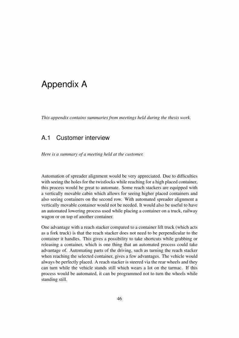
Appendix A

This appendix contains summaries from meetings held during the thesis work.

A.1 Customer interview

Here is a summary of a meeting held at the customer.

Automation of spreader alignment would be very appreciated. Due to difficultieswith seeing the holes for the twistlocks while reaching for a high placed container,this process would be great to automate. Some reach stackers are equipped witha vertically movable cabin which allows for seeing higher placed containers andalso seeing containers on the second row. With automated spreader alignment avertically movable container would not be needed. It would also be useful to havean automated lowering process used while placing a container on a truck, railwaywagon or on top of another container.

One advantage with a reach stacker compared to a container lift truck (which actsas a fork truck) is that the reach stacker does not need to be perpendicular to thecontainer it handles. This gives a possibility to take shortcuts while grabbing orreleasing a container, which is one thing that an automated process could takeadvantage of. Automating parts of the driving, such as turning the reach stackerwhen reaching the selected container, gives a few advantages. The vehicle wouldalways be perfectly placed. A reach stacker is steered via the rear wheels and theycan turn while the vehicle stands still which wears a lot on the tarmac. If thisprocess would be automated, it can be programmed not to turn the wheels whilestanding still.

46

A system like this must always work, independently of weather and light, if itonly works 80% of the time the operator will not use it. If it for some reasondoes not work or can not continue with a started task, the system needs to tell theoperator about this. The time for a specific movement does not need to be fasterthan with manual steering, but the time for the whole process does, regardless ifthe automated system is kinder to the equipment. This means that an automatedsystem that is cheaper to use compared to a manual movement due to lower wearand tear but is slower than the manual movement will not be used by the operator.

An important thing that has to be considered while designing a system like thisis safety. Making the reach stacker drive in automatic mode puts a whole newlevel of safety risks to the process. A self driving vehicle takes the legal respon-sibility away from the operator, leading to a higher safety level required on thearea where the vehicle is used, which in turns leads to a higher investment. Thiscould however work, but it is a much bigger concept than automating parts of areach stacker and use it in the same safety areas as to today. By letting the parkingbreak be activated while in automated mode there would not be a requirement ona higher safety level on the operating area.

The operator has to be able to stop and terminate the process, but there is no needfor the operator to be able to decide the speed or direction of the movements.The process could be started with a button and the process could be stopped whencompleted or when the operator moves anything. Allowing the operator to stop theprocess by moving anything and not demanding a stop button push is a much safersolution. In a situation where a fast decision is crucial it should be easy to stopthe movement. Even though the system can work on its own when started somesensors guaranteeing that the operator still is in the seat is required. There shouldnot be any reason to give the operator a lot of information while the automatedsystem is active, except a light indicating that the system is working. If the sensorslose contact with the container the light will be turned off. On the existing reachstackers today, there is a light turned on when the twistlocks are in place, thiswould be enough even for indicating that the automated process is finished. If anerror occurs, like sensors losing connection with the container, an error messagetells the driver about the error.

47

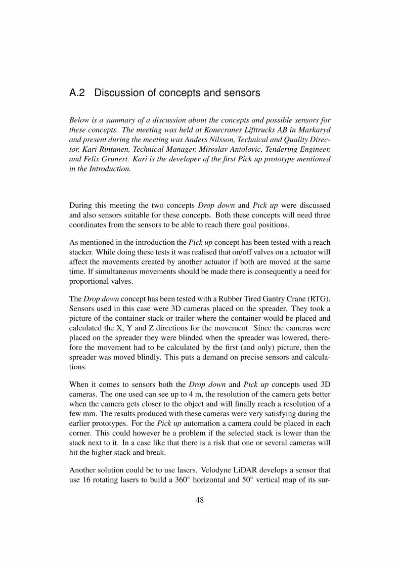
A.2 Discussion of concepts and sensors

Below is a summary of a discussion about the concepts and possible sensors forthese concepts. The meeting was held at Konecranes Lifttrucks AB in Markarydand present during the meeting was Anders Nilsson, Technical and Quality Direc-tor, Kari Rintanen, Technical Manager, Miroslav Antolovic, Tendering Engineer,and Felix Grunert. Kari is the developer of the first Pick up prototype mentionedin the Introduction.

During this meeting the two concepts Drop down and Pick up were discussedand also sensors suitable for these concepts. Both these concepts will need threecoordinates from the sensors to be able to reach there goal positions.

As mentioned in the introduction the Pick up concept has been tested with a reachstacker. While doing these tests it was realised that on/off valves on a actuator willaffect the movements created by another actuator if both are moved at the sametime. If simultaneous movements should be made there is consequently a need forproportional valves.

The Drop down concept has been tested with a Rubber Tired Gantry Crane (RTG).Sensors used in this case were 3D cameras placed on the spreader. They took apicture of the container stack or trailer where the container would be placed andcalculated the X, Y and Z directions for the movement. Since the cameras wereplaced on the spreader they were blinded when the spreader was lowered, there-fore the movement had to be calculated by the first (and only) picture, then thespreader was moved blindly. This puts a demand on precise sensors and calcula-tions.

When it comes to sensors both the Drop down and Pick up concepts used 3Dcameras. The one used can see up to 4 m, the resolution of the camera gets betterwhen the camera gets closer to the object and will finally reach a resolution of afew mm. The results produced with these cameras were very satisfying during theearlier prototypes. For the Pick up automation a camera could be placed in eachcorner. This could however be a problem if the selected stack is lower than thestack next to it. In a case like that there is a risk that one or several cameras willhit the higher stack and break.

Another solution could be to use lasers. Velodyne LiDAR develops a sensor thatuse 16 rotating lasers to build a 360� horizontal and 50� vertical map of its sur-

48

roundings. The sensor resolution is ±2 cm and it costs around 9 000 $.

Not all containers have the same height, so this can not be hardcoded. Whenplacing a container on a stack or trolley the height must be a known parameter.This could be achieved by measuring the hight of a container while handling it,but that is harder than it sounds. If it is picked up from a stack there is no goodreference point to measure from if the cameras are placed on the spreader. Sensorscould be placed on the boom but then the question is were on the boom to placeit since the boom can be extended. Today, well-organised harbours have systemsknowing where all containers are placed and also its measurements. In the futureall harbours will have systems like this and then no real time measuring of thecontainer height will be needed.

49

Appendix B

This appendix consists of parts of brochures containing data of dimensions andspeeds used for the model.

B.1 Konecranes, Reach Stacker

This section contains three pages from a brochure about Konecranes reach stack-ers. The selected pages have information about the dimensions of the reach stack-ers. The reach stacker used as a model for this project is SMV 4535 TB51.

1Konecranes. Reach stackers with heart. Last visited 17 September 2016. Page 19- 21. URL: http://www.konecranes.com/sites/default/files/download/kc_rst_

print_8809022_low.pdf

50

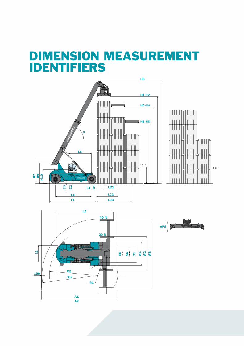
MODEL SMV 108 – 2518

Transmission UnitsMake DANA ZFModel TE-17300 4WG-191Gear shift type Automatic AutomaticNo. of gears (fwd / rev) No. 3 / 3 4 / 3Power rating (max) kW 200 200

MODEL SMV 4127 - 4545 TBX5 to SMV 4123 - 4545 CBX5

Engine UnitsMake Volvo Scania Scania Cummins Volvo Scania Volvo ScaniaModel TAD-1340-VE DC-13-074 DC-13-076 QSM-11-C335 TAD-1360-VE DC-13-081 TAD-1361-VE DC-13-077Emission approval, EU / US St 2 / Tier 2 St 2 / Tier 2 St 3a / Tier 3 St 3a / Tier 3 St 3b / Tier 4i St 3b / Tier 4i St 3b / Tier 4i St 3b / Tier 4iPower / max speed (ISO 3046) kW/rpm 256 / 2100 257 / 2100 257 / 2100 272 / 2100 256 / 1900 257 / 2100 285 / 1900 294 / 2100Torque @ speed (ISO 3046) Nm/rpm 1770 / 1250 1950 / 1200 1640 / 1400 1674 / 1000 1740 / 1200 1950 / 1200 1940 / 1000 2172 / 1200Displacement / cylinders L/-- 12.8 / 6-cyl 12.7 / 6-cyl 12.7 / 6-cyl 10.8 / 6-cyl 12.8 / 6-cyl 12.7 / 6-cyl 12.8 / 6-cyl 12.7 / 6-cylAlternator power / capacity W/Amp 3080 / 110 2800 / 100 2800 / 100 1960 / 70 3080 / 110 2800 / 100 3080 / 110 2800 / 100Fuel consumption (normal) L/hour 12-16 12-16 12-16 12-16 12-16 12-16 14-20 14-20

Transmission (make / model) DANA TE-27 DANA TE-27 DANA TE-27 DANA TE-27 DANA TE-27 (opt. ZF 4WG-261)

DANA TE-27 (opt. ZF 4WG-261) DANA TE-32 DANA TE-32

DIMENSION MEASUREMENT IDENTIFIERS

H7

H9

H10

C3

C2

L3

L1

L4 C1 LC1

LC2

LC3

L5

H8

H1-H2

H3-H4

H5-H6

±PS

T2

100R3

R2

R1

A1A2

L2

40 ft

20 ft

SS

SR T1 W1

W2

W3

9'6"8’6”

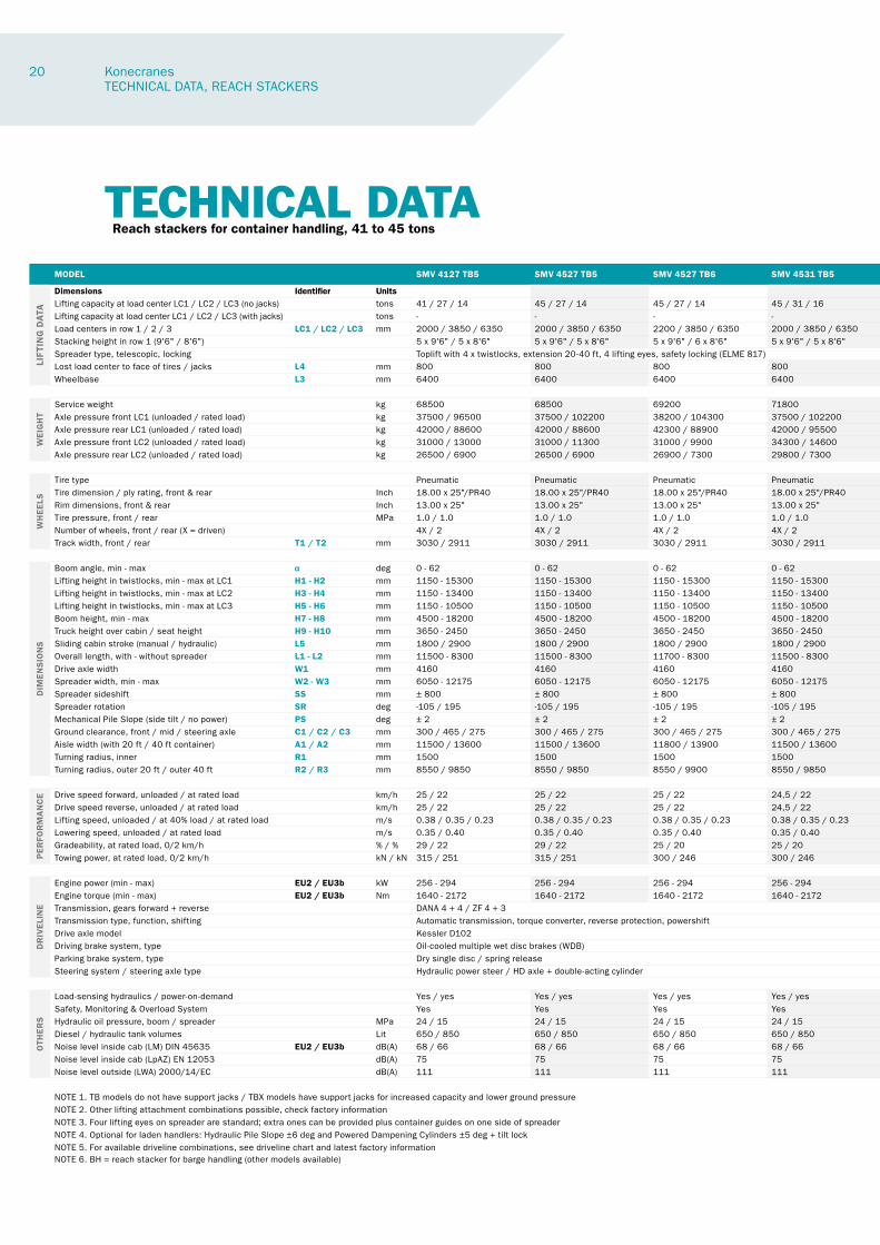
TECHNICAL DATA Reach stackers for container handling, 41 to 45 tons

MODEL SMV 4127 TB5 SMV 4527 TB5 SMV 4527 TB6 SMV 4531 TB5 SMV 4531 TB6 SMV 4535 TB5 (TBX5) SMV 4537 TB5 (TBX5) SMV 4542 TB5 (TBX5) SMV 4543 TB5 (TBX5) SMV 4545 TB5 (TBX5) SMV 4545 TB3 (BH)

LIFT

ING

DAT

A

Dimensions Identifier UnitsLifting capacity at load center LC1 / LC2 / LC3 (no jacks) tons 41 / 27 / 14 45 / 27 / 14 45 / 27 / 14 45 / 31 / 16 45 / 31 / 16 45 / 35 / 20 45 / 37 / 19 45 / 42 / 24 45 / 42 / 25 45 / 45 / 37 45 / 45 / 35Lifting capacity at load center LC1 / LC2 / LC3 (with jacks) tons - - - - - 45 / 37 / 24 45 / 41 / 28 45 / 44 / 30 45 / 44 / 34 45 / 45 / 45 45 / 45 / 35Load centers in row 1 / 2 / 3 LC1 / LC2 / LC3 mm 2000 / 3850 / 6350 2000 / 3850 / 6350 2200 / 3850 / 6350 2000 / 3850 / 6350 2200 / 3850 / 6350 1900 / 3850 / 6350 2000 / 3850 / 6350 1800 / 3850 / 6350 1800 / 3850 / 6350 2275 / 3850 / 6350 1975 / 3875 / 6375Stacking height in row 1 (9'6" / 8'6") 5 x 9'6" / 5 x 8'6" 5 x 9'6" / 5 x 8'6" 5 x 9'6" / 6 x 8'6" 5 x 9'6" / 5 x 8'6" 5 x 9'6" / 6 x 8'6" 5 x 9'6" / 5 x 8'6" 5 x 9'6" / 5 x 8'6" 5 x 9'6" / 5 x 8'6" 5 x 9'6" / 5 x 8'6" 5 x 9'6" / 5 x 8'6" 3 x 9'6" / 3 x 8'6"Spreader type, telescopic, locking Toplift with 4 x twistlocks, extension 20-40 ft, 4 lifting eyes, safety locking (ELME 817) Lost load center to face of tires / jacks L4 mm 800 800 800 800 800 930 930 930 930 1025 1025Wheelbase L3 mm 6400 6400 6400 6400 6400 6400 6400 7250 7500 8000 9000

WEI

GH

T

Service weight kg 68500 68500 69200 71800 72500 79700 83000 83500 84500 107000 105200Axle pressure front LC1 (unloaded / rated load) kg 37500 / 96500 37500 / 102200 38200 / 104300 37500 / 102200 38200 / 104300 38700 / 103400 42000 / 106700 42000 / 104400 42500 / 103700 51000 / 114600 52000 / 118300Axle pressure rear LC1 (unloaded / rated load) kg 42000 / 88600 42000 / 88600 42300 / 88900 42000 / 95500 42300 / 95800 43400 / 104400 46500 / 110100 46400 / 116000 47100 / 116000 54600 / 127200 57300 / 121200Axle pressure front LC2 (unloaded / rated load) kg 31000 / 13000 31000 / 11300 31000 / 9900 34300 / 14600 34300 / 13200 41000 / 21300 41000 / 21300 41500 / 24100 42000 / 25800 56000 / 37400 53200 / 31900Axle pressure rear LC2 (unloaded / rated load) kg 26500 / 6900 26500 / 6900 26900 / 7300 29800 / 7300 30200 / 7700 36300 / 10300 36500 / 9900 37100 / 9500 37400 / 10500 52400 / 24800 47900 / 20100

WH

EELS

Tire type Pneumatic Pneumatic Pneumatic Pneumatic Pneumatic Pneumatic Pneumatic Pneumatic Pneumatic Pneumatic PneumaticInch 18.00 x 25"/PR40 18.00 x 25"/PR40 18.00 x 25"/PR40 18.00 x 25"/PR40 18.00 x 25"/PR40 18.00 x 33"/PR36 18.00 x 33"/PR36 18.00 x 33"/PR36 18.00 x 33"/PR36 21.00x35"/PR40 21.00 x 35"/PR40Inch 13.00 x 25" 13.00 x 25" 13.00 x 25" 13.00 x 25" 13.00 x 25" 13.00 x 33" 13.00 x 33" 13.00 x 33" 13.00 x 33" 15.00 x 35" 15.00 x 35"

Tire pressure, front / rear MPa 1.0 / 1.0 1.0 / 1.0 1.0 / 1.0 1.0 / 1.0 1.0 / 1.0 1.0 / 1.0 1.0 / 1.0 1.0 / 1.0 1.0 / 1.0 1.0 / 1.0 1.0 / 1.0Number of wheels, front / rear (X = driven) 4X / 2 4X / 2 4X / 2 4X / 2 4X / 2 4X / 2 4X / 2 4X / 2 4X / 2 4X / 2 4X / 2Track width, front / rear T1 / T2 mm 3030 / 2911 3030 / 2911 3030 / 2911 3030 / 2911 3030 / 2911 3030 / 2911 3030 / 2911 3030 / 2911 3030 / 2911 3227 / 3420 3227 / 3420

DIM

ENS

ION

S

Boom angle, min - max deg 0 - 62 0 - 62 0 - 62 0 - 62 0 - 62 0 - 62 0 - 62 0 - 61 0 - 59 0 - 55 0 - 62Lifting height in twistlocks, min - max at LC1 H1 - H2 mm 1150 - 15300 1150 - 15300 1150 - 15300 1150 - 15300 1150 - 16300 1300 - 15400 1300 - 15400 1300 - 15400 1300 - 15400 1300 - 15400 1300 - 15400Lifting height in twistlocks, min - max at LC2 H3 - H4 mm 1150 - 13400 1150 - 13400 1150 - 13400 1150 - 13400 1150 - 14200 1300 - 13500 1300 - 13500 1300 - 13500 1300 - 13500 1300 - 14600 1300 - 13500Lifting height in twistlocks, min - max at LC3 H5 - H6 mm 1150 - 10500 1150 - 10500 1150 - 10500 1150 - 10500 1150 - 11500 1300 - 10500 1300 - 10600 1300 - 10400 1300 - 10400 1300 - 11600 1300 - 10500Boom height, min - max H7 - H8 mm 4500 - 18200 4500 - 18200 4500 - 18200 4500 - 18200 4500 - 19300 4675 - 18350 4775 - 18400 4775 - 18500 4975 - 18500 5100 - 18800 4675 - 18300Truck height over cabin / seat height H9 - H10 mm 3650 - 2450 3650 - 2450 3650 - 2450 3650 - 2450 3650 - 2450 3800 - 2650 3800 - 2650 3800 - 2650 3800 - 2650 4050 - 2900 3800 - 2650Sliding cabin stroke (manual / hydraulic) L5 mm 1800 / 2900 1800 / 2900 1800 / 2900 1800 / 2900 1800 / 2900 1800 / 2900 1800 / 2900 1800 / 2900 1800 / 2900 1800 / 2900 1800 / 2900Overall length, with - without spreader L1 - L2 mm 11500 - 8300 11500 - 8300 11700 - 8300 11500 - 8300 11700 - 8300 11500 - 8450 11500 - 8450 12300 - 9300 12550 - 9550 14150 - 10600 11500 - 8450Drive axle width W1 mm 4160 4160 4160 4160 4160 4160 4160 4160 4160 4600 4160Spreader width, min - max W2 - W3 mm 6050 - 12175 6050 - 12175 6050 - 12175 6050 - 12175 6050 - 12175 6050 - 12175 6050 - 12175 6050 - 12175 6050 - 12175 6050 - 12175 6050 - 12175Spreader sideshift SS mm ± 800 ± 800 ± 800 ± 800 ± 200 ± 800 ± 800 ± 800 ± 800 ± 800 ± 800Spreader rotation SR deg -105 / 195 -105 / 195 -105 / 195 -105 / 195 ± 200 -105 / 195 -105 / 195 -105 / 195 -105 / 195 -105 / 195 -105 / 195Mechanical Pile Slope (side tilt / no power) PS deg ± 2 ± 2 ± 2 ± 2 ± 5 ± 2 ± 2 ± 2 ± 2 ± 2 ± 2Ground clearance, front / mid / steering axle C1 / C2 / C3 mm 300 / 465 / 275 300 / 465 / 275 300 / 465 / 275 300 / 465 / 275 300 / 465 / 275 300 / 425 / 450 300 / 425 / 450 300 / 425 / 450 300 / 425 / 450 300 / 300 / 500 300 / 300 / 500Aisle width (with 20 ft / 40 ft container) A1 / A2 mm 11500 / 13600 11500 / 13600 11800 / 13900 11500 / 13600 11800 / 13900 11500 / 13600 11500 / 13600 12650 / 13850 12900 / 14000 15200 / 15400 15900 / 15900Turning radius, inner R1 mm 1500 1500 1500 1500 1500 1500 1500 2200 2600 2800 3250Turning radius, outer 20 ft / outer 40 ft R2 / R3 mm 8550 / 9850 8550 / 9850 8550 / 9900 8550 / 9850 8550 / 9900 8550 / 9850 8550 / 9850 9750 / 10400 10100 / 10750 11300 / 11300 12400 / 12400

PER

FOR

MA

NC

E Drive speed forward, unloaded / at rated load km/h 25 / 22 25 / 22 25 / 22 24,5 / 22 24,5 / 22 26 / 23 25 / 22,5 25 / 22,5 25 / 22,5 24 / 20 24 / 20Drive speed reverse, unloaded / at rated load km/h 25 / 22 25 / 22 25 / 22 24,5 / 22 24,5 / 22 26 / 23 25 / 22,5 25 / 22,5 25 / 22,5 24 / 20 24 / 20Lifting speed, unloaded / at 40% load / at rated load m/s 0.38 / 0.35 / 0.23 0.38 / 0.35 / 0.23 0.38 / 0.35 / 0.23 0.38 / 0.35 / 0.23 0.38 / 0.35 / 0.23 0.38 / 0.35 / 0.23 0.38 / 0.35 / 0.23 0.38 / 0.35 / 0.23 0.37 / 0.34 / 0.22 0.35 / 0.33 / 0.17 0.35 / 0.33 / 0.17Lowering speed, unloaded / at rated load m/s 0.35 / 0.40 0.35 / 0.40 0.35 / 0.40 0.35 / 0.40 0.35 / 0.40 0.35 / 0.40 0.35 / 0.40 0.35 / 0.40 0.35 / 0.40 0.25 / 0.35 0.25 / 0.35Gradeability, at rated load, 0/2 km/h % / % 29 / 22 29 / 22 25 / 20 25 / 20 25 / 20 24 / 18 24 / 18 23 / 17 23 / 17 22 / 16 22 / 16Towing power, at rated load, 0/2 km/h kN / kN 315 / 251 315 / 251 300 / 246 300 / 246 300 / 246 260 / 214 260 / 214 260 / 214 260 / 214 260 / 214 260 / 214

DR

IVEL

INE

Engine power (min - max) EU2 / EU3b kW 256 - 294 256 - 294 256 - 294 256 - 294 256 - 294 256 - 294 256 - 294 256 - 294 256 - 294 256 - 294 256 - 294Engine torque (min - max) EU2 / EU3b Nm 1640 - 2172 1640 - 2172 1640 - 2172 1640 - 2172 1640 - 2172 1640 - 2172 1640 - 2172 1640 - 2172 1640 - 2172 1640 - 2172 1640 - 2172Transmission, gears forward + reverse DANA 4 + 4 / ZF 4 + 3Transmission type, function, shifting Automatic transmission, torque converter, reverse protection, powershiftDrive axle model Kessler D102 Kessler D106 Kessler D111 Kessler D111Driving brake system, type Oil-cooled multiple wet disc brakes (WDB)Parking brake system, type Dry single disc / spring releaseSteering system / steering axle type Hydraulic power steer / HD axle + double-acting cylinder

OTH

ERS

Load-sensing hydraulics / power-on-demand Yes / yes Yes / yes Yes / yes Yes / yes Yes / yes Yes / yes Yes / yes Yes / yes Yes / yes Yes / yes Yes / yesYes Yes Yes Yes Yes Yes Yes Yes Yes Yes Yes

Hydraulic oil pressure, boom / spreader MPa 24 / 15 24 / 15 24 / 15 24 / 15 24 / 15 24 / 15 24 / 15 25 / 15 25 / 15 24 / 15 24 / 15Diesel / hydraulic tank volumes Lit 650 / 850 650 / 850 650 / 850 650 / 850 650 / 850 650 / 850 650 / 850 650 / 850 650 / 850 700 / 950 700 / 950Noise level inside cab (LM) DIN 45635 EU2 / EU3b dB(A) 68 / 66 68 / 66 68 / 66 68 / 66 68 / 66 68 / 66 68 / 66 68 / 66 68 / 66 68 / 66 68 / 66Noise level inside cab (LpAZ) EN 12053 dB(A) 75 75 75 75 75 75 75 75 75 75 75Noise level outside (LWA) 2000/14/EC dB(A) 111 111 111 111 111 111 111 111 111 111 111

NOTE 1. TB models do not have support jacks / TBX models have support jacks for increased capacity and lower ground pressureNOTE 2. Other lifting attachment combinations possible, check factory informationNOTE 3. Four lifting eyes on spreader are standard; extra ones can be provided plus container guides on one side of spreaderNOTE 4. Optional for laden handlers: Hydraulic Pile Slope ±6 deg and Powered Dampening Cylinders ±5 deg + tilt lockNOTE 5. For available driveline combinations, see driveline chart and latest factory informationNOTE 6. BH = reach stacker for barge handling (other models available)

20 Konecranes TECHNICAL DATA, REACH STACKERS

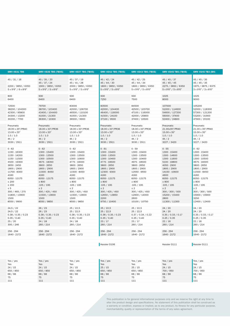
MODEL SMV 4127 TB5 SMV 4527 TB5 SMV 4527 TB6 SMV 4531 TB5 SMV 4531 TB6 SMV 4535 TB5 (TBX5) SMV 4537 TB5 (TBX5) SMV 4542 TB5 (TBX5) SMV 4543 TB5 (TBX5) SMV 4545 TB5 (TBX5) SMV 4545 TB3 (BH)

LIFT

ING

DAT

A

Dimensions Identifier UnitsLifting capacity at load center LC1 / LC2 / LC3 (no jacks) tons 41 / 27 / 14 45 / 27 / 14 45 / 27 / 14 45 / 31 / 16 45 / 31 / 16 45 / 35 / 20 45 / 37 / 19 45 / 42 / 24 45 / 42 / 25 45 / 45 / 37 45 / 45 / 35Lifting capacity at load center LC1 / LC2 / LC3 (with jacks) tons - - - - - 45 / 37 / 24 45 / 41 / 28 45 / 44 / 30 45 / 44 / 34 45 / 45 / 45 45 / 45 / 35Load centers in row 1 / 2 / 3 LC1 / LC2 / LC3 mm 2000 / 3850 / 6350 2000 / 3850 / 6350 2200 / 3850 / 6350 2000 / 3850 / 6350 2200 / 3850 / 6350 1900 / 3850 / 6350 2000 / 3850 / 6350 1800 / 3850 / 6350 1800 / 3850 / 6350 2275 / 3850 / 6350 1975 / 3875 / 6375Stacking height in row 1 (9'6" / 8'6") 5 x 9'6" / 5 x 8'6" 5 x 9'6" / 5 x 8'6" 5 x 9'6" / 6 x 8'6" 5 x 9'6" / 5 x 8'6" 5 x 9'6" / 6 x 8'6" 5 x 9'6" / 5 x 8'6" 5 x 9'6" / 5 x 8'6" 5 x 9'6" / 5 x 8'6" 5 x 9'6" / 5 x 8'6" 5 x 9'6" / 5 x 8'6" 3 x 9'6" / 3 x 8'6"Spreader type, telescopic, locking Toplift with 4 x twistlocks, extension 20-40 ft, 4 lifting eyes, safety locking (ELME 817) Lost load center to face of tires / jacks L4 mm 800 800 800 800 800 930 930 930 930 1025 1025Wheelbase L3 mm 6400 6400 6400 6400 6400 6400 6400 7250 7500 8000 9000

WEI

GH

T

Service weight kg 68500 68500 69200 71800 72500 79700 83000 83500 84500 107000 105200Axle pressure front LC1 (unloaded / rated load) kg 37500 / 96500 37500 / 102200 38200 / 104300 37500 / 102200 38200 / 104300 38700 / 103400 42000 / 106700 42000 / 104400 42500 / 103700 51000 / 114600 52000 / 118300Axle pressure rear LC1 (unloaded / rated load) kg 42000 / 88600 42000 / 88600 42300 / 88900 42000 / 95500 42300 / 95800 43400 / 104400 46500 / 110100 46400 / 116000 47100 / 116000 54600 / 127200 57300 / 121200Axle pressure front LC2 (unloaded / rated load) kg 31000 / 13000 31000 / 11300 31000 / 9900 34300 / 14600 34300 / 13200 41000 / 21300 41000 / 21300 41500 / 24100 42000 / 25800 56000 / 37400 53200 / 31900Axle pressure rear LC2 (unloaded / rated load) kg 26500 / 6900 26500 / 6900 26900 / 7300 29800 / 7300 30200 / 7700 36300 / 10300 36500 / 9900 37100 / 9500 37400 / 10500 52400 / 24800 47900 / 20100

WH

EELS

Tire type Pneumatic Pneumatic Pneumatic Pneumatic Pneumatic Pneumatic Pneumatic Pneumatic Pneumatic Pneumatic PneumaticInch 18.00 x 25"/PR40 18.00 x 25"/PR40 18.00 x 25"/PR40 18.00 x 25"/PR40 18.00 x 25"/PR40 18.00 x 33"/PR36 18.00 x 33"/PR36 18.00 x 33"/PR36 18.00 x 33"/PR36 21.00x35"/PR40 21.00 x 35"/PR40Inch 13.00 x 25" 13.00 x 25" 13.00 x 25" 13.00 x 25" 13.00 x 25" 13.00 x 33" 13.00 x 33" 13.00 x 33" 13.00 x 33" 15.00 x 35" 15.00 x 35"

Tire pressure, front / rear MPa 1.0 / 1.0 1.0 / 1.0 1.0 / 1.0 1.0 / 1.0 1.0 / 1.0 1.0 / 1.0 1.0 / 1.0 1.0 / 1.0 1.0 / 1.0 1.0 / 1.0 1.0 / 1.0Number of wheels, front / rear (X = driven) 4X / 2 4X / 2 4X / 2 4X / 2 4X / 2 4X / 2 4X / 2 4X / 2 4X / 2 4X / 2 4X / 2Track width, front / rear T1 / T2 mm 3030 / 2911 3030 / 2911 3030 / 2911 3030 / 2911 3030 / 2911 3030 / 2911 3030 / 2911 3030 / 2911 3030 / 2911 3227 / 3420 3227 / 3420

DIM

ENS

ION

S

Boom angle, min - max deg 0 - 62 0 - 62 0 - 62 0 - 62 0 - 62 0 - 62 0 - 62 0 - 61 0 - 59 0 - 55 0 - 62Lifting height in twistlocks, min - max at LC1 H1 - H2 mm 1150 - 15300 1150 - 15300 1150 - 15300 1150 - 15300 1150 - 16300 1300 - 15400 1300 - 15400 1300 - 15400 1300 - 15400 1300 - 15400 1300 - 15400Lifting height in twistlocks, min - max at LC2 H3 - H4 mm 1150 - 13400 1150 - 13400 1150 - 13400 1150 - 13400 1150 - 14200 1300 - 13500 1300 - 13500 1300 - 13500 1300 - 13500 1300 - 14600 1300 - 13500Lifting height in twistlocks, min - max at LC3 H5 - H6 mm 1150 - 10500 1150 - 10500 1150 - 10500 1150 - 10500 1150 - 11500 1300 - 10500 1300 - 10600 1300 - 10400 1300 - 10400 1300 - 11600 1300 - 10500Boom height, min - max H7 - H8 mm 4500 - 18200 4500 - 18200 4500 - 18200 4500 - 18200 4500 - 19300 4675 - 18350 4775 - 18400 4775 - 18500 4975 - 18500 5100 - 18800 4675 - 18300Truck height over cabin / seat height H9 - H10 mm 3650 - 2450 3650 - 2450 3650 - 2450 3650 - 2450 3650 - 2450 3800 - 2650 3800 - 2650 3800 - 2650 3800 - 2650 4050 - 2900 3800 - 2650Sliding cabin stroke (manual / hydraulic) L5 mm 1800 / 2900 1800 / 2900 1800 / 2900 1800 / 2900 1800 / 2900 1800 / 2900 1800 / 2900 1800 / 2900 1800 / 2900 1800 / 2900 1800 / 2900Overall length, with - without spreader L1 - L2 mm 11500 - 8300 11500 - 8300 11700 - 8300 11500 - 8300 11700 - 8300 11500 - 8450 11500 - 8450 12300 - 9300 12550 - 9550 14150 - 10600 11500 - 8450Drive axle width W1 mm 4160 4160 4160 4160 4160 4160 4160 4160 4160 4600 4160Spreader width, min - max W2 - W3 mm 6050 - 12175 6050 - 12175 6050 - 12175 6050 - 12175 6050 - 12175 6050 - 12175 6050 - 12175 6050 - 12175 6050 - 12175 6050 - 12175 6050 - 12175Spreader sideshift SS mm ± 800 ± 800 ± 800 ± 800 ± 200 ± 800 ± 800 ± 800 ± 800 ± 800 ± 800Spreader rotation SR deg -105 / 195 -105 / 195 -105 / 195 -105 / 195 ± 200 -105 / 195 -105 / 195 -105 / 195 -105 / 195 -105 / 195 -105 / 195Mechanical Pile Slope (side tilt / no power) PS deg ± 2 ± 2 ± 2 ± 2 ± 5 ± 2 ± 2 ± 2 ± 2 ± 2 ± 2Ground clearance, front / mid / steering axle C1 / C2 / C3 mm 300 / 465 / 275 300 / 465 / 275 300 / 465 / 275 300 / 465 / 275 300 / 465 / 275 300 / 425 / 450 300 / 425 / 450 300 / 425 / 450 300 / 425 / 450 300 / 300 / 500 300 / 300 / 500Aisle width (with 20 ft / 40 ft container) A1 / A2 mm 11500 / 13600 11500 / 13600 11800 / 13900 11500 / 13600 11800 / 13900 11500 / 13600 11500 / 13600 12650 / 13850 12900 / 14000 15200 / 15400 15900 / 15900Turning radius, inner R1 mm 1500 1500 1500 1500 1500 1500 1500 2200 2600 2800 3250Turning radius, outer 20 ft / outer 40 ft R2 / R3 mm 8550 / 9850 8550 / 9850 8550 / 9900 8550 / 9850 8550 / 9900 8550 / 9850 8550 / 9850 9750 / 10400 10100 / 10750 11300 / 11300 12400 / 12400

PER

FOR

MA

NC

E Drive speed forward, unloaded / at rated load km/h 25 / 22 25 / 22 25 / 22 24,5 / 22 24,5 / 22 26 / 23 25 / 22,5 25 / 22,5 25 / 22,5 24 / 20 24 / 20Drive speed reverse, unloaded / at rated load km/h 25 / 22 25 / 22 25 / 22 24,5 / 22 24,5 / 22 26 / 23 25 / 22,5 25 / 22,5 25 / 22,5 24 / 20 24 / 20Lifting speed, unloaded / at 40% load / at rated load m/s 0.38 / 0.35 / 0.23 0.38 / 0.35 / 0.23 0.38 / 0.35 / 0.23 0.38 / 0.35 / 0.23 0.38 / 0.35 / 0.23 0.38 / 0.35 / 0.23 0.38 / 0.35 / 0.23 0.38 / 0.35 / 0.23 0.37 / 0.34 / 0.22 0.35 / 0.33 / 0.17 0.35 / 0.33 / 0.17Lowering speed, unloaded / at rated load m/s 0.35 / 0.40 0.35 / 0.40 0.35 / 0.40 0.35 / 0.40 0.35 / 0.40 0.35 / 0.40 0.35 / 0.40 0.35 / 0.40 0.35 / 0.40 0.25 / 0.35 0.25 / 0.35Gradeability, at rated load, 0/2 km/h % / % 29 / 22 29 / 22 25 / 20 25 / 20 25 / 20 24 / 18 24 / 18 23 / 17 23 / 17 22 / 16 22 / 16Towing power, at rated load, 0/2 km/h kN / kN 315 / 251 315 / 251 300 / 246 300 / 246 300 / 246 260 / 214 260 / 214 260 / 214 260 / 214 260 / 214 260 / 214

DR

IVEL

INE

Engine power (min - max) EU2 / EU3b kW 256 - 294 256 - 294 256 - 294 256 - 294 256 - 294 256 - 294 256 - 294 256 - 294 256 - 294 256 - 294 256 - 294Engine torque (min - max) EU2 / EU3b Nm 1640 - 2172 1640 - 2172 1640 - 2172 1640 - 2172 1640 - 2172 1640 - 2172 1640 - 2172 1640 - 2172 1640 - 2172 1640 - 2172 1640 - 2172Transmission, gears forward + reverse DANA 4 + 4 / ZF 4 + 3Transmission type, function, shifting Automatic transmission, torque converter, reverse protection, powershiftDrive axle model Kessler D102 Kessler D106 Kessler D111 Kessler D111Driving brake system, type Oil-cooled multiple wet disc brakes (WDB)Parking brake system, type Dry single disc / spring releaseSteering system / steering axle type Hydraulic power steer / HD axle + double-acting cylinder

OTH

ERS

Load-sensing hydraulics / power-on-demand Yes / yes Yes / yes Yes / yes Yes / yes Yes / yes Yes / yes Yes / yes Yes / yes Yes / yes Yes / yes Yes / yesYes Yes Yes Yes Yes Yes Yes Yes Yes Yes Yes

Hydraulic oil pressure, boom / spreader MPa 24 / 15 24 / 15 24 / 15 24 / 15 24 / 15 24 / 15 24 / 15 25 / 15 25 / 15 24 / 15 24 / 15Diesel / hydraulic tank volumes Lit 650 / 850 650 / 850 650 / 850 650 / 850 650 / 850 650 / 850 650 / 850 650 / 850 650 / 850 700 / 950 700 / 950Noise level inside cab (LM) DIN 45635 EU2 / EU3b dB(A) 68 / 66 68 / 66 68 / 66 68 / 66 68 / 66 68 / 66 68 / 66 68 / 66 68 / 66 68 / 66 68 / 66Noise level inside cab (LpAZ) EN 12053 dB(A) 75 75 75 75 75 75 75 75 75 75 75Noise level outside (LWA) 2000/14/EC dB(A) 111 111 111 111 111 111 111 111 111 111 111

NOTE 1. TB models do not have support jacks / TBX models have support jacks for increased capacity and lower ground pressureNOTE 2. Other lifting attachment combinations possible, check factory informationNOTE 3. Four lifting eyes on spreader are standard; extra ones can be provided plus container guides on one side of spreaderNOTE 4. Optional for laden handlers: Hydraulic Pile Slope ±6 deg and Powered Dampening Cylinders ±5 deg + tilt lockNOTE 5. For available driveline combinations, see driveline chart and latest factory informationNOTE 6. BH = reach stacker for barge handling (other models available)

This publication is for general informational purposes only and we reserve the right at any time to alter the product design and specifications. No statement of this publication shall be construed as a warranty or condition, express or implied, as to any product, its fitness for any particular purpose, merchantability, quality or representation of the terms of any sales agreement.

B.2 Elme, Model 817

This section is a brochure from ELME about their product Model 8172 which is aspreader used on reach stackers.

2Elme. MODEL 817. Last visited 17 September 2016. URL: http://www.elme.com/wp-content/blogs.dir/1/files_mf/1446562773ELMELeaflet_Model817.pdf

54

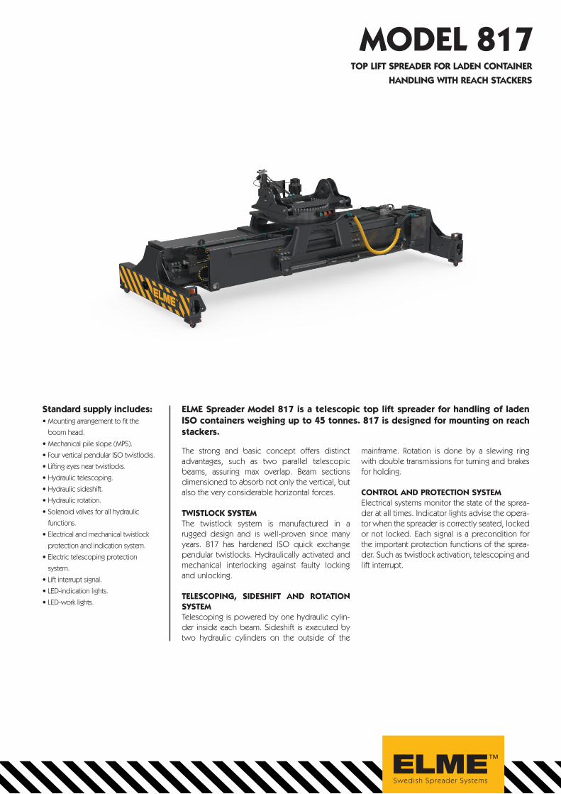
MODEL 817

ELME Spreader Model 817 is a telescopic top lift spreader for handling of laden ISO containers weighing up to 45 tonnes. 817 is designed for mounting on reach stackers.

The strong and basic concept offers distinct advantages, such as two parallel telescopic beams, assuring max overlap. Beam sections dimensioned to absorb not only the vertical, but also the very considerable horizontal forces. TWISTLOCK SYSTEMThe twistlock system is manufactured in a rugged design and is well-proven since many years. 817 has hardened ISO quick exchange pendular twistlocks. Hydraulically activated and mechanical interlocking against faulty locking and unlocking.

TELESCOPING, SIDESHIFT AND ROTATION SYSTEMTelescoping is powered by one hydraulic cylin-der inside each beam. Sideshift is executed by two hydraulic cylinders on the outside of the

mainframe. Rotation is done by a slewing ring with double transmissions for turning and brakes for holding.

CONTROL AND PROTECTION SYSTEMElectrical systems monitor the state of the sprea-der at all times. Indicator lights advise the opera-tor when the spreader is correctly seated, locked or not locked. Each signal is a precondition for the important protection functions of the sprea-der. Such as twistlock activation, telescoping and lift interrupt.

TOP LIFT SPREADER FOR LADEN CONTAINER HANDLING WITH REACH STACKERS

Standard supply includes:• Mounting arrangement to fit the boom head.• Mechanical pile slope (MPS). • Four vertical pendular ISO twistlocks. • Lifting eyes near twistlocks.• Hydraulic telescoping.• Hydraulic sideshift.• Hydraulic rotation. • Solenoid valves for all hydraulic functions.• Electrical and mechanical twistlock protection and indication system.• Electric telescoping protection system.• Lift interrupt signal. • LED-indication lights.• LED-work lights.

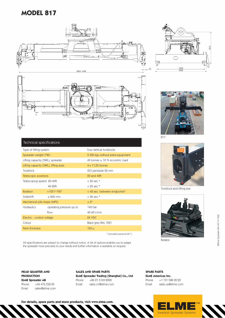
MODEL 817

©El

me

Spre

ader

AB

• 81

7 •

1506

Type of lifting system Four vertical twistlocks

Spreader weight (TW) 9 300 kgs without extra equipment

Lifting capacity (SWL), spreader 45 tonnes ± 10 % eccentric load

Lifting capacity (SWL), lifting eyes 4 x 11,25 tonnes

Twistlock ISO pendular 20 mm

Telescopic positions 20 and 40ft

Telescoping speed 20-40ft < 20 sec.*

40-20ft < 25 sec.*

Rotation +105°/-195° < 42 sec. between endpoints*

Sideshift ± 800 mm < 26 sec.*

Mechanical pile slope (MPS) ± 2°

Hydraulics operating pressure up to 140 bar

flow 40-60 L/min

Electric - control voltage 24 VDC

Colour Black grey RAL 7021

Paint thickness 150 µ

All specifications are subject to change without notice. A list of options enables you to adaptthe spreader more precisely to your needs and further information is available on request.

817.

Twistlock and lifting eye.

Rotator.

* Calculated speed at 20° C.

HEAD QUARTER AND PRODUCTIONELME Spreader ABPhone +46 476 558 00Email sales@elme.com

SALES AND SPARE PARTSELME Spreader Trading (Shanghai) Co., LtdPhone +86 21 5169 8922Email sales.cn@elme.com

SPARE PARTSELME Americas Inc.Phone +1 731 588 02 20Email sales.us@elme.com

For details, spare parts and more products, visit www.elme.com.

Technical specifications