Real-Time Lime Quality Control through Process Automation

International Journal of Emerging Science and Engineering (IJESE) ISSN: 2319–6378 (Online), Volume-7 Issue-2, May 2021

1

Published By: Blue Eyes Intelligence Engineering and Sciences Publication © Copyright: All rights reserved.

Retrieval Number: 100.1/ijese.B2502057221 DOI: 10.35940/ijese.B2502.057221 Journal Website: www.ijese.org

Real-Time Lime Quality Control through Process Automation

Vipul Kumar Tiwari, Abhishek Choudhary, Umesh Kr. Singh, Anil Kumar Kothari, Manish Kr. Singh

Abstract: In the steel industry - Tata steel, India, most of the lime produced in the lime plant is used in the steel-making pro-cess at LD shops. The quality of steel produced at LD shops de-pends on the quality of lime used. Moreover, the lime also helps in the crucial dephosphorization process during steel-making. The calcined lime produced in the lime plant goes to the labora-tory for testing its final quality (CaO%), which is very difficult to control. To predict, control and enhance the quality of lime dur-ing lime making process, five machine-learning-based models such as multivariate linear regression, support vector machine, decision tree, random forest and extreme gradient boosting have been developed using different algorithms. Python has been used as a tool to integrate the algorithms in the models. Each model has been trained on the past 14 months’ data of process parame-

ters, collected from level 1 sensor devices, to predict the future quality of lime. To boost the model’s prediction performance,

hyper-parameter tuning has been performed using grid-search algorithm. A comparative study has been done among all the models to select a final model with the least root mean square error in predicting and control future lime quality. After the comparison, results show that the model incorporating support vector machine algorithm has least value of root mean square error of 1.23 in predicting future lime quality. In addition to this, a self-learning approach has also been incorporated into support vector machine model to enhance its performance further in real-time. The result shows that the performance has been boosted from 85% strike-rate in +/-2 error range to 90% of strike-rate in +/-1 error range in real-time. Further, the above predictive model has been extended to build a control model which gives prescrip-tions as output to control the future quality of lime. For this pur-pose, a golden batch of good data has been fetched which has shown the best quality of lime (≥ 94% of CaO%). A good range of process parameters has been extracted in the form of upper control limit and lower control limit to tune the set-points and to give the prescriptions to the user. The integration of these two models (Predictive model and control model) helps in controlling the quality of lime 12 hours before its final production of lime in lime plant. Results show that both models (Predictive model and control model) have 90% of strike-rate within +/-1 of error in real-time. Finally, a human machine interface has been devel-oped to facilitate the user to take action based on control model’s

output. Eventually this work is deployed as a lime making process automation to predict and control the lime quality.

Keywords: Steel-Making, Quality Control, Process Automa-tion, Machine-Learning, Human-Machine-Interface. Manuscript received on May 03, 2021. Revised Manuscript received on May 08, 2021. Manuscript published on May 30, 2021. * Correspondence Author

Vipul Kumar Tiwari*, Technologist, Automation Division, Tata Steel, Jamshedpur, 831001, India. E-mail: [email protected]

Abhishek Choudhary, Sr. Manager, Lime plant, Tata Steel, Jamshed-pur, 831001, India. E-mail: abhishek.c@ tatasteel.com

Umesh Kr. Singh, Principal Technologist, Automation Division, Tata Steel, Jamshedpur, 831001, India. E-mail: [email protected]

Anil Kumar Kothari, Chief (SM&C), Automation Division, Tata Steel, Jamshedpur, 831001, India. E-mail: [email protected]

Manish Kr. Singh, Chief (One IT), Automation Division, Tata Steel, Jamshedpur, 831001, India. E-mail: [email protected] © The Authors. Published by Blue Eyes Intelligence Engineering and Sci-ences Publication (BEIESP). This is an open access article under the CC BY-NC-ND license (http://creativecommons.org/licenses/by-nc-nd/4.0/)

I. INTRODUCTION

The world production of lime is estimated around 350 million tons and 40-45% of lime is used in steel manufactur-ing industry globally [1]. Lime as a basic flux plays an im-portant role in the mechanism of metallurgical reactions in steel-making processes [2]. Addition of lime in steel-making, as shown in Fig. 1, controls the removal of sulphur, which is an unwanted impurity [3]. It is also a critical addi-tive used to form a quality sinter, which is used in iron-making process [4]. Eventually, lime quality has a signifi-cant impact on steel quality, its metallurgical properties, productivity and total cost of production [1].

Fig. 1. Lime used in the steel making process.

In lime plant of Tata Steel, this crucial flux lime (CaO),

an oxide of calcium, is produced from the limestone (Ca-CO3) in the presence of a heating agent through below cal-cination reaction as shown in (1).

CaCO3 CaO + CO2

(1)

To complete the above thermal decomposition of lime-

stone into lime, the stones must be heated to the dissociation temperature of the carbonates [5]. The above reaction occurs in a Merz-kiln shaft which takes limestone along with com-bustion gases as input and produces lime as a product (see Fig. 2).

heat

https://www.openaccess.nl/en/open-publications

http://www.ijese.org/

mailto:[email protected]

mailto:abhishek.c@%20tatasteel.com




http://creativecommons.org/licenses/by-nc-nd/4.0/

https://crossmark.crossref.org/dialog/?doi=10.35940/ijese.B2502.057221&domain=www.ijese.org


2



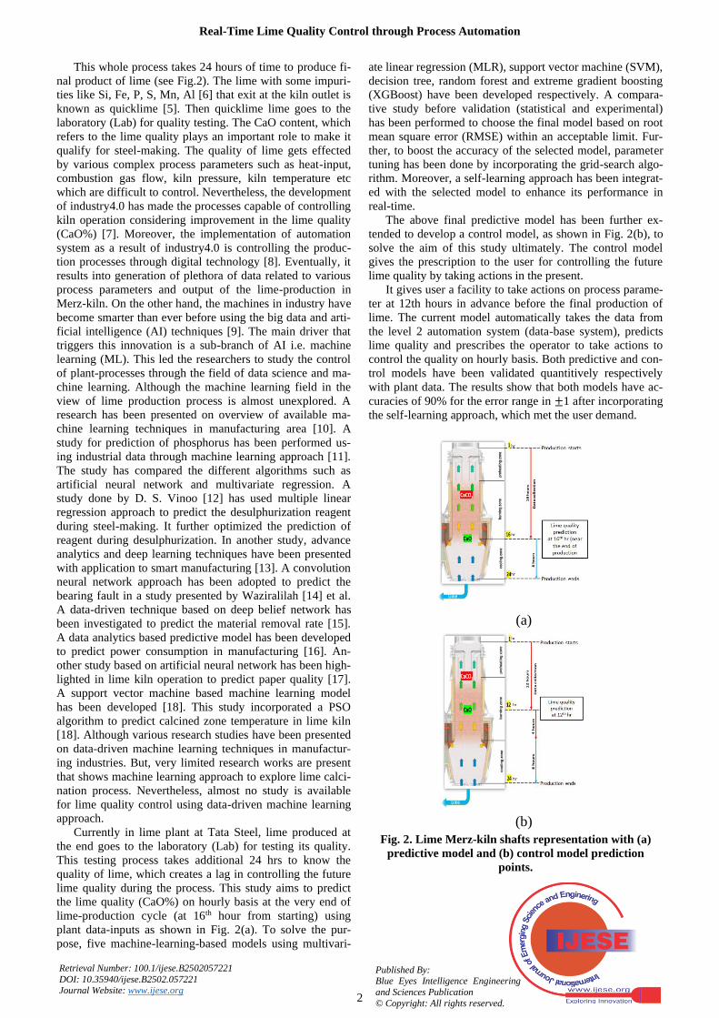
This whole process takes 24 hours of time to produce fi-nal product of lime (see Fig.2). The lime with some impuri-ties like Si, Fe, P, S, Mn, Al [6] that exit at the kiln outlet is known as quicklime [5]. Then quicklime lime goes to the laboratory (Lab) for quality testing. The CaO content, which refers to the lime quality plays an important role to make it qualify for steel-making. The quality of lime gets effected by various complex process parameters such as heat-input, combustion gas flow, kiln pressure, kiln temperature etc which are difficult to control. Nevertheless, the development of industry4.0 has made the processes capable of controlling kiln operation considering improvement in the lime quality (CaO%) [7]. Moreover, the implementation of automation system as a result of industry4.0 is controlling the produc-tion processes through digital technology [8]. Eventually, it results into generation of plethora of data related to various process parameters and output of the lime-production in Merz-kiln. On the other hand, the machines in industry have become smarter than ever before using the big data and arti-ficial intelligence (AI) techniques [9]. The main driver that triggers this innovation is a sub-branch of AI i.e. machine learning (ML). This led the researchers to study the control of plant-processes through the field of data science and ma-chine learning. Although the machine learning field in the view of lime production process is almost unexplored. A research has been presented on overview of available ma-chine learning techniques in manufacturing area [10]. A study for prediction of phosphorus has been performed us-ing industrial data through machine learning approach [11]. The study has compared the different algorithms such as artificial neural network and multivariate regression. A study done by D. S. Vinoo [12] has used multiple linear regression approach to predict the desulphurization reagent during steel-making. It further optimized the prediction of reagent during desulphurization. In another study, advance analytics and deep learning techniques have been presented with application to smart manufacturing [13]. A convolution neural network approach has been adopted to predict the bearing fault in a study presented by Waziralilah [14] et al. A data-driven technique based on deep belief network has been investigated to predict the material removal rate [15]. A data analytics based predictive model has been developed to predict power consumption in manufacturing [16]. An-other study based on artificial neural network has been high-lighted in lime kiln operation to predict paper quality [17]. A support vector machine based machine learning model has been developed [18]. This study incorporated a PSO algorithm to predict calcined zone temperature in lime kiln [18]. Although various research studies have been presented on data-driven machine learning techniques in manufactur-ing industries. But, very limited research works are present that shows machine learning approach to explore lime calci-nation process. Nevertheless, almost no study is available for lime quality control using data-driven machine learning approach.

Currently in lime plant at Tata Steel, lime produced at the end goes to the laboratory (Lab) for testing its quality. This testing process takes additional 24 hrs to know the quality of lime, which creates a lag in controlling the future lime quality during the process. This study aims to predict the lime quality (CaO%) on hourly basis at the very end of lime-production cycle (at 16th hour from starting) using plant data-inputs as shown in Fig. 2(a). To solve the pur-pose, five machine-learning-based models using multivari-

ate linear regression (MLR), support vector machine (SVM), decision tree, random forest and extreme gradient boosting (XGBoost) have been developed respectively. A compara-tive study before validation (statistical and experimental) has been performed to choose the final model based on root mean square error (RMSE) within an acceptable limit. Fur-ther, to boost the accuracy of the selected model, parameter tuning has been done by incorporating the grid-search algo-rithm. Moreover, a self-learning approach has been integrat-ed with the selected model to enhance its performance in real-time.

The above final predictive model has been further ex-tended to develop a control model, as shown in Fig. 2(b), to solve the aim of this study ultimately. The control model gives the prescription to the user for controlling the future lime quality by taking actions in the present.

It gives user a facility to take actions on process parame-ter at 12th hours in advance before the final production of lime. The current model automatically takes the data from the level 2 automation system (data-base system), predicts lime quality and prescribes the operator to take actions to control the quality on hourly basis. Both predictive and con-trol models have been validated quantitively respectively with plant data. The results show that both models have ac-curacies of 90% for the error range in ±1 after incorporating the self-learning approach, which met the user demand.

Fig. 2. Lime Merz-kiln shafts representation with (a) predictive model and (b) control model prediction

points.

(a)

(b)



3



II. METHODOLOGY

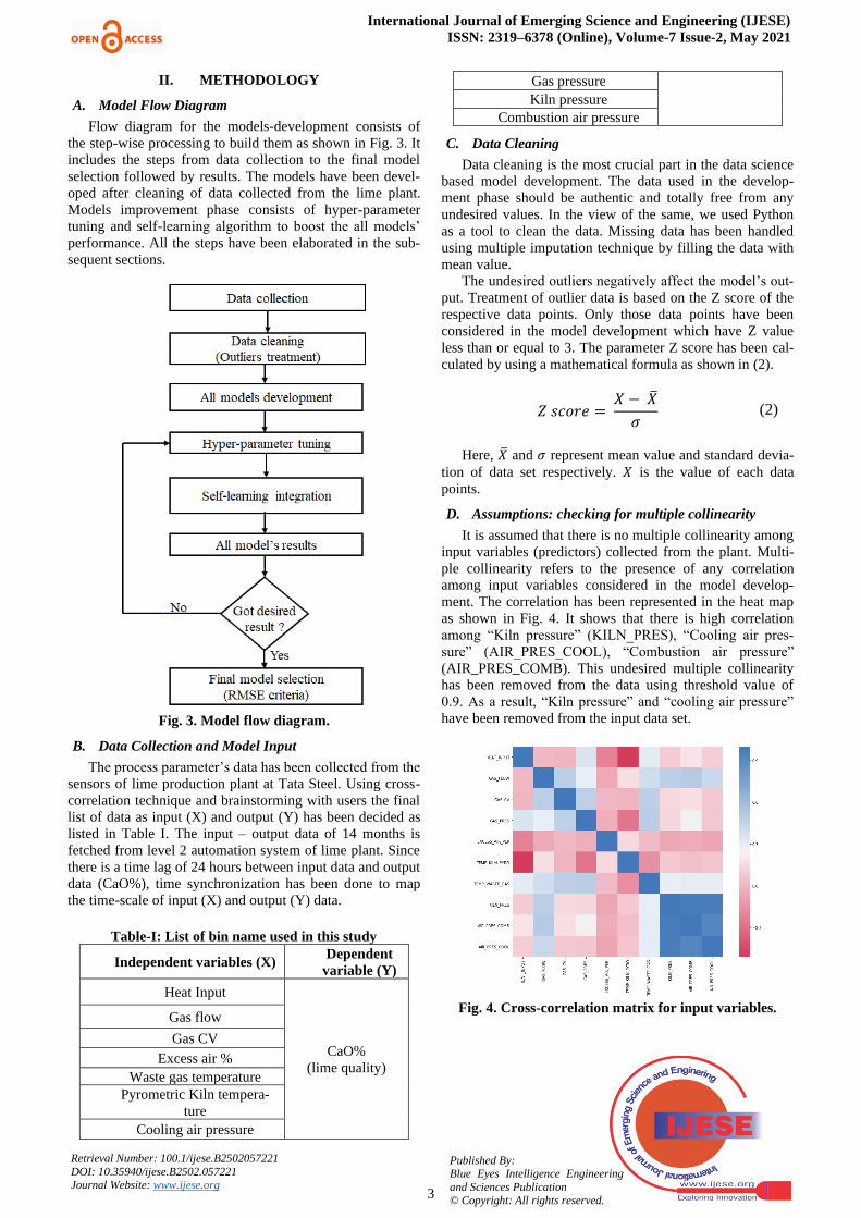
A. Model Flow Diagram

Flow diagram for the models-development consists of the step-wise processing to build them as shown in Fig. 3. It includes the steps from data collection to the final model selection followed by results. The models have been devel-oped after cleaning of data collected from the lime plant. Models improvement phase consists of hyper-parameter tuning and self-learning algorithm to boost the all models’

performance. All the steps have been elaborated in the sub-sequent sections.

Fig. 3. Model flow diagram.

B. Data Collection and Model Input

The process parameter’s data has been collected from the

sensors of lime production plant at Tata Steel. Using cross-correlation technique and brainstorming with users the final list of data as input (X) and output (Y) has been decided as listed in Table I. The input – output data of 14 months is fetched from level 2 automation system of lime plant. Since there is a time lag of 24 hours between input data and output data (CaO%), time synchronization has been done to map the time-scale of input (X) and output (Y) data.

Table-I: List of bin name used in this study

Independent variables (X) Dependent

variable (Y)

Heat Input

CaO% (lime quality)

Gas flow

Gas CV Excess air %

Waste gas temperature Pyrometric Kiln tempera-

ture Cooling air pressure

Gas pressure Kiln pressure

Combustion air pressure

C. Data Cleaning

Data cleaning is the most crucial part in the data science based model development. The data used in the develop-ment phase should be authentic and totally free from any undesired values. In the view of the same, we used Python as a tool to clean the data. Missing data has been handled using multiple imputation technique by filling the data with mean value.

The undesired outliers negatively affect the model’s out-

put. Treatment of outlier data is based on the Z score of the respective data points. Only those data points have been considered in the model development which have Z value less than or equal to 3. The parameter Z score has been cal-culated by using a mathematical formula as shown in (2).

𝑍 𝑠𝑐𝑜𝑟𝑒 = 𝑋 −

𝜎 (2)

Here, and 𝜎 represent mean value and standard devia-

tion of data set respectively. 𝑋 is the value of each data points.

D. Assumptions: checking for multiple collinearity

It is assumed that there is no multiple collinearity among input variables (predictors) collected from the plant. Multi-ple collinearity refers to the presence of any correlation among input variables considered in the model develop-ment. The correlation has been represented in the heat map as shown in Fig. 4. It shows that there is high correlation among “Kiln pressure” (KILN_PRES), “Cooling air pres-

sure” (AIR_PRES_COOL), “Combustion air pressure”

(AIR_PRES_COMB). This undesired multiple collinearity has been removed from the data using threshold value of 0.9. As a result, “Kiln pressure” and “cooling air pressure”

have been removed from the input data set.

Fig. 4. Cross-correlation matrix for input variables.




4



III. MODEL DEVELOPMENT

Python as a tool has been used to develop the model for this work. In this study, following five predictive models have been developed and the best model has been chosen based on root mean square error (RSME).

A. Multivariate Linear Regression

Multivariate linear regression is one of the basic tech-nique which gives the relationship between features (inde-pendent variables) and predicted variable (dependent pa-rameter).

Equation (4) shows mathematical expression for simple linear regression where only two independent variables are present but in multiple linear regression there are more than two independent variables as shown in (5) [19].

𝑌 = 𝐴𝑋 + 𝐵 (4)

𝑌𝑖 = 𝛽0 + 𝛽1𝑋𝑖1+ 𝛽2𝑋𝑖2

… … … … … + 𝛽𝑛𝑋𝑖𝑛 (5)

Here, 𝑌 = Dependent parameter (Output), 𝑋 = Independ-

ent parameter (Input) and 𝐴, 𝐵 and 𝛽 are regression parame-ters.

B. Support Vector Machine

The basic concept behind support vector machine (SVM) is to map the original data 𝑋 into feature space as function 𝐹(𝑋) with higher dimensionality through a non-linear map-ping function and construct an optimal hyperplane in a new space [20]. This non-linear function 𝐹(𝑋) is defined such that it minimizes the loss function 𝑙𝜀 as shown in (6) and (7) respectively [21].

𝐹(𝑋) = ∑(𝛼𝑖∗ − 𝛼𝑖)𝐾(𝑋, 𝑋𝑖

𝑁

𝑖=1

) + 𝐵 (6)

Here, (𝛼𝑖

∗, 𝛼𝑖 > 0), 𝐵, 𝐾 are Lagrange multipliers, bias term and kernel function respectively [20]. 𝑋, 𝑋𝑖 are the in-dependent variable’s data points.

𝑙𝜀(𝑦𝑖 − 𝐹(𝑋𝑖)) = 0 𝑓𝑜𝑟 |𝑦𝑖 − 𝐹(𝑋𝑖)| < 𝜀

= |𝑦𝑖 − 𝐹(𝑋𝑖)| for other cases (7)

Here, yi is target (dependent) variables and ε is the dif-

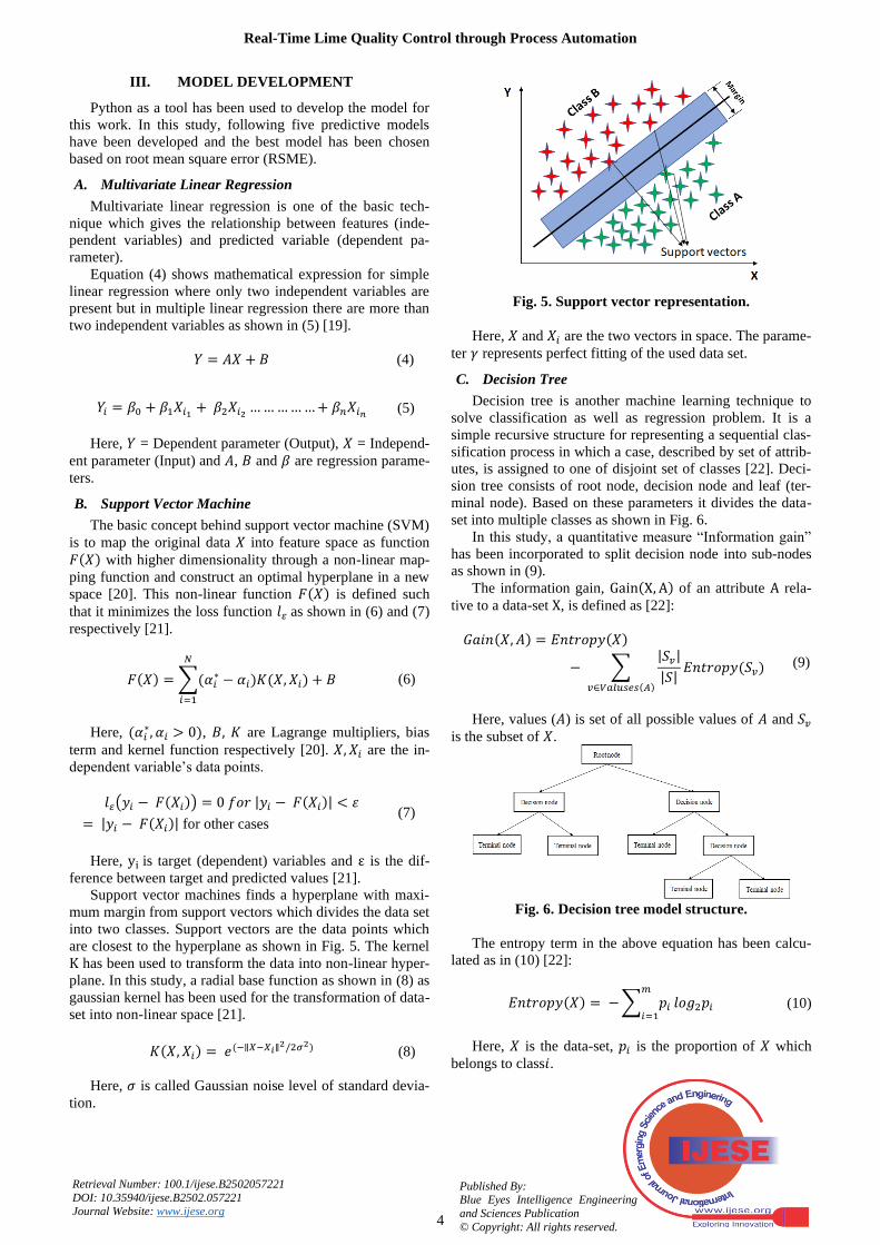
ference between target and predicted values [21]. Support vector machines finds a hyperplane with maxi-

mum margin from support vectors which divides the data set into two classes. Support vectors are the data points which are closest to the hyperplane as shown in Fig. 5. The kernel K has been used to transform the data into non-linear hyper-plane. In this study, a radial base function as shown in (8) as gaussian kernel has been used for the transformation of data-set into non-linear space [21].

𝐾(𝑋, 𝑋𝑖) = 𝑒(−∥𝑋−𝑋𝑖∥2/2𝜎2) (8)

Here, 𝜎 is called Gaussian noise level of standard devia-

tion.

Fig. 5. Support vector representation.

Here, 𝑋 and 𝑋𝑖 are the two vectors in space. The parame-

ter 𝛾 represents perfect fitting of the used data set.

C. Decision Tree

Decision tree is another machine learning technique to solve classification as well as regression problem. It is a simple recursive structure for representing a sequential clas-sification process in which a case, described by set of attrib-utes, is assigned to one of disjoint set of classes [22]. Deci-sion tree consists of root node, decision node and leaf (ter-minal node). Based on these parameters it divides the data-set into multiple classes as shown in Fig. 6.

In this study, a quantitative measure “Information gain”

has been incorporated to split decision node into sub-nodes as shown in (9).

The information gain, Gain(X, A) of an attribute A rela-tive to a data-set X, is defined as [22]:

𝐺𝑎𝑖𝑛(𝑋, 𝐴) = 𝐸𝑛𝑡𝑟𝑜𝑝𝑦(𝑋)

− ∑|𝑆𝑣|

|𝑆|𝑣∈𝑉𝑎𝑙𝑢𝑠𝑒𝑠(𝐴)

𝐸𝑛𝑡𝑟𝑜𝑝𝑦(𝑆𝑣) (9)

Here, values (𝐴) is set of all possible values of 𝐴 and 𝑆𝑣

is the subset of 𝑋.

Fig. 6. Decision tree model structure.

The entropy term in the above equation has been calcu-

lated as in (10) [22]:

𝐸𝑛𝑡𝑟𝑜𝑝𝑦(𝑋) = − ∑ 𝑝𝑖

𝑚

𝑖=1𝑙𝑜𝑔2𝑝𝑖 (10)

Here, 𝑋 is the data-set, 𝑝𝑖 is the proportion of 𝑋 which

belongs to class𝑖.



5



D. Random Forest

Random forest, another supervised regression technique, is an extension of above decision tree algorithm explained previously. It divides the whole data-set into number of sub-sets which are used to form the multiple regression trees [23] as shown in Fig. 7. Further it combines all the modelled trees and forms the best model. Random forest algorithm uses bootstrap sampling for sampling of input data [23].

Fig. 7. Random forest multiple trees structure.

E. Extreme Gradient Boosting (XGBoost)

It is another tree based supervised machine learning al-gorithm. It is an efficient and scalable implementation of gradient boosting algorithm [24]. To formulate the model, an objective function 𝐹𝑜𝑏𝑗 is defined in (11) which compris-es of an error term (L) and regularization term (Ω) [25].

𝐹𝑜𝑏𝑗(∅) = 𝐿(∅) + Ω(∅) (11)

Here,

𝐿(∅) = 𝑙(𝑦, 𝑦𝑝) + 𝛼𝑇 (12)

Ω(∅) =1

2(𝛾 ∥ 𝑤 ∥2)

(13)

The terms 𝑙, 𝑦, 𝑦𝑝, 𝛼, 𝑇, 𝛾 and 𝑤 in the above (12) and

(13) represents loss function, target value (output), predicted value, learning rate, number of leaf in the tree, regulariza-tion parameter and weight of the leaf respectively [23]. The loss function expressed in above (12) is mathematically de-fined in the forms of mean square error as shown in (14).

𝑙(𝑦, 𝑦𝑝) = (𝑦 − 𝑦𝑝)2 (14)

The objective function 𝐹𝑜𝑏𝑗 is minimized considering

optimization of its weightage parameters.

IV. FINAL MODEL SELECTION AND PERFOR-MANCE BOOSTING

All the models have been implemented through cross validation technique [26]. Whole data (feature variables and target variable) was bifurcated into training data and test data for cross-validation of regression models as shown in Fig. 8. At first stage, the models have been trained on train-ing data-set and then it is fitted to the test data set. In this work, 80% of the data has been chosen for training and 20% of the data has been used for testing.

Fig. 8. Cross-validation of the model.

A. Final Model Selection

Considering the goal of this study, all model’s perfor-

mances have been evaluated on the basis of root mean square error (RMSE). The two performance evaluation met-rics are given by the below mathematical (15) and (16). The final model has been selected which has the least RMSE [29].

n

XXRMSE

n

i imio =−

= 1

2,, )(

(15)

There is another evaluation parameter called mean abso-

lute error (MAE) as shown in (18).

=MAEn

XXn

i imio =−

1 ,, )( (16)

Where Xo represents observed values and Xm is modelled

values at ith time.

B. Performance Boosting

Below are the two measures which have been incorpo-rated to improve the models’ performance:

(a) Hyper-Parameter Tuning

Hyper-parameters incorporated in the all machine learn-ing kernels play a crucial role in transforming the data from linear to non-linear space. The different hyper-parameters used in the model have been tuned in iterations using the grid-search algorithm [27, 28]. The grid-search algorithm optimizes the models’ hyper-parameters using the above cross-validation technique as shown in Fig. 9.




6



Fig. 9. Grid-search algorithm in SVM model.

In this study, hyper-parameters of all the above models

have been optimized. One of the models, i.e. SVM model, gave the best accuracy in output with optimized hyper-parameters with C (regularization parameter), 𝛾 (gamma) and 𝜀 (loss function) having values 0.005, 0.5 and 0.0001 respectively.

(b) Self-learning Algorithm

In this study, a self-learning algorithm has been incorpo-rated based on exponential time-series technique at the stage of implementation of the SVM model in the real-time. This integration of self-learning approach in the final model cor-rects the real-time error and improves the hourly predictions of lime quality (CaO %) as expressed in (18). A correction factor (𝐶𝑓) based on exponential time-series technique has been calculated as shown in (17).

𝐶𝑓 = 𝑤1(𝐶𝑎 − 𝐶𝑝) + 𝑤2(𝐶𝑎 − 𝐶𝑝) … … …

+ 𝑤𝑛(𝐶𝑎 − 𝐶𝑝)

(17)

Here, 𝐶𝑎 = Actual CaO %

𝐶𝑝 = Predicted CaO %

𝑤𝑛 is the correction coefficient where 𝑊1 > 𝑊2 >…….> 𝑊𝑛

Hence final prediction equation is given as:

𝐶𝑝𝑡′ = 𝐶𝑝𝑡

+ 𝐶𝑓 (18) Where 𝐶𝑝𝑡

′ 𝑎𝑛𝑑 𝐶𝑝𝑡 is predicted CaO% and corrected

prediction at time t respectively.

V. CONTROL MODEL DEVELOPMENT

Based on the CaO% prediction of above predictive mod-el with least RSME, a control model has been developed. The golden batch of input data that resulted into acceptable quality of lime (CaO%) has been used to calculate lower control limit (LCL) and upper control limit (UCL) for the

variation of process parameters. It checks for any abnormal variation in process parameter values based LCL and UCL. Finally, it gives the action points as prescription to tune the process parameters’ s value for controlling the future lime

quality (CaO%) 12 hours before the final production of lime. Therefore, user gets enough time to control the lime quality during the production and eventually 24 hours’ time

lag is eliminated. Fig. 10 shows the control model working to tune the set points on hourly basis.

Fig. 10. Working of control model.

VI. RESULTS AND VALIDATION

This section includes the all results obtained and their visualization from the best model, i.e. SVM. The results have been validated with experimental data of the corre-sponding kiln. At first, the best model has been chosen using performance metric and then CaO% prediction results have been presented and validated for that model. Moreover, val-idation of prescriptive model result with experimental data has also been included followed by prediction.

A. Model Performance Evaluation Metric

The different metrics listed in Table II are used for measuring the model’s performance through comparison.

Table-II: Models metrics.

Model names Mean absolute error (MAE)

Root mean square error (RMSE)

Multivariate linear regression

0.96 1.26

Support vector machine

0.92 1.23

Decision tree 0.92 1.26 Radom forest 1.02 1.31

Extreme gradient boosting

1.10 1.46

From the above values of RMSE, it is clear that support

vector machine model (SVM) has the least value of error among all. The value RMSE of magnitude 1.23 is found acceptable as per user demand. Eventually, SVM model has been chosen as the best model for this study.



7



B. Feature Importance

Below Fig. 11 shows the importance of the features (in-put parameters) in predicting the final output (CaO%) based on standardized coefficients of all process parameters. Fea-ture importance helps in knowing the importance of process parameters in predicting the lime quality.

Fig. 11. Feature importance of input parameters.

C. Visualization of Actual CaO% and Predicted CaO%

Below Fig. 12 shows the variation of actual CaO% and predicted CaO% during the prediction cycle. It is observed that model has captured enough variation of actual CaO% in predicting the future value of CaO%.

Fig. 12. Line plot of actual CaO% and predicted CaO%.

D. Variation within Residuals

Variation of residuals (deviation of predicted CaO% from actual CaO%) has been shown in the below Fig. 13 as box plot. Since the median value of the residual is near zero, it is concluded that 75% of the residual fall between the rage of -1 and 1.

Fig. 13. Box plot of residuals.

E. Model Validation Test

A validation test has also been performed based on qualitative and quantitative parameters respectively. Model

has been validated with real time plant data (experimental data) of CaO%.

(a) Validation with real-time experimental data

In this study, the predictive model performance has also been validated with the real-time experimental data (Lab data) of CaO%. For this purpose, the model was deployed in the real-time production and a quantitative study has been performed to test the validity of prediction of CaO% with experimental result (lab data). Moreover, the same valida-tion study has also been performed for prescriptive model.

(a.1) Predictive Model Validation In Real-Time

Validation of predictive model with real-time experi-mental data (Lab data) has been presented in Fig. 14. It is observed from the plot that model has very close prediction of CaO% with actual experimental data. Quantitatively, the model has given the accuracy of 90% in error range of -1 to 1 with integration of self-learning approach.

(a.1.1) Validation of predicted CaO% with actual CaO%

Figure 14 shows the comparison graph for actual CaO% (plant data) and predicted CaO% when prediction cycle was run hourly in real-time. Fig. 15 shows the frequency of error came between the range of -1 and 1 while testing the model on 187 data points. It is clear that more than 90% of the er-ror fell into the band of -1 and 1.

Fig. 14.Variation of actual and predicted CaO%.

Fig. 15. Strike-rate visualization of predictive model.

0.20.14

0.130.13

0.120.12

0.10.06

0 0.05 0.1 0.15 0.2 0.25

GAS_FLOW

GAS_PRES

GAS_CV

TEMP_KILN_PYRO

Feature importance

Par

amet

ers

85

90

95

100

1 9 17 25 33 41 49 57 65 73 81 89 97 105

113

121

129

137

145

153

CaO

%

Time (hr)

Actual CaO% and Predicted CaO%

Y_Predicted Y_Actual

90

91

92

93

94

95

96

1 11 21 31 41 51 61 71 81 91 101

111

121

131

141

151

161

171

181

CaO

%

Time (hr)

Actual CaO% and predicted CaO%

PRED_CAO ACT_CAO




8



(a.1.2) Variation of residual during prediction

Below Fig. 16 shows the variation of residual error (De-viation of predicted CaO% from actual CaO%) as a box plot. It is clear from the plot that the variation is very narrow with residual values varying from -1 to 0.5. However, some outlier values of residual errors have also been observed. An average error of -0.23 has been observed between predicted and actual value of lime quality (available CaO% in quick-lime).

Fig. 16. Variation of residuals during prediction.

(a.2) Control model validation in real-time

The above validation test has also been performed for the control model. The validation contains comparison of variation in CaO% prescribed by the model with plant data (Lab data) in real-time.

(a.2.1) Validation of prescribed CaO% with actual CaO%

Below Fig. 17 shows the comparative study of pre-scribed CaO% (lime quality predicted by control model) with the values obtained from real-time experimental re-sults. It can be clearly observed from the plot that CaO% values in both cases are very close. Quantitative measure-ment in Fig. 18 shows that the model has 90% accuracy to prescribe CaO% same as experimental value with integra-tion of self-learning approach.

Fig. 17. Variation of actual CaO% and prescribed

CaO%.

Fig. 18. Strike-rate visualization of control model.

(a.2.2) Variation of residuals during prescription

Variation of residual errors (Deviation of prescribed CaO% from actual CaO%) has been plotted in Fig. 19. The box plot shows that residual error’s values fall within a nar-

row band of -1 to 1 which is entirely good as far as the scope of this study is concerned. An average error of -0.24 has been observed between predicted and actual value of lime quality (available CaO% in quicklime).

Fig. 19. Variation of residuals during prescription.

VII. DEPLOYMENT OF MODEL

A human machine interface (HMI) has been developed and deployed inside lime plant at Tata Steel for the use of control model in real scenario as shown in Fig. 20. There are total 9 Merz-kiln (namely MK1 to MK9) in the lime plant of Tata Steel to produce lime. The interface contains the pre-scription given by the model with time to control the future lime quality. For each prediction of lime quality there exists a prescription when quality goes below 94% level. As result, operator (user) takes action based on these prescriptions so that future lime quality can be improved.



9



Fig. 20. Human machine interface developed for control

model.

VIII. CONCLUSIONS

(1) Among all the machine-learning models such as multi-variate linear regression, support vector machine, ran-dom forest, decision tree and XGboost; the final pre-dictive model is developed by incorporating support vector machine model with the best accuracy value of 1.23 in terms of RMSE. The accuracy obtained falls within user defined limit.

(2) The predictive model predicts the CaO% in quicklime on hourly basis at the end of the lime production cycle in Merz-kiln.

(3) Based on the predictive model, a control model pre-dicts the CaO% in quicklime 12 hours in advance of the production cycle. Further it prescribes appropriate actions to the user for controlling the level of CaO% (lime quality) on hourly basis.

(4) Quantitative validation (On experimental/Lab da-ta/Plant data) of both the models (predictive and con-trol) resulted in average errors of -0.24 and -0.23 in predicted lime quality with actual lime quality.

(5) Model accuracy has further improved from 85% in ±2 to 90% in ±1 with the integration of the self-learning approach.

(6) Control model with a human-machine-interface facili-tates the user to take action on process parameter to control lime quality. This eliminates the 24 hrs of time lag in decision making.

ACKNOWLEGEMENT

The authors are highly grateful to the International Jour-nal of Emerging Science and Engineering for supporting this research work.

REFERENCES

1. Manocha, Sanjeev, and François Ponchon. “Management of Lime in Steel.” Metals, vol. 8, no. 9, 2018, p. 686., doi:10.3390/met8090686.

2. Obst, K.-H.; Stradtmann, J. The influence of lime and synthetic lime products on steel production. J. S. Afr.Inst. Min. Metall. 1972, 72, 158–164.

3. Schrama, Frank Nicolaas Hermanus, et al. “Sulphur Removal in

Ironmaking and Oxygen Steelmaking.” Ironmaking & Steelmaking, vol. 44, no. 5, 2017, pp. 333–343., doi:10.1080/03019233.2017.1303914.

4. Damien, et al. “The Significant Impact of Limestone Property on Sintering of Marra Mamba Iron Ore Blends.”2016.

5. Eric L Crump. “Lime Production: Industry Profile.” U.S. Environ-

mental Protection Agency. Project Number – 7647-001-020, 2000.

6. Maerz. “General Information and Operation”. Tata Steel Limited, Kiln8&9, AK651_971.01, 2010.

7. S. W. Hagemoen et al. “An Expert System Operation for Lime Kiln Operation.” Andritz Automation.

8. K.-D. Thoben et al. “Industrie 4.0 and Smart manufacturing – A Re-view of Research Issues and Application Example.”Journal of Au-tomation Technology, 2016.

9. B. Bajic et al. “Machine Learning Techniques for Smart Manufactur-ing: Application and Challenges in Industry 4.0.” 2018.

10. Thorsten W. et al. “Machine Learning in manufacturing: Advantage, Challenges and Application.” 2016.

11. S. Santosh, A. K. Shukla. “Data Base Modelling Approach to Iron

and Steel Making Process.” 12. Vinoo, D. S., Mazumdar, D., & Gupta, S. S. “Optimisation and pre-

diction model of hot metal desulphurisation reagent consumption.”

Ironmaking & Steelmaking, 2007, 34(6), pp. 471–476. doi:10.1179/174328107x165717

13. J. Wang et al. “Deep Learning for Smart Manufacturing: Methods

and Application.” Journal of Manufacturing System, 2018. 14. N. F. Wajiralilah et al. “A Review on Convolution Neural Network

on Bear Fault Diagnosys.” MATEC Web of Conferences, 2019. 15. P. Wang et al. “A Deep Learning Based Approach to Material Re-

moval Rate Prediction in Policing.” Manufacturing Technology, 2017.

16. S. J. Shin et al. “Predictive Analytics Model for Power Consumption in Manufacturing.” Engineering, 2014.

17. K. Rajesh, A. K. Ray. “Artificial Neural Network for Solving Paper Industry Problem: A Review.” Journal of Scientific and Industrial Research, vol. 65, pp. 565-573, 2006.

18. T. Zhongda et al. “SVM Predictive Control for Calcination Zone Temperature in Lime Rotary Kiln with Improved PSO Algorithm.”

Vol 40, 2017. 19. N. Sethi, D. K. Garg. “Exploiting Data Mining Technique for Rain-

fall Prediction.” International Journal of Computer Science and In-formation Technology, Vol 5(3), 2014.

20. Y. Radhika, M. Shashi. “Atmospheric Temperature Prediction using Support Vector Machine.” International Journal of Computer Theo-ry and Engineering, Vol 1, 2009.

21. O. Kisi, M. Cimen. “Evapotranspiration Modelling Using Support Vector Machines.” Hydrological Sciences Journal, 2010, pp. 918-928, doi: 10.1623/hysj.54.5.918.

22. J. Mesaric, D. Sebalj. “Decision Tree for Predicting the Academic

Success of Students.” Croatian Operational Research Review, 2016. 23. M. G. Roberts et al. “Automatic Location of Vertebrae on DXA Im-

age Using Random Forest Regression.” MICCAI, Part III, 2012. 24. T. Chen, T. He. “xgboost: Extreme Gradient Boosting.” 2019. 25. Zhang, X., Deng, T., & Jia, G. “Nuclear spin-spin coupling constants

prediction based on XGBoost and LightGBM Algorithms.” Molecu-lar Physics, 2019, pp. 1-10, doi:10.1080/00268976.2019.1696478

26. I. Tsamardinos, A. Rakhshani, and V. Lagani, “Performance-estimation properties of cross-validation based protocols with simul-taneous hyper-parameter optimization,” International Journal on Ar-tificial Intelligence Tools, 2015.

27. I. Syarif et al. “SVM Parameter Optimization using Grid Search and Genetic Algorithm to Improve Classification Problem.” Vol 14,

2016, doi: 10.12928. 28. J. Bergstra, Y. Bengio, “Random Search for Hyper-Parameter Opti-

mization.” Journal of Machine Learning Research, 2012. 29. A. Sanz-Garcia et al. “Overall Models Based on Ensemble Methods

for Predicting Continuous Annealing Furnace Temperature Setting.” Ironmaking & Steelmaking, 2013, pp. 51-60, doi: 10.1179/1743281213Y.0000000104

AUTHORS PROFILE

Vipul Kumar Tiwari, Technologist, Automation Division, Tata Steel, Jamshedpur, 831001, India. E-mail: [email protected] Mob: 9262691920





10



Abhishek Choudhary, Sr. Manager, Lime plant, Tata Steel, Jamshedpur, 831001, India E-mail: ab-hishek.c@ tatasteel.com

Umesh Kr. Singh, Principal Technologist, Automa-tion Division, Tata Steel, Jamshedpur, 831001, India. E-mail: [email protected]

Anil Kumar Kothari, Chief (SM&C), Automation Division, Tata Steel, Jamshedpur, 831001, India. E-mail: [email protected]

Manish Kr. Singh, Chief (One IT), Automation Divi-sion, Tata Steel, Jamshedpur, 831001, India. E-mail: [email protected]






Documents

Real-Time Lime Quality Control through Process Automation