Embed Size (px)
Citation preview
University of Tennessee, Knoxville University of Tennessee, Knoxville
TRACE: Tennessee Research and Creative TRACE: Tennessee Research and Creative
Exchange Exchange
Doctoral Dissertations Graduate School
8-2019
Real-Time Prediction and Decision Making in Connected and Real-Time Prediction and Decision Making in Connected and
Automated Vehicles Under Cyber-Security and Safety Automated Vehicles Under Cyber-Security and Safety
Uncertainties Uncertainties
Franco van Wyk University of Tennessee, [email protected]
Follow this and additional works at: https://trace.tennessee.edu/utk_graddiss
Recommended Citation Recommended Citation van Wyk, Franco, "Real-Time Prediction and Decision Making in Connected and Automated Vehicles Under Cyber-Security and Safety Uncertainties. " PhD diss., University of Tennessee, 2019. https://trace.tennessee.edu/utk_graddiss/5664
This Dissertation is brought to you for free and open access by the Graduate School at TRACE: Tennessee Research and Creative Exchange. It has been accepted for inclusion in Doctoral Dissertations by an authorized administrator of TRACE: Tennessee Research and Creative Exchange. For more information, please contact [email protected].

To the Graduate Council:
I am submitting herewith a dissertation written by Franco van Wyk entitled "Real-Time Prediction
and Decision Making in Connected and Automated Vehicles Under Cyber-Security and Safety
Uncertainties." I have examined the final electronic copy of this dissertation for form and
content and recommend that it be accepted in partial fulfillment of the requirements for the
degree of Doctor of Philosophy, with a major in Industrial Engineering.
Anahita Khojandi, Major Professor
We have read this dissertation and recommend its acceptance:
Mingzhou Jin, P.J. Vlok, Neda Masoud, David B. Clarke
Accepted for the Council:
Dixie L. Thompson
Vice Provost and Dean of the Graduate School
(Original signatures are on file with official student records.)
Real-Time Prediction and Decision
Making in Connected and Automated
Vehicles Under Cyber-Security and
Safety Uncertainties
A Dissertation Presented for the
Doctor of Philosophy
Degree
The University of Tennessee, Knoxville
Franco van Wyk
August 2019

c© by Franco van Wyk, 2019
All Rights Reserved.
ii

This dissertation is dedicated to my mother, father, and sister. Thank you for your endless
support and encouragement.
iii

Acknowledgments
I would like to thank my academic adviser, Dr. Anahita Khojandi, who guided me through
this process. Thank you for the advice and willingness to always share new insights. I would
also like to thank my committee members for their advice and guidance.
iv
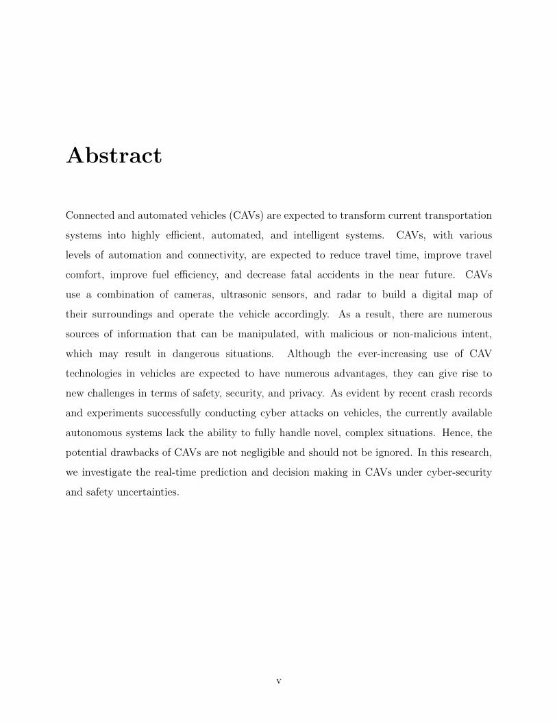
Abstract
Connected and automated vehicles (CAVs) are expected to transform current transportation
systems into highly efficient, automated, and intelligent systems. CAVs, with various
levels of automation and connectivity, are expected to reduce travel time, improve travel
comfort, improve fuel efficiency, and decrease fatal accidents in the near future. CAVs
use a combination of cameras, ultrasonic sensors, and radar to build a digital map of
their surroundings and operate the vehicle accordingly. As a result, there are numerous
sources of information that can be manipulated, with malicious or non-malicious intent,
which may result in dangerous situations. Although the ever-increasing use of CAV
technologies in vehicles are expected to have numerous advantages, they can give rise to
new challenges in terms of safety, security, and privacy. As evident by recent crash records
and experiments successfully conducting cyber attacks on vehicles, the currently available
autonomous systems lack the ability to fully handle novel, complex situations. Hence, the
potential drawbacks of CAVs are not negligible and should not be ignored. In this research,
we investigate the real-time prediction and decision making in CAVs under cyber-security
and safety uncertainties.
v

Table of Contents
Introduction 1
1 Real-Time Sensor Anomaly Detection and Identification in Automated
Vehicles 4
1.1 Introduction . . . . . . . . . . . . . . . . . . . . . . . . . . . . . . . . . . . . 7
1.2 Methods . . . . . . . . . . . . . . . . . . . . . . . . . . . . . . . . . . . . . . 12
1.2.1 Kalman Filter . . . . . . . . . . . . . . . . . . . . . . . . . . . . . . . 13
1.2.2 CNN . . . . . . . . . . . . . . . . . . . . . . . . . . . . . . . . . . . . 16
1.2.3 CNN-Empowered Kalman Filter (CNN-KF) . . . . . . . . . . . . . . 17
1.3 Data . . . . . . . . . . . . . . . . . . . . . . . . . . . . . . . . . . . . . . . . 18
1.4 Results . . . . . . . . . . . . . . . . . . . . . . . . . . . . . . . . . . . . . . . 20
1.4.1 Models Under a Single Anomaly Type . . . . . . . . . . . . . . . . . 21
1.4.2 Models Under Mixed Anomaly Types . . . . . . . . . . . . . . . . . . 27
1.5 Discussion . . . . . . . . . . . . . . . . . . . . . . . . . . . . . . . . . . . . . 31
1.6 Conclusion and Future Work . . . . . . . . . . . . . . . . . . . . . . . . . . . 33
2 Optimal Switching Policy Between Driving Entities in Semi-Autonomous
Vehicles 35
2.1 Introduction . . . . . . . . . . . . . . . . . . . . . . . . . . . . . . . . . . . . 37
2.2 Model Formulation . . . . . . . . . . . . . . . . . . . . . . . . . . . . . . . . 41
2.2.1 Under Full Information . . . . . . . . . . . . . . . . . . . . . . . . . . 41
2.2.2 Under Partial Information . . . . . . . . . . . . . . . . . . . . . . . . 46
2.3 Computational Study . . . . . . . . . . . . . . . . . . . . . . . . . . . . . . . 48
vi
2.3.1 Computational Study Under Full Information . . . . . . . . . . . . . 48
2.3.2 Computational Study Under Partial Information . . . . . . . . . . . . 62
2.4 Conclusion and Future Work . . . . . . . . . . . . . . . . . . . . . . . . . . . 65
3 A Dynamic Deep Reinforcement Learning-Bayesian Framework for Anomaly
Detection 68
3.1 Introduction . . . . . . . . . . . . . . . . . . . . . . . . . . . . . . . . . . . . 71
3.2 Methods . . . . . . . . . . . . . . . . . . . . . . . . . . . . . . . . . . . . . . 76
3.2.1 POMDP . . . . . . . . . . . . . . . . . . . . . . . . . . . . . . . . . . 77
3.2.2 A3C . . . . . . . . . . . . . . . . . . . . . . . . . . . . . . . . . . . . 79
3.3 Data . . . . . . . . . . . . . . . . . . . . . . . . . . . . . . . . . . . . . . . . 81
3.4 Results . . . . . . . . . . . . . . . . . . . . . . . . . . . . . . . . . . . . . . . 82
3.4.1 Performance Under Fixed Anomaly Rate . . . . . . . . . . . . . . . . 83
3.4.2 Performance Under Variable Anomaly Rate . . . . . . . . . . . . . . 84
3.4.3 An Illustrative Example . . . . . . . . . . . . . . . . . . . . . . . . . 88
3.5 Conclusion . . . . . . . . . . . . . . . . . . . . . . . . . . . . . . . . . . . . . 91
Conclusion 93
Bibliography 95
Appendices 107
A Summary of Key Literature and Notation for Chapter 1 . . . . . . . . . . . . 108
B Model Calibration . . . . . . . . . . . . . . . . . . . . . . . . . . . . . . . . . 111
Vita 113
vii

List of Tables
1.1 Detection performance of instant anomaly type for the KF, CNN and CNN-
KF models. . . . . . . . . . . . . . . . . . . . . . . . . . . . . . . . . . . . . 23
1.2 Detection performance of constant anomaly type for KF, CNN and CNN-KF
models. . . . . . . . . . . . . . . . . . . . . . . . . . . . . . . . . . . . . . . 23
1.3 Detection performance of gradual drift anomaly type for the KF, CNN and
CNN-KF models. . . . . . . . . . . . . . . . . . . . . . . . . . . . . . . . . . 25
1.4 Detection performance of bias anomaly type for KF, CNN and CNN-KF models. 25
1.5 Identification performance of training CNN models on one type of anomalous
sensor values and testing them to identify anomalous sensor values where all
anomaly types are present. The reported values are in percentages. . . . . . 29
1.6 Identification performance and the 95% CIs across 10 different executions for
all three models, at the anomaly rate of α = 5% and in the presence of all types
of anomalies. P-values indicate statistical significance at 5% level using paired
t-test and one-way ANOVA tests, between the identification performance of
all pairs of models. The reported values are in percentages. . . . . . . . . . . 30
1.7 Identification performance and the 95% CIs across 20 different executions for
all three models, at the anomaly rate of α = 1% and in the presence of all types
of anomalies. P-values indicate statistical significance at 5% level using paired
t-test and one-way ANOVA tests, between the identification performance of
all pairs of models. The reported values are in percentages. . . . . . . . . . 32
2.1 Comparison of the optimal policy with the two benchmark policies πI and πC . 53
viii

2.2 Mean percentage difference in total expected discounted cost, under the
optimal and benchmark policies for the 25 sample trips, starting from state
so. The 95% CI for the means are provided. . . . . . . . . . . . . . . . . . . 56
2.3 Mean total expected discounted cost, and mean percentage difference in total
expected discounted cost, under the optimal and benchmark policies for the
sample 25 trips, starting from state so, under Pl, P , and Ph. The 95% CI for
the means are provided. . . . . . . . . . . . . . . . . . . . . . . . . . . . . . 57
2.4 Mean percentage difference, and the corresponding 95% CI, in total expected
discounted risk of accident associated with the optimal and benchmark policies
of the sample 25 trips, starting from state so, under Pl, P , and Ph. . . . . . 58
2.5 The breakdown of risk of accident (mean and the corresponding 95% CI)
associated with the optimal policy for the sample 25 trips, starting from state
so, under Pl, P , and Ph. . . . . . . . . . . . . . . . . . . . . . . . . . . . . . 58
2.6 Mean percentage difference, and the corresponding 95% CI, between the
minimum total expected discounted risk of accident and the total expected
discounted risk of accident under benchmark policies for the sample 25 trips,
starting from state so, under Pl, P , and Ph. . . . . . . . . . . . . . . . . . 60
2.7 Mean total expected discounted cost, and mean percentage difference in
total expected discounted cost, under the optimal and benchmark policies
for the sample 25 trips starting from state so, under the corresponding sets
of probabilities of accident for the two driving entities. The 95% CI for the
means are provided. . . . . . . . . . . . . . . . . . . . . . . . . . . . . . . . 61
2.8 Mean difference in total expected discounted cost between V χ(s), πχ ∈
{π∗, πI , πC}, and U(s) for the sample 25 trips starting from state s0, for the
two extreme TPMs Pl and Ph. The 95% CI for the means are provided. . . 61
2.9 Total expected discounted cost under the A3C policy and benchmark policies,
starting from state zo. . . . . . . . . . . . . . . . . . . . . . . . . . . . . . . 65
2.10 Total expected discounted cost, WA(zo), under various degrees of observabil-
ity, starting from state zo. . . . . . . . . . . . . . . . . . . . . . . . . . . . . 65
ix

3.1 Hyperparameters utilized in the training of the A3C model. . . . . . . . . . 81
3.2 The mean and 95% CI anomaly detection performance of the bias anomaly
type for a fixed anomaly rate, ξ = 5%, and various trip lengths. P-values
indicate statistical significance at 5% level using paired t-tests, between the
F1 scores for the CNN and A3C models for all trip lengths. . . . . . . . . . 85
3.3 The mean and 95% CI anomaly detection performance of the gradual drift
anomaly type for a fixed anomaly rate, ξ = 5%, and various trip lengths. P-
values indicate statistical significance at 5% level using paired t-tests, between
the F1 scores for the CNN and A3C models for all trip lengths. . . . . . . . 85
3.4 The mean and 95% CI for F1 score of the CNN model, obtained for various
training and testing combinations of anomaly rate under bias anomaly type. 87
3.5 The mean and 95% CI for F1 score of the CNN model, obtained for various
training and testing combinations of anomaly rate under gradual drift anomaly
type. . . . . . . . . . . . . . . . . . . . . . . . . . . . . . . . . . . . . . . . . 87
3.6 The mean and 95% CI Anomaly detection performance of the bias anomaly
type for trip length T = 15000, and anomaly rate ξ ∈ {1%, 5%, 10%}. P-values
indicate statistical significance at 5% level using paired t-tests, between the
F1 scores for the CNN and A3C models for anomaly rates ξ ∈ {5%, 10%}. . 88
3.7 The mean and 95% CI Anomaly detection performance of the gradual drift
anomaly type for trip length T = 15000, and anomaly rate ξ ∈ {1%, 5%, 10%}.
P-values indicate statistical significance at 5% level using paired t-tests,
between the F1 scores for the CNN and A3C models for all anomaly rates,
ξ ∈ {1%, 5%, 10%}. . . . . . . . . . . . . . . . . . . . . . . . . . . . . . . . . 89
A.1 Summary of key literature related to anomaly detection in CAVs. . . . . . . 109
A.2 Summary of notation for Chapter 1. . . . . . . . . . . . . . . . . . . . . . . . 110
B.1 Parameter value generation for q(φ,µ) and ρ(µ) . . . . . . . . . . . . . . . . 112
x
List of Figures
1.1 Overview of the CNN-KF Framework. . . . . . . . . . . . . . . . . . . . . . 18
1.2 Illustrative example of the performance of KF, CNN, and CNN-KF models. . 31
2.1 An example MDP-generated optimal authority switching policy. . . . . . . . 50
2.2 A sample path of states under the optimal policy starting from state s =
([0, 0], I,−1). . . . . . . . . . . . . . . . . . . . . . . . . . . . . . . . . . . . 52
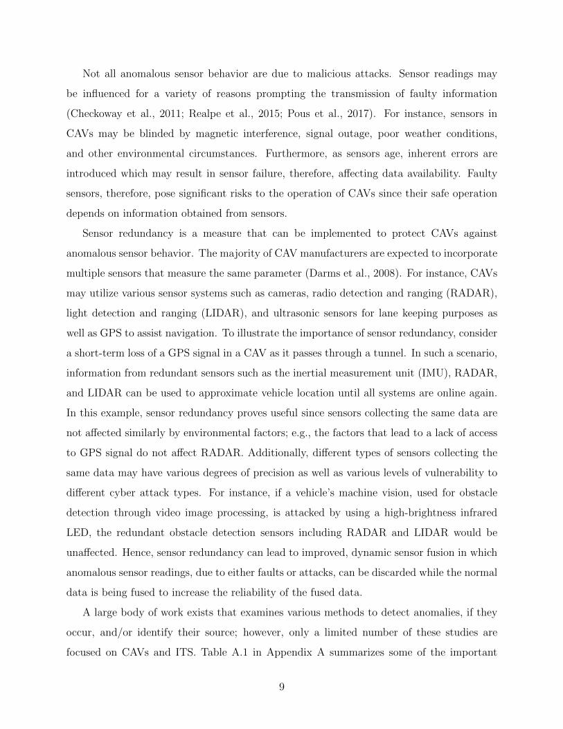
3.1 Overview of the anomaly detection framework. At each time epoch, the
sensor readings collected within the past several time epochs are used as an
input to the CNN model. The CNN model outputs the probability of the
sensor data being anomalous at each time epoch. Next, the CNN output
probabilities, plus a few additional problem-specific features, are fed into the
POMDP model as ‘imperfect observations.’ The POMDP model is solved to
(approximate) optimality using the A3C algorithm to obtain the policy that
prescribes the anomaly classification threshold for any given system belief
state, discriminating normal and anomalous sensor readings. . . . . . . . . . 77
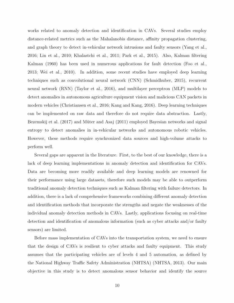
3.2 Illustration of data breakdown and flow of information. The CNN model is
trained and validated using CAV sensor data. The CNN model is then used
to generate probability streams of the system being anomalous on an internal
test set. These probabilities are used as observations in the POMDP model
trained by the A3C algorithm. Finally, an external test set is used to compare
the performance of the CNN-only and A3C models. . . . . . . . . . . . . . . 82
xi

3.3 Illustration of a sample path with a fixed anomaly rate and different trip
lengths. A fixed anomaly rate of ξ = 5% is used for trips with lengths of 5000,
15000, and 25000 epochs. . . . . . . . . . . . . . . . . . . . . . . . . . . . . . 84
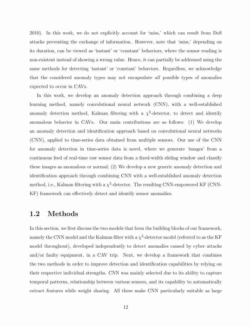
3.4 Illustration of a sample path with different rates of anomaly for road segments
with a fixed length. In this sample path, the CAV goes through three road
segments where it communicates with RSUs that can inject anomalies at
different rates, i.e., starting from ξ = 1%, anomaly rate first increases to
ξ = 10% and then decreases to ξ = 5%. . . . . . . . . . . . . . . . . . . . . 86
3.5 Illustration of a bias anomaly encountered in a sample path. The baseline
speed, baseline speed augmented with the anomaly, the CNN output proba-
bility, and the threshold specified by A3C are illustrated. . . . . . . . . . . 90
xii
Introduction
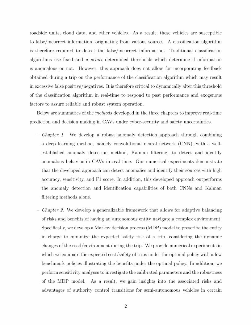
In Chapter 1, we investigate real-time sensor anomaly detection and identification in
CAVs. To navigate roadways, CAVs need to heavily rely on their sensor readings and the
information received from other vehicles, i.e., vehicle-to-vehicle (V2V) communication, and
roadside units, known as vehicle-to-infrastructure (V2I) communication. Hence, anomalous
sensor behavior/data points caused by either malicious cyber attacks or faulty vehicle sensors
can result in disruptive consequences, and possibly lead to fatal crashes. As a result, before
the mass implementation of CAVs, it is important to develop methodologies that can detect
anomalies and identify their sources seamlessly and in real-time.
Next in Chapter 2, we focus on the limitations of semi-autonomous vehicles under
certain circumstances where it is safer for the human driver to be in control compared
to the automated driving system. Such circumstances may be caused due to technological
failures, complex road and environmental conditions, or infrastructure deficiencies (e.g., lack
of roadside units or high-definition maps in certain areas), to name a few. Hence, for the
foreseeable future, the need for the transition of authority between the human driver and
the autonomous entity would continue to complicate traveling through the road network.
Switching control back and forth between the human driver and the autonomous driving
entity to maximize safety may not be straightforward as every such switch can itself pose a
short-term, elevated risk, especially under highly dynamic and stochastic traffic conditions.
As a result, we investigate the transfer of control authority in semi-autonomous vehicles to
improve overall road safety.
Lastly, in Chapter 3 we investigate real-time dynamic thresholding in classification
algorithms to adapt to complex road and environmental conditions. The successful operation
of CAVs are dependent on a large number of information sources such as on-board sensors,
1
roadside units, cloud data, and other vehicles. As a result, these vehicles are susceptible
to false/incorrect information, originating from various sources. A classification algorithm
is therefore required to detect the false/incorrect information. Traditional classification
algorithms use fixed and a priori determined thresholds which determine if information
is anomalous or not. However, this approach does not allow for incorporating feedback
obtained during a trip on the performance of the classification algorithm which may result
in excessive false positive/negatives. It is therefore critical to dynamically alter this threshold
of the classification algorithm in real-time to respond to past performance and exogenous
factors to assure reliable and robust system operation.
Below are summaries of the methods developed in the three chapters to improve real-time
prediction and decision making in CAVs under cyber-security and safety uncertainties.
– Chapter 1. We develop a robust anomaly detection approach through combining
a deep learning method, namely convolutional neural network (CNN), with a well-
established anomaly detection method, Kalman filtering, to detect and identify
anomalous behavior in CAVs in real-time. Our numerical experiments demonstrate
that the developed approach can detect anomalies and identify their sources with high
accuracy, sensitivity, and F1 score. In addition, this developed approach outperforms
the anomaly detection and identification capabilities of both CNNs and Kalman
filtering methods alone.
– Chapter 2. We develop a generalizable framework that allows for adaptive balancing
of risks and benefits of having an autonomous entity navigate a complex environment.
Specifically, we develop a Markov decision process (MDP) model to prescribe the entity
in charge to minimize the expected safety risk of a trip, considering the dynamic
changes of the road/environment during the trip. We provide numerical experiments in
which we compare the expected cost/safety of trips under the optimal policy with a few
benchmark policies illustrating the benefits under the optimal policy. In addition, we
perform sensitivity analyses to investigate the calibrated parameters and the robustness
of the MDP model. As a result, we gain insights into the associated risks and
advantages of authority control transitions for semi-autonomous vehicles in certain
2
conditions. We also develop a partially observable Markov decision process (POMDP)
model to account for cases when only partial information of the environmental risk is
available. We solve the POMDP using a state of the art deep reinforcement learning
technique, namely the asynchronous advantage actor critic (A3C) algorithm.
– Chapter 3. We develop a mathematical framework in which we pair an anomaly
classification algorithm, based on CNN, with a partially observable Markov decision
process (POMDP) model to determine the optimal dynamic threshold of an anomaly
classification algorithm to maximize the safety of a trip. We solve the resulting POMDP
model using the asynchronous advantage actor critic (A3C) deep reinforcement learning
algorithm. We provide numerical experiments in which we compare the performance
of the benchmark model, i.e., the CNN model with a fixed threshold, to the developed
POMDP model utilizing a dynamic threshold. The numerical experiments suggest that
the addition of the POMDP model improves the anomaly detection performance of the
CNN model, resulting in high accuracy, sensitivity, and positive predictive value. As a
result, we gain insights into the associated benefits and disadvantages of implementing
a dynamic classification threshold in response to complex exogenous factors.
3
Chapter 1
Real-Time Sensor Anomaly Detection
and Identification in Automated
Vehicles
4
Disclosure: This chapter is based on a paper published by van Wyk et al. (2019) in IEEE
Transactions on Intelligent Transportation Systems.
van Wyk, F., Wang, Y., Khojandi, A. and Masoud, N., 2019. Real-Time Sensor Anomaly
Detection and Identification in Automated Vehicles. IEEE Transactions on Intelligent
Transportation Systems.
My contributions to this paper include: (i) the development of the problem and
methodology to investigate the problem, (ii) reviewing the appropriate literature, (iii) the
identification of study objectives, (iv) collection of data, (v) design and conducting of the
numerical experiments, (vi) majority of the writing responsibilities of the manuscript.
Abstract
Connected and automated vehicles (CAVs) are expected to revolutionize the transportation
industry, mainly through allowing for a real-time and seamless exchange of information
between vehicles and roadside infrastructure. Although connectivity and automation are
projected to bring about a vast number of benefits, they can give rise to new challenges in
terms of safety, security, and privacy. To navigate roadways, CAVs need to heavily rely on
their sensor readings and the information received from other vehicles and roadside units.
Hence, anomalous sensor readings caused by either malicious cyber attacks or faulty vehicle
sensors can result in disruptive consequences, and possibly lead to fatal crashes. As a result,
before the mass implementation of CAVs, it is important to develop methodologies that can
detect anomalies and identify their sources seamlessly and in real-time. In this work, we
develop an anomaly detection approach through combining a deep learning method, namely
convolutional neural network (CNN), with a well-established anomaly detection method,
Kalman filtering with a χ2-detector, to detect and identify anomalous behavior in CAVs.
Our numerical experiments demonstrate that the developed approach can detect anomalies
and identify their sources with high accuracy, sensitivity, and F1 score. In addition, this
developed approach outperforms the anomaly detection and identification capabilities of
both CNNs and Kalman filtering with a χ2-detector methods alone. It is envisioned that
5

this research will contribute to the development of safer and more resilient CAV systems
that implement a holistic view towards intelligent transportation system (ITS) concepts.
6
1.1 Introduction
Our current transportation system is on the brink of transforming into a highly connected,
automated, and intelligent system as a result of the rapid emergence of connected and
automated vehicles (CAVs) (Ran and Boyce, 2012). CAVs, with various degrees of
connectivity and automation, are expected to play an integral role in the next phase
of the transportation revolution, leading to more accessible, more efficient, safer, more
environmentally friendly, and hence sustainable, transportation options (Meyer and Beiker,
2014; Litman, 2017). CAVs use wireless technology to facilitate communication between
vehicles, with roadside units (RSUs), and with personal mobile devices. This will
allow them to continuously transmit and share information such as speed, position,
acceleration, and braking, enabling CAVs to warn their surrounding vehicles of potentially
unsafe circumstances. These vehicle-to-vehicle (V2V) and vehicle-to-infrastructure (V2I)
communication technologies will provide unprecedented efficiency, safety, and mobility
advancements. For instance, CAV technologies are expected to decrease fatal traffic accidents
by as much as 80%, reducing their corresponding $870 billion cost, while also improving
traffic flow, cutting into the approximate 7 billion hours American motorists spend in traffic
annually (USDOT, 2016).
Although the ever-increasing use of CAV technologies in vehicles are expected to have
numerous advantages, the potential drawbacks are not negligible. CAVs use a variety of
sensors to build a virtual map of their surroundings in order to drive in the correct lane
within the speed limit, avoid collisions, and detect obstacles in their immediate physical
environment. Hence, anomalous sensor values caused by either malicious cyber attacks
or faulty vehicle sensors can result in disruptive consequences, and possibly lead to fatal
crashes. The increase in connectivity and automation has led to the scrutiny of in-vehicle
network architectures used by automotive manufacturers and evaluation of vulnerabilities
in their resiliency against such anomalous behavior (Koscher et al., 2010; Greenberg, 2015;
Weimerskirch and Gaynier, 2015). For instance, the dedicated short-range communication
(DSRC) technology is currently used to facilitate communication within connected networks.
7
DSRC has a range of approximately 300 meters, hence it can protect vehicles from long-
range cyber attacks, e.g., a stationary attacker would only have a short time-window to
attack moving vehicles when they are in close proximity (Bai et al., 2010). Although such a
technology can prove useful, it is not comprehensive enough and leaves CAVs vulnerable to
non-stationary attackers, among others. Hence, it is necessary to better understand CAVs’
vulnerabilities and develop holistic, real-time methodologies that can mitigate them.
Various internal and external cyber attack surfaces exist in CAV systems, i.e., the
entry point of the attack, which may enable hackers to access and compromise the safety
and integrity of CAVs (Koscher et al., 2010; Checkoway et al., 2011; Greenberg, 2015;
Weimerskirch and Gaynier, 2015; Petit and Shladover, 2015; Yan et al., 2016; Field, 2017).
Typical internal attack surfaces include in-vehicle devices, GPS system, on-board diagnostics
(OBD) system, vehicle sensors including the controller area network (CAN) bus, and other
sensors required for CAV operation. For instance, Checkoway et al. (2011) demonstrated
through an OBD port attack, it is possible to disable the brakes, turn-off head-lights, and
take over steering for cars equipped with a low level of autonomy. Typical external attack
surfaces include information from RSUs, machine vision, data from other vehicles, security
system breaches of the vehicle, and navigation interference (Field, 2017; Jo et al., 2016;
Truong et al., 2005). For instance, Field (2017) demonstrated how an attacker could gain
access to the visual recognition software used in autonomous vehicles and manipulate it by
creating a simple alteration to RSUs that would cause the car to misinterpret them, possibly
putting vehicle occupants at risk. Similarly, several teams have hacked traffic light controller
systems, highway signs, and traffic surveillance cameras (Huq et al., 2017). For instance, in
2017, approximately 70% of the storage devices that record data from Washington D.C. police
surveillance cameras were infected with ransomware by hackers (Williams, 2017). Injection of
fake information and map database poisoning is considered to be one of the most dangerous
cyber attacks on CAVs (Petit and Shladover, 2015). Future CAVs are expected to have even
more attack surfaces than what has currently been investigated. Possible reasons for cyber
attacks on CAVs include financial gain, collecting private information, and gaining priority
access to infrastructure.
8
Not all anomalous sensor behavior are due to malicious attacks. Sensor readings may
be influenced for a variety of reasons prompting the transmission of faulty information
(Checkoway et al., 2011; Realpe et al., 2015; Pous et al., 2017). For instance, sensors in
CAVs may be blinded by magnetic interference, signal outage, poor weather conditions,
and other environmental circumstances. Furthermore, as sensors age, inherent errors are
introduced which may result in sensor failure, therefore, affecting data availability. Faulty
sensors, therefore, pose significant risks to the operation of CAVs since their safe operation
depends on information obtained from sensors.
Sensor redundancy is a measure that can be implemented to protect CAVs against
anomalous sensor behavior. The majority of CAV manufacturers are expected to incorporate
multiple sensors that measure the same parameter (Darms et al., 2008). For instance, CAVs
may utilize various sensor systems such as cameras, radio detection and ranging (RADAR),
light detection and ranging (LIDAR), and ultrasonic sensors for lane keeping purposes as
well as GPS to assist navigation. To illustrate the importance of sensor redundancy, consider
a short-term loss of a GPS signal in a CAV as it passes through a tunnel. In such a scenario,
information from redundant sensors such as the inertial measurement unit (IMU), RADAR,
and LIDAR can be used to approximate vehicle location until all systems are online again.
In this example, sensor redundancy proves useful since sensors collecting the same data are
not affected similarly by environmental factors; e.g., the factors that lead to a lack of access
to GPS signal do not affect RADAR. Additionally, different types of sensors collecting the
same data may have various degrees of precision as well as various levels of vulnerability to
different cyber attack types. For instance, if a vehicle’s machine vision, used for obstacle
detection through video image processing, is attacked by using a high-brightness infrared
LED, the redundant obstacle detection sensors including RADAR and LIDAR would be
unaffected. Hence, sensor redundancy can lead to improved, dynamic sensor fusion in which
anomalous sensor readings, due to either faults or attacks, can be discarded while the normal
data is being fused to increase the reliability of the fused data.
A large body of work exists that examines various methods to detect anomalies, if they
occur, and/or identify their source; however, only a limited number of these studies are
focused on CAVs and ITS. Table A.1 in Appendix A summarizes some of the important
9
works related to anomaly detection and identification in CAVs. Several studies employ
distance-related metrics such as the Mahalanobis distance, affinity propagation clustering,
and graph theory to detect in-vehicular network intrusions and faulty sensors (Yang et al.,
2016; Lin et al., 2010; Khalastchi et al., 2011; Park et al., 2015). Also, Kalman filtering
Kalman (1960) has been used in numerous applications for fault detection (Foo et al.,
2013; Wei et al., 2010). In addition, some recent studies have employed deep learning
techniques such as convolutional neural network (CNN) (Schmidhuber, 2015), recurrent
neural network (RNN) (Taylor et al., 2016), and multilayer perceptron (MLP) models to
detect anomalies in autonomous agriculture equipment vision and malicious CAN packets in
modern vehicles (Christiansen et al., 2016; Kang and Kang, 2016). Deep learning techniques
can be implemented on raw data and therefore do not require data abstraction. Lastly,
Bezemskij et al. (2017) and Muter and Asaj (2011) employed Bayesian networks and signal
entropy to detect anomalies in in-vehicular networks and autonomous robotic vehicles.
However, these methods require synchronized data sources and high-volume attacks to
perform well.
Several gaps are apparent in the literature. First, to the best of our knowledge, there is a
lack of deep learning implementations in anomaly detection and identification for CAVs.
Data are becoming more readily available and deep learning models are renowned for
their performance using large datasets, therefore such models may be able to outperform
traditional anomaly detection techniques such as Kalman filtering with failure detectors. In
addition, there is a lack of comprehensive frameworks combining different anomaly detection
and identification methods that incorporate the strengths and negate the weaknesses of the
individual anomaly detection methods in CAVs. Lastly, applications focusing on real-time
detection and identification of anomalous information (such as cyber attacks and/or faulty
sensors) are limited.
Before mass implementation of CAVs into the transportation system, we need to ensure
that the design of CAVs is resilient to cyber attacks and faulty equipment. This study
assumes that the participating vehicles are of levels 4 and 5 automation, as defined by
the National Highway Traffic Safety Administration (NHTSA) (NHTSA, 2013). Our main
objective in this study is to detect anomalous sensor behavior and identify the source
10

anomalous sensor in real-time for CAVs to assure the high reliability of fused data. Our
framework is generic in that a ‘sensor’ may refer to any of the on-board sensors in a CAV, or
another connected vehicle or roadside unit (RSU) that is communicating with the CAV.
Specifically, we develop a holistic and generic framework by combining a deep learning
technique, i.e., CNN, and Kalman filtering with a χ2-detector, and investigate their ability to
detect and identify various types of anomalous behavior in real-time. In addition, we perform
various experiments to investigate the effects of anomaly type, magnitude, and duration.
Anomalous sensor readings, caused by attacks or failures, can present themselves in
different ways. Several network attack taxonomies are available in the literature. Bhuyan
et al. (2014) summarize the taxonomy of intrusions or attacks in computer network systems,
which encompass CAVs. Also, several faulty sensor behaviors are discussed in (Sharma
et al., 2010). We consider the anomalous sensor behavior resulting from both false injection
attacks and sensor failures. According to the literature, anomalous sensor behavior can be
represented by the five main following types:
1. Instant: A sharp, unexplained change in the observed data between two successive
sensor readings.
2. Constant: A temporarily constant observation that is different from the “normal”
sensor readings and is uncorrelated to the underlying physical phenomena.
3. Gradual drift: A small and gradual drift in observed data during a time period. It
can result in a large discrepancy between the observed data and the true state of the
system in time.
4. Bias: A temporarily constant offset from the sensor readings.
5. Miss: Lack of available data during a time period.
In this work, consistent with literature (Bhuyan et al., 2014; Sharma et al., 2010), we
focus on detection and identification of anomalous behavior, caused by either cyber attacks
or faulty sensors, resulting in ‘instant,’ ‘constant,’ ‘gradual drift,’ and ‘bias.’ These types of
anomalies are some of the most dangerous for CAVs (Petit and Shladover, 2015; Mo et al.,
11
2010). In this work, we do not explicitly account for ‘miss,’ which can result from DoS
attacks preventing the exchange of information. However, note that ‘miss,’ depending on
its duration, can be viewed as ‘instant’ or ‘constant’ behaviors, where the sensor reading is
non-existent instead of showing a wrong value. Hence, it can partially be addressed using the
same methods for detecting ‘instant’ or ‘constant’ behaviors. Regardless, we acknowledge
that the considered anomaly types may not encapsulate all possible types of anomalies
expected to occur in CAVs.
In this work, we develop an anomaly detection approach through combining a deep
learning method, namely convolutional neural network (CNN), with a well-established
anomaly detection method, Kalman filtering with a χ2-detector, to detect and identify
anomalous behavior in CAVs. Our main contributions are as follows: (1) We develop
an anomaly detection and identification approach based on convolutional neural networks
(CNN), applied to time-series data obtained from multiple sensors. Our use of the CNN
for anomaly detection in time-series data is novel, where we generate ‘images’ from a
continuous feed of real-time raw sensor data from a fixed-width sliding window and classify
these images as anomalous or normal; (2) We develop a new generic anomaly detection and
identification approach through combining CNN with a well-established anomaly detection
method, i.e., Kalman filtering with a χ2-detector. The resulting CNN-empowered KF (CNN-
KF) framework can effectively detect and identify sensor anomalies.
1.2 Methods
In this section, we first discuss the two models that form the building blocks of our framework,
namely the CNN model and the Kalman filter with a χ2-detector model (referred to as the KF
model throughout), developed independently to detect anomalies caused by cyber attacks
and/or faulty equipment, in a CAV trip. Next, we develop a framework that combines
the two methods in order to improve detection and identification capabilities by relying on
their respective individual strengths. CNN was mainly selected due to its ability to capture
temporal patterns, relationship between various sensors, and its capability to automatically
extract features while weight sharing. All these make CNN particularly suitable as large
12
amounts of data are becoming available. However, there is always a risk of unknown/unseen
patterns going undetected when relying only on CNNs. Hence, using an architecture that
combines CNN and KF can provide an additional level of reliability for the task at hand, as
CNN and KF are complementary in their ability to detect anomalies. It is worth noting that
we also explored recurrent neural networks (RNNs) with long short-term memory (LSTM)
units; however, CNN consistently outperformed RNN in all preliminary experiments. This
is partly because in this particular application, there are many normal values between
consecutive anomalous values, which generally makes it hard for RNN to distinguish between
anomalous and normal values in an extended sequence of data (Malhotra et al., 2015).
In general, the inputs to the model are the data collected from sensors, reading the
same or highly correlated physical quantities. Based on the input data, at every time step,
e.g., a few milliseconds (ms), outputs are generated as to whether anomalies are present
(detection) and if so, which sensor reading(s) are erroneous (identification). Consequently,
erroneous data can be excluded and normal data can be seamlessly fused to support CAV
operation. Please note that all notation used are summarized in Table A.2 in Appendix A.
1.2.1 Kalman Filter
As discussed, Kalman filter combined with a failure detector is a well-established, widely
used method for fault detection and identification in time-series data. In order to detect and
identify anomalous sensor readings, we use an adaptive Kalman filter with a χ2-detector to
filter out process and measurement noise. Specifically, we assume our physical system is a
discrete-time linear time-invariant system in the following form:
x(k) = Ax(k − 1) + w(k − 1) (1.1)
where x(k) ∈ Rm is the vector of state variables at time k, w(k) ∈ Rm is the process noise
at time k, and A ∈ Rm×m is the state-transition matrix.
As discussed, we consider redundant sensor in this study. Let n denote the number of
these sensors. That is, we consider n local subsystems, corresponding to the redundant
13

sensors, with measurement matrices H(k) ∈ Rp×m and sensing model:
zi(k) = H(k)x(k) + vi(k), i = 1, 2, ..., n (1.2)
where vi(k) ∈ Rp is zero mean Gaussian white noise sequences associated with the process
and the measurement. The covariance matrices of vi(k) ∈ Rp and w(k) are Ri(k) and
Q(k), respectively. We assume vi(k) and w(k) are independent. In equation (1.2),
zi(k) = [zi,1(k), zi,2(k), ..., zi,p(k)]T ∈ Rp is a vector of sensor measurements for subsystem
i ∈ {1, ..., n}. We assume all n subsystems have the same measurement matrix H(k) and
the readings across all subsystems are synchronized.
For each subsystem, a Kalman filter is used to estimate the state vector x(k) from
sensor reading zi(k). Kalman filter consists of two phases, i.e. prediction and update. The
prediction phase advances the state estimate before the next measurement, and the update
phase corrects the state estimate based on the measurement.
Let z(k|k − 1) denote the predicted value of measurement at time k, P (k|k − 1) denotes
the error covariance matrix of predicted state, and ν(k) denote the innovation, i.e., the
difference between the measurement z(k) and the predicted value of measurement at time k,
ν(k) = z(k)− z(k|k − 1). (1.3)
Also let S(k) denote covariance matrix of innovation. In practice, covariance matrices R and
Q are generally unknown a priori. Thus, we apply an adaptive Kalman filter to approximate
these matrices (Mohamed and Schwarz, 1999). Specifically, we use a moving estimation
window of size M to adaptively estimate R and Q matrices according to the innovation
sequence within the time window, i.e.,
R(k) = Cν(k)−H(k)P (k|k − 1)H(k)T ,
Q(k) = K(k)Cν(k)K(k)T ,(1.4)
where
Cν(k) =1
M
k−1∑j=k−M
ν(j)ν(j)T . (1.5)
14
We use a χ2-detector to construct χ2 test statistics, to determine whether the new
measurement falls into the gate region with the probability determined by the gate threshold
γ, defined as
Vγ(k) = {z :(z − z(k|k − 1))TS(k)−1(z − z(k|k − 1)) ≤ γ}. (1.6)
The χ2 test statistics for each local subsystem is defined as
t(k) = ν(k)TS(k)−1ν(k) (1.7)
It is easy to show that under Gaussian assumption the test statistic has a χ2 distribution
with p degrees of freedom, where p is the number of components of the measurement vector.
However, in practice, usually w and vi do not follow Gaussian distributions, and parameter
γ has to be selected empirically. Hence, the threshold γ for t(k) and the time window size
M can be tuned.
Selection of the threshold γ is a trade-off between sensitivity of the trained model (i.e., the
proportion of correctly identified anomalies), and the false-alarm rate. For each experiment
in our experiment section, we select γ using a grid search within the range {1, 2, ..., 50}, and
select the value of γ resulting in the highest F1 score.
The window size M is a parameter that allows for the control of smoothing short-term
fluctuations in the detector. To select the best value for M , we performed a grid search.
Specifically, for various values of M in our grid search, we computed the Area Under the
ROC Curve (AUC) on a validation dataset. The results suggested that M ∈ {10, 15, 20}
provides robust results and high AUC (≈ 0.96). The AUC values within this range are
similar. Hence, consistent with previously published work (e.g., Loebis et al. (2004)), we
selected the window size M = 15 epochs for our experiments.
Once a faulty measurement stream has been identified, in order to ensure the future
estimate is reliable, the measurement stream should be rejected at once and not fused with
other measurements to ensure that the information generated through data fusion is not
contaminated.
15

1.2.2 CNN
To apply CNN for real-time detection and identification of anomalous sensor behavior, we use
a fixed-width sliding window on input data from all sensors measuring the same quantity,
either directly or indirectly, where conversions or combining with other sensors may be
required to infer the value of the quantity. At every epoch, as new observations are collected
from sensors, the sliding window shifts to include these latest observations. Hence, the input
to CNN is a series of ‘images’ from the continuous feed of raw sensor data during a CAV
trip. For instance, consider three sensors (e.g., GPS, accelerometer, and transmission vehicle
speed sensor) measuring vehicle speed at the sampling interval of 0.1 seconds. Hence, an
image of size 3×10 would include the data collected from the three sensors during the last one
second of the trip. The CNN therefore utilizes the data from multiple sensors simultaneously
for detection and identification of anomalous values.
CNN models are trained to evaluate these images to detect and identify anomalies in real-
time. Specifically, a sliding window is used on retrospectively collected data from sensors to
produce images for training and testing. Because the goal is both to detect and to identify
anomalies, for each sensor we train a separate model using labeled images, i.e., supervised
learning. That is, if an anomaly is present in an image constructed with the data from the
sensor of interest, the response variable is set to 1; otherwise, it is set equal to 0. Once
separate models are trained to identify anomalies for each sensor, a logical OR operator on
the outcomes of the all such models determines whether anomalous readings are detected
across all sensors.
In our experiments, for each CNN model, a popular image recognition architecture
from the literature is adopted (Krizhevsky et al., 2012). The parameter values for this
architecture are then selected based on a number of experiments performed to maximize
anomaly detection and identification performance on a validation set. In short, we used
three convolution layers with max-pooling, followed by two fully connected layers with
random dropout between the layers. A 1 × 2 pool size is used and 40, 60, and 60 filters
are used for convolutional layers one to three, respectively. Also, a random dropout rate of
0.1 and batch size of 128 is used to train the CNN models. Furthermore, rectified linear
16
unit (ReLU) activation functions are used and the Adam optimizer for Tensorflow in Python
is implemented to minimize binary cross-entropy (Kingma and Ba, 2014). The following
parameters were used for the Adam optimization algorithm: learning rate, α = 0.001,
exponential decay rates, β1 = 0.9, β2 = 0.999, and a fuzz factor, ε = 10−8.
It is widely acknowledged that deep learning models such as CNNs are often subject
to ‘overfitting’ during the training process (Krizhevsky et al., 2012; Srivastava and
Salakhutdinov, 2014). To reduce the risk of overfitting, in addition to random dropouts,
we use early stopping to monitor the accuracy of the validation set with a patience of 200
epochs. Therefore, when training a CNN model, starting from any training epoch, if the
validation accuracy during the following 200 epochs does not increase, training is terminated
and the model corresponding to 200 training epochs ago, which resulted in the highest
validation accuracy, is selected.
1.2.3 CNN-Empowered Kalman Filter (CNN-KF)
In order to further improve upon the detection and identification performances of the
individual KF and CNN models, we develop a new framework that relies on both CNN
and Kalman filter as shown in Figure 1.1. In this framework, first CNN models process the
images of raw data from all sensors, which are obtained by using a sliding window over all
sensor readings, to identify whether the readings from each sensor are normal or anomalous.
Consequently, the sensors with anomalous behavior are excluded and the readings from
normal sensors are separately fed into adaptive Kalman filters with failure detectors for
further examination and anomaly detection. If Kalman filter detects anomalies that are
missed by CNN, the readings from the corresponding sensors are excluded and the remaining
normal data are fused in order to achieve a higher degree of reliability. As time passes and the
vehicle continues its trip, if the sensors that presented anomalies go back to normal behavior,
as verified by both CNN models and Kalman filters, the exclusion is no longer necessary and
hence, the readings of the previously excluded sensors would be used in fusion again. In
this study, we use a CNN-empowered Kalman Filter (CNN-KF), as opposed to a Kalman
Filter empowered CNN (KF-CNN), mainly because having the Kalman filter in the last layer
of learning allows for the reliable fusion of the non-anomalous sensor values (Schmidhuber,
17
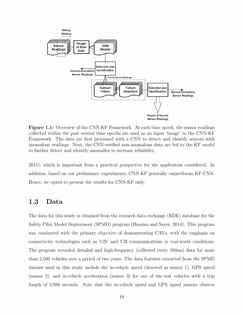
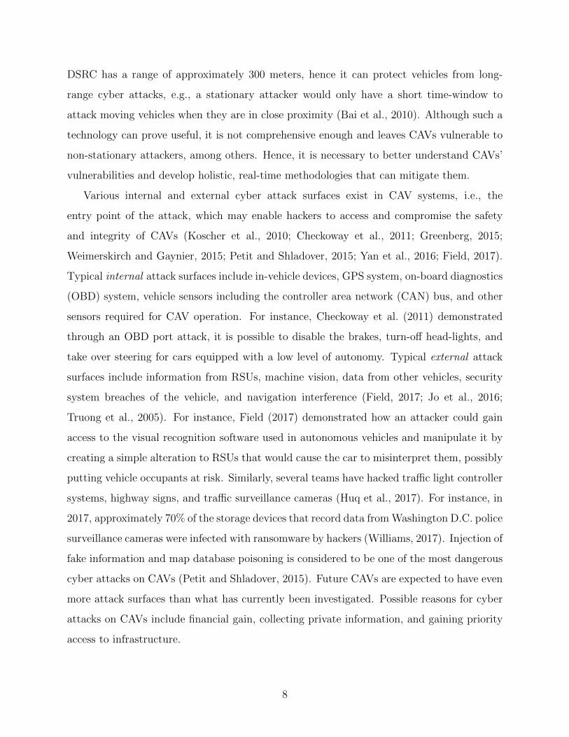
Figure 1.1: Overview of the CNN-KF Framework. At each time epoch, the sensor readingscollected within the past several time epochs are used as an input ‘image’ to the CNN-KFFramework. The data are first processed with a CNN to detect and identify sensors withanomalous readings. Next, the CNN-verified non-anomalous data are fed to the KF modelto further detect and identify anomalies to increase reliability.
2015), which is important from a practical perspective for the application considered. In
addition, based on our preliminary experiments, CNN-KF generally outperforms KF-CNN.
Hence, we opted to present the results for CNN-KF only.
1.3 Data
The data for this study is obtained from the research data exchange (RDE) database for the
Safety Pilot Model Deployment (SPMD) program (Bezzina and Sayer, 2014). This program
was conducted with the primary objective of demonstrating CAVs, with the emphasis on
connectivity technologies such as V2V and V2I communications in real-world conditions.
The program recorded detailed and high-frequency (collected every 100ms) data for more
than 2,500 vehicles over a period of two years. The data features extracted from the SPMD
dataset used in this study include the in-vehicle speed (denoted as sensor 1), GPS speed
(sensor 2), and in-vehicle acceleration (sensor 3) for one of the test vehicles with a trip
length of 2,980 seconds. Note that the in-vehicle speed and GPS speed sensors observe
18
the same quantity, namely, speed, whereas the acceleration sensor observes the vehicle’s
acceleration which can be used to infer speed.
Since there are no publicly available datasets for CAVs that include anomalies in sensor
measurements, due to either attacks or faults, and the ground truths, we used simulation to
generate datasets for our experiments. Specifically, we accounted for the four major anomaly
types including instant, constant, gradual drift, and bias. We inject all four types of anomaly
into each of the three speed-related (redundant) sensors. We assume the onset of anomalous
values in sensors, due to either attacks or faults, occur independently. That is, we do
not explicitly train models on datasets containing interdependent sensor failures or systemic
cyber attacks on vehicle sensors. Additionally, we assume that no more than one anomaly can
start in every time epoch, which is indeed very unlikely considering that sensors are generally
reliable, and attacks/faults to sensors occur independently. However, dependent on the types,
onset times, and durations of anomalies, multiple sensors may be anomalous at the same time.
There is existing work that illustrates the sensors considered in our numerical study, i.e.,
speed and acceleration sensors, are vulnerable to cyber attacks or faults (e.g., see Petit and
Shladover (2015), Trippel et al. (2017), Currie (2015)). For in-vehicle speed and acceleration
sensors, an injection attack through the CAN bus or the on-board diagnostics (OBD) system,
could give rise to the four types of anomalies considered in this work. Also, for the in-vehicle
acceleration sensor, an acoustic injection attack could result in anomalous sensor values.
Lastly, for the speed measurement from the GPS, both the operating environment of the
vehicle and GPS spoofing/jamming attacks may result in anomalous sensor values.
We generate various datasets for our experiments at 1% or 5% rates of anomalies, denoted
by α. We simulate the anomalies to occur at randomly selected onset times (discretized
into 100ms) to randomly selected sensors. To simulate the corresponding attacks/faults,
these anomalies are then added to each affected sensor’s ‘base value,’ i.e., the normal sensor
readings in the original dataset indicating the traveling speed of the CAV at the time that
the anomaly was introduced. Algorithm 1 presents the pseudo code used for simulating
the anomalies. Note that vectors Vi and V ′i , i ∈ {1, 2, . . . , n}, denote non-anomalous and
anomalous readings for sensor i, respectively. To facilitate thorough experiments, we vary
the simulated anomalies in type, magnitude and/or duration when generating the datasets.
19
In addition, dependent on the experiment, we generate datasets where we randomly sample
from a set of one or all anomaly types. The exact types of anomalies considered as well as
their magnitude (and duration) will be discussed in detail for each experiment in Section
1.4.
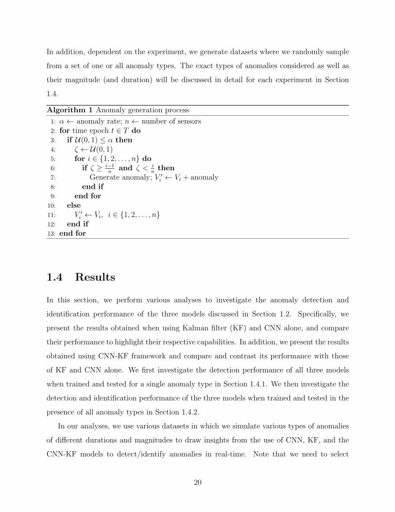
Algorithm 1 Anomaly generation process
1: α← anomaly rate; n← number of sensors2: for time epoch t ∈ T do3: if U(0, 1) ≤ α then4: ζ ← U(0, 1)5: for i ∈ {1, 2, . . . , n} do6: if ζ ≥ i−1
nand ζ < i
nthen
7: Generate anomaly; V ′i ← Vi + anomaly8: end if9: end for
10: else11: V ′i ← Vi, i ∈ {1, 2, . . . , n}12: end if13: end for
1.4 Results
In this section, we perform various analyses to investigate the anomaly detection and
identification performance of the three models discussed in Section 1.2. Specifically, we
present the results obtained when using Kalman filter (KF) and CNN alone, and compare
their performance to highlight their respective capabilities. In addition, we present the results
obtained using CNN-KF framework and compare and contrast its performance with those
of KF and CNN alone. We first investigate the detection performance of all three models
when trained and tested for a single anomaly type in Section 1.4.1. We then investigate the
detection and identification performance of the three models when trained and tested in the
presence of all anomaly types in Section 1.4.2.
In our analyses, we use various datasets in which we simulate various types of anomalies
of different durations and magnitudes to draw insights from the use of CNN, KF, and the
CNN-KF models to detect/identify anomalies in real-time. Note that we need to select
20
the parameter γ for KF models and also extensively train CNN models and tune their
many parameters. Hence, for any given dataset, we use a training/validation/testing split of
60%/20%/20%. We use the training and validation sets to tune the model parameters. Next,
to objectively evaluate their performance levels, we use the separate test sets for testing.
We evaluate the performance of the models in terms of accuracy, sensitivity, precision,
and F1 score. Accuracy measures the overall proportion of correct predictions for normal and
anomalous sensor values. Sensitivity assesses the proportion of correctly identified anomalous
sensor values from the total number of anomalous sensor values. Precision measures the
proportion of anomalous sensor values among those predicted as anomalous. Lastly, F1
score is the harmonic mean of sensitivity and precision. These metrics are particularly
chosen as they measure the ability of the models to correctly differentiate between normal
and anomalous sensor behavior. Note that these metrics are commonly used to evaluate the
performance of classification models. Here, for consistency and to enable comparison of all
models, we use the same metrics to evaluate the performance of CNN, KF, and CNN-KF
models.
1.4.1 Models Under a Single Anomaly Type
In this section we compare the detection performance of the three models for the specific
types of anomalies, as discussed in Section 1.1, namely, instant, constant, gradual drift, and
bias. We generate various datasets, each with a specific type of anomaly, with anomaly rate
α = 5%. For each dataset, we train and test CNN models to measure their performance in
detecting the specific anomaly type. Because each sensor reading in our experiment is one
dimensional, the state transition matrix A and measurement matrix H for KF are simply
single values.
Instant
The instant anomaly type is simulated as a random Gaussian variable with mean and variance
of zero and 0.01, respectively, that is scaled by a scalar c ∈ {25, 100, 500, 1,000, 10,000},
21
i.e., c × N (0, 0.01), to capture various magnitudes. The resulting simulated value is added
to the base value of sensor measurement for one epoch, i.e., 100 ms.
Table 1.1 illustrates the anomaly detection performance of the KF, CNN, and CNN-KF
models. Considering the detection performance of KF and CNN models, the following is
noted. In general the detection performance of the KF and CNN models increases across all
metrics in the magnitude of the instant anomaly type, which is consistent with the intuition.
For small magnitudes of anomalous sensor values, i.e., the first two rows in Table 1.1, the
detection performance of the models are poor. However, in these cases the difference between
the anomalous sensor values and non-anomalous sensor values are generally too small to
pose any substantial risks to the operation of the vehicle. For magnitudes that may pose
significant risk to the operation of the vehicle, i.e., rows 3–5, the models are able to detect
anomalous behavior with high performance. As seen in the table, KF and CNN models
have similar performance for instant anomalies with large magnitudes. The CNN models
generally outperform KF models in terms of sensitivity, precision, and F1 score. Particularly,
sensitivity is higher in CNN models, which can directly impact the reliability and safety of
fused data in CAVs. A reason for this higher performance of CNN models compared to KF
models is that when the anomalies are small enough, the attack will fall into the region of
gating for the KF model, therefore it cannot be detected by the chi-square test, which results
in a low sensitivity measure. Additionally, unlike the KF models that use the readings by a
single sensor over time to detect any potential anomalies on that sensor, the CNN models use
the readings from all sensors within a time window to detect anomalous behavior by each
individual sensor. This redundancy in information improves the CNN performance when the
anomaly magnitudes are small and therefore harder to detect.
Considering the anomaly detection performance of the CNN-KF model for the instant
anomaly type, the following is noted. Similar to the results for KF and CNN models, the
detection performance across all metrics increases in anomaly magnitude. Furthermore, it
is seen that, in general, the CNN-KF model improves upon the detection performance of
both KF and CNN models as reported in Table 1.1. For instance, for instant anomalies of
magnitude 25×N (0, 0.01) added to the base value (row 1), it is seen that sensitivity and F1
score of the CNN-KF model respectively increase by 13.1% and 18.9% over the KF model,
22
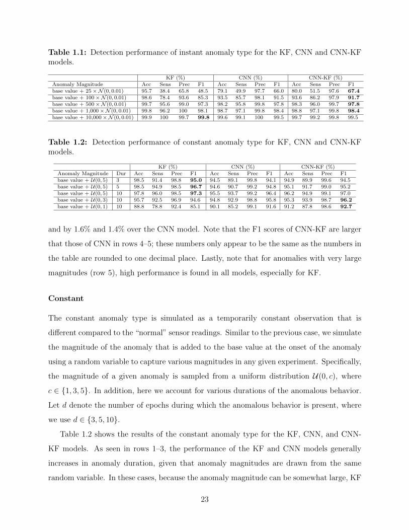
Table 1.1: Detection performance of instant anomaly type for the KF, CNN and CNN-KFmodels.
KF (%) CNN (%) CNN-KF (%)Anomaly Magnitude Acc Sens Prec F1 Acc Sens Prec F1 Acc Sens Prec F1base value + 25×N (0, 0.01) 95.7 38.4 65.8 48.5 79.1 49.9 97.7 66.0 80.0 51.5 97.6 67.4base value + 100×N (0, 0.01) 98.6 78.4 93.6 85.3 93.5 85.7 98.1 91.5 93.6 86.2 97.9 91.7base value + 500×N (0, 0.01) 99.7 95.6 99.0 97.3 98.2 95.8 99.8 97.8 98.3 96.0 99.7 97.8base value + 1,000×N (0, 0.01) 99.8 96.2 100 98.1 98.7 97.1 99.8 98.4 98.8 97.1 99.8 98.4base value + 10,000×N (0, 0.01) 99.9 100 99.7 99.8 99.6 99.1 100 99.5 99.7 99.2 99.8 99.5
Table 1.2: Detection performance of constant anomaly type for KF, CNN and CNN-KFmodels.
KF (%) CNN (%) CNN-KF (%)Anomaly Magnitude Dur Acc Sens Prec F1 Acc Sens Prec F1 Acc Sens Prec F1base value + U(0, 5) 3 98.5 91.4 98.8 95.0 94.5 89.1 99.8 94.1 94.9 89.9 99.6 94.5base value + U(0, 5) 5 98.5 94.9 98.5 96.7 94.6 90.7 99.2 94.8 95.1 91.7 99.0 95.2base value + U(0, 5) 10 97.8 96.0 98.5 97.3 95.5 93.7 99.2 96.4 96.2 94.9 99.1 97.0base value + U(0, 3) 10 95.7 92.5 96.9 94.6 94.8 92.9 98.8 95.8 95.3 93.9 98.7 96.2base value + U(0, 1) 10 88.8 78.8 92.4 85.1 90.1 85.2 99.1 91.6 91.2 87.8 98.6 92.7
and by 1.6% and 1.4% over the CNN model. Note that the F1 scores of CNN-KF are larger
that those of CNN in rows 4–5; these numbers only appear to be the same as the numbers in
the table are rounded to one decimal place. Lastly, note that for anomalies with very large
magnitudes (row 5), high performance is found in all models, especially for KF.
Constant
The constant anomaly type is simulated as a temporarily constant observation that is
different compared to the “normal” sensor readings. Similar to the previous case, we simulate
the magnitude of the anomaly that is added to the base value at the onset of the anomaly
using a random variable to capture various magnitudes in any given experiment. Specifically,
the magnitude of a given anomaly is sampled from a uniform distribution U(0, c), where
c ∈ {1, 3, 5}. In addition, here we account for various durations of the anomalous behavior.
Let d denote the number of epochs during which the anomalous behavior is present, where
we use d ∈ {3, 5, 10}.
Table 1.2 shows the results of the constant anomaly type for the KF, CNN, and CNN-
KF models. As seen in rows 1–3, the performance of the KF and CNN models generally
increases in anomaly duration, given that anomaly magnitudes are drawn from the same
random variable. In these cases, because the anomaly magnitude can be somewhat large, KF
23
generally outperforms CNN. Similarly, as seen in rows 3–5, given a fixed anomaly duration
(with d = 10), the performance of both KF and CNN models are typically better when the
anomaly magnitudes are generally larger. In general, similar to the detection performance
of the instant anomaly type, the KF model slightly underperforms compared to the CNN
model in the case of low magnitude anomalies (rows 4–5) and slightly outperforms the CNN
model in detecting anomalies with stochastically larger magnitudes (rows 1–3). In addition,
the CNN model generally illustrates a more consistent detection performance across various
anomaly magnitudes and durations compared to KF.
Considering the anomaly detection performance of the CNN-KF model for the constant
anomaly type, the following is noted. The results illustrate that the CNN-KF model
outperforms the KF model when the magnitude of anomalies is relatively small, i.e., in
rows 4–5. In addition, the CNN-KF model clearly outperforms the CNN model with respect
to accuracy, sensitivity, and F1-score across all experiments. Note that the magnitude of gain
in performance is larger when comparing CNN-KF with KF, as opposed to when comparing
CNN-KF with CNN. For instance, in row 5, using the CNN-KF model, as opposed to the KF
model, increases the sensitivity and F1 score by up to 9% and 7.6%, respectively. Compare
these numbers, respectively, with the observed increases of up to 2.6% and 1.1% when using
the CNN-KF model, as opposed to the CNN model. Note that the improved performance
of CNN-KF model over the CNN model is mainly due to the ability of the Kalman filtering
aspect of the CNN-KF model to detect the onset of anomalous behavior faster than that of
the CNN model, especially for larger anomaly magnitudes. Lastly, similar to the results in
Table 1.1, it is seen that KF outperforms CNN-KF for anomalies with large magnitudes.
Gradual drift
The gradual drift anomaly type is simulated by adding a linearly increasing set of values to
the base values of the sensors. Specifically, we use a vector of linearly increasing values from
0 to c ∈ {2, 4}, corresponding to 2 m/s and 4 m/s, respectively, denoted by the function
linspace(0, c). In addition, here again we account for various durations of the anomalous
behavior, namely, d ∈ {10, 20}. For instance, when c = 4 and d = 20, a linearly increasing
24
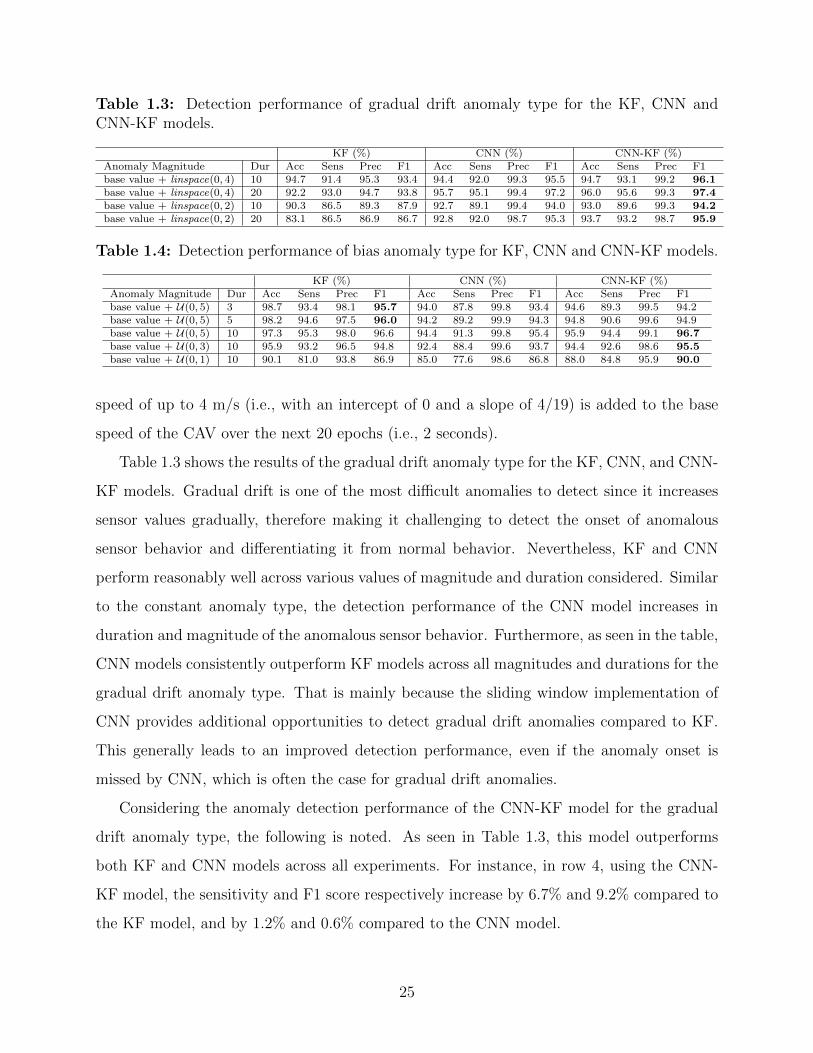
Table 1.3: Detection performance of gradual drift anomaly type for the KF, CNN andCNN-KF models.
KF (%) CNN (%) CNN-KF (%)Anomaly Magnitude Dur Acc Sens Prec F1 Acc Sens Prec F1 Acc Sens Prec F1base value + linspace(0, 4) 10 94.7 91.4 95.3 93.4 94.4 92.0 99.3 95.5 94.7 93.1 99.2 96.1base value + linspace(0, 4) 20 92.2 93.0 94.7 93.8 95.7 95.1 99.4 97.2 96.0 95.6 99.3 97.4base value + linspace(0, 2) 10 90.3 86.5 89.3 87.9 92.7 89.1 99.4 94.0 93.0 89.6 99.3 94.2base value + linspace(0, 2) 20 83.1 86.5 86.9 86.7 92.8 92.0 98.7 95.3 93.7 93.2 98.7 95.9
Table 1.4: Detection performance of bias anomaly type for KF, CNN and CNN-KF models.
KF (%) CNN (%) CNN-KF (%)Anomaly Magnitude Dur Acc Sens Prec F1 Acc Sens Prec F1 Acc Sens Prec F1base value + U(0, 5) 3 98.7 93.4 98.1 95.7 94.0 87.8 99.8 93.4 94.6 89.3 99.5 94.2base value + U(0, 5) 5 98.2 94.6 97.5 96.0 94.2 89.2 99.9 94.3 94.8 90.6 99.6 94.9base value + U(0, 5) 10 97.3 95.3 98.0 96.6 94.4 91.3 99.8 95.4 95.9 94.4 99.1 96.7base value + U(0, 3) 10 95.9 93.2 96.5 94.8 92.4 88.4 99.6 93.7 94.4 92.6 98.6 95.5base value + U(0, 1) 10 90.1 81.0 93.8 86.9 85.0 77.6 98.6 86.8 88.0 84.8 95.9 90.0
speed of up to 4 m/s (i.e., with an intercept of 0 and a slope of 4/19) is added to the base
speed of the CAV over the next 20 epochs (i.e., 2 seconds).
Table 1.3 shows the results of the gradual drift anomaly type for the KF, CNN, and CNN-
KF models. Gradual drift is one of the most difficult anomalies to detect since it increases
sensor values gradually, therefore making it challenging to detect the onset of anomalous
sensor behavior and differentiating it from normal behavior. Nevertheless, KF and CNN
perform reasonably well across various values of magnitude and duration considered. Similar
to the constant anomaly type, the detection performance of the CNN model increases in
duration and magnitude of the anomalous sensor behavior. Furthermore, as seen in the table,
CNN models consistently outperform KF models across all magnitudes and durations for the
gradual drift anomaly type. That is mainly because the sliding window implementation of
CNN provides additional opportunities to detect gradual drift anomalies compared to KF.
This generally leads to an improved detection performance, even if the anomaly onset is
missed by CNN, which is often the case for gradual drift anomalies.
Considering the anomaly detection performance of the CNN-KF model for the gradual
drift anomaly type, the following is noted. As seen in Table 1.3, this model outperforms
both KF and CNN models across all experiments. For instance, in row 4, using the CNN-
KF model, the sensitivity and F1 score respectively increase by 6.7% and 9.2% compared to
the KF model, and by 1.2% and 0.6% compared to the CNN model.
25
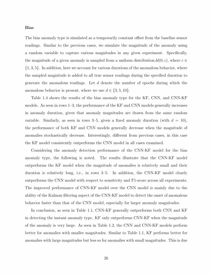
Bias
The bias anomaly type is simulated as a temporarily constant offset from the baseline sensor
readings. Similar to the previous cases, we simulate the magnitude of the anomaly using
a random variable to capture various magnitudes in any given experiment. Specifically,
the magnitude of a given anomaly is sampled from a uniform distribution U(0, c), where c ∈
{1, 3, 5}. In addition, here we account for various durations of the anomalous behavior, where
the sampled magnitude is added to all true sensor readings during the specified duration to
generate the anomalous readings. Let d denote the number of epochs during which the
anomalous behavior is present, where we use d ∈ {3, 5, 10}.
Table 1.4 shows the results of the bias anomaly type for the KF, CNN, and CNN-KF
models. As seen in rows 1–3, the performance of the KF and CNN models generally increases
in anomaly duration, given that anomaly magnitudes are drawn from the same random
variable. Similarly, as seen in rows 3–5, given a fixed anomaly duration (with d = 10),
the performance of both KF and CNN models generally decrease when the magnitude of
anomalies stochastically decrease. Interestingly, different from previous cases, in this case
the KF model consistently outperforms the CNN model in all cases examined.
Considering the anomaly detection performance of the CNN-KF model for the bias
anomaly type, the following is noted. The results illustrate that the CNN-KF model
outperforms the KF model when the magnitude of anomalies is relatively small and their
duration is relatively long, i.e., in rows 3–5. In addition, the CNN-KF model clearly
outperforms the CNN model with respect to sensitivity and F1-score across all experiments.
The improved performance of CNN-KF model over the CNN model is mainly due to the
ability of the Kalman filtering aspect of the CNN-KF model to detect the onset of anomalous
behavior faster than that of the CNN model, especially for larger anomaly magnitudes.
In conclusion, as seen in Table 1.1, CNN-KF generally outperforms both CNN and KF
in detecting the instant anomaly type. KF only outperforms CNN-KF when the magnitude
of the anomaly is very large. As seen in Table 1.2, the CNN and CNN-KF models perform
better for anomalies with smaller magnitudes. Similar to Table 1.1, KF performs better for
anomalies with large magnitudes but less so for anomalies with small magnitudes. This is due
26

to the fact that when the anomalies are small enough, they fall into the gating region of the
KF model; therefore, they cannot be detected by the chi-square test. Also, as seen in Table
1.3, the CNN-KF model outperforms both KF and CNN models across all magnitudes and
durations considered for the gradual drift anomaly type. This is mainly because CNN-KF
combines the strength of CNN where the sliding window implementation provides additional
opportunities for detection and the ability of KF in detecting the first few epochs of these
anomalies. Lastly, as seen in Table 1.4 for the bias anomaly type, consistent with the results
in Tables 1.1–1.3, the CNN-KF models perform well for anomalies with small magnitudes
and long duration whereas KF performs better for anomalies with large magnitudes and a
small duration.
1.4.2 Models Under Mixed Anomaly Types
In this section we investigate the performance of the models when applied in detection and
identification of various types of anomalies as opposed to the single anomaly types considered
in Section 1.4.1. First, we investigate the generalizability of the models presented in Section
1.4.1 with respect to unseen anomaly types to motivate the need to develop CNN-based
models under mixed anomaly types. Next we develop new models, trained and tested in the
presence of all four anomaly types, where the simulation is run multiple times to provide
confidence intervals (CIs). Specifically, we present the mean performance along with the 95%
CIs, and perform statistical tests to establish whether or not the observed improvements
across models are significant. In addition, we analyze the effect of the rate at which anoma-
lous sensor values may occur (at α = 5% and α = 1%) on the performance of the models.
As seen in Section 1.4.1, CNN and CNN-KF models generally outperform KF models.
However, note that in contrast to CNN models, KF models do not require much effort for
training and they generalize well; only parameters γ and M need to be calibrated for KF
models. Additionally, as we will demonstrate in this section, for CNN models to generalize
well and correctly classify previously unseen observations, they require to be trained on
representative training sets. However, in practice, CAV anomaly detection systems may
encounter various instances of anomalies for which the models are not explicitly trained.
This is particularly important for CAVs since these vehicles will be faced with numerous
27
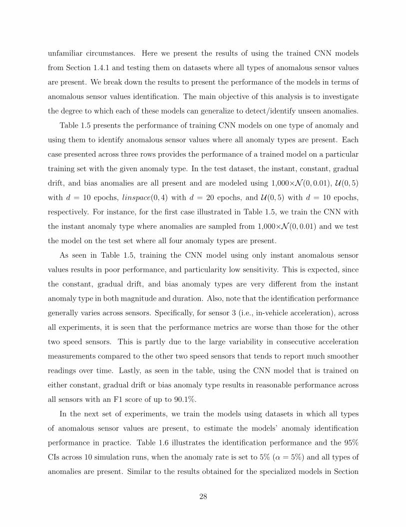
unfamiliar circumstances. Here we present the results of using the trained CNN models
from Section 1.4.1 and testing them on datasets where all types of anomalous sensor values
are present. We break down the results to present the performance of the models in terms of
anomalous sensor values identification. The main objective of this analysis is to investigate
the degree to which each of these models can generalize to detect/identify unseen anomalies.
Table 1.5 presents the performance of training CNN models on one type of anomaly and
using them to identify anomalous sensor values where all anomaly types are present. Each
case presented across three rows provides the performance of a trained model on a particular
training set with the given anomaly type. In the test dataset, the instant, constant, gradual
drift, and bias anomalies are all present and are modeled using 1,000×N (0, 0.01), U(0, 5)
with d = 10 epochs, linspace(0, 4) with d = 20 epochs, and U(0, 5) with d = 10 epochs,
respectively. For instance, for the first case illustrated in Table 1.5, we train the CNN with
the instant anomaly type where anomalies are sampled from 1,000×N (0, 0.01) and we test
the model on the test set where all four anomaly types are present.
As seen in Table 1.5, training the CNN model using only instant anomalous sensor
values results in poor performance, and particularity low sensitivity. This is expected, since
the constant, gradual drift, and bias anomaly types are very different from the instant
anomaly type in both magnitude and duration. Also, note that the identification performance
generally varies across sensors. Specifically, for sensor 3 (i.e., in-vehicle acceleration), across
all experiments, it is seen that the performance metrics are worse than those for the other
two speed sensors. This is partly due to the large variability in consecutive acceleration
measurements compared to the other two speed sensors that tends to report much smoother
readings over time. Lastly, as seen in the table, using the CNN model that is trained on
either constant, gradual drift or bias anomaly type results in reasonable performance across
all sensors with an F1 score of up to 90.1%.
In the next set of experiments, we train the models using datasets in which all types
of anomalous sensor values are present, to estimate the models’ anomaly identification
performance in practice. Table 1.6 illustrates the identification performance and the 95%
CIs across 10 simulation runs, when the anomaly rate is set to 5% (α = 5%) and all types of
anomalies are present. Similar to the results obtained for the specialized models in Section
28
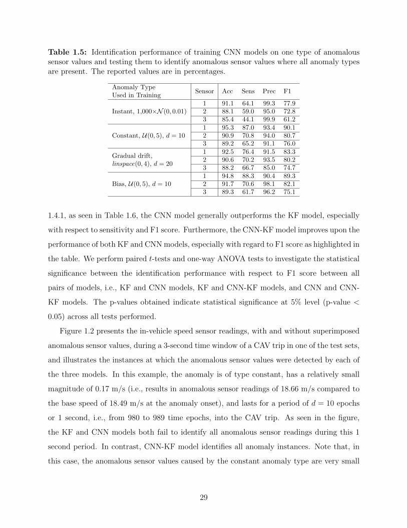
Table 1.5: Identification performance of training CNN models on one type of anomaloussensor values and testing them to identify anomalous sensor values where all anomaly typesare present. The reported values are in percentages.
Anomaly TypeUsed in Training
Sensor Acc Sens Prec F1
Instant, 1,000×N (0, 0.01)1 91.1 64.1 99.3 77.92 88.1 59.0 95.0 72.83 85.4 44.1 99.9 61.2
Constant, U(0, 5), d = 101 95.3 87.0 93.4 90.12 90.9 70.8 94.0 80.73 89.2 65.2 91.1 76.0
Gradual drift,linspace(0, 4), d = 20
1 92.5 76.4 91.5 83.32 90.6 70.2 93.5 80.23 88.2 66.7 85.0 74.7
Bias, U(0, 5), d = 101 94.8 88.3 90.4 89.32 91.7 70.6 98.1 82.13 89.3 61.7 96.2 75.1
1.4.1, as seen in Table 1.6, the CNN model generally outperforms the KF model, especially
with respect to sensitivity and F1 score. Furthermore, the CNN-KF model improves upon the
performance of both KF and CNN models, especially with regard to F1 score as highlighted in
the table. We perform paired t-tests and one-way ANOVA tests to investigate the statistical
significance between the identification performance with respect to F1 score between all
pairs of models, i.e., KF and CNN models, KF and CNN-KF models, and CNN and CNN-
KF models. The p-values obtained indicate statistical significance at 5% level (p-value <
0.05) across all tests performed.
Figure 1.2 presents the in-vehicle speed sensor readings, with and without superimposed
anomalous sensor values, during a 3-second time window of a CAV trip in one of the test sets,
and illustrates the instances at which the anomalous sensor values were detected by each of
the three models. In this example, the anomaly is of type constant, has a relatively small
magnitude of 0.17 m/s (i.e., results in anomalous sensor readings of 18.66 m/s compared to
the base speed of 18.49 m/s at the anomaly onset), and lasts for a period of d = 10 epochs
or 1 second, i.e., from 980 to 989 time epochs, into the CAV trip. As seen in the figure,
the KF and CNN models both fail to identify all anomalous sensor readings during this 1
second period. In contrast, CNN-KF model identifies all anomaly instances. Note that, in
this case, the anomalous sensor values caused by the constant anomaly type are very small
29
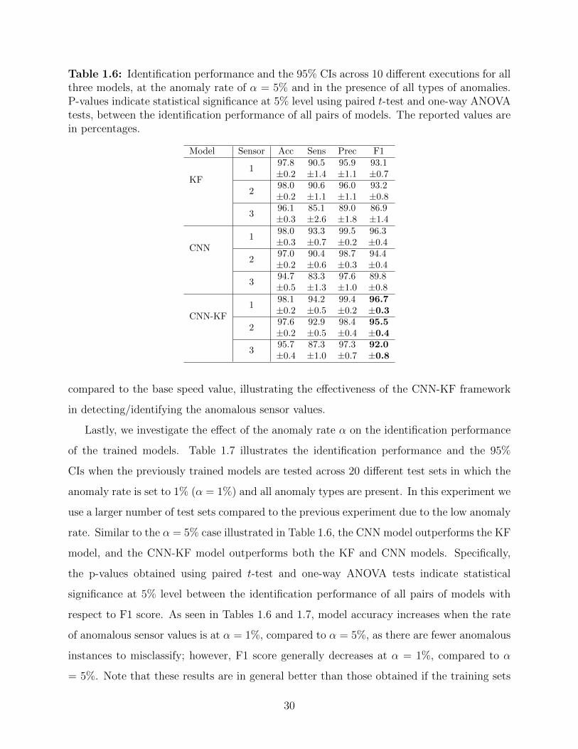
Table 1.6: Identification performance and the 95% CIs across 10 different executions for allthree models, at the anomaly rate of α = 5% and in the presence of all types of anomalies.P-values indicate statistical significance at 5% level using paired t-test and one-way ANOVAtests, between the identification performance of all pairs of models. The reported values arein percentages.
Model Sensor Acc Sens Prec F1
KF1
97.8±0.2
90.5±1.4
95.9±1.1
93.1±0.7
298.0±0.2
90.6±1.1
96.0±1.1
93.2±0.8
396.1±0.3
85.1±2.6
89.0±1.8
86.9±1.4
CNN1
98.0±0.3
93.3±0.7
99.5±0.2
96.3±0.4
297.0±0.2
90.4±0.6
98.7±0.3
94.4±0.4
394.7±0.5
83.3±1.3
97.6±1.0
89.8±0.8
CNN-KF1
98.1±0.2
94.2±0.5
99.4±0.2
96.7±0.3
297.6±0.2
92.9±0.5
98.4±0.4
95.5±0.4
395.7±0.4
87.3±1.0
97.3±0.7
92.0±0.8
compared to the base speed value, illustrating the effectiveness of the CNN-KF framework
in detecting/identifying the anomalous sensor values.
Lastly, we investigate the effect of the anomaly rate α on the identification performance
of the trained models. Table 1.7 illustrates the identification performance and the 95%
CIs when the previously trained models are tested across 20 different test sets in which the
anomaly rate is set to 1% (α = 1%) and all anomaly types are present. In this experiment we
use a larger number of test sets compared to the previous experiment due to the low anomaly
rate. Similar to the α = 5% case illustrated in Table 1.6, the CNN model outperforms the KF
model, and the CNN-KF model outperforms both the KF and CNN models. Specifically,
the p-values obtained using paired t-test and one-way ANOVA tests indicate statistical
significance at 5% level between the identification performance of all pairs of models with
respect to F1 score. As seen in Tables 1.6 and 1.7, model accuracy increases when the rate
of anomalous sensor values is at α = 1%, compared to α = 5%, as there are fewer anomalous
instances to misclassify; however, F1 score generally decreases at α = 1%, compared to α
= 5%. Note that these results are in general better than those obtained if the training sets
30
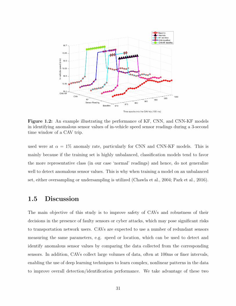
Figure 1.2: An example illustrating the performance of KF, CNN, and CNN-KF modelsin identifying anomalous sensor values of in-vehicle speed sensor readings during a 3-secondtime window of a CAV trip.
used were at α = 1% anomaly rate, particularly for CNN and CNN-KF models. This is
mainly because if the training set is highly unbalanced, classification models tend to favor
the more representative class (in our case ‘normal’ readings) and hence, do not generalize
well to detect anomalous sensor values. This is why when training a model on an unbalanced
set, either oversampling or undersampling is utilized (Chawla et al., 2004; Park et al., 2016).
1.5 Discussion
The main objective of this study is to improve safety of CAVs and robustness of their
decisions in the presence of faulty sensors or cyber attacks, which may pose significant risks
to transportation network users. CAVs are expected to use a number of redundant sensors
measuring the same parameters, e.g. speed or location, which can be used to detect and
identify anomalous sensor values by comparing the data collected from the corresponding
sensors. In addition, CAVs collect large volumes of data, often at 100ms or finer intervals,
enabling the use of deep learning techniques to learn complex, nonlinear patterns in the data
to improve overall detection/identification performance. We take advantage of these two
31
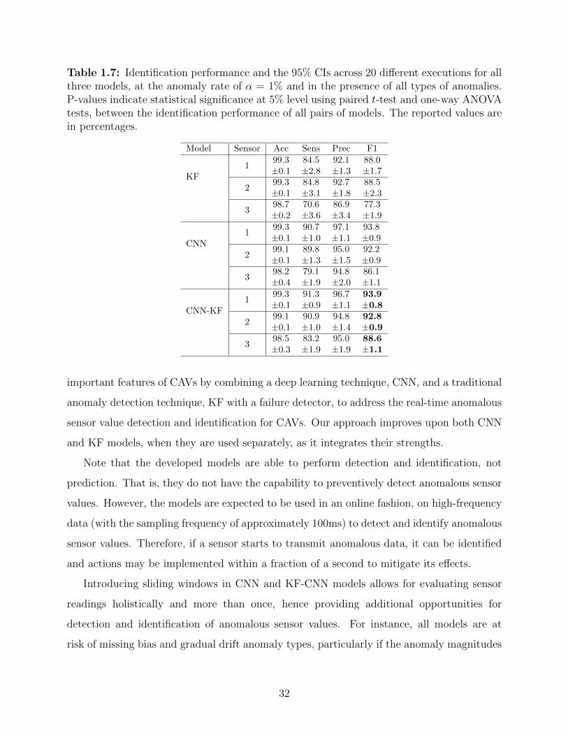
Table 1.7: Identification performance and the 95% CIs across 20 different executions for allthree models, at the anomaly rate of α = 1% and in the presence of all types of anomalies.P-values indicate statistical significance at 5% level using paired t-test and one-way ANOVAtests, between the identification performance of all pairs of models. The reported values arein percentages.
Model Sensor Acc Sens Prec F1
KF1
99.3±0.1
84.5±2.8
92.1±1.3
88.0±1.7
299.3±0.1
84.8±3.1
92.7±1.8
88.5±2.3
398.7±0.2
70.6±3.6
86.9±3.4
77.3±1.9
CNN1
99.3±0.1
90.7±1.0
97.1±1.1
93.8±0.9
299.1±0.1
89.8±1.3
95.0±1.5
92.2±0.9
398.2±0.4
79.1±1.9
94.8±2.0
86.1±1.1
CNN-KF1
99.3±0.1
91.3±0.9
96.7±1.1
93.9±0.8
299.1±0.1
90.9±1.0
94.8±1.4
92.8±0.9
398.5±0.3
83.2±1.9
95.0±1.9
88.6±1.1
important features of CAVs by combining a deep learning technique, CNN, and a traditional
anomaly detection technique, KF with a failure detector, to address the real-time anomalous
sensor value detection and identification for CAVs. Our approach improves upon both CNN
and KF models, when they are used separately, as it integrates their strengths.
Note that the developed models are able to perform detection and identification, not
prediction. That is, they do not have the capability to preventively detect anomalous sensor
values. However, the models are expected to be used in an online fashion, on high-frequency
data (with the sampling frequency of approximately 100ms) to detect and identify anomalous
sensor values. Therefore, if a sensor starts to transmit anomalous data, it can be identified
and actions may be implemented within a fraction of a second to mitigate its effects.
Introducing sliding windows in CNN and KF-CNN models allows for evaluating sensor
readings holistically and more than once, hence providing additional opportunities for
detection and identification of anomalous sensor values. For instance, all models are at
risk of missing bias and gradual drift anomaly types, particularly if the anomaly magnitudes
32
are small. However, in CNN and CNN-KF, even if the onset of anomaly is initially missed,
the anomaly is detected/identified after only a few time epochs, e.g., approximately in 300ms.
1.6 Conclusion and Future Work
The goal of this study is to develop an approach to detect/identify anomalous behaviors in
CAVs to improve their safety. Our results show that the use of deep learning models such as
CNN to detect/identify anomalous sensor values in CAV systems in real-time is a viable path
and it can improve upon the well-established methods such as Kalman filtering with failure
detectors. In addition, our results show that because of the inherent differences between
CNN and KF, combining these approaches can build upon their individual strengths and
hence result in an improved performance. More specifically, we show that by using a CNN-
empowered KF on raw sensor data, it is possible to detect and identify anomalous sensor
values in real-time with high accuracy, sensitivity, precision, and F1 score. This research
contributes to the field of ITS safety as a whole since the success of ITS operations is
heavily dependent on the safe operation of all its respective elements. In addition, CAV
manufacturers and policy-makers may benefit from the observations in this study with
regards to the value of having redundant information for a specific parameter such as the
speed of a vehicle. As a result, more redundant sensors and information gathering devices
may be implemented and considered in CAVs to increase their resiliency against anomalous
sensor values. It is also expected that the CNN-KF framework presented in this study will
be applied to various other sources of information in CAVs to increase their safety.
The study is subject to limitations. First, the anomalous sensor values used in the
experiments, consistent with previous studies in the literature, are simulated, mainly because
this type of data are not yet readily available. In addition, due to paucity of data on
connected vehicles, the experiments are limited to on-board sensors. Although the framework
is generic and can address anomaly detection/identification regardless of the data source,
additional testing is needed as real data becomes readily available. To that end, it should
be noted that the reported performance of the proposed CNN-based methods are only valid
33

for those attack types whose effects can be reflected by the four anomaly types considered
in this study.
Furthermore, in this study, we assume the onset of anomalous values in sensors, due to
either attacks or faults, occur independently. Although we do not explicitly train models on
datasets containing interdependent sensor failures or systemic cyber attacks on a vehicle’s
sensors, the framework is expected to still be able to detect such faults/attacks. To improve
model performance under such scenarios, however, additional training using such data is
required. Indeed, it is envisioned that real-world data would be available in the near future
as a result of various ongoing pilot studies (Michigan, Wyoming, New York City, and Tampa)
as well as the introduction of CAVs into society by companies such as Waymo, Uber, Audi,
and Tesla.
In future work, it may be useful to distinguish between anomalous and malicious
information, since this will influence the action taken to mitigate their effects. Also, it
may be beneficial to also identify the type of anomaly occurring. This, in turn, will enable
the development of certain real-time actions to minimize the impact of cyber attacks and/or
faulty sensors, therefore contributing to the development of effective counter-measures.
34
Chapter 2
Optimal Switching Policy Between
Driving Entities in Semi-Autonomous
Vehicles
35
Disclosure: This chapter is based on a paper submitted by van Wyk et al. (2019) to
Transportation Research Part C: Emerging Technologies.
van Wyk, F., Khojandi, A. and Masoud, N., 2019. Optimal Switching Policy Between
Driving Entities in Semi-Autonomous Vehicles. Transportation Research Part C: Emerging
Technologies.
My contributions to this paper include: (i) the development of the problem, (ii)
reviewing the appropriate literature, (iii) the identification of study objectives, (iv) design
and conducting of the numerical experiments, (v) majority of the writing responsibilities of
the manuscript.
Abstract
In the future, autonomous vehicles are expected to safely move people and cargo around.
However, as of now, automated entities do not necessarily outperform human drivers under
all circumstances, particularly under certain road and environmental factors such as bright
light, heavy rain, poor quality of road and traffic signs, etc. Therefore, in certain conditions
it is safer for the driver to take over the control of the vehicle. However, switching control
back and forth between the human driver and the automated driving entity may itself pose
a short-term, elevated risk, particularly because of the out of the loop (OOTL) issue for
humans. In this study, we develop a mathematical framework to determine the optimal
driving-entity switching policy between the automated driving entity and the human driver.
Specifically, we develop a Markov decision process (MDP) model to prescribe the entity
in charge to minimize the expected safety cost of a trip, considering the dynamic changes
of the road/environment during the trip. In addition, we develop a partially observable
Markov decision process (POMDP) model to accommodate the fact that the risk posed by
the immediate road/environment may only be partially observed. We conduct extensive
numerical experiments and thorough sensitivity and robustness analyses, where we also
compare the expected safety cost of trips under the optimal and single driving entity policies.
In addition, we quantify the risks associated with the policies, as well as the impact of miss-
estimating road/environment condition risk level by the driving entities, and provide insights.
36
2.1 Introduction
It is expected that connected and autonomous vehicles (CAVs) will increase road safety,
reduce travel time, improve comfort, improve fuel efficiency and decrease fatal accidents by
as much as 40% in the future (Fagnant and Kockelman, 2015; Guler et al., 2014). However,
before transportation systems are fully connected and automated, there will be a transition
period where the driver is required to retake control of the vehicle from the autonomous
system at certain times under various circumstances (Campbell et al., 2018).
The Society of Automotive Engineers (SAE) has identified 6 levels of autonomy (levels
0 through 5) that reflect the nature of interactions between an automated vehicle and the
driving environment as well as the degree of driver involvement (SAE, 2016). Level 0 refers
to the driver performing all dynamic driving tasks. Level 1 automation entails assisted
automation where advanced driver assistance systems (ADAS) perform steering, acceleration
or deceleration. Level 2 automation is present if one or more assisted automation tasks are
performed by the autonomous system where the driver is responsible for the monitoring of
the driving environment and ultimately the control of the vehicle.
In level 3 and higher automation levels, the autonomous system continuously monitors the
environment using sensors, cameras, radars, and a global positioning system (GPS) feeding
information to the control software. A typical autonomous system in a vehicle acquires
information, analyzes the information, and then implements the optimal action/decision.
Specifically, in level 3 automation the vehicle can autonomously drive for the most part;
however, drivers are encouraged to monitor the driving environment at all times and are
expected to take over the control when requested by the autonomous system in certain
situations. In level 4 automation, the autonomous driving system is able to perform all
driving tasks under certain conditions and the driver has the option to control the vehicle.
In level 5 automation, the autonomous driving system is able to perform all driving tasks in
all conditions.
It is often argued that fully autonomous vehicles (level 5) will be able to outperform
human drivers and hence relying on autonomous driving technology will improve safety;
however, many experts argue that there is still a long way ahead. First, for the foreseeable
37
future, the presence of human drivers will be required in all autonomous vehicles due to
technology limitations and certain legislative factors (Goodrich and Boer, 2000; Parasuraman
and Manzey, 2010; Kyriakidis et al., 2015). In addition, autonomous vehicles consist of
highly complex electronic systems interacting with hardware and the environment making
them vulnerable to certain threats that may pose risk to people in the vehicle as well as
pedestrians and other road users (Petit and Shladover, 2015). As evident by the recent
crash records for vehicles with varying degrees of autonomy, one major threat is extreme
road and immediate environmental conditions which may affect the integrity and reliability
of autonomous technologies. Road and environmental factors such as bright light, heavy rain,
snow, or fog and poor road and traffic signs quality may affect the ability of autonomous
systems to function properly (Tesla, 2017). For instance, in 2016, a fatal accident occurred
when a level 2 autonomous vehicle was in control and collided with a tractor-trailer that was
making a turn. The autonomous system sensors failed to recognize the difference between
the truck and bright sky, causing the collision. In 2017, another vehicle with autonomous
capabilities crashed into a road construction barrier after it failed to recognize the roadway
and merge into another lane (Lambert, 2017). This occurred as a result of various factors
including poorly implemented road construction and failure in the ability of the autonomous
system to recognize the upcoming wall.
Overall, implementing intermediate levels of automation, i.e., levels 2 through 4, is seen
as the next phase in the mass adoption of autonomous driving technologies. Indeed, over
the past decade, there has been a rapid increase in the development of vehicles equipped
with advanced driver assistance systems. Vehicle manufacturers such as Tesla, Toyota,
BMW, Nissan, Audi, General Motors, and Volvo have equipped vehicles with autonomous
technologies such as autonomous emergency braking (AEB), adaptive cruise control (ACC),
lane keeping assist (LKA), and automatic parking constituting various levels of autonomy
as specified by the SAE (SAE, 2014; Lu and de Winter, 2015). Manufacturers like Audi and
Tesla already have implemented level 3 automation in recently released models. In levels 2
through 4, it is envisioned that the human driver has the option to take over the control of
vehicle. Therefore, if high risk circumstances are anticipated, there is a possibility to pass
the control to the human driver in a timely manner to reduce the overall safety risk.
38
Switching control back and forth between the human driver and the autonomous driving
entity to maximize safety may not be straightforward as every such switch can itself pose
a short-term, elevated risk. With intermediate levels of automation, drivers are expected to
engage in various activities (e.g., smartphone and tablet use) while the autonomous system is
in control, but will be required to take control of the vehicle at certain times or based on feed-
back from the system. Hence, one of the factors that makes the transition of control between
the two driving entities challenging is the potentially long transition time for transferring the
control from the autonomous system to the driver due to a phenomenon known as the ‘out-of-
the-loop’ (OOTL) problem, caused by the disengagement of the driver from the environment.
After being disengaged from the driving environment during the period where the
autonomous system is in control, drivers are naturally expected to have higher reaction
times (RT). Even in levels 0-2 autonomy, drivers need time to recognize the occurrence of
an out-of-the-ordinary event, decide on an appropriate action, and act upon this decision.
Research shows that RT can vary widely, ranging from 0.7 seconds when an event is expected,
to 1.5 seconds when it is not (e.g., sudden braking from the lead vehicle) (Green, 2000). Even
when drivers have full control of the car during the entire trip, their “expectation” can affect
reaction times by as much as a factor of 2 (Green, 2000). With the promise of freedom
from constant engagement with the driving environment, level 3 autonomy can have more
dramatic affects on driver reaction times, increasing the time it takes to regain the driver’s
attention to 3 to 7 seconds, even with visual and verbal warnings, according to a study by
Audi (Davies, 2015).
To that end, OOTL problems arise when the driver has to re-take control of the vehicle
from the automated system after engagement with secondary tasks over a period of time.
De Winter et al. (2014) showed that the workload of drivers and situation awareness are
vastly different for driving with assisted autonomy, i.e., levels 1 and 2 autonomy, compared to
highly automated driving (HAD), i.e., level 3 and higher autonomy. More specifically, mental
workload and situation awareness generally decrease with increasing levels of automation
and the brake reaction time of drivers increase for automated systems compared to manual
driving (Young and Stanton, 2007; Kaber and Endsley, 2004; Merat et al., 2014b). Other
studies have investigated the effect of the transition of control authority on the way drivers
39
reclaim control of the vehicle, also known as ‘take-over quality’ (Miller et al., 2015; Merat
et al., 2014a; Strand et al., 2014; Koo et al., 2016). In general, these studies conclude that for
higher levels of autonomy drivers need more time to re-obtain full control over the vehicle. In
addition, for short warning times it was found that the take-over quality drastically decreases,
therefore illustrating that accidents and near-accidents are likely to occur when the driver
resumes control. In poor quality take-overs, it was found that the transition process may
result in situations where drivers accidentally swerve, brake harshly, or perform sudden lane
changes (Eriksson and Stanton, 2017). Automation may therefore often reduce the workload
during non-dangerous driving conditions, but sudden control changes may be detrimental to
driving safety (Rudin-Brown and Parker, 2004; Koo et al., 2016).
Therefore, it is necessary to balance the short-term risks of switching entity and the
long-term risks of continuing with the entity in charge, given the dynamic changes of
road/environment. In this study, we develop a mathematical framework to optimally
plan a trip by dynamically switching the control between the human driver and self-
driving technology to provide the safest driving profile. Specifically, first we develop a
Markov decision process (MDP) model to prescribe the driving entity in charge and the
timing of transfers as a function of the road condition and environmental changes. The
objective is to determine the optimal driving-entity switching policy to minimize the total
expected discounted cost of possible accidents, considering the dynamic changes of the
road/environment during the trip. This model is relatively compact and provides an
opportunity to easily investigate the impact of switching driving entities and draw insights
about the risks involved.
However, note that in this MDP model, we assume the road/environment condition is
completely observable, i.e., both driving entities can accurately assess the road/environment
condition during the trip and determine its exact safety risk level. Clearly, this implies that
the vehicle is equipped with an algorithm that can accurately evaluate the road/environment
condition and determine its exact safety risk level. Given the advances in machine learning
and image processing, this may soon become a reality. However, most existing algorithms,
as well as human drivers, are not always one hundred percent accurate in their evaluations.
Hence, we also relax this assumption and develop a partially observable Markov decision
40
process (POMDP) model, in which the risk posed by the road/environment condition is
only ‘partially’ observed and is prone to erroneous estimations.
The chapter is organized as follows. We formulate the model under complete and partial
information in Section 2.2. In Section 2.3, we provide extensive computational studies to
illustrate the benefits of switching control authority and investigate the model sensitivity
and robustness with respect to those model parameters that are most difficult to calibrate.
Lastly, we conclude in Section 2.4 and provide insights.
2.2 Model Formulation
In this section, we formulate models under different conditions to determine the optimal
driving entity. First, we assume the model has complete information regarding the state of
the system in which case we formulate a Markov decision process (MDP). That is, we assume
the model has perfect information regarding the location, environment, and driving entity in
charge. Next, we assume partial information regarding the state of the environment where
it is assumed that the environmental risk is obtained through a separate algorithm. In this
case, we formulate the system as a partially observable Markov decision process (POMDP).
2.2.1 Under Full Information
In this section, we develop an MDP model to optimally plan a trip by dynamically switching
the control between the human driver and the autonomous driving entity to minimize the
total expected cost of accidents throughout a trip. In this study, three types of consequences
for a motor vehicle crash are considered, namely, vehicle damage, bodily injury, and fatality,
to each of which a cost is assigned. Every time period (e.g., every second), a decision is
made as to whether the human driver or the car needs to take control of the vehicle. It is
assumed that the car can immediately take over the vehicle control from the human driver
once a decision for this switch is made. However, dependent on the driver’s reaction time,
it may take up to a few seconds for the human driver to take over the vehicle control if such
a decision is made.
41

Let st = (µ, φ, d) ∈ S denote the state of the process at time t ≤ T , where T <∞ denotes
the length of the time horizon. Let the vector µ = [`, ξ] denote the location-environment
vector. Specifically, the vector ` ∈ L denotes the location of the vehicle, where the set
L includes the location of the origin and destination, denoted by `O and `D, respectively,
and all other locations in the path between the origin and the destination. In addition, the
vector ξ ∈ Ξ denotes the state of the road/environment, e.g., weather, number of pedestrians,
quality of the road segment, etc. Furthermore, we let φ ∈ {I, C} denote the entity in charge
of driving the vehicle, where I refers to the ‘individual’ and C refers to the ‘car.’ Lastly, we
let d denote the time to the next scheduled switch in the driving entity from the car to the
individual, if it is previously scheduled, and assign to it the value -1, otherwise.
We discretize time into periods, e.g., seconds. At the beginning of every time period, a
decision is made as to whether the human driver or the car needs to take control of the vehicle.
Let a ∈ A = {I, C} denote the action taken in each decision epoch. Recall that although
the car can immediately take over the vehicle control from the individual, dependent on the
individual’s reaction time, it may take up to a few seconds for the individual to take over the
vehicle control. Let k > 0 denote the length of time it takes for the driver to take over the
vehicle control from the car once a decision is made to switch the control. Also, we let cA
denote the cost of alerting the individual to take over the control, and cP denote the penalty
of foregoing a previously made decision to hand over the control to the individual before it
is implemented. These costs penalize unnecessary alerts that may cause alarm fatigue in the
long run.
Let pφ(µ) denote the probability of accident for the driving entity φ at location-
environment µ, and let q0(φ,µ), q1(φ,µ), and q2(φ,µ) denote the conditional probability
of damage, injury and fatality, given an accident occurs for driving entity φ at location-
environment µ, respectively. Similarly, let ζφ(µ) denote the probability of accident at
location-environment µ as a result of a switch of the vehicle control to entity φ, and let ρ0(µ),
ρ1(µ), and ρ2(µ) denote the conditional probability of damage, injury and fatality, given an
accident occurs at location-environment µ following the switch in driving entity, respectively.
Let c0, c1, and c2 denote the cost of damage, injury and fatality of an accident,
respectively. Consequently, let β(φ,µ) denote the expected immediate cost of accident for
42
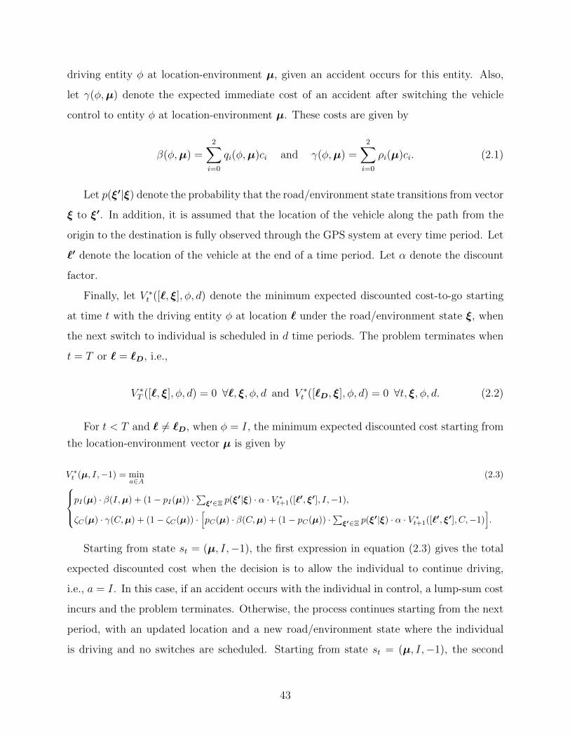
driving entity φ at location-environment µ, given an accident occurs for this entity. Also,
let γ(φ,µ) denote the expected immediate cost of an accident after switching the vehicle
control to entity φ at location-environment µ. These costs are given by
β(φ,µ) =2∑i=0
qi(φ,µ)ci and γ(φ,µ) =2∑i=0
ρi(µ)ci. (2.1)
Let p(ξ′|ξ) denote the probability that the road/environment state transitions from vector
ξ to ξ′. In addition, it is assumed that the location of the vehicle along the path from the
origin to the destination is fully observed through the GPS system at every time period. Let
`′ denote the location of the vehicle at the end of a time period. Let α denote the discount
factor.
Finally, let V ∗t ([`, ξ], φ, d) denote the minimum expected discounted cost-to-go starting
at time t with the driving entity φ at location ` under the road/environment state ξ, when
the next switch to individual is scheduled in d time periods. The problem terminates when
t = T or ` = `D, i.e.,
V ∗T ([`, ξ], φ, d) = 0 ∀`, ξ, φ, d and V ∗t ([`D, ξ], φ, d) = 0 ∀t, ξ, φ, d. (2.2)
For t < T and ` 6= `D, when φ = I, the minimum expected discounted cost starting from
the location-environment vector µ is given by
V ∗t (µ, I,−1) = mina∈A
(2.3)pI(µ) · β(I,µ) + (1− pI(µ)) ·∑ξ′∈Ξ p(ξ
′|ξ) · α · V ∗t+1([`′, ξ′], I,−1),
ζC(µ) · γ(C,µ) + (1− ζC(µ)) ·[pC(µ) · β(C,µ) + (1− pC(µ)) ·
∑ξ′∈Ξ p(ξ
′|ξ) · α · V ∗t+1([`′, ξ′], C,−1)].
Starting from state st = (µ, I,−1), the first expression in equation (2.3) gives the total
expected discounted cost when the decision is to allow the individual to continue driving,
i.e., a = I. In this case, if an accident occurs with the individual in control, a lump-sum cost
incurs and the problem terminates. Otherwise, the process continues starting from the next
period, with an updated location and a new road/environment state where the individual
is driving and no switches are scheduled. Starting from state st = (µ, I,−1), the second
43
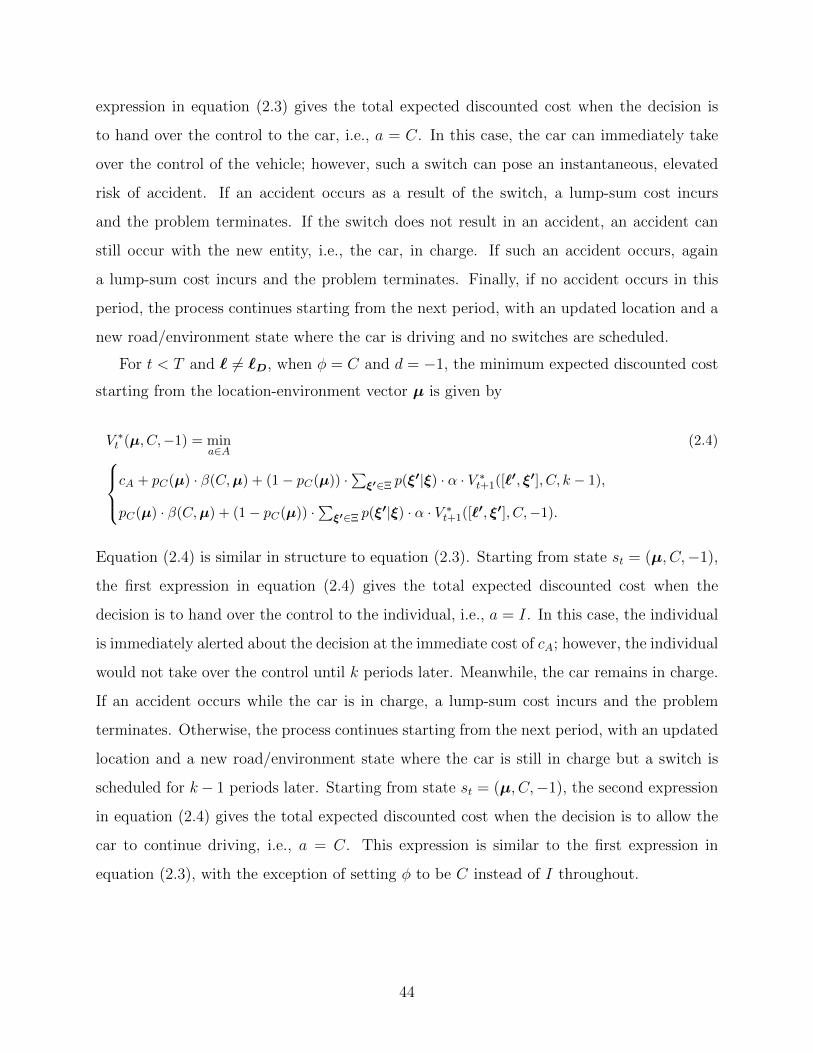
expression in equation (2.3) gives the total expected discounted cost when the decision is
to hand over the control to the car, i.e., a = C. In this case, the car can immediately take
over the control of the vehicle; however, such a switch can pose an instantaneous, elevated
risk of accident. If an accident occurs as a result of the switch, a lump-sum cost incurs
and the problem terminates. If the switch does not result in an accident, an accident can
still occur with the new entity, i.e., the car, in charge. If such an accident occurs, again
a lump-sum cost incurs and the problem terminates. Finally, if no accident occurs in this
period, the process continues starting from the next period, with an updated location and a
new road/environment state where the car is driving and no switches are scheduled.
For t < T and ` 6= `D, when φ = C and d = −1, the minimum expected discounted cost
starting from the location-environment vector µ is given by
V ∗t (µ, C,−1) = mina∈A
(2.4)cA + pC(µ) · β(C,µ) + (1− pC(µ)) ·
∑ξ′∈Ξ p(ξ
′|ξ) · α · V ∗t+1([`′, ξ′], C, k − 1),
pC(µ) · β(C,µ) + (1− pC(µ)) ·∑ξ′∈Ξ p(ξ
′|ξ) · α · V ∗t+1([`′, ξ′], C,−1).
Equation (2.4) is similar in structure to equation (2.3). Starting from state st = (µ, C,−1),
the first expression in equation (2.4) gives the total expected discounted cost when the
decision is to hand over the control to the individual, i.e., a = I. In this case, the individual
is immediately alerted about the decision at the immediate cost of cA; however, the individual
would not take over the control until k periods later. Meanwhile, the car remains in charge.
If an accident occurs while the car is in charge, a lump-sum cost incurs and the problem
terminates. Otherwise, the process continues starting from the next period, with an updated
location and a new road/environment state where the car is still in charge but a switch is
scheduled for k− 1 periods later. Starting from state st = (µ, C,−1), the second expression
in equation (2.4) gives the total expected discounted cost when the decision is to allow the
car to continue driving, i.e., a = C. This expression is similar to the first expression in
equation (2.3), with the exception of setting φ to be C instead of I throughout.
44
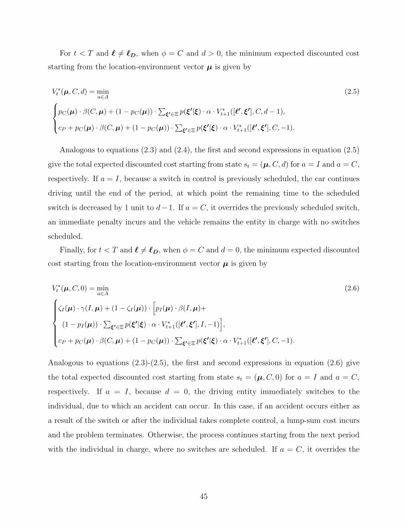
For t < T and ` 6= `D, when φ = C and d > 0, the minimum expected discounted cost
starting from the location-environment vector µ is given by
V ∗t (µ, C, d) = mina∈A
(2.5)pC(µ) · β(C,µ) + (1− pC(µ)) ·
∑ξ′∈Ξ p(ξ
′|ξ) · α · V ∗t+1([`′, ξ′], C, d− 1),
cP + pC(µ) · β(C,µ) + (1− pC(µ)) ·∑ξ′∈Ξ p(ξ
′|ξ) · α · V ∗t+1([`′, ξ′], C,−1).
Analogous to equations (2.3) and (2.4), the first and second expressions in equation (2.5)
give the total expected discounted cost starting from state st = (µ, C, d) for a = I and a = C,
respectively. If a = I, because a switch in control is previously scheduled, the car continues
driving until the end of the period, at which point the remaining time to the scheduled
switch is decreased by 1 unit to d−1. If a = C, it overrides the previously scheduled switch,
an immediate penalty incurs and the vehicle remains the entity in charge with no switches
scheduled.
Finally, for t < T and ` 6= `D, when φ = C and d = 0, the minimum expected discounted
cost starting from the location-environment vector µ is given by
V ∗t (µ, C, 0) = mina∈A
(2.6)ζI(µ) · γ(I,µ) + (1− ζI(µ)) ·
[pI(µ) · β(I,µ)+
(1− pI(µ)) ·∑ξ′∈Ξ p(ξ
′|ξ) · α · V ∗t+1([`′, ξ′], I,−1)],
cP + pC(µ) · β(C,µ) + (1− pC(µ)) ·∑ξ′∈Ξ p(ξ
′|ξ) · α · V ∗t+1([`′, ξ′], C,−1).
Analogous to equations (2.3)-(2.5), the first and second expressions in equation (2.6) give
the total expected discounted cost starting from state st = (µ, C, 0) for a = I and a = C,
respectively. If a = I, because d = 0, the driving entity immediately switches to the
individual, due to which an accident can occur. In this case, if an accident occurs either as
a result of the switch or after the individual takes complete control, a lump-sum cost incurs
and the problem terminates. Otherwise, the process continues starting from the next period
with the individual in charge, where no switches are scheduled. If a = C, it overrides the
45
previously scheduled switch and the same expression as the second expression in equation
(2.5) follows.
2.2.2 Under Partial Information
In this section, we assume that the state of the environment, ξ, is only partially observed.
That is, we assume the vehicle is equipped with an algorithm, e.g., a sequential image
classification algorithm, that can estimate the degree of risk in the environment. Clearly,
such an algorithm is subject to error and does not necessarily have 100% sensitivity or
specificity. Hence, we assume the information only partially informs the authority switching
decision making process.
We assume the set Ξ is countable, and let πt = [πξt (ξ1), πξt (ξ2), . . . , πξt (ξ|Ξ|)] denote the
belief state of the environment, where πξt (ξj) ≥ 0 is the probability that the vehicle is in
road/environment state ξj ∈ Ξ at time t and∑|Ξ|
j=1 πξt (ξj) = 1. At every time epoch, the
algorithm is used to observe the state of the environment, where the observation is later
incorporated to update the belief vector. Let oξt denote the observation made about the
state of the environment at time t.
Let zt = (`,π, φ, d) denote the state of the process, including the fully known information
and partially informed state of the environment, at time t ≤ T , where T < ∞ denotes the
length of the time horizon. Let W ∗t (`,π, φ, d) denote the minimum expected discounted cost-
to-go starting at time t, the driving entity φ in charge, at location ` under the environment
belief vector π, when the next switch to individual is scheduled in d time periods. Similar
to Section 2.2.1, the problem terminates when t = T or ` = `D, i.e.,
W ∗T (`,π, φ, d) = 0 ∀`,π, φ, d and W ∗
t (`D,π, φ, d) = 0 ∀t,π, φ, d. (2.7)
46
For t < T and ` 6= `D, when φ = I, the minimum expected discounted cost starting from
any location ` and environment belief vector π is given by
W ∗t (`,π, I,−1) = mina∈A
(2.8)
∑ξ∈Ξ π
ξt (ξ) · pI(µ) · β(I,µ)+∑
ξ∈Ξ πξt (ξ) · (1− pI(µ)) ·
∑ξ′∈Ξ
∑oξt+1∈Ξ
p(ξ′|ξ)p(oξt+1|ξ′) · α ·W ∗t+1(`′,π′, I,−1),∑ξ∈Ξ π
ξt (ξ) ·
[ζC(µ) · γ(C,µ) + (1− ζC(µ)) · pC(µ) · β(C,µ)
]+∑ξ∈Ξ π
ξt (ξ)·
(1− ζC(µ)) · (1− pC(µ)) ·∑ξ′∈Ξ
∑oξt+1∈Ξ
p(ξ′|ξ) · p(oξt+1|ξ′) · α ·W ∗t+1(`′,π′, C,−1),
where π′ = [πξt+1(ξ1), πξt+1(ξ2), . . . , πξt+1(ξ|Ξ|)] and
πξt+1(ξi) =p(oξt+1|ξi)
∑ξj∈Ξ p(ξi|ξj)π
ξt (ξj)∑
ξi∈Ξ p(oξt+1|ξi)
∑ξj∈Ξ p(ξi|ξj)π
ξt (ξj)
∀ξi ∈ Ξ. (2.9)
Equation (2.8) is analogous to equation (2.3) in Section 2.2.1, where the first and second
expressions in the equation give the total expected discounted cost when the decisions are to
allow the individual to continue driving, i.e., a = I, and to hand over the control to the car,
i.e., a = C, respectively. Similarly, analogous to equations (2.4), (2.5), and (2.6) in Section
2.2.1, Bellman equations can be written for t < T and ` 6= `D, when φ = C and d = −1,
d > 0, and d = 0, respectively.
To solve the developed POMDP model, we use the asynchronous advantage actor critic
(A3C) algorithm (Mnih et al., 2016). In summary, the A3C algorithm is a deep reinforcement
learning (DRL) algorithm where a global control network employs multiple agents (each
having their own set of network parameters) interacting with an environment to maximize
the total expected discounted rewards resulting from their actions. At the start of each
training epoch, the agents reset their network parameters to that of the global network.
The agents then interact with the environment, calculating the value loss and policy loss
in the process. Each agent then gets new learning gradients from these losses, after which
the global network is updated asynchronously with these gradients. In the A3C algorithm,
being an actor-critic method, a critic learns the value function while the actor interacts
with the environment attempting to learn a policy to maximize/minimize a given objective
47
function. The global network is updated asynchronously to learn more efficiently and to
reduce correlation between training episodes. This leads to an overall more diverse set of
training samples where the learning experience of each agent is independent. The A3C
algorithm uses advantage, as opposed to Q-values used by numerous other DRL methods
(e.g., see Van Hasselt et al. (2016); Gu et al. (2016)). The benefit of using advantage rather
than discounted rewards is that the agent can determine how much better certain actions
are for a particular system state.
2.3 Computational Study
In this section, we present various numerical experiments under both full- and partial
information regarding the environment. Under full/complete information, we assume the
model has perfect information regarding the state of the system in which the MDP model is
utilized. Under partial information, we assume the environmental risk is obtained through a
separate algorithm (such as a convolutional neural network) and is therefore only partially
observable to the system in which case we use the POMDP model.
2.3.1 Computational Study Under Full Information
In this section we first present an illustrative example, for which we find an optimal policy
and examine the impact of its implementation during an example trip. We then introduce
a number of additional metrics to quantify the risks associated with different driving entity
switching policies. Finally, we perform extensive sensitivity and robustness analyses to
investigate the effect of model parameters on the total expected discounted cost and risk
under the optimal and benchmark policies. The models are calibrated using simulated data.
For detailed information on model calibration refer to Appendix B.
In our computational study, to facilitate the presentation of the results, without loss
of generality, we use a one-dimensional map where we set the vehicle to advance a unit
of distance per time period. This also eliminates the need to include both t and ` in the
model. Consequently, we simplify the state definition to s = ([`, ξ], φ, d), where the process
transitions from s to s′ = ([` + 1, ξ′], φ′, d′) in every time period and it terminates when
48
` = `D. In addition, for simplicity, in our computational study the road/environment vector,
ξ, is summarized into three ‘risk levels,’ namely, ξ = 0, 1, 2, corresponding to low, average,
and high risk, respectively. To obtain the optimal policy, i.e., the cost-minimizing driving
entity switching policy, the backward induction algorithm is executed (see Puterman (1994),
page 92).
To put the total expected discounted cost under the optimal policy in perspective, two
benchmark policies are used throughout the computational study, corresponding to cases
when only the car or the individual can drive throughout the entire path from the origin to
the destination. We let π∗ denote the optimal policy, and πC and πI denote the policies where
only the car or the individual can drive, respectively. In addition, we let V χ(s) denote the
total expected discounted cost obtained starting from state s under policy πχ ∈ {π∗, πC , πI}.
An Illustrative Example
In this section, we present an example optimal policy and the impact of its implementation
during an example trip. We then compare the total expected discounted cost under the
optimal and benchmark policies.
In this example, a destination on the line segment [0,500] is randomly generated and then
links are randomly selected on the path from the origin at location 0 to the destination. The
path and its junction points are as follows: [0, 18, 90, 144, 202, 231, 253], with the following
link lengths from the origin to the destination: [18, 72, 54, 58, 29, 22]. This path may be
interpreted as follows: Starting from the origin, i.e., location 0, the vehicle first needs to
traverse a link of length 18 units to reach location 18. From this location, the vehicle needs
to travel through a link of length 72 units to reach location 90, etc. Finally, the vehicle
reaches the destination at location 253. Note that the definition of a link in this context is
different from the typical link definition in transportation networks. A link here is defined
as a path that is distinct from its connecting links in at least one of the following criteria:
Speed limit, road curvature, road quality, etc. For more details on parameter values, see
Appendix B.
In general, in this illustrative example, the car is considered to be a safer driving entity
than the individual, and the probabilities pφ(µ) and ζφ(µ) are generated to reflect this
49
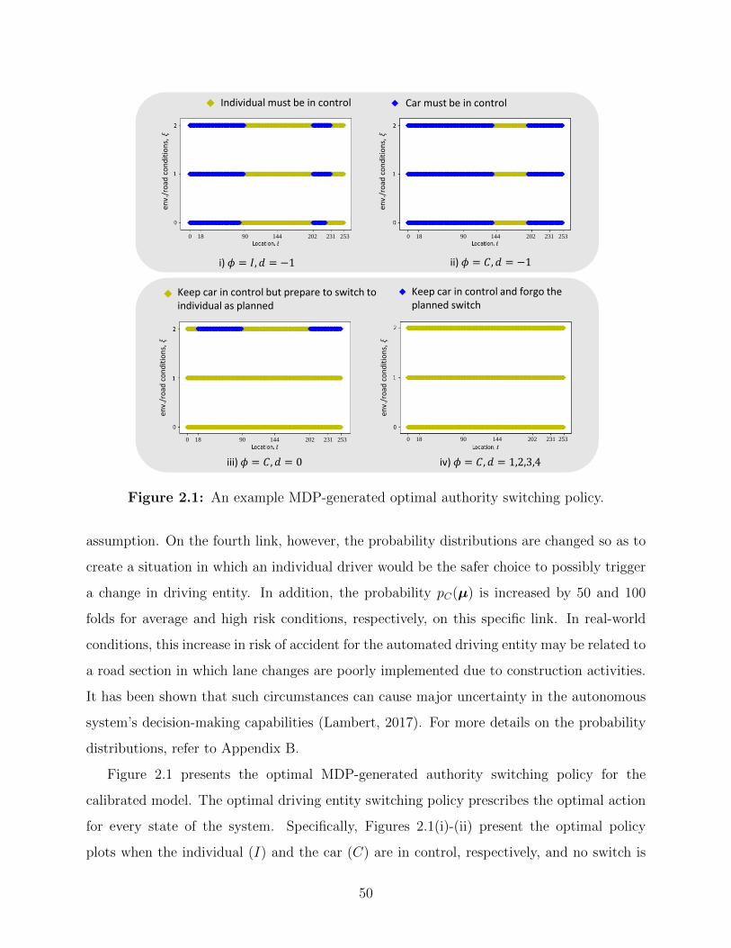
Individual must be in control Car must be in control
i) 𝜙 = 𝐼, 𝑑 = −1 ii) 𝜙 = 𝐶, 𝑑 = −1
iii) 𝜙 = 𝐶, 𝑑 = 0 iv) 𝜙 = 𝐶, 𝑑 = 1,2,3,4
Keep car in control but prepare to switch to individual as planned
Keep car in control and forgo the planned switch
env.
/ro
ad c
on
dit
ion
s, 𝜉
env.
/ro
ad c
on
dit
ion
s, 𝜉
env.
/ro
ad c
on
dit
ion
s, 𝜉
env.
/ro
ad c
on
dit
ion
s, 𝜉
0 18 90 144 202 231 253 0 18 90 144 202 231 253
0 18 90 144 202 231 253 0 18 90 144 202 231 253
Figure 2.1: An example MDP-generated optimal authority switching policy.
assumption. On the fourth link, however, the probability distributions are changed so as to
create a situation in which an individual driver would be the safer choice to possibly trigger
a change in driving entity. In addition, the probability pC(µ) is increased by 50 and 100
folds for average and high risk conditions, respectively, on this specific link. In real-world
conditions, this increase in risk of accident for the automated driving entity may be related to
a road section in which lane changes are poorly implemented due to construction activities.
It has been shown that such circumstances can cause major uncertainty in the autonomous
system’s decision-making capabilities (Lambert, 2017). For more details on the probability
distributions, refer to Appendix B.
Figure 2.1 presents the optimal MDP-generated authority switching policy for the
calibrated model. The optimal driving entity switching policy prescribes the optimal action
for every state of the system. Specifically, Figures 2.1(i)-(ii) present the optimal policy
plots when the individual (I) and the car (C) are in control, respectively, and no switch is
50
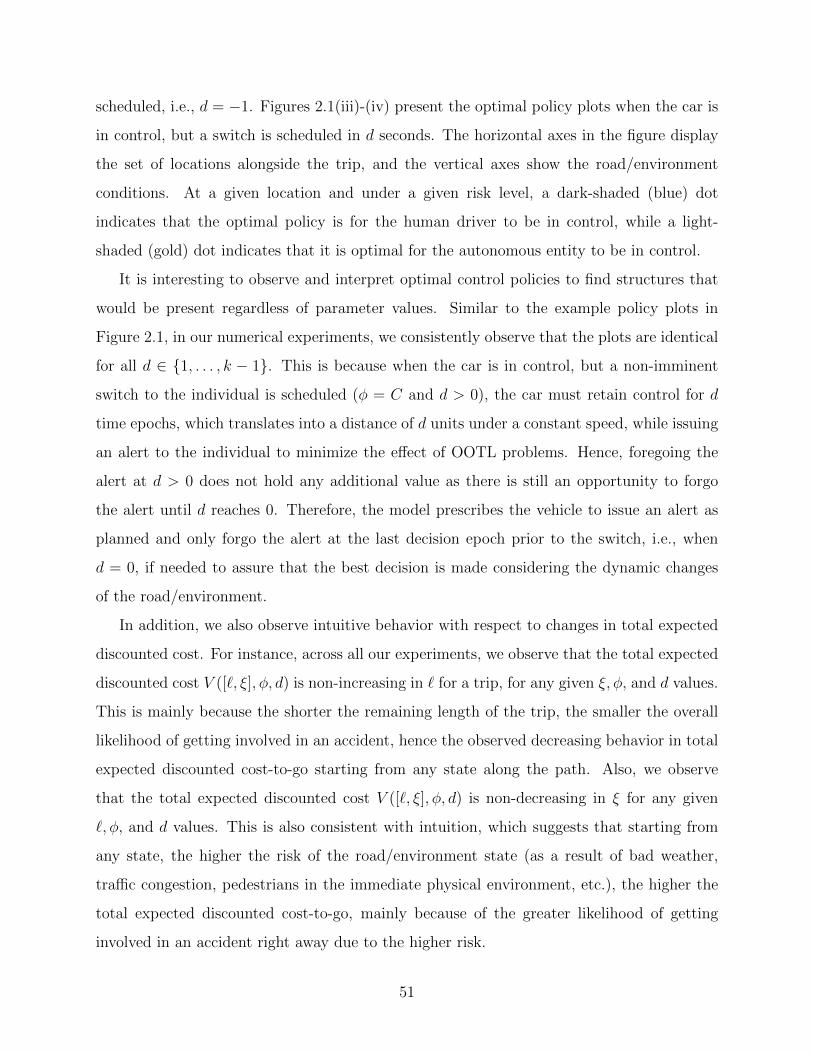
scheduled, i.e., d = −1. Figures 2.1(iii)-(iv) present the optimal policy plots when the car is
in control, but a switch is scheduled in d seconds. The horizontal axes in the figure display
the set of locations alongside the trip, and the vertical axes show the road/environment
conditions. At a given location and under a given risk level, a dark-shaded (blue) dot
indicates that the optimal policy is for the human driver to be in control, while a light-
shaded (gold) dot indicates that it is optimal for the autonomous entity to be in control.
It is interesting to observe and interpret optimal control policies to find structures that
would be present regardless of parameter values. Similar to the example policy plots in
Figure 2.1, in our numerical experiments, we consistently observe that the plots are identical
for all d ∈ {1, . . . , k − 1}. This is because when the car is in control, but a non-imminent
switch to the individual is scheduled (φ = C and d > 0), the car must retain control for d
time epochs, which translates into a distance of d units under a constant speed, while issuing
an alert to the individual to minimize the effect of OOTL problems. Hence, foregoing the
alert at d > 0 does not hold any additional value as there is still an opportunity to forgo
the alert until d reaches 0. Therefore, the model prescribes the vehicle to issue an alert as
planned and only forgo the alert at the last decision epoch prior to the switch, i.e., when
d = 0, if needed to assure that the best decision is made considering the dynamic changes
of the road/environment.
In addition, we also observe intuitive behavior with respect to changes in total expected
discounted cost. For instance, across all our experiments, we observe that the total expected
discounted cost V ([`, ξ], φ, d) is non-increasing in ` for a trip, for any given ξ, φ, and d values.
This is mainly because the shorter the remaining length of the trip, the smaller the overall
likelihood of getting involved in an accident, hence the observed decreasing behavior in total
expected discounted cost-to-go starting from any state along the path. Also, we observe
that the total expected discounted cost V ([`, ξ], φ, d) is non-decreasing in ξ for any given
`, φ, and d values. This is also consistent with intuition, which suggests that starting from
any state, the higher the risk of the road/environment state (as a result of bad weather,
traffic congestion, pedestrians in the immediate physical environment, etc.), the higher the
total expected discounted cost-to-go, mainly because of the greater likelihood of getting
involved in an accident right away due to the higher risk.
51
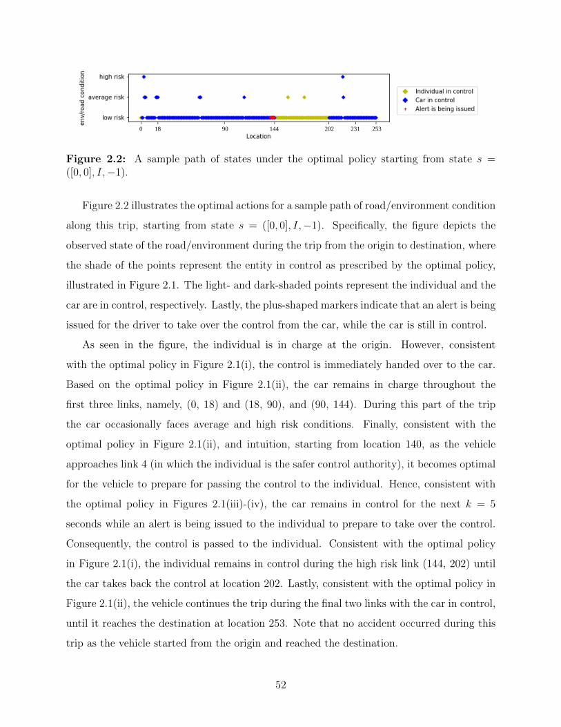
0 18 90 144 202 231 253
Figure 2.2: A sample path of states under the optimal policy starting from state s =([0, 0], I,−1).
Figure 2.2 illustrates the optimal actions for a sample path of road/environment condition
along this trip, starting from state s = ([0, 0], I,−1). Specifically, the figure depicts the
observed state of the road/environment during the trip from the origin to destination, where
the shade of the points represent the entity in control as prescribed by the optimal policy,
illustrated in Figure 2.1. The light- and dark-shaded points represent the individual and the
car are in control, respectively. Lastly, the plus-shaped markers indicate that an alert is being
issued for the driver to take over the control from the car, while the car is still in control.
As seen in the figure, the individual is in charge at the origin. However, consistent
with the optimal policy in Figure 2.1(i), the control is immediately handed over to the car.
Based on the optimal policy in Figure 2.1(ii), the car remains in charge throughout the
first three links, namely, (0, 18) and (18, 90), and (90, 144). During this part of the trip
the car occasionally faces average and high risk conditions. Finally, consistent with the
optimal policy in Figure 2.1(ii), and intuition, starting from location 140, as the vehicle
approaches link 4 (in which the individual is the safer control authority), it becomes optimal
for the vehicle to prepare for passing the control to the individual. Hence, consistent with
the optimal policy in Figures 2.1(iii)-(iv), the car remains in control for the next k = 5
seconds while an alert is being issued to the individual to prepare to take over the control.
Consequently, the control is passed to the individual. Consistent with the optimal policy
in Figure 2.1(i), the individual remains in control during the high risk link (144, 202) until
the car takes back the control at location 202. Lastly, consistent with the optimal policy in
Figure 2.1(ii), the vehicle continues the trip during the final two links with the car in control,
until it reaches the destination at location 253. Note that no accident occurred during this
trip as the vehicle started from the origin and reached the destination.
52
Table 2.1: Comparison of the optimal policy with the two benchmark policies πI and πC .
Road/environment
condition, ξ
Starting driving
entity, φ
Total expected discounted cost
Under the
optimal policy, V ∗
When only the
individual can
drive, V I
When only
the car can
drive, V C
Low riskIndividual 462.89 1,623.23 -
Car 456.29 - 937.81
Average riskIndividual 593.57 1,985.05 -
Car 579.73 - 1,061.04
High riskIndividual 1,087.46 2,582.09 -
Car 1,046.90 - 1,527.81
Table 2.1 presents the total expected discounted cost obtained starting from the
origin when no switch is scheduled, i.e., d = −1, under various initial road/environment
conditions, ξ, and entities in charge, φ. First note that, as expected, the worse the initial
road/environment condition, the higher the total expected discounted cost of the trip under
any given policy. More importantly, as seen in the table, the cost under the optimal policy
is much lower, compared with that under the two benchmark policies. Note that the cost
corresponding to πI is generally higher than under πC as the model calibration renders the
car as the generally safer option, except in the fourth link (144, 202).
Additional Metrics
In the following, we introduce a number of additional metrics to quantify risks associated
with different policies and facilitate their comparison.
Total expected discounted risk of accidents under policy πχ, Rχ(µ, φ, d). This
metric calculates the total expected discounted likelihood of accident during a trip, starting
from the state s = (µ, φ, d), under a given driving entity switching policy πχ ∈ {π∗, πC , πI}.
The risks consist of the probability of accident while driving with the entity in charge due
to location/environment-related reasons and when switching the driving entity.
To calculate the total expected discounted risk, we first slightly modify the formulations
presented in Section 2.2 to allow the model to accumulate risks, instead of costs. Then,
we conduct policy evaluation where we fix the input policy and use the new formulation to
53
recursively calculate the total expected discounted risk starting from any starting state. We
let aχ(s) denote the action in state s under policy πχ.
First note that we set the risk-to-go equal to 0 when the problem terminates. Hence,
analogous to equation (2.2) we have
Rχ([`D, ξ], φ, d) = 0 ∀ξ, φ, d. (2.10)
Recall that starting from Section 2.3, we set the vehicle to advance a unit of distance per time
period, hence the removal of dependency on time. Furthermore, we modify the immediate
cost functions to capture immediate risks. That is, we set the cost vector [c0, c1, c2] to an
all-ones vector, i.e., [1, 1, 1], in equation (2.1). This results in β(φ,µ) = 1 and γ(φ,µ) = 1,
simply capturing risk instead of cost. Hence, for instance, analogous to equation (2.3), the
total expected discounted risk under policy πχ, starting from state s = (µ, I,−1), is given
by
Rχ(µ, I,−1) = (2.11)pI(µ) + (1− pI(µ)) ·
∑ξ′∈Ξ p(ξ
′|ξ) · α ·Rχ([`+ 1, ξ′], I,−1) if aχ(s) = I,
ζC(µ) + (1− ζC(µ))[pC(µ) + (1− pC(µ)) ·
∑ξ′∈Ξ p(ξ
′|ξ) · α
·Rχ([`+ 1, ξ′], C,−1)]
if aχ(s) = C.
In addition, we set the cost of alerting the individual to take over the control, cA, and the
penalty cost of foregoing a planned switch in authority, cP , to 0, i.e., cA = cP = 0. Hence,
equations (2.4)-(2.6) may also be re-written to only account for risks.
Total expected discounted risk of accidents due to location/environment-related
reasons under policy πχ, Rχe (µ, φ, d). This metric calculates the total expected discounted
likelihood of accident during a trip due to location/environment-related reasons, starting
from state s = (µ, φ, d), under a given driving entity switching policy πχ ∈ {π∗, πC , πI}.
Similar to the previous metric, we calculate this metric by modifying the formulations
presented in Section 2.2. Specifically, to calculate Rχe (s), we use the formulations used
to calculate Rχ(s) where we also set γ(φ,µ) equal to zero to only account for the
location/environment-related risks.
54
Total expected discounted risk of accidents due to switching driving entities
under policy πχ, Rχs (µ, φ, d). Lastly, this metric calculates the total expected discounted
likelihood of accidents during a trip due to switching the driving entity, starting from the state
s = (µ, φ, d), under a given driving entity switching policy πχ ∈ {π∗, πC , πI}. Similar to the
previous metric, we calculate this metric by modifying the formulations presented in Section
2.2. Specifically, to calculate Rχs (s), we use the formulations used to calculate Rχ(s) where
we also set β(φ,µ) equal to zero to only account for the driving entity switching-related risks.
Note that in this study we overall define two categories of risks, i.e., Rχ(s) = Rχs (s) +
Rχe (s). In addition, note that starting any state s, under policies πχ ∈ {πC , πI}, Rχ(s) =
Rχe (s) and Rχ
s (s) = 0 because these policies are single entity driving policies, without any
possibilities for switching.
Sensitivity and Robustness Analyses
In this section, we investigate the effect of various model parameters on the results under the
optimal and benchmark policies. Specifically, we first investigate the impact of trip length
on the results. We then fix the trip length and examine the impact of parameters such as
road-environment dynamics and probability of accident by the driving entities. To facilitate
these comparisons, we use various performance metrics, including cost and risks, during
entire trips by using starting states so = ([0, 0], φ,−1), i.e., starting at location `O = 0 under
a low risk road/environment state ξ = 0, with driving entity φ, when no switch in authority
is scheduled, d = −1. Note that under the benchmark policies πI and πC , we use the starting
states in which the value of φ equals to I and C, respectively. Under the optimal policy
π∗, we report the best performance metric obtained starting with either φ = I or φ = C.
Because the models are calibrated with simulated data, we repeat all analyses 25 times to
assure that the results are not biased and to also provide a 95% confidence interval (CI) for
the reported means.
First, we investigate the impact of trip length on the results, when all else is held constant.
To do so, we simulate a trip, consisting of a given number of equal length links, where
accident-related probabilities are randomly generated (see Appendix B). We then scale the
links to generate three sets of trips with lengths 500, 1000, and 1500 units. As a result, any
55
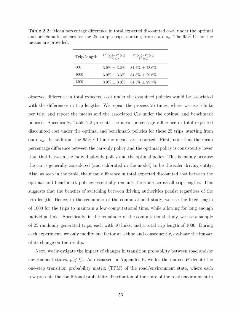
Table 2.2: Mean percentage difference in total expected discounted cost, under the optimaland benchmark policies for the 25 sample trips, starting from state so. The 95% CI for themeans are provided.
Trip length V C(so)−V ∗(so)V ∗(so)
V I(so)−V ∗(so)V ∗(so)
500 3.9% ± 3.2% 84.4% ± 28.6%
1000 3.9% ± 3.3% 84.3% ± 29.6%
1500 3.9% ± 3.3% 84.3% ± 29.7%
observed difference in total expected cost under the examined policies would be associated
with the differences in trip lengths. We repeat the process 25 times, where we use 5 links
per trip, and report the means and the associated CIs under the optimal and benchmark
policies. Specifically, Table 2.2 presents the mean percentage difference in total expected
discounted cost under the optimal and benchmark policies for these 25 trips, starting from
state so. In addition, the 95% CI for the means are reported. First, note that the mean
percentage difference between the car-only policy and the optimal policy is consistently lower
than that between the individual-only policy and the optimal policy. This is mainly because
the car is generally considered (and calibrated in the model) to be the safer driving entity.
Also, as seen in the table, the mean difference in total expected discounted cost between the
optimal and benchmark policies essentially remains the same across all trip lengths. This
suggests that the benefits of switching between driving authorities persist regardless of the
trip length. Hence, in the remainder of the computational study, we use the fixed length
of 1000 for the trips to maintain a low computational time, while allowing for long enough
individual links. Specifically, in the remainder of the computational study, we use a sample
of 25 randomly generated trips, each with 10 links, and a total trip length of 1000. During
each experiment, we only modify one factor at a time and consequently, evaluate the impact
of its change on the results.
Next, we investigate the impact of changes in transition probability between road and/or
environment states, p(ξ′|ξ). As discussed in Appendix B, we let the matrix P denote the
one-step transition probability matrix (TPM) of the road/environment state, where each
row presents the conditional probability distribution of the state of the road/environment in
56
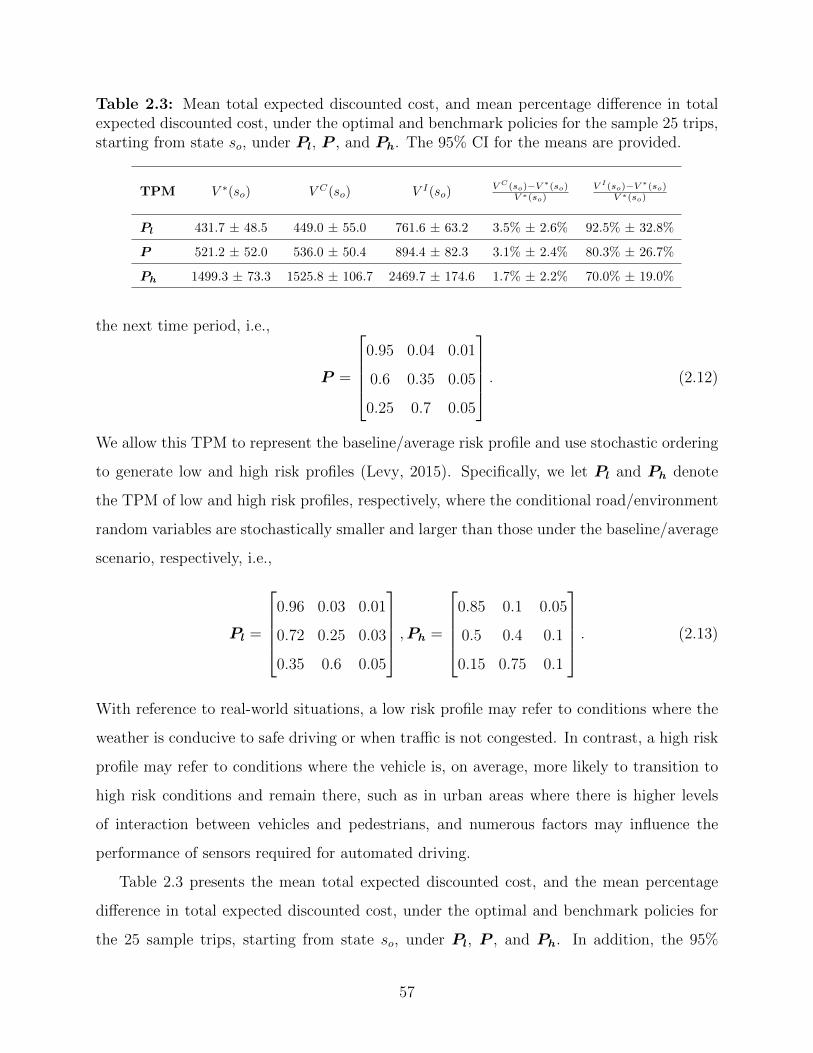
Table 2.3: Mean total expected discounted cost, and mean percentage difference in totalexpected discounted cost, under the optimal and benchmark policies for the sample 25 trips,starting from state so, under Pl, P , and Ph. The 95% CI for the means are provided.
TPM V ∗(so) V C(so) V I(so)V C(so)−V ∗(so)
V ∗(so)V I(so)−V ∗(so)
V ∗(so)
Pl 431.7 ± 48.5 449.0 ± 55.0 761.6 ± 63.2 3.5% ± 2.6% 92.5% ± 32.8%
P 521.2 ± 52.0 536.0 ± 50.4 894.4 ± 82.3 3.1% ± 2.4% 80.3% ± 26.7%
Ph 1499.3 ± 73.3 1525.8 ± 106.7 2469.7 ± 174.6 1.7% ± 2.2% 70.0% ± 19.0%
the next time period, i.e.,
P =
0.95 0.04 0.01
0.6 0.35 0.05
0.25 0.7 0.05
. (2.12)
We allow this TPM to represent the baseline/average risk profile and use stochastic ordering
to generate low and high risk profiles (Levy, 2015). Specifically, we let Pl and Ph denote
the TPM of low and high risk profiles, respectively, where the conditional road/environment
random variables are stochastically smaller and larger than those under the baseline/average
scenario, respectively, i.e.,
Pl =
0.96 0.03 0.01
0.72 0.25 0.03
0.35 0.6 0.05
,Ph =
0.85 0.1 0.05
0.5 0.4 0.1
0.15 0.75 0.1
. (2.13)
With reference to real-world situations, a low risk profile may refer to conditions where the
weather is conducive to safe driving or when traffic is not congested. In contrast, a high risk
profile may refer to conditions where the vehicle is, on average, more likely to transition to
high risk conditions and remain there, such as in urban areas where there is higher levels
of interaction between vehicles and pedestrians, and numerous factors may influence the
performance of sensors required for automated driving.
Table 2.3 presents the mean total expected discounted cost, and the mean percentage
difference in total expected discounted cost, under the optimal and benchmark policies for
the 25 sample trips, starting from state so, under Pl, P , and Ph. In addition, the 95%
57
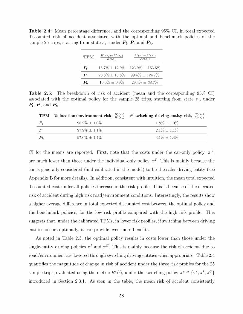
Table 2.4: Mean percentage difference, and the corresponding 95% CI, in total expecteddiscounted risk of accident associated with the optimal and benchmark policies of thesample 25 trips, starting from state so, under Pl, P , and Ph.
TPM RC(so)−R∗(so)R∗(so)
RI(so)−R∗(so)R∗(so)
Pl 16.7% ± 12.9% 123.9% ± 163.6%
P 20.8% ± 15.8% 99.4% ± 124.7%
Ph 10.0% ± 9.9% 29.4% ± 38.7%
Table 2.5: The breakdown of risk of accident (mean and the corresponding 95% CI)associated with the optimal policy for the sample 25 trips, starting from state so, underPl, P , and Ph.
TPM % location/environment risk,R∗
e(so)R∗(so) % switching driving entity risk,
R∗s(so)
R∗(so)
Pl 98.2% ± 1.0% 1.8% ± 1.0%
P 97.9% ± 1.1% 2.1% ± 1.1%
Ph 97.0% ± 1.4% 3.1% ± 1.4%
CI for the means are reported. First, note that the costs under the car-only policy, πC ,
are much lower than those under the individual-only policy, πI . This is mainly because the
car is generally considered (and calibrated in the model) to be the safer driving entity (see
Appendix B for more details). In addition, consistent with intuition, the mean total expected
discounted cost under all policies increase in the risk profile. This is because of the elevated
risk of accident during high risk road/environment conditions. Interestingly, the results show
a higher average difference in total expected discounted cost between the optimal policy and
the benchmark policies, for the low risk profile compared with the high risk profile. This
suggests that, under the calibrated TPMs, in lower risk profiles, if switching between driving
entities occurs optimally, it can provide even more benefits.
As noted in Table 2.3, the optimal policy results in costs lower than those under the
single-entity driving policies πI and πC . This is mainly because the risk of accident due to
road/environment are lowered through switching driving entities when appropriate. Table 2.4
quantifies the magnitude of change in risk of accident under the three risk profiles for the 25
sample trips, evaluated using the metric Rχ(·), under the switching policy πχ ∈ {π∗, πI , πC}
introduced in Section 2.3.1. As seen in the table, the mean risk of accident consistently
58
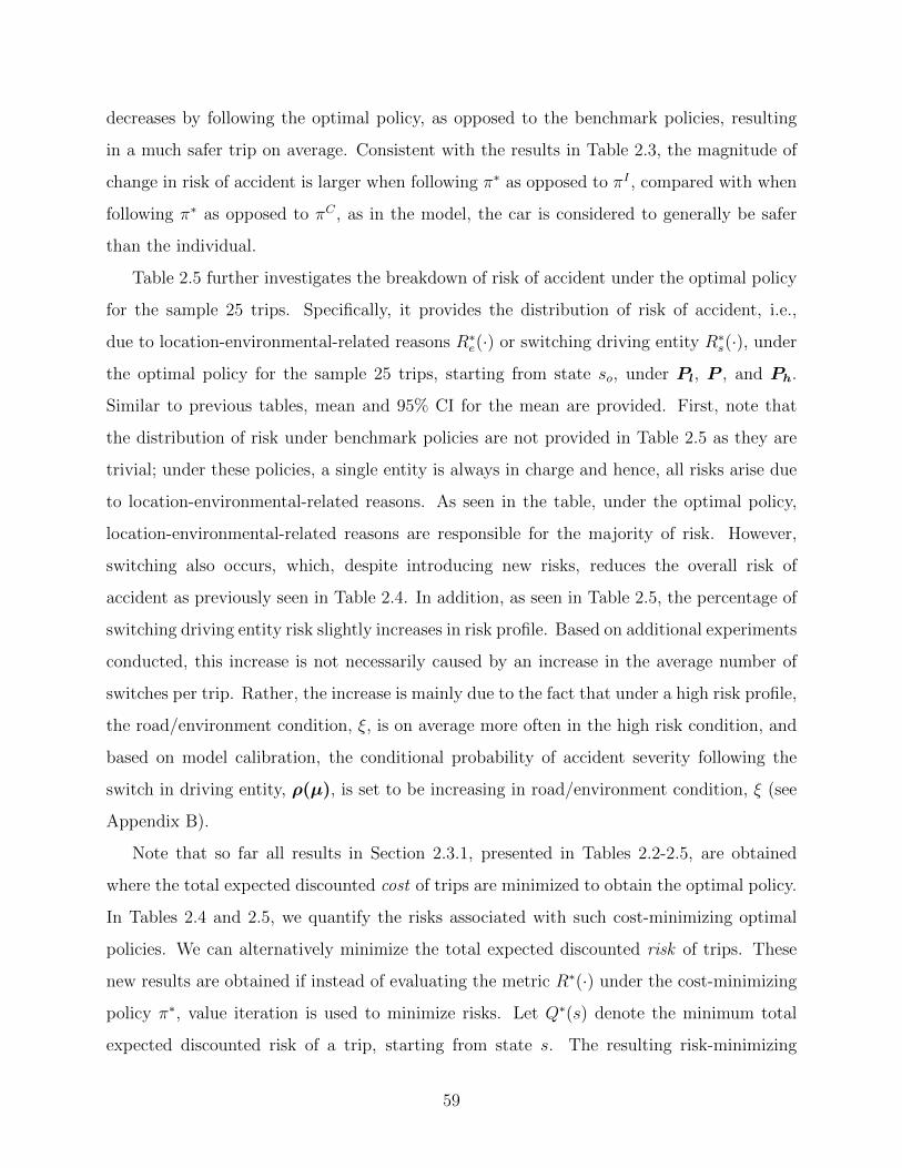
decreases by following the optimal policy, as opposed to the benchmark policies, resulting
in a much safer trip on average. Consistent with the results in Table 2.3, the magnitude of
change in risk of accident is larger when following π∗ as opposed to πI , compared with when
following π∗ as opposed to πC , as in the model, the car is considered to generally be safer
than the individual.
Table 2.5 further investigates the breakdown of risk of accident under the optimal policy
for the sample 25 trips. Specifically, it provides the distribution of risk of accident, i.e.,
due to location-environmental-related reasons R∗e(·) or switching driving entity R∗s(·), under
the optimal policy for the sample 25 trips, starting from state so, under Pl, P , and Ph.
Similar to previous tables, mean and 95% CI for the mean are provided. First, note that
the distribution of risk under benchmark policies are not provided in Table 2.5 as they are
trivial; under these policies, a single entity is always in charge and hence, all risks arise due
to location-environmental-related reasons. As seen in the table, under the optimal policy,
location-environmental-related reasons are responsible for the majority of risk. However,
switching also occurs, which, despite introducing new risks, reduces the overall risk of
accident as previously seen in Table 2.4. In addition, as seen in Table 2.5, the percentage of
switching driving entity risk slightly increases in risk profile. Based on additional experiments
conducted, this increase is not necessarily caused by an increase in the average number of
switches per trip. Rather, the increase is mainly due to the fact that under a high risk profile,
the road/environment condition, ξ, is on average more often in the high risk condition, and
based on model calibration, the conditional probability of accident severity following the
switch in driving entity, ρ(µ), is set to be increasing in road/environment condition, ξ (see
Appendix B).
Note that so far all results in Section 2.3.1, presented in Tables 2.2-2.5, are obtained
where the total expected discounted cost of trips are minimized to obtain the optimal policy.
In Tables 2.4 and 2.5, we quantify the risks associated with such cost-minimizing optimal
policies. We can alternatively minimize the total expected discounted risk of trips. These
new results are obtained if instead of evaluating the metric R∗(·) under the cost-minimizing
policy π∗, value iteration is used to minimize risks. Let Q∗(s) denote the minimum total
expected discounted risk of a trip, starting from state s. The resulting risk-minimizing
59
Table 2.6: Mean percentage difference, and the corresponding 95% CI, between theminimum total expected discounted risk of accident and the total expected discounted riskof accident under benchmark policies for the sample 25 trips, starting from state so, underPl, P , and Ph.
TPM QC(so)−Q∗(so)Q∗(so)
QI(so)−Q∗(so)Q∗(so)
Pl 47.7% ± 22.0% 146.6% ± 166.9%
P 45.4% ± 21.0% 115.5% ± 122.3%
Ph 32.9% ± 14.8% 43.7% ± 35.2%
driving entity switching policy treats all types of accidents the same, and essentially ignores
costs associated with different types of accidents. Table 2.6 presents the mean percentage
difference, and the corresponding 95% CI, between the minimum total expected discounted
risk of accident and the total expected discounted risk of accident under benchmark policies
for the sample 25 trips, starting from state so, under Pl, P , and Ph. Compare this table
with Table 2.4. As expected, the risk-minimizing driving entity switching policy in Table
2.6 results in a larger magnitude of change in total risk, compared with the cost-minimizing
driving entity switching policy presented in Table 2.4.
Next, we conduct sensitivity analysis on the probability of accident for driving entity
φ at location-environment µ, pφ(µ). Specifically, we decrease and increase the calibrated
values for pφ(µ) along the sample 25 trips by 20% and 50%, respectively, and examine its
impact on the total expected discounted cost. Note that because pφ(µ) values are generally
low, they do not exceed 1 after the increase. Table 2.7 illustrates the mean total expected
discounted cost, and mean percentage difference in total expected discounted cost, under the
optimal and benchmark policies for the sample 25 trip starting from state so, under three
sets of probabilities of accident for the two driving entities. The 95% CI for the means are
provided. Note that as in previous cases, the costs under the car-only policy, πC , are much
lower than those under the individual-only policy, πI , because the car is calibrated in the
model to be the safer driving entity. Consistent with intuition, in Table 2.7 the mean total
expected discounted cost increases in the probability of accident under all policies. However,
it is interesting to note that the change in probability of accident does not greatly impact the
degree to which the optimal policy outperforms the single entity driving benchmark policies.
60

Table 2.7: Mean total expected discounted cost, and mean percentage difference in totalexpected discounted cost, under the optimal and benchmark policies for the sample 25 tripsstarting from state so, under the corresponding sets of probabilities of accident for the twodriving entities. The 95% CI for the means are provided.
Probability
of accidentV ∗(so) V C(so) V I(so)
V C(so)−V ∗(so)V ∗(so)
V I(so)−V ∗(so)V ∗(so)
0.5× pφ(µ) 262.7 ± 26.3 268.4 ± 25.8 449.5 ± 44.1 2.5% ± 2.3% 79.9% ± 26.9%
0.8× pφ(µ) 418.1 ± 41.8 428.9 ± 40.6 717.0 ± 70.1 3.0% ± 2.4% 80.2% ± 26.8%
pφ(µ) 521.2 ± 52.0 536.0 ± 50.4 894.4 ± 82.3 3.1% ± 2.4% 80.3% ± 26.7%
1.2× pφ(µ) 623.8 ± 64.2 640.6 ± 62.0 1071.1 ± 108.5 3.1% ± 2.4% 80.3% ± 26.6%
1.5× pφ(µ) 777.1 ± 76.9 798.2 ± 74.2 1334.8 ± 129.6 3.1% ± 2.4% 80.3% ± 26.5%
Table 2.8: Mean difference in total expected discounted cost between V χ(s), πχ ∈{π∗, πI , πC}, and U(s) for the sample 25 trips starting from state s0, for the two extremeTPMs Pl and Ph. The 95% CI for the means are provided.
Actual TPM Miss-specified TPM U(so)−V ∗(so)V ∗(so)
V C(so)−U(so)U(so)
V I(so)−U(so)U(so)
Ph Pl 0.4% ± 0.7% 1.3% ± 1.5% 69.6% ± 19.2%
Pl Ph 0.2% ± 0.4% 3.7% ± 2.5% 90.9% ± 33.3%
61

Finally, we conduct a robustness analysis to evaluate the extent to which possible
estimation errors in transition probabilities can affect the results. Specifically, we investigate
the effect of making sub-optimal switches in the driving entity as a result of using a miss-
specified TPM. Suppose a car is set to travel during rush hour, where based on historical
data, a TPM such as Ph, characterizing a high risk level, should be used to find the optimal
entity switching policy. However, suppose that on this particular day, a nearby school is
closed, which results in a less congested traffic, where based on historical data a TPM such
as Pl, characterizing a low risk profile, must indeed be used to optimize the trip. Accordingly,
in this analysis, we quantify the degree to which such miss-specification of TPM can impact
the results.
To facilitate the comparisons, we introduce a new piece of notation. Let U(s) denote the
total expected discounted cost-to-go starting from state s that is obtained when implementing
the switching policy that is optimal under a miss-specified TPM. Clearly, this policy can be
sub-optimal under the actual TPM, hence V ∗(s) ≤ U(s).
Table 2.8 illustrates the mean difference in total expected discounted cost between V χ(s),
πχ ∈ {π∗, πI , πC}, and U(s) for the sample 25 trips starting from state s0, for the two
extreme TPMs Pl and Ph. The 95% CI for the means are provided. First, note that despite
the difference between the actual and miss-specified TPMs, the mean difference between
total expected discounted cost under the optimal and miss-specified policies is relatively
small, i.e., up to 0.4% on average. Furthermore, as seen in the last two columns, using
the switching policy that is optimal under a miss-specified TPM still, on average, results in
better outcomes, compared with the single driving entity benchmark policies. Indeed, for
all of the sample 25 trips, the costs obtained under the benchmark policies starting from
the starting state, i.e., V I(s0) or V C(s0), are never lower than those obtained under the
miss-specified TPM, U(s0).
2.3.2 Computational Study Under Partial Information
In this section, we perform numerical experiments to investigate the case where the
environmental risk factor is partially observable to the system. As a result, we use the
POMDP model solved using the A3C algorithm. We first illustrate the capability of A3C
62
to solve a fully observable case, i.e., the MDP case, for a specific trip setting. Specifically,
we compare the cost under the A3C policy compared to the benchmark policies where only
the car or individual can drive throughout a trip. We then investigate cases where the
environmental risk is observable to different degrees.
We let πA denote the (near-)optimal policy obtained from solving the POMDP model
using A3C. Recall that π∗ denotes the optimal policy, and πC and πI denote the policies
where only the car or the individual can drive, respectively. Analogous to the fully observable
case, to facilitate comparisons, we evaluate the total expected discounted costs starting from
zo = (0, [1, 0, 0], φ,−1), i.e., starting at location `O = 0, under the belief that we are in a low
risk road/environment state b = [1, 0, 0], with driving entity φ, when no switch in authority is
scheduled, d = −1. Lastly, we let W χ(z) denote the total expected discounted cost obtained
starting from state z under policy πχ ∈ {πA, πC , πI}. To obtain W χ(z), we conduct forward
simulation using the formulation in Section 2.2.2 to obtain the total expected discounted
cost starting from state z. Specifically, we simulate 50,000 random sample paths according
to the particular trip setting of interest, which we let the vehicle navigate while following
the policy πχ. We then report the average total expected discounted cost over the 50,000
sample paths as W χ(z).
To illustrate the capability of A3C solving a fully observable case, we generate an example
trip. The path and its junction points are as follows: [0, 26, 39, 50], with the following link
lengths from the origin to the destination: [26, 13, 11]. This path may be interpreted as
follows: Starting from the origin, i.e., location 0, the vehicle first needs to traverse a link of
length 26 units to reach location 26. From this location, the vehicle needs to travel through
a link of length 13 units to reach location 39. Finally, the vehicle reaches the destination at
location 50 after traversing the last link of length 11. In general, in this illustrative example,
the car is considered to be a safer driving entity than the individual, and the probabilities
pφ(µ) and ζφ(µ) are generated to reflect this assumption. On the second link, however, the
probability distributions are changed to create a situation in which the individual would
be the safer choice to possibly trigger a change in driving entity. As such, the probability
pC(µ) is increased by 500 folds for low, average and high risk conditions, respectively, on
this specific link. As discussed in Section 2.3.1, such increase in risk of accident for the
63
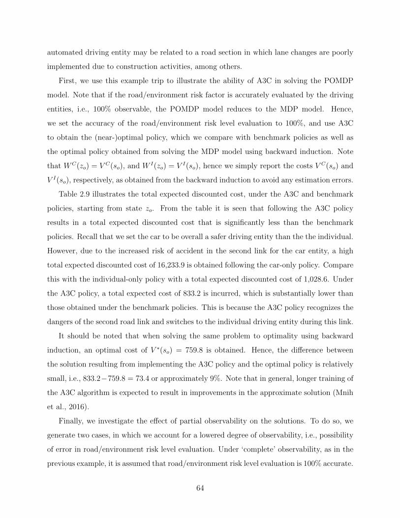
automated driving entity may be related to a road section in which lane changes are poorly
implemented due to construction activities, among others.
First, we use this example trip to illustrate the ability of A3C in solving the POMDP
model. Note that if the road/environment risk factor is accurately evaluated by the driving
entities, i.e., 100% observable, the POMDP model reduces to the MDP model. Hence,
we set the accuracy of the road/environment risk level evaluation to 100%, and use A3C
to obtain the (near-)optimal policy, which we compare with benchmark policies as well as
the optimal policy obtained from solving the MDP model using backward induction. Note
that WC(zo) = V C(so), and W I(zo) = V I(so), hence we simply report the costs V C(so) and
V I(so), respectively, as obtained from the backward induction to avoid any estimation errors.
Table 2.9 illustrates the total expected discounted cost, under the A3C and benchmark
policies, starting from state zo. From the table it is seen that following the A3C policy
results in a total expected discounted cost that is significantly less than the benchmark
policies. Recall that we set the car to be overall a safer driving entity than the the individual.
However, due to the increased risk of accident in the second link for the car entity, a high
total expected discounted cost of 16,233.9 is obtained following the car-only policy. Compare
this with the individual-only policy with a total expected discounted cost of 1,028.6. Under
the A3C policy, a total expected cost of 833.2 is incurred, which is substantially lower than
those obtained under the benchmark policies. This is because the A3C policy recognizes the
dangers of the second road link and switches to the individual driving entity during this link.
It should be noted that when solving the same problem to optimality using backward
induction, an optimal cost of V ∗(so) = 759.8 is obtained. Hence, the difference between
the solution resulting from implementing the A3C policy and the optimal policy is relatively
small, i.e., 833.2−759.8 = 73.4 or approximately 9%. Note that in general, longer training of
the A3C algorithm is expected to result in improvements in the approximate solution (Mnih
et al., 2016).
Finally, we investigate the effect of partial observability on the solutions. To do so, we
generate two cases, in which we account for a lowered degree of observability, i.e., possibility
of error in road/environment risk level evaluation. Under ‘complete’ observability, as in the
previous example, it is assumed that road/environment risk level evaluation is 100% accurate.
64
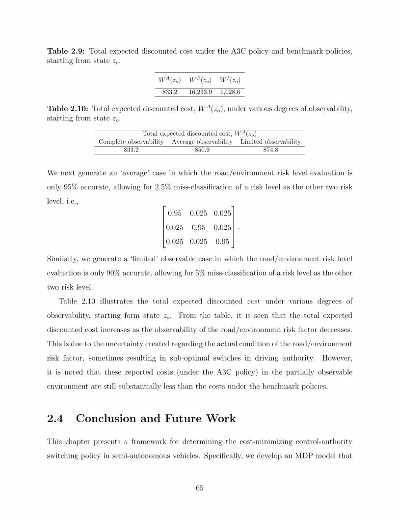
Table 2.9: Total expected discounted cost under the A3C policy and benchmark policies,starting from state zo.
WA(zo) WC(zo) W I(zo)
833.2 16,233.9 1,028.6
Table 2.10: Total expected discounted cost, WA(zo), under various degrees of observability,starting from state zo.
Total expected discounted cost, WA(zo)Complete observability Average observability Limited observability
833.2 850.9 874.8
We next generate an ‘average’ case in which the road/environment risk level evaluation is
only 95% accurate, allowing for 2.5% miss-classification of a risk level as the other two risk
level, i.e., 0.95 0.025 0.025
0.025 0.95 0.025
0.025 0.025 0.95
.Similarly, we generate a ‘limited’ observable case in which the road/environment risk level
evaluation is only 90% accurate, allowing for 5% miss-classification of a risk level as the other
two risk level.
Table 2.10 illustrates the total expected discounted cost under various degrees of
observability, starting form state zo. From the table, it is seen that the total expected
discounted cost increases as the observability of the road/environment risk factor decreases.
This is due to the uncertainty created regarding the actual condition of the road/environment
risk factor, sometimes resulting in sub-optimal switches in driving authority. However,
it is noted that these reported costs (under the A3C policy) in the partially observable
environment are still substantially less than the costs under the benchmark policies.
2.4 Conclusion and Future Work
This chapter presents a framework for determining the cost-minimizing control-authority
switching policy in semi-autonomous vehicles. Specifically, we develop an MDP model that
65
determines the authority in charge at any point along a trip, as a function of the current
location and road-environment conditions. The model considers not only the risk of accident
due to location/environmental-related reasons, but also that due to switching driving entities.
To that end, it also accounts for the current entity in charge and the time to any previously
scheduled switch to prescribe actions. The goal is to determine the optimal driving entity
at each point in time to minimize the total expected discounted safety cost of a trip. The
framework is set up such that it accounts for a delay in authority transfer to the human
driver who may be affected by OOTL. Costs are considered for false switching alerts that do
not take effect to help prevent alarm fatigue in drivers. In addition, we develop a partially
observed Markov decision process (POMDP) model where it is assumed that the risk posed
by the immediate environment is only partially observed. We solve the POMDP using the
asynchronous advantage actor-critic (A3C) algorithm.
This framework facilitates understanding and quantifying the risks and benefits involved
in the control authority transitions in semi-autonomous vehicles where the driver is expected
to take over control of the vehicle under certain conditions. In addition, with the
necessary model calibration, the framework can be used by city planners and policy makers
to investigate the type of network (e.g., urban/suburban) in which one driving entity
would outperform the other. Such an investigation would allow for the identification of
characteristics/dynamics of regions that would be appropriate candidates for certain levels
of automation, or not suitable for autonomous driving at all. Different regions can be
modeled through the one-step transition probability matrix that quantifies the dynamics of
the environment and the probability of accident for a given driving entity. In addition, such
an investigation would allow policy makers to compare and contrast the controllable factors
that make a region suitable for autonomous driving.
Before this model can be directly used in practice, it needs to be calibrated for real-
world applications. To calibrate the models, some parameters may be readily obtained
from the literature, e.g., cost of accidents. Other parameters, however, may require
additional estimation efforts. For instance, an important part of our models is a set of
probability distributions that quantify the risks of manual driving, autonomous driving,
and authority switching under various driving scenarios. Although data to estimate these
66
probability distributions with a high degree of accuracy is not readily available, it is
possible to approximate such distributions. Specifically, we use the existing literature to
obtain probability distributions for accident severity in the manual driving mode under
various driving scenarios. For autonomous driving, one could examine the failure records
of autonomous features currently on-board of vehicles (e.g., brake assist, blind spot assist,
active lane keeping assist, adaptive cruise control) to estimate the likelihood of elevated
risk due to such failures. Finally, the existing literature on driver perception-reaction times
may be used to quantify the level of driver distraction and its associated risks after being
disengaged from the driving environment for an extended period of time.
Various extensions can be considered to improve the practicality of the proposed method.
For instance, in this work, we present the optimal driving-entity switching policy given a fixed
route. Clearly, the route choice itself may impact the expected safety of a trip. Note that
conventional passenger vehicle route guidance systems aim to direct vehicles from their origin
to destination so as to minimize travel time, maximize fuel efficiency, etc., but not directly
to maximize safety as it pertains to autonomous and semi-autonomous driving. Hence, as
a future work, we aim to extend the current model to also account for dynamic routing to
maximize safety. That is, the extended model would determine the optimal path as well
as the optimal driving entity in charge, as a function of road and environmental factors, to
minimize the safety risk of a trip, or equivalently to minimize the total expected discounted
cost/harm of possible accidents. This will further increase the complexity of the model and
the number of decisions, possibly requiring the use of approximate solution strategies to
solve the problem.
67
Chapter 3
A Dynamic Deep Reinforcement
Learning-Bayesian Framework for
Anomaly Detection
68
Disclosure: This chapter is based on a paper submitted by van Wyk et al. (2019) to IEEE
Transactions on Intelligent Transportation Systems.
van Wyk, F., Watts, J., Khojandi, A. and Masoud, N., 2019. A Dynamic Deep
Reinforcement Learning-Bayesian Framework for Anomaly Detection. IEEE Transactions
on Intelligent Transportation Systems.
My contributions to this paper include: (i) the development of the problem, (ii)
reviewing the appropriate literature, (iii) the identification of study objectives, (iv) design
and conducting of the numerical experiments, (v) majority of the writing responsibilities of
the manuscript.
Abstract
The successful operation of connected and automated vehicles depends on a large number of
information sources such as on-board sensors, roadside units, cloud data, and other vehicles.
As a result, these vehicles are susceptible to false/incorrect information, originating from
malicious or non-malicious sources, which could have fatal consequences if not processed
correctly. It is therefore critical to detect and isolate anomalous and/or faulty information
in a timely manner. To do so, anomaly detection techniques should be implemented in
real-time where if the probability of anomalous information exceeds a certain threshold, the
information is dealt with accordingly. Traditionally, in the literature, the threshold that
determines if information is anomalous or not, is fixed and determined a priori. However,
this approach not only does not account for the feedback obtained during a trip on the
performance of the algorithms, but also fails to respond to potential changes in rates of
anomalies. Hence, it is important to develop an approach that can dynamically alter this
threshold in response to exogenous factors to assure reliable and robust system operation.
In this study, we develop a mathematical framework to determine the optimal dynamic
threshold of an anomaly classification algorithm in order to maximize the safety of a trip.
Specifically, we develop and pair an anomaly classification algorithm based on convolutional
neural networks (CNN), with a partially observable Markov decision process (POMDP)
model. We solve the resulting POMDP model using the asynchronous advantage actor critic
69

(A3C) deep reinforcement learning algorithm. The prescribed policy determines the optimal
level of anomaly classification threshold in real-time that maximizes the performance. Our
numerical experiments suggest that the addition of the A3C model improves the anomaly
detection performance of the CNN, resulting in high accuracy, sensitivity, and positive
predictive value.
70
3.1 Introduction
In recent times, the transportation community has directed considerable research efforts into
the development of various aspects of an intelligent transportation system (ITS). An ITS
includes numerous concepts such as traffic management, traveler information systems, and
intelligent vehicle capabilities (Ni, 2015). These measures aim to relieve traffic congestion,
improve transportation mobility, reduce emissions, enhance user experience, and improve
safety. Connected and automated vehicles (CAVs) are expected to be an integral part of
achieving the aforementioned ITS objectives (Rios-Torres and Malikopoulos, 2016).
CAVs make use of an array of sensors and communication technologies to control vehicle
operation in a safe and efficient manner. CAVs use sensors such as cameras, ultrasonic
sensors, radar, and LiDAR to capture the driving environment in order to operate the
vehicle autonomously (with varying degrees of autonomy) (NHTSA, 2013). In addition,
connected vehicles communication (V2X) is facilitated through wireless technologies such as
dedicated short range communications (DSRC) and long-term evolution-advanced (LTE-A)
which allow CAVs to transmit relevant information to other vehicles, roadside infrastructure,
and devices. The implementation of these technologies are expected to drastically reduce the
approximately 94% of serious crashes in which human error plays a decisive role (Singh, 2015).
While there are many advantages associated with the implementation of CAV technolo-
gies, the potential dangers associated with them should not be neglected. The safe operation
of CAVs is highly dependent on the information they obtain from their sensors and wireless
communication sources. As a result, there exist a great number of sources in which false
information may be present, which poses great risk to the safe operation of CAVs. The false
information may be from a malicious source, i.e., a cyber attack, or from a non-malicious
source such as faulty sensors. It should be noted that both origins of false information
represent significant threats to the safe operation of CAVs.
There is a rapidly growing body of literature illustrating the potential dangers of CAV
technologies resulting in anomalous/false information (Petit and Shladover, 2015; Koscher
et al., 2010; Weimerskirch and Gaynier, 2015; Parkinson et al., 2017). For instance,
illustrating the injection of anomalous/false information with a malicious intent, researchers
71
showed that it is possible to interfere with LiDAR systems of CAVs by artificially creating
obstacles in the perceived environment using a laser and a pulse generator (Curtis, 2015).
Illustrating the injection of false information from a source with a non-malicious intent,
researchers found that under certain environmental conditions such as bright light, heavy
snow, and poor quality of road and traffic signs, CAVs can malfunction and perceive the
driving environment incorrectly (Moavenzadeh and Lang, 2018; Field, 2017). As a result,
anomalous/false sensor values, originating from sources with malicious or non-malicious
intent, can result in dangerous circumstances for CAVs. It is therefore critical that anomaly
detection techniques are implemented to detect anomalous/faulty information in CAVs.
There exists a large body of research in anomaly detection (e.g., see surveys by (Chandola
et al., 2009; Ahmed et al., 2016)). A significant number of these anomaly detection algorithms
apply classification algorithms, where labeled data instances are used to train a model
(classifier). In the testing phase, each test instance is assigned a probability of belonging to
a certain class by the trained model. For instance, in binary classification, this probability is
translated into two classes (normal/anomalous) using an ‘a priori’ cut-off, e.g., 0.5. Generally,
the classification threshold is determined to balance sensitivity (the proportion of anomalous
instances correctly classified) and specificity (the proportion of non-anomalous instances
correctly classified). Two types of errors may occur when classifying instances: (1) classifying
an anomalous instance as normal (non-anomalous), i.e., false negatives; (2) classifying a
normal instance as anomalous, i.e., false positives. False negatives are a clear concern in
most applications. However, false positives can also have major consequences. For instance,
in the classification of anomalous sensor values, false positives may eventually lead to the
false exclusion of non-anomalous sensor data from the data fusion process. This can have a
detrimental impact on the quality of fused data and potentially compromise the autonomous
operation of the vehicle.
In the literature, classification models used to detect anomalous information are mostly
used in isolation and in a myopic manner. That is, after being built, a classification model
remains unchanged regardless of the past success rate experienced within the system of
interest (Kruegel et al., 2003). Indeed, most models, even when they are designed to be used
in an online fashion, such as throughout a CAV trip, they are simply trained to present the
72
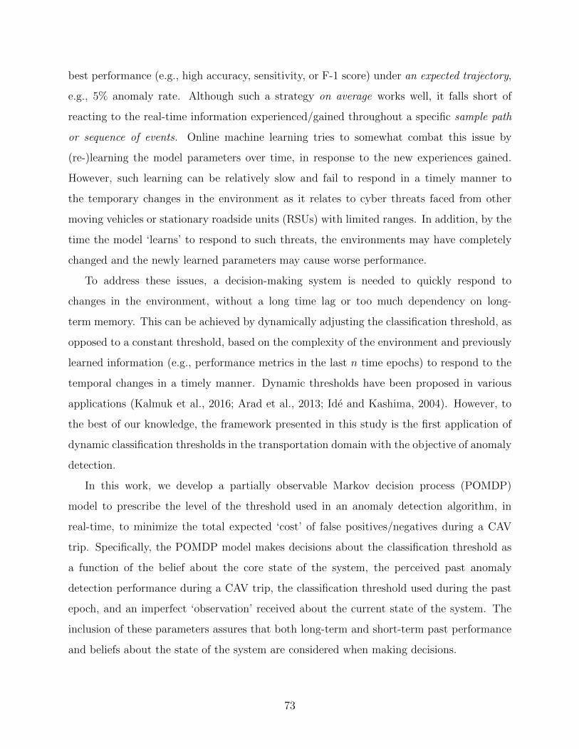
best performance (e.g., high accuracy, sensitivity, or F-1 score) under an expected trajectory,
e.g., 5% anomaly rate. Although such a strategy on average works well, it falls short of
reacting to the real-time information experienced/gained throughout a specific sample path
or sequence of events. Online machine learning tries to somewhat combat this issue by
(re-)learning the model parameters over time, in response to the new experiences gained.
However, such learning can be relatively slow and fail to respond in a timely manner to
the temporary changes in the environment as it relates to cyber threats faced from other
moving vehicles or stationary roadside units (RSUs) with limited ranges. In addition, by the
time the model ‘learns’ to respond to such threats, the environments may have completely
changed and the newly learned parameters may cause worse performance.
To address these issues, a decision-making system is needed to quickly respond to
changes in the environment, without a long time lag or too much dependency on long-
term memory. This can be achieved by dynamically adjusting the classification threshold, as
opposed to a constant threshold, based on the complexity of the environment and previously
learned information (e.g., performance metrics in the last n time epochs) to respond to the
temporal changes in a timely manner. Dynamic thresholds have been proposed in various
applications (Kalmuk et al., 2016; Arad et al., 2013; Ide and Kashima, 2004). However, to
the best of our knowledge, the framework presented in this study is the first application of
dynamic classification thresholds in the transportation domain with the objective of anomaly
detection.
In this work, we develop a partially observable Markov decision process (POMDP)
model to prescribe the level of the threshold used in an anomaly detection algorithm, in
real-time, to minimize the total expected ‘cost’ of false positives/negatives during a CAV
trip. Specifically, the POMDP model makes decisions about the classification threshold as
a function of the belief about the core state of the system, the perceived past anomaly
detection performance during a CAV trip, the classification threshold used during the past
epoch, and an imperfect ‘observation’ received about the current state of the system. The
inclusion of these parameters assures that both long-term and short-term past performance
and beliefs about the state of the system are considered when making decisions.
73
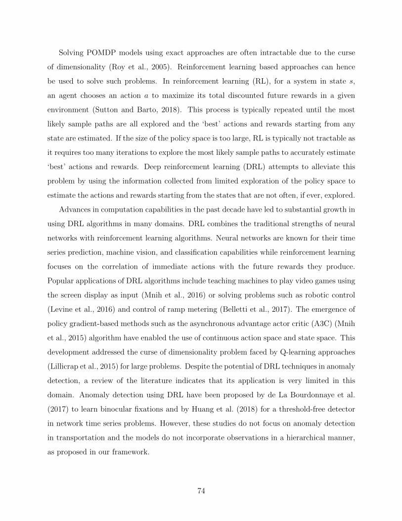
Solving POMDP models using exact approaches are often intractable due to the curse
of dimensionality (Roy et al., 2005). Reinforcement learning based approaches can hence
be used to solve such problems. In reinforcement learning (RL), for a system in state s,
an agent chooses an action a to maximize its total discounted future rewards in a given
environment (Sutton and Barto, 2018). This process is typically repeated until the most
likely sample paths are all explored and the ‘best’ actions and rewards starting from any
state are estimated. If the size of the policy space is too large, RL is typically not tractable as
it requires too many iterations to explore the most likely sample paths to accurately estimate
‘best’ actions and rewards. Deep reinforcement learning (DRL) attempts to alleviate this
problem by using the information collected from limited exploration of the policy space to
estimate the actions and rewards starting from the states that are not often, if ever, explored.
Advances in computation capabilities in the past decade have led to substantial growth in
using DRL algorithms in many domains. DRL combines the traditional strengths of neural
networks with reinforcement learning algorithms. Neural networks are known for their time
series prediction, machine vision, and classification capabilities while reinforcement learning
focuses on the correlation of immediate actions with the future rewards they produce.
Popular applications of DRL algorithms include teaching machines to play video games using
the screen display as input (Mnih et al., 2016) or solving problems such as robotic control
(Levine et al., 2016) and control of ramp metering (Belletti et al., 2017). The emergence of
policy gradient-based methods such as the asynchronous advantage actor critic (A3C) (Mnih
et al., 2015) algorithm have enabled the use of continuous action space and state space. This
development addressed the curse of dimensionality problem faced by Q-learning approaches
(Lillicrap et al., 2015) for large problems. Despite the potential of DRL techniques in anomaly
detection, a review of the literature indicates that its application is very limited in this
domain. Anomaly detection using DRL have been proposed by de La Bourdonnaye et al.
(2017) to learn binocular fixations and by Huang et al. (2018) for a threshold-free detector
in network time series problems. However, these studies do not focus on anomaly detection
in transportation and the models do not incorporate observations in a hierarchical manner,
as proposed in our framework.
74
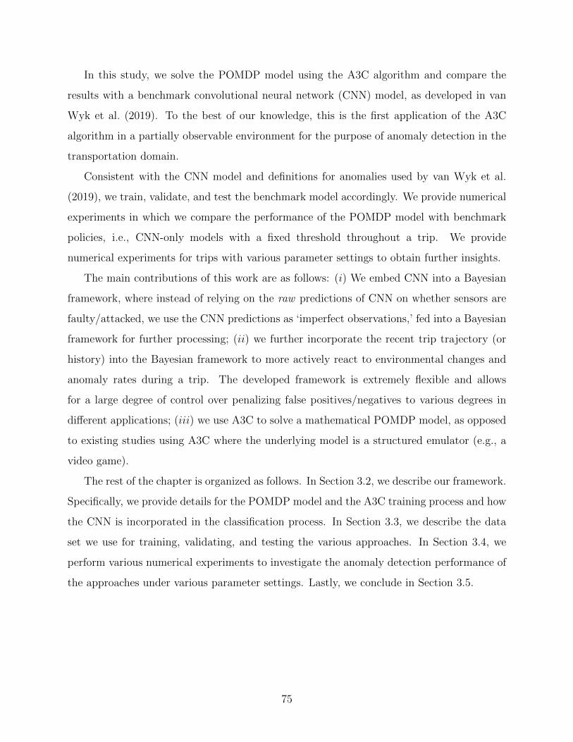
In this study, we solve the POMDP model using the A3C algorithm and compare the
results with a benchmark convolutional neural network (CNN) model, as developed in van
Wyk et al. (2019). To the best of our knowledge, this is the first application of the A3C
algorithm in a partially observable environment for the purpose of anomaly detection in the
transportation domain.
Consistent with the CNN model and definitions for anomalies used by van Wyk et al.
(2019), we train, validate, and test the benchmark model accordingly. We provide numerical
experiments in which we compare the performance of the POMDP model with benchmark
policies, i.e., CNN-only models with a fixed threshold throughout a trip. We provide
numerical experiments for trips with various parameter settings to obtain further insights.
The main contributions of this work are as follows: (i) We embed CNN into a Bayesian
framework, where instead of relying on the raw predictions of CNN on whether sensors are
faulty/attacked, we use the CNN predictions as ‘imperfect observations,’ fed into a Bayesian
framework for further processing; (ii) we further incorporate the recent trip trajectory (or
history) into the Bayesian framework to more actively react to environmental changes and
anomaly rates during a trip. The developed framework is extremely flexible and allows
for a large degree of control over penalizing false positives/negatives to various degrees in
different applications; (iii) we use A3C to solve a mathematical POMDP model, as opposed
to existing studies using A3C where the underlying model is a structured emulator (e.g., a
video game).
The rest of the chapter is organized as follows. In Section 3.2, we describe our framework.
Specifically, we provide details for the POMDP model and the A3C training process and how
the CNN is incorporated in the classification process. In Section 3.3, we describe the data
set we use for training, validating, and testing the various approaches. In Section 3.4, we
perform various numerical experiments to investigate the anomaly detection performance of
the approaches under various parameter settings. Lastly, we conclude in Section 3.5.
75
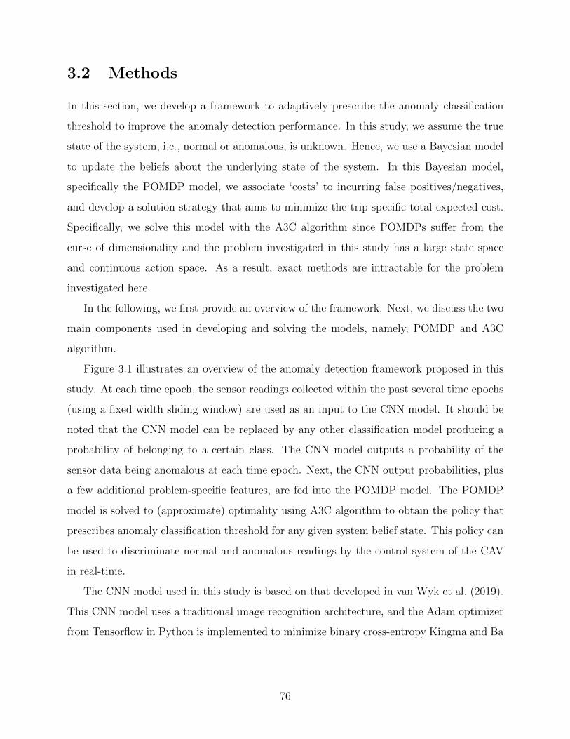
3.2 Methods
In this section, we develop a framework to adaptively prescribe the anomaly classification
threshold to improve the anomaly detection performance. In this study, we assume the true
state of the system, i.e., normal or anomalous, is unknown. Hence, we use a Bayesian model
to update the beliefs about the underlying state of the system. In this Bayesian model,
specifically the POMDP model, we associate ‘costs’ to incurring false positives/negatives,
and develop a solution strategy that aims to minimize the trip-specific total expected cost.
Specifically, we solve this model with the A3C algorithm since POMDPs suffer from the
curse of dimensionality and the problem investigated in this study has a large state space
and continuous action space. As a result, exact methods are intractable for the problem
investigated here.
In the following, we first provide an overview of the framework. Next, we discuss the two
main components used in developing and solving the models, namely, POMDP and A3C
algorithm.
Figure 3.1 illustrates an overview of the anomaly detection framework proposed in this
study. At each time epoch, the sensor readings collected within the past several time epochs
(using a fixed width sliding window) are used as an input to the CNN model. It should be
noted that the CNN model can be replaced by any other classification model producing a
probability of belonging to a certain class. The CNN model outputs a probability of the
sensor data being anomalous at each time epoch. Next, the CNN output probabilities, plus
a few additional problem-specific features, are fed into the POMDP model. The POMDP
model is solved to (approximate) optimality using A3C algorithm to obtain the policy that
prescribes anomaly classification threshold for any given system belief state. This policy can
be used to discriminate normal and anomalous readings by the control system of the CAV
in real-time.
The CNN model used in this study is based on that developed in van Wyk et al. (2019).
This CNN model uses a traditional image recognition architecture, and the Adam optimizer
from Tensorflow in Python is implemented to minimize binary cross-entropy Kingma and Ba
76
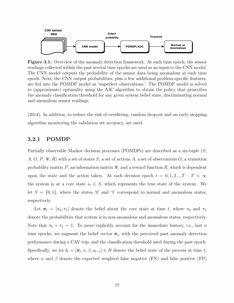
CAV sensor data
CNNmodel
Output probability
POMDP/A3C NormalorAnomalous
Threshold
Figure 3.1: Overview of the anomaly detection framework. At each time epoch, the sensorreadings collected within the past several time epochs are used as an input to the CNN model.The CNN model outputs the probability of the sensor data being anomalous at each timeepoch. Next, the CNN output probabilities, plus a few additional problem-specific features,are fed into the POMDP model as ‘imperfect observations.’ The POMDP model is solvedto (approximate) optimality using the A3C algorithm to obtain the policy that prescribesthe anomaly classification threshold for any given system belief state, discriminating normaland anomalous sensor readings.
(2014). In addition, to reduce the risk of overfitting, random dropout and an early stopping
algorithm monitoring the validation set accuracy, are used.
3.2.1 POMDP
Partially observable Markov decision processes (POMDPs) are described as a six-tuple (S,
A, O, P , Ψ, R) with a set of states S, a set of actions A, a set of observations O, a transition
probability matrix P , an information matrix Ψ, and a reward function R, which is dependent
upon the state and the action taken. At each decision epoch t = 0, 1, 2..., T : T < ∞
the system is at a core state st ∈ S, which represents the true state of the system. We
let S = {0, 1}, where the states ‘0’ and ‘1’ correspond to normal and anomalous states,
respectively.
Let πt = [π0, π1] denote the belief about the core state at time t, where π0 and π1
denote the probabilities that system is in non-anomalous and anomalous states, respectively.
Note that π0 + π1 = 1. To more explicitly account for the immediate history, i.e., last n
time epochs, we augment the belief vector πt, with the perceived past anomaly detection
performance during a CAV trip, and the classification threshold used during the past epoch.
Specifically, we let bt = [πt, α, β, at−1] ∈ B denote the belief state of the process at time t,
where α and β denote the expected weighted false negative (FN) and false positive (FP)
77

rates over the past m decision epochs, respectively, and at−1 denotes the action, i.e. the
classification threshold, used in the previous time epoch t− 1.
Recall that the system core state is only partially observable to the model. Hence,
at each time epoch t, an observation ot ∈ O = [0, 1] is made, which provides imperfect
information about the system core state. In our context, this observation is the CNN-
estimated probability that the system is in the anomalous state. Once an observation is
made, an action at ∈ A = [0, 1] is taken, as a function of belief state bt and the observation
ot to adjust the the classification threshold.
At every decision epoch, the system incurs an immediate reward as function of the action
at taken in belief state bt. This immediate reward accounts for whether the threshold chosen
is expected to correctly detect anomalous and normal readings. That is, the system is
rewarded by a unit of one for true positives (TP) and true negatives (TN), and is penalized
by a unit of one for false positives (FP) and false negatives (FN), i.e., RTP = RTN = 1
and RFP = RFN = −1. In addition, it is further rewarded/penalized based on the weighted
expected rates of FN and FP in the past m time epochs in addition to the current expected
value. The rewards function R(·) is as follows:
Rt(b, o, a) =π0 ·RTN + π1 ·RFN + α ·RFN , if ot < at,
π0 ·RFP + π1 ·RTP + β ·RFP , if ot ≥ at.
In the beginning of time epoch t + 1, the belief state bt is updated to obtain bt+1.
Specifically, the belief about the new core state s′ ∈ S at time t+ 1 is updated as follows:
πs′ =
Ψ(1{o>a}|s′
) ∑s∈S
P (s′|s) · πs∑o∈O
Ψ(1{o>a}|s′
) ∑s∈S
P (s′|s) · πs(3.1)
where P (s′|s) denotes the probability that system core state transitions from state s
to state s′, and Ψ(1{o>a}|s′
)denotes the probability that the observed system state is
anomalous/non-anomalous given the core state s′.
78
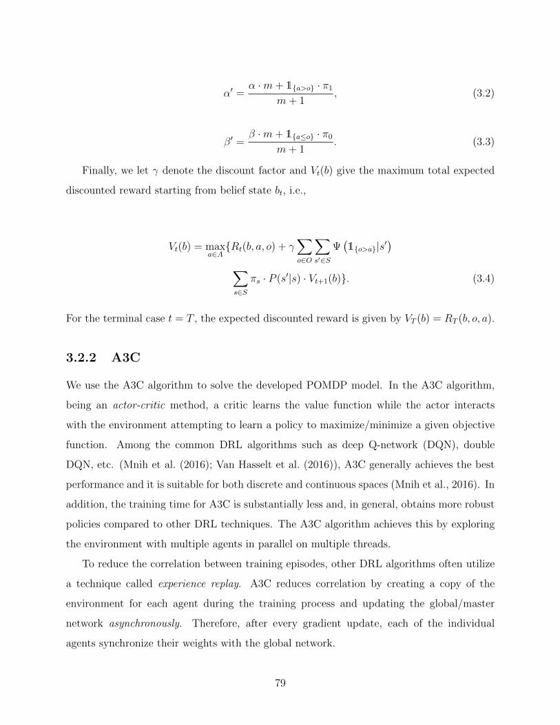
α′ =α ·m+ 1{a>o} · π1
m+ 1, (3.2)
β′ =β ·m+ 1{a≤o} · π0
m+ 1. (3.3)
Finally, we let γ denote the discount factor and Vt(b) give the maximum total expected
discounted reward starting from belief state bt, i.e.,
Vt(b) = maxa∈A{Rt(b, a, o) + γ
∑o∈O
∑s′∈S
Ψ(1{o>a}|s′
)∑s∈S
πs · P (s′|s) · Vt+1(b)}. (3.4)
For the terminal case t = T , the expected discounted reward is given by VT (b) = RT (b, o, a).
3.2.2 A3C
We use the A3C algorithm to solve the developed POMDP model. In the A3C algorithm,
being an actor-critic method, a critic learns the value function while the actor interacts
with the environment attempting to learn a policy to maximize/minimize a given objective
function. Among the common DRL algorithms such as deep Q-network (DQN), double
DQN, etc. (Mnih et al. (2016); Van Hasselt et al. (2016)), A3C generally achieves the best
performance and it is suitable for both discrete and continuous spaces (Mnih et al., 2016). In
addition, the training time for A3C is substantially less and, in general, obtains more robust
policies compared to other DRL techniques. The A3C algorithm achieves this by exploring
the environment with multiple agents in parallel on multiple threads.
To reduce the correlation between training episodes, other DRL algorithms often utilize
a technique called experience replay. A3C reduces correlation by creating a copy of the
environment for each agent during the training process and updating the global/master
network asynchronously. Therefore, after every gradient update, each of the individual
agents synchronize their weights with the global network.
79

The A3C algorithm (Mnih et al., 2016) maintains a policy π(at|st;φ), where at denotes
the action at time t, st denotes the state, and φ denotes the parameters of the global
actor network. The algorithm also estimates a value function V (st;φv), for state st using
parameters φv for the global critic network. The value function is updated with n-step
returns. The policy and the value networks are updated after every episode of length tmax
or when a terminal state is reached.
The A3C algorithm uses advantage, as opposed to Q-values in many other DRL
algorithms, to estimate how advantageous certain actions are for a particular state. The
advantage function A(·) is estimated as follows:
A(st, at;φ, φv) =k−1∑i=0
γirt+i + γkV (st+k;φv)− V (st;φv), (3.5)
where k is bounded above by tmax.
The gradient update to minimize total loss can be seen as
∇φ′ logπ(at|st;φ′)A(st, at;φ, φv), (3.6)
where φ′ is the thread-specific network parameters. Also, Mnih et al. (2016) found that if the
entropy of policy π is added to the objective function, exploration is encouraged which limits
the premature convergence to sub-optimal deterministic policies. As a result, the gradient
of the objective function which includes an entropy regularization term with respect to the
policy parameters is given as
∇φ′ logπ(at|st;φ′)A(st, at;φ, φv) + η∇φ′H(π(st;φ′)), (3.7)
where H is the policy entropy and the parameter η controls the strength of the entropy
regularization term.
To solve the POMDP model with the A3C algorithm, we use TensorFlow (Abadi et al.,
2016) in Python where we utilize the RMSProp optimizer (Tieleman and Hinton, 2012) for
training the neural networks of the actor and critic. Table 3.1 illustrates a summary of the
hyperparameters used in the model during the training process.
80
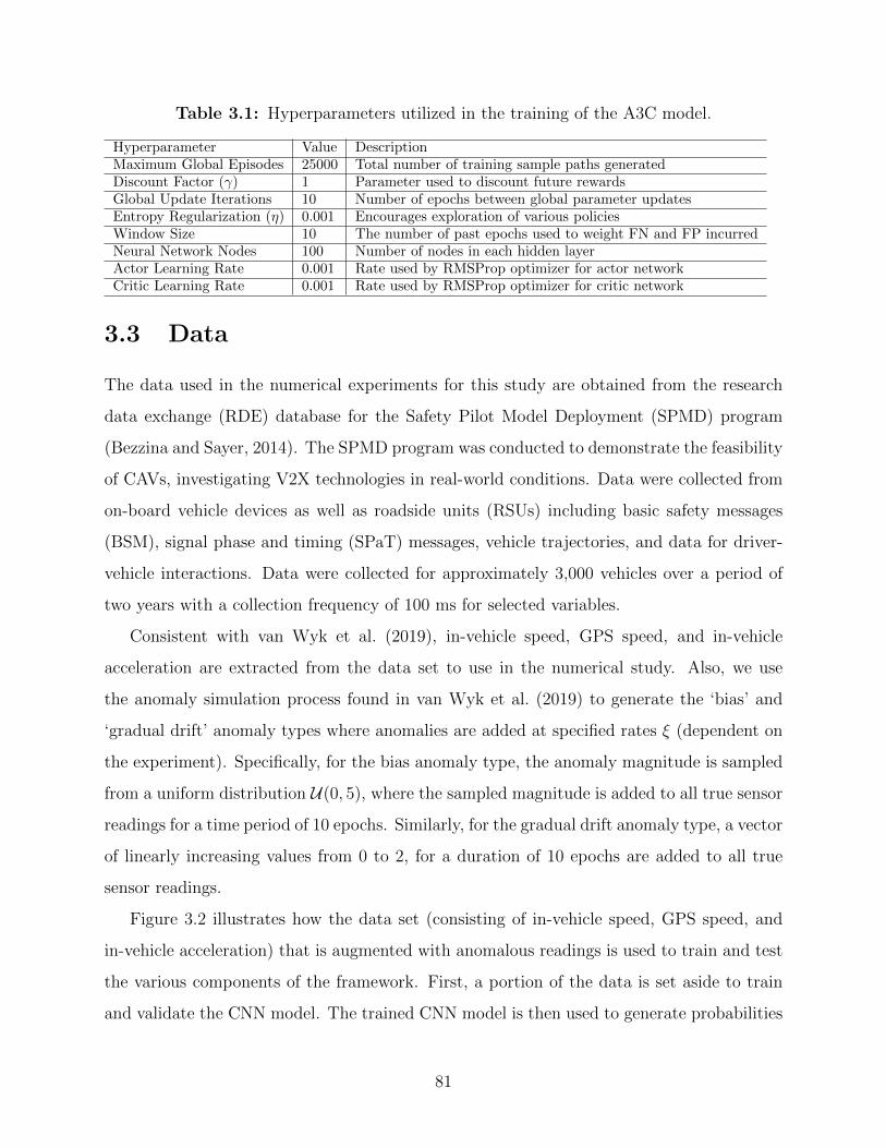
Table 3.1: Hyperparameters utilized in the training of the A3C model.
Hyperparameter Value DescriptionMaximum Global Episodes 25000 Total number of training sample paths generatedDiscount Factor (γ) 1 Parameter used to discount future rewardsGlobal Update Iterations 10 Number of epochs between global parameter updatesEntropy Regularization (η) 0.001 Encourages exploration of various policiesWindow Size 10 The number of past epochs used to weight FN and FP incurredNeural Network Nodes 100 Number of nodes in each hidden layerActor Learning Rate 0.001 Rate used by RMSProp optimizer for actor networkCritic Learning Rate 0.001 Rate used by RMSProp optimizer for critic network
3.3 Data
The data used in the numerical experiments for this study are obtained from the research
data exchange (RDE) database for the Safety Pilot Model Deployment (SPMD) program
(Bezzina and Sayer, 2014). The SPMD program was conducted to demonstrate the feasibility
of CAVs, investigating V2X technologies in real-world conditions. Data were collected from
on-board vehicle devices as well as roadside units (RSUs) including basic safety messages
(BSM), signal phase and timing (SPaT) messages, vehicle trajectories, and data for driver-
vehicle interactions. Data were collected for approximately 3,000 vehicles over a period of
two years with a collection frequency of 100 ms for selected variables.
Consistent with van Wyk et al. (2019), in-vehicle speed, GPS speed, and in-vehicle
acceleration are extracted from the data set to use in the numerical study. Also, we use
the anomaly simulation process found in van Wyk et al. (2019) to generate the ‘bias’ and
‘gradual drift’ anomaly types where anomalies are added at specified rates ξ (dependent on
the experiment). Specifically, for the bias anomaly type, the anomaly magnitude is sampled
from a uniform distribution U(0, 5), where the sampled magnitude is added to all true sensor
readings for a time period of 10 epochs. Similarly, for the gradual drift anomaly type, a vector
of linearly increasing values from 0 to 2, for a duration of 10 epochs are added to all true
sensor readings.
Figure 3.2 illustrates how the data set (consisting of in-vehicle speed, GPS speed, and
in-vehicle acceleration) that is augmented with anomalous readings is used to train and test
the various components of the framework. First, a portion of the data is set aside to train
and validate the CNN model. The trained CNN model is then used to generate probabilities
81
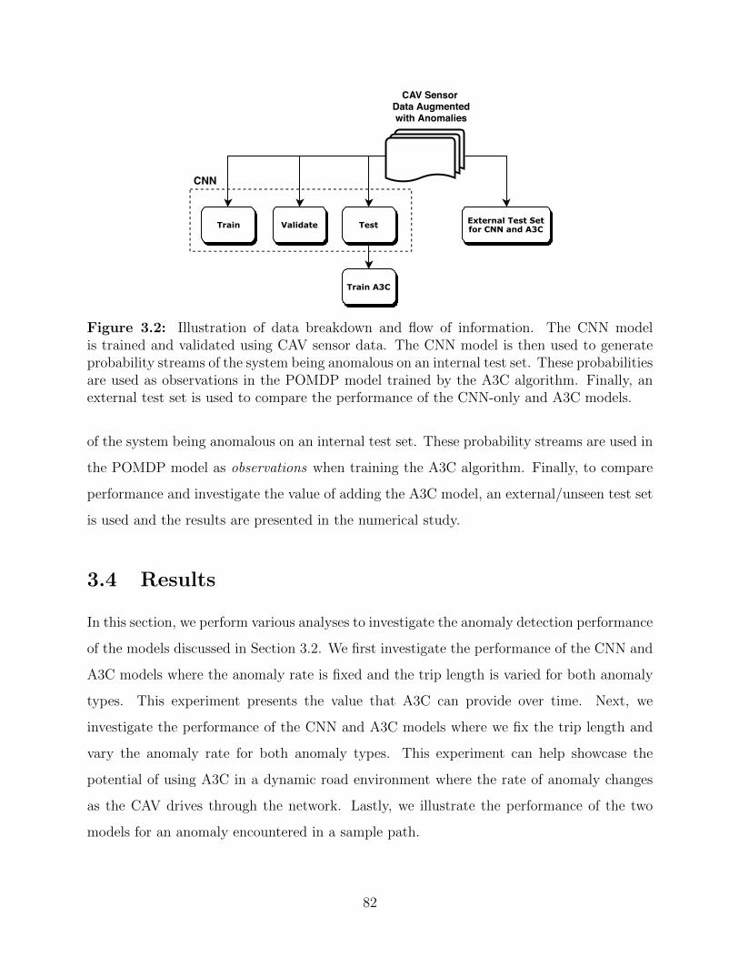
CAV Sensor Data Augmentedwith Anomalies
Train Validate ExternalTestSetforCNNandA3CTest
TrainA3C
CNN
Figure 3.2: Illustration of data breakdown and flow of information. The CNN modelis trained and validated using CAV sensor data. The CNN model is then used to generateprobability streams of the system being anomalous on an internal test set. These probabilitiesare used as observations in the POMDP model trained by the A3C algorithm. Finally, anexternal test set is used to compare the performance of the CNN-only and A3C models.
of the system being anomalous on an internal test set. These probability streams are used in
the POMDP model as observations when training the A3C algorithm. Finally, to compare
performance and investigate the value of adding the A3C model, an external/unseen test set
is used and the results are presented in the numerical study.
3.4 Results
In this section, we perform various analyses to investigate the anomaly detection performance
of the models discussed in Section 3.2. We first investigate the performance of the CNN and
A3C models where the anomaly rate is fixed and the trip length is varied for both anomaly
types. This experiment presents the value that A3C can provide over time. Next, we
investigate the performance of the CNN and A3C models where we fix the trip length and
vary the anomaly rate for both anomaly types. This experiment can help showcase the
potential of using A3C in a dynamic road environment where the rate of anomaly changes
as the CAV drives through the network. Lastly, we illustrate the performance of the two
models for an anomaly encountered in a sample path.
82
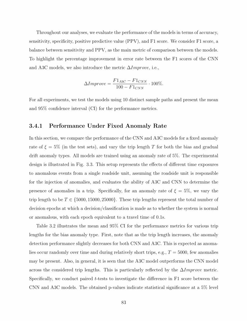
Throughout our analyses, we evaluate the performance of the models in terms of accuracy,
sensitivity, specificity, positive predictive value (PPV), and F1 score. We consider F1 score, a
balance between sensitivity and PPV, as the main metric of comparison between the models.
To highlight the percentage improvement in error rate between the F1 scores of the CNN
and A3C models, we also introduce the metric ∆Improve, i.e.,
∆Improve =F1A3C − F1CNN
100− F1CNN· 100%.
For all experiments, we test the models using 10 distinct sample paths and present the mean
and 95% confidence interval (CI) for the performance metrics.
3.4.1 Performance Under Fixed Anomaly Rate
In this section, we compare the performance of the CNN and A3C models for a fixed anomaly
rate of ξ = 5% (in the test sets), and vary the trip length T for both the bias and gradual
drift anomaly types. All models are trained using an anomaly rate of 5%. The experimental
design is illustrated in Fig. 3.3. This setup represents the effects of different time exposures
to anomalous events from a single roadside unit, assuming the roadside unit is responsible
for the injection of anomalies, and evaluates the ability of A3C and CNN to determine the
presence of anomalies in a trip. Specifically, for an anomaly rate of ξ = 5%, we vary the
trip length to be T ∈ {5000, 15000, 25000}. These trip lengths represent the total number of
decision epochs at which a decision/classification is made as to whether the system is normal
or anomalous, with each epoch equivalent to a travel time of 0.1s.
Table 3.2 illustrates the mean and 95% CI for the performance metrics for various trip
lengths for the bias anomaly type. First, note that as the trip length increases, the anomaly
detection performance slightly decreases for both CNN and A3C. This is expected as anoma-
lies occur randomly over time and during relatively short trips, e.g., T = 5000, few anomalies
may be present. Also, in general, it is seen that the A3C model outperforms the CNN model
across the considered trip lengths. This is particularly reflected by the ∆Improve metric.
Specifically, we conduct paired t-tests to investigate the difference in F1 score between the
CNN and A3C models. The obtained p-values indicate statistical significance at a 5% level
83
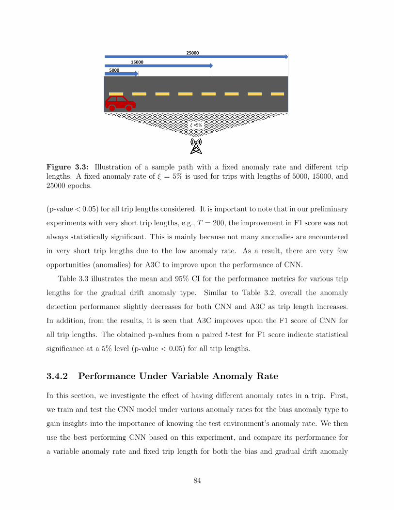
! =5%
5000
25000
15000
Figure 3.3: Illustration of a sample path with a fixed anomaly rate and different triplengths. A fixed anomaly rate of ξ = 5% is used for trips with lengths of 5000, 15000, and25000 epochs.
(p-value < 0.05) for all trip lengths considered. It is important to note that in our preliminary
experiments with very short trip lengths, e.g., T = 200, the improvement in F1 score was not
always statistically significant. This is mainly because not many anomalies are encountered
in very short trip lengths due to the low anomaly rate. As a result, there are very few
opportunities (anomalies) for A3C to improve upon the performance of CNN.
Table 3.3 illustrates the mean and 95% CI for the performance metrics for various trip
lengths for the gradual drift anomaly type. Similar to Table 3.2, overall the anomaly
detection performance slightly decreases for both CNN and A3C as trip length increases.
In addition, from the results, it is seen that A3C improves upon the F1 score of CNN for
all trip lengths. The obtained p-values from a paired t-test for F1 score indicate statistical
significance at a 5% level (p-value < 0.05) for all trip lengths.
3.4.2 Performance Under Variable Anomaly Rate
In this section, we investigate the effect of having different anomaly rates in a trip. First,
we train and test the CNN model under various anomaly rates for the bias anomaly type to
gain insights into the importance of knowing the test environment’s anomaly rate. We then
use the best performing CNN based on this experiment, and compare its performance for
a variable anomaly rate and fixed trip length for both the bias and gradual drift anomaly
84
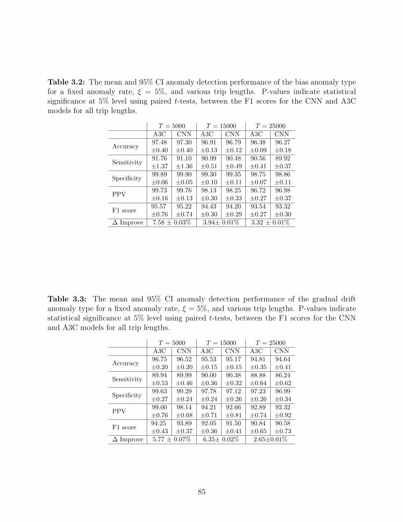
Table 3.2: The mean and 95% CI anomaly detection performance of the bias anomaly typefor a fixed anomaly rate, ξ = 5%, and various trip lengths. P-values indicate statisticalsignificance at 5% level using paired t-tests, between the F1 scores for the CNN and A3Cmodels for all trip lengths.
T = 5000 T = 15000 T = 25000A3C CNN A3C CNN A3C CNN
Accuracy97.48±0.40
97.30±0.40
96.91±0.13
96.79±0.12
96.38±0.09
96.27±0.18
Sensitivity91.76±1.37
91.10±1.36
90.99±0.51
90.48±0.49
90.56±0.41
89.92±0.37
Specificity99.89±0.06
99.90±0.05
99.30±0.10
99.35±0.11
98.75±0.07
98.86±0.11
PPV99.73±0.16
99.76±0.13
98.13±0.30
98.25±0.33
96.72±0.27
96.98±0.37
F1 score95.57±0.76
95.22±0.74
94.43±0.30
94.20±0.29
93.54±0.27
93.32±0.30
∆ Improve 7.58 ± 0.03% 3.94± 0.01% 3.32 ± 0.01%
Table 3.3: The mean and 95% CI anomaly detection performance of the gradual driftanomaly type for a fixed anomaly rate, ξ = 5%, and various trip lengths. P-values indicatestatistical significance at 5% level using paired t-tests, between the F1 scores for the CNNand A3C models for all trip lengths.
T = 5000 T = 15000 T = 25000A3C CNN A3C CNN A3C CNN
Accuracy96.75±0.20
96.52±0.20
95.53±0.15
95.17±0.15
94.81±0.35
94.64±0.41
Sensitivity89.94±0.53
89.99±0.46
90.00±0.36
90.38±0.32
88.88±0.64
86.24±0.62
Specificity99.63±0.27
99.29±0.24
97.78±0.24
97.12±0.26
97.23±0.26
96.99±0.34
PPV99.00±0.76
98.14±0.68
94.21±0.71
92.66±0.81
92.89±0.74
92.32±0.92
F1 score94.25±0.43
93.89±0.37
92.05±0.36
91.50±0.41
90.84±0.65
90.58±0.73
∆ Improve 5.77 ± 0.07% 6.35± 0.02% 2.65±0.01%
85
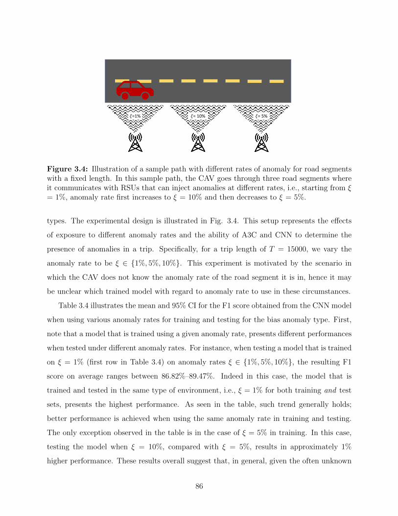
!=1% != 5%!= 10%
Figure 3.4: Illustration of a sample path with different rates of anomaly for road segmentswith a fixed length. In this sample path, the CAV goes through three road segments whereit communicates with RSUs that can inject anomalies at different rates, i.e., starting from ξ= 1%, anomaly rate first increases to ξ = 10% and then decreases to ξ = 5%.
types. The experimental design is illustrated in Fig. 3.4. This setup represents the effects
of exposure to different anomaly rates and the ability of A3C and CNN to determine the
presence of anomalies in a trip. Specifically, for a trip length of T = 15000, we vary the
anomaly rate to be ξ ∈ {1%, 5%, 10%}. This experiment is motivated by the scenario in
which the CAV does not know the anomaly rate of the road segment it is in, hence it may
be unclear which trained model with regard to anomaly rate to use in these circumstances.
Table 3.4 illustrates the mean and 95% CI for the F1 score obtained from the CNN model
when using various anomaly rates for training and testing for the bias anomaly type. First,
note that a model that is trained using a given anomaly rate, presents different performances
when tested under different anomaly rates. For instance, when testing a model that is trained
on ξ = 1% (first row in Table 3.4) on anomaly rates ξ ∈ {1%, 5%, 10%}, the resulting F1
score on average ranges between 86.82%–89.47%. Indeed in this case, the model that is
trained and tested in the same type of environment, i.e., ξ = 1% for both training and test
sets, presents the highest performance. As seen in the table, such trend generally holds;
better performance is achieved when using the same anomaly rate in training and testing.
The only exception observed in the table is in the case of ξ = 5% in training. In this case,
testing the model when ξ = 10%, compared with ξ = 5%, results in approximately 1%
higher performance. These results overall suggest that, in general, given the often unknown
86

Table 3.4: The mean and 95% CI for F1 score of the CNN model, obtained for varioustraining and testing combinations of anomaly rate under bias anomaly type.
Anomaly rate in testingξ = 1% ξ = 5% ξ = 10%
Anomalyrate intraining
ξ = 1% 89.47 ± 1.54 87.94 ± 0.74 86.82 ± 0.55ξ = 5% 92.01 ± 0.88 94.20 ± 0.29 95.53 ± 0.25ξ = 10% 67.08 ± 1.71 89.93 ± 0.50 94.54 ± 0.55
Table 3.5: The mean and 95% CI for F1 score of the CNN model, obtained for varioustraining and testing combinations of anomaly rate under gradual drift anomaly type.
Anomaly rate in testingξ = 1% ξ = 5% ξ = 10%
Anomalyrate intraining
ξ = 1% 87.20 ± 0.96 88.14 ± 0.61 89.00 ± 0.33ξ = 5% 77.59 ± 0.81 91.50 ± 0.41 94.21 ± 0.17ξ = 10% 86.35 ± 0.59 93.83 ± 0.19 95.31 ± 0.16
circumstances in which a previously trained model may be used, measures (such as dynamic
thresholding) may need to be taken to achieve the pre-trained algorithm’s full potential.
Similar results are seen under the gradual drift anomaly type, presented in Table 3.5.
In the remainder of this section, we use the average anomaly rate of ξ = 5% to train the
CNN model. This is consistent with real-world conditions where a single trained model is
often implemented, without the knowledge on the true anomaly rate to be experienced by
the CAVs.
Table 3.6 illustrates the anomaly detection performance of the models for the bias
anomaly type for trip length T = 15000, and anomaly rate ξ ∈ {1%, 5%, 10%}. From
the results, it is seen that the addition of the A3C model improves the performance of the
CNN model across all anomaly rates, particularly for F1 score. Specifically, paired t-tests
indicate a statistically significant difference at a 5% level in F1 score between the A3C and
CNN models for an anomaly rate of 5% and 10%. For the 1% anomaly rate, a statistical
difference is not obtained which is, in part, due to the few anomalies encountered by the
models. However, a better sensitivity and F1 score is still apparent from the results for the
A3C model.
Similarly, Table 3.7 illustrates the anomaly detection performance of the models for the
gradual drift anamaly type for trip length T = 15000, and anomaly rate ξ ∈ {1%, 5%, 10%}.
From the results, considering F1 score, it is seen that the addition of the A3C model improves
87
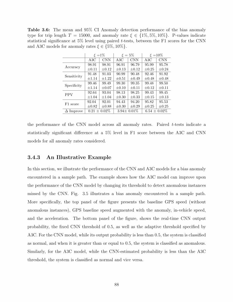
Table 3.6: The mean and 95% CI Anomaly detection performance of the bias anomalytype for trip length T = 15000, and anomaly rate ξ ∈ {1%, 5%, 10%}. P-values indicatestatistical significance at 5% level using paired t-tests, between the F1 scores for the CNNand A3C models for anomaly rates ξ ∈ {5%, 10%}.
ξ =1% ξ = 5% ξ =10%A3C CNN A3C CNN A3C CNN
Accuracy98.91±0.11
98.91±0.12
96.91±0.13
96.79±0.12
95.99±0.25
95.78±0.24
Sensitivity91.48±1.14
91.03±1.22
90.99±0.51
90.48±0.49
92.46±0.48
91.92±0.48
Specificity99.46±1.14
99.49±0.07
99.30±0.10
99.35±0.11
99.48±0.12
99.50±0.11
PPV92.64±1.04
93.04±1.04
98.13±0.30
98.25±0.33
99.43±0.15
99.45±0.13
F1 score92.04±0.82
92.01±0.88
94.43±0.30
94.20±0.29
95.82±0.25
95.53±0.25
∆ Improve 0.21 ± 0.02% 3.94± 0.01% 6.54 ± 0.02%
the performance of the CNN model across all anomaly rates. Paired t-tests indicate a
statistically significant difference at a 5% level in F1 score between the A3C and CNN
models for all anomaly rates considered.
3.4.3 An Illustrative Example
In this section, we illustrate the performance of the CNN and A3C models for a bias anomaly
encountered in a sample path. The example shows how the A3C model can improve upon
the performance of the CNN model by changing its threshold to detect anomalous instances
missed by the CNN. Fig. 3.5 illustrates a bias anomaly encountered in a sample path.
More specifically, the top panel of the figure presents the baseline GPS speed (without
anomalous instances), GPS baseline speed augmented with the anomaly, in-vehicle speed,
and the acceleration. The bottom panel of the figure, shows the real-time CNN output
probability, the fixed CNN threshold of 0.5, as well as the adaptive threshold specified by
A3C. For the CNN model, while its output probability is less than 0.5, the system is classified
as normal, and when it is greater than or equal to 0.5, the system is classified as anomalous.
Similarly, for the A3C model, while the CNN-estimated probability is less than the A3C
threshold, the system is classified as normal and vice versa.
88
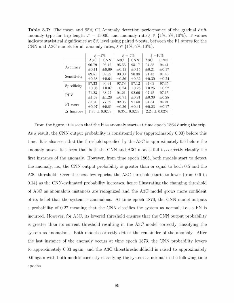
Table 3.7: The mean and 95% CI Anomaly detection performance of the gradual driftanomaly type for trip length T = 15000, and anomaly rate ξ ∈ {1%, 5%, 10%}. P-valuesindicate statistical significance at 5% level using paired t-tests, between the F1 scores for theCNN and A3C models for all anomaly rates, ξ ∈ {1%, 5%, 10%}.
ξ =1% ξ = 5% ξ =10%A3C CNN A3C CNN A3C CNN
Accuracy96.79±0.11
96.42±0.09
95.53±0.15
95.17±0.15
94.55±0.21
94.41±0.17
Sensitivity89.51±0.68
89.89±0.64
90.00±0.36
90.38±0.32
91.43±0.30
91.46±0.24
Specificity97.33±0.08
96.91±0.07
97.78±0.24
97.12±0.26
97.63±0.25
97.35±0.22
PPV71.23±1.38
68.27±1.28
94.21±0.71
92.66±0.81
97.45±0.30
97.15±0.28
F1 score79.34±0.97
77.59±0.81
92.05±0.36
91.50±0.41
94.34±0.23
94.21±0.17
∆ Improve 7.83 ± 0.02% 6.35± 0.02% 2.24 ± 0.02%
From the figure, it is seen that the bias anomaly starts at time epoch 1864 during the trip.
As a result, the CNN output probability is consistently low (approximately 0.03) before this
time. It is also seen that the threshold specified by the A3C is approximately 0.6 before the
anomaly onset. It is seen that both the CNN and A3C models fail to correctly classify the
first instance of the anomaly. However, from time epoch 1865, both models start to detect
the anomaly, i.e., the CNN output probability is greater than or equal to both 0.5 and the
A3C threshold. Over the next few epochs, the A3C threshold starts to lower (from 0.6 to
0.14) as the CNN-estimated probability increases, hence illustrating the changing threshold
of A3C as anomalous instances are recognized and the A3C model grows more confident
of its belief that the system is anomalous. At time epoch 1870, the CNN model outputs
a probability of 0.27 meaning that the CNN classifies the system as normal, i.e., a FN is
incurred. However, for A3C, its lowered threshold ensures that the CNN output probability
is greater than its current threshold resulting in the A3C model correctly classifying the
system as anomalous. Both models correctly detect the remainder of the anomaly. After
the last instance of the anomaly occurs at time epoch 1873, the CNN probability lowers
to approximately 0.03 again, and the A3C thresthreshouldhold is raised to approximately
0.6 again with both models correctly classifying the system as normal in the following time
epochs.
89
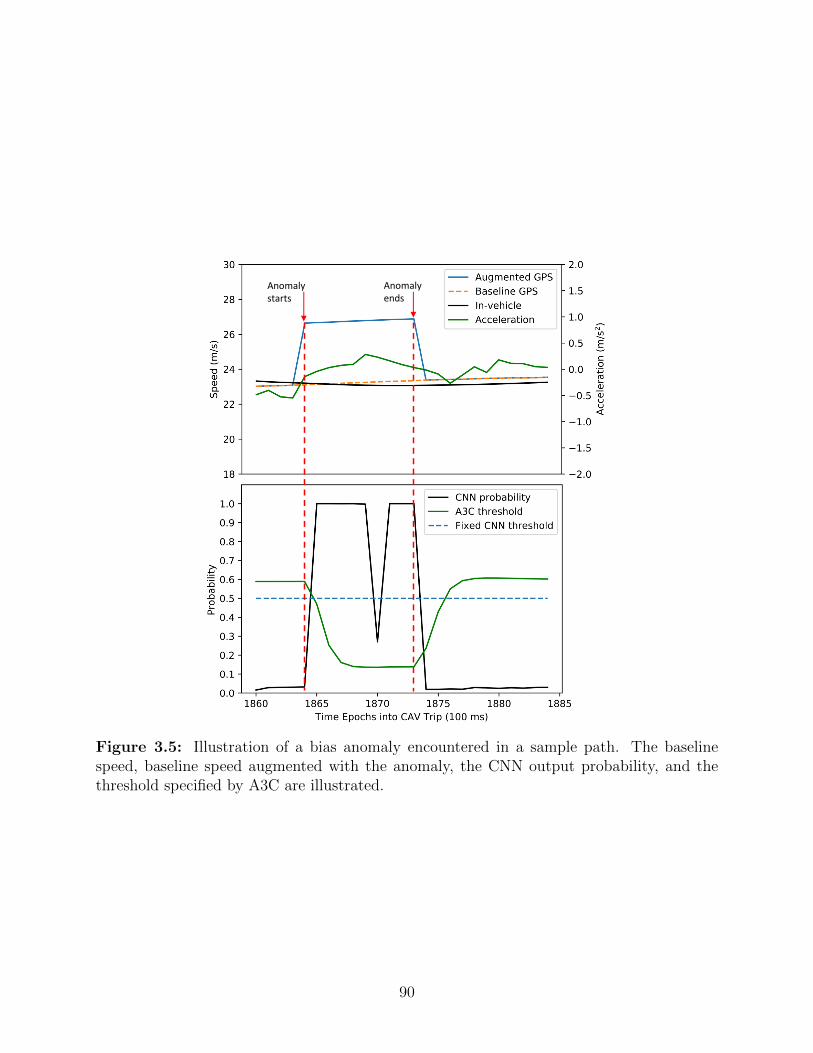
Anomaly starts
Anomaly ends
Figure 3.5: Illustration of a bias anomaly encountered in a sample path. The baselinespeed, baseline speed augmented with the anomaly, the CNN output probability, and thethreshold specified by A3C are illustrated.
90
3.5 Conclusion
The goal of this study is to develop a framework to detect anomalous behaviors in CAVs.
Specifically, we develop an approach that embeds a CNN classification model into a Bayesian
framework with the main objective of improving the performance of the primary classification
model. It should be noted that any classification model can be used as part of the framework.
The Bayesian framework consists of a POMDP model which is solved using the A3C
algorithm. In addition, we incorporate recent trip information to more actively react to
environmental changes and anomaly rates during a trip. The framework is also flexible to
use in other applications where the cost of false negatives/positives can be adjusted as needed
for specific purposes.
Our results show that the addition of the POMDP model leads to an improved
performance, especially with respect to F1 score. Specifically, we conduct experiments where
we fix the anomaly rate and vary the trip length and vice versa. In general, paired t-tests
illustrate a statistical significant improvement for the A3C model compared to the CNN
model’s performance. This research contributes to the field of ITS safety. Specifically, the
proposed framework addresses the issue of using a single trained classification model to detect
anomalies. In real-world conditions, the anomaly rate of road segments are not known in
advance. Hence, as illustrated in this study, using a hierarchical decision model may improve
the anomaly detection capabilities of the primary classification model.
The study is subject to certain limitations. In our experiments, similar to previous studies
in the literature, the anomalous instances in the speed sensor data are simulated. In our
experiments, to illustrate the capabilities of the framework, anomaly types are limited to
bias and gradual drift. Additional testing is required for other anomaly types and sensor
types. It is envisioned that data collected from recently completed and ongoing pilot studies
may contribute to the availability of real-world data including anomalous instances.
In future work, it may be useful to test additional models as the primary classification
model in the framework. Also, other deep reinforcement learning techniques can be used to
solve the POMDP model to compare to the performance of the A3C algorithm. In addition,
it may be interesting to use the stream of belief probabilities generated by the POMDP in
91

real-time as an input to an additional decision making model to more accurately approximate
the true state of the system.
92
Conclusion
In this research, we investigate the several aspect of CAVs under cyber-security and safety
uncertainties. Specifically, in Chaper 1, we investigate real-time sensor anomaly detection
and identification in CAVs. We develop a robust anomaly detection approach through
combining a deep learning method, namely convolutional neural network (CNN), with a well-
established anomaly detection method, Kalman filtering, to detect and identify anomalous
behavior in CAVs in real-time. Our numerical experiments demonstrate that the developed
approach can detect anomalies and identify their sources with high accuracy, sensitivity, and
F1 score.
In Chapter 2, we focus on the limitations of semi-autonomous vehicles under certain
circumstances where it is safer for the human driver to be in control compared to the
automated driving system. We investigate the transfer of control authority in semi-
autonomous vehicles to improve overall road safety. We develop a Markov decision process
(MDP) model to prescribe the entity in charge to minimize the expected safety risk of a
trip. We also develop a partially observable Markov decision process (POMDP) model to
account for cases when only partial information of the environmental risk is available. We
gain insights into the associated risks and advantages of authority control transitions for
semi-autonomous vehicles in certain conditions.
In Chapter 3 we investigate real-time dynamic thresholding in classification algorithms to
adapt to complex road and environmental conditions. Traditional classification algorithms
use fixed and a priori determined thresholds which determine if information is anomalous or
not. However, this approach does not allow for incorporating feedback obtained during
a trip on the performance of the classification algorithm which may result in excessive
false positive/negatives. To address this problem, we develop a mathematical framework in
93

which we pair an anomaly classification algorithm, based on CNN, with a POMDP model to
determine the optimal dynamic threshold of an anomaly classification algorithm to maximize
the safety of a trip. The numerical experiments suggest that the addition of the POMDP
model improves the anomaly detection performance of the CNN model, resulting in high
accuracy, sensitivity, and positive predictive value. As a result, we gain insights into the
associated benefits and disadvantages of implementing a dynamic classification threshold in
response to complex exogenous factors.
94

Bibliography
95
Abadi, M., Barham, P., Chen, J., Chen, Z., Davis, A., Dean, J., Devin, M., Ghemawat, S.,
Irving, G., Isard, M., et al. (2016). Tensorflow: A system for large-scale machine learning.
In 12th Symposium on Operating Systems Design and Implementation, pages 265–283. 80
Ahmed, M., Mahmood, A. N., and Hu, J. (2016). A survey of network anomaly detection
techniques. Journal of Network and Computer Applications, 60:19–31. 72
Arad, J., Housh, M., Perelman, L., and Ostfeld, A. (2013). A dynamic thresholds scheme for
contaminant event detection in water distribution systems. Water research, 47(5):1899–
1908. 73
Bai, F., Stancil, D. D., and Krishnan, H. (2010). Toward understanding characteristics of
dedicated short range communications (dsrc) from a perspective of vehicular network
engineers. In Proceedings of the sixteenth annual international conference on Mobile
computing and networking, pages 329–340. ACM. 8
Belletti, F., Haziza, D., Gomes, G., and Bayen, A. M. (2017). Expert level control of
ramp metering based on multi-task deep reinforcement learning. IEEE Transactions on
Intelligent Transportation Systems, 19(4):1198–1207. 74
Bezemskij, A., Loukas, G., Gan, D., and Anthony, R. J. (2017). Detecting cyber-physical
threats in an autonomous robotic vehicle using bayesian networks. In Internet of Things
(iThings) and IEEE Green Computing and Communications (GreenCom) and IEEE
Cyber, Physical and Social Computing (CPSCom) and IEEE Smart Data (SmartData),
2017 IEEE International Conference on, pages 98–103. IEEE. 10, 109
Bezzina, D. and Sayer, J. (2014). Safety pilot model deployment: Test conductor team
report. Report No. DOT HS, 812:171. 18, 81
Bhuyan, M. H., Bhattacharyya, D. K., and Kalita, J. K. (2014). Network anomaly detection:
methods, systems and tools. Ieee communications surveys & tutorials, 16(1):303–336. 11
Campbell, J. L., Brown, J. L., Graving, J. S.and Richard, C. M., Lichty, M. G.and Bacon,
L. P., and Sanquist, T. (2018). Human factors design guidance for level 2 and level 3
automated driving concepts. 37
96
Chandola, V., Banerjee, A., and Kumar, V. (2009). Anomaly detection: A survey. ACM
computing surveys (CSUR), 41(3):15. 72
Chawla, N. V., Japkowicz, N., and Kotcz, A. (2004). Special issue on learning from
imbalanced data sets. ACM Sigkdd Explorations Newsletter, 6(1):1–6. 31
Checkoway, S., McCoy, D., Kantor, B., Anderson, D., Shacham, H., Savage, S., Koscher, K.,
Czeskis, A., Roesner, F., Kohno, T., et al. (2011). Comprehensive experimental analyses
of automotive attack surfaces. In USENIX Security Symposium. San Francisco. 8, 9, 109
Christiansen, P., Nielsen, L. N., Steen, K. A., Jørgensen, R. N., and Karstoft, H.
(2016). Deepanomaly: Combining background subtraction and deep learning for detecting
obstacles and anomalies in an agricultural field. Sensors, 16(11):1904. 10, 109
Currie, R. (2015). Developments in car hacking. SANS Institute, InfoSec Reading Room,
Accepted Dec, 5:33. 19
Curtis, S. (2015). Self-driving cars can be hacked using a laser pointer. The Telegraph, Sept,
8. 72
Darms, M., Rybski, P., and Urmson, C. (2008). Classification and tracking of dynamic
objects with multiple sensors for autonomous driving in urban environments. In Intelligent
Vehicles Symposium, 2008 IEEE, pages 1197–1202. IEEE. 9
Davies, A. (2015). Ford’s skipping the trickiest thing about self-driving cars. [Online;
accessed 7/17/2017]. 39
de La Bourdonnaye, F., Teuliere, C., Chateau, T., and Triesch, J. (2017). Learning of
binocular fixations using anomaly detection with deep reinforcement learning. In 2017
International Joint Conference on Neural Networks (IJCNN), pages 760–767. IEEE. 74
De Winter, J. C., Happee, R., Martens, M. H., and Stanton, N. A. (2014). Effects of adaptive
cruise control and highly automated driving on workload and situation awareness: A
review of the empirical evidence. Transportation research part F: traffic psychology and
behaviour, 27:196–217. 39
97
Eriksson, A. and Stanton, N. A. (2017). Takeover time in highly automated vehicles:
Noncritical transitions to and from manual control. Human factors, 59(4):689–705. 40
Fagnant, D. J. and Kockelman, K. (2015). Preparing a nation for autonomous vehicles:
opportunities, barriers and policy recommendations. Transportation Research Part A:
Policy and Practice, 77:167–181. 37
Field, M. (2017). Graffiti on stop signs could trick driverless cars into driving dangerously.
[Online; accessed 09-01-2017]. 8, 72
Foo, G. H. B., Zhang, X., and Vilathgamuwa, D. M. (2013). A sensor fault detection and
isolation method in interior permanent-magnet synchronous motor drives based on an
extended kalman filter. IEEE Transactions on Industrial Electronics, 60(8):3485–3495. 10
Goodrich, M. A. and Boer, E. R. (2000). Designing human-centered automation: Trade-offs
in collision avoidance system design. IEEE Transactions on Intelligent Transportation
Systems, 1(1):40–54. 38
Green, M. (2000). How long does it take to stop? Methodological analysis of driver
perception-brake times. Transportation Human Factors, 2(3):195–216. 39
Greenberg, A. (2015). Hackers remotely kill a jeep on the highwaywith me in it. Wired, 7:21.
7, 8
Gu, S., Lillicrap, T., Sutskever, I., and Levine, S. (2016). Continuous deep q-learning with
model-based acceleration. In International Conference on Machine Learning, pages 2829–
2838. 48
Guler, S. I., Menendez, M., and Meier, L. (2014). Using connected vehicle technology
to improve the efficiency of intersections. Transportation Research Part C: Emerging
Technologies, 46:121–131. 37
Huang, C., Wu, Y., Zuo, Y., Pei, K., and Min, G. (2018). Towards experienced anomaly
detector through reinforcement learning. In Thirty-Second AAAI Conference on Artificial
Intelligence. 74
98
Huq, N., Vosseler, R., and Swimmer, M. (2017). Cyberattacks against intelligent
transportation systems. Technical report, TrendLabs, Tech. Rep., 2017, available at
https://documents. trendmicro. com . 8
Ide, T. and Kashima, H. (2004). Eigenspace-based anomaly detection in computer
systems. In Proceedings of the tenth ACM SIGKDD international conference on Knowledge
discovery and data mining, pages 440–449. ACM. 73
Jo, M., Park, J., Baek, Y., Ivanov, R., Weimer, J., Son, S. H., and Lee, I. (2016). Adaptive
transient fault model for sensor attack detection. In Cyber-Physical Systems, Networks,
and Applications (CPSNA), 2016 IEEE 4th International Conference on, pages 59–65.
IEEE. 8, 109
Kaber, D. B. and Endsley, M. R. (2004). The effects of level of automation and adaptive
automation on human performance, situation awareness and workload in a dynamic control
task. Theoretical Issues in Ergonomics Science, 5(2):113–153. 39
Kalman, R. E. (1960). A new approach to linear filtering and prediction problems. Journal
of basic Engineering, 82(1):35–45. 10
Kalmuk, A., Granichin, O., Granichina, O., and Ding, M. (2016). A dynamic threshold based
algorithm for change detection in autonomous systems. IFAC-PapersOnLine, 49(13):141–
145. 73
Kang, M.-J. and Kang, J.-W. (2016). Intrusion detection system using deep neural network
for in-vehicle network security. PloS one, 11(6):e0155781. 10, 109
Khalastchi, E., Kaminka, G. A., Kalech, M., and Lin, R. (2011). Online anomaly detection
in unmanned vehicles. In The 10th International Conference on Autonomous Agents and
Multiagent Systems-Volume 1, pages 115–122. International Foundation for Autonomous
Agents and Multiagent Systems. 10, 109
Kingma, D. P. and Ba, J. (2014). Adam: A method for stochastic optimization. International
Conference on Learning Representations (ICLR), San Diego, USA. 17, 76
99
Koo, J., Shin, D., Steinert, M., and Leifer, L. (2016). Understanding driver responses to voice
alerts of autonomous car operations. International journal of vehicle design, 70(4):377–
392. 40
Koscher, K., Czeskis, A., Roesner, F., Patel, S., Kohno, T., Checkoway, S., McCoy, D.,
Kantor, B., Anderson, D., Shacham, H., et al. (2010). Experimental security analysis of
a modern automobile. In Security and Privacy (SP), 2010 IEEE Symposium on, pages
447–462. IEEE. 7, 8, 71, 109
Krizhevsky, A., Sutskever, I., and Hinton, G. (2012). Imagenet classification with deep
convolutional neural networks. Advances in neural information processing systems, pages
1097–1105. 16, 17
Kruegel, C., Mutz, D., Robertson, W., and Valeur, F. (2003). Bayesian event classification
for intrusion detection. In 19th Annual Computer Security Applications Conference, 2003.
Proceedings., pages 14–23. IEEE. 72
Kyriakidis, M., Happee, R., and de Winter, J. C. (2015). Public opinion on automated
driving: Results of an international questionnaire among 5000 respondents. Transportation
research part F: traffic psychology and behaviour, 32:127–140. 38
Lambert, F. (2017). Tesla autopilot crash caught on dashcam shows how not to use the
system. Accessed 6/17/2017. 38, 50
Levi, M., Allouche, Y., and Kontorovich, A. (2018). Advanced analytics for connected car
cybersecurity. In 2018 IEEE 87th Vehicular Technology Conference (VTC Spring), pages
1–7. IEEE. 109
Levine, S., Finn, C., Darrell, T., and Abbeel, P. (2016). End-to-end training of deep
visuomotor policies. The Journal of Machine Learning Research, 17(1):1334–1373. 74
Levy, H. (2015). Stochastic dominance: Investment decision making under uncertainty.
Springer. 57
100
Lillicrap, T. P., Hunt, J. J., Pritzel, A., Heess, N., Erez, T., Tassa, Y., Silver, D., and
Wierstra, D. (2015). Continuous control with deep reinforcement learning. arXiv preprint
arXiv:1509.02971. 74
Lin, R., Khalastchi, E., and Kaminka, G. A. (2010). Detecting anomalies in unmanned
vehicles using the mahalanobis distance. In Robotics and Automation (ICRA), 2010 IEEE
International Conference on, pages 3038–3044. IEEE. 10, 109
Litman, T. (2017). Autonomous vehicle implementation predictions. Victoria Transport
Policy Institute Victoria, Canada. 7
Loebis, D. B., Sutton, R., Chudley, J., and Naeem, W. (2004). Sensor faults: Detection
methods and prevalence in real-world datasets. Control engineering practice, 12(12):1531–
1539. 15
Lu, Z. and de Winter, J. C. (2015). A review and framework of control authority transitions
in automated driving. Procedia Manufacturing, 3:2510–2517. 38
Malhotra, P., Vig, L., Shroff, G., and Agarwal, P. (2015). Long short term memory networks
for anomaly detection in time series. In Proceedings, page 89. Presses universitaires de
Louvain. 13
Marchetti, M., Stabili, D., Guido, A., and Colajanni, M. (2016). Evaluation of anomaly
detection for in-vehicle networks through information-theoretic algorithms. In 2016
IEEE 2nd International Forum on Research and Technologies for Society and Industry
Leveraging a better tomorrow (RTSI), pages 1–6. IEEE. 109
Merat, N., Jamson, A. H., Lai, F. C., Daly, M., and Carsten, O. M. (2014a). Transition
to manual: Driver behaviour when resuming control from a highly automated vehicle.
Transportation research part F: traffic psychology and behaviour, 27:274–282. 40
Merat, N., Jamson, H. A., Lai, F., and Carsten, O. (2014b). Human factors of highly
automated driving: results from the easy and citymobil projects. In Road vehicle
automation, pages 113–125. Springer. 39
101
Meyer, G. and Beiker, S. (2014). Road Vehicle Automation. Springer. 7
Miller, D., Sun, A., Johns, M., Ive, H., Sirkin, D., Aich, S., and Ju, W. (2015). Distraction
becomes engagement in automated driving. In Proceedings of the Human Factors and
Ergonomics Society Annual Meeting, volume 59, pages 1676–1680. SAGE Publications
Sage CA: Los Angeles, CA. 40
Mnih, V., Badia, A. P., Mirza, M., Graves, A., Lillicrap, T., Harley, T., Silver, D., and
Kavukcuoglu, K. (2016). Asynchronous methods for deep reinforcement learning. In
International conference on machine learning, pages 1928–1937. 47, 64, 74, 79, 80
Mnih, V., Kavukcuoglu, K., Silver, D., Rusu, A. A., Veness, J., Bellemare, M. G., Graves,
A., Riedmiller, M., Fidjeland, A. K., Ostrovski, G., et al. (2015). Human-level control
through deep reinforcement learning. Nature, 518(7540):529. 74
Mo, Y., Garone, E., Casavola, A., and Sinopoli, B. (2010). False data injection attacks
against state estimation in wireless sensor networks. In Decision and Control (CDC),
2010 49th IEEE Conference on, pages 5967–5972. IEEE. 11
Moavenzadeh, J. and Lang, N. (2018). Reshaping urban mobility with autonomous vehicles
lessons from the city of boston. Technical report. 72
Mohamed, A. H. and Schwarz, K. P. (1999). Adaptive kalman filtering for ins/gps. In
Adaptive Kalman filtering for INS/GPS. 14
Muter, M. and Asaj, N. (2011). Entropy-based anomaly detection for in-vehicle networks.
In Intelligent Vehicles Symposium (IV), 2011 IEEE, pages 1110–1115. IEEE. 10, 109
National Safety Council (2015). Injury facts. 112
NHTSA (2013). Preliminary statement of policy concerning automated vehicles. National
Highway Traffic Safety Administration and others, Washington, DC, pages 1–14. 10, 71
Ni, D. (2015). Traffic flow theory: Characteristics, experimental methods, and numerical
techniques. Butterworth-Heinemann. 71
102
Parasuraman, R. and Manzey, D. H. (2010). Complacency and bias in human use of
automation: An attentional integration. Human factors, 52(3):381–410. 38
Park, J., Ivanov, R., Weimer, J., Pajic, M., and Lee, I. (2015). Sensor attack detection
in the presence of transient faults. In Proceedings of the ACM/IEEE Sixth International
Conference on Cyber-Physical Systems, pages 1–10. ACM. 10, 109
Park, S.-h., Kim, S.-m., and Ha, Y.-g. (2016). Highway traffic accident prediction using vds
big data analysis. The Journal of Supercomputing, 72(7):2815–2831. 31
Parkinson, S., Ward, P., Wilson, K., and Miller, J. (2017). Cyber threats facing autonomous
and connected vehicles: Future challenges. IEEE transactions on intelligent transportation
systems, 18(11):2898–2915. 71
Petit, J. and Shladover, S. E. (2015). Potential cyberattacks on automated vehicles. IEEE
Transactions on Intelligent Transportation Systems, 16(2):546–556. 8, 11, 19, 38, 71, 109
Pous, N., Gingras, D., and Gruyer, D. (2017). Intelligent vehicle embedded sensors
fault detection and isolation using analytical redundancy and nonlinear transformations.
Journal of Control Science and Engineering, 2017. 9
Puterman, M. (1994). Markov Decision Processes: Discrete Stochastic Dynamic
Programming. John Wiley and Sons, New York, NY. 49
Ran, B. and Boyce, D. (2012). Dynamic urban transportation network models: theory
and implications for intelligent vehicle-highway systems, volume 417. Springer Science
& Business Media. 7
Realpe, M., Vintimilla, B., and Vlacic, L. (2015). Sensor fault detection and diagnosis
for autonomous vehicles. In MATEC Web of Conferences, volume 30, page 04003. EDP
Sciences. 9
Rios-Torres, J. and Malikopoulos, A. A. (2016). A survey on the coordination of connected
and automated vehicles at intersections and merging at highway on-ramps. IEEE
Transactions on Intelligent Transportation Systems, 18(5):1066–1077. 71
103
Roy, N., Gordon, G., and Thrun, S. (2005). Finding approximate pomdp solutions through
belief compression. Journal of artificial intelligence research, 23:1–40. 74
Rudin-Brown, C. M. and Parker, H. A. (2004). Behavioural adaptation to adaptive cruise
control (acc): implications for preventive strategies. Transportation Research Part F:
Traffic Psychology and Behaviour, 7(2):59–76. 40
SAE (2014). Taxonomy and definitions for terms related to on-road motor vehicle automated
driving systems. SAE Standard J3016, pages 01–16. 38
SAE (2016). Taxonomy and definitions for terms related to driving automation systems for
on-road motor vehicles. 37
Schmidhuber, J. (2015). Deep learning in neural networks: An overview. Neural networks,
61:85–117. 10, 17
Sharma, A. B., Golubchik, L., and Govindan, R. (2010). Sensor faults: Detection methods
and prevalence in real-world datasets. ACM Transactions on Sensor Networks (TOSN),
6(3):23. 11
Singh, S. (2015). Critical reasons for crashes investigated in the national motor vehicle crash
causation survey. Technical report. 71
Srivastava, N., H. G. K. A. S. I. and Salakhutdinov, R. (2014). Dropout: a simple
way to prevent neural networks from overfitting. Journal of machine learning research,
15(1):1929–1958. 17
Strand, N., Nilsson, J., Karlsson, I. M., and Nilsson, L. (2014). Semi-automated versus highly
automated driving in critical situations caused by automation failures. Transportation
research part F: traffic psychology and behaviour, 27:218–228. 40
Sutton, R. S. and Barto, A. G. (2018). Reinforcement learning: An introduction. MIT press.
74
Taylor, A., Leblanc, S., and Japkowicz, N. (2016). Anomaly detection in automobile
control network data with long short-term memory networks. In 2016 IEEE International
104
Conference on Data Science and Advanced Analytics (DSAA), pages 130–139. IEEE. 10,
109
Tesla (2017). Tesla model s owner’s manual. Accessed 6/17/2017. 38
Tieleman, T. and Hinton, G. (2012). Lecture 6.5-rmsprop: Divide the gradient by a running
average of its recent magnitude. In COURSERA: Neural networks for machine learning.
80
Trippel, T., Weisse, O., Xu, W., Honeyman, P., and Fu, K. (2017). Walnut: Waging doubt
on the integrity of mems accelerometers with acoustic injection attacks. In Security and
Privacy (Euro S&P), 2017 IEEE European Symposium, pages 3–18. IEEE. 19
Truong, K. N., Patel, S. N., Summet, J. W., and Abowd, G. D. (2005). Preventing camera
recording by designing a capture-resistant environment. In International Conference on
Ubiquitous Computing, pages 73–86. Springer. 8
USDOT (2016). United states department of transportation. connected vehicles and cyber
security. [Online; accessed 09-03-2017]. 7
Van Hasselt, H., Guez, A., and Silver, D. (2016). Deep reinforcement learning with double
q-learning. In Thirtieth AAAI Conference on Artificial Intelligence. 48, 79
van Wyk, F., Wang, Y., Khojandi, A., and Masoud, N. (2019). Real-time sensor anomaly
detection and identification in automated vehicles. IEEE Transactions on Intelligent
Transportation Systems. 75, 76, 81
Wei, X., Verhaegen, M., and van Engelen, T. (2010). Sensor fault detection and isolation for
wind turbines based on subspace identification and kalman filter techniques. International
Journal of Adaptive Control and Signal Processing, 24(8):687–707. 10
Weimerskirch, A. and Gaynier, R. (2015). An overview of automotive cybersecurity:
Challenges and solution approaches. In TrustED@ CCS, page 53. 7, 8, 71
105
Williams, C. (2017). Hackers hit d.c. police closed-circuit camera network, city officials
disclose. Technical report, Available at:https://www.washingtonpost.com/local/public-
safety/hackers-hit-dcpolice- closed-circuit-camera-network-city-officials-disclose. 8
Yan, C., Xu, W., and Liu, J. (2016). Can you trust autonomous vehicles: Contactless attacks
against sensors of self-driving vehicle. DEF CON, 24. 8, 109
Yang, S., Liu, Z., Li, J., Wang, S., and Yang, F. (2016). Anomaly detection for internet
of vehicles: A trust management scheme with affinity propagation. Mobile Information
Systems, 2016. 10, 109
Young, M. S. and Stanton, N. A. (2007). Back to the future: Brake reaction times for manual
and automated vehicles. Ergonomics, 50(1):46–58. 39
106

Appendices
107

A Summary of Key Literature and Notation for Chap-
ter 1
108
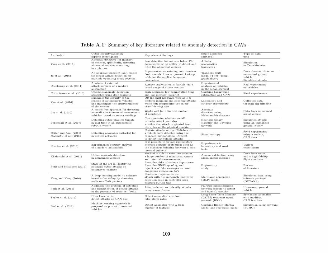
Table A.1: Summary of key literature related to anomaly detection in CAVs.
Author(s)Cyber-security/anomalyaspects investigated
Key relevant findingsStudy approach(method)
Type of dataused
Yang et al. (2016)
Anomaly detection for internetof vehicles, specifically, detectingabnormal vehicles operatingin a platoon
Low detection failure rate below 1%,demonstrating its ability to detect andfilter the abnormal vehicles
Affinitypropagationframework
Simulationin TransModeler
Jo et al. (2016)An adaptive transient fault modelfor sensor attack detection formultiple operating mode systems
Improvement on existing non-transientfault models. Uses a dynamic look-uptable for the applicable systemparameters
Transient faultmodel (TFM) usinggraph theory
Data obtained from anunmanned groundvehicle.Simulated attacks
Checkoway et al. (2011)Analysis of externalattack surfaces of a modernautomobile
Remote exploitation is feasible via abroad range of attack vectors
Experimentalanalyses on vehiclesin the sedan segment
Real experimentson vehicles
Christiansen et al. (2016)Obstacle/anomaly detectionalgorithm using deep learning
High accuracy, low computation timeand low memory footprint
Combine backgroundsubtraction and CNN
Field experiments
Yan et al. (2016)
Examines the security of thesensors of autonomous vehicles,and investigate the trustworthinessof the sensors
Off-the-shelf hardware were able toperform jamming and spoofing attackswhich can compromise the safetyof self-driving cars
Laboratory andoutdoor experiments
Collected datathrough experiments
Lin et al. (2010)A model-free approach for detectinganomalies in unmanned autonomousvehicles, based on sensor readings
Works well for a limited numberof attributes
Anomalydetection usingMahalanobis distance
Data from unmannedaerial vehicle
Bezemskij et al. (2017)Detecting cyber-physical threatsin real time in an autonomousrobotic vehicle
Can determine whether an AVis under attack and alsowhether the attack originated fromthe cyber or the physical domain
Heuristic binaryclassifier and Bayesiannetwork
Simulated attacksusing an unmannedground vehicle
Muter and Asaj (2011)Marchetti et al. (2016)
Detecting anomalies (attacks) forin-vehicle networks
Certain attacks on the CAN-bus ofa vehicle were detected using theproposed methodology. Difficultto detect low-volume attacks
Signal entropyField experimentsusing a vehicle,CAN data
Koscher et al. (2010)Experimental security analysisof a modern automobile
It is possible to bypass rudimentarynetwork security protections such asthe malicious bridging between a carsinternal subnets
Experiments inlaboratory and roadtests
Variousexperiments
Khalastchi et al. (2011)Online anomaly detectionin unmanned vehicles
Method is able to take into accounta large number of monitored sensorsand internal measurements
Anomaly detection usingMahalanobis distance
Data from robot,and a high-fidelityflight simulator
Petit and Shladover (2015)State of the art in identifyingpotential cyber attacks onautomated vehicles
Identifies risks of various importance.Identifies GNSS spoofing andinjection of fake messages as mostdangerous attacks on AVs
Exploratorystudy
Reviewof literature
Kang and Kang (2016)A deep learning model to enhancein-vehicular safety by detectingmalicious CAN packets
Real-time response to theattack with a significantly improveddetection ratio in controller areanetwork (CAN) bus
Multilayer perceptron(MLP) model
Simulated data usingsoftware package(OCTANE)
Park et al. (2015)Addresses the problem of detectionand identification of sensor attacksin the presence of transient faults
Able to detect and identify attacksusing sensor fusion
Pairwise inconsistenciesbetween sensors to detectand identify attacks
Unmanned groundvehicle
Taylor et al. (2016)Deep learning todetect attacks on CAN bus
Detect anomalies with lowfalse alarm rates
Long Short-Term Memory(LSTM) recurrent neuralnetwork (RNN)
Synthesize anomalieswith modifiedCAN bus data
Levi et al. (2018)Machine learning approach isproposed to protect connectedvehicles
Detect anomalies with a largenumber of features
Combine Hidden MarkovModel and regression model
Simulation using software(SUMO)
109109109

Table A.2: Summary of notation for Chapter 1.
Variable Descriptionn Number of sensorsα Anomaly ratex State variable of Kalman filterz Sensor measurementw Process noise of state-transition modelv Sensor measurement noiseν Innovation between measurement and predicted value of the measurementA State-transition matrixH Sensor measurement matrixR Process noise covariance matrixQ Measurement noise covariance matrix
R Process noise covariance matrix estimate
Q Measurement noise covariance matrix estimateS Covariance matrix of innovationP Error covariance matrix, where the error is the difference between true and predicted state valuesM Window size of adaptive Kalman filterγ χ2 detector parameter
110
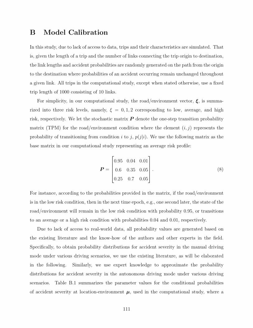
B Model Calibration
In this study, due to lack of access to data, trips and their characteristics are simulated. That
is, given the length of a trip and the number of links connecting the trip origin to destination,
the link lengths and accident probabilities are randomly generated on the path from the origin
to the destination where probabilities of an accident occurring remain unchanged throughout
a given link. All trips in the computational study, except when stated otherwise, use a fixed
trip length of 1000 consisting of 10 links.
For simplicity, in our computational study, the road/environment vector, ξ, is summa-
rized into three risk levels, namely, ξ = 0, 1, 2 corresponding to low, average, and high
risk, respectively. We let the stochastic matrix P denote the one-step transition probability
matrix (TPM) for the road/environment condition where the element (i, j) represents the
probability of transitioning from condition i to j, p(j|i). We use the following matrix as the
base matrix in our computational study representing an average risk profile:
P =
0.95 0.04 0.01
0.6 0.35 0.05
0.25 0.7 0.05
. (8)
For instance, according to the probabilities provided in the matrix, if the road/environment
is in the low risk condition, then in the next time epoch, e.g., one second later, the state of the
road/environment will remain in the low risk condition with probability 0.95, or transitions
to an average or a high risk condition with probabilities 0.04 and 0.01, respectively.
Due to lack of access to real-world data, all probability values are generated based on
the existing literature and the know-how of the authors and other experts in the field.
Specifically, to obtain probability distributions for accident severity in the manual driving
mode under various driving scenarios, we use the existing literature, as will be elaborated
in the following. Similarly, we use expert knowledge to approximate the probability
distributions for accident severity in the autonomous driving mode under various driving
scenarios. Table B.1 summarizes the parameter values for the conditional probabilities
of accident severity at location-environment µ, used in the computational study, where a
111
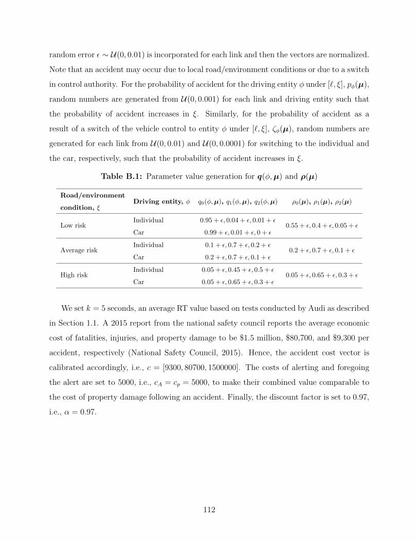
random error ε ∼ U(0, 0.01) is incorporated for each link and then the vectors are normalized.
Note that an accident may occur due to local road/environment conditions or due to a switch
in control authority. For the probability of accident for the driving entity φ under [`, ξ], pφ(µ),
random numbers are generated from U(0, 0.001) for each link and driving entity such that
the probability of accident increases in ξ. Similarly, for the probability of accident as a
result of a switch of the vehicle control to entity φ under [`, ξ], ζφ(µ), random numbers are
generated for each link from U(0, 0.01) and U(0, 0.0001) for switching to the individual and
the car, respectively, such that the probability of accident increases in ξ.
Table B.1: Parameter value generation for q(φ,µ) and ρ(µ)
Road/environment
condition, ξDriving entity, φ q0(φ,µ), q1(φ,µ), q2(φ,µ) ρ0(µ), ρ1(µ), ρ2(µ)
Low riskIndividual 0.95 + ε, 0.04 + ε, 0.01 + ε
0.55 + ε, 0.4 + ε, 0.05 + εCar 0.99 + ε, 0.01 + ε, 0 + ε
Average riskIndividual 0.1 + ε, 0.7 + ε, 0.2 + ε
0.2 + ε, 0.7 + ε, 0.1 + εCar 0.2 + ε, 0.7 + ε, 0.1 + ε
High riskIndividual 0.05 + ε, 0.45 + ε, 0.5 + ε
0.05 + ε, 0.65 + ε, 0.3 + εCar 0.05 + ε, 0.65 + ε, 0.3 + ε
We set k = 5 seconds, an average RT value based on tests conducted by Audi as described
in Section 1.1. A 2015 report from the national safety council reports the average economic
cost of fatalities, injuries, and property damage to be $1.5 million, $80,700, and $9,300 per
accident, respectively (National Safety Council, 2015). Hence, the accident cost vector is
calibrated accordingly, i.e., c = [9300, 80700, 1500000]. The costs of alerting and foregoing
the alert are set to 5000, i.e., cA = cp = 5000, to make their combined value comparable to
the cost of property damage following an accident. Finally, the discount factor is set to 0.97,
i.e., α = 0.97.
112
Vita
Franco van Wyk is from Upington, South Africa. He attended the Duineveld High School
in Upington and moved to Stellenbosch in 2011 to pursue a degree in engineering. He
received a Bachelor’s of Mechanical Engineering degree from the University of Stellenbosch
in 2014. He then received a Master’s degree in Engineering Management from the University
of Stellenbosch in 2016 where his research focused on decision-making in volatile business
environments. From there, he moved to Knoxville, Tennessee, to pursue a PhD in Industrial
Engineering at the University of Tennessee. He conducted research in the health care and
transportation sectors. His research in health care focused on the development of algorithms
to aid the early detection of sepsis, an illness caused by the body’s dysregulated response
to an infection. His research in transportation focused on improving the safety of connected
and automated vehicles under cyber-security and safety uncertainties.
113