Recent Developments and Future Perspectives in Nonlinear System Theory

Casti, J.L.

IIASA Working Paper

WP-80-123

August 1980

Casti, J.L. (1980) Recent Developments and Future Perspectives in Nonlinear System Theory. IIASA Working Paper. WP-

80-123 Copyright © 1980 by the author(s). http://pure.iiasa.ac.at/1346/

Working Papers on work of the International Institute for Applied Systems Analysis receive only limited review. Views or

opinions expressed herein do not necessarily represent those of the Institute, its National Member Organizations, or other

organizations supporting the work. All rights reserved. Permission to make digital or hard copies of all or part of this work

for personal or classroom use is granted without fee provided that copies are not made or distributed for profit or commercial

advantage. All copies must bear this notice and the full citation on the first page. For other purposes, to republish, to post on

servers or to redistribute to lists, permission must be sought by contacting repository@iiasa.ac.at

NOT FOR QUOTATION WITHOUT PERMISSION O F 'THE AUTHOR

RECENT DEVELOPMENTS AND FUTURE PERSPECTIVES I N NONLINEAR SYSTEM THEORY

John L . C a s t i

A u g u s t 1 9 8 0 WP-80 - 1 2 3

Working Papers are i n t e r i m reports on w o r k of t h e I n t e r n a t i o n a l I n s t i t u t e f o r A p p l i e d S y s t e m s A n a l y s i s and have received on ly l i m i t e d r e v i e w . V i e w s or op in ions expressed h e r e i n do no t necessari ly repre- s e n t those of t h e I n s t i t u t e o r of i t s N a t i o n a l M e m b e r O r g a n i z a t i o n s .

INTERNATIONAL I N S T I T U T E FOR A P P L I E D SYSTEMS ANALYSIS A - 2 3 6 1 L a x e n b u r g , A u s t r i a

PREFACE

Results on controllability, observability and realization of input/output data for linear systems are well-known and extensively covered in a variety of books and papers. What is not so well-known is that substantial progress has been made in recent years on providing similarly detailed results for nonlinear processes. This paper represents a survey of the most interesting work on nonlinear systems, together with a discussion of the major obstacles standing in the way of a comprehensive theory of nonlinear systems.

1. Basic Problems and Results in Linear System Theory

The theory of linear dynamical processes has by now been

developed to such an extent that it is only a slight exagger-

ation to term it a branch of applied mathematics, sharing equal

rank with more familiar areas such as hydrodynamics, classical

and quantum mechanics and electromagnetism, to name but a few.

For those who doubt this assessment of linear system theory,

a perusal of some of the more advanced recent literature [ I - 5 1

should prove to be an enlightening activity, showing how deeply

imbedded system-theoretic concepts are in areas such as algebraic

geometry, differential topology and Lie algebras. Conversely,

the "purer" parts of mathematics have proven to be fruitful

sources of inspiration for system theorists seeking more power-

ful tools with which to analyze and classify broad classes of

problems.

Encouraged by the tremendous success in the study of linear

processes, system theorists have been increasingly turning their

attention and methods to the analysis of the same circle of

questions for nonlinear systems. As one would suspect,

the jungleland of nonlinearity is not easily tamed and so far

no comprehensive theory has emerged capable of treating general

nonlinear processes with the detail available in the linear case.

Nonetheless, substantial progress has been made on several fronts

and part of our story will be to survey some of the more inter-

esting developments.

An equally important part of the picture we wish to present

is to outline some of the reasons why a complete theory of non-

linear systems seems remote, at least at our current level of

mathematical sophistication. All current indications point

toward the conclusion that seeking a completely general theory

of nonlinear systems is somewhat akin to the search for the Holy

Grail: a relatively harmless activity full of many pleasant sur-

prises and mild disappointments, but ultimately unrewarding. A

far more profitable path to follow is to concentrate upon special

classes of nonlinear problems, usually motivated by applica-

tions, and to use the structure inherent in these classes as

a guide to useful (i.e., applicable) results. As we go along

in this survey, we shall try to emphasize this approach by

example, as well as by precept.

Before entering into the mainstream of nonlinear system

theory and the problems inherent therein, let us briefly review

the principal questions and results of the linear theory. We

are concerned with a process described by the system of

differential equations

where x, u and y are n, m and p-dimensional vector functions,

taking values in the vector spaces X, U and Y, respectively.

For ease of exposition, we assume that the matrices F, G and H

are constant, although the theory extends easily to the time-

varying case at the expense of more delicate notation and

definitions.

The principal questions of mathematical system theory may

be conveniently separated into three categories:

A. ~eachability/Controllability -given an admissible

set of input functions R, what region a o f the system state

space X can be reached from the initial state xo in some pre-

scribed time T by application of inputs u E R. If x o # O and

2 = 0, then we have a problem of controllability; otherwise

it is a question of reachability. In the case of constant

F and G (the output matrix H plays no role in category A

problems), with !il = continuous functions on [O,Tl, the two

notions coincide and the basic result is

Theorem 1 [6-81. A state x is reachable (and controllable)

if and only if x is contained in the subspace of X generated by

the vectors

The system C is said to be completely reachable if and only if

s=x , i .e . , x IS reachable for every x E X . An immediate conse-

quence of Theorem 1 is

Corollary 1 . C is completely reachable if and only if the

n x nm matrix

has rank n.

Many variations on the above theme are possible by changing

R , 9 , T and/or admitting time-varying F and G (see [71 for de-

tails). However, the algebraic result given by Theorem 1 and

its corollary forms the cornerstone for the study of almost all

questions relating to reachability and controllability of linear

systems. As we shall see below, the same type of algebraic

result can also be obtained for large classes of nonlinear

systems at the expense of a more elaborate mathematical

machinery, further emphasizing the underlying algebraic nature

of dynamical systems.

B. Observability/Constructibi1ity- switching attention

from inputs to outputs, we consider the class of questions

centering upon what information can be deduced about the

system state from the measured output. As in category A,

the basic question comes in two forms, depending upon whether

we wish to determine the initial state x from knowledge of 0

future inputs and outputs (observability) or if we wish to

determine the current state x(T) from knowledge of past

inputs and outputs (constructibility) . The linearity of the

situation enables us to consider the case of no input (u= 0)

and, as in the controllability/reachability situation, the

two basic concepts of observability and constructibility

coincide if F and H are constant matrices. The main result

for category B questions is

Theorem 2 [ 6 -81 . A state x E X is unobservable (uncon-

structible) if and only if x is contained in the kernel of

the matrix

Note that the basic test implicit in Theorem 2 is given in

terms of unobservable states. Thus, any initial state x o # O

may be uniquely determined from the measured output y (t) ,

0 - < t - < T , T > 0, if and only if xo g! kernel O. The important

corollary to Theorem 2, characterizing complete observability/

constructibility is

Corollary 2. The system C is completely observable

(constructible) if and only if the matrix O has rank n.

The striking similarity in form between Theorems 1 and 2

suggests a duality between the concepts of reachability and

observability. This idea can be made mathematically precise

through the identifications

showing that any result concerning reachability may be tran-

scribed into a dual result about observability, and conversely.

C. Realizations/Identification -the basic questions

subsumed under categories A and B assume for their statement

that the system i.s given in the so-called state-variable

form C . The most important of all system-theoretic questions

is that of determining "good" state-variable models given only

input/output (experimental) data.

Consider the Laplace transform of the system C and let

W(s) and %(s) denote the transforms of the input and output

functions, respectively. It is then easy to see t h a t w a n d

g a r e linearly related as

where

is called the system transfer matrix. If W(s) is a strictly

proper rational matrix (i.e., the elements of W are ratios of

relatively prime polynomials with the degree of the numerator

less than that of the denominator), then we may expand W(*)

in a Laurent series about 00 obtaining

The matrix W (s) or, equivalently, the infinite sequence

{A,,A2,A3,...) will be called the input/output data (or

external description) of the system C . We can now state

the central problem of mathematical system theory:

The Realization Problem: given the input/output data

of a linear system C, determine a state-variable model C

such that

i) the input/output behavior of the model agrees

exactly with the given data and

ii) the model is completely reachable and completely

observable, i.e., the model is canonical.

Remark: Condition (ii), that the model be canonical,

is mathematically equivalent to requiring that the dimension

of the state space X of the model be minimal. However, for

purposes of extension to the nonlinear case, where X may not

even be a vector space, it is preferable to state the require-

ment as given above.

Perhaps surprisingly, the Realization Problem for linear

systems has the following definitive solution.

Theorem 3 [ 6 - 8 1 . For each input/output description of a

system there exists a canonical model 1, which is unique up

to a choice of coordinate syst&m in the state space X.

A weak form of the Realization Problem occurs when the

dimension of E is fixed in advance, perhaps by a priori

engineering or physical considerations, and only some of the

components of F, G and H need to be determined from the input/

output data. This is the so-called parameter identification

problem and is tantamount to not only forcing the system upon

the data (by fixing the dimension of X), but also partially

fixing the coordinate system in X (by demanding that certain

elements of F, G and H remain fixed). Nevertheless, much work

has been done on parameter estimation, especially in the case

where there are uncertainties in the data, a situation which

makes the conceptual approach somewhat easier to accept.

It will be noted that the Realization Problem demands - all

of the system input/output data before the internal model C

can be chosen. In principle, this involves an infinite data

string. Of somewhat more practical concern is the case in

which only a finite behavior sequence

is available. The construction of a canonical model C from N

the sequence B constitutes the partial realization problem, N

which has only recently been definitively resolved. While a

precise statement of the main result would take us too far

afield, the basic conclusion is that each behavior sequence

BN has a canonical realization Z which may be unique (modulo N'

a coordinate change in X), or which may contain a certain

number of undetermined parameters. Furthermore, it can be

shown that as N increases (more data becomes available), the

sequence of canonical realizations { C 1 is nested, i.e., the N

matrices F N'

GN, H of the realization C appear as submatrices N N'

k > 1. A complete discussion of these in the realization CN+k, -

matters is given in [9-101 .

In addition to the problems of categories A, B and C, two

other broad areas are also usually considered to form part of

the general field of mathematical system theory: stability

theory and optimization. Generations of work on optimal control

theory and stability is by now so well covered in the literature

that we shall refrain from a discussion of these areas here.

For the interested reader, the sources [11-131 can be recommended.

2. Linearization

Given a nonlinear internal model

the first temptation in analyzing questions of Type A or B is to

linearize the process (N) by choosing some nominal input u(t)

and generating the corresponding reference trajectory x(t).

Such a procedure yields the linearized dynamics

where

- - - z(t)=x(t) -x(t), v(t)=u(t) -u(t)r w(t)=y(t) -y(t),

with

with F ( . ) , G ( . ) and H ( . ) being evaluated at the pair (x (t) , u (t) ) . The approach to studying reachability/observability issues is

to now employ the time-varying analogues of Theorems 1 and 2

for the analysis of the system ZL. We would clearly like to

be able to conclude something about the c~ntrollability prop- - -

erties of (N) in a neighborhood of (x,u) by studying the

corresponding properties of C L' A typical result in this

direction is

1 Theorem 4 [ I 4 1 . Let the dynamics f (x,u) be C in a - -

neighborhood U of (x,u) . Then the system (N) is locally

controllable if the pair (F(t) ,G(t)) is controllable in U.

Here "local controllability" means that for each x* in some

neighborhood of 2, there exists a piecewise-continuous control

u* (t) , in some neighborhood of u(t), 0 - < t - < TI such that x (T) = 0.

The problem with the above linearized results is that they

usually provide only sufficient conditions and are inherently

local in character. As illustration of this point, consider

the 2nd-order nonlinear problem

- with 1 u (t) I 2 1. Let x(t) = 0, u (t) = 0, so that the linearized

system is

with

The pair ( F I G ) is not controllable since

Nevertheless, it can be shown [14] that each initial state

0 (xl ,x:) near (0.0) can be transferred to the origin in finite

time by a control of the above type. Thus, the system is

locally controllable although the linearized approximation is

not controllable.

Another obvious defect of linearization is the smoothness

requirement on the dynamics f(x,u) and/or the output function

h(x). In order for the linearization to make sense, these

functions must be at least continuously differentiable in each

argument. While many practical processes obey this restriction,

systems with switching points in the dynamics or other types

of discontinuities frequently occur and would be outside the

realm of straightforward linearization techniques.

3. Nonlinear Processes

The inadequacies of linearization as outlined in the

preceding section are far from the only reasons why we would

like to develop a system theory for truly nonlinear processes.

Some of the reasons are associated with intrinsic features of

nonlinear dynamical processes, while others are more closely

connected with the methods employed in the study of such pro-

cesses. Let us consider the first of these aspects as it is

somewhat more relevant to the issues raised in this survey.

Among the inherent difficulties associated with nonlinear

processes, which are not present in linear phenomena we may

cite nonuniqueness, singularities and critical dependence on

parameters as features worthy of special attention.

Nonuniqueness -the simple scalar process

illustrates the fact that a nonlinear process may have multiple

equilibria, even in the presence of no control input (u= 0).

In the event a feedback law

is employed, the closed-loop dynamics

may have an infinite (or even uncountable) number of equilibria,

depending upon the form of 4 . Clearly, this situation is in

stark contrast to the linear case where only the equilibrium

x = O can generically occur. Furthermore, no linearized version

of (1) can possibly capture the global structure of the system

equilibria manifold as a function of a and b.

Singularities -the solutions of many nonlinear systems

may develop singularities, even though the systems themselves

have smooth coefficients. The simple two-point boundary value

problem

possesses no solutions without singularities for any T > 0 .

In a more system-theoretic direction, it can be shown [ 1 5 ]

that the system

with lu(t)I - < E < < 1, has a reachable set from xo which is

homeomorphic to a disk for T small, but encircles the origin

for T large (see Fig. 1).

T smai l T l a r g e

F igu re 1 . The Reachable S e t f o r t h e System ( 2 )

The s i t u a t i o n can be even worse than t h i s a s some n o n l i n e a r

systems have a reachab le set which is n o t even simply-connected

[ 1 5 ] . I n t h e l i n e a r c a s e , o f course , Theorem 1 shows t h a t t h e

n reachab le set i s a subspace o f R , hence, n o t o n l y simply-

connected b u t even convex. Again, no l i n e a r i z e d v e r s i o n o f t h e

system ( 2 ) can hope t o c a p t u r e t h e g l o b a l s t r u c t u r e o f t h e

reachab le set .

The s imple b i l i n e a r system

a l s o shows t h a t a s t a t e may no t be reachab le from t h e o r i g i n

w i t h bounded c o n t r o l . Thus, a more a p p r o p r i a t e state space f o r

n t h i s problem i s t h e "punctured" reg ion R - ( 0 1 , r a t h e r t han

R" i t se l f . I n g e n e r a l , t h e " n a t u r a l " s t a t e space f o r a non-

l i n e a r p rocess i s no l onge r t h e f a m i l i a r v e c t o r space ( o r

module) o f t h e l i n e a r t heo ry , b u t a much more compl ica ted

mathemat ical o b j e c t , u s u a l l y some t ype o f mani fo ld i n a

Euc l idean space o f h igh dimension. For i n s t a n c e , i f t h e

system i s m u l t i l i n e a r t h e n t h e s t a t e space h a s t h e s t r u c t u r e

o f an a b e l i a n v a r i e t y (= a l g e b r a i c man i fo ld ) [161. Such f a c t s

account f o r t h e need t o employ much more s o p h i s t i c a t e d ma-

ch ine ry t han s imp le l i n e a r a l g e b r a t o s t u d y t h e s t r u c t u r e o f

n o n l i n e a r p rocesses .

C r i t i c a l Dependence on Parameters - f o r t h e l i n e a r dynamical

system

t h e r e a r e no pa rame t r i c changes i n t h e e lements o f F which can

cause t h e system t o have more t h a n a s i n g l e s o l u t i o n cu rve x ( t ) .

However, t h i s i s f a r from t h e c a s e f o r n o n l i n e a r p rocesses . For

example, c o n s i d e r t h e sys tem

For X > ( a c e r t a i n p o s i t i v e number), t h e sys tem has no smooth

s o l u t i o n . For X = f3 t h e r e is e x a c t l y one smooth s o l u t i o n ,

wh i l e f o r 0 < X < B t h e r e a r e two s o l u t i o n s . Thus, f3 i s a b i f u r -

c a t i o n p o i n t i n t h e parameter space a t which t h e c h a r a c t e r o f

t h e s o l u t i o n set changes r a d i c a l l y .

To i l l u s t r a t e ano the r p o i n t , c o n s i d e r t h e sys tem

For each p , -1 - < p 2 0 , a l l s o l u t i o n s t end a s y m p t o t i c a l l y t o z e r o

as t+m. As p crosses 0, the system has a unique periodic

solution p(p) and the origin becomes a source. For all p ,

0 < p 2 1 , every nontrivial solution tends to p (p) as t + . Thus, p = O is a bifurcation point at which the equilibrium

at the origin changes suddenly from a sink to a source and

a limit cycle p(p) is created. This so-called "Hopf bifur-

cation" is a consequence of the system nonlinearity and has

no counterpart in linear problems.

Finally, consider the equilibria of the nonlinear system

where a is an m-dimensional vector of parameters. The equi-

libria x* for which f (x*,a) = 0 depend upon a and we can define

a map

X : A - + X *

a H x (a)

where A c R ~ , x c R". Under appropriate hypotheses on the function

f, properties of the map X can be characterized using Thom's

theory of catastrophes. In particular, it is of interest to

categorize those submanifolds of A for which the map X is dis-

continuous, the so-called "catastrophe" manifold. Again, if

f is linear the map X is continuous and there is no interesting

structure to analyze. Thus, no linearized version of the problem

will suffice to study the geometry of the equilibrium manifold.

The above examples provide convincing evidence of the need

to develop a nonlinear system theory capable of handling the

same broad array of questions so successfully dealt with by the

linear theory. In succeeding sections, we present some steps

in this direction. As will become evident, almost everything

remains to be done to complete such a program despite the

impressive advances of recent years.

4. Reachability and Controllability

Smooth Systems

Certainly the area in which most progress has been made in

understanding the system-theoretic behavior of nonlinear processes

is in the effective characterization of reachable sets and in the

determination of algebraic criteria for complete reachability.

Since the mathematical apparatus involved goes somewhat beyond

the elementary linear algebra which suffices for the study of

linear systems, we make the following definitions as originally

given in [ 1 71 .

Consider the nonlinear system

where u E R c R ~ , x E M I a cm-connected manifold of dimension n

and f and h are cm functions of their arguments. To

simplify notation, it is assumed that M admits globally

defined coordinates x = (x l , ..., x,)', allowing us to identify

the points of M with their coordinate representations and to

describe the control system (N) in the usual engineering form

above. We also assume that (N) is complete, i.e., for every

bounded measurable control u(t) and every x E M , there exists 0

a solution of ;( = f (x,u) satisfying x(0) = x x(t) E M for all 0 ' real t.

~efinition 1. Given a point X*E MI we say that x* is

reachable from xo at T if there exists a bounded measurable

control u(t), satisfying u ( t ) ~ 5 2 , such that the system trajec-

tory satisfies x(0) = x x(T) = x*, x(t) E MI 0 < t < T. 0 ' - -

The set of states reachable from xo is denoted as

9(x0) = U {x : x reachable from x at time T) . O5T<m 0

We say (N) is reachable at x if R(xO) = M and reachable if - -0

g(x) = M for all x EM.

Since it may be necessary to either travel a long distance

or a great time to reach points near x the property of reach- 0 '

ability from xo is not always of practical use. This fact leads

to a local version of reachability.

Definition 2. (N) is locally reachable at x if for every - -0 neighborhood U of xo, R(x ) is also a neighborhood of x with 0 0

the trajectory from x toS(x ) lying entirely within U. The 0 0

system (N) is locally reachable if it is locally reachable for

every x E M.

The reachability concept detailed in Definition 1 is not

symmetric: x* may be reachable from xo but not conversely (in

contrast to the situation for autonomous linear systems). To

remedy this situation, we need a weaker notion of reachability.

This is provided by

~efinition 3. Two states x* and 2 are weakly reachable

0 1 from each other if and only if there exist states x ,x ,..., x

k

i O * = x and either x is reachable from x i- 1 such that x = x , x

i- 1 i or x is reachable from x , i =1,2, ..., k. The system ( N ) is

said to be weakly reachable if it is weakly reachable from every

x E M . Since weak reachability is a global concept like reach-

ability, we can define a local version of it in correspondence

to Definition 2.

Among the various reachability concepts, we have the

following chain of implications

locally reachable reachable

locally weakly reachable => weakly reachable

For autonomous linear systems it can be shown that all four of

the above notions coincide.

The advantage of local weak reachability over the other

concepts defined above is that it lends itself to a simple

algebraic test. For this, however, we need a few additional

notions.

Definition 4. Let p (x) , q (x) be two cm vector fields on

M. Then the Jacobi bracket of p and q, denoted [p,q] is given

by

The set of all cm vector fields on M is an infinite-dimensional

vector space denoted by X(M) and becomes a Lie algebra under the

the multiplication defined by the Jacobi bracket.

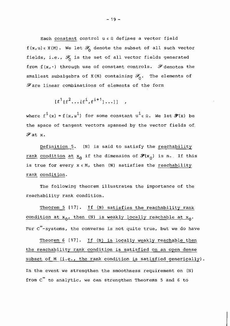
Each constant control u E Q defines a vector field

f (x,u) E X(M) . We let 9 denote the subset of all such vector 0

fields, i.e., 3$ is the set of all vector fields generated

from f(x,*) through use of constant controls. Tdenotes the

smallest subalgebra of X(M) containing So. The elements of

Fa re linear combinations of elements of the form

i i where fi(x) = f (x,u ) for some constant u E Q. We let P(x) be

the space of tangent vectors spanned by the vector fields of.

F a t x.

Definition 5. (N) is said to satisfy the reachability

rank condition at xo if the dimension of F(x0) is n.. If this -

is true for every x E M , then (N) satisfies the reachability

rank condition.

The following theorem illustrates the importance of the

reachability rank condition.

Theorem 5 [ 1 7 ] . If (N) satisfies the reachability rank

condition at xo, then (N) is weakly locally reachable at xo.

For ca-systems, the converse is not quite true, but we do have

Theorem 6 [ 1 7 1 . If (N) is locally weakly reachable then

the reachability rank condition is satisfied on an open dense

subset of M (i.e., the rank condition is satisfied generically).

In the event we strengthen the smoothness requirement on (N)

from C- to analytic, we can strengthen Theorems 5 and 6 to

Theorem 7 [I 71 . If (N) is analytic then (N) is weakly

reachable if and only if it is locally weakly reachable if

and only if the reachability rank condition is satisfied.

The simplest illustration of the use of these results is

to recapture the linear result of Theorem I. In this case

.F = {Fx + Gu: u E R ) 0

so the Lie algebra is generated by the vector fields

{Fx,gl,g2, ...,g ,I, where gi denotes the ith column of G

regarded as a constant vector field. Computing brackets

yields

2 [Fx. [Fxrgjll = gj I [gif [ F ~ , g ~ l l = 0 I etc.

The Cayley-Hamilton Theorem implies that ?is spanned by the

vector fields Fx and the constant vector fields Fig j r

= 0 1 , n - 1 , j = I 2 . . . m . Thus, in this context the

reachability rank condition reduces to the condition of

Theorem I, namely, (N) is locally reachable if and only if

2 n- 1 rank [G(FG(F G I . .. ( F GI = n .

However, for linear systems local reachability and reachability

are equivalent, so the usual results are obtained.

The practical problem with applying the preceding results

is that we have no nonlinear version of the Cayley-Hamilton

Theorem insuring that the test for complete reachability can

be concluded in a finite number of steps. In principle, we

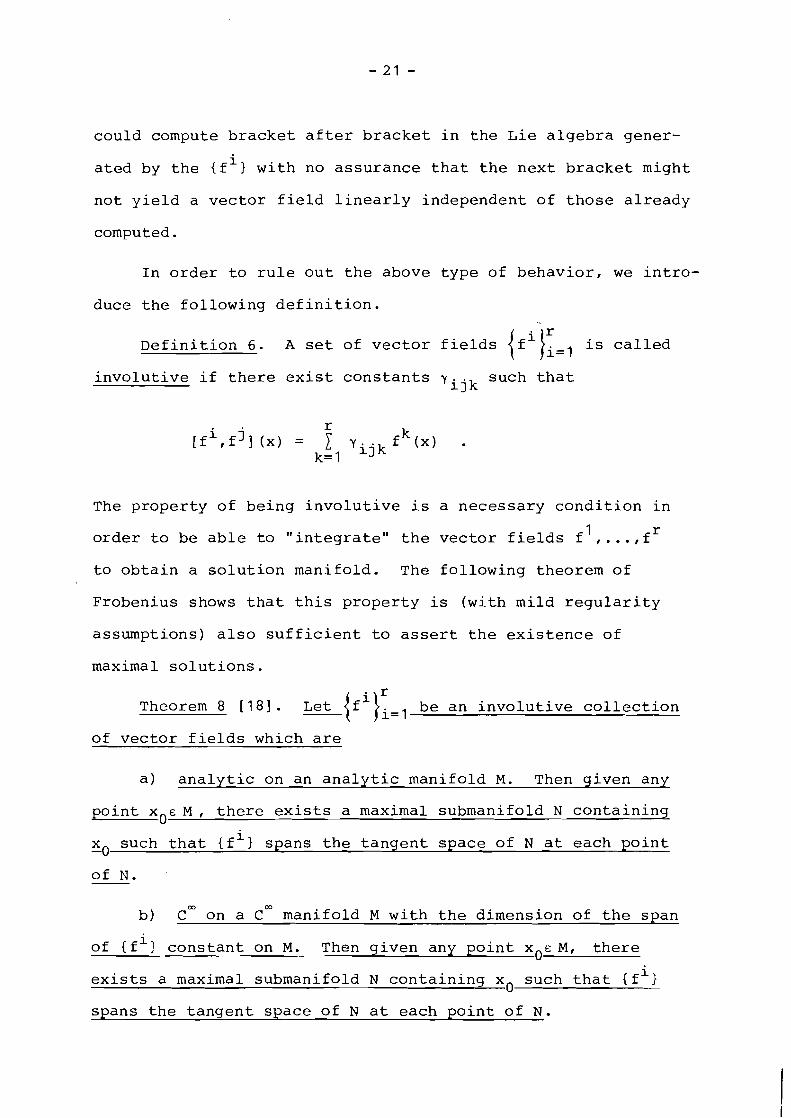
c o u l d compute b r a c k e t a f t e r b r a c k e t i n t h e L i e a l g e b r a gener -

a t e d by t h e i f i } w i t h no a s s u r a n c e t h a t t h e n e x t b r a c k e t m igh t

n o t y i e l d a v e c t o r f i e l d l i n e a r l y i n d e p e n d e n t o f t h o s e a l r e a d y

computed.

I n o r d e r t o r u l e o u t t h e above t y p e o f b e h a v i o r , w e i n t r o -

duce t h e f o l l o w i n g d e f i n i t i o n .

r D e f i n i t i o n 6 . A set o f v e c t o r f i e l d s { f i J i= , i s c a l l e d

i n v o l u t i v e i f t h e r e e x i s t c o n s t a n t s y i j k s u c h t h a t

The p r o p e r t y o f b e i n g i n v o l u t i v e i s a n e c e s s a r y c o n d i t i o n i n

1 o r d e r t o b e a b l e t o " i n t e g r a t e " t h e v e c t o r f i e l d s f ,..., f r

t o o b t a i n a s o l u t i o n man i fo ld . The f o l l o w i n g theorem o f

F r o b e n i u s shows t h a t t h i s p r o p e r t y i s ( w i t h m i l d r e g u l a r i t y

a s s u m p t i o n s ) a l s o s u f f i c i e n t t o a s s e r t t h e e x i s t e n c e o f

maximal s o l u t i o n s .

r Theorem 8 [ 181 . L e t {f i)i,l b e a n i n v o l u t i v e c o l l e c t i o n

o f v e c t o r f i e l d s which are

a ) a n a l y t i c on an a n a l y t i c m a n i f o l d M. Then g i v e n a n y

p o i n t x E M , t h e r e e x i s t s a maximal subman i fo ld N c o n t a i n i n g 0

x such t h a t i f i } s p a n s t h e t a n g e n t s p a c e o f N a t e a c h p o i n t -0

b ) ern on a ern m a n i f o l d M w i t h t h e d imens ion o f t h e s p a n

o f { f i } c o n s t a n t on M. Then g i v e n any p o i n t x , ~ M I t h e r e

i e x i s t s a maximal subman i fo ld N c o n t a i n i n g x s u c h t h a t { f 1 0

s p a n s t h e t a n g e n t s p a c e o f N a t e a c h p o i n t o f N .

As an illustration of Frobenius' Theorem, consider the

analytic vector fields in R 3

It is easily verified that this collection is involutive and

if we look at any point x E R~ then we can integrate the distri-

bution through that point. For instance, if x = +(JT, ) ,

then we obtain the set

N = {x: Ilxll = 1 1

as the corresponding integral manifold. In fact, in this

3 example, the vectors f l , f 2 , f are tangent to the spherical

shell N at each point. Additional details on this example

are provided in [ 181 .

In terms of the Frobenius Theorem, the problem of complete

reachability for an involutive system of vector fields may be

re-stated: does the maximal submanifold N = M ? In order to

answer this question, it is necessary to have a more explicit

characterization of the submanifold N. This is provided by a

theorem of Chow, which also provides the underpinning for our

earlier results, Theorems 5-7. But first a bit of additional

notation.

Given a vector field f on M, for each t exptf defines a

map of M + M, which is the mapping produced by the flow on M

defined by the differential equation ;(= f(x). We denote by

dif f (M) the group of diffeomorphisms of M and let {exp { f i 1 l G

be the smallest subgroup of diff (M) which contains exptf for

i all f E {fi). Finally, If lLA denotes the Lie algebra of vector

i fields generated by {f l under the Jacobi bracket multiplication

defined above. We are now in a position to state the following

control-theoretic version of Chow's Theorem.

Theorem 9 1181. Let {fi (x)):=l be a collection of vector

fields such that ifi (x) lLA 2

a) analytic on an analytic manifold M. Then given any

xO€ M I there exists a maximal submanifold N C M containing x - 0

such that

x = N ; {exp { fill xO = {exp { fi G

b) ern on a ern manifold M with dim span {fi(x) lLA ) constant

on M. Then given any point x E M , there exists a maximal sub- 0

manifold N c M containing x such that 0

i x = N . {exp { fi I} xo = {exp { f lLA} G G

Linear-Analytic Systems

The conclusions of Chow's Theorem enable us to effectively

resolve the reachability problem for systems of the form

However, in applications we are often confronted with systems

of the form

In this situation, Chow's Theorem has the serious drawback

that it does not distinguish between positive and negative

time. Thus, the submanifold N may include points which can

only be reached by passing backward along the vector field

p(x). This means that the reachable set will, in general,

only be a proper subset of N.

If we let (exp tp) (x0) denote the solution to (3) at

time t corresponding to all u.5 0, while 9(t,x0) denotes 1

the reachable set at time t, then the problem of local reach-

abilitx is to find necessary and sufficient conditions that

(exp tp) (x0) E interior d(t.xo) for all t > 0. Denoting

k (ad x, Y) = [X,Y] , (adk+'x,y) = [X, (ad X,Y) ] , the basic known

results on this problem are contained in

Theorem 10 [19].

a) A necessary and sufficient condition that

i interior B(t.xo) # fl for all t > 0 is that dim [ t p I g 3LA)[~O)2.

b) A sufficient condition that (exp tp) (x0) E interior @(t,x0)

for all t > 0 is that

j i {(ad p,g ) : j =0,1,2 ,...; i = 1,2,...,rl

contain n linearly independent elements.

Remark: The condition (b)of Theorem 10 is also necessary

in the case n = 2 . In general, though, more stringent hypotheses

are required for the "rank condition" to be necessary.

To illustrate the application of the foregoing results,

consider the dynamical system

X2

sin xl X 3

0

Computing the Lie brackets, we have

sin x 2 -

X3

so that p,g and [p,g] span R' unless x1 = 0 or n or x2 = 0. That

is, the system satisfies the reachability rank condition for all

non-zero x 0 '

Let us return now to the problem of local reachability. If

we assume that the origin is an equilibrium point for the vector

field p (x) , i. e., p (0) = 0, and if we measure the system to be in

some state q at a future time t l , then we can consider the local

reachability problem to consist in determining the existence of

a stabilizing control which would drive the trajectory of the

system x(t) in the "direction" -q.

To be more explicit, consider the system

where ( u (t) I 2 1 . Further, assume that

k dim span C (ad p,g) : k = 0,1,. . . l(0) = n

so that a stabilizing control law exists, at least locally (Theo-

rem 10 (b)). The problem in the construction of such a law is

that the directions that are "instantaneously" possible are

p(q) + pg(q) , -1 - < p 11, and -q need not be among these direc-

tions. Let us write q as

j Then if we can generate the directions + (ad p,g) (0) via compo-

sitions of solutions of (4) with controls 1 u ( - < 1, it follows

that we can generate the direction -q.

A specific illustration of how to construct the locally

stabilizing law is the following taken from [19]. Let n = 3

and define

where

and

These f l o w s a r e chosen s o t h a t i f p ( 0 ) = 0 and I ( x ) ( 5 c l x 1 , +

t h e n g-(s) (x) I = 2 ( a d j p , g ) ( x ) . s=o

3 i- 1 Thus, if x = 1 a i ( a d p .g ) ( 0 ) , t h e n

i= 1

Hence, i f x i s n e a r 0 and s is s u f f i c i e n t l y s m a l l , q ( s ) x - x =

- s x + O ( s ) and t h e above fo rmu la shows how t o choose a c o n t r o l

3 o v e r t h e t i m e i n t e r v a l [ O r 1 l a i / s ] s o as t o move t h e s ta te

i= 1

e s s e n t i a l l y i n t h e d i r e c t i o n -x , i .e . , toward t h e o r i g i n .

Sumrnar iz ing, the s t e p s i n t h e p r o c e s s are

i) measure t h e s ta te x;

3 ii) e x p r e s s x = 1 a i ( a d i - l p I g ) ( x ) ;

i= 1

iii) u s e ( 5 ) t o d e t e r m i n e a n "open- loop" c o n t r o l u ( t , x )

3 on t h e i n t e r v a l 0 5 t - < 1 I a i 1 s ;

i= 1

i v ) remeasure t h e s t a t e and r e p e a t t h e p r o c e s s .

(Note: Even though t h e measured s t a t e x i s used t o compute t h e

c o n t r o l , t h e l a w u i s s t i l l open- loop s i n c e no s ta te o v e r t h e

interval 0 5 t 5 1 ai 1 s is measured) . The formulae for the i= I

general case of the above result are given in [I91 along with

a report on the convergence of the algorithm sketched in steps

(i) - (iii) above.

k The formulae given above for generating +(ad p,g)(x) are

but one of many possible schemes. The question (as yet unan-

swered) arises as to whether a different scheme can be derived

in which the terms O(s) are actually insignificant when compared

k to +s(ad p,g) for large k. (In the formulae given above the

+ term O(s) in qkd(s) (x) is of the form (s l+Ak)wf for some vector

i field w in {(ad p,g) : i=0,1 , ... ]LA - Numerically, this is not -

k insignificant when compared to 2s (ad p,g) for k large) .

Before moving on to results for important special classes

of nonlinear systems, it is of value to cite the works [20-221

for additional reachability results. Of special note is [20]

in which global results are obtained for systems in which the

i Lie algebra {p,g lLA is not necessarily finite-dimensional.

Bilinear Systems

By far the most detailed and explicit results for the

reachability of nonlinear systems are those developed for

bilinear processes. Bilinear systems are characterized by

the equations

where F and Ni are n x n real matrices and G is an n x m real

matrix.

There are a number of theoretical and practical motivations

for the study of bilinear processes, which are well-detailed in

[ 2 3 ] . For now we only note that the type of nonlinearity (multi-

plicative) makes the system structure in some sense "closest"

to the linear case. This fact enables us to employ many of the

techniques and procedures already set up for linear systems.

For studying the reachability properties of (6),we consider

the case G = 0 (homogeneous-in-the-state systems) since the

inhomogeneous case ( G f 0) is in a somewhat less settled state.

However, it should be noted that by adding extra components to

the state and/or to the control, and constraining them to be

equal to 1, an inhomogeneous bilinear system may be formally

studied as a homogeneous-in-the-state system.

Given a homogeneous-in-the-state system

we may write the solution as x (t) = X (t) x where X (t) E GL (n) , the 0 ' nonsingular n x n real matrices. Thus, the reachability properties

of (7) are directly related to those of the system

Here the system state space is taken to be M=GL(n). To study

reachability properties of (8), we need the notion of a matrix

Lie algebra.

Definition 7. Given two n x n matrices A and B, their - Lie

product is defined as

A Lie algebra of n x n matrices is a subspace of n x n matrices

closed under the Lie product operation.

Let 9deno te the Lie algebra generated by the matrices

~FIN1.N2,...,Nm~ and let W(t.1) denote the reachable set for

(8) at time t. Then the main reachability result for homoge-

neous-in-the-state bilinear systems is

Theorem 1 1 [ 2 4 ] . For the system (8) , if GL (n) (L f ) is compact

then

b) there exists a 0 < T < such that

Here

In short, Theorem 1 1 says that the reachable set for (8) from

the identity is GL(n)(LZ) and that all points that can be reached

will be attained after some finite time T.

For the inhomogeneous system ( 6 ) , a convenient sufficient

condition for controllability is given by the following result.

Theorem 12 [ 2 5 ] . The inhomogeneous system (6) is control-

lable from the state xo if the sequence of vectors

1 m 1 1 m {So . - S o , S1 ,...,Sn-l,...,Sn-l ) contains n linearly

independent elements, where

qi = ith column of G.

An alternate approach to the study of controllability of

bilinear processes is to study the equilibrium points of (6).

Let u be a constant control in the unit hypercube H. Then the

* - equilibrium point x (u) is the solution of the equation

m (Note: Here we adopt the more compact notation 1 Nixui-Nxu.)

i=l

Let us assume that whenever F + N ' ~ is singular, G; is not in its

range. Then the expression

* - - -1 - x (u) = - ( F + N 1 u ) Gu

is the form of all possible equilibrium points, and as u ranges

over H, (9) describes the equilibrium set.

A sufficient condition for the controllability of (6) is

now given by

Theorem 13 [14]. The bilinear system (6) is completely

controllable using piecewise-continuous inputs if

+ a) there exist constant controls u and u- in H such that

Re[hi(F+~'u+)] > O and Re[hi(~+N1u-)] < O , with xi(u+) and x*(u-)

contained in a connected subset of the equilibrium set and

* - b) for each x (u) , there exists a v E R~ such that the pair

{ F + N ' ~ , [NX*(~) +G]v) is controllable.

A more thorough investigation of the above criterion, together

with many auxiliary results and examples is given in the book [231.

Important properties of the reachable set for a compact control

set are that it be convex and closed, regardless of the initial

state. These properties are important for understanding the time-

optimal control problem and for generating computational algorithms

for determining optimal controls. For bilinear systems the reach-

able set is usually not convex (or even closed unless the control

set is both compact and convex).

Since the general case is not yet settled, we consider the

special case of (7) when the matrices Ni have rank 1, i.e., we

can write N i = b . c ' , where bi and ci are n-dimensional vectors. 1 i

The first convexity result involves the case of small t.

Theorem 14 [IS]. Let xo be given and assume that cil_liOf,

= , 2 , m . Then there exists a T > 0 such that for each t,

0 - < t < T , - the reachable set for (7) is convex for bounded controls

u. (t). -1-

In order to "globalize" this result to the case T = m , additional

conditions on F, bi and ci are needed.

Theorem 15 [15]. Suppose each component of ci is non-

m negative and that for all t > 0 the matrix F + ui(t) bicit

i= 1

has non-negative off-diagonal entries. Then the reachable

set at time t is convex for t > 0 for bounded controls u.(t). 1-

Other reachability/controllability results for nonlinear

systems have been reported, but space precludes their inclusion.

Specifically, we refer to [ 2 6 1 for global controllability results

for perturbed linear systems. In a highly algebraic treatment,

the case of systems governed by discrete-time polynomial dynamics

is covered in detail in [ 2 7 ] .

5. Observabilitv and Constructabilitv

The general notion of observability can be stated in the

following terms: given a canonical model (N) of an input/output

map f, and an input function u E R applied after t = t O , determine

the state xo of (N) at t = t O from knowledge of the output func-

tion y(t), to 2 t ~ T . Another way of looking at the question is

to ask if every possible pair of initial states x ,xO1 can be

distinguished by every admissible input u E R.

There are several delicate issues which arise in the theory

of nonlinear observability which are masked in the linear case

discussed earlier. Let us consider two of the technical

considerations.

i) choice of inputs-in the linear case, it is easy to

show that if any input distinguishes points then every input

does. So, it suffices to consider the case u - 0. However, for

nonlinear systems this is not the case. There may be certain

inputs which do not separate points. Thus, we must be criti-

cally aware of the observability definition employed.

ii) lenqth of observation- for continuous-time linear

systems, observing the output y(t) over any interval t O c t < t O + E,

E arbitrary, suffices to separate points for a completely observ-

able system. However, it may be necessary to observe y(t) over

a long, even infinite, interval in order to determine xo for a

nonlinear process. Thus, it is desirable to modify the global

concept of observability by introducing a local version involving

only the separation of points "near" xo in either a spatial or

temporal sense.

In what follows, we shall adopt definitions to deal with

the foregoing difficulties, motivated by a desire to obtain a

simple algebraic test for observability analogous to that given

earlier for controllability.

We consider the system

as given in Section 4.

Definition 8. A pair of points xo, x1 E M are termed indis-

tinguishable if the systems (N,x') and (N,x') realize the same

input/output map, i.e., under the same input U E R , the system

(N) produces the same output y(t) for the initial states xo and

x . The system (N) is termed observable if for all x r M I the

only point indistinguishable from x is x itself.

Remark. Observability of (N) does not imply that every

input in R distinguishes all points of M. This is true, how-

ever, if the output y is a sum of a function of the initial

state and a function of the input, as in the linear case.

Since observability is a global concept, we localize the

concept with the following definitions.

0 Definition 9. (N) is locally observable at x E M if for

0 every open neighborhood U of x , the set of points indistin-

guishable from xo consists of xo itself. (N) is locally

observable if it is locally observable for every x E M .

Practical considerations suggest that it may be sufficient

0 only to distinguish points which are near to x , leaving open

the possibility of xo being equivalent to states x' which are

far removed. This heuristic idea motivates

Definition 10. (N) is weakly observable at xo if there

exists an open neighborhood U of xo such that the only point

in U which is indistinguishable from xo is xo itself. The

system (N) is weakly observable if it is weakly observable

at every x EM.

Again, weak observability may require that we travel far

from U in order to distinguish the points of U. The following

definition deals with this problem.

Definition 1 1 . (N) is locally weakly observable at xo if

there exists an open neighborhood U of xo such that for every

open neighborhood V of xo contained in U, we have that the set

of points indistinguishable from xo in V is xo itself. The

system (N) is locally weakly observable if it is locally weakly

observable for all x E M .

AS for controllability, the following diagram of implica-

tions exists:

(N) locally observable ---4 (N) observable

(N) locally weakly observable (N) weakly observable

For linear systems, all four concepts coincide.

As noted in Section 1, reachability and observability are

dual concepts in the precise meaning of vector space duality.

In order to generalize this result to the manifold setting,

additional machinery is required. In essence, we shall employ

the duality between the space X(M) of vector fields on a manifold

M and the space x*(M) of one-forms on M. This duality, coupled

with the role X(M) played in the controllability situation,

strongly suggests that the space of one-forms X* (M) will be the

appropriate vehicle for the study of nonlinear observability.

Definition 12. Let + (x) be a C- function on M with q an

element of X(M) . Then the Lie derivative of (in the direction

q) , Lq ( + ) , is defined as

a + (Note that the 'gradient d+ = is an n-dimensional row vector. )

Now let 9o denote the subset of c=(M) consisting of the

functions h, (x) , h2 (x) , . . . ,hp(x) , i .e., the components of the

observation vector function h (x) . Further, we let 9 denote

the smallest vector space generated by $9 and elements obtained 0

from $90 by Lie differentiation in the direction of elements of

% (recall: % is the set of all vector fields generated from

f(x,*) using constant controls). A typical element of 9 is a

finite linear combination of elements of the form

i i where fi(x) = f (x,u ) for some constant u E fi. It is easily

verified that 9 i s closed under Lie differentiation by elements

of 9 also.

Define x*(M) as the real vector space of one-forms on M,

i. e., all finite cm (M) linear combinations of gradients of

elements of cm (M) . Further, let dgo = {dm : ( E so} , d g = {dm : ( E 9 1 .

From the well-known identity

it follows that d 9 i s the smallest linear space of one-forms

containing dg0 and which is closed with respect to Lie differ-

entiation by elements of F. The elements of d 9 a r e finite

linear combinations of elements of the form

i where fi(x) = f (x,u ) for some constant u i ~ fi. Let dg(x) denote

the space of vectors obtained by evaluating the elements of dC3

at x.

Definition 13. (N) is said to satisfy the observability

0 rank condition -- at x" if the dimension of d9(x ) equals n. If

dim d%(x) = n for all x E MI then (N) is said to satisfy the

observability rank condition.

The observability rank condition provides an algebraic test

for local weak observability as the next result demonstrates.

Theorem 16 [ 1 7 ] . If (N) satisfies the observability rank

0 condition at xo then (N) is locally weakly observable at x .

The observability rank condition is "almost" a necessary condition

for local weak controllability, as well, as is seen from

Theorem 17 [ 1 7 ] . If (N) is locally weakly observable then

the observability rank condition is satisfied generically.

We refer to [ 1 7 ] for the precise meaning of "generic" in

Theorem 17 . Intuitively, the set of locally weakly observable

systems for which the observability rank condition fails is a

null set in the space of all locally weakly observable systems.

For analytic systems (N), we have the stronger result

Theorem 18 [ 1 7 ] . If (N) is an analytic system then the

following conditions are equivalent:

i) (N) satisfies the observability rank condition;

ii) (N) is weakly observable;

iii) (N) is locally weakly observable.

Example. To show that the observability rank condition

generalizes Theorem 2, consider the linear system

In this case, the space of vector fields F i s generated by

the elements

If we let h denote the jth row of H, then the relevant Lie j

derivatives are

Thus, by the Cayley-Hamilton Theorem '??is generated by the set

and dg(x) is generated by

Since d$(x) is independent of x, it is of constant dimension

and the observability rank condition reduces to the requirement

that the set 0 consists of n linearly independent elements.

Other important observability results for general systems

are given in [ 28 -301 . Now we consider some specific classes of

nonlinear processes.

Bilinear Systems

As in the case of controllability, considerably more de-

tailed results are available on the observability question when

we impose a bilinear structure upon the system dynamics f. For

instance, consider the homogeneous system

We have the following result for testing whether or not indis-

tinguishable initial states exist.

Theorem 19 [31 I . The homogeneous bilinear system (1 0) has

indistinguishable initial states if and only if there exists a

state coordinate transformation T such that

An alternate characterization of the same result is given

Theorem 20 [32]. The set of all unobservable ,(i.e., indis-

tinguishable) states of the system (10) is the largest subspace O

of R" invariant under FIN1,. . . ,Nm, which contains the kernel of H.

Theorem 20 suggests the following computational algorithm for

calculating the subspace 0:

i) Let U1 = range (H');

ii) Calculate the subspace Ui+l = Ui+ N'U. + ... + N I U 1 1 m i '

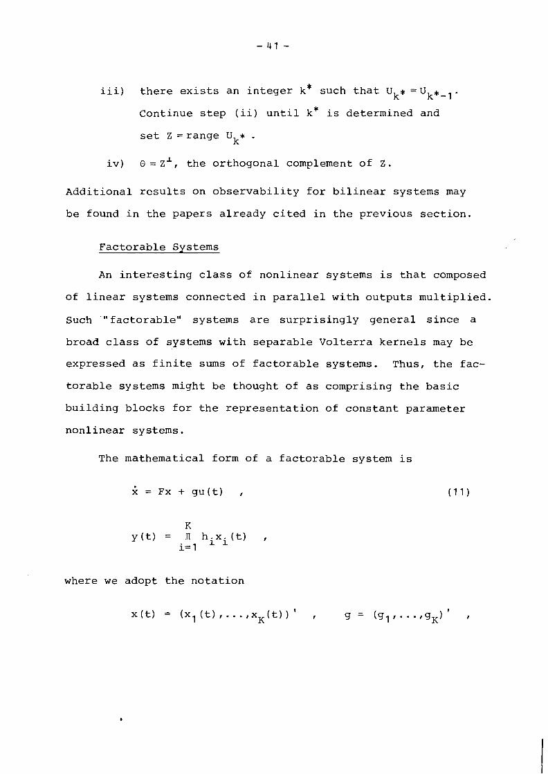
iii) there exists an integer k* such that U * =Uk*-l. k

Continue step (ii) until k* is determined and

set Z = range U * . k

I iv) 0 = Z , the orthogonal complement of Z .

Additional results on observability for bilinear systems may

be found in the papers already cited in the previous section.

Factorable Systems

An interesting class of nonlinear systems is that composed

of linear systems connected in parallel with outputs multiplied.

Such "factorable" systems are surprisingly general since a

broad class of systems with separable Volterra kernels may be .. . ~

expressed as finite sums of factorable systems. Thus, the fac-

torable systems might be thought of as comprising the basic

building blocks for the representation of constant parameter

nonlinear systems.

The mathematical form of a factorable system is

where we adopt the notation

x(t) = (xl (t) , . . . IXK(t)) I g = (g l f* . . fgK) l I

with xi being an ni-dimensional vector, and the elements hi, gi,

Fi being of corresponding sizes. Thus, the overall state vector

x(t) is of dimension n = nl +. . .+ n K '

Since the nonlinearity occurs only in the system output,

the usual reachability test from the linear theory shows that

the factorable system (11) is completely reachable if and only

if Wi(" and W.(A) have no poles in common for i # j , where 3

Wk(A) is the transfer matrix associated with the kth component

subsystem. Thus, we turn attention to study of the observability

properties of the system (1 1 ) .

It turns out to be convenient to investigate observability

for the system (11) by using the Kronecker product of the com-

ponent subsystems comprising (11). Letting

where 8 denotes the usual Kronecker product, it can be seen

8 that x (t) serves as a state vector for the linear system (with

u I 0 ) . We have

d 8 8 8 -x (t) = F x (t) , dt

with

F8 = F1 B I B . . .B I + In 8 F2 8 In @ . . . a I "2 "K 1 3 n K

8 Knowledge of the initial state x ( 0 ) enables us to compute (up

to certain ambiguities in sign) the state x(0). So, we say that

the system (11) is completely observable if its associated linear

system (12) is observable in the usual sense.

A convenient characterization of the observability of (12)

is possible if we define the vector A of distinct characteristic i

roots of the matrix F i.e., i '

<n. . The Kronecker sum of two such vectors where i=1,2, .-.,KI pi-

is given by

In terms of the Kronecker sum of the {Ail, we characterize

observability of (12) by the following result.

Theorem 21 [33] . The factorable system (1 1) is completely

observable if and only if the vector A l e A 2 @ ... @ A K has distinct

entries and at most one of the subsvstems has multi~le character-

istic values.

Polynomial Systems

Very few results exist on the observability question for

general continuous-time polynomial systems, i.e., systems of

the form

where P(-,-) and h(-) are polynomial functions of their arguments.

However, in the discrete-time case a considerable body of knowl-

edge has been reported in [341. For brevity, let us consider a

representative case, the so-called (polynomial) state-affine

system

where F ( - ) and G(-) are polynomial functions of u and H is a

constant matrix. A particular case is that of internally-

bilinear systems, when F and G are themselves linear functions

of u. The observability of the state-affine system (13) is

settled by the following test, which is a restatement of a

result taken from [341 .

Theorem 22 [ 3 4 ] . The input sequence w=ul,u2, ..., u,-I distinguishes all pairs of initial states for the state-affine

system (13) if and only if the matrix

0 (w) =

has rank n.

Thus, Theorem 21 shows that any input sequence w such that the

observability matrix O(w) is of full rank suffices to distinguish

initial states for the system (1 3) . For a more complete discussion of various observability

concepts for discrete-time polynomial systems and their inter-

relations, the work [ 3 4 ] should be consulted.

6. Realization Theory

The specification of the realization problem for linear

systems is simplified by the fact that it is easy to parametrize

the input, output and state spaces via a globally defined coordi-

nate system. This fact enables us to reduce the problem of

construction of a canonical model from input/output data to a

problem of linear algebra involving matrices. In the nonlinear

case no such global coordinate system exists, in general, and

it is necessary to take considerable care in defining what we

mean by the problem "data." We can no longer regard the input/

output data as being represented by an object as simple as an

infinite sequence of matrices or, equivalently, a matrix trans-

fer function. So, the first step in the construction of an

effective nonlinear realization procedure is to develop a

generalization of the transfer matrix suitable for describing

the input/output behavior of a reasonably broad class of non-

linear processes.

If we consider the nonlinear system (N)

then it is natural to attempt to represent the output of (N) in

terms of the input as a series expansion

Formally, the above Volterra series expansion is a generalization

of the linear variation of constant formula

y(t) = ~ e ~ ~ x 0 + jot He F(t-s)~u (s) ds .

Arguing by analogy with the linear case, the realization problem

for nonlinear systems may be expressed as: given the sequence

of Volterra kernels W= Iwo,wl,n2, ...I, find a canonical model

N = (f,h) whose input/output behavior generates $?K

Without further hypotheses on the analytic behavior of

f, h, together with a suitable definition of "canonical model,"

the realization problem as stated is much too ambitious and,

in general, unsolvable. F r , let us initially consider conditions

under which the Volterra series exists and is unique. Further,

we restrict attention to the class linear-analytic systems, i.e.,

f(x,u) =f(x) +u(t) g(x), where £ ( a ) , g(*) and h(.) are analytic

vector fields. The basic result for Volterra series expansions

is

Theorem 23 [35]. If f, g and h are analytic vector fields

and if ; = f(x) has a solution on [O,T] with x(0) = x,, then the

input/output behavior of (N) has a unique Volterra series repre-

sentation on [O,T] .

In the case of a bilinear system where f (x) = Fx, g(x) = Gx,

h(x) =x , u(*) = scalar control, the Volterra kernels can be

explicitly computed as

It can be shown [36] that for bilinear systems the Volterra

series converges globally for all locally bounded u.

The global convergence of the Volterra series for bilinear

processes suggests an approach to the construction of a Volterra

expansion in the general case. First, expand all functions in

their Taylor series, forming a sequence of bilinear approximations

of increasing accuracy. We then compute the Volterra series for

each bilinear approximation. However, the simple system

shows that, in general, no Volterra expansion exists which is

valid for all u such that 1 1 u 1 1 is sufficiently small. Further

details on the above bilinear approximation technique can be

found in [ I 81 .

By taking the Laplace transform of the Volterra kernels

{wilt it is possible to develop a nonlinear analogue of the

standard matrix transfer function of the linear theory. Such

an approach as carried out in [37], for example, provides an

alternate "frequency-domain" approach to the realization prob-

lem. We shall forego the details of such a procedure here due

to space considerations, and focus our attention solely upon

nonlinear systems whose input/output data is given in terms of

the infinite sequence of Volterra kernels (w.1. 1

Now let us turn to the definition of a canonical model for

a nonlinear process. As noted earlier, in the linear case we

say a model is canonical if it is both reachable (controllable)

and observable (constructible). Such a model is also minimal

in the sense that the state space ha9 smallest possible dimen-

sion (as a vector space) over all such realizations. In order

to preserve this minimality property, we make the following

Definition 14. A system ~-Ts--called locally weakly

minimal if it is locally weakly controllable and locally weakly

observable.

The relevance of Definition 14 to the realization problem

is seen from the following result.

Theorem 24 [ 1 7 ] . Let N,N be two nonlinear systems with

input sets R = h , and state manifolds M and M of dimensions m,m,

respectively. Suppose (N,x ) and (N,G ) realize the same input/ 0 0

output map. Then if N is -dcally weakly minimal, m < m . -

Thus, we see that two locally weakly minimal realizations of the

same input/output map must be of the same state dimension which

is minimal over all possible realizations.

Remark. Two locally weakly minimal realizations need not

be diffeomorphic, in contrast to the linear case. This is seen

from the two systems

N: x = u , y, = cos x , y2 = sin x ,

a

N: O = u , y, = cos 0 , y2 = sin@ ,

1 2 with n = 8 = ~ , M = R , M = S , the unit circle. ~ E R . x o = O , O = O . 0

Here N and N realize the same input/output map. Furthermore,

both systems are locally weakly controllable and observable.

The above result leaves open the question if two canonical

realizations are isomorphic, i.e., given two nonlinear systems

N and N, with state manifolds M and f i r

when does there exist a diffeomorphism I$ : M + M such that x=$(z),

The answer to this question is provided by the following re-

statement of a result of Sussman.

Theorem 25 [ 3 8 ] . Let there be given a mapping GxOrU

which to each input u(t) , O z t - < T, assigns a curve y(t) and

assume that there exists a finite-dimensional analytic complete

system

y = h ( x ) , X E M ,

which realizes the map Gxo,U . Then Gx can also be realized o t U

by a system which is weakly controllable and observable. Further-

more, any two such realizations are isomorphic.

Remark:

In all the results above, as well as those to follow, the

conditions of analyticity and completeness of the defining vector

fields is crucial. The reason is clear: analyticity forces a

certain type of "rigidity" upon the system, i.e, the global

behavior of the system is determined by its behavior in an

arbitrarily small open set. Completeness is also a natural

condition since without this property the system is not totally

specified, as it is then necessary to speak about the type of

behavior exhibited in the neighborhood of the vector field

singularity. Fortunately, analyticity and completeness are

properties possessed by any class of systems defined by sets

of algebraic equations, h - - - ~ n g a reasonable amount of homo-

geneity. For instance, linear systems, bilinear systems and

polynomial systems are all included in this class, together

with any other type of system which is both finite-dimensional

and "algebraic. "

Now let us turn to some realization results for specific

classes of nonlinear systems. For ease of notation, we consider

only single-input, single-output systems referring to the refer-

ences for the more general case.

Bilinear Systems

Given a sequence of Volterra kernels ( W ~ ~ I , ~ , the first

question is to determine conditions under which the sequence

may be realized by a bilinear system. For this we need the

concept of a factorizable sequence of kernels.

Definition 15. A sequence of kernels Iw.Ia is said to 1 i=2

be factorizable if there exist three matrix functions F(-),

G(-1, H( t lW) of sizes n x n , n x l , 1 xm, resp. such that

The set {F,GIH1 is called the factorization of {wi1 and the

number n is its dimension. A factorization lFOIG .H 1 of min- 0 0

imal dimension is called a minimal factorization.

We can now characterize those Volterra kernels which can

be realized by a bilinear system.

Theorem 26 [361. The sequence of Volterra kernels { ~ ~ l i = ~

is realizable by a bilinear system if and only if w, has a proper

rational Laplace transform and {w.lm 1 i=2 is factorizable by func-

tions F, G , H with proper rational Laplace transforms.

Let us assume that a given sequence of kernels {wi} is

bilinearly realizable. We then face the question of the con-

struction of a minimal realization and its properties. The main

result in this regard is

Theorem 27 [36]. For a sequence of bilinearly realizable

kernels {will the minimal realizations are such that

the state space dimension n is given by the dimension 0

of the linear system whose impulse response matrix is

ii) any two minimal realizations

are related by a linear transformation of their state spaces,

i.e., there exists an n x n matrix T such that 0-0

Theorem 27 provides the basic information needed in order to

actually construct the matrices A, B,C,N of a minimal realiza-

tion. Since W(s) is the impulse response of a linear system of

dimension n there must exist three matrices P, Q,R of sizes 0 ' no no x ("+I), (n+l) xno such that

By partitioning Q and R as

where R1 is 1 x n and Q1 is no x 1, we obtain 0

Ps G (s) = R2e Q1 1

0 Ps

F (s) = R2e Q2 . 0

We now define the matrices of our minimal realization as

Thus, the surprising conclusion is that the realization proce-

dure for bilinear systems can be carried out using essentially

the same techniques as those employed in the linear case once

the minimal factorization IF G ,H I has been found. 0' 0 0

Other approaches to the construction of bilinear realiza-

tions are discussed in [ 3 9 ] , while results for the discrete-

time case are given in [40]. The case of multilinear systems

is similar to the bilinear situation and is discussed in detail

in [ 4 1 1 .

Linear-Analytic Systems

The general question of when a given Volterra series

admits realization by a finite-dimensional linear-analytic system

{fIgrhI of the form

has no easily computable answer, although some difficult to test

conditions are given in [ 4 2 1 . On the other hand, if the Volterra

series is finite then the results are quite easy to check and

reasonably complete. For their statement, we make

Definition 16. A Volterra kernel w(t,sl, ..., sr) is called

separable if it can be expressed as a finite sum

It is called differentiably separable if each yi is differentiable

and is stationary if

The main theorem characterizing the realization of finite

Volterra series by a linear-analytic system is

Theorem 28 [42]. A finite Volterra series is realizable

by a (stationary) linear-analytic system if and only if each

term in the series is individually realizable by a (stationary)

linear-analytic system. Furthermore, this will be the case if

and only if the kernels are (stationary and differentiably)

separable.

The above result leaves open the question of actual com-

putation of the vector fields {f,g,h) defining the linear-

analytic realization of a finite Volterra series. However,

this problem is formally bypassed by the following result.

Theorem 29 [42]. A finite Volterra series has a (stationary)

linear-analytic realization if and only if it has a (stationary)

bilinear realization.

From Theorem 29 it is tempting to conclude that there is

no necessity to study linear-analytic systems when given a finite

Volterra series, since we can always realize the data with a

bilinear model. Unfortunately, the situation is not quite so

simple since the dimension of the canonical bilinear realization

will usually be somewhat greater than that of the corresponding

linear-analytic model. To illustrate this point, consider the

finite Volterra series

This series is realized by the three-dimensional bilinear model

= Fx + Gu + Nxu , where

y(t) = x(t) ,

However, the same set of kernels is also realized by the one-

dimensional linear-analytic system

& = sinx + u(t) ,

Polvnomial Svstems

If the system input/output map is of polynomial type, i.e.,

each term in the Volterra series is a polynomial function of its

arguments, then an elegant realization theory for such maps has

been developed by Sontag [ 2 7 ] in the discrete-time case. Since

presentation of the details would entail too large an excursion

into algebraic geometry, we loosely summarize the main results

referring to the references for a more complete account.

For simplicity, we restrict our account to bounded poly-

nomial input/output maps f, which means that there exists an

integer a such that the degree of each term in the Volterra

series for f is uniformly 'aunded by a. The main realization

result for bounded polynomial input/output maps is

Theorem 30 [ 2 7 ] . If a bounded input/output map is at all

realizable by a polynomial system, then it is realizable by an

observable state-affine system of the form

where F ( 0 ) and G ( 0 ) are polynomial matrices', H is a linear map

n and the system state space is R . An observable state-affine realization is termed span-

canonical if the subspace of reachable states is all of R".

Then it can be shown that a span-canonical realization of a

given bounded finitely realizable f always exists and any two

such realizations are related by a state coordinate change.

Furthermore, a realization is span-canonical if and only if

its dimension n is minimal among all state-affine realizations

of the same input/output map.

Somewhat less complete results are also reported in [ 2 7 ]

for unbounded polynomial input/output maps. The relationship

between the foregoing discrete-time results and the continuous-

time case is still far from clear, due mainly to the nonrevers-

ibility of difference (as opposed to differential) equations

and to the different algebraic properties of difference and

differential operations. To bridge this gap may turn out to

be a nontrivial task, as is seen by the recent result [ 4 3 ]

that a "finite" continuous-time map has its canonical state

space unconstrained, which is far from true in the discrete-

time setting.

Some additional work on polynomial systems taking a func-

tional-analytic, rather than algebraic, approach is reported

in [ 4 4 ] .

"Almostw-Linear Systems

By imposing special types of nonlinearities upon a standard

linear system, it is possible to employ techniques similar to

the usual linear methods for realization of input/output maps.

In this regard we note the "factorable" Volterra systems consid-

ered earlier, having the internal form

Here the nonlinearities enter only through the system output.

Utilizing tensor products, it can be shown [ 3 3 ] that the input/

output behavior of such a process can be described by a so-

called Volterra transfer function H(s,, ..., sK). Since a

factorable Volterra system consists of K linear subsystems

connected in parallel, with the outputs multiplied, the

realization problem reduces to determining the transfer func-

tions Hl (s) , . . . ,HK (s) of each subsystem from H (sl , . . . , sK) .

If the H=(S) are known. then standard linear theory provides the

overall system realization. Techniques for solving this problem

are reported in [ 331 .

In another direction. we could consider cascade combinations

of linear subsystems and static power nonlinearities as in [ 4 5 ] .

For inputs of the form

the output of such a system is

where m > 0 is an integer defining the degree of the static non-

linearity, i.e.. the block diagram of the system is

9 where ll P = m and H.(s) is a strictly proper rational func-

j=1 j 3

tion of degree 2 n. j =0.l, ...,q. In the work [ 4 5 ] an algorithm

is given for solution of the minimal realization problem for such

a system.

7. Conclusions and Future Research

The foregoing results leave little doubt that substantial

progress has been made in nonlinear system theory over the past

decade. As noted in the introduction, we have focused only

upon problems of reachability, observability and realization,

omitting the more well-known areas of stability and optimal

control. Advances in these areas have also been impressive as

can be seen from the works [46-471. Thus, the inescapable

conclusion is that nonlinear system theory is alive and well

and it is to be expected that progress on outstanding issues

will be rapid in the years to come.

By way of closing remarks, let us now engage in a bit of

crystal ball-gazing and sketch some problem areas which seem

to be most important for future research in nonlinear systems.

1) Computational Methods -the effective employment of

any of the results given here relies upon efficient computational

algorithms. For those procedures which mimic the linear case

(e.g., bilinear realization), good methods already exist for

computing the necessary quantities. However, much remains to

be done to develop comparable methods for, say, computing the

reachable set for a nonlinear process or determining the Volterra

series of a given input/output map from measured data;

2) Stochastic Effects - a cornerstone of linear system

theory is the Kalman filter and its associated apparatus for

determining the "best" estimate of system parameters in the

presence of noise. This is a special case of the more general

stochastic realization problem, in which the input/output data

i t s e l f i s c o r r u p t e d by n o i s e and " b e s t " e s t i m a t e s o f t h e system

model must be made. Again i n t h e l i n e a r c a s e r e s u l t s a r e a v a i l -

a b l e [ 48 ] . However, a lmos t no th ing has been accompl ished a long

t h e s e l i n e s f o r n o n l i n e a r ::ocesses. I t seems l i k e l y , though,

t h a t w i t h t h e i n c r e a s e d unders tand ing now a v a i l a b l e good p rog ress

can be made. W e shou ld n o t e t h e works [49-501 a s promis ing

i n i t i a l f o r a y s i n t h i s a r e a ;

3 ) on-~nalytic Systems - a lmos t a l l i n t e r e s t i n g r e s u l t s

f o r n o n l i n e a r sys tems are f o r p rocesses whose d e f i n i n g v e c t o r

f i e l d s a r e a n a l y t i c . A s po in ted o u t e a r l i e r , t h e r e i s good

reason f o r t h i s s i n c e t h e l o c a l behav io r o f a n a l y t i c sys tems

e n t i r e l y de te rm ines t h e g l o b a l behav io r . However, t h e r e a r e

i n t e r e s t i n g and impor tan t p rocesses which do n o t f a l l i n t o

t h i s ca tego ry (e .g . , sys tems w i t h t h r e s h o l d e f f e c t s , p rocesses

w i t h phase t r a n s i t i o n s , and s o o n ) . A c o n c e r t e d a t t e m p t a t

r e l a x a t i o n o f t h e a n a l y t i c i t y assumpt ions can b e expec ted t o

y i e l d s u b s t a n t i a l d i v i dends i n f u r t h e r i n g o u r a b i l i t y t o t a c k l e

a v a r i e t y of problems i n t h e s o c i a l and b i o l o g i c a l s c i e n c e s ;

4 ) I n f i n i t e -D imens iona l P rocesses - i n g e n e r a l , systems

whose unde r l y i ng dynamics a r e governed by p a r t i a l d i f f e r e n t i a l

equa t i ons o r p r o c e s s e s i nvo l v i ng t ime- lag e f f e c t s canno t be

modeled by a f i n i t e set o f o r d i n a r y d i f f e r e n t i a l o r d i f f e r e n c e

equa t i ons . Even i n t h e l i n e a r c a s e such p r o c e s s e s l e a d t o

tho rny a n a l y t i c a l q u e s t i o n s which a r e , as y e t , f a r from be ing

w e l l under c o n t r o l . So, it i s perhaps w i l d l y o p t i m i s t i c t o

t h i n k t h a t s u b s t a n t i a l advances can be made i n t h i s d i r e c t i o n

f o r n o n l i n e a r p r o c e s s e s . None the less , w e have seen t h a t many

of the results and techniques of the linear theory can be

extended to classes o f nonlinear systems with modest additional

effort. So, it seems reasonable to attempt an investigation

of those nonlinear problems which are the counterparts of the

corresponding infinite-dimensional linear processes.

References

[I I Mayne, D., and R. Brockett, eds., Geometric Methods in

System Theory, Reidel, Dordrecht, 1973.

[2] Martin, C., and R. Hermann, eds., The 1976 Ames Research

Center (NASA) Conference on Geometric Control Theory,

Math Sci Press, Brookline, Mass., 1977.

[31 Byrnes, C., and N. Hurt, On the Moduli of Linear Dynamical

Systems, Advances in Mathematics, - 4 (1979), 83-122.

[4] Hermann, R., Linear System Theory and Introductory Algebraic

Geometry, Interdisciplinary Mathematics, Vol. 8, Math

Sci Press, Brookline, Mass., 1974.

[5] Fuhrmann, P., Algebraic System Theory: An Analyst's Point

of View, J. Franklin Institute, 301 (1976), 521-540.

[6] Kalman, R., P. Falb, and M. Arbib, Topics in Mathematical

System Theory, McGraw-Hill, New York, 1969.

[71 Casti, J., Dynamical Systems and their Applications: Linear

Theory, Academic Press, New York, 1977.

[81 Brockett, R., Finite-~imensional Linear Systems, John Wiley,

New York, 1970.

[9] Kalman, R.E., On Partial Realizations of a Linear Input/

Output Map, in N. de Claris and R. Kalman, eds.,

Systems and Networks, Holt, New York, 1968.

[lo] Kalman, R.E., On Partial Realizations, Transfer Functions

and Canonical Forms, Acta Polytechnica Scandinavica,

31 (1979), 9-32. -

[Ill Bryson, A., and Y.C. Ho, Applied Optimal Control, Blaisdell,

Waltham, Mass., 1969.

[I21 Aggarwal, J., and M. Vidyasagar, eds., Nonlinear Systems:

Stability Analysis, Dowden, Hutchinson and Ross,

Stroudsburg, Penn., 1977.

1131 Peixoto, M., ed., Dynamical Systems, Academic Press, New

York, 1973.

[I41 Lee, E., and L. Markus, Foundations of Optimal Control,

John Wiley, New York, 1967.

[I51 Brockett, R., On the Reachable Set for Bilinear Systems,

in R. Mohler and A. Ruberti, eds., Proc. 1974

Conference on Bilinear Systems, Springer, New York,

1975.

[16] Kalman, R.E., Pattern Recognition Problems of Multilinear

Machines, in Proc. IFAC Symposium on Technical and

Biological Problems of Control, Yerevan, Armenia,

USSR, 1968.

[I71 Hermann, R., and A. Krener, Nonlinear Controllability and

Observability, IEEE Transactions on Automatic Control,

AC-22 (1977), 728-740.

[I81 Brockett, R., Nonlinear Systems and Differential Geometry,

Proc. IEEE, - 64 (1976), 61-72.

[I91 Hermes, H., On Local and Global Controllability, SIAM

Journal of Control, - 12 (1974), 252-261.

[20] Hirschorn, R., Global Controllability of Nonlinear Systems,

SIAM Journal of Control, 14(1976), 700-711.

[21] Haynes, G.W., and H. Hermes, Nonlinear Controllability

via Lie Theory, SIAM Journal of Control, - 8 (1970),

450-460.

[22] Sussman, H., and V. ,,rdjevic, Controllability of Nonlinear

Systems, Journal of Differential Equations, - 12 (1972),

95-1 16.

[23] Mohler, R., Bilinear Control Processes, Academic Press,

New York, 1973.

[24] Sussman, H., and V. Jurdjevic, Control Systems on Lie

Groups, Journal of Differential Equations, - 12 (1972).

[25] Imbert, N., M. Clique, and A.-J. Fossard, Un ~r i tgre de

~ouvernabilitg des SystGmes ~ilin&aires, RAIRO,

J-3 (1979), 55-64.

1261 Lukes, D.L., On the Global Controllability of Nonlinear

Systems, in L. Weiss, ed., Ordinary Differential

Equations, Academic Press, New York, 1971.

[27] Sontag, E., Polynomial Response Maps, Springer Lecture

Notes in Control, Vol. 13, Berlin, 1979.

[281 Griffith, E., and K.S.P. Kumar, On the Observability of

Nonlinear Systems - I , Journal of Mathematical Analysis

and Applications, - 35 (1971), 135-147.

1291 KOU, S.R., D. Elliott, and T.J. Tarn, Observability of

Nonlinear Systems, Information and Control, - 22 (1973),

89-99.

[30] Kostynkovskii, Y., Observability of Nonlinear Controlled

Systems, Automation and Remote Control, - 9 (1968),

1384-1 396.

[31] Brockett, R., On the Algebraic Structure of Bilinear

Systems, in R. Mohler and A. Ruberti, eds., Theory

and Application of Variable Structure Systems,

Academic Press, New York, 1972.

[321 Isidori, A., and A. Ruberti, Realization Theory of

Bilinear Systems, in [ 1 ] .

[33] Harper, T., and W. Rugh, Structural Features of Factorable

Volterra Systems, IEEE Transactions on Automatic

Control, AC-21 (1976), 822-832.

[34] Sontag, E., On the Observability of Polynomial Systems, I:

Finite-Time Problems, SIAM Journal of Control, - 17

(1979), 139-151.

[351 Lesiak, C., and A. Krener, The Existence and Uniqueness of

Volterra Series for Nonlinear Systems, IEEE Trans-

actions on Automatic Control, AC-23 (1978), 1090-1095.

[36] dlAlessandro, P., A. Isidori, and A. Ruberti, Realization

and Structure Theory of Bilinear Systems, SIAM

Journal of Control, 12 (1974), 517-535. -

[37] Mitzel, G., S. Clancy, and W. Rugh, On Transfer Function

Representation for Homogeneous onl linear Systems,

IEEE ~ransactions on Automatic Control, AC-24 (1979),

242-249.

[381 Sussman, H., Minimal Realizations of Nonlinear Systems,

in [I].

[39] Isidori, A,, Direct Construction of Minimal Bilinear

Realizations from Nonlinear Input/Output Maps, IEEE

Transactions on Automatic Control, AC-18 (1973)

[401 Fornasini, E., and G. Marchesini, Algebraic Realization

Theory of Bilinear Discrete-Time Input/Output Maps,

J. Franklin Institute, 301 (1976), 143-159.

[411 Marchesini, G., and b. Picci, Some Results on the Abstract

Realization Theory of Multilinear Systems, in R. Mohler

and A. Ruberti, eds., Theory and Application of Vari-

able Structure Systems, Academic Press, New York, 1972.

[421 Brockett, R., Volterra Series and Geometric Control Theory,

[43] Crouch, P., Finite Volterra Series, doctoral dissertation,

Harvard University, 1977.

[44] Porter, W.A., An Overview of Polynomic System Theory,

Proc. IEEE, 64 (1976), 18-23. -

[45] Smith, W., and W. Rugh, On the Structure of a Class of

Nonlinear Systems, IEEE Transactions on Automatic

Control, AC-19 (1974), 701-706.

[461 Gurel, O., and 0. Rassler, eds., Bifurcation Theory and

Applications in Scientific Disciplines, NY Academy

of Sciences, Vol. 316, 1979.

[471 Brunovsky, P., On the Structure of Optimal Feedback Systems,

Proc. International Congress of Mathematicians,

Helsinki, 1978.

[48] Picci, G., Stochastic Realization of Gaussian Processes,

Proc. IEEE, 64 (1976), 112-122. -

[49] Willsky, A., and S. Marcus, Analysis of Bilinear Noise

Models in Circuits and Devices, J. Franklin Institute,

[ 5 0 ] Marcus, S., Modeling and Analysis of Linear Systems with

Multiplicative Poisson White Noise, in [ 2 ] .