Embed Size (px)
Citation preview
Recommendations onBase Station Antenna Standardsv11.1

Address:
ngmn e. V.
Großer Hasenpfad 30 • 60598 Frankfurt • Germany
Phone +49 69/9 07 49 98-0 • Fax +49 69/9 07 49 98-41
Recommendation on Base Station
Antenna Standards by NGMN Alliance
Version: 11.1
Date: 06-03-2019
Document Type: Final Deliverable (approved)
Confidentiality Class: P - Public
© 2019 Next Generation Mobile Networks e.V. All rights reserved. No part of this document may be reproduced or transmitted in any form or by any means without prior written permission from NGMN e.V.
The information contained in this document represents the current view held by NGMN e.V. on the issues discussed as of the date of publication. This document is provided “as is” with no warranties whatsoever including any warranty of merchantability, non-infringement, or fitness for any particular purpose. All liability (including liability for infringement of any property rights) relating to the use of information in this document is disclaimed. No license, express or implied, to any intellectual property rights are granted herein. This document is distributed for informational purposes only and is subject to change without notice. Readers should not design products based on this document.
t
Page 2 N-P-BASTA Whitepaper
Version 11.1 6th March 2019
Project: N-P-BASTA
Submitter: André F.A. Fournier (Amphenol Antenna Solutions)
Editors: André F.A. Fournier (Amphenol Antenna Solutions)
Contributors: Amphenol Antenna Solutions
Commscope
CellMax
Deutsche Telekom
Huawei
Kathrein
NEC
RFS
Rosenberger
Telecom Italia
Telefonica
Telekom Austria
Approved by / Date: NGMN Board, February 15, 2019
t
Page 3 N-P-BASTA Whitepaper
Version 11.1 6th March 2019
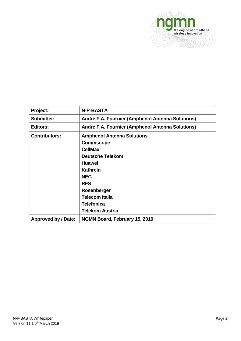
Abstract
This whitepaper addresses the performance criteria of base station antennas, by making recommendations
on standards for electrical and mechanical parameters, by providing guidance on measurement and
calculation practices in performance validation and production, and by recommending methods for
electronic data exchange. It also addresses recommendations on applying existing environmental and
reliability standards to BSAs.
NGMN Project-BASTA
Measurement
procedures
Parameter definitions
&
Calculation methods
Datasheet creation
&
Delivery
t
Page 4 N-P-BASTA Whitepaper
Version 11.1 6th March 2019
Changes from version 10.0
Added several definitions throughout the document.
Notes are enumerated using section number and sequential number example
Parameter definitions and their specification definitions corrected.
Notes added in the whole document to better specify definitions, scopes, etc.
Corrected some errors in formulas
Format of the whole whitepaper corrected.
Section 1.1 added the section 1.1 titled INTERPRETATION.
Section 1.2 References added the IEC 62037-6 for PIM reference
Created Section 2.1 and moved the ABBREVIATION from an APPENDIX
Section 2.2 add a reference table 2.2-1 for antenna terms
Section 2.5, 2.7 2.11 and 4.5 updated the text and figures to align with 3GPP standards
Some general wording improvement throughout the document
Section 3.2.1 removed the reference to the SECTOR & based on the feedback added the word
SECTOR in parenthesis
Section 3.2.5 rephrase the parameter definition
Section 3.2.13 changed the section title and content from Cross-Polar to Intra-Cluster
Section 3.2.16 in the Specification Definition replaced the word “MAXIMUM’ with a better definition
Section 3.2.17 in the Specification Definition replaced the word “MAXIMUM’ with a better definition
Section 3.2.19 improved the wording to the Parameter definition
Section 3.2.20 improved the wording to the Parameter definition
Section 3.2.21 changed the section title and content from Interband to Inter-Cluster
Removed section 3.3.1 because topic already covered in other sections
Section 3.3.4 titled changed from Cross-Polar Discrimination at Mechanical Boresight to Cross-Polar
Discrimination over 3 dB Azimuth Beamwidth
Section 3.3.12 changed the title from Maximum Upper Sidelobe Level to Maximum Upper Sidelobe
Suppression and updated the section to reflect the new title
Section 3.3.13 corrected the AIR formula to align with the description
Section 3.3.14 Azimuth Nominal Beamwidth was moved to create Section 3.2.22 because the
parameter is required for multi-beam type II antennas. The moving of this section caused an
numbering adjustment in the following section
Updated Section 4.2 General Guidance point related to 3dB delta between values
Section 5.1 Antenna Dimensions improved the wording.
Section 5.7 Connector Quantity added a drawing of an antenna bottom plate
Added the section 5.9 titled Windload – Calculation Guideline
Note 5.9.0-1 Removed part of the note in reference to the Maximum Wind Load specification
requirements.
Added subsection 5.9.1 titled Windload – Frontal
Added subsection 5.9.2 titled Windload – Lateral
Section 7.3.11 added the level of impact UV/Weather test and change the title to Solar/Weather
Section 7.3.11 corrected the IEC Ex standard IEC Ex 60068-2-18 to IEC Ex 60068-2-5
Section 7.3.13 added the antenna weight of <50kg and >50kg for test consideration
Section 9.1.3 removed the note 9.1.0.1 it was misleading
Section 9.3.2 Gain by Directivity/Loss Method corrected the formula and improved the information
Section 9.5 updated the PIM to include the mention of the IEC Ex 62037-6 as a reference
Appendix A Example of Antenna Datasheet updated the datasheet to align the changes in the
document and removed the reference to NOMINAL HORIZONTAL HPBW parameter

t
Page 5 N-P-BASTA Whitepaper
Version 11.1 6th March 2019
Appendix B Example of RET Datasheet updated the datasheet to align the changes in the
document
Appendix C Logical Bloc Structure (Antenna+RET) updated the datasheet to align the changes
in the document
Appendix D Example of Antenna XML file updated the datasheet to align the changes in the
document
Appendix E Example of RET XML file updated the datasheet to align the changes in the document
Added an appendix F titled test config. & windload extrapolation. Provided examples
Added an appendix G describing the changes between Version 9.6 and Version 10

t
Page 6 N-P-BASTA Whitepaper
Version 11.1 6th March 2019
Table of Contents Recommendation on Base Station ................................................................................................................................... 1 Antenna Standards ............................................................................................................................................................ 1
Changes from version 10.0 ........................................................................................................................................ 3 1 Introduction and Purpose of Document .................................................................................................................. 12
1.1 Interpretation .................................................................................................................................................. 12 1.2 References ..................................................................................................................................................... 13
2 Abbreviations and Antenna Terms Definitions ....................................................................................................... 14 2.1 Abbreviations .................................................................................................................................................. 14 2.2 Antenna terms ................................................................................................................................................ 15 2.3 Array and Cluster ........................................................................................................................................... 16 2.4 Radiation Intensity .......................................................................................................................................... 16 2.5 Antenna Reference Coordinate System ....................................................................................................... 16 2.6 Far-Field Radiation Pattern ........................................................................................................................... 17 2.7 Far-Field Radiation Pattern Cut .................................................................................................................... 17 2.8 Total Power Radiation Pattern Cut ............................................................................................................... 18 2.9 Beams and Antenna Classes ........................................................................................................................ 18 2.10 Half-Power Beamwidth .................................................................................................................................. 20 2.11 Electrical Downtilt Angle ................................................................................................................................ 20
3 Parameter and Specifications .................................................................................................................................. 21 3.1 Format ............................................................................................................................................................. 21 3.2 Required RF Parameters .............................................................................................................................. 23
3.2.1 Antenna Reference, Nominal Sector and Nominal Directions ............................................................... 23 3.2.2 Frequency Range and Frequency Sub-Range ....................................................................................... 24 3.2.3 Polarization ................................................................................................................................................ 24 3.2.4 Gain ............................................................................................................................................................ 25 3.2.5 Gain Ripple ................................................................................................................................................ 26 3.2.6 Azimuth Beamwidth................................................................................................................................... 27 3.2.7 Elevation Beamwidth ................................................................................................................................. 28 3.2.8 Electrical Downtilt Range .......................................................................................................................... 29 3.2.9 Elevation Downtilt Deviation ..................................................................................................................... 29 3.2.10 Impedance ............................................................................................................................................. 30 3.2.11 Voltage Standing Wave Ratio .............................................................................................................. 31 3.2.12 Return Loss ........................................................................................................................................... 32 3.2.13 Intra-Cluster Isolation ............................................................................................................................ 33 3.2.14 Passive Intermodulation ....................................................................................................................... 35 3.2.15 Front-to-Back Ratio, Total Power, ± 30° .............................................................................................. 36 3.2.16 First Upper Sidelobe Suppression ....................................................................................................... 37 3.2.17 Upper Sidelobe Suppression, Peak to 20° .......................................................................................... 38 3.2.18 Cross-Polar Discrimination over Sector .............................................................................................. 39 3.2.19 Maximum Effective Power per Port ..................................................................................................... 40 3.2.20 Maximum Effective Power Whole Antenna ......................................................................................... 41 3.2.21 Inter-Cluster Isolation ............................................................................................................................ 41 3.2.22 Azimuth Nominal Beam Directions ...................................................................................................... 43
3.3 Optional RF Parameters ................................................................................................................................ 44 3.3.1 Azimuth Beam Squint ................................................................................................................................ 44 3.3.2 Null Fill ........................................................................................................................................................ 45 3.3.3 Cross-Polar Discrimination at Mechanical boresight .............................................................................. 46 3.3.4 Cross-Polar Discrimination over 3 dB Azimuth Beamwidth .................................................................... 48 3.3.5 Cross-Polar Discrimination over 10 dB Azimuth Beamwidth ................................................................. 49 3.3.6 Cross Polar Discrimination over 3 dB Elevation Beamwidth .................................................................. 50

t
Page 7 N-P-BASTA Whitepaper
Version 11.1 6th March 2019
3.3.7 Cross Polar Discrimination over 10 dB Elevation Beamwidth ................................................................ 51 3.3.8 Azimuth Beam Port-to-Port Tracking ....................................................................................................... 51 3.3.9 Azimuth Beam H/V Tracking .................................................................................................................... 52 3.3.10 Azimuth Beam Roll-Off ......................................................................................................................... 54 3.3.11 Upper Sidelobe Suppression, Horizon to 20° ..................................................................................... 55 3.3.12 Maximum Upper Sidelobe Suppression .............................................................................................. 56 3.3.13 Azimuth Interference Ratio ................................................................................................................... 57 3.3.14 Azimuth Beam Pan Angles .................................................................................................................. 58 3.3.15 Azimuth Beamwidth Fan ...................................................................................................................... 59 3.3.16 Maximum Effective Power of Cluster................................................................................................... 61
4 Validation and Specification of RF Parameters ...................................................................................................... 62 4.1 Industry Practice for Base Station Antennas ................................................................................................ 62 4.2 General Guidance .......................................................................................................................................... 62 4.3 Absolute RF Parameters ............................................................................................................................... 63 4.4 Distribution-based RF Parameters ............................................................................................................... 64
4.4.1 General methodology ................................................................................................................................ 64 4.4.2 Double-Sided Specifications ..................................................................................................................... 65 4.4.3 Double-Sided Specification Example–Azimuth HPBW Validation ......................................................... 66 4.4.4 Single-sided Specifications ....................................................................................................................... 69 4.4.5 Single-sided Specification Example – Azimuth Beam Port-to-Port Tracking Validation ....................... 70 4.4.6 Single-sided Specification Example – Upper Sidelobe Suppression, Peak to 20° Validation ............. 73
4.5 Sidelobe Suppression Calculation and Validation ....................................................................................... 76 4.5.1 First Sidelobe Suppression ....................................................................................................................... 77 4.5.2 Null fill ......................................................................................................................................................... 78 4.5.3 Upper Sidelobe Suppression, Peak to 20° / Horizon to 20° ................................................................... 78
4.6 Gain Validation ............................................................................................................................................... 79 4.6.1 Gain Validation for a Single Tilt Value ...................................................................................................... 79 4.6.2 Gain Over All Tilts Validation .................................................................................................................... 82
4.7 Validation of Elevation Downtilt Deviation .................................................................................................... 85 4.8 Guidance on Specifications Provided in Radio Planning Files ................................................................... 88
5 Mechanical Parameters and Specifications ............................................................................................................ 88 5.1 Antenna Dimensions ...................................................................................................................................... 88 5.2 Packing Size ................................................................................................................................................... 89 5.3 Net Weight ...................................................................................................................................................... 90 5.4 Shipping Weight ............................................................................................................................................. 90 5.5 Connector Type .............................................................................................................................................. 91 5.6 Connector Quantity ........................................................................................................................................ 91 5.7 Connector Position ......................................................................................................................................... 92 5.8 Survival Wind Speed ..................................................................................................................................... 93 5.9 Windload – Calculation Guideline ................................................................................................................. 93
5.9.2 Windload – Frontal .................................................................................................................................... 94 5.9.3 Windload – Lateral ..................................................................................................................................... 95
5.10 Radome Material ............................................................................................................................................ 96 5.11 Radome Color ................................................................................................................................................ 96 5.12 Product Environmental Compliance ............................................................................................................. 96 5.13 Mechanical Distance between Antenna Mounting Points ........................................................................... 97 5.14 Mechanical Distance between Pole Mounting Points.................................................................................. 98 5.15 Lightning Protection ....................................................................................................................................... 99
6 Remote Electrical Tilt System .................................................................................................................................. 99 6.1 Actuator Size ................................................................................................................................................ 100 6.2 Working Temperature Range ...................................................................................................................... 103 6.3 Power Consumption .................................................................................................................................... 103

t
Page 8 N-P-BASTA Whitepaper
Version 11.1 6th March 2019
6.4 Loss of Position on Power Failure .............................................................................................................. 104 6.5 Compatible Standards ................................................................................................................................. 104 6.6 Compatible Proprietary Protocols ............................................................................................................... 105 6.7 Configuration Management ......................................................................................................................... 105 6.8 Antenna Configuration File Availability ....................................................................................................... 106 6.9 Antenna Configuration File Upgradability ................................................................................................... 106 6.10 Software Upgradability ................................................................................................................................. 107 6.11 Replaceability in Field .................................................................................................................................. 107 6.12 Visual Indicator Available on Tilt Change ................................................................................................... 108 6.13 Daisy Chain Available .................................................................................................................................. 109 6.14 Smart Bias-T Available ............................................................................................................................... 109
7 Environmental Standards....................................................................................................................................... 110 7.1 Base Station Antenna Environmental Criteria ............................................................................................ 110 7.2 Environmental Test Approach ..................................................................................................................... 111 7.3 Environmental Test Methods ...................................................................................................................... 111
7.3.1 Packaged Storage ................................................................................................................................... 112 7.3.2 Cold Temperature Survival ..................................................................................................................... 112 7.3.3 Hot Temperature Survival ....................................................................................................................... 112 7.3.4 Temperature Cycling ............................................................................................................................... 112 7.3.5 Vibration – Sinusoidal .............................................................................................................................. 112 7.3.6 Humidity Exposure .................................................................................................................................. 113 7.3.7 Rain .......................................................................................................................................................... 113 7.3.8 Water Ingress........................................................................................................................................... 113 7.3.9 Dust and Sand Ingress ............................................................................................................................ 113 7.3.10 Survival Wind Speed .......................................................................................................................... 113 7.3.11 Solar/Weather Exposure .................................................................................................................... 114 7.3.12 Corrosion Resistance ......................................................................................................................... 114 7.3.13 Shock & Bump .................................................................................................................................... 115 7.3.14 Free Fall (Packaged Product) ............................................................................................................ 115 7.3.15 Broadband Random Vibration ........................................................................................................... 116 7.3.16 Steady State Humidity ........................................................................................................................ 116
8 Reliability Standards ............................................................................................................................................... 116 9 Additional Topics .................................................................................................................................................... 117
9.1 Recommended Sub-bands and Associated Frequency List..................................................................... 117 9.1.1 Frequency Ranges Choice Method ....................................................................................................... 119 9.1.2 Frequency Samples Choice Method ...................................................................................................... 126 9.1.3 Compatibility with old whitepaper versions and use of non-BASTA frequencies ................................ 131
9.2 Guidance on Pattern and Gain Measurements ......................................................................................... 131 9.2.1 Mechanical Alignment of Test System ................................................................................................... 131 9.2.2 Phase Center Check ............................................................................................................................... 131 9.2.3 Antenna Pattern Testing ......................................................................................................................... 131 9.2.4 Pattern Accuracy Estimation ................................................................................................................... 132
9.3 Gain Measurement ...................................................................................................................................... 132 9.3.1 Gain by Substitution Method ................................................................................................................... 132 9.3.2 Gain by Directivity/Loss Method ............................................................................................................. 132
9.4 On the Accuracy of Gain Measurements ................................................................................................... 135 9.4.1 Antenna Mismatch between Reference Antenna and AUT ................................................................. 135 9.4.2 Size Difference between Reference Antenna and AUT ....................................................................... 135 9.4.3 Temperature and Humidity Drift in Instruments ..................................................................................... 135 9.4.4 Polarization .............................................................................................................................................. 135 9.4.5 Direct Gain Comparison Between Two Antennas ................................................................................ 136 9.4.6 Reference Antennas ............................................................................................................................... 136

t
Page 9 N-P-BASTA Whitepaper
Version 11.1 6th March 2019
9.5 Guidance on Production Electrical Testing ................................................................................................ 136 9.6 Recommend Vendor’s Reference Polarization Labelling Convention ..................................................... 137
10 Format for the Electronic Transfer of Specification Data ............................................................................... 138 10.1 XML use for BSA specifications .................................................................................................................. 139
10.1.1 Filename .............................................................................................................................................. 141 10.1.2 Preamble ............................................................................................................................................. 142 10.1.3 Antenna ............................................................................................................................................... 143 10.1.4 Electrical Specifications ...................................................................................................................... 143 10.1.5 Cluster.................................................................................................................................................. 143 10.1.6 Sub-Band............................................................................................................................................. 145
11 Note: Tolerances are intended as plus or minus (±). ..................................................................................... 146 11.1.1 Mechanical and Environmental Specifications ................................................................................. 146 11.1.2 Miscellaneous data ............................................................................................................................. 147
11.2 XML use for RET specifications .................................................................................................................. 147 APPENDIX A – EXAMPLE OF ANTENNA DATASHEET .......................................................................................... 149 APPENDIX B – EXAMPLE OF RET DATASHEET ..................................................................................................... 150 APPENDIX C – LOGICAL BLOCK STRUCTURE (ANTENNA+RET) ....................................................................... 151 APPENDIX D – EXAMPLE OF ANTENNA XML FILE ................................................................................................ 152 APPENDIX E – EXAMPLE OF RET XML FILE ........................................................................................................... 156 APPENDIX F – TEST CONFIG. & WINDLOAD EXTRAPOLATION ......................................................................... 157 APPENDIX G – CHANGES FROM VERSION 9.6 TO VERSION 10.0 ..................................................................... 163
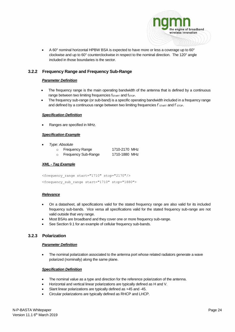
List of Figures Figure 2.3-1—Possible difference between array and clusters..................................................................................... 16 Figure 2.5-1—Antenna Reference Coordinate System. ................................................................................................ 17 Figure 2.7-1—Cuts over the radiation sphere. ............................................................................................................... 18 Figure 2.9-1—Example of a dual-beam antenna. .......................................................................................................... 19 Figure 2.9-2—Azimuth pattern of a multi-beam antenna type II. .................................................................................. 20 Figure 2.11-1—Electrical downtilt angle. ........................................................................................................................ 21 Figure 3.2-1—Calculation of azimuth beamwidth. ......................................................................................................... 27 Figure 3.2-2—Example of VSWR measurement of an antenna port. .......................................................................... 32 Figure 3.2-3—Example of a return loss measurement on a single antenna port. ....................................................... 33 Figure 3.2-4—Intra-Cluster isolation example: single cluster antenna. ........................................................................ 33 Figure 3.2-5—Intra-Cluster isolation example: dual cluster antenna. ........................................................................... 34 Figure 3.2-6—Example of a intra-cluster isolation measurement between two antenna ports. ................................. 35 Figure 3.2-7—Angular region for front-to-back, total power ± 30° of a 0° nominal direction antenna. ....................... 36 Figure 3.2-8—First upper sidelobe suppression. ........................................................................................................... 37 Figure 3.2-9—Upper sidelobe suppression, peak to 20º. .............................................................................................. 38 Figure 3.2-10—Cross-polar discrimination over sector of a 0° mechanical boresight, 60° nominal horizontal HPBW
antenna. ............................................................................................................................................................................ 39 Figure 3.2-11—Inter-Cluster isolation examples. In this example, the inter-cluster isolation is the worst case of S41,
S31, S42 and S32. ........................................................................................................................................................... 42 Figure 3.2-12—Inter-cluster isolation vs. frequency on a single pair of ports. ............................................................. 43 Figure 3.3-1—Illustration of beam squint calculation for a given frequency, tilt and port. ........................................... 44 Figure 3.3-2—Identification of the lower first null. .......................................................................................................... 45 Figure 3.3-3—Cross-polar discrimination at mechanical boresight. ............................................................................. 47 Figure 3.3-4—Cross pol discrimination over 3 dB azimuth beamwidth. ....................................................................... 48 Figure 3.3-5—Cross pol discrimination over 10 dB azimuth beamwidth. ..................................................................... 49 Figure 3.3-6—Azimuth beam port-to-port tracking. ........................................................................................................ 52 Figure 3.3-7—Azimuth beam H/V tracking. .................................................................................................................... 53 Figure 3.3-8—Azimuth beam roll-off. .............................................................................................................................. 54

t
Page 10 N-P-BASTA Whitepaper
Version 11.1 6th March 2019
Figure 3.3-9—Upper sidelobe suppression, horizon to 20º. .......................................................................................... 55 Figure 3.3-10—Maximum Upper Sidelobe Suppression. .............................................................................................. 56 Figure 3.3-11—Some patterns of an azimuth beam steering antenna (pan angles: -30°; 0°; +30°). ......................... 59 Figure 3.3-12— Patterns of a variable azimuth beamwidth BSA (35°/65°/105° pattern overlays). ............................ 60 Figure 4.4-1—Double-sided specification for a normal distribution. ............................................................................. 65 Figure 4.4-2—Algorithm to find "mean - tolerance" and "mean + tolerance" ............................................................... 66 Figure 4.4-3—Azimuth beam-peak patterns plots - 1710-1880 MHz, all ports, and all tilts. ....................................... 66 Figure 4.4-4—Azimuth HPBW for each tilt and port as a function of the frequency. ................................................... 68 Figure 4.4-5—Histogram of azimuth HPBW values. ..................................................................................................... 68 Figure 4.4-6—Single-sided specification (maximum). ................................................................................................... 69 Figure 4.4-7—Single-sided specification (minimum). .................................................................................................... 70 Figure 4.4-8—Algorithm to find "maximum" and "minimum". ........................................................................................ 70 Figure 4.4-9—Polarizations pattern level difference of a 90° sector antenna for one frequency and a single downtilt
degree. .............................................................................................................................................................................. 71 Figure 4.4-10—Azimuth beam port-to-port tracking for each tilt and port as a function of the frequency. ................. 72 Figure 4.4-11—Histogram azimuth beam port-to-port tracking. .................................................................................... 73 Figure 4.4-12—Worst sidelobe peak 20° above the main beam peak for one frequency, a single port and a single
downtilt degree. ................................................................................................................................................................ 74 Figure 4.4-13—Upper sidelobe suppression, peak to 20° for each tilt and port as a function of the frequency. ....... 75 Figure 4.4-14—Histogram Upper sidelobe suppression, peak to 20°. ......................................................................... 76 Figure 4.5-1—First upper sidelobe merged into main beam. ........................................................................................ 77 Figure 4.6-1—Gain plot for 0º tilt, both ports. ................................................................................................................. 81 Figure 4.6-2—Gain histogram. ........................................................................................................................................ 81 Figure 4.6-3—Gain plot with repeatability margin. ......................................................................................................... 82 Figure 4.6-4—Gain for each tilt and port as a function of the frequency. ..................................................................... 84 Figure 4.6-5—Gain histogram. ........................................................................................................................................ 84 Figure 4.6-6—Gain plot with repeatability margin. ......................................................................................................... 85 Figure 4.7-1—Elevation pattern plots – 1710-1880 MHz, all ports, and all tilts. .......................................................... 86 Figure 5.1-1—Antenna dimensions example. ................................................................................................................ 89 Figure 5.7-1—Antenna Bottom with connector position ................................................................................................ 92 Figure 5.14-1—Potential differences between “distance between antenna mounting points” and “distance between
pole mounting points”. ...................................................................................................................................................... 99 Figure 6.1-1—Example of an external RET. ................................................................................................................ 100 Figure 6.1-2—Example of the height dimension of an installed partially external RET. Its protrusion out of the
antenna lies along the antenna height plane (H). ........................................................................................................ 101 Figure 9.1-1—Examples of frequency samples redundancy optimization. ................................................................ 128 Figure 9.3-1—Spherical near-field system. .................................................................................................................. 133 Figure 9.3-2—Block diagram of loss measurement..................................................................................................... 134 Figure 9.6-1—Example of polarization conventional label. ......................................................................................... 137 Figure 9.6-2—Polarization conventional label affixed on the antenna back. ............................................................. 137 Figure 9.6-3—Ports identified by polarization. .............................................................................................................. 138 Figure 10.1-1—Block-scheme of an antenna. .............................................................................................................. 140
List of Tables Table 2.1-1—Acronyms and abbreviations table. .......................................................................................................... 15 Table 2.2-1—Antenna terms reference table. ................................................................................................................ 16 Table 4.4-1—Parameter dataset – single sub-band, all tilts, all ports. .......................................................................... 64 Table 4.4-2—Complete dataset of azimuth HPBWs. .................................................................................................... 67 Table 4.4-3—Summary of azimuth HPBW statistics. .................................................................................................... 67 Table 4.4-4—Complete dataset azimuth beam port-to-port tracking. ........................................................................... 71 Table 4.4-5—Summary of azimuth beam port-to-port tracking statistics. .................................................................... 71
t
Page 11 N-P-BASTA Whitepaper
Version 11.1 6th March 2019
Table 4.4-6—Complete dataset upper sidelobe suppression, peak to 20°. ................................................................. 74 Table 4.6-1—Complete dataset for gain (1710-1880 MHz, 0° tilt). ............................................................................... 80 Table 4.6-2—Summary of gain statistics (1710 – 1880 MHz, 0° tilt). ........................................................................... 80 Table 4.6-3—Complete dataset of gain. ......................................................................................................................... 82 Table 4.6-4—Summary of gain statistics, over all tilts, 1850-1990 MHz. ..................................................................... 83 Table 4.7-1—Complete dataset elevation downtilt deviation. ....................................................................................... 87 Table 7.1-1—ETSI 300 019-1-4 stationary, non-weather protected environmental classes. ................................... 110 Table 7.3-1—Free fall test heights. ............................................................................................................................... 116 Table 9.1-1—E-UTRA operating bands (ETSI TS 136 521-1, v13.1.0, 2016-05) ..................................................... 118 Table 9.1-2—Sorted frequency table. ........................................................................................................................... 120 Table 9.1-3—Frequency table after sub-bands unifications. ....................................................................................... 122 Table 9.1-4—Frequency table after sub-bands divisions. ........................................................................................... 124 Table 9.1-5—Frequency table at the end of the merging/splitting/sorting processes. ............................................... 125 Table 9.1-6—Frequency sampling. ............................................................................................................................... 126 Table 9.1-7—Samples associated to sub-bands’ portions. ......................................................................................... 127 Table 9.1-8—Final frequency table. Samples undergoing optimization are highlighted. ......................................... 130

t
Page 12 N-P-BASTA Whitepaper
Version 11.1 6th March 2019
1 Introduction and Purpose of Document
The performance of a BSA is a key factor in the overall performance and quality of the cellular
communication link between a handset and the radio and, by extension, of the performance of a single cell,
or of an entire cellular network. The BSA’s influence on coverage, capacity, and QoS is extensive, and yet
there exists no comprehensive, global, standard focusing on the base station antenna. The purpose of this
whitepaper is to address this gap. In particular, the following topics will be covered in various degrees of
detail:
Definitions of common BSA electrical and mechanical parameters and specifications.
Relevance of individual BSA parameters to network performance.
Issues surrounding various parameters.
Guidance on antenna measurement practices in design and production.
Recommendations on:
o Applying methods to the calculation and validation of specifications.
o Applying existing environmental and reliability standards to BSA systems.
o A format for the electronic transfer of BSA specifications from vendor to operator.
The scope of this paper is limited to passive base station antennas. Even though antennas will not be
categorized in performance-classes, this paper will address antennas built for different purposes. The
operating range of the addressed antennas shall be limited within the 400 MHz - 6000 MHz spectrum.
1.1 Interpretation
For the scope of this document, certain words are used to indicate requirements, while others indicate
directive enforcement. Key words used numerous time in the paper are:
Shall: indicates requirements or directives strictly to be followed in order to conform to this paper and
from which no deviation is permitted.
Shall, if supported: indicates requirements or directives strictly to be followed in order to conform to
this whitepaper, if this requirement or directives are supported and from which no deviation is
permitted.
Should: indicates that among several possibilities, one is recommended as particularly suitable
without mentioning or excluding others; or that a certain course of action is preferred but not
necessarily required (should equals is recommended).
May: is used to indicate a course of action permissible within the limits of this whitepaper
Can: is used for statements of capability.
Mandatory: indicates compulsory or required information, parameter or element.
Optional: indicates elective or possible information, parameter or element.
Moreover, only two specific methods to deliver antennas technical parameters and information to the
customers are hereby taken into consideration:
BASTA antenna XML file:
o Describes a golden sample of a specific BSA through its technical parameters and additional
information.
o Is an electronic file strictly intended for computer processing.
o Must adhere to the format and comply with the BASTA Antenna XML rules, which are both
specified in this document.
o Must contain all “required” parameters applicable to the described BSA.
o May contain “optional” parameters applicable to the described BSA.

t
Page 13 N-P-BASTA Whitepaper
Version 11.1 6th March 2019
BASTA antenna Datasheet:
o Describes the golden sample of a specific BSA through its technical parameters and additional
information.
o May either be printed or delivered in a humanly readable electronic format.
o Is not intended for computer processing and does not require following any specific format.
o Must contain all “required” parameters applicable to the described BSA.
o May contain “optional” parameters applicable to the described BSA.
o Must comply with the rules specified in this document.
A golden sample is a finalized version of the product that was built on the production line and built to the
product definition standards. The golden sample is the perfect product used as the benchmark for all of the
product units.
Additionally, an antenna’s far-field radiation pattern file:
Describes numerically the far-field radiation pattern (see paragraph 2.6).
Shall contain at least the co-polar azimuth cut and elevation cut data (see paragraph 2.7).
Shall specify the field level at least with a resolution of one degree of azimuth per one degree of
elevation.
Is an electronic file strictly intended for computer processing.
1.2 References
This white paper incorporates provisions from other publications. These are cited in the text and the
referenced publications are listed below. Where references are listed with a specific version or release,
subsequent amendments or revisions of these publications apply only when specifically incorporated by
amendment or revision of this whitepaper. For references listed without a version or release, the latest
edition of the publication referred to applies.
1. IEEE Std. 145-1993 or following versions Standard definitions of Terms for Antennas.
2. ETSI EN300019-1-1 Environmental Engineering (EE); Environmental conditions and environmental
tests for telecommunications equipment. Part 1-1: Classification of environmental conditions;
3. ETSI EN 300019-1-2" Equipment Engineering Environmental conditions and environmental tests for
telecommunications equipment. Part 1-2: Classification of environmental conditions Transportation.
4. ETSI EN 300019-1-4 Equipment Engineering (EE); Environmental conditions and environmental test
for telecommunications equipment. Part 1-4: Classification of environmental conditions Stationary
use at non-weather protected locations.
5. 3GPP TS 37.104, v14.1.0, 2016-09 Digital cellular telecommunications system (Phase 2+); Universal
Mobile Telecommunications System (UMTS); LTE; E-UTRA, UTRA and GSM/EDGE; Multi-Standard
Radio (MSR) Base Station (BS) radio transmission and reception.
6. IEC 60068-2-1 Environmental testing Part 2-1 Tests – Test A: Cold.
7. IEC 60068-2-2 Environmental testing – Part 2-2: Tests – Test B: Dry heat.
8. IEC 60068-2-6 Environmental testing – Part 2-6: Tests – Test Fc: Vibration (sinusoidal).
9. IEC 60068-2-11 Basic Environmental Testing Procedures, Part 2: Test Ka: Salt Mist.
10. IEC 60068-2-14 Environmental testing – Part 2-14: Tests – Test N: Change of temperature.
11. IEC 60068-2-18 Environmental testing – Part 2-18: Tests – Test R and guidance: Water.
12. IEC 60068-2-27 Environmental testing – Part 2-27: Tests – Test Ea and guidance: Shock.
13. IEC 60068-2-30 Environmental testing – Part 2-30: Tests – Test Db: Damp heat, cyclic (12 h + 12 h
cycle).
14. IEC 60068-2-31 Environmental testing – Part 2-31: Tests – Test Ec: Rough handling shocks, primarily
for equipment-type specimen.
t
Page 14 N-P-BASTA Whitepaper
Version 11.1 6th March 2019
15. IEC 60068-2-56 Environmental testing - Part 2: Tests. Test Cb: Damp heat, steady state, primarily for
equipment.
16. IEC 60068-2-64 Environmental testing – Part 2-64: Tests – Test Fh: Vibration, broadband random
and guidance.
17. IEC 60068-2-68 Environmental Testing - Part 2: Tests - Test L: Dust and Sand.
18. IEC 60529 Degrees of Protection Provided By Enclosures (IP CODE).
19. IEC 62037-6 Passive RF and microwave devices, intermodulation level measurement - Part 6:
Measurement of passive intermodulation in antennas
20. EN 1991-1-4 Eurocode 1: Actions on structures - Part 1-4: General actions - Wind loads.
21. EIA/TIA 222-G Structural Standard for Antenna Supporting Structures and Antennas.
22. AISG v1.1 Antenna Interface Standards Group Version 1.1.
23. AISG V2.0 Antenna Interface Standards Group Version 2.0.
2 Abbreviations and Antenna Terms Definitions
2.1 Abbreviations
The abbreviations used in this whitepaper are explained in the following table:
Abbreviation Definition
3GPP 3rd Generation Partnership Project
AIR Azimuth Interference Ratio
AUT Antenna Under Test
AZ Azimuth
BSA Base Station Antennas
Co-Pol Co-Polar
CPD (or XPD) Cross-Polar Discrimination (see: CPR)
CPI Cross-Polar Isolation
CPR Cross-Polar Ration (see: CPD)
Cr-Pol (or X-Pol) Cross-Polar
CW Continuous Wave
DL DownLink
E-UTRA Evolved UMTS Terrestrial Radio access
EL ELevation
ETSI European Telecommunication Standards Institute
F/B or FBR or F2B Front-to-Back ratio
FF Far-Field
FFT Fast Fourier Transform
FDD Frequency Division Duplex
H_HPBW Horizontal HPBW
HPBW Half-Power Beamwidth
IEC International Electrotechnical Commission
LHCP Left-Handed Circular Polarization OR Circularly Polarized
MIMO Multiple Input/Multiple Output
MTBF Mean Time Between Failures
N/A or n/a Not Available or Not Applicable
NF Near Field
NGMN Next Generation Mobile Network Alliance

t
Page 15 N-P-BASTA Whitepaper
Version 11.1 6th March 2019
OEWG Open-Ended WaveGuide
P-BASTA Project Base Station Antennas
PIM Passive Inter Modulation
QoS Quality of Service
R&D Research and Development
RET Remote Electronic Tilt
RF Radio Frequency
RFQ Request For Quotation
RHCP Right-Handed Circular Polarization OR Circularly Polarized
RL Return Loss
SLS SideLobe Suppression
TDD Time Division Duplex
TEM Transverse Electric and Magnetic
UMTS Universal Mobile Telecommunications System
USLS Upper SideLobe Suppression
V_HPBW Vertical HPBW
VNA Vector Network Analyzer
VSWR Voltage Standing Wave Ratio
XML eXtensible Markup Language
Table 2.1-1—Acronyms and abbreviations table.
2.2 Antenna terms
The following sections of this section reports the definition of commonly used antenna terms. Most
definitions are based on the IEEE Standard (IEEE Standard definitions of Terms for Antennas, IEEE Std.
145-1993 or following versions), tailored to the class of antennas under test by means of notes. Definitions
in IEEE std 145 apply unless otherwise stated.
Antenna Terms Definition location
Antenna mounting orientation Section 2.9
Array Section 2.3
Azimuth pattern Section 2.7
Cluster Section 2.3
Directional single beam antenna Section 2.9
Directional multi beam antenna Section 2.9
Electrical down tilt angle Section 2.11
Elevation pattern Section 2.7
Far field radiation pattern Section 2.6
Far field radiation pattern cut Section 2.7
Half power beam width Section 2.10
Half power beam axis Section 2.10
Horizontal cut Section 2.7
Main beam Section 2.9
Main beam peak axis Section 2.9
Nominal direction Section 2.9
Mechanical boresight Section 2.9
Omni-directional antenna Section 2.9
Principal half power beam width Section 2.10
Radiation intensity Section 2.4
Radiation sphere Section 2.5
t
Page 16 N-P-BASTA Whitepaper
Version 11.1 6th March 2019
Radiator Section 2.3
Sidelobe / Grating lobe Section 2.9
Total power radiation pattern cut Section 2.8
Table 2.2-1—Antenna terms reference table.
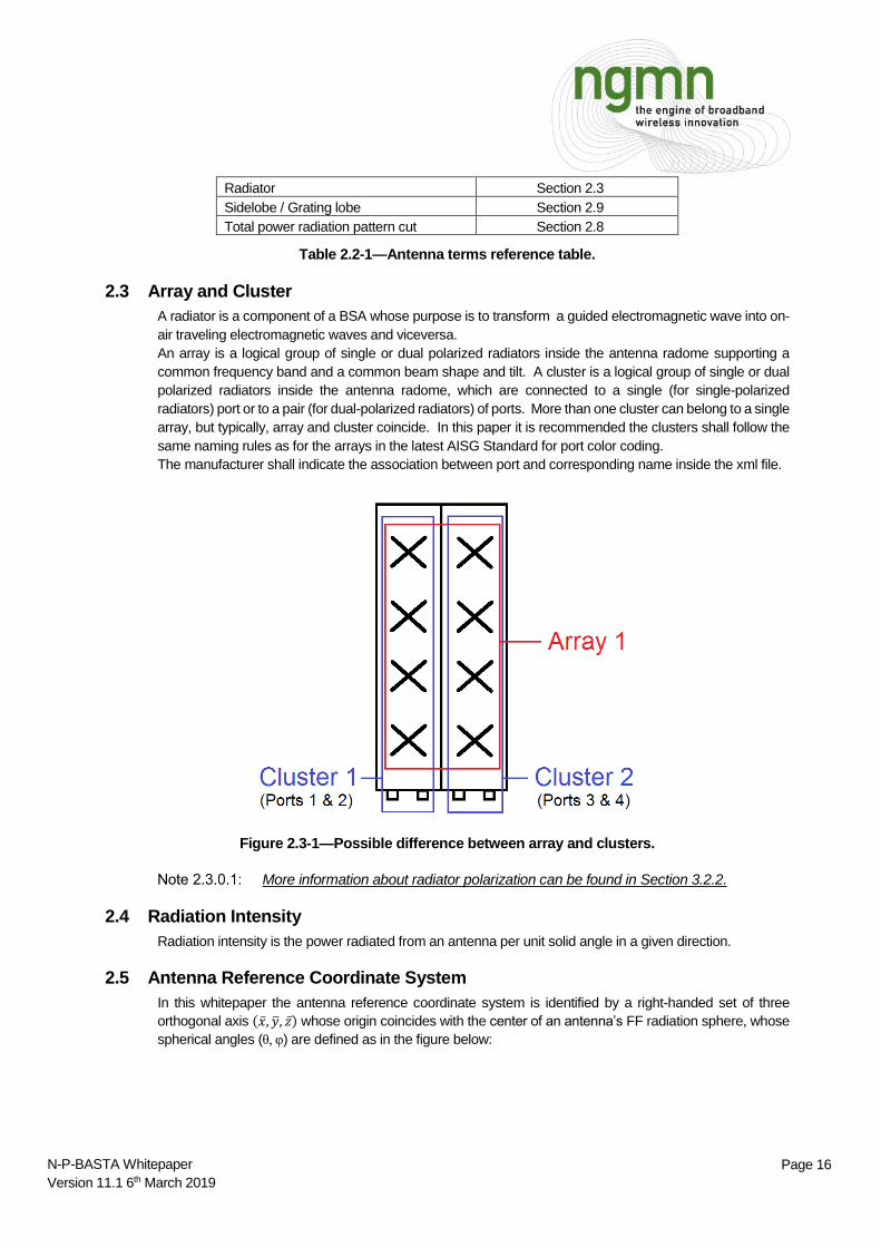
2.3 Array and Cluster
A radiator is a component of a BSA whose purpose is to transform a guided electromagnetic wave into on-
air traveling electromagnetic waves and viceversa.
An array is a logical group of single or dual polarized radiators inside the antenna radome supporting a
common frequency band and a common beam shape and tilt. A cluster is a logical group of single or dual
polarized radiators inside the antenna radome, which are connected to a single (for single-polarized
radiators) port or to a pair (for dual-polarized radiators) of ports. More than one cluster can belong to a single
array, but typically, array and cluster coincide. In this paper it is recommended the clusters shall follow the
same naming rules as for the arrays in the latest AISG Standard for port color coding.
The manufacturer shall indicate the association between port and corresponding name inside the xml file.
Figure 2.3-1—Possible difference between array and clusters.
More information about radiator polarization can be found in Section 3.2.2.
2.4 Radiation Intensity
Radiation intensity is the power radiated from an antenna per unit solid angle in a given direction.
2.5 Antenna Reference Coordinate System
In this whitepaper the antenna reference coordinate system is identified by a right-handed set of three
orthogonal axis (�̅�, �̅�, 𝑧)̅ whose origin coincides with the center of an antenna’s FF radiation sphere, whose
spherical angles (θ, φ) are defined as in the figure below:

t
Page 17 N-P-BASTA Whitepaper
Version 11.1 6th March 2019
Figure 2.5-1—Antenna Reference Coordinate System.
is the angle in the x/y plane, between the x-axis and the projection of the radiating vector onto the x/y
plane and is defined between -180° and +180°, inclusive. is the angle between the projection of the
vector in the x/y plane and the radiating vector and is defined between -90° and +90°, inclusive. Note that
is defined as positive along the down-tilt angle.
Since antennas are produced in different geometries, hence it is impossible to define a universally valid
coordinate system, one or more identifiable antenna physical features shall determine the orientation of its
reference coordinate system. The adopted antenna reference coordinate system shall be explicitly and
unmistakably described from the antenna manufacturer on the BSA’s datasheet (see 11.1.2) and possibly
marked on the antenna. The lack of the two shall indicate that the antenna has a single bidimensional
radiation aperture that is parallel to the �̅�, 𝑧̅ plane, and that the antenna radiates mainly in the semisphere
identified by the �̅� orientation. In this case, the set (�̅�, �̅�, 𝑧)̅ shall also be aligned respectively with the antenna
depth, width and height (see Section 5.1) directions.
Every parameter that needs to refer to a coordinate system will in this document implicitly refer to the antenna
reference coordinate system defined in this section.
2.6 Far-Field Radiation Pattern
The FF radiation pattern (or antenna pattern) is the spatial distribution of the normalized radiation intensity
generated by an antenna in the far-field region. For base station antennas, this region coincides with the
Fraunhofer zone.
2.7 Far-Field Radiation Pattern Cut
The far-field radiation pattern cut is any path on the radiation sphere over which a radiation pattern is
obtained.
z
y
x
ɵ
t
Page 18 N-P-BASTA Whitepaper
Version 11.1 6th March 2019
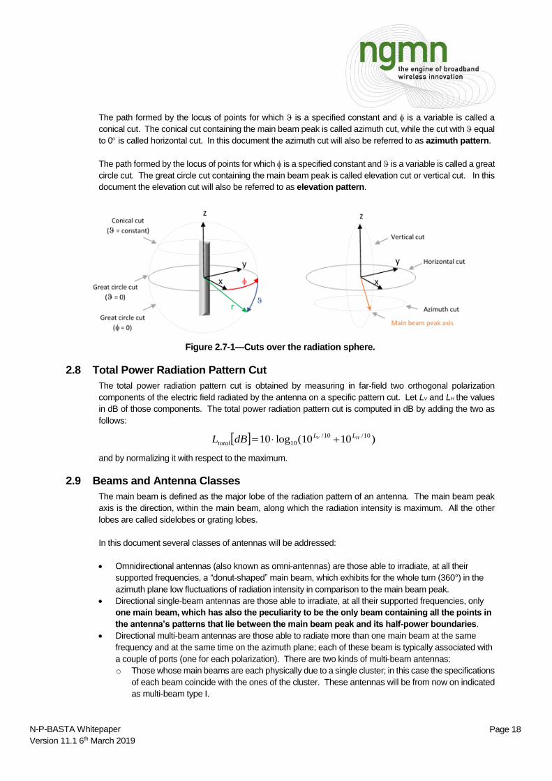
The path formed by the locus of points for which is a specified constant and is a variable is called a
conical cut. The conical cut containing the main beam peak is called azimuth cut, while the cut with equal
to 0 is called horizontal cut. In this document the azimuth cut will also be referred to as azimuth pattern.
The path formed by the locus of points for which is a specified constant and is a variable is called a great
circle cut. The great circle cut containing the main beam peak is called elevation cut or vertical cut. In this
document the elevation cut will also be referred to as elevation pattern.
Figure 2.7-1—Cuts over the radiation sphere.
2.8 Total Power Radiation Pattern Cut
The total power radiation pattern cut is obtained by measuring in far-field two orthogonal polarization
components of the electric field radiated by the antenna on a specific pattern cut. Let LV and LH the values
in dB of those components. The total power radiation pattern cut is computed in dB by adding the two as
follows:
)1010(log1010/10/
10HV LL
total dBL
and by normalizing it with respect to the maximum.
2.9 Beams and Antenna Classes
The main beam is defined as the major lobe of the radiation pattern of an antenna. The main beam peak
axis is the direction, within the main beam, along which the radiation intensity is maximum. All the other
lobes are called sidelobes or grating lobes.
In this document several classes of antennas will be addressed:
Omnidirectional antennas (also known as omni-antennas) are those able to irradiate, at all their
supported frequencies, a “donut-shaped” main beam, which exhibits for the whole turn (360°) in the
azimuth plane low fluctuations of radiation intensity in comparison to the main beam peak.
Directional single-beam antennas are those able to irradiate, at all their supported frequencies, only
one main beam, which has also the peculiarity to be the only beam containing all the points in
the antenna’s patterns that lie between the main beam peak and its half-power boundaries.
Directional multi-beam antennas are those able to radiate more than one main beam at the same
frequency and at the same time on the azimuth plane; each of these beam is typically associated with
a couple of ports (one for each polarization). There are two kinds of multi-beam antennas:
o Those whose main beams are each physically due to a single cluster; in this case the specifications
of each beam coincide with the ones of the cluster. These antennas will be from now on indicated
as multi-beam type I.
t
Page 19 N-P-BASTA Whitepaper
Version 11.1 6th March 2019
o Those whose set of beams can be formed by properly feeding each port and combining each
contribution (e.g.: planar phased-array antennas). In this case there is no physical correspondence
between beam and cluster, and generally each beam is conceptually paired with a pair of ports.
Since it is useful to have specifications for each beam, only as a device those shall be indicated by
associating a cluster to each pair of ports, therefore to each relevant beam. These antennas will
be from now on indicated as multi-beam type II.
Additionally, there is a particular case of multi-beam type II antennas, whose pair of ports cannot be
associated 1:1 to each one of their main beam in the azimuth plane, because a single cluster radiates
more than one of them. Those will be from now on indicated as multi-beam type III.
In this document, in order to identify a common reference to relate antenna parameters to, the axis
perpendicular to the antenna aperture will be called mechanical boresight, and will be used to fulfill that very
purpose. For the purpose of this whitepaper, omni-directional antennas shall have no mechanical boresight.
Parameters normally referring to it will, instead, have the horizon (great circle cut θ = π/2) as reference.
Should the antenna mechanical boresight or horizon not be unmistakably discernible (e.g.: spherical
antenna), a common reference shall be both indicated onto the antenna and specified in its datasheet (see
section 2.5).
Omnidirectional and directional single-beam antennas are basically defined by their
properties, while multi-beam antennas are defined by their use.
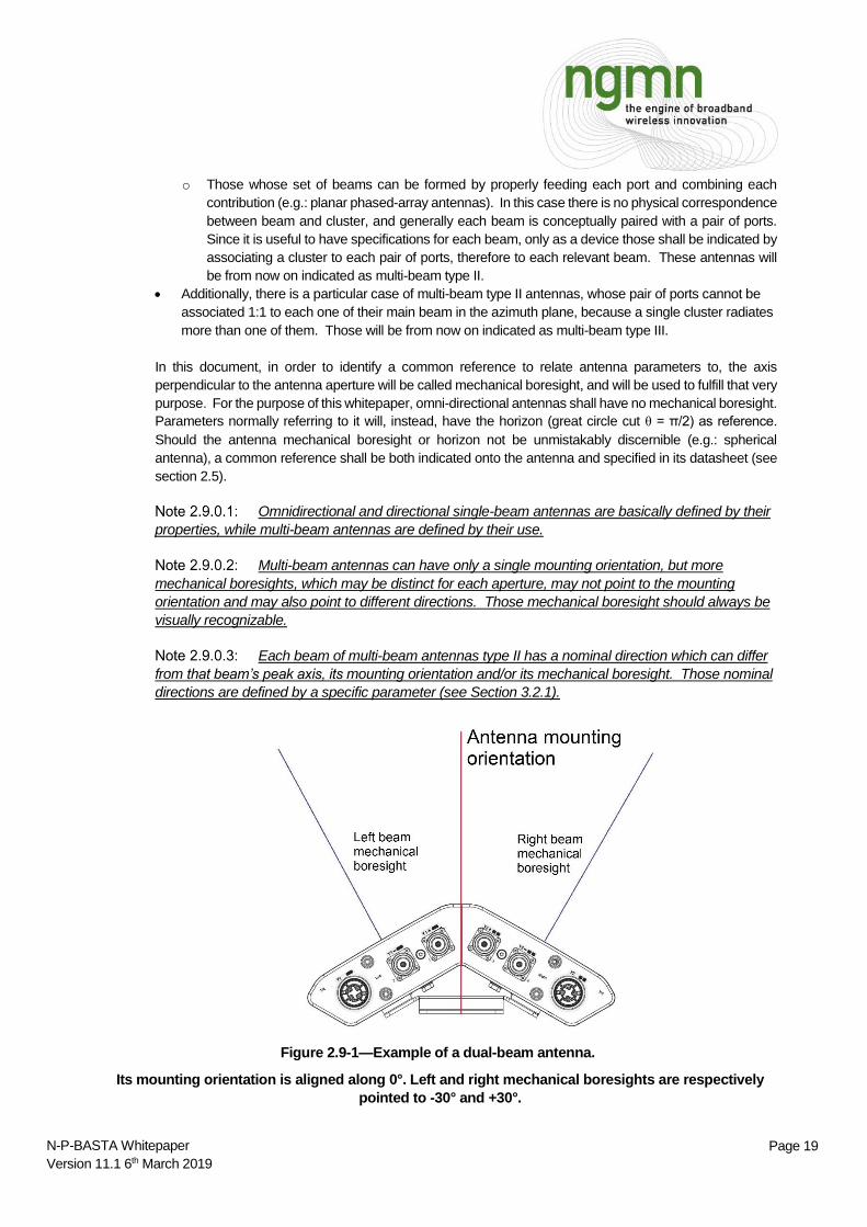
Multi-beam antennas can have only a single mounting orientation, but more
mechanical boresights, which may be distinct for each aperture, may not point to the mounting
orientation and may also point to different directions. Those mechanical boresight should always be
visually recognizable.
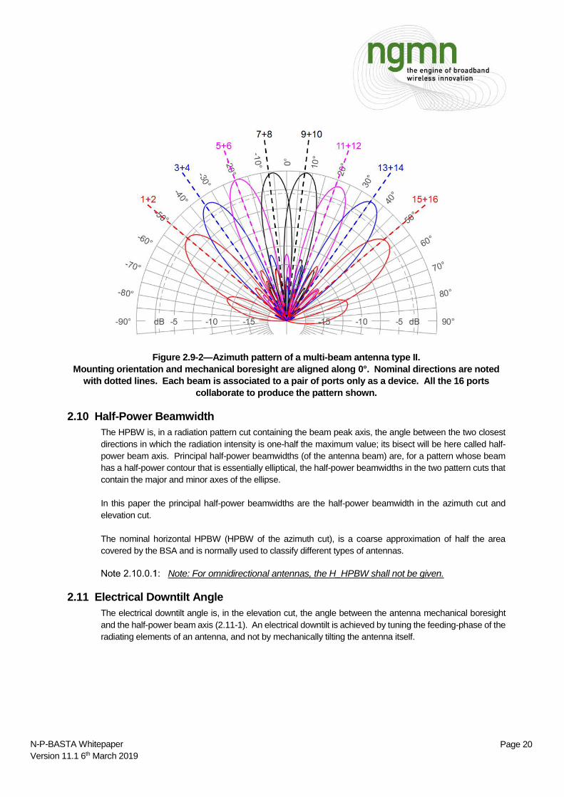
Each beam of multi-beam antennas type II has a nominal direction which can differ
from that beam’s peak axis, its mounting orientation and/or its mechanical boresight. Those nominal
directions are defined by a specific parameter (see Section 3.2.1).
Figure 2.9-1—Example of a dual-beam antenna.
Its mounting orientation is aligned along 0°. Left and right mechanical boresights are respectively
pointed to -30° and +30°.
t
Page 20 N-P-BASTA Whitepaper
Version 11.1 6th March 2019
Figure 2.9-2—Azimuth pattern of a multi-beam antenna type II.
Mounting orientation and mechanical boresight are aligned along 0°. Nominal directions are noted
with dotted lines. Each beam is associated to a pair of ports only as a device. All the 16 ports
collaborate to produce the pattern shown.
2.10 Half-Power Beamwidth
The HPBW is, in a radiation pattern cut containing the beam peak axis, the angle between the two closest
directions in which the radiation intensity is one-half the maximum value; its bisect will be here called half-
power beam axis. Principal half-power beamwidths (of the antenna beam) are, for a pattern whose beam
has a half-power contour that is essentially elliptical, the half-power beamwidths in the two pattern cuts that
contain the major and minor axes of the ellipse.
In this paper the principal half-power beamwidths are the half-power beamwidth in the azimuth cut and
elevation cut.
The nominal horizontal HPBW (HPBW of the azimuth cut), is a coarse approximation of half the area
covered by the BSA and is normally used to classify different types of antennas.
Note: For omnidirectional antennas, the H_HPBW shall not be given.
2.11 Electrical Downtilt Angle
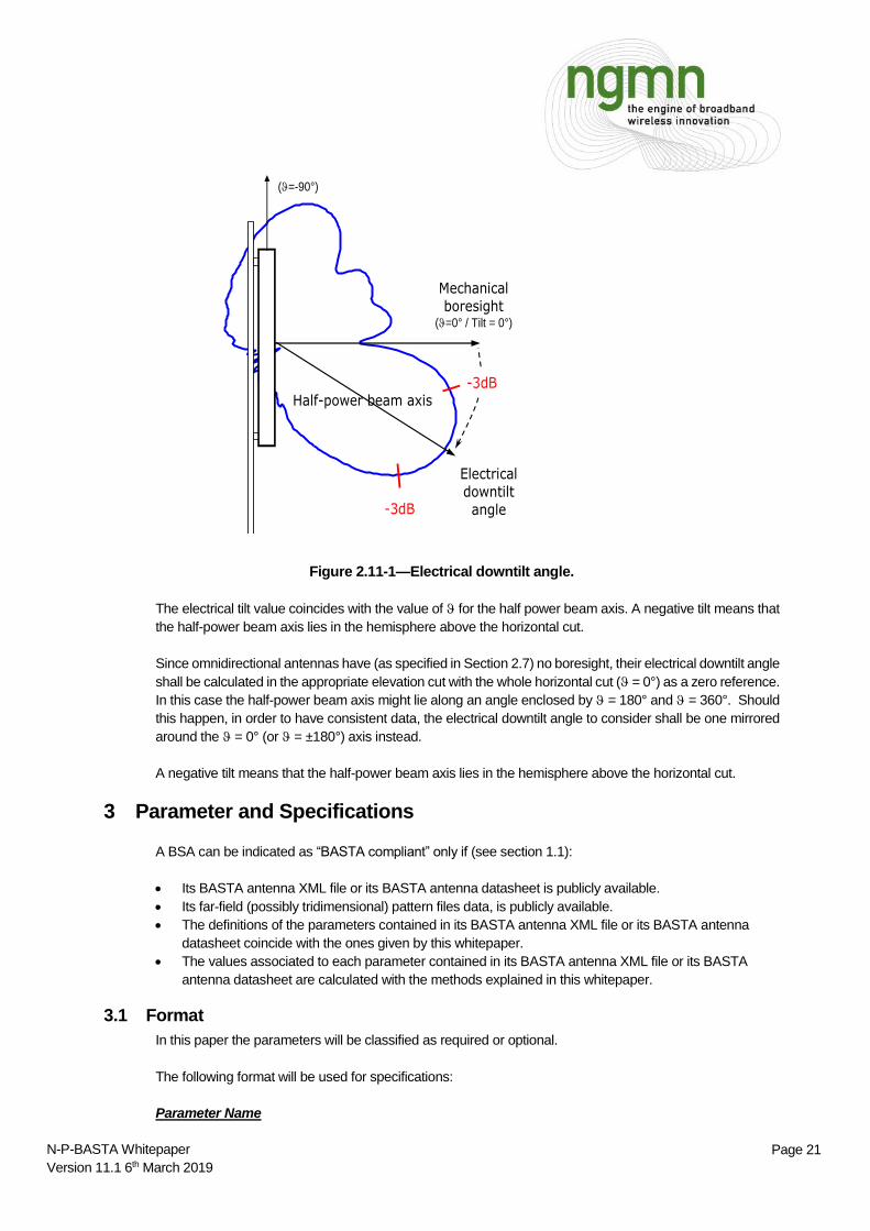
The electrical downtilt angle is, in the elevation cut, the angle between the antenna mechanical boresight
and the half-power beam axis (2.11-1). An electrical downtilt is achieved by tuning the feeding-phase of the
radiating elements of an antenna, and not by mechanically tilting the antenna itself.
t
Page 21 N-P-BASTA Whitepaper
Version 11.1 6th March 2019
80o
90o
100
o
80o
90o
80o
90o
Electrical downtilt angle
Mechanical boresight
(=0° / Tilt = 0°)
Half-power beam axis
(=-90°)
-3dB
-3dB
Figure 2.11-1—Electrical downtilt angle.
The electrical tilt value coincides with the value of for the half power beam axis. A negative tilt means that
the half-power beam axis lies in the hemisphere above the horizontal cut.
Since omnidirectional antennas have (as specified in Section 2.7) no boresight, their electrical downtilt angle
shall be calculated in the appropriate elevation cut with the whole horizontal cut ( = 0°) as a zero reference.
In this case the half-power beam axis might lie along an angle enclosed by = 180° and = 360°. Should
this happen, in order to have consistent data, the electrical downtilt angle to consider shall be one mirrored
around the = 0° (or = ±180°) axis instead.
A negative tilt means that the half-power beam axis lies in the hemisphere above the horizontal cut.
3 Parameter and Specifications
A BSA can be indicated as “BASTA compliant” only if (see section 1.1):
Its BASTA antenna XML file or its BASTA antenna datasheet is publicly available.
Its far-field (possibly tridimensional) pattern files data, is publicly available.
The definitions of the parameters contained in its BASTA antenna XML file or its BASTA antenna
datasheet coincide with the ones given by this whitepaper.
The values associated to each parameter contained in its BASTA antenna XML file or its BASTA
antenna datasheet are calculated with the methods explained in this whitepaper.
3.1 Format
In this paper the parameters will be classified as required or optional.
The following format will be used for specifications:
Parameter Name

t
Page 22 N-P-BASTA Whitepaper
Version 11.1 6th March 2019
Parameter Definition
A description of the parameter in terms of the antenna properties using standard antenna and cellular
communications terminology.
If for any reason it is not possible to describe a particular case with a parameter,
due to the impossibility to fully identify the case within the parameter’s definition, that very parameter
is said to be not applicable.
Specification Definition
A definition for each element of the specification and associated unit of measure.
The specification, if not absolute, will be identified as a nominal or distribution-based (see Sections 4.3
and 4.4).
A description of the specification’s area of validity.
The specification’s measurement unit.
For the purpose of this document, the numeric values associated to each parameter
shall be always positive when not otherwise specified.
Specification Example
An example of the full specification.
XML - Tag Example
Provides an example for the XML tag, in order to show its uniqueness.
If a certain value is only valid in a certain range of the antenna (e.g. frequency range) this is specified
in the cluster section of the XML file.
May provide additional information for the application of the tag.
A tag can contain the optional attribute applicable="false" if the parameter is not applicable.
See also Chapter 10.
For the purpose of this document, the precision of the values associated to each
parameter shall mostly be limited to a single decimal number, even though in some cases an integer
number will suffice. The “XML – Tag Example” sections will always contain an example written with
the correct precision to use in each case.
Relevance
A short description of the impact of the parameter to the antenna performance and/or communication
network performance. Supplementary information may be provided in the additional topics section of
the whitepaper.
If needed, an elaboration on issues surrounding the parameter and its specification will be addressed
here or in the additional topics section of the whitepaper.

t
Page 23 N-P-BASTA Whitepaper
Version 11.1 6th March 2019
A figure illustrating the parameter and specification will be provided where
applicable.
3.2 Required RF Parameters
3.2.1 Antenna Reference, Nominal Sector and Nominal Directions
Parameter Definition
The antenna reference system is identified by a distinctive physical characteristic of the BSA, to which
some other parameters make reference. It is specified in degrees and shall, if necessary, be
indicated on the antenna as well.
The axis along which an antenna is supposed to concentrate the highest peak of radiation is identified
by two angles: the Downtilt Angle in the elevation cut, already defined in section 2.11, and the
Nominal Direction in the azimuth cut.
The angular region equals to two times the nominal horizontal HPBW, which extends symmetrically in
respect to the nominal direction, is the nominal sector (or sector)..
Specification Definition
As stated in section 2.9, for the purpose of this whitepaper the mechanical boresight will be used where
possible to fill the role of antenna reference. Omni-directional antennas shall have no mechanical
boresight, therefore parameters normally referring to it shall, instead, have the horizon (great circle cut
θ = π/2) as reference. Should the antenna mechanical boresight or horizon not be unmistakably
discernible (e.g.: spherical antenna), a reference shall be both indicated onto the antenna and specified
in its datasheet (see section 2.5).
With respect to the antenna reference, the nominal direction is the direction identified in degrees along
the azimuth cut, which the antenna is supposed to concentrate its radiation maximum(s). For a multi-
beam BSA, this parameter shall designate the angles of each beam’s nominal direction.
The antenna sector coarsely defines, in the azimuth cut, the angular aperture in degrees of the area
illuminated by the antenna main beam, or one of the antenna’s main beams.
Specification Example
Type: Nominal Beam 1 Beam 2
Nominal Direction -45° -15°
Nominal Horizontal Half Power Beamwidth 15° 14°
Nominal Sector 30° 28°
XML - Tag Example
<antenna_reference_system alfa="-30” beta=”-20” gamma=”0"/>
<nominal_directions value="-45 ; -15"/>
<nominal_horizontal_half_power_beamwidth value="15; 14"/>
Relevance
On a datasheet, these specifications are valid for one single cluster.
The nominal directions’ tag attribute shall be a string of integer numbers (positive and/or negative),
which shall be separated by the “ ; “ combination of characters.
t
Page 24 N-P-BASTA Whitepaper
Version 11.1 6th March 2019
A 60° nominal horizontal HPBW BSA is expected to have more or less a coverage up to 60°
clockwise and up to 60° counterclockwise in respect to the nominal direction. The 120° angle
included in those boundaries is the sector.
3.2.2 Frequency Range and Frequency Sub-Range
Parameter Definition
The frequency range is the main operating bandwidth of the antenna that is defined by a continuous
range between two limiting frequencies fSTART and fSTOP.
The frequency sub-range (or sub-band) is a specific operating bandwidth included in a frequency range
and defined by a continuous range between two limiting frequencies f´START and f´STOP.
Specification Definition
Ranges are specified in MHz.
Specification Example
Type: Absolute
o Frequency Range 1710-2170 MHz
o Frequency Sub-Range 1710-1880 MHz
XML - Tag Example
<frequency_range start="1710" stop="2170"/>
<frequency_sub_range start="1710" stop="1880">
Relevance
On a datasheet, all specifications valid for the stated frequency range are also valid for its included
frequency sub-bands. Vice versa all specifications valid for the stated frequency sub-range are not
valid outside that very range.
Most BSAs are broadband and they cover one or more frequency sub-range.
See Section 9.1 for an example of cellular frequency sub-bands.
3.2.3 Polarization
Parameter Definition
The nominal polarization associated to the antenna port whose related radiators generate a wave
polarized (nominally) along the same plane.
Specification Definition
The nominal value as a type and direction for the reference polarization of the antenna.
Horizontal and vertical linear polarizations are typically defined as H and V.
Slant linear polarizations are typically defined as +45 and -45.
Circular polarizations are typically defined as RHCP and LHCP.

t
Page 25 N-P-BASTA Whitepaper
Version 11.1 6th March 2019
Specification Example
Type: Nominal 1710-2170 MHz
Polarization Port 1 Port 2
+45 -45
XML - Tag Example
<port name="1" polarization="+45" location=”bottom” connector_type="7-16f"/>
<port name="2" polarization="+45" location=”bottom” connector_type="7-16f"/>
The polarization is provided as a value for a single port and associated to a port’s name.
Relevance
Two orthogonal polarizations are often radiated from an antenna to provide diversity. This is typically
used in uplink and MIMO applications.
Antennas that radiate two orthogonal polarizations are typically called “dual-pol”.
A recommended vendor reference to the polarization labeling convention is described in Section 9.5.
3.2.4 Gain
Parameter Definition
According to the definitions provided by IEEE-145 (1993):
o The antenna gain (in a given direction) is the ratio of the radiation intensity (the power radiated per
unit solid angle), in a given direction, to the radiation intensity that would be obtained if the power
accepted by the antenna were radiated isotropically.
o A realized gain is the gain of an antenna reduced by the losses due to the mismatch of the antenna
input impedance to a specified impedance.
Merely in the interests of simplification, in this document from here on the realized gain will be
addressed as gain.
Specification Definition
Gain is a typical (mean) value in dBi.
It is specified for the specific lowest (minimum), middle, and highest (maximum) downtilt angles of the
whole tilt range for each frequency sub-band.
The gain specified at a certain downtilt angle shall be calculated as the maximum gain of the antenna,
when its downtilt is set to that nominal angle.
In addition, the “over all tilts” gain is specified by a mean value and a tolerance, both over the whole tilt
range and for each frequency sub-band. This is a double-sided distribution-based parameter.
Tolerance is in dB.
Gain validation is determined by the distribution-based methodology described in Section 4.6.
This parameter is to be defined for each frequency sub-band in a broadband antenna. It will be
assumed that the specification is valid for all the ports associated with each frequency sub-band of the
antenna.
The repeatability margin associated with a specified mean gain is defined in Section 4.6 .

t
Page 26 N-P-BASTA Whitepaper
Version 11.1 6th March 2019
A discussion of guidelines for a gain measurement is presented in Section 9.2 and a discussion of the
measurement accuracy that can be expected when measuring gain on a far-field range is discussed in
Section 9.4 .
Specification Example
Type: Distribution-based 1710-1880 MHz 1850-1990 MHz 1920-2170 MHz Gain at 0° Tilt 17.1 17.4 17.7
Gain at 5° Tilt 17.3 17.5 17.7
Gain at 10° Tilt 17.0 17.0 17.2
Over all tilts (0°-10°) 17.2 ± 0.2 17.4 ± 0.3 17.5 ± 0.3
XML - Tag Example
<gain_at_tilt min="17.4" mid="17.5" max="17.0"/>
<gain_over_all_tilts value="17.4" tolerance="0.3"/>
Relevance
Primary specification used in the calculation of a link budget.
The gain specified in radiation pattern data files is used by radio planning software to predict coverage
and capacity performance of a cell.
3.2.5 Gain Ripple
Parameter Definition
For an omnidirectional antenna, gain ripple is the ratio between the peak and the lowest level of the
azimuth pattern.
If the antenna is a single-beam or multi-beam, this parameter shall not be given.
Vice versa, it shall be treated as required for omnidirectional antennas.
Specification Definition
Gain ripple is a maximum value in dB.
It is the difference between the highest and lowest azimuth pattern level, if both are considered in dB.
Pattern levels for this parameter shall be taken with a 1° angular resolution.
It is subject to a distribution-based validation for a single-sided parameter.
This parameter is to be defined for the nominal sub-bands in a broadband antenna. It will be assumed
that the specification is valid for the full electrical downtilt range, and for all the ports associated with
each frequency sub-band of the antenna.
Specification Example
Type: Distribution-based 1710-1880 MHz 1850-1990 MHz 1920-2170 MHz
Gain Ripple < 3.0 < 4.1 < 3.9

t
Page 27 N-P-BASTA Whitepaper
Version 11.1 6th March 2019
XML - Tag Example
<gain_ripple value=”3.2”/>
Relevance
This parameter gives an estimation of the “roundness” of the azimuth pattern.
It is the most characterizing parameter for omni antennas’ radiation in the azimuth plane.
An ideal antenna, which radiates perfectly in every direction in the azimuth plane, would have a gain
ripple of 0.0 dB.
3.2.6 Azimuth Beamwidth
Parameter Definition
The 3 dB (or half-power) azimuth beamwidth of the antenna is defined in the azimuth radiation pattern
as the angular width including the main beam peak, which extends between the only two points at a
beam level 3 dB lower than the maximum of radiation, which are also the nearest to the main beam
peak.
Figure 3.2-1—Calculation of azimuth beamwidth.

t
Page 28 N-P-BASTA Whitepaper
Version 11.1 6th March 2019
Specification Definition
Typical (mean) value in degrees.
Tolerance in degrees.
This is a double-sided distribution-based parameter.
The beamwidth is calculated from the co-polar pattern.
This parameter is to be defined for the nominal sub-bands in a broadband antenna. It will be assumed
that the specification is valid for the full electrical downtilt range, and for all the ports associated with
each frequency sub-band of the antenna.
For omnidirectional antennas, this parameter shall not be given.
Specification Example
Type: Distribution-based 1710-1880 MHz 1850-1990 MHz 1920-2170 MHz
Azimuth Beamwidth 67.9 ± 1.9 65.0 ± 1.6 63.5 ± 2.3
XML - Tag Example
<azimuth_beamwidth value="67.9" tolerance="1.9"/>
Relevance
This beam parameter indicates the sector coverage provided by a BSA.
BSAs are typically referred to by their nominal azimuth beamwidth, for example, a 65° BSA.
Nominal requirements are usually but not limited to, 90° or 65° for 3 sector cell sites, and 45° or 33° for
6 sector sites.
3.2.7 Elevation Beamwidth
Parameter Definition
The 3 dB (or half-power) elevation beamwidth of the antenna is defined in the elevation radiation pattern
as the angular width including the main beam peak, which extends between the only two points at a
beam level 3 dB lower than the maximum of radiation, which are also the nearest to the main beam
peak.
Specification Definition
Typical (mean) value in degrees.
Tolerance in degrees.
This is a double-sided distribution-based parameter.
The beamwidth is calculated from the co-polar pattern.
This parameter is to be defined for the nominal sub-bands in a broadband antenna. It will be assumed
that the specification is valid for the full electrical downtilt range, and for all the ports associated with
each frequency sub-band of the antenna.
Specification Example
Type: Distribution-based 1710-1880 MHz 1850-1990 MHz 1920-2170 MHz
Elevation Beamwidth 7.6 ± 0.4 7.0 ± 0.3 6.6 ± 0.5

t
Page 29 N-P-BASTA Whitepaper
Version 11.1 6th March 2019
XML - Tag Example
<elevation_beamwidth value="6.6" tolerance="0.5"/>
Relevance
One of the parameters contributing to the characteristics and extent of the cell sector coverage.
3.2.8 Electrical Downtilt Range
Parameter Definition
For an antenna capable of variable electrical tilt, the nominal range of angles defined by the minimum
and maximum electrical tilt settings.
For a fixed electrical tilt antenna, the only possible nominal angle.
Specification Definition
For a fixed electrical tilt antenna, the nominal value in degrees.
For a variable electrical tilt antenna, the nominal range of values in degrees.
For omnidirectional antennas, this parameter shall be referenced to the nominal angle between the
horizontal cut and the beam peak axis.
Specification Example
For a variable tilt antenna:
Type: Nominal 1710-2170 MHz
Electrical downtilt 0-10
For a fixed tilt antenna:
Type: Nominal 1710-2170 MHz
Electrical downtilt 4
XML - Tag Example
<electrical_downtilt start="0" stop="10"/>
<electrical_downtilt start="4" stop="4"/>
Relevance
One of the parameters contributing to the characteristics and extent of the cell sector coverage.
The setting of electrical tilt is commonly adjusted for RF coverage and interference optimization.
A parameter that can be adjusted for cell load balancing.
3.2.9 Elevation Downtilt Deviation
Parameter Definition

t
Page 30 N-P-BASTA Whitepaper
Version 11.1 6th March 2019
Maximum deviation of the actual elevation downtilt from the nominal elevation downtilt value.
Specification Definition
Specified as a maximum value in degrees referenced to nominal tilt value.
This is a single-sided distribution-based parameter – its validation is a special case.
It is measured from the Co-Pol pattern.
The reference for the elevation beam peak is the mechanical boresight.
The reference for the nominal tilt setting the elevation downtilt indicator.
Section 4.7 addresses the distribution-based validation of the electrical downtilt deviation.
This parameter is to be defined for the nominal sub-bands in a broadband antenna. It will be assumed
that the specification is valid for the full electrical downtilt range, and for all the ports associated with
each frequency sub-band of the antenna.
For omnidirectional antennas, this parameter shall be referenced to the difference between nominal
and actual angle between the horizontal cut and the beam peak axis.
Specification Example
Type: Distribution-based 1710-1880 MHz 1850-1990 MHz 1920-2170 MHz
Elevation Downtilt Deviation < 0.5 < 0.4 < 0.4
XML - Tag Example
<elevation_downtilt_deviation value="0.5"/>
Relevance
A measure of the accuracy of electrical tilt settings.
3.2.10 Impedance
Parameter Definition
The characteristic impedance is the ratio between voltage and current flowing into an infinite length
transmission line. Validity of this definition is limited to TEM modes (i.e., fundamental modes of coaxial
cable). For an antenna the impedance is defined at its inputs (typically its ports).
Specification Definition
The characteristic impedance nominal value in Ohms.
Specification Example
Type: Nominal 1710-2170 MHz
Impedance 50
XML - Tag Example
<impedance value="50"/>

t
Page 31 N-P-BASTA Whitepaper
Version 11.1 6th March 2019
Relevance
Base station antennas are typically specified to have a characteristic impedance of 50 Ohm.
The VSWR (see below) specification parameter measures the antenna mismatch with respect to
characteristic impedance.
3.2.11 Voltage Standing Wave Ratio
Parameter Definition
The VSWR is defined as the highest ratio between the cluster ports of the maximum and minimum
amplitudes of the voltage standing wave measured at the input ports of an antenna.
Specification Definition
VSWR is an absolute parameter.
Specified as a maximum in-band value without measurement unit. All the possible values lie is between
1 (no reflection) and infinite (total reflection). The reference wave impedance is 50 Ohms.
Specification shall reference the full frequency range, full electrical downtilt range, and associated ports
of the antenna.
Specification Example
Type: Absolute 1710-2170 MHz
Voltage Standing Wave Ratio < 1.5
XML - Tag Example
<vswr value="1.5"/>
Relevance
The VSWR is a measure of the matching of the antenna’s radiators to its source and feeder cables. A
low VSWR will minimize reflections from the antenna.
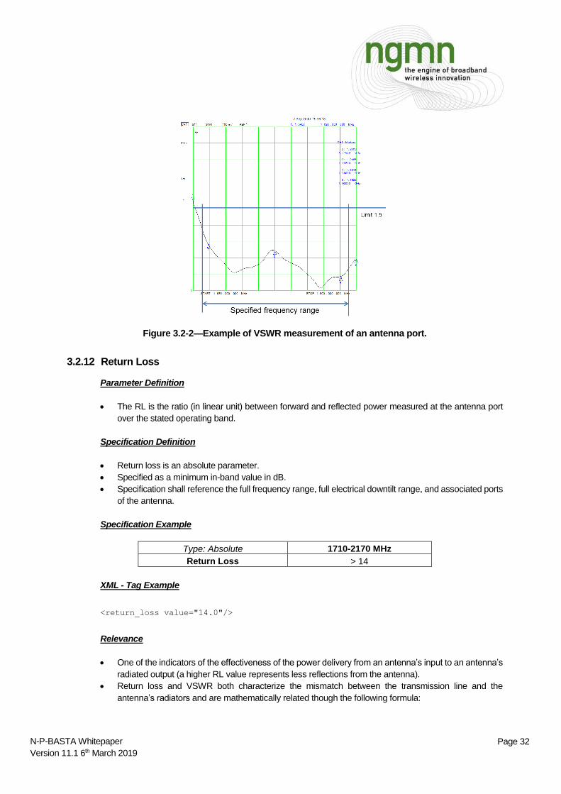
t
Page 32 N-P-BASTA Whitepaper
Version 11.1 6th March 2019
Figure 3.2-2—Example of VSWR measurement of an antenna port.
3.2.12 Return Loss
Parameter Definition
The RL is the ratio (in linear unit) between forward and reflected power measured at the antenna port
over the stated operating band.
Specification Definition
Return loss is an absolute parameter.
Specified as a minimum in-band value in dB.
Specification shall reference the full frequency range, full electrical downtilt range, and associated ports
of the antenna.
Specification Example
Type: Absolute 1710-2170 MHz
Return Loss > 14
XML - Tag Example
<return_loss value="14.0"/>
Relevance
One of the indicators of the effectiveness of the power delivery from an antenna’s input to an antenna’s
radiated output (a higher RL value represents less reflections from the antenna).
Return loss and VSWR both characterize the mismatch between the transmission line and the
antenna’s radiators and are mathematically related though the following formula:

t
Page 33 N-P-BASTA Whitepaper
Version 11.1 6th March 2019
1
1log*20 10
VSWR
VSWRdBRL
Figure 3.2-3—Example of a return loss measurement on a single antenna port.
3.2.13 Intra-Cluster Isolation
Parameter Definition
It is within a cluster the ratio of the power injected in one of the ports associated to a specific polarization,
and the power detected from the other port associated to the polarization orthogonal to the first one.
Figure 3.2-4—Intra-Cluster isolation example: single cluster antenna.

t
Page 34 N-P-BASTA Whitepaper
Version 11.1 6th March 2019
Figure 3.2-5—Intra-Cluster isolation example: dual cluster antenna.
Specification Definition
Intra-Cluster Isolation is a minimum absolute parameter.
Specified in dB.
This parameter is to be defined for all the sub-bands in a broadband antenna. It will be assumed the
specification is for the full electrical downtilt range, and for all the ports associated with each frequency
sub-band of the antenna.
For antennas with multiple dual-pol clusters, the specification applies to each cluster individually and
does not address coupling between them.
Coupling between individual ports is best described in terms of “S parameters”. For example, the
magnitude in dB of the coupling from port 1 to port 2 is signified by S12.
For passive BSAs, coupling is reciprocal, i.e., S12 = S21.
Specification Example
Type: Absolute 1710-1880 MHz 1850-1990 MHz 1920-2170 MHz
Intra-Cluster Isolation > 30 > 28 > 26
XML - Tag Example
<isolation_intra_cluster value="26"/>
Relevance
Coupling between antenna ports can influence the level of filtering required for a given site configuration.
In this dual cluster example, the cross-
polar isolation is the S12 for the first
cluster and S34 for the second cluster.
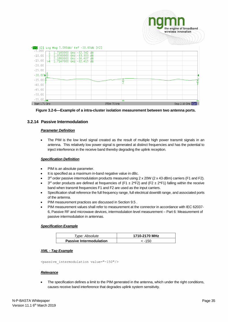
t
Page 35 N-P-BASTA Whitepaper
Version 11.1 6th March 2019
Figure 3.2-6—Example of a intra-cluster isolation measurement between two antenna ports.
3.2.14 Passive Intermodulation
Parameter Definition
The PIM is the low level signal created as the result of multiple high power transmit signals in an
antenna. This relatively low power signal is generated at distinct frequencies and has the potential to
inject interference in the receive band thereby degrading the uplink reception.
Specification Definition
PIM is an absolute parameter.
It is specified as a maximum in-band negative value in dBc.
3rd order passive intermodulation products measured using 2 x 20W (2 x 43 dBm) carriers (F1 and F2).
3rd order products are defined at frequencies of (F1 ± 2*F2) and (F2 ± 2*F1) falling within the receive
band when transmit frequencies F1 and F2 are used as the input carriers.
Specification shall reference the full frequency range, full electrical downtilt range, and associated ports
of the antenna.
PIM measurement practices are discussed in Section 9.5 .
PIM measurement values shall refer to measurement at the connector in accordance with IEC 62037-
6, Passive RF and microwave devices, intermodulation level measurement – Part 6: Measurement of
passive intermodulation in antennas.
Specification Example
Type: Absolute 1710-2170 MHz
Passive Intermodulation < -150
XML - Tag Example
<passive_intermodulation value="-150"/>
Relevance
The specification defines a limit to the PIM generated in the antenna, which under the right conditions,
causes receive band interference that degrades uplink system sensitivity.

t
Page 36 N-P-BASTA Whitepaper
Version 11.1 6th March 2019
3.2.15 Front-to-Back Ratio, Total Power, ± 30°
Parameter Definition
The F/B, total power, ± 30° is defined as the ratio of power gain between the beam peak and the highest
total power value in the 60° angular region of the azimuth cut contained between two boundaries, each
30° distant from the axis corresponding to the nominal direction ± 180°.
Figure 3.2-7—Angular region for front-to-back, total power ± 30° of a 0° nominal direction antenna.
Specification Definition
F/B is specified as a minimum value in dB.
It is subject to a distribution-based validation for a single-sided parameter.
This parameter is to be defined for the nominal sub-bands in a broadband antenna. It will be assumed
that the specification is valid for the full electrical downtilt range, and for all the ports associated with
each frequency sub-band of the antenna.
Section 2.8 addresses the total power calculation.
For omnidirectional antennas, this parameter shall not be given.
Specification Example
Type: Distribution-based 1710-1880 MHz 1850-1990 MHz 1920-2170 MHz
Front-to-Back Ratio, Total Power, ± 30° > 25.0 > 26.4 > 25.8
XML - Tag Example
<front_to_back_ratio_total_power_pm30 value="26.4"/>
Angular region boundary:
nominal direction ± 180° + 30°
Angular region boundary:
nominal direction ± 180° - 30°
Degrees
dB Azimuth Pattern

t
Page 37 N-P-BASTA Whitepaper
Version 11.1 6th March 2019
Relevance
A measure of the interference radiated backwards by the antenna into neighboring cells.
Total power is the root square sum of the linear values of the co-polarized and cross-polarized radiation
from an antenna port.
3.2.16 First Upper Sidelobe Suppression
Parameter Definition
The first upper sidelobe suppression is the gain difference between the main beam peak and the peak
of the closest sidelobe above it.
Figure 3.2-8—First upper sidelobe suppression.
Specification Definition
The gain ratio of the main beam peak and the First Upper SLS must be greater than value in xdB in 84th
percentile of the test samples.
It is subject to a distribution-based validation for a single-sided parameter.
This parameter is to be defined for the nominal sub-bands in a broadband antenna. It will be assumed
that the specification is valid for the full electrical downtilt range, and for all the ports associated with
each frequency sub-band of the antenna.
Sidelobe detection routines are discussed in Section 9.5 .
For omnidirectional antennas, this parameter shall be referenced to the cut by the beam peak axis.
Specification Example
Type: Distribution-based 1710-1880 MHz 1850-1990 MHz 1920-2170 MHz
First Upper Sidelobe Suppression > 18.6 > 17.8 > 16.2
XML - Tag Example
First Upper Sidelobe
dB
Degrees
Main beam peak at
10º electrical tilt
Elevation Pattern

t
Page 38 N-P-BASTA Whitepaper
Version 11.1 6th March 2019
<upper_sidelobe_suppression_first value="18.6"/>
Relevance
Parameter indicating the amount of neighboring cell interference generated by the first sidelobe.
Positioning of the suppressed upper sidelobe using variable electrical tilt can minimize adjacent cell
interference.
3.2.17 Upper Sidelobe Suppression, Peak to 20°
Parameter Definition
The USLS, peak to 20° is the gain difference between the main beam peak and the maximum of the
sidelobes levels in the angular region delimited by the main beam peak and 20 degrees above it.
Figure 3.2-9—Upper sidelobe suppression, peak to 20º.
Specification Definition
Upper SLS from main beam peak to 20° above the main peak must be less than value in xxdB in 84th
percentile of the test samples.
It is subject to a distribution-based validation for a single-sided parameter.
This parameter is to be defined for the nominal sub-bands in a broadband antenna. It will be assumed
that the specification is valid for the full electrical downtilt range, and for all the ports associated with
each frequency sub-band of the antenna.
Sidelobe detection routines are discussed in Section 9.5 .
For omnidirectional antennas, this parameter shall be referenced to the cut by the beam peak axis.
Angular region of specification -
20° above the main beam peak
Main beam peak at
10º electrical tilt
Degrees
dB
Elevation Pattern

t
Page 39 N-P-BASTA Whitepaper
Version 11.1 6th March 2019
Specification Example
Type: Distribution-based 1710-1880 MHz 1850-1990 MHz 1920-2170 MHz
Upper Sidelobe Suppression, Peak to 20° > 18.6 > 17.8 > 16.2
XML - Tag Example
<upper_sidelobe_suppression_peak_to_20 value="16.2"/>
Relevance
Parameter indicating the amount of neighboring cell interference generated by the upper sidelobes.
Positioning of the suppressed upper sidelobes using variable electrical tilt can minimize adjacent-cell
interference.
3.2.18 Cross-Polar Discrimination over Sector
Parameter Definition
The CPD over sector is defined as the lowest ratio between the co-polar component of a specific
polarization and the orthogonal cross-polar component (typically +45° to -45° or vice versa) within the
left and right sector boundaries in respect to the projection of the mechanical boresight onto the azimuth
cut.
Figure 3.2-10—Cross-polar discrimination over sector of a 0° mechanical boresight, 60° nominal
horizontal HPBW antenna.
Specification Definition
Sector boundary
CPD at a given angle
Co-pol pattern
dB
Degrees
Cross-pol pattern

t
Page 40 N-P-BASTA Whitepaper
Version 11.1 6th March 2019
CPD is the magnitude of the relative power of the Co-Pol pattern with respect to the Cr-Pol pattern at a
given angle.
The CPD over the sector is the worst case measured in a defined angular deviation from the main beam
direction. It will be assumed that the parameter is referenced to the nominal sector associated with the
antenna.
It is subject to a distribution-based validation for a single-sided parameter.
For a three sector application the nominal sector is normally defined as 120°. For a six sector application
the nominal sector is normally defined 60°.
This parameter is to be defined for the nominal sub-bands in a broadband antenna. It will be assumed
that the specification is valid for the full electrical downtilt range, and for all the ports associated with
each frequency sub-band of the antenna.
For multi-beam antennas type II, this parameter shall be instead defined for each beam as the CPR
over the nominal beamwidth of the analyzed beam around the projection of its nominal direction onto
the azimuth cut.
For omnidirectional antennas, this parameter shall be referenced to the whole turn. It shall then be the
worst possible case.
Specification Example
Type: Distribution-based 1710-1880 MHz 1850-1990 MHz 1920-2170 MHz
Cross Polar Discrimination Over Sector > 10.8 > 9.4 > 8.5
XML - Tag Example
<cross_polar_discrimination_over_sector value="10.8"/>
Relevance
CPD is important for a low level of correlation between the orthogonally polarized propagation channels.
Correlation generated by the antenna can negatively affect receive diversity and MIMO performance of
the system.
3.2.19 Maximum Effective Power per Port
Parameter Definition
The maximum power, which can be transmitted into one antenna port, and does not cause any damage
to the antenna or negatively affect the antenna mechanical or electrical integrity and performance
(hence subject to parameters’ alteration).
Specification Definition
Power is defined as effective CW power.
This is an absolute, maximum parameter specified in Watts.
It is valid for the operational environmental conditions specified for the antenna.
Specification shall reference the full frequency range, full electrical downtilt range, and associated ports
of the antenna.
Specification Example

t
Page 41 N-P-BASTA Whitepaper
Version 11.1 6th March 2019
Type: Absolute 1710-2170 MHz
Maximum Effective Power per Port 250
XML - Tag Example
<maximum_effective_power_per_port value="250"/>
Relevance
Exceeding the specified power rating can damage the antenna.
3.2.20 Maximum Effective Power Whole Antenna
Parameter Definition
The maximum power, which can be transmitted into the antenna, and does not cause any damage to
the antenna or negatively affect the antenna mechanical or electrical integrity and performance (hence
subject to parameters’ alteration).
Specification Definition
Power is defined as effective CW power.
This is an absolute, maximum parameter specified in Watts.
It is valid for the operational environmental conditions specified for the antenna.
Specification shall reference all the frequency ranges, the full electrical downtilt range, and all the ports
of the antenna.
Specification Example
Type: Absolute
Maximum Effective Power Whole Antenna 1200
XML - Tag Example
<maximum_effective_power_antenna value="1200"/>
Relevance
Exceeding the specified power rating can damage the antenna.
3.2.21 Inter-Cluster Isolation
Parameter Definition
The worst coupling case between a port of a specific cluster and any other port of another cluster in a
multiple band, or broad band antenna.
Specification Definition
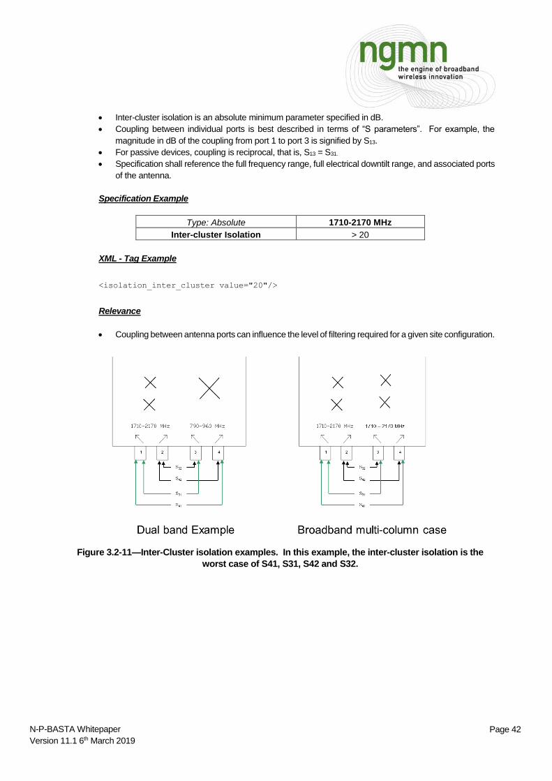
t
Page 42 N-P-BASTA Whitepaper
Version 11.1 6th March 2019
Inter-cluster isolation is an absolute minimum parameter specified in dB.
Coupling between individual ports is best described in terms of “S parameters”. For example, the
magnitude in dB of the coupling from port 1 to port 3 is signified by S13.
For passive devices, coupling is reciprocal, that is, S13 = S31.
Specification shall reference the full frequency range, full electrical downtilt range, and associated ports
of the antenna.
Specification Example
Type: Absolute 1710-2170 MHz
Inter-cluster Isolation > 20
XML - Tag Example
<isolation_inter_cluster value="20"/>
Relevance
Coupling between antenna ports can influence the level of filtering required for a given site configuration.
Figure 3.2-11—Inter-Cluster isolation examples. In this example, the inter-cluster isolation is the
worst case of S41, S31, S42 and S32.
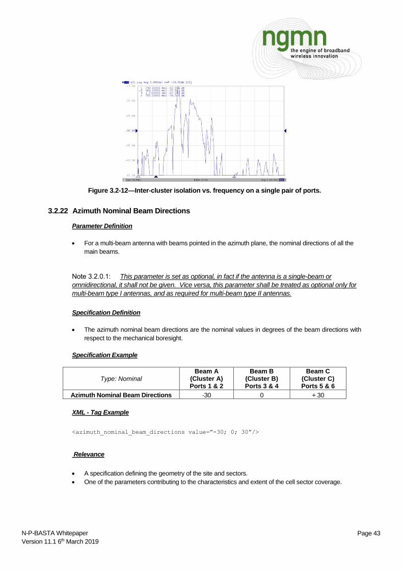
t
Page 43 N-P-BASTA Whitepaper
Version 11.1 6th March 2019
Figure 3.2-12—Inter-cluster isolation vs. frequency on a single pair of ports.
3.2.22 Azimuth Nominal Beam Directions
Parameter Definition
For a multi-beam antenna with beams pointed in the azimuth plane, the nominal directions of all the
main beams.
This parameter is set as optional, in fact if the antenna is a single-beam or
omnidirectional, it shall not be given. Vice versa, this parameter shall be treated as optional only for
multi-beam type I antennas, and as required for multi-beam type II antennas.
Specification Definition
The azimuth nominal beam directions are the nominal values in degrees of the beam directions with
respect to the mechanical boresight.
Specification Example
Type: Nominal Beam A
(Cluster A) Ports 1 & 2
Beam B (Cluster B) Ports 3 & 4
Beam C (Cluster C) Ports 5 & 6
Azimuth Nominal Beam Directions -30 0 + 30
XML - Tag Example
<azimuth_nominal_beam_directions value=”-30; 0; 30”/>
Relevance
A specification defining the geometry of the site and sectors.
One of the parameters contributing to the characteristics and extent of the cell sector coverage.

t
Page 44 N-P-BASTA Whitepaper
Version 11.1 6th March 2019
3.3 Optional RF Parameters
3.3.1 Azimuth Beam Squint
Parameter Definition
The azimuth beam squint is the difference in the azimuth cut between the pointing direction of the main
beam and the antenna’s nominal direction. The pointing direction of the main beam is defined as the
half-power beamwidth bisect.
Figure 3.3-1—Illustration of beam squint calculation for a given frequency, tilt and port.
Specification Definition
Typical (mean) value in degrees.
Tolerance in degrees.
It is subject to a distribution-based validation for a double-sided parameter.
Squint is measured from the co-polar pattern.
This parameter is to be defined for the nominal sub-bands in a broadband antenna. It will be assumed
that the specification is valid for the full electrical downtilt range, and for all the ports associated with
each frequency sub-band of the antenna.
For multi-beam antennas type II, this parameter shall be instead defined for each beam, as the
difference in the azimuth cut between the pointing direction (defined as the half-power beamwidth
bisect) of the analyzed beam and its nominal direction.
For omnidirectional antennas, this parameter shall not be given.
Specification Example
dB
Degrees -28.6° +37.8°
+4.6°
Beam Squint
33.2° 33.2°
Left port, 0°, 1.85 GHz
Center of the 3 dB Beamwidth
0° is the nominal direction of the antenna
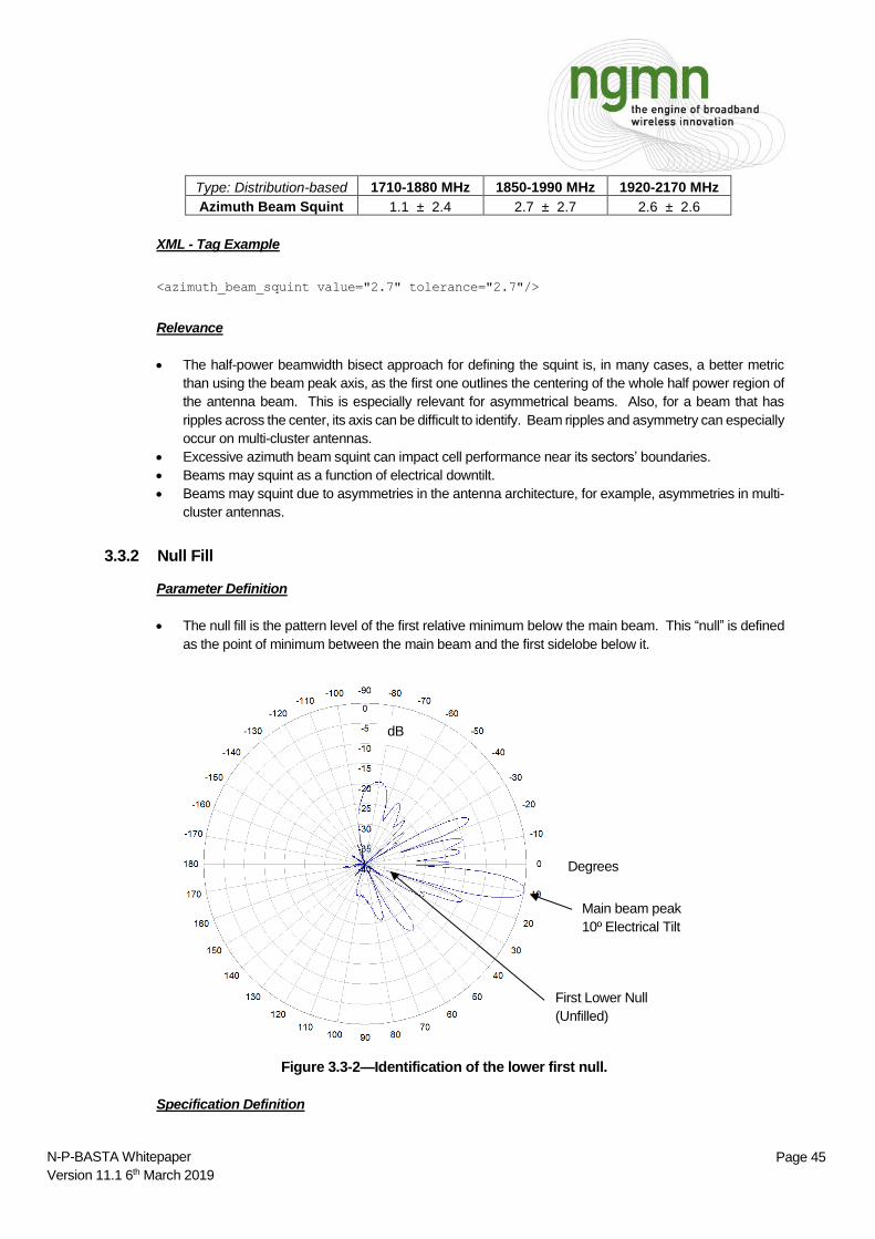
t
Page 45 N-P-BASTA Whitepaper
Version 11.1 6th March 2019
Type: Distribution-based 1710-1880 MHz 1850-1990 MHz 1920-2170 MHz
Azimuth Beam Squint 1.1 ± 2.4 2.7 ± 2.7 2.6 ± 2.6
XML - Tag Example
<azimuth_beam_squint value="2.7" tolerance="2.7"/>
Relevance
The half-power beamwidth bisect approach for defining the squint is, in many cases, a better metric
than using the beam peak axis, as the first one outlines the centering of the whole half power region of
the antenna beam. This is especially relevant for asymmetrical beams. Also, for a beam that has
ripples across the center, its axis can be difficult to identify. Beam ripples and asymmetry can especially
occur on multi-cluster antennas.
Excessive azimuth beam squint can impact cell performance near its sectors’ boundaries.
Beams may squint as a function of electrical downtilt.
Beams may squint due to asymmetries in the antenna architecture, for example, asymmetries in multi-
cluster antennas.
3.3.2 Null Fill
Parameter Definition
The null fill is the pattern level of the first relative minimum below the main beam. This “null” is defined
as the point of minimum between the main beam and the first sidelobe below it.
Figure 3.3-2—Identification of the lower first null.
Specification Definition
First Lower Null
(Unfilled)
dB
Degrees
Main beam peak
10º Electrical Tilt

t
Page 46 N-P-BASTA Whitepaper
Version 11.1 6th March 2019
Null fill is a minimum value in dB.
It is subject to a distribution-based validation for a single-sided parameter.
This parameter is to be defined for the nominal sub-bands in a broadband antenna. It will be assumed
that the specification is valid for the full electrical downtilt range, and for all the ports associated with
each frequency sub-band of the antenna.
Since the null fill depends from the first lower sidelobe, its detection routines are discussed with the
sidelobes’ ones in Section 9.5 .
For omnidirectional antennas, this parameter shall be referenced to the cut by the beam peak axis.
Specification Example
Type: Distribution-based 1710-1880 MHz 1850-1990 MHz 1920-2170 MHz
Null Fill < 30.2 < 30.3 < 30.3
XML - Tag Example
<null_fill value="30.2"/>
Relevance
Null fill is, in most BSA site scenarios, a non-critical parameter due multipath in the environment and
power levels near the cell site.
Pattern shaping methods are sometimes applied to fill the lower null.
It can affect the coverage close to base stations with high antenna positions where the null illumination
may fall on distances from the antenna where the path loss is sufficient to create coverage holes, and
scattering is insufficient to create secondary illumination from the lobes..
3.3.3 Cross-Polar Discrimination at Mechanical boresight
Parameter Definition
The CPD at mechanical boresight is defined as the ratio of the azimuthal Co-Pol component of a specific
polarization to the orthogonal Cr-Pol component (typically +45° to -45° or vice versa) along the
projection of the mechanical boresight onto the azimuth cut.

t
Page 47 N-P-BASTA Whitepaper
Version 11.1 6th March 2019
Figure 3.3-3—Cross-polar discrimination at mechanical boresight.
Specification Definition
CPD at mechanical boresight is specified as a minimum value in dB in 84th percentile of the test
samples.
It is subject to a distribution-based validation for a single-sided parameter.
This parameter is to be defined for the nominal sub-bands in a broadband antenna. It will be assumed
that the specification is valid for the full electrical downtilt range, and for all the ports associated with
each frequency sub-band of the antenna.
For multi-beam antennas type II, this parameter shall be instead defined for each beam, as the CPR of
the analyzed beam in respect to the projection of its nominal direction onto the azimuth cut.
For omnidirectional antennas, this parameter shall not be given.
Specification Example
Type: Distribution-based 1710-1880 MHz 1850-1990 MHz 1920-2170 MHz
Cross Polar Discrimination at Mechanical boresight > 25.4 > 22.1 > 26.3
XML - Tag Example
<cross_polar_discrimination_at_mechanical_boresight value="25.4"/>
Relevance
CPD is important for a low level of correlation between the orthogonally polarized propagation channels.
Correlation generated by the antenna can negatively affect receive diversity and MIMO downlink
performance of the system.
CPD at boresight
Co-pol pattern
dB
Degrees
Cross-pol pattern

t
Page 48 N-P-BASTA Whitepaper
Version 11.1 6th March 2019
3.3.4 Cross-Polar Discrimination over 3 dB Azimuth Beamwidth
Parameter Definition
The CPD over 3 dB azimuth beamwidth is defined as the lowest ratio between the co-polar component
of a specific polarization and the orthogonal cross-polar component (typically +45° to -45° or vice versa)
within the half-power angular region (between the -3 dB levels of the antenna pattern nearest to the
beam peak) in the azimuth cut.
Figure 3.3-4—Cross pol discrimination over 3 dB azimuth beamwidth.
Specification Definition
CPD over 3 dB azimuth beamwidth is specified as a minimum value in dB.
It is subject to a distribution-based validation for a single-sided parameter.
This parameter is to be defined for the nominal sub-bands in a broadband antenna. It will be assumed
that the specification is valid for the full electrical downtilt range, and for all the ports associated with
each frequency sub-band of the antenna.
For omnidirectional antennas, this parameter shall not be given.
Specification Example
Type: Distribution-based 1710-1880 MHz 1850-1990 MHz 1920-2170 MHz
Cross-Polar Discrimination over 3 dB Azimuth Beamwidth > 11.8 > 16.3 > 14.6
XML - Tag Example
<cross_polar_discrimination_over_3_db_azimuth_beamwidth value="XXX"/>
-3 dB angular region
Co-Pol pattern
dB
Degrees
Cr-pol pattern

t
Page 49 N-P-BASTA Whitepaper
Version 11.1 6th March 2019
Relevance
CPD is important for a low level of correlation between the orthogonally polarized propagation channels.
Correlation generated by the antenna can negatively affect receive diversity and MIMO downlink
performance of the system.
3.3.5 Cross-Polar Discrimination over 10 dB Azimuth Beamwidth
Parameter Definition
The CPD over 10 dB azimuth beamwidth is defined as the lowest ratio between the co-polar component
of a specific polarization and the orthogonal cross-polar component (typically +45° to -45° or vice versa)
within the half-power angular region (between the -10 dB levels of the antenna pattern nearest to the
beam peak) in the azimuth cut.
Figure 3.3-5—Cross pol discrimination over 10 dB azimuth beamwidth.
Specification Definition
CPD over 10 dB azimuth beamwidth is specified as a minimum value in dB.
It is subject to a distribution-based validation for a single-sided parameter.
This parameter is to be defined for the nominal sub-bands in a broadband antenna. It will be assumed
that the specification is valid for the full electrical downtilt range, and for all the ports associated with
each frequency sub-band of the antenna.
For omnidirectional antennas, this parameter shall not be given.
Specification Example
-10 dB angular region
Co-Pol pattern
dB
Degrees
Cross-Pol pattern
t
Page 50 N-P-BASTA Whitepaper
Version 11.1 6th March 2019
Type: Distribution-based 1710-1880 MHz 1850-1990 MHz 1920-2170 MHz
Cross Polar Discrimination over 10 dB Beamwidth > 11.8 > 13.4 > 12.2
XML - Tag Example
<cross_polar_discrimination_over_10_db_beamwidth value="11.8"/>
Relevance
o CPD is important for a low level of correlation between the orthogonally polarized propagation channels.
Correlation generated by the antenna can negatively affect receive diversity and MIMO downlink
performance of the system.
3.3.6 Cross Polar Discrimination over 3 dB Elevation Beamwidth
Parameter Definition
The CPD over 3 dB elevation beamwidth is defined as the lowest ratio between the co-polar component
of a specific polarization and the orthogonal cross-polar component (typically +45° to -45° or vice versa)
within the half-power angular region (between the -3 dB levels of the antenna pattern nearest to the
beam peak) in the elevation cut.
Specification Definition
CPD over the 3 dB elevation beamwidth is specified as a minimum value in dB.
It is subject to a distribution-based validation for a single-sided parameter.
This parameter is to be defined for the nominal sub-bands in a broadband antenna. It will be assumed
that the specification is valid for the full electrical downtilt range, and for all the ports associated with
each frequency sub-band of the antenna.
For omnidirectional antennas, this parameter shall be referenced to the cut by the beam peak axis.
Specification Example
Type: Distribution-based 1710-1880 MHz 1850-1990 MHz 1920-2170 MHz
Cross Polar Discrimination over the 3 dB Elevation Beamwidth > 11.3 > 10.7 > 9.8
XML - Tag Example
<cross_polar_discrimination_over_3_db_elevation_beamwidth value="11.3"/>
Relevance
CPD is important for a low level of correlation between the orthogonally polarized propagation channels.
Correlation generated by the antenna can negatively affect receive diversity and MIMO downlink
performance of the system.
t
Page 51 N-P-BASTA Whitepaper
Version 11.1 6th March 2019
3.3.7 Cross Polar Discrimination over 10 dB Elevation Beamwidth
Parameter Definition
The CPD over 10 dB elevation beamwidth is defined as the lowest ratio between the co-polar
component of a specific polarization and the orthogonal cross-polar component (typically +45° to -45°
or vice versa) within the half-power angular region (between the -10 dB levels of the antenna pattern
nearest to the beam peak) in the elevation cut.
Specification Definition
CPD over the 10 dB elevation beamwidth is specified as a minimum value in dB.
It is subject to a distribution-based validation for a single-sided parameter.
This parameter is to be defined for the nominal sub-bands in a broadband antenna. It will be assumed
that the specification is valid for the full electrical downtilt range, and for all the ports associated with
each frequency sub-band of the antenna.
For omnidirectional antennas, this parameter shall be referenced to the cut by the beam peak axis.
Specification Example
Type: Distribution-based 1710-1880 MHz 1850-1990 MHz 1920-2170 MHz
Cross Polar Discrimination over the 10 dB Elevation Beamwidth > 11.0 > 10.2 > 9.8
XML - Tag Example
<cross_polar_discrimination_over_10_db_elevation_beamwidth value="11.0"/>
Relevance
CPD is important for a low level of correlation between the orthogonally polarized propagation channels.
Correlation generated by the antenna can negatively affect receive diversity and MIMO downlink
performance of the system.
3.3.8 Azimuth Beam Port-to-Port Tracking
Parameter Definition
Azimuth beam port-to-port tracking is the highest ratio between the amplitude of the two antenna Co-
Pol polarization branches (e.g.: +45° by port 1 to -45° by port 2) within the sector boundaries.
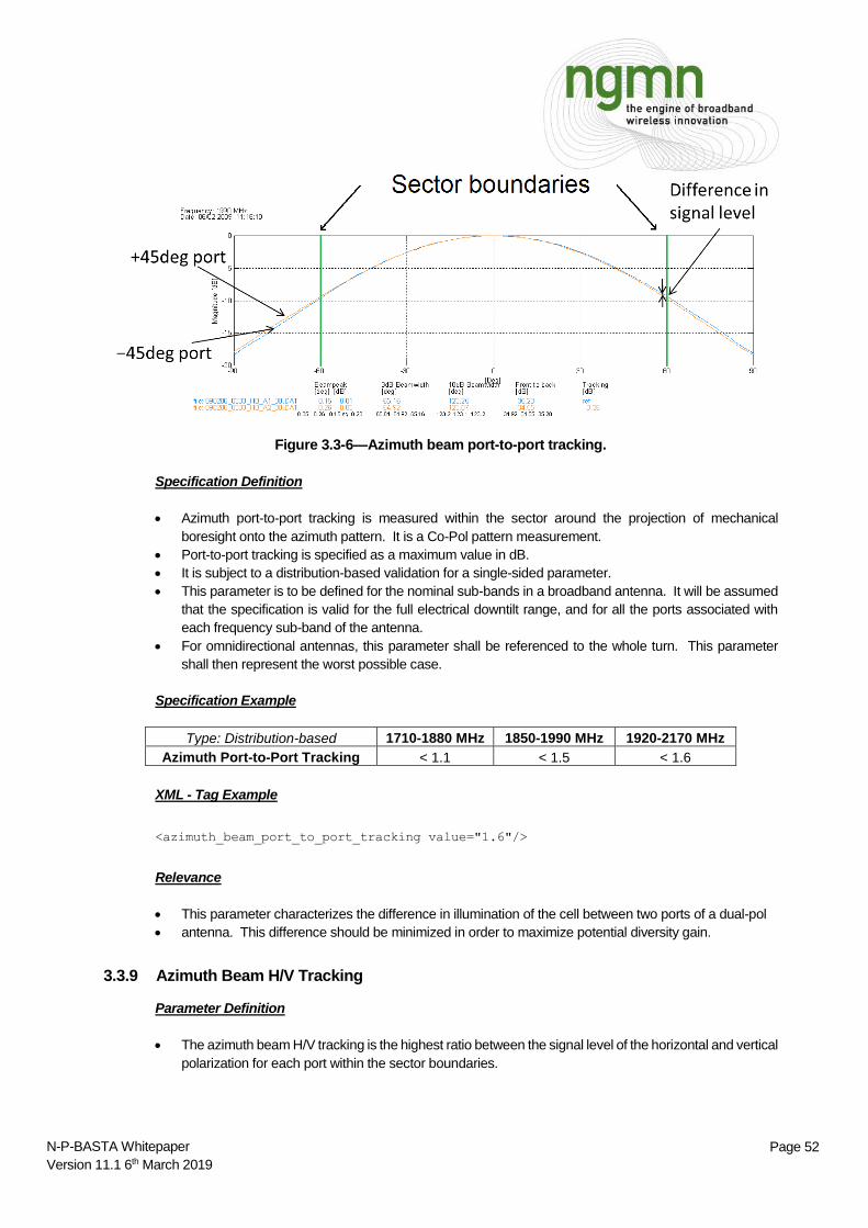
t
Page 52 N-P-BASTA Whitepaper
Version 11.1 6th March 2019
Figure 3.3-6—Azimuth beam port-to-port tracking.
Specification Definition
Azimuth port-to-port tracking is measured within the sector around the projection of mechanical
boresight onto the azimuth pattern. It is a Co-Pol pattern measurement.
Port-to-port tracking is specified as a maximum value in dB.
It is subject to a distribution-based validation for a single-sided parameter.
This parameter is to be defined for the nominal sub-bands in a broadband antenna. It will be assumed
that the specification is valid for the full electrical downtilt range, and for all the ports associated with
each frequency sub-band of the antenna.
For omnidirectional antennas, this parameter shall be referenced to the whole turn. This parameter
shall then represent the worst possible case.
Specification Example
Type: Distribution-based 1710-1880 MHz 1850-1990 MHz 1920-2170 MHz
Azimuth Port-to-Port Tracking < 1.1 < 1.5 < 1.6
XML - Tag Example
<azimuth_beam_port_to_port_tracking value="1.6"/>
Relevance
This parameter characterizes the difference in illumination of the cell between two ports of a dual-pol
antenna. This difference should be minimized in order to maximize potential diversity gain.
3.3.9 Azimuth Beam H/V Tracking
Parameter Definition
The azimuth beam H/V tracking is the highest ratio between the signal level of the horizontal and vertical
polarization for each port within the sector boundaries.
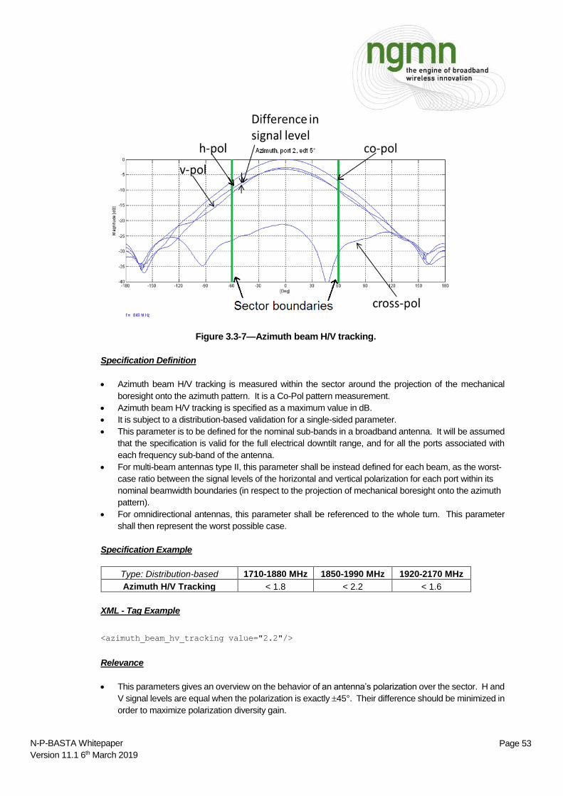
t
Page 53 N-P-BASTA Whitepaper
Version 11.1 6th March 2019
Figure 3.3-7—Azimuth beam H/V tracking.
Specification Definition
Azimuth beam H/V tracking is measured within the sector around the projection of the mechanical
boresight onto the azimuth pattern. It is a Co-Pol pattern measurement.
Azimuth beam H/V tracking is specified as a maximum value in dB.
It is subject to a distribution-based validation for a single-sided parameter.
This parameter is to be defined for the nominal sub-bands in a broadband antenna. It will be assumed
that the specification is valid for the full electrical downtilt range, and for all the ports associated with
each frequency sub-band of the antenna.
For multi-beam antennas type II, this parameter shall be instead defined for each beam, as the worst-
case ratio between the signal levels of the horizontal and vertical polarization for each port within its
nominal beamwidth boundaries (in respect to the projection of mechanical boresight onto the azimuth
pattern).
For omnidirectional antennas, this parameter shall be referenced to the whole turn. This parameter
shall then represent the worst possible case.
Specification Example
Type: Distribution-based 1710-1880 MHz 1850-1990 MHz 1920-2170 MHz
Azimuth H/V Tracking < 1.8 < 2.2 < 1.6
XML - Tag Example
<azimuth_beam_hv_tracking value="2.2"/>
Relevance
This parameters gives an overview on the behavior of an antenna’s polarization over the sector. H and
V signal levels are equal when the polarization is exactly 45°. Their difference should be minimized in
order to maximize polarization diversity gain.

t
Page 54 N-P-BASTA Whitepaper
Version 11.1 6th March 2019
3.3.10 Azimuth Beam Roll-Off
Parameter Definition
The azimuth beam roll-off is highest difference of the Co-Pol signal levels at the sector edges in respect
to the one at the main beam peak.
Figure 3.3-8—Azimuth beam roll-off.
Specification Definition
Azimuth beam roll-off is defined as the combination of a typical (mean) value and a tolerance, both in
dB.
It is subject to a distribution-based validation for a double-sided parameter.
It is measured at the sector edges around the projection of the mechanical boresight onto the azimuth
pattern. It is a Co-Pol pattern measurement.
This parameter is to be defined for the nominal sub-bands in a broadband antenna. It will be assumed
that the specification is valid for the full electrical downtilt range, for all the ports associated with each
frequency sub-band of the antenna and for both the sector edges.
For multi-beam antennas type II, this parameter shall be instead defined for each beam, the signal
level at the nominal beamwidth edges (in respect to the projection of mechanical boresight onto the
azimuth pattern) of the two antenna Co-Pol polarization branches of the analyzed beam.
For omnidirectional antennas, this parameter shall not be given.
Specification Example
Type: Distribution-based 1710-1880 MHz 1850-1990 MHz 1920-2170 MHz
Azimuth Beam Roll-Off 8.1 ± 1.6 9.8 ± 2.3 11.3 ± 2.1
XML - Tag Example
<azimuth_beam_roll_off value="11.3" tolerance="2.1"/>
Relevance
Sector edges
8.4 dB 7.6 dB
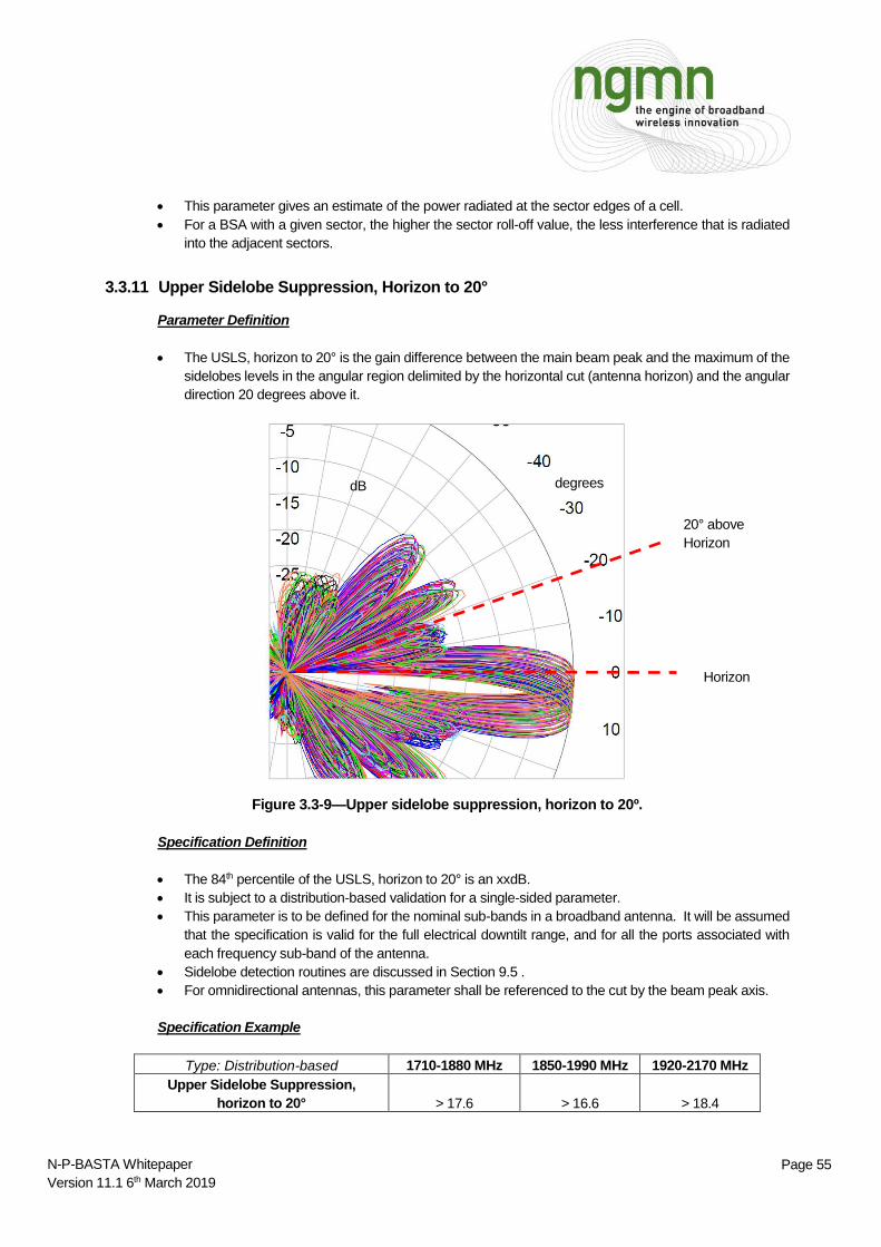
t
Page 55 N-P-BASTA Whitepaper
Version 11.1 6th March 2019
This parameter gives an estimate of the power radiated at the sector edges of a cell.
For a BSA with a given sector, the higher the sector roll-off value, the less interference that is radiated
into the adjacent sectors.
3.3.11 Upper Sidelobe Suppression, Horizon to 20°
Parameter Definition
The USLS, horizon to 20° is the gain difference between the main beam peak and the maximum of the
sidelobes levels in the angular region delimited by the horizontal cut (antenna horizon) and the angular
direction 20 degrees above it.
Figure 3.3-9—Upper sidelobe suppression, horizon to 20º.
Specification Definition
The 84th percentile of the USLS, horizon to 20° is an xxdB.
It is subject to a distribution-based validation for a single-sided parameter.
This parameter is to be defined for the nominal sub-bands in a broadband antenna. It will be assumed
that the specification is valid for the full electrical downtilt range, and for all the ports associated with
each frequency sub-band of the antenna.
Sidelobe detection routines are discussed in Section 9.5 .
For omnidirectional antennas, this parameter shall be referenced to the cut by the beam peak axis.
Specification Example
Type: Distribution-based 1710-1880 MHz 1850-1990 MHz 1920-2170 MHz
Upper Sidelobe Suppression,
horizon to 20° > 17.6 > 16.6 > 18.4
Horizon
20° above
Horizon
dB degrees

t
Page 56 N-P-BASTA Whitepaper
Version 11.1 6th March 2019
XML - Tag Example
<upper_sidelobe_suppression_horizon_to_20 value="18.4"/>
Relevance
This parameter indicates the amount of interfering signal radiated above the horizon due to the upper
sidelobes presence.
It also indicates the minimum suppression level of the sidelobes above the main beam in a 20° sector
above the horizon.
3.3.12 Maximum Upper Sidelobe Suppression
Parameter Definition
The maximum upper sidelobe suppression is in the elevation cut the gain difference between the main
beam peak and the highest level amidst all the sidelobes above the main beam peak and up to the
zenith.
Figure 3.3-10—Maximum Upper Sidelobe Suppression.
Specification Definition
The ratio of the main beam peak and any Upper SLS must be greater than value in xxdB in 84th
Percentile of the test samples
Angular region of specification -
main beam peak to zenith
Main beam peak example
10º electrical tilt
Degrees
dB
Elevation Pattern
Zenith
Maximum upper sidelobe

t
Page 57 N-P-BASTA Whitepaper
Version 11.1 6th March 2019
The angular region of specification elongates from the main beam peak to the zenith.
It is subject to a distribution-based validation for a single-sided parameter.
This parameter is to be defined for the nominal sub-bands in a broadband antenna. It will be assumed
that the specification is valid for the full electrical downtilt range, and for all the ports associated with
each frequency sub-band of the antenna.
For omnidirectional antennas, this parameter shall be referenced to the cut by the beam peak axis.
Specification Example
Type: Distribution-based 1710-1880 MHz 1850-1990 MHz 1920-2170 MHz
Maximum Upper Sidelobe Suppression > 14.3 > 15.1 > 15.6
XML - Tag Example
<maximum_upper_sidelobe_suppression value="14.3"/>
Relevance
Upper sidelobes are generally undesirable, considering that even if they do not create interference, they
represent energy radiated in unwanted directions and therefore lost to the system. Consequently a low
value of maximum upper sidelobe suppression is beneficial.
3.3.13 Azimuth Interference Ratio
Parameter Definition
AIR is defined as the ratio of the integrated radiation intensity inside the antenna’s sector edges to its
integrated interfering radiation. The sector is in this case referenced to the projection of the mechanical
boresight onto the azimuth pattern.
Specification Definition
It is subject to a distribution-based validation for a double-sided parameter.
The AIR is defined as the combination of a typical (mean) value and a tolerance, both in dB.
It is calculated from both the Co-pol pattern and the Cr-pol pattern in the form of:
AIR = 10*log((Pd/(Pu))
Where:
o Pd is defined as the integrated in sector radiation intensity calculated as the square root of sum of
copolar gain squared and x-polar gain squared, summed over all directions inside the sector.
o Pu is defined as the corresponding sum outside the sector
the angular resolution of the gain measurements must be the same in the entire
azimuth pattern

t
Page 58 N-P-BASTA Whitepaper
Version 11.1 6th March 2019
This parameter is to be defined for the nominal sub-bands in a broadband antenna. It will be assumed
that the specification is valid for the full electrical downtilt range, and for all the ports associated with
each frequency sub-band of the antenna.
For multi-beam antennas type II, this parameter shall not be given.
For omnidirectional antennas, this parameter shall not be given.
Specification Example
Type: Distribution-based 1710-1880 MHz 1850-1990 MHz 1920-2170 MHz
Azimuth Interference Ratio 11.0 ± 0.5 11.5 ± 0.6 11.8 ± 0.7
XML - Tag Example
<azimuth_interference_ratio value="11.0" tolerance="0.5"/>
Relevance
It is a parameter that allows comparison of various antennas’ rejection of interference to cells illuminated
from the same site.
3.3.14 Azimuth Beam Pan Angles
Parameter Definition
The azimuth beam pan angles are the nominal beam directions in the azimuth plane, which the antenna
can point to, when its beam is electrically steered.

t
Page 59 N-P-BASTA Whitepaper
Version 11.1 6th March 2019
Figure 3.3-11—Some patterns of an azimuth beam steering antenna (pan angles: -30°; 0°; +30°).
Specification Definition
It is a list of relevant pan angles with respect to the antenna mechanical boresight (pan = 0°).
The values in the list are nominal ones in degrees.
Negative values shall indicate counterclockwise beam panning, vice versa positive values shall indicate
clockwise beam panning.
Since electrical beam panning in the azimuth plane is conceptually similar to electrical tilting in the
elevation plane, the recommendations on the relevant pan angles are the same as those specified for
the electrical downtilt (see Section 4.2), except that the angular resolution shall in this case be at least
10 degrees. Pan = 0° shall be the reference for the all the other angles.
Since different pan angles produce different antenna patterns, the antenna’s parameters shall be
described for each pan angle by a single XML file (see Section 10.1), which shall be named
accordingly (see Section 10.1.1).
Specification Example
List of XML files of the same datasheet version of an antenna “XYZ” capable of steering between -30° and
+30°:
BASTA10-0_CELLMAX_XYZ,PANM030_1999-12-30_V00_F.xml
BASTA10-0_CELLMAX_XYZ,PANM020_1999-12-30_V00_F.xml
BASTA10-0_CELLMAX_XYZ,PANM010_1999-12-30_V00_F.xml
BASTA10-0_CELLMAX_XYZ,PANP000_1999-12-30_V00_F.xml
BASTA10-0_CELLMAX_XYZ,PANP010_1999-12-30_V00_F.xml
BASTA10-0_CELLMAX_XYZ,PANP020_1999-12-30_V00_F.xml
BASTA10-0_CELLMAX_XYZ,PANP030_1999-12-30_V00_F.xml
XML - Tag Example
Not applicable
Relevance
This is one of the parameters contributing to the characteristics and extent of the cell sector coverage.
It is a parameter that can be adjusted for:
o Sector alignment and hand-off optimization.
o RF coverage and interference optimization.
o Sector load balancing.
3.3.15 Azimuth Beamwidth Fan
Parameter Definition
For an electrically variable azimuth beamwidth antenna, the azimuth beamwidth fan is the list of nominal
azimuth half-power beamwidths that the antenna can be set to exhibit by electrically altering its beam.

t
Page 60 N-P-BASTA Whitepaper
Version 11.1 6th March 2019
Figure 3.3-12— Patterns of a variable azimuth beamwidth BSA (35°/65°/105° pattern overlays).
Specification Definition
For the purpose of this whitepaper, a fan angle is defined as the nominal H_HPBW (see Section 2.8)
of one of the possible azimuth patterns of an electrically variable azimuth beamwidth antenna.
It is a list of relevant fan angles.
The values in the list are nominal ones in degrees.
Since different fan angles produce different antenna patterns, the antenna’s parameters shall be
described for each fan angle by a single XML file (see Section 10.1), which shall be named accordingly
(see Section 10.1.1).
The parameters of antennas that are not able to vary their beam continuously shall be described by a
single XML file for each fan angle possibility.
The parameters of antennas that are able to vary their beam continuously shall be described by a single
XML file for each relevant fan angle. The recommendations on the relevant fan angles are similar to
those specified for the electrical downtilt (see Section 4.2), except that the angular resolution shall in
this case be at least 10 degrees. The lowest fan angle shall be the reference for the all the other ones.
Specification Example
List of XML files of the same datasheet version of an antenna “XYZ” capable of varying its H_HPBW only to
35°, 65° and 105°:
BASTA10-0_AMPHENOL_XYZ,FAN035_2007-05-01_V02_P.xml
BASTA10-0_AMPHENOL_XYZ,FAN065_2007-05-01_V02_P.xml
BASTA10-0_AMPHENOL_XYZ,FAN105_2007-05-01_V02_P.xml
List of XML files of the same datasheet version of an antenna “XYZ” capable of varying its H_HPBW
continuously between 65° and 90°:
BASTA10-0_AMPHENOL_XYZ,FAN065_2007-05-01_V02_P.xml

t
Page 61 N-P-BASTA Whitepaper
Version 11.1 6th March 2019
BASTA10-0_AMPHENOL_XYZ,FAN070_2007-05-01_V02_P.xml
BASTA10-0_AMPHENOL_XYZ,FAN080_2007-05-01_V02_P.xml
BASTA10-0_AMPHENOL_XYZ,FAN090_2007-05-01_V02_P.xml
XML - Tag Example
Not applicable
Relevance
This is one of the parameters contributing to the characteristics and extent of the cell sector coverage.
It is a parameter that can be adjusted for:
o Sector alignment and hand-off optimization.
o RF coverage and interference optimization.
o Sector load balancing.
3.3.16 Maximum Effective Power of Cluster
Parameter Definition
The maximum power, which can be transmitted into one antenna cluster, and which shall be withstood
by the antenna without it suffering permanent damage or being mechanically or electrically affected
(hence subject to parameters’ alteration).
Specification Definition
Power is defined as effective CW power.
This is an absolute, maximum parameter specified in Watts.
It is specified at sea level over the environmental conditions specified for the antenna.
Specification shall reference the full frequency range, full electrical downtilt range, and the associated
ports of the cluster.
Specification Example
Type: Absolute 1710-2170 MHz
Maximum Effective Power of Cluster 500
XML - Tag Example
<maximum_effective_power_cluster value="500"/>
Relevance
Exceeding the specified power rating can damage the antenna.

t
Page 62 N-P-BASTA Whitepaper
Version 11.1 6th March 2019
4 Validation and Specification of RF Parameters
4.1 Industry Practice for Base Station Antennas
In a commercial RFQ process cellular operators specify the expected performance of the antennas that
need to be purchased for deployment in their networks. Detailed specifications are provided to antenna
vendors, who respond with specification datasheets or other documentation that compares how the
performance of their products complies with the RFQ requirements. In order to accurately compare the
properties of one antenna vendor’s product with another’s, all parties in the supply chain shall have a
common understanding of the antenna parameters definitions, and just as critically, of the methodology used
to calculate and validate the associated specifications. This section of the whitepaper addresses the
calculation and validation of the RF specifications.
4.2 General Guidance
For the validation and the specification of radiation pattern derived parameters, the NGMN guidelines
require a specific set of sub-bands and associated frequencies to be measured and analyzed. See
Section 9.1 for details.
Parameters are classified as absolute or distribution-based. Distribution-based parameters are
further classified as single-sided parameters or double-sided parameters.
In general, absolute parameters are defined for the full frequency range of an antenna, and are based
on swept frequency measurements of the input ports. For these parameters, unless otherwise noted,
it will be assumed that the specification is valid for the full frequency range, full electrical downtilt range,
and all the associated ports of the antenna. E.g.: 1710-2170 MHz; 0°-10°; +45 and -45 ports.
In general, distribution-based parameters are defined in sub-bands of the full frequency range of an
antenna, and are based on radiation pattern measurements. For these parameters, unless otherwise
noted, it will be assumed that the specification is valid for the full sub-band frequency range, full electrical
downtilt range, and all associated ports of the antenna. E.g.: 1710-1880 MHz; 0°-10°; +45 and -45
ports.
Typical parameters are distribution-based parameters that are defined by a mean value and a
tolerance. If the specification’s measured values constituted a normal (Gaussian) probability
distribution, the tolerance would be defined as ± 1.5 standard deviations. The reason why these
parameters are also called double-sided lies in the fact that typical parameters are validated by a set
of measured data points revolving around the mean value, both to its “left side” (- tolerance) and to the
“right side” (+ tolerance) in the distribution function.
o Gain is a special case of a typical parameter. It is specified for each of the sub-bands included in
the frequency range of the antenna, for the associated ports and for the specific lowest, middle,
and highest tilt values over the electrical tilt range of the antenna. In addition, an “over all tilts” (all
the electrical tilt angles are included in the calculation) gain is specified as a standard typical
parameter.
Maximum or minimum parameters are distribution-based parameters that are defined by a threshold
value. If the specification’s measured values constituted a normal (Gaussian) probability distribution,
the maximum threshold value would be determined by their mean value plus one standard deviation,
while the minimum threshold value would be determined by their mean value minus one standard
deviation. The reason why these parameters are called single-sided lies in the fact that these
parameters are validated by a set of measured data points, respectively only to the “left side” (for
t
Page 63 N-P-BASTA Whitepaper
Version 11.1 6th March 2019
“maximum” parameters) or only to the “right side” (for “minimum” parameters) of a threshold in the
distribution function.
o Elevation downtilt deviation is a special case of a maximum parameter. The absolute maximum
differences between the real tilt values (calculated as specified in Section 3.2.6) and the nominal
tilt degree shall be calculated, and with those the parameter shall be specified for each of the sub-
bands included in the frequency range of the antenna, for the associated ports and for the whole
tilt range.
For the single-sided parameters that use decibels as measurement unit there shall be no more than 3
dB excursion beyond the specified value. For example, if the threshold for the first upper sidelobe
suppression was specified as 15.2 dB, there should be no value lower than 12.2 dB in the whole set of
measured values. If that happens, the parameter specified value shall be adjusted so that the excursion
is exactly 3 dB
Some parameters require the measurement of Co-Pol as well as Cr-Pol patterns, both of which
require a scrupulous alignment of the whole measurement system (see Figure 56). A misalignment
can lead to sub-optimal figures, due to the decrease of Co-Pol amplitudes and increase of the Cr-Pol
ones.
Pattern data shall be extracted at a minimum of 1° angular resolution if the pattern has an average
HPBW equal to 20° or broader. Vice versa if the pattern has an average HPBW of less than 20°, it can
happen that the patterns exhibit some “spikes”: under these circumstances, these sudden changes of
pattern level shall be handled by extracting pattern data with 0.5° angular resolution. This rule applies
only for the sake of parameters’ precision and shall not affect any other information that the vendors
provide to the operators (radio planning files, etc.).
Pattern data for antennas capable of electrical downtilt shall be taken with the same step at least every
1° over the entire specified tilt range. Antennas whose tilt-range starts and/or stops with half a degree
follow the same principle, except that if the chosen step is 1°, the first and/or last tilt shall be measured
with a step of 0.5° (e.g.: 2.5° to 10° downtilting antenna’s pattern data will be taken at: 2.5°; 3°; …; 10°.
2.5° to 10.5° downtilting antenna’s pattern data will be taken at: 2.5°; 3°; …; 10°; 10.5°.).
Pattern data shall be given for the elevation and azimuth pattern cuts.
Legacy vendor specification datasheets and legacy NGMN datasheets shall not be required to be
updated as a whole. It is foreseen that operators might request NGMN compliance for new RFQs and
new products, therefore the recommendations present in this document shall be only applied to
antennas that are developed after the date of its publication. Legacy NGMN datasheet shall therefore
keep their validity for legacy products.
4.3 Absolute RF Parameters
For absolute parameters, 100% of the measured data falls below a maximum value or above a minimum
value and distribution-based analysis is not necessary. In those cases there shall be no data points
excursions beyond the specified value.
Typically these parameters are specified for the full frequency range, full electrical downtilt range, and
associated ports of the antenna (for example: 1710-2170 MHz; 0°-10°; +45 and -45 ports).

t
Page 64 N-P-BASTA Whitepaper
Version 11.1 6th March 2019
4.4 Distribution-based RF Parameters
Considering that antennas’ patterns change with frequency, tilt and polarization, for certain parameters it is
not suitable to use absolute maxima or minima as metrics to evaluate an antenna’s performance. In fact,
by using them, a misrepresentation of the antenna could be likely. A very limited set of values (worst case:
a single one) amongst the entire dataset of measured ones would characterize a parameter, even though
all the other values are sensibly higher or lower. In these cases a distribution-based analysis excluding
worst and best values is necessary to give a better overview of the aforementioned performances.
4.4.1 General methodology
For a given antenna model, its radiation patterns are measured at the recommended frequencies (see
Section 9.1) for each of the required sub-bands in the full antenna bandwidth.
A full antenna bandwidth (or main frequency range) that is used only as an example in this section of the
whitepaper is: 1710-2170 MHz. The specified sub-bands that are used only as an example in this section
of the whitepaper are the following three:
Band 1710-2170 MHz
Sub-Bands 1710-1880 MHz 1850-1990 MHz 1920-2170 MHz
Recommendation on sub-bands can be found in Section 9.1.
For antennas with variable electrical downtilt, each individual pattern is measured (as specified in Section
4.2), analyzed, and finally a value is calculated according the definition of the chosen parameter. The
distribution of the resulting dataset of values is then analyzed, so that a single value that represents the
specification of that very parameter can be obtained.
In the table below it is shown an example of a full dataset of the azimuth beamwidth parameter for the sub-
band 1710-1880 MHz:
Table 4.4-1—Parameter dataset – single sub-band, all tilts, all ports.

t
Page 65 N-P-BASTA Whitepaper
Version 11.1 6th March 2019
4.4.2 Double-Sided Specifications
For some parameters, their relevance is best captured by how the whole calculated dataset revolves around
a typical value; therefore, these are designated as double-sided parameters (see also Section 4.2). Their
distribution-based validation is applied in the measurement units identified within their specification definition.
Figure 4.4-1—Double-sided specification for a normal distribution.
Even though the definition of double-sided parameters is inspired by Gaussian statistic, in reality most of the
parameters’ probability distribution are questionably a Gaussian curve. Even if the definition of mean (µ) is
obviously the same (it is the average of the values in the distribution as linear numbers), the tolerance
definitions do not coincide: for a normal distribution would simply be equal to ± 1.5 * standard deviation (σ);
for a real one instead, it is defined as the average of the distances from the mean of the two values,
both of which exclude from the distribution the 6.7% of the measured values, that is respectively its
far left side (from 0% to 6.7%) and its far right side (from 93.3% to 100%).
A normal distribution is also a continuous curve, but in the real world it is possible only to approximate a
probability distribution function using a sorted array of measured values (one value for each frequency,
polarization and tilt degree). Thus it is possible that the threshold values “mean - tolerance” (6.7th percentile)
and “mean + tolerance” (93.3rd percentile) are not values that were actually measured. Below it is shown a
block chart describing the algorithm to correctly find those:
Double-sided specification: 86.6% of the values “around the mean”
Mean - Tolerance
86.6%
Mean + Tolerance
Mean
6.7% 6.7%

t
Page 66 N-P-BASTA Whitepaper
Version 11.1 6th March 2019
Figure 4.4-2—Algorithm to find "mean - tolerance" and "mean + tolerance"
Once the two percentiles are found, the modulus of their differences from the mean value shall be averaged
in order to obtain a single number hence designated as tolerance.
4.4.3 Double-Sided Specification Example–Azimuth HPBW Validation
For this example of validation process, the calculation of the azimuth HPBW specification in the 1710-1880
MHz sub-band will be used.
First of all, the antennas radiation patterns for the sub-band are analyzed according to the parameter
definition (see Section 3.2.4):
Figure 4.4-3—Azimuth beam-peak patterns plots - 1710-1880 MHz, all ports, and all tilts.
Degrees
dB

t
Page 67 N-P-BASTA Whitepaper
Version 11.1 6th March 2019
The values for azimuth beamwidth are calculated for each frequency in the sub-band, each port, and each
downtilt setting:
Table 4.4-2—Complete dataset of azimuth HPBWs.
The distribution of the set of measured values is finally analyzed to determine the specification:
The array containing all the values above counts 126 elements (9 frequencies x 7 tilts x 2 polarizations).
The minimum value is 58.8° and the maximum is 70.8°. The mean is the sum of all the elements
(degrees do not need the conversion in linear numbers), divided by 126.
The proportion (126 – 1) : 100 = (x – 1) : 6.7 solved by x, returns x = 9.4. Where x is the array index of
the 6.7th percentile.
The proportion (126 – 1) : 100 = (x – 1) : 93.3 solved by x, returns x = 117.6. Where x is the array index
of the 93.3rd percentile.
Once the array is sorted in ascending fashion, it can be seen that the 9th element (index = 9) is 61.1°,
the 10th is 61.8, the 117th and 118th are both 69.4°.
Clearly, the “mean + tolerance” value is 69.4°, while for the “mean – tolerance” a linear interpolation
between 61.1° and 61.8° is necessary.
Using the following equivalences: z+ = 61.8°; z- = 61.1°; x+ = 10; x- = 9; the value of “mean - tolerance”
can be obtained: (z+-z) = 61.4°.
The modulus of the differences of the two values from the mean is respectively: 3.7° and 4.3°, therefore
the tolerance is their average, which is 4.0°.
Azimuth beamwidth # Array elements Min Max Mean Tolerance
1710-1880 MHz 126 58.8° 70.8° 65.1° 4.0°
Table 4.4-3—Summary of azimuth HPBW statistics.
The specification is set as:
Type: Distribution-based 1710-1880 MHz
Azimuth HPBW 65.1 ± 4.0
As previously stated, in this example, the azimuth HPBW has only been calculated for one sub-band (1710-
1880 MHz).
This procedure has to be repeated two additional times to populate the full specification table for the
parameter:
Type: Distribution-based 1710-1880 MHz 1850-1990 MHz 1920-2170 MHz
Azimuth HPBW 65.1 ± 4.0 64.8 ± 1.6 63.4 ± 2.3

t
Page 68 N-P-BASTA Whitepaper
Version 11.1 6th March 2019
For the purpose of this whitepaper, it is instructive to show the plotted the azimuth HPBW values as a
function of frequency, and the distribution of the calculated values in a histogram. These plots are shown
below:
Figure 4.4-4—Azimuth HPBW for each tilt and port as a function of the frequency.
Figure 4.4-5—Histogram of azimuth HPBW values.
The histogram above shows well that the distribution of the values is not Gaussian. In fact if the tolerance
would have been incorrectly calculated as 1.5 * σ, it would have been equal to 4.3°.
55 °
57 °
59 °
61 °
63 °
65 °
67 °
69 °
71 °
73 °
75 °
1710 MHz 1733 MHz 1748 MHz 1755 MHz 1785 MHz 1805 MHz 1843 MHz 1850 MHz 1880 MHz
H_H
PB
W
Frequency
0
0,02
0,04
0,06
0,08
0,1
0,12
0,14
0,16
0,18
0,2
58
,0 °
58
,5 °
59
,0 °
59
,5 °
60
,0 °
60
,5 °
61
,0 °
61
,5 °
62
,0 °
62
,5 °
63
,0 °
63
,5 °
64
,0 °
64
,5 °
65
,0 °
65
,5 °
66
,0 °
66
,5 °
67
,0 °
67
,5 °
68
,0 °
68
,5 °
69
,0 °
69
,5 °
70
,0 °
70
,5 °
Pro
bab
ility
Degrees

t
Page 69 N-P-BASTA Whitepaper
Version 11.1 6th March 2019
4.4.4 Single-sided Specifications
For some parameters, their relevance is best captured by how the dataset of calculated values fall above or
below a threshold value; therefore, they are designated as single-sided parameters (see also Section 4.2).
The distribution-based validation is applied in the units identified within the specification definition.
A “maximum” specification for a parameter is defined when the above mentioned dataset is mostly “below”
a specified value: this does not strictly mean that the values must be lower than it, since the physical meaning
of the parameter and its associated sign play an important role in the meaning of “below”.
For Gaussian statistics, the “maximum” would be a threshold value defined by the mean plus the standard
deviation, both calculated on the dataset used to validate the specification. Since µ+σ serves as limit for the
lower 84% of the values in a normal probability distribution, and since in reality the parameters’ distributions
are hardly Gaussian, a “maximum” will be generally defined as the value that demarcate the lower 84% of
the entire dataset. In other words, 84% of the measured values will fall below the given specification
(threshold).
Figure 4.4-6—Single-sided specification (maximum).
A “minimum” specification for a parameter is defined when the above mentioned dataset is mostly “above”
a specified value: this does not strictly mean that the values must be higher than it, since the physical
meaning of the parameter and its associated sign play an important role in the meaning of “above”.
For Gaussian statistics, the “minimum” would be a threshold value defined by the mean minus the standard
deviation, both calculated on the dataset used to validate the specification. Since µ-σ serves as limit for the
higher 84% of the values in a normal probability distribution, and since in reality the parameters’ distributions
are hardly Gaussian, a “minimum” will be generally defined as the value that demarcate the higher 84% of
the entire dataset. In other words, 84% of the measured values will fall above the given specification
(threshold).
“Maximum (<)” Specification: 84% of the values below a threshold
84% 16%
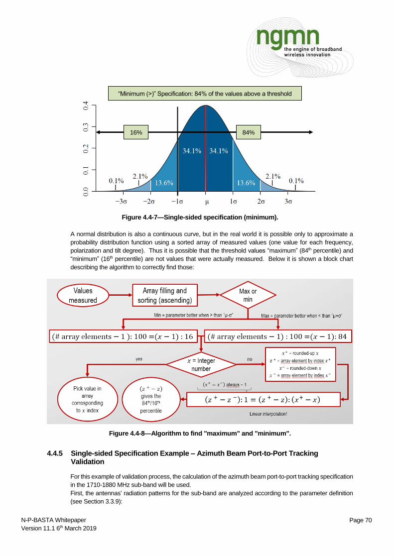
t
Page 70 N-P-BASTA Whitepaper
Version 11.1 6th March 2019
Figure 4.4-7—Single-sided specification (minimum).
A normal distribution is also a continuous curve, but in the real world it is possible only to approximate a
probability distribution function using a sorted array of measured values (one value for each frequency,
polarization and tilt degree). Thus it is possible that the threshold values “maximum” (84th percentile) and
“minimum” (16th percentile) are not values that were actually measured. Below it is shown a block chart
describing the algorithm to correctly find those:
Figure 4.4-8—Algorithm to find "maximum" and "minimum".
4.4.5 Single-sided Specification Example – Azimuth Beam Port-to-Port Tracking Validation
For this example of validation process, the calculation of the azimuth beam port-to-port tracking specification
in the 1710-1880 MHz sub-band will be used.
First, the antennas’ radiation patterns for the sub-band are analyzed according to the parameter definition
(see Section 3.3.9):
“Minimum (>)” Specification: 84% of the values above a threshold
84% 16%

t
Page 71 N-P-BASTA Whitepaper
Version 11.1 6th March 2019
Figure 4.4-9—Polarizations pattern level difference of a 90° sector antenna for one frequency and a
single downtilt degree.
Table 4.4-4—Complete dataset azimuth beam port-to-port tracking.
The distribution of the set of measured values is finally analyzed to determine the specification:
The array containing all the values in the table above counts 162 elements (9 frequencies x 9 tilts x 2
directions).
The minimum value is 0 dB and the maximum is 3.6 dB. The mean is the sum of all the elements (as
linear numbers) divided by 162.
In the table above the higher the number, the worse the signal difference, the worse the antenna’s
performance. To define the parameter 16% of the worst cases (higher values) are ruled out.
The proportion (162 – 1) : 100 = (x – 1) : 84 solved by x, returns x = 136.24. Where x is the array index
of the 84th percentile.
Since 136.24 is not an integer number, an interpolation is necessary.
Once the array is sorted in ascending fashion, it can be seen that the value lies between the 136th
element (index = 136), which is 2.7 dB, and the 137th element (index = 137) of the array, which is 2.8
dB.
The interpolation formula becomes: 0.1 : 1 = (2.8 – z) : (137-136.24) and ultimately gives a result of 2.7
dB.
Azimuth Beam Port-to-Port
Tracking # Array
elements Min = Best Max = Worst 84%
1710-1880 MHz 162 0 dB 3.6 dB 2.7 dB
Table 4.4-5—Summary of azimuth beam port-to-port tracking statistics.
The specification is set as:

t
Page 72 N-P-BASTA Whitepaper
Version 11.1 6th March 2019
Type: Distribution-based 1710-1880 MHz
Azimuth Beam Port-to-Port Tracking < 2.7
Note that the specification values are never more than 3 dB higher than the maximum found through the
algorithm.
As previously state, in this example, azimuth beam port-to-port tracking has only been calculated for one
sub-band (1710-1880 MHz).
This procedure has to be repeated two additional times to populate the full specification table for the azimuth
beam port-to-port tracking parameter:
Type: Distribution-based 1710-1880 MHz 1850-1990 MHz 1920-2170 MHz
Azimuth Beam Port-to-Port Tracking < 2.7 < 1.8 < 2.2
For the purpose of this whitepaper, it is instructive to show the plotted azimuth beam port-to-port tracking
values as a function of frequency, and the distribution of the calculated values in a histogram. These plots
are shown below:
Figure 4.4-10—Azimuth beam port-to-port tracking for each tilt and port as a function of the
frequency.
0,0 dB
0,5 dB
1,0 dB
1,5 dB
2,0 dB
2,5 dB
3,0 dB
3,5 dB
4,0 dB
1710 MHz 1733 MHz 1748 MHz 1755 MHz 1785 MHz 1805 MHz 1843 MHz 1850 MHz 1880 MHz
Azi
mu
th b
eam
po
rt-t
o-p
ort
tra
ckin
g
Frequency

t
Page 73 N-P-BASTA Whitepaper
Version 11.1 6th March 2019
Figure 4.4-11—Histogram azimuth beam port-to-port tracking.
The histogram above shows well that the distribution of the values is not Gaussian. In fact if the parameter
would have been incorrectly calculated as µ+σ, it would have been equal to 2.5 dB.
4.4.6 Single-sided Specification Example – Upper Sidelobe Suppression, Peak to 20° Validation
For this example of validation process, the calculation of the upper sidelobe suppression, peak to 20°
specification in the 1710-1880 MHz sub-band will be used.
First, the antennas’ radiation patterns for the sub-band are analyzed according to the parameter definition
(see Section 3.2.15):
0
0,02
0,04
0,06
0,08
0,1
0,12
0,14
0,16
0,18
0,2
0,22
0,24
0,0dB
0,2dB
0,4dB
0,6dB
0,8dB
1,0dB
1,2dB
1,4dB
1,6dB
1,8dB
2,0dB
2,2dB
2,4dB
2,6dB
2,8dB
3,0dB
3,2dB
3,4dB
3,6dB
Pro
bab
ility
dB

t
Page 74 N-P-BASTA Whitepaper
Version 11.1 6th March 2019
Figure 4.4-12—Worst sidelobe peak 20° above the main beam peak for one frequency, a single port
and a single downtilt degree.
Table 4.4-6—Complete dataset upper sidelobe suppression, peak to 20°.
The distribution of the set of measured values is finally analyzed to determine the specification:
The array containing all the values in the table above counts 126 elements (9 frequencies x 7 tilts x 2
polarizations).
The minimum value is 14.9 dB and the maximum is 19.8 dB. The mean is the sum of all the elements
(as linear numbers) divided by 126.
In the table above the higher the number, the smaller the sidelobe, the better the antenna’s
performance. To define the parameter 16% of the worst cases (lower values) are ruled out.
The proportion (126 – 1) : 100 = (x – 1) : 16 solved by x, returns x = 21. Where x is the array index of
the 16th percentile.
Since 21 is an integer number, no interpolation is necessary.
Once the array is sorted in ascending fashion, it can be seen that the 21st element (index = 21) is 15.8
dB.
Upper sidelobe suppression,
peak to 20° # Array
elements Min = Worst Max = Best 16%
1710-1880 MHz 126 14.9 dB 19.8 dB 15.8 dB
Table 7—Summary of upper sidelobe suppression, peak to 20° statistics.
The specification is set as:
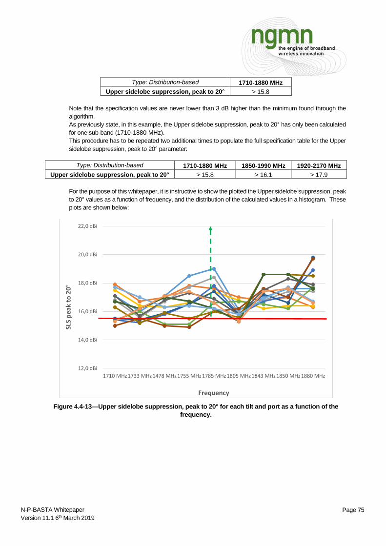
t
Page 75 N-P-BASTA Whitepaper
Version 11.1 6th March 2019
Type: Distribution-based 1710-1880 MHz
Upper sidelobe suppression, peak to 20° > 15.8
Note that the specification values are never lower than 3 dB higher than the minimum found through the
algorithm.
As previously state, in this example, the Upper sidelobe suppression, peak to 20° has only been calculated
for one sub-band (1710-1880 MHz).
This procedure has to be repeated two additional times to populate the full specification table for the Upper
sidelobe suppression, peak to 20° parameter:
Type: Distribution-based 1710-1880 MHz 1850-1990 MHz 1920-2170 MHz
Upper sidelobe suppression, peak to 20° > 15.8 > 16.1 > 17.9
For the purpose of this whitepaper, it is instructive to show the plotted the Upper sidelobe suppression, peak
to 20° values as a function of frequency, and the distribution of the calculated values in a histogram. These
plots are shown below:
Figure 4.4-13—Upper sidelobe suppression, peak to 20° for each tilt and port as a function of the
frequency.
12,0 dBi
14,0 dBi
16,0 dBi
18,0 dBi
20,0 dBi
22,0 dBi
1710 MHz1733 MHz1478 MHz1755 MHz1785 MHz 1805 MHz1843 MHz 1850 MHz1880 MHz
SLS
pea
k to
20
°
Frequency

t
Page 76 N-P-BASTA Whitepaper
Version 11.1 6th March 2019
Figure 4.4-14—Histogram Upper sidelobe suppression, peak to 20°.
The histogram above shows well that the distribution of the values is not Gaussian. If the parameter would
have been incorrectly calculated as µ-σ, it would have been equal to 15.7 dB.
4.5 Sidelobe Suppression Calculation and Validation
The calculation of all the parameters related to the sidelobes (in this paper: “first sidelobe suppression”, “null
fill”, “upper sidelobe suppression, peak to 20°” and “upper sidelobe suppression, horizon to 20°”) is only
apparently uncomplicated, due to the fact that not all the sidelobes’ peaks are displayed as relative maxima
in the elevation pattern. It is in fact possible that some of them (especially the first sidelobe above and/or
below the main beam) are “merged” to another one (rare) or to the main beam (common). Should this
eventuality occur, the sidelobe peak would at best be visible as an inflection point, but it could alternatively
not be visible at all.
0,0
0,1
0,1
0,2
0,2
0,3
14,0 dB14,5 dB15,0 dB15,5 dB16,0 dB16,5 dB17,0 dB17,5 dB18,0 dB18,5 dB19,0 dB19,5 dB20,0 dB
Pro
bab
ility
dB

t
Page 77 N-P-BASTA Whitepaper
Version 11.1 6th March 2019
Figure 4.5-1—First upper sidelobe merged into main beam.
It is necessary to address this issue from the perspective of an automated calculation process, rather than
relying on a visual analysis of the elevation pattern. On this wise some algorithms for the correct calculation
of the above mentioned parameters will be described in the forthcoming sections.
4.5.1 First Sidelobe Suppression
Several empirical tests were conducted amongst a number of antennas with different performances and
characteristics, and those suggested that the first sidelobe above (counterclockwise in the elevation pattern)
the main beam commonly appeared as a relative maximum in a sector equal to the V_HPBW multiplied by
1.78 above the main beam peak. For all the remaining cases where the elevation pattern did not exhibit
any relative maximum in that sector, the tests showed a very high probability that the peak of a merged
sidelobe could be found by, or immediately in proximity to, the angular direction corresponding to V_HPBW
* 1.55 degrees above the main beam peak.
Consequently, the first sidelobe peak shall be determined by executing the following steps for each
frequency, tilt and polarization involved in the calculation:
Locate main beam’s maximum in the elevation pattern.
Locate the first relative minimum above main beam’s maximum.
Locate the first relative maximum above the first relative minimum.
Calculate the V_HPBW.
If the angular position of the first relative maximum lies in the range delimited by the main beam peak
and the angular direction represented by 1.78 * V_HPBW degrees above it, then the corresponding
pattern level shall be selected as the peak of the first sidelobe above the main beam peak.
If the angular position of the first relative maximum lies above the sector defined in the previous point,
then the pattern level corresponding to the angular position marked by 1.55 * V_HPBW degrees above
the main beam peak shall represent the level of the (merged) first sidelobe above the main beam peak.
No relative maximum.
“Merged sidelobe”
clearly visible.
t
Page 78 N-P-BASTA Whitepaper
Version 11.1 6th March 2019
Note: The above mentioned tests were conducted using a resolution of 0.5° in the
elevation pattern, and with a set of antennas, whose V_HPBW never exceeded a broadness of 20
degrees.
4.5.2 Null fill
According to the definition in Section 3.3.3, the null fill parameter estimates the pattern level of the first
relative minimum below (clockwise in the elevation pattern) the main beam. Comparably to what happens
for the first sidelobe suppression (see previous section), it is possible that merged sidelobes show up in the
section of the elevation pattern situated below the main beam peak. In this case the first null does not
appear as a relative minimum, but coincides with the peak of the merged sidelobe, as its angular position
matches the end of the main beam. The aforementioned tests within the same conditions (see previous
section and the note at its foot), have proven to be valid for the first sidelobe below the main beam peak too,
consequently the steps to execute in order to determine the null fill are the following ones:
Locate main beam’s maximum in the elevation pattern.
Locate the first relative minimum below main beam’s maximum.
Locate the first relative maximum above the first relative minimum.
Calculate the V_HPBW.
If the angular position of the first relative maximum lies in the range delimited by the main beam peak
and the angular direction represented by 1.78 * V_HPBW degrees below it, then the corresponding
pattern level shall represent the peak of the first sidelobe below the main beam peak. In this case the
null fill shall correspond to the relative minimum found before (second point of this list).
If the angular position of the first relative maximum lies outside the sector defined in the previous point,
then the beam level corresponding to the angular position marked by 1.55 * V_HPBW degrees below
the main beam peak shall represent the level of the (merged) first sidelobe below the main beam peak.
The null fill shall have, in this case, the same value of the peak of the first sidelobe below the main beam
peak.
4.5.3 Upper Sidelobe Suppression, Peak to 20° / Horizon to 20°
As stated in Section 3.2.15 and Section 3.3.12, the “upper sidelobe suppression, peak to 20°” and the “upper
sidelobe suppression, horizon to 20°” estimate the worst level of a sidelobe inside their appropriate sectors
defined in the elevation pattern.
Yet, especially for antenna beams that have a very broad V_HPBW (e.g.: mechanically short antennas at
low frequencies), it can happen that there is no sidelobe peak in the sector delimited by the main beam peak
and 20 degrees above (counterclockwise in the elevation pattern) it or by the horizon and 20 degrees above
(counterclockwise in the elevation pattern) it.
In these cases, only one of the following three circumstances can occur:
In the analyzed sector there is only the first merged sidelobe peak.
In the analyzed sector there is only a portion of a sidelobe.
In the analyzed sector there only the main beam is contained.
For each of these circumstances there is an appropriate method to calculate the correct value for the
parameter to evaluate. Respectively:
The first merged sidelobe peak is treated as any other sidelobe peak. Since it does lie in the sector
under observation, the specification of the studied parameter shall be in fact equal to the first merged
sidelobe peak value.

t
Page 79 N-P-BASTA Whitepaper
Version 11.1 6th March 2019
The specification of the studied parameter shall be equal to the highest level of the portion of the
sidelobe included in the sector under observation.
The specification of the studied parameter shall be temporarily set to “not available”.
A deeper analysis is required in case one or more measurement points appear as “not available”. After
having calculated the specification for all the measurement points (one for each combination of frequency,
tilt and polarization), it is necessary to determine the quantity of “not available” data in respect to the one
that has been associated to a numeric value instead. If the “not available” are more than 50% of the whole
dataset, then the distribution-based evaluation of the parameter is skipped, and its specification shall be
instead set to “not applicable”. On the contrary, if there are at least 50% of numeric values in the above
mentioned dataset, then all the “not available” shall be substituted by 22 dB and the distribution-based
evaluation of the parameter is performed as usual.
The value of 22 dB has been selected after a research on the “upper sidelobe
suppression, peak to 20°” and “upper sidelobe suppression, horizon to 20°” specifications. This
value appeared to be the one most of the measurement points lean to. It has also been proven, that
the substitutions of 22 dB to the “not applicable” don’t polarize much the single-sided distribution-
based evaluation of the above mentioned parameters, which means that this value lets the
performance of the antenna remain accurate enough.
4.6 Gain Validation
Gain values are typically determined by the “gain by substitution” method, or the “gain by directivity / loss”
method (see Section 9.3 for their description). Both can be used to validate the specification of the gain,
and the validation process described below is applicable to the dataset of the parameter generated by either
method.
The gain specification is based on the values measured on all relevant ports, over the specified sub-band
frequency ranges, and at the low, mid, and high electrical downtilt settings. A “gain over all tilts” is also
specified, and it is calculated using measurements over all the antenna electrical downtilt values. In other
words, gain is to be specified in two ways:
At the specific minimum, middle, and maximum values of an antenna’s tilt range. In this case, the
validation data for each specified tilt is analyzed only at that tilt, not within a range of tilt degrees.
Over all tilts of an antenna’s tilt range. In this case, the validation data is analyzed over the entire tilt
range as measured in specific increments of electrical downtilt (see Section 4.2).
Gain measurements shall be carried out carefully to ensure their certainty. They can be difficult to be
precisely repeated, because the accuracy and repeatability of those measurements is determined by a
number of factors (this is better described in Section 9.4). Industry experts outline the discrepancy between
gain measurements as a number that oscillates between 0.5 dB and 1.0 dB. The repeatability margin
specification recommended for gain in this whitepaper is 0.8 dB, which is a value based on the experience
of the above mentioned experts, and is applied to all the antennas covered by this document, measured on
all calibrated antenna ranges, at any time, in good environmental conditions.
4.6.1 Gain Validation for a Single Tilt Value
For this example of validation process, the calculation of the gain specification in the 1710-1880 MHz sub-
band and by 0 degrees of electrical tilt will be used.

t
Page 80 N-P-BASTA Whitepaper
Version 11.1 6th March 2019
Gain Type: Distribution-based 1710-1880 MHz 1850-1990 MHz 1920-2170 MHz
0 Tilt 17.1 17.4 17.7
5 Tilt 17.3 17.5 17.7
10 Tilt 17.0 17.0 17.2
First of all, the antennas radiation patterns for the sub-band are analyzed according to the parameter
definition (see Section 3.2.3). The values for gain are measured for each frequency in the sub-band, each
port, and 0 degrees of electrical downtilt:
Table 4.6-1—Complete dataset for gain (1710-1880 MHz, 0° tilt).
The distribution of the set of measured values is finally analyzed to determine the specification (in this case
the mean, which shall be calculated over the magnitude and then reconverted in dBi):
Total Gain, dBi Min Max Mean
1710-1880 MHz 16.9 17.4 17.1
Table 4.6-2—Summary of gain statistics (1710 – 1880 MHz, 0° tilt).
The specification is finally set to 17.1 dBi.
As previously state, in this example, the gain has only been calculated for one sub-band (1710-1880 MHz).
This procedure has to be repeated two additional times to populate the full specification table for the gain
parameter by 0 degrees of electrical downtilt:
Type: Distribution-based All ports 1710-1880 MHz 1850-1990 MHz 1920-2170 MHz Gain 0 Tilt 17.1 17.4 17.7
The same has to be done for the other two tilts (middle and maximum, being 0° the minimum):
Type: Distribution-based All ports 1710-1880 MHz 1850-1990 MHz 1920-2170 MHz
Gain
0 Tilt 17.1 17.4 17.7
5 Tilt 17.3 17.5 17.7
10 Tilt 17.0 17.0 17.2
Per this whitepaper’s guidelines, the repeatability margin associated with a 17.1 dBi gain specification is
17.1 dBi – 0.8 dBi, or 16.3 dBi.
For the purpose of this whitepaper, it is instructive to show the plotted the gain values as a function of
frequency, the distribution of the calculated values in a histogram, and the gain with its repeatability margin.
These plots are shown below:

t
Page 81 N-P-BASTA Whitepaper
Version 11.1 6th March 2019
Figure 4.6-1—Gain plot for 0º tilt, both ports.
Figure 4.6-2—Gain histogram.
17.1 dBi

t
Page 82 N-P-BASTA Whitepaper
Version 11.1 6th March 2019
Figure 4.6-3—Gain plot with repeatability margin.
4.6.2 Gain Over All Tilts Validation
In this specification the gain is averaged for all values of the tilt range (see Section 4.2 for an explanation of
“all values of the tilt range”). For this example of validation process, the calculation of the “gain over all tilts”
specification in the 1850-1990 MHz sub-band will be used.
First of all, the antennas radiation patterns for the sub-band are analyzed according to the parameter
definition (see Section 3.2.3). The values for gain are measured for each frequency in the sub-band, each
port, and the whole range of electrical downtilt.
Table 4.6-3—Complete dataset of gain.
The distribution of the set of measured values is finally analyzed to determine the specification:
The array containing all the values above counts 198 elements (9 frequencies x 11 tilts x 2
polarizations).
The minimum value is 16.9 dBi and the maximum is 17.9 dBi. The mean is the sum of all the elements
in magnitude divided by 198 and then reconverted in dB.
The proportion (198 – 1) : 100 = (x – 1) : 6.7 solved by x, returns x = 14.2. Where x is the array index
of the 6.7th percentile.
0.8 dB repeatability
17.1 dBi
16.3 dBi

t
Page 83 N-P-BASTA Whitepaper
Version 11.1 6th March 2019
The proportion (198 – 1) : 100 = (x – 1) : 93.3 solved by x, returns x = 184.8. Where x is the array index
of the 93.3rd percentile.
Once the array is sorted in ascending fashion, it can be seen that the 14th (index = 14) and 15th elements
are both is 17.1 dBi, while the 184th and 185th are both 17.8 dBi.
Clearly, the “mean + tolerance” value is 17.8 dBi, while “mean - tolerance” value is 17.1 dBi.
The modulus of the differences of the two values from the mean is respectively: 0.3 dB and 0.4 dB,
therefore the tolerance is their average, which is 0.3 dB.
Gain over all tilts # Array elements Min Max Mean Tolerance
1850-1990 MHz 198 16.9 dBi 17.9 dBi 17.5 dBi 0.3 dBi
Table 4.6-4—Summary of gain statistics, over all tilts, 1850-1990 MHz.
The specification is set by the rounding of the mean value to 17.5 dBi and the rounding of the tolerance to
0.3 dB:
Type: Distribution-based All ports 1850-1990 MHz Gain Over all tilts 17.5 dBi ± 0.3 dB
As previously state, in this example, the gain over all tilts has only been calculated for one sub-band (1850-
1990 MHz).
This procedure has to be repeated two additional times to populate the full specification table for the
parameter:
Type: Distribution-based All ports 1710-1880 MHz 1850-1990 MHz 1920-2170 MHz Gain Over all tilts 17.4 ± 0.2 17.5 ± 0.3 17.9 ± 0.3
Below a table of the whole gain specification:
Type: Distribution-based All ports 1710-1880 MHz 1850-1990 MHz 1920-2170 MHz
Gain
0 Tilt 17.1 17.4 17.7
5 Tilt 17.3 17.5 17.7
10 Tilt 17.0 17.0 17.2
Over all tilts 17.4 ± 0.2 17.5 ± 0.3 17.9 ± 0.3
For the purpose of this whitepaper, it is instructive to show the plotted gain over all tilts values as a function
of frequency, and the distribution of the calculated values in a histogram. These plots are shown below:

t
Page 84 N-P-BASTA Whitepaper
Version 11.1 6th March 2019
Figure 4.6-4—Gain for each tilt and port as a function of the frequency.
Figure 4.6-5—Gain histogram.
The repeatability margin value of 0.8 dBi is graphed below:
16,5 dBi
17,0 dBi
17,5 dBi
18,0 dBi
1850MHz
1880MHz
1910MHz
1920MHz
1930MHz
1950MHz
1960MHz
1980MHz
1990MHz
Gai
n o
ver
all t
ilts
Frequency
0,00
0,05
0,10
0,15
0,20
0,25
0,30
0,35
0,40
16,0 dBi 16,2 dBi 16,4 dBi 16,6 dBi 16,8 dBi 17,0 dBi 17,2 dBi 17,4 dBi 17,6 dBi 17,8 dBi 18,0 dBi
Pro
bab
ility
dBi

t
Page 85 N-P-BASTA Whitepaper
Version 11.1 6th March 2019
Figure 4.6-6—Gain plot with repeatability margin.
The histogram above shows well that the distribution of the values is not Gaussian, even if the tolerance
incorrectly calculated as 1.5 * σ would have had the same value of 0.3 dB.
4.7 Validation of Elevation Downtilt Deviation
For this example of the validation process, the calculation of the elevation downtilt deviation specification in
the antenna sub-bands of 1710-1880 MHz, 1850-1990 MHz, and 1920-2170 MHz will be used.
First of all, the antennas radiation patterns for the sub-bands are analyzed according to the parameter
definition (see Section 3.2.7). The values for the real electrical downtilt are measured (see Section 3.2.6)
for each frequency in the sub-band, each port, and the whole range of electrical downtilt.
16,5 dBi
17,0 dBi
17,5 dBi
18,0 dBi
1850MHz
1880MHz
1910MHz
1920MHz
1930MHz
1950MHz
1960MHz
1980MHz
1990MHz
Gai
n o
ver
all t
ilts
Frequency
17.5 dBi
16.7 dBi
0.8 dBi repeatability
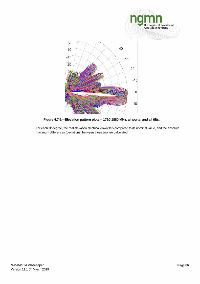
t
Page 86 N-P-BASTA Whitepaper
Version 11.1 6th March 2019
Figure 4.7-1—Elevation pattern plots – 1710-1880 MHz, all ports, and all tilts.
For each tilt degree, the real elevation electrical downtilt is compared to its nominal value, and the absolute
maximum differences (deviations) between those two are calculated:
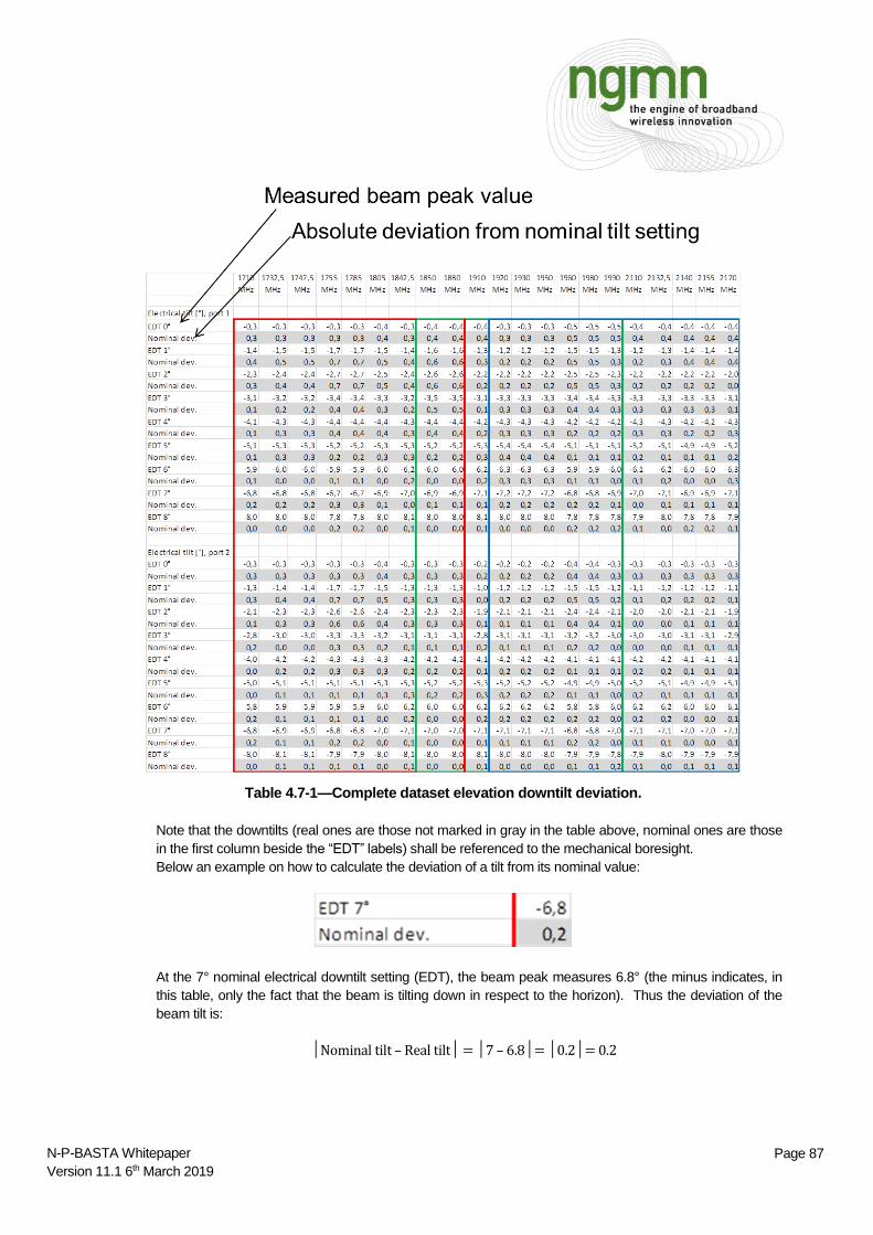
t
Page 87 N-P-BASTA Whitepaper
Version 11.1 6th March 2019
Table 4.7-1—Complete dataset elevation downtilt deviation.
Note that the downtilts (real ones are those not marked in gray in the table above, nominal ones are those
in the first column beside the “EDT” labels) shall be referenced to the mechanical boresight.
Below an example on how to calculate the deviation of a tilt from its nominal value:
At the 7° nominal electrical downtilt setting (EDT), the beam peak measures 6.8° (the minus indicates, in
this table, only the fact that the beam is tilting down in respect to the horizon). Thus the deviation of the
beam tilt is:
│Nominal tilt – Real tilt│ = │7 – 6.8│= │0.2│= 0.2

t
Page 88 N-P-BASTA Whitepaper
Version 11.1 6th March 2019
Once the complete dataset of deviations is obtained, the distribution of the parameter is analyzed to calculate
the specification. This is done no differently than the example in Section 4.4.6 for single-sided maximum
parameters.
Type: Distribution-based 1710-1880 MHz 1850-1990 MHz 1920-2170 MHz
Elevation Downtilt Deviation < 0.5 < 0.4 < 0.4
4.8 Guidance on Specifications Provided in Radio Planning Files
RF planning tool data file formats shall follow the same frequency and downtilt recommendations illustrated
in this document, preferably to the recommended frequencies specified in Section 9.1.3. The gain
parameter present in each pattern’s data file shall be equal to the actual measured gain determined when
the pattern was taken. Note that this procedure is different from what already specified for the gain
parameter.
5 Mechanical Parameters and Specifications
In this paper the mechanical parameters and the environmental specifications will always be, when not
specifically otherwise written, intended as required.
The format used for the mechanical parameters will be the same used for electrical specifications.
5.1 Antenna Dimensions
Parameter Definition
The outer antenna dimensions without additional antenna system components (e.g.: the mount or the
RET unit).
The dimensions are defined along the three axis of a Cartesian coordinate system defining the height
(H), the width (W) and the depth (D) of the product (see figure 5.1-1).
Specification Definition
The antenna dimensions are its nominal values specified in millimeters.
Height is measured along the vertical direction of the antenna in its intended mounting position (typically
this is also the largest dimension).
Width is measured along the horizontal direction of the antenna.
Depth is measured perpendicular to the plane spanned by vertical and horizontal direction.
The antenna RET installation reference plane is described by the H, W, or D dimension, but is actually
the plane normal (or most normal) to it.
Specification Example
Antenna without RET support:
o H x W x D: 1391mm x 183mm x 118mm.
o A RET actuator cannot be attached to the antenna.
Antenna with RET support:
o H x W x D: 1391mm x 183mm x 118mm.
o A RET actuator interface is present on the bottom of the antenna along the plane normal to its
height.
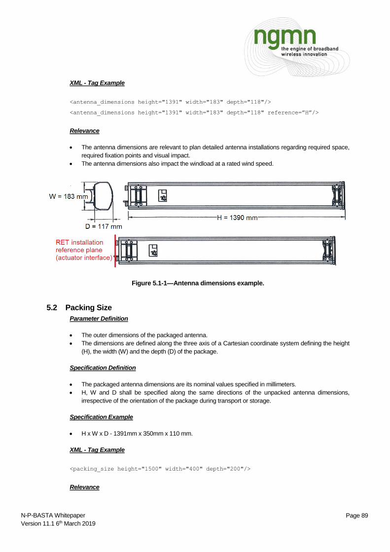
t
Page 89 N-P-BASTA Whitepaper
Version 11.1 6th March 2019
XML - Tag Example
<antenna_dimensions height="1391" width="183" depth="118"/>
<antenna_dimensions height="1391" width="183" depth="118" reference=”H”/>
Relevance
The antenna dimensions are relevant to plan detailed antenna installations regarding required space,
required fixation points and visual impact.
The antenna dimensions also impact the windload at a rated wind speed.
Figure 5.1-1—Antenna dimensions example.
5.2 Packing Size
Parameter Definition
The outer dimensions of the packaged antenna.
The dimensions are defined along the three axis of a Cartesian coordinate system defining the height
(H), the width (W) and the depth (D) of the package.
Specification Definition
The packaged antenna dimensions are its nominal values specified in millimeters.
H, W and D shall be specified along the same directions of the unpacked antenna dimensions,
irrespective of the orientation of the package during transport or storage.
Specification Example
H x W x D - 1391mm x 350mm x 110 mm.
XML - Tag Example
<packing_size height="1500" width="400" depth="200"/>
Relevance

t
Page 90 N-P-BASTA Whitepaper
Version 11.1 6th March 2019
The packaged antenna dimensions are relevant to plan and optimize transport and storage of the
antenna.
The package includes ordered components as mounting hardware, the accessories (e.g.: RET) or other
options.
5.3 Net Weight
Parameter Definition
The net weight of an antenna without mounting hardware or accessories or other options.
The net weight of the individual antenna options as, for example, antenna mounting hardware (including
all nuts, bolts and brackets of the corresponding variant) or the RET.
Specification Definition
Nominal values in kilograms.
Providing the individual values for both antenna and accessories provides all information on the weight
required and avoids missing clarity of different kits or options.
Specification Example
Weight without accessories = 14.5 kg.
Weight of accessories only = 3.4 kg.
XML - Tag Example
<net_weight wo_mtg_hardware="14.5" only_mtg_hardware="3.4"/>
Relevance
The antenna weight is relevant to plan detailed antenna installations regarding pole loading,
transportation and installation work.
5.4 Shipping Weight
Parameter Definition
The shipping weight of an antenna includes the antenna, its packaging and all other options put into the
package (e.g.: the selected mount).
Specification Definition
Nominal values in kilograms.
Specification Example
Shipping weight = 3.4 kg.
XML - Tag Example
<shipping_weight value="22.5"/>

t
Page 91 N-P-BASTA Whitepaper
Version 11.1 6th March 2019
Relevance
The antenna shipping weight is required for the logistics to manage shipping and storage of antennas.
5.5 Connector Type
Parameter Definition
The antenna connector type specifies the RF connectors of the antenna, which can be attached to
other system components (e.g.: feeder cables).
Specification Definition
RF connectors follow standard nomenclature regarding their size and detail it with the male/female
information. Selected options as long/short neck are also specified.
Specification Example
Port 2 is a “7-16 female long neck” RF connector.
XML - Tag Example
<port name="2" polarization="-45" location=”top” connector_type="7-16 female long
neck"/>
Relevance
The antenna connector types are relevant for the operators to ensure the system components can be
connected with the antenna in an efficient way without the need for additional connectors or adapters.
5.6 Connector Quantity
Parameter Definition
The connector quantity specifies the number of RF connector ports of the antenna, which directly
depends on the number of bands and polarizations that are supported by the antenna itself.
Specification Definition
The quantity is defined by the number of times that each unique port tag appears under each cluster.
Specification Example
There are 2 “7-16 female” connectors at the bottom of the antenna and 2 “4.3-10 female” at its back,
for a total of 4 RF connectors.
<cluster name=”1st”>
<port name="1" polarization="+45" location=”bottom” connector_type="7-16f"/>
<port name="2" polarization="-45" location=”bottom” connector_type="7-16f"/>
[. . .]

t
Page 92 N-P-BASTA Whitepaper
Version 11.1 6th March 2019
<cluster name=”n-th”>
<port name="n-1" polarization="+45" location=”back” connector_type="4.3-10f"/>
<port name="n" polarization="-45" location=”back” connector_type="4.3-10f"/>
XML - Tag Example
Not applicable
Relevance
The antenna connectors define the input interfaces to connect the antenna to the rest of the systems.
This is relevant for the operators to ensure that their system design matches the antenna input needs
regarding the connections and different inputs.
5.7 Connector Position
Parameter Definition
This parameter defines the position of the different RF connectors together with a marking of the
corresponding required input (frequency band, polarization).
The detailed position of the individual connector will vary by the antenna manufacturer design. Minimum
generic information to be provided is the side where the connectors are located in (top, back, bottom).
Specification Definition
The same reference axis used to calculate the antenna’s mechanical dimensions shall be used to define
the “top”, “back” and “bottom” of the antenna.
For the purpose of this whitepaper, the only possibilities are “top”, “back” and “bottom”.
Specification Example
Port 6 (-45°) is a “7-16 male” port that is located at the bottom of the antenna.
XML - Tag Example
<port name="6" polarization="-45" location=”bottom” connector_type="7-16 male"/>
Relevance
Knowledge of the connector position is required for proper antenna operation. It also supports upfront
planning of antenna system cabling for the individual installation site.
Figure 5.7-1—Antenna Bottom with connector position

t
Page 93 N-P-BASTA Whitepaper
Version 11.1 6th March 2019
5.8 Survival Wind Speed
Parameter Definition
The survival wind speed defines the maximum wind velocity the BSA can withstand without suffering
permanent damage. It shall also survive without being mechanically or electrically affected due to wind
forces in any way that would require service maintenance at the site.
Specification Definition
Nominal value in kilometers per hour.
Specification Example
The antenna can withstand 200 km/h without being damaged.
XML - Tag Example
<survival_wind_speed value="200"/>
Relevance
The survival wind speed marks one limiting factor in the network viability against the influence of the
wind. For the operators it is relevant that the product as well as the existing network installation remains
functional, in order to avoid maintenance. In some countries there are legal requirements to ensure
communication systems availability after natural catastrophes such as hurricanes or tornados.
5.9 Windload – Calculation Guideline
Antenna providers generally use the specifications contained in two different standards to determine an
antenna’s windload:
1. ANSI/TIA 222 provides guidance for windload determination in North America.
2. EN 1991-1-4 is used for windload guidance in Europe and Asia.
Based on the two standards this whitepaper defines the best practice for the reliability of the results by
specifying the following requirements:
All the calculations for the antenna under test shall follow only one of these two standards
consistently. The selected standard used, either ANSI/TIA 222 or EN 1991-1-4, shall be quoted.
Windload measurement shall be performed in a wind tunnel test laboratory. For measurement
repeatability antenna producers shall provide upon request information such as the laboratory
name, its location and which tunnel in particular was used.
Since a plethora of different antennas and mounting arrangements exist, windload measurements
shall be performed with the antenna attached to a pipe/mast of a suitable sturdy material (e.g.:
aluminium, steel) whose external diameter measures between 60 mm and 100 mm. The mounting
hardware used shall be that recommended by the antenna provider.
The minimum distance between the edge of the pipe/mast mounted antenna (connectors and other
appendices included) and the perimeter of the wind flow cross-section shall be the largest of the
antenna’s second largest dimension (height, width or depth) or 300 mm. The pole shall remain
unshielded for the entire length of the antenna.

t
Page 94 N-P-BASTA Whitepaper
Version 11.1 6th March 2019
Windload measurements shall be performed with the antenna set as close to zero degrees of
mechanical tilt as possible.
The measurement shall be performed with the wind velocity set to 150 km/h. Should this condition
cause the antenna to resonate mechanically, the test shall be repeated with a lower wind velocity
and its results shall be used to extrapolate the windload at 150 km/h by projection. This
extrapolation must follow the guidance described in the above mentioned standards. The wind
velocity used during testing shall be stated and the extrapolation to 150 km/h shall be noted.
Drag coefficients shall be derived from the wind tunnel testing to adjust the formulas provided in
the above mentioned standards.
Calculation of windload values for antennas of different length as to that of the tested antenna shall,
so long as the antenna is of the same cross section, be performed in accordance with the methods
stated in the appropriate standard chosen.
It should be also noted that the maximum windload is not necessarily the frontal or
lateral one. Due to the aerodynamic lift and drag effects it may be at any angle.
5.9.2 Windload – Frontal
Parameter Definition
The windload – frontal defines the load on the antenna frontal surface resulting at 150 km/h wind
velocity. The incoming angle of the wind is therefore the same of the antenna mounting orientation
(see figure 2.9-1).
Specification Definition
The windload – frontal is an absolute value in N.
For the evaluation of this parameter the pipe/mast has a minor influence due to it being hidden to
the wind by the antenna’s body. The drag of the pipe/mast below and/or above the antenna, which
is exposed directly to the wind, shall be subtracted by assuming a pipe/mast in undisturbed flow.
Appendix explains the calculation according to the selected standard.
Specification Example
Windload – frontal = 500 N.
This parameter was calculated according to the EN1991-1-4 standard, in the “xy” laboratory, in the
“z” closed-loop tunnel.
The value was not extrapolated (extrapolation velocity = 0 km/h).
XML - Tag Example
<windload frontal=”500” lateral=”360” standard=”EN1991-1-4” laboratory=”xy,
closed loop tunnel z” extrapolation =”0”/>
Relevance
Windload values are required to calculate resulting tower loads in order to dimension the towers
appropriately, and to ensure safety.
t
Page 95 N-P-BASTA Whitepaper
Version 11.1 6th March 2019
5.9.3 Windload – Lateral
Parameter Definition
The windload – lateral defines the load on the antenna side surface resulting at 150 km/h wind
velocity. The incoming angle of the wind is therefore perpendicular to the antenna mounting
orientation (see figure 2.9-1).
For the evaluation of this parameter, it is possible that the antenna’s body does not hide the
pipe/mast entirely. In this case the pipe/mast offers resistance and the drag of the pipe/mast, which
is exposed directly to the wind, shall be subtracted by assuming the pipe/mast and the antenna
forms one fluid dynamic system.
Specification Definition
The windload – lateral is an absolute value in N.
Appendix explains the calculation according to the selected standard.
Specification Example
Windload – lateral = 360 N.
This parameter was calculated according to the ANSI/TIA 222 standard, in the “xy” laboratory, in
the “z” open-loop tunnel.
The value was extrapolated at 150 km/h after measuring at 130 km/h wind velocity.
XML - Tag Example
<windload frontal=”500” lateral=”360” standard=”ANSI/TIA 222”
laboratory=”xy, open loop tunnel z” extrapolation =”130”/>
Relevance
Windload values are required to calculate resulting tower loads in order to dimension the towers
appropriately, and to ensure safety.

t
Page 96 N-P-BASTA Whitepaper
Version 11.1 6th March 2019
5.10 Radome Material
Parameter Definition
The radome material provides high level information about the material the antenna radome is made
of. This information will not be detailed to certain composition variants and/or supplier references.
Specification Definition
The material of which the radome is made of.
Specification Example
Example: antenna radome is made from a PVC material.
XML - Tag Example
<radome_material value="PVC"/>
Relevance
The material of the radome contributes to the overall antenna environmental compliance.
5.11 Radome Color
Parameter Definition
The radome color is a simple statement about the color of the radome. This is commonly related to the
material used to build it.
Color options for BSA radomes are uncommon.
Specification Definition
RAL color code.
Specification Example
The radome’s color is RAL7005.
XML - Tag Example
<radome_color value="RAL7005"/>
Relevance
The radome color might be of interest to minimize obtrusiveness of an antenna installation.
5.12 Product Environmental Compliance
Parameter Definition

t
Page 97 N-P-BASTA Whitepaper
Version 11.1 6th March 2019
Overall the environmental compliance is the combination of all individual environmental compliance
statements declared for the product (see Chapter 6).
Recyclability of the product falls also under the environmental compliance term.
A variety of different standards with different contents and focuses exist across the globe.
Compliance requirements for the product depend on the country where the antenna is to be shipped to
or installed in. The product shall fulfill these requirements.
The necessity to state the environmental compliance in the datasheet depends on the individual needs.
Nevertheless it can be done for marketing purposes.
The compliance information shall be provided as part of the product documentation and/or shipping
papers in order to ensure that the import/export of the product from/into countries is possible.
Specific product marking requirements (if any) are defined by the corresponding environmental
standard.
Specification Definition
The environmental standard name and optionally a compliance to a particular class.
Specification Example
RoHS, Reach, WEEE, ETSI EN 300019-1-2 class 4.1 E, etc.
XML - Tag Example
<product_environmental_compliance_general standard="RoHS"
compliance="full_compliant”/>
<product_environmental_compliance_transportation standard="ETSI EN 300019-1-2"
compliance="Class 2.3"/>
<product_environmental_compliance_environmental_conditions standard="ETSI EN
300019-1-4" compliance="Class 4.1 E "/>
<product_environmental_compliance_storage standard="ETSI EN300019-1-1"
compliance="Class 1.2"/>
<product_environmental_compliance_packed_storage standard="ETS EN300019-1-1"
compliance="Class 1.1"/>
it is possible to insert more product environmental compliances by adding more
XML tags. Should this be necessary, the following tag format shall be used:
<product_environmental_compliance_xxx standard="yyy" compliance="zzz"/>
Where “xxx”, “yyy” and “zzz” can be customized by the antenna producer.
Relevance
The compliance to individual environmental standards might be required by law, can be an industry
wide accepted “best practice” or might be requested by the individual customer.
5.13 Mechanical Distance between Antenna Mounting Points
Parameter Definition

t
Page 98 N-P-BASTA Whitepaper
Version 11.1 6th March 2019
The mechanical distance between antenna mounting points defines the vertical distance between the
fixation points of the antenna to its mounting hardware.
Specification Definition
Nominal values in millimeters.
Specification Example
Example: S1 = 1274 mm (see figure 53)
XML - Tag Example
<mechanical_distance_between_mounting_points_antenna value="1274”/>
Relevance
This value is of interest for installation site planning to ensure the corresponding tower provides
sufficient clearance, and for the installation teams in order to mount the antenna correctly.
5.14 Mechanical Distance between Pole Mounting Points
Parameter Definition
The mechanical distance between pole mounting points defines the vertical distance between the
mounting brackets of an antenna at the pole.
This might be in line with the mechanical distance between antenna mounting points.
Specification Definition
Nominal values in millimeters.
Specification Example
Example: S2 = 1019 mm (see figure 5.14-1)
XML - Tag Example
Antennas may have different options for their mounting kits, therefore the value associated to this
parameter may change consequently. Vendors should therefore consider as a good practice to state
all the possibilities under the vendor_comments tag (see Section 10.1.8).
Relevance
This value is of interest for the installation site planning to ensure that the corresponding tower provides
sufficient clearance, and for the installation teams in order to be able to mount the antenna correctly.
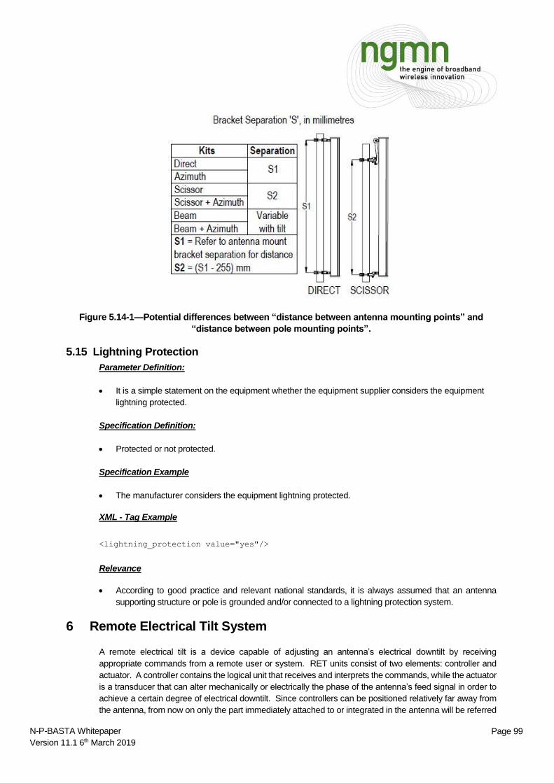
t
Page 99 N-P-BASTA Whitepaper
Version 11.1 6th March 2019
Figure 5.14-1—Potential differences between “distance between antenna mounting points” and
“distance between pole mounting points”.
5.15 Lightning Protection
Parameter Definition:
It is a simple statement on the equipment whether the equipment supplier considers the equipment
lightning protected.
Specification Definition:
Protected or not protected.
Specification Example
The manufacturer considers the equipment lightning protected.
XML - Tag Example
<lightning_protection value="yes"/>
Relevance
According to good practice and relevant national standards, it is always assumed that an antenna
supporting structure or pole is grounded and/or connected to a lightning protection system.
6 Remote Electrical Tilt System
A remote electrical tilt is a device capable of adjusting an antenna’s electrical downtilt by receiving
appropriate commands from a remote user or system. RET units consist of two elements: controller and
actuator. A controller contains the logical unit that receives and interprets the commands, while the actuator
is a transducer that can alter mechanically or electrically the phase of the antenna’s feed signal in order to
achieve a certain degree of electrical downtilt. Since controllers can be positioned relatively far away from
the antenna, from now on only the part immediately attached to or integrated in the antenna will be referred

t
Page 100 N-P-BASTA Whitepaper
Version 11.1 6th March 2019
to as RET. RETs are categorized in fact in three branches: internal, external and partially external. The first
ones are embedded into antennas, while the second ones are typically but not exclusively attached to the
bottom of antennas. The third ones are a particular subset of the external RETs, and are characterized by
being partially inserted into the antenna, and partially protruding outside it.
General RET requirements are specified in the framework of the Antenna Interface Standards Group (AISG)
where specifications for the control interface of antenna devices are defined. RET systems have to operate
in accordance with the AISG standards and with all the relevant part of the 3GPP (Third Generation
Partnership Project) specifications.
In this paper the RET parameters will always be, when not specifically otherwise written, intended as
required.
The format used for the RET parameters will be the same used for electrical specifications and mechanical
specifications.
6.1 Actuator Size
Parameter Definition
The RET stand-alone dimensions.
The RET installed dimensions.
The stand-alone dimensions are defined along the three axis of a Cartesian coordinate system defining
the height (H), the width (W) and the depth (D) of the product (see figure 6.1-1 below).
The installed dimensions are defined along the three axis of a Cartesian coordinate system defining the
height (H), the width (W) and the depth (D) of the product. Installed dimensions are the part of the RET
protruding outside from the RET installation reference plane defined in the antenna datasheet in the
antenna dimensions chapter. (see figure 6.2-1 below).
Figure 6.1-1—Example of an external RET.
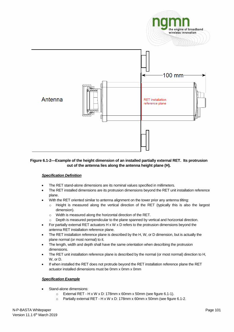
t
Page 101 N-P-BASTA Whitepaper
Version 11.1 6th March 2019
Figure 6.1-2—Example of the height dimension of an installed partially external RET. Its protrusion
out of the antenna lies along the antenna height plane (H).
Specification Definition
The RET stand-alone dimensions are its nominal values specified in millimeters.
The RET installed dimensions are its protrusion dimensions beyond the RET unit installation reference
plane.
With the RET oriented similar to antenna alignment on the tower prior any antenna tilting:
o Height is measured along the vertical direction of the RET (typically this is also the largest
dimension).
o Width is measured along the horizontal direction of the RET.
o Depth is measured perpendicular to the plane spanned by vertical and horizontal direction.
For partially external RET actuators H x W x D refers to the protrusion dimensions beyond the
antenna RET installation reference plane.
The RET installation reference plane is described by the H, W, or D dimension, but is actually the
plane normal (or most normal) to it.
The length, width and depth shall have the same orientation when describing the protrusion
dimensions.
The RET unit installation reference plane is described by the normal (or most normal) direction to H,
W, or D.
If when installed the RET does not protrude beyond the RET installation reference plane the RET
actuator installed dimensions must be 0mm x 0mm x 0mm
Specification Example
Stand-alone dimensions:
o External RET - H x W x D: 178mm x 60mm x 50mm (see figure 6.1-1).
o Partially external RET - H x W x D: 178mm x 60mm x 50mm (see figure 6.1-2.

t
Page 102 N-P-BASTA Whitepaper
Version 11.1 6th March 2019
Installed dimensions:
o External RET - H x W x D: 178mm x 60mm x 50mm (see figure 6.1-1).
o Partially external RET - H x W x D: 100mm x 60mm x 50mm (see figure 6.1-2).
o Integrated RET - H x W x D: 0mm x 0mm x 0mm.
XML - Tag Example
<dimensions height="178" width="60" depth="50"/>
<protrusion height="100" width="60" depth="50"/>
<RET unit installation reference plane= “H”/>
Relevance
The RET actuator dimensions are relevant to plan detailed antenna installations regarding required
space, required fixation points and visual impact.
The RET dimensions may also impact the wind load at a rated wind speed.
t
Page 103 N-P-BASTA Whitepaper
Version 11.1 6th March 2019
6.2 Working Temperature Range
Parameter Definition
The temperature range in which the RET can operate properly, without suffering permanent damage.
It shall also survive without being mechanically or electrically affected due to temperature in any way
that would require service maintenance at the site.
Specification Definition
Nominal values in Celsius degrees.
Minimum and Maximum operating temperatures.
Specification Example
Minimum temperature = -20°C; Maximum temperature = +60°C.
XML - Tag Example
<working_temperature_range max="60" min="-20"/>
Relevance
The RET working temperature range is relevant to evaluate the overall operational working
temperature of the RET system and ensure its correct operation.
6.3 Power Consumption
Parameter Definition
The RET’s consumption of energy.
Specification Definition
Nominal values in Watts.
Values specified for low- and high-power modes.
Definitions of low- and high-power modes according to the relevant 3GPP specification.
Specification Example
Low power consumption = 0.5W; High power consumption = 5W.
XML - Tag Example
<power_consumption high_power="5.0" low_power="0.5"/>
Relevance
The RET power consumption is relevant to estimate a correct overall energy economy.

t
Page 104 N-P-BASTA Whitepaper
Version 11.1 6th March 2019
6.4 Loss of Position on Power Failure
Parameter Definition
This parameter defines, in accordance to the relevant part of AISG standard, whether the RET loses
its position in the event of a power failure during the movement of its motor.
Specification Definition
True / False.
Specification Example
True
XML - Tag Example
<lose_position_on_power_failure value="true"/>
Relevance
In case the position is lost, it is necessary to set the electrical tilt of the RET again whenever the
power is re-established.
6.5 Compatible Standards
Parameter Definition
List of standards which the RET is fully compliant to.
Specification Definition
Standards names can be written in multiple fashions (e.g.: upper or lower case letters, version
specification beginning with “v” or nothing at all). It is the task of the datasheet’s provider to write the
name and version of the standards understandably, while it is the end-user’s task to correctly interpret
them.
The character sequence of: space, semicolon and space shall only be used to separate the string of a
standard from the following one.
Specification Example
RET is compliant with AISG v1.1 and v2.0.
XML - Tag Example
<compatible_standards value="aisg v1.1 ; AISG2"/>
Relevance
Compliance to standards is relevant for RET installation and controlling.
t
Page 105 N-P-BASTA Whitepaper
Version 11.1 6th March 2019
6.6 Compatible Proprietary Protocols
Parameter Definition
List of proprietary protocols which the RET is fully compliant to.
Specification Definition
Protocols names can be written in multiple fashions (e.g.: upper or lower case letters, version
specification beginning with “v” or nothing at all). It is the task of the datasheet’s provider to write the
name and version of the protocols understandably, while it is the end-user’s task to correctly interpret
them.
The character sequence of: space, semicolon and space shall only be used to separate the string of a
protocol from the following one.
Specification Example
RET is compliant with the proprietary protocols of the companies A and B.
XML - Tag Example
<compatible_protocols value="a proprietary ; B_company"/>
Relevance
Important to handle the refarming of the sites where the old RET systems are maintained with
proprietary protocols.
6.7 Configuration Management
Parameter Definition
This parameter defines how the RET configuration is managed. It is applicable to all RETs, internal
and external.
The applicable values are specific to internal or external RETs.
It is possible that some internal RETs might require field configuration, while some internal RETs
might be fixed (not field replaceable).
RETs may be delivered with configuration already loaded (pre-configured). If “not pre-configured” is
noted, then configuration is required (loading the configuration file) before the RET can be operational.
Pre-configured means the RET comes from factory equipped with the appropriate configuration file,
no configuration process is required.
Automatically configuring means the RET will detect the antenna to which it will be connected and
automatically configure itself to work with that antenna, no configuration process is required.
Specification Definition
Only the following values are accepted:
o ”External RET, not pre-configured”
o “External RET, pre-configured”
o “External RET, automatically configured”
o “Integrated RET, not pre-configured”
o “Integrated RET, pre-configured”
t
Page 106 N-P-BASTA Whitepaper
Version 11.1 6th March 2019
o “Integrated RET, automatically configured”
Specification Example
RET is external and not pre-configured.
XML - Tag Example
<configuration_management value="external ret, not pre-configured"/>
Relevance
This parameter is relevant to the operators involved in setting and configuring the RET to a specific
antenna mode for RET position movement.
6.8 Antenna Configuration File Availability
Parameter Definition
This parameter defines whether the configuration file for a specific antenna is available or not. For
specific antennas the manufacturer provides (when available) the antenna configuration file. This
typically happens during the delivery process or during operation.
Specification Definition
True / False.
Specification Example
False.
XML - Tag Example
<antenna_configuration_file_available value="false"/>
Relevance
This parameter is only relevant for a specific antenna model. As an example, in case of need to
substitute the antenna, the manufacturer should be able to provide the relevant configuration file.
6.9 Antenna Configuration File Upgradability
Parameter Definition
This parameter defines whether the configuration file for a specific antenna is upgradable and in that
case specifies how.
This parameter typically applies to external RETs, and RETs that require configuration in the field.
Specification Definition
Only the following values are accepted:

t
Page 107 N-P-BASTA Whitepaper
Version 11.1 6th March 2019
o “Yes, by base station only”
o “Yes, by proprietary portable controller only”
o “Yes, by base station and proprietary portable controller”
o “No”
Specification Example
RET configuration file can be updated both from the base station and from the proprietary portable
controller.
XML - Tag Example
<antenna_configuration_file_upgradable value="yes, by base station and
proprietary portable controller"/>
Relevance
RETs that can be installed and/or configured for an antenna in the field might require configuration per
one of these methods.
6.10 Software Upgradability
Parameter Definition
This parameter defines whether the RET operative system software is upgradable and in that case
specifies how.
Specification Definition
Only the following values are accepted:
o “Yes, by base station only”
o “Yes, by proprietary portable controller only”
o “Yes, by base station and proprietary portable controller”
o “No”
Specification Example
RET software cannot be upgraded.
XML - Tag Example
<software_upgradable value="no"/>
Relevance
For a RET that allows the software to be upgraded in the field, this defines the available methods for
upgrading the software.
6.11 Replaceability in Field
Parameter Definition
t
Page 108 N-P-BASTA Whitepaper
Version 11.1 6th March 2019
This parameter defines whether the RET is replaceable (can be mounted/dismounted) in the same
environment where the antenna is operating. In that case specifies if it is possible only by removing
the antenna from its support, or if this activity may take place without this operation.
Specification Definition
Only the following values are accepted:
o “Yes, without removing antenna”
o “Yes, only removing antenna”
o “No”
Specification Example
RET can be replaced in the field, but in order to be able to do it, the antenna to be removed from its
support.
XML - Tag Example
<field_replacement_allowed value="yes, only removing antenna"/>
Relevance
This parameter is relevant to the operators involved in maintenance and installation of RETs.
6.12 Visual Indicator Available on Tilt Change
Parameter Definition
This parameter defines whether operators within a reasonable distance to the RET are able to be
visually notified when a change of downtilt takes place.
The beginning and the end of the procedure shall be recognizable.
If the RET is not integrated, the visual indicator shall be visible by looking at its external surface.
If the RET is integrated, the visual indicator shall be visible by looking at the external surface of the
RET or of the antenna.
For some antenna models, the visual indicator may be part of the antenna, and thus associated with
the antenna.
Specification Definition
True / False.
Specification Example
False.
XML - Tag Example
<visual_indicator_available_on_tilt_change value="false"/>

t
Page 109 N-P-BASTA Whitepaper
Version 11.1 6th March 2019
Relevance
This parameter is relevant to the operators involved in maintenance and testing of RETs.
6.13 Daisy Chain Available
Parameter Definition
This parameter defines whether it is possible to connect the RET to another one via daisy chain. Specification Definition
True / False.
Specification Example
False.
XML - Tag Example
<daisy_chain_available value="false"/>
Relevance
This parameter is relevant to the operators involved in the installation of RETs and to those
responsible for the correct functioning of a whole cell.
6.14 Smart Bias-T Available
Parameter Definition
This parameter defines whether the antenna is configured with a Smart Bias-T Specification Definition
SBT available True / False.
SBT assigned RF port
Specification Example
False.
XML - Tag Example
<smart_bias_t_available value="false"/>
<smart_bias_t_assigned_port value="3"/>
Relevance
This parameter is relevant to the operators involved in the installation of RETs and to those
responsible for the correct functioning of a whole cell.

t
Page 110 N-P-BASTA Whitepaper
Version 11.1 6th March 2019
7 Environmental Standards
7.1 Base Station Antenna Environmental Criteria
The operating environment of base station antennas is classified as remote, stationary, outdoor,
uncontrolled and not weather-protected. The electromagnetic environment includes close proximity to
intentionally radiating devices and installation on structures prone to lightning strikes. The systems are
expected to operate in this environment for an extended period of time. This, together with storage, transport
and installation conditions, defines the “mission profile” for antennas and other tower top systems – a key
factor needed to their determine reliability.
ETSI defined climatic classifications to describe the operating environment for tower top systems.
Considering that installation environments vary, an antenna cannot fit in only one group, because those
depend highly on the installation area. A summary of these classifications is given in the following table:
Class 4.1 represents a nominal uncontrolled outdoor environment.
Class 4.1E extends temperature and humidity ranges to the average minimum and maximum
temperatures in the 5 European climatic zones.
Classes 4.2L and 4.2H represent more extreme climates addressed by ETSI, but these are also further
extended in regions outside of Europe.
For example, high temperature operation at +70ºC is a common requirement for base station antennas.
Environmental Parameter Classes
Unit 4.1 4.1E 4.2L 4.3H
Minimum air temperature -33 -45 -65 -20 ºC
Maximum air temperature 40 45 35 55 ºC
Minimum relative humidity 15 8 20 4 %RH
Maximum relative humidity 100 100 100 100 %RH
Minimum absolute humidity 0.26 0.03 0.003 0.09 g/m3
Maximum absolute humidity 25 30 22 36 g/m3
Rain intensity 6 15 15 15 mm/min
Maximum temperature change rate 0.5 0.5 0.5 0.5 ºC/min
Minimum air pressure 70 70 70 70 kPa
Maximum air pressure 106 106 106 106 kPa
Solar radiation 1120 1120 1120 1120 W/m2
Maximum wind speed 50 50 50 50 m/s
Table 7.1-1—ETSI 300 019-1-4 stationary, non-weather protected environmental classes.
The standard BSA product complies to the ETSI EN 300019-1-4 standard for environmental conditions:
Class 4.1 E but, as already mentioned, customer requirements and application scenarios might call for more
rigid environmental class compliance such as 4.2L or 4.2H. The specific design changes and material
selections required for that compliance is out of the scope of this whitepaper.
Standard BSAs comply also with:
ETSI EN 300019-1-1 for storage: Class 1.2 (see Section 6.3.1).
ETSI EN 300019-1-2 for transportation: Class 2.3.

t
Page 111 N-P-BASTA Whitepaper
Version 11.1 6th March 2019
Should the standards be updated, or should better standards be available, the
recommendation is to use those instead.
7.2 Environmental Test Approach
The generic test approach for qualifying BSA products is similar to other technical qualification best practice
rules. Overall target is to demonstrate compliance to the applicable standard and one of its environmental
classes.
This qualification requires for each of the environmental parameters (see table above):
A defined test setup: this serves as instruction to set the test up in a defined reproducible way using
certified test equipment. It consists typically of a plan or block diagram identifying the components and
devices of the whole setup, their serial numbers and a wiring diagram. The start settings and/or
calibration procedure of the above mentioned equipment shall also be included.
The definition of standard atmospheric conditions (see IEC 60068) in which the tests take place (even
if during test the specimen might be subject to strongly deviating conditions). These are defined as
ranges to enable testing in environments not completely climatic controlled.
A uniform and reproducible method of environmental test: the procedures of IEC 60068 cover the
different environmental parameters applicable to BSA.
Trained test operator(s) proficient in the usage of test equipment and measurement devices.
A defined number of test specimens. This is rarely prescribed by IEC 60068, but the testing team
should consider this in relation to the test reproducibility: the test might fail or pass by cause of different
devices production techniques, materials, number of suppliers, etc. In case the test effects have some
statistic behavior, the number of test specimen should be selected accordingly (under consideration of
test efforts in time and budget).
A defined set of acceptance criteria. The test specimen shall comply to the defined acceptance criteria
prior and after the test. These criteria are also to be observed and rated during the test itself. Available
test equipment might limit the “during the test” assessment, so a practical but also documented
approach on what is required and what can be done is necessary. The list of acceptance criteria differs
by parameter: for environmental performance ones it typically includes functional tests, electrical
measurements and visual inspection.
A test documentation. This consists of the raw test data and protocols rating the actual measured
values against the test criteria, the identification of the tested specimen (e.g.: by model number and
serial number) and finally the test report. It documents the compliance of the tested devices prior the
tests, specific test events, observations, consolidated data of the test itself and the device compliance
to the acceptance criteria after the test was performed. The report is then concluded by an assessment
of the test results, a compliance statement and a conclusion.
7.3 Environmental Test Methods
The following criteria are used to demonstrate that base station antennas can operate as needed (hence all
the parameters given in the datasheet are valid) in the environments in which they will be typically set in
operation. These tests alone cannot, though, determine an antenna‘s reliability, which is the probability over
time that it will continue to operate as needed in these environments. However, they can establish the initial
reliability and indicate a measure of an antenna’s service life. The aforementioned criteria are based on
publicly available and widely accepted test methods (generally on ETSI Class 4.1 for common performance
needs under nominal conditions or Class 4.1E for extended use – 10 or more years – in harsher
environments).
Comparing the standard ETS300019-2-4 with the IEC60068 it is clear that the characteristic severities of
the ETS might deviate from the corresponding ones of the IEC. Due to this fact and because in general the
definitions of the standards should be sanity-checked considering the BSA application, this whitepaper
recommends test limits that may deviate from corresponding ETS and IEC recommendations.

t
Page 112 N-P-BASTA Whitepaper
Version 11.1 6th March 2019
7.3.1 Packaged Storage
While packaged, transported and stored, antennas shall tolerate non-temperature-controlled-weather-
protected-environments without degradation (Baseline: ETS 300 019-1-1 Class 1.2; -25 to +55°C; 10% to
100% Relative Air Humidity). The conditions for water from sources other than rain are the limiting factor
for the environmental class of packaged storage. The higher ETS 300 019-1-1 classes 1.3 and 1.3E include
splashing water also from side or bottom directions, but since the antennas are packed in cardboard boxes
that normally draw water, get wet and soften up until they rip apart, the packaged storage class shall be
limited to the class 1.2.
7.3.2 Cold Temperature Survival
Antennas shall operate within their specifications after exposure to cold air temperature following IEC 60068-
2-1 test methods (Baseline: ETS 300 019-1-4 Class 4.1; 16 hours at -33°C / Extended: ETS 300 019-1-4
Class 4.1E – further extended to 16 hours at -40°C). Due to test equipment limitations it is not possible to
demonstrate the proper antenna operation and/or the behavior of all antenna parameters during the cold
temperature survival test. The operation of the device is verified prior and following to the test.
7.3.3 Hot Temperature Survival
Antennas shall operate within their specifications after exposure to hot air temperature following IEC
60068-2-2 test methods (Baseline: ETS 300 019-1-4 Class 4.1; 16 hours at +40/55°C / Extended: ETS
300 019-1-4 Class 4.1E – further extended to 16 hours at +60°C). Due to test equipment limitations it is
not possible to demonstrate the proper antenna operation and/or the behavior of all antenna parameters
during the cold temperature survival test. The operation of the device is verified prior and following to the
test.
7.3.4 Temperature Cycling
Antennas shall operate within their specifications after exposure to temperature cycling following IEC 60068-
2-14 test methods (Baseline: ETS 300 019-2-4 Class T4.1; 2 cycles with T1 = 3h and 0.5 °C/min from -10°C
to +40°C / Extended: ETS 300 019-2-4 Class T4.1E; 2 cycles with T1 = 3h and 0.5 °C/min from -10°C to
+45°C).
The characteristic severity of the lower temperature of ETS300019-2-4 strongly differs from the one defined
in the cycle testing of IEC 60068-2-14, but considered that technically the risk for failures increases in the
lower end of the temperature range, and having acknowledged the testing capabilities, this whitepaper
recommends, as a proper compromise between the ETSI and the IEC requirements, applying 5 cycles from
-25 to +45 °C allowing temperature change rates of 1 °C/min.
7.3.5 Vibration – Sinusoidal
Antennas shall operate within their specifications after (non-operating) exposure to sinusoidal vibration
following IEC 60068-2-6 test methods (Baseline: Five 2-200 Hz sweeps in each X, Y and Z axis, limited to
0.5g / Extended: Five 2-200 Hz sweeps in each X, Y and Z axis, limited to 1.0g). This whitepaper
recommends 5 Hz as minimum frequency due to test equipment limitations.
t
Page 113 N-P-BASTA Whitepaper
Version 11.1 6th March 2019
7.3.6 Humidity Exposure
Antennas shall operate within their specifications after (non-operating) exposure to humidity exposure
following the IEC 60068-2-30 test methods (Baseline: 2 cycles between 25 and 40C in 24 hours at 90-98%
relative humidity / Extended: 2 cycles at 30C in 24 hours at 90-98% relative humidity) or their equivalent.
The joint experience is that no failures have been ever observed for these tests. Thus, it is considered to
be a low risk parameter that could be verified with a shorter standard test of 2 cycles/8 hours. In the case
where a new design with major design changes and/or different materials is tested, the experts teams shall
instead apply the more rigid 6 cycles/24 hours testing.
7.3.7 Rain
Antennas shall operate within their specifications after (non-operating) exposure to simulated rain following
the IEC 60068-2-18 test methods (Baseline: ETS 300 019-1-4 Class 4.1: 6 mm/minute for 30 min /
Extended: ETS 300 019-1-4 Class 4.1E: 15 mm/minute for 30 min).
Requirements of 10 mm/min for 30 minutes are in this whitepaper considered an acceptable compromise
between the ETS and IEC characteristic severities.
7.3.8 Water Ingress
Antennas electronics and RF path interconnections potentially exposed to water shall be protected against
splashed, sprayed or windblown ingress to a rating of IPX6 as defined by IEC 60529 “degrees of protection
provided by enclosures (IP Code)”.
This whitepaper recommends the value not to be stated in the technical customer documentation and
datasheets, because only very rarely a customer inquires on this. It is seldom tested and the applicable
class might be directly limited by design features (e.g.: rain drop holes).
7.3.9 Dust and Sand Ingress
Antenna components potentially harmed from dust or sand exposure shall be protected from their ingress
to a rating of IP5X as defined by IEC 60529 “degrees of protection provided by enclosures (IP Code)”
(Baseline: an IP5X dust ingress rating may be assumed without testing based on demonstration of an IPX6
water ingress rating / Extended: IEC 60068-2-68 Test Lc1 or the equivalent).
Overall, this is not considered to be a problem. It is extremely rarely tested, and if inquired, the figure might
be deducted from the water Ingress test figure. This whitepaper recommends the value not to be stated in
the technical customer documentation and datasheets.
7.3.10 Survival Wind Speed
Antennas shall survive exposure to forces simulating the effects of strong winds according to the definition
in Section 5.8. It is calculated using methods consistent with Eurocode 1 “Actions on structures” – Part 1-4
“General actions” – “Wind actions” (EN 1991-1-4) and/or EIA/TIA 222-G (Baseline: 50 meters/sec 180 km/h
or 112 mph / Extended: 50 meters/sec 180 km/h or 112 mph). The detailed reference to be used might vary
by country and has to be checked accordingly.
The maximum wind velocities cited in ETS 3000019 are not considered to be sufficient for BSA applications.
Consequently and in line with the customer requirements a standard survival wind speed of 200 km/h is

t
Page 114 N-P-BASTA Whitepaper
Version 11.1 6th March 2019
defined. For higher windload designs typically 240 km/h is realized although individual customer tailored
design solutions might be required. It is acceptable to demonstrate compliance to this survival wind speed
by:
Dynamic testing.
Static testing.
FEM modeling & simulation.
Similarity to existing verified products.
Analytics applying best structural engineering practices.
This whitepaper recommends: 55.6 meter/sec; 200 km/h (124 mph) for standard duty antennas, 66.6
meters/sec 240 km/h (150 mph) for heavy duty antennas.
7.3.11 Solar/Weather Exposure
Antenna materials shall not degrade significantly after simulated solar exposure following the IEC 60068-2-
5 test methods or their equivalent. The IEC defines three different methods with two cyclic (cycle of light
and dark) and one continuous radiation exposure. The cyclic tests are considered to be more aggressive,
especially the procedure B that has 20 hours light and only 4 hours dark time (Baseline: 20 hours on / 4
hours off at 55°C for 56 cycles/56 days = 1344 hours).
In order to save time, shortening the test duration was discussed. Experience is that test duration of at least
1000 hours shows the material failures and that the test samples have to be visually inspected. Moreover,
some mechanical tests (tensile and/or bending) have to be performed to ensure the materials keep at least
60% their initial properties and do not get brittle. The standards define detailed lists of light sources qualified
for the test with resulting impact on test conditions (typically the wavelength of the UV is applied). Any light
source compatible with the above mentioned cycling procedure B is acceptable.
Crack, chalking or permanent dimensional change might appear in any intermediate test or final inspection.
The individual material changes that might be tolerated depend on the material and where it is used: this is
to be risk assessed by the mechanical designer on a case by case basis; therefore no generic applicable
guidance can be provided in this whitepaper. As an example, these material specific limits could be defined
considering following behavior as a failure of the material:
Mean tensile strength change > 10%
Mean elastic modulus change > 30%
Mean elongation change > 30%
Mean impact strength change > 30%
Remark: Significant color changes completely changing the visual aspect of the antenna could become an
issue for customer acceptance even if they would not negatively impact the environmental reliability of the
antenna.
7.3.12 Corrosion Resistance
Antenna materials and surface finishes shall be corrosion resistant for the intended service lifetime. The
system, or its components and materials, shall be tested for corrosion resistance following the IEC 60068-
2-11, test Ka method (a.k.a. B117) using a salt fog (mist) from a neutral, 5% weight sodium chloride solution
for 28 days = 720 hours (Standard Baseline: 10 days = 240 hours / Extended: “Procedure B” with 20 hours
on / 4 hours off at 40°C for 28 days = 672 hours).

t
Page 115 N-P-BASTA Whitepaper
Version 11.1 6th March 2019
Functional tests shall be done prior to and after the corrosion exposure. The visual acceptance criteria are
many and require some definition. While it is jointly agreed that after 28 days of salt spray testing there are
always some ‘salt’ remains on the device (which is acceptable), corrosion starting at metal parts is not
acceptable.
Due to limitations of test equipment it is not feasible to test complete antenna products in all cases. Suitable
test samples are typically selected to demonstrate the viability versus salt corrosion of the antenna including
all connectors, sealings, materials, joints and moving parts. This whitepaper recommends the test duration
defined in IEC 60068-2-11 ranges from 16 hours to 672 hours = 28 days, but individual customer inquiries
asking for even longer test durations might occur.
Acceptance criteria (visual inspection shall be done before and after test):
Excessive corrosion in critical areas.
Salt deposits in electrical critical areas.
Corrosion of insulating materials and metals.
Clogging or binding of movable parts.
After completing the test, the exposed materials may be washed with warm water and lightly brushed to
remove the salt deposits and expose the base material under the salt.
The following are indications of material failure:
The base material has been attacked by the salt deposits.
In the case of plating, bubbling, lifting or the plating has been eaten through.
For assemblies with working mechanical pieces, failures of thread, seals, etc.
Leakages.
Illegibility of marking and nameplate.
Moreover, electrical measurements have to be done before and after test (if applicable) to assess:
VSWR.
Isolation.
Intermodulation.
7.3.13 Shock & Bump
An antenna shall survive shocks and/or bumps without suffering any permanent damage that can alter its
electrical and/or mechanical features, compromising its service efficiency. Visual and operational checks
are to be done prior to and after the shock & bump trial in order to verify whether the antenna has maintained
its charateristics. The test method is indicated by IEC 60068-2-27 “Test Eb: Bump” (Baseline: antenna
without packaging, half-sine bumps from 6 directions, 100 bumps in each direction).
This whitepaper recommends applying, irrespective of the product weight, the test specifications below:
Antenna Weight Input Acceleration Duration
<50kg 100 m/s² 6 ms
>50kg 50 m/s² 11 ms
7.3.14 Free Fall (Packaged Product)
An antenna shall survive free falls without suffering any permanent damage that can alter its electrical and/or
mechanical features, compromising its service efficiency. Visual and operational checks are to be done

t
Page 116 N-P-BASTA Whitepaper
Version 11.1 6th March 2019
prior to and after the free fall trial in order to verify whether the antenna has maintained its charateristics.
The test method is indicated by IEC 60068-2-31 (Baseline: packaged antenna, 1 fall per face or 2 falls,
altitude specified in the table below).
Mass [kg] Free fall test height [m]
Class T 2.2
Free fall test height [m]
Class T 2.3
< 10 0.8 1.0
< 20 0.6 0.8
< 30 0.5 0.6
< 40 0.4 0.5
< 50 0.3 0.4
< 100 0.2 0.3
> 100 0.1 0.1
Table 7.3-1—Free fall test heights.
This whitepaper recommends this either to be tested, or to declare the compliance referring to existing test
results of products with similar packaging design. The test shall also be only applied for the 6 flat sides of
the package (no corner drop test is applied).
7.3.15 Broadband Random Vibration
An antenna shall survive random vibration within a broad spectrum without suffering any permanent damage
that can alter its electrical and/or mechanical features, compromising its service efficiency. Visual and
operational checks are to be done prior to and after the vibration trial in order to verify whether the antenna
has maintained its charateristics. The test method is indicated by IEC 60068-2-64 “Test Fh: Vibration
broadband”.
This whitepaper recommends the tested frequency spectrum for broadband random vibration to be aligned
with the one applied for the sinusoidal testing (see Section 7.3.5).
7.3.16 Steady State Humidity
Antenna materials and surface finishes shall be humidity resistant for the intended service lifetime. The
system, or its components and materials, shall be tested for steady state humidity following the test method
designated by IEC 60068-2-56 “Test Cab : Damp Heat, Steady state” (Baseline: 93% relative humidity, with
a temperature of +40°C ± 2°C and a duration of 21 days = 504 hours).
The steady state humidity test according IEC 60068-56 allows different combinations of temperature and
relative humidity and test durations in a range from 12 hours to 1344 hours = 56 days. The selected
parameters above define a very stringent (highest temperature combined with highest relative humidity,
second longest test duration) test condition, which is recommended by this whitepaper too.
8 Reliability Standards
Reliability is the probability that a product or service will perform as needed for a specified time and under
specified operating conditions. It deals with the knowledge of the physics of failure and with the design to
reduce it throughout the product’s service life or, for complex systems such as antennas, to make them
tolerant to failures when they do happen. Acceptance and qualification tests address initial quality by
showing that no failures occur under certain operating and environmental conditions. While these conditions

t
Page 117 N-P-BASTA Whitepaper
Version 11.1 6th March 2019
may include “reliability demonstrations” (such as corrosion tests run for a fixed time), these tests cannot
determine a product’s reliability.
By contrast, reliability tests are meant to actually cause failures, usually by “accelerating product aging”, so
that realistic failures happen quickly. These tests are designed to measure failure rates (or MTBF values)
and operating lifetimes. While there are many references for general reliability test methods (the IEC 60605
family of standards is one example), in practice most reliability tests and predictions are customized around
product features and dominant failure mechanisms. As a result failure rates, MTBF values and lifetimes are
always approximations under several assumptions, which shall be known and understood to properly
compare predictions from different sources.
9 Additional Topics
9.1 Recommended Sub-bands and Associated Frequency List
From the operators point of view it is an ordinary procedure to require that antennas produced by vendors
are measured by very specific frequencies of interest. This routine represents a huge problem in the
economy of the vendors, which ultimately results in longer wait times and higher costs for everyone. It also
denies an accurate comparison between antennas, since there is no assurance that similar antennas from
different vendors are measured by the same frequency points. Thus it is critical that all the parties involved
in the evaluation of antennas use an agreed upon set of frequencies for the calculation of antennas’
parameters.
Frequency bands for mobile telecommunications are highly standardized by organizations such as ETSI
and 3GPP, hence here it will not be necessary to define them anew. This whitepaper will in fact refer to the
latest operating bands table (at the time of this document’s writing it was contained in section 4.5.1 of the
3GPP TS 37.104, v14.1.0, 2016-09), an adaptation of which will also be used in the following sections as
an example, or an equivalent one (should the original table not be available or applicable anymore).
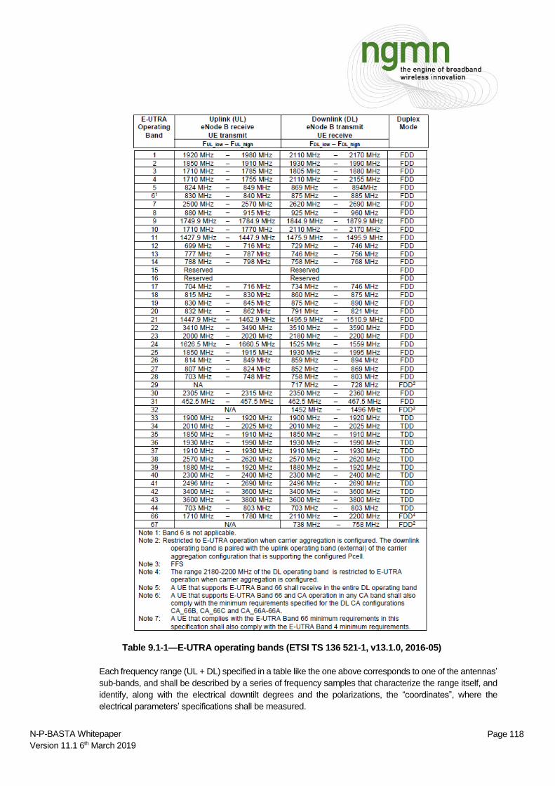
t
Page 118 N-P-BASTA Whitepaper
Version 11.1 6th March 2019
Table 9.1-1—E-UTRA operating bands (ETSI TS 136 521-1, v13.1.0, 2016-05)
Each frequency range (UL + DL) specified in a table like the one above corresponds to one of the antennas’
sub-bands, and shall be described by a series of frequency samples that characterize the range itself, and
identify, along with the electrical downtilt degrees and the polarizations, the “coordinates”, where the
electrical parameters’ specifications shall be measured.
t
Page 119 N-P-BASTA Whitepaper
Version 11.1 6th March 2019
As an example, let an antenna’s electrical downtilt range from zero to two degrees, two polarizations (+45°
and -45°), and let the E-UTRA operating band 31 of previous table be the sub-band to be analyzed. The
values constituting the dataset of the particular 452.5-467.5 MHz sub-band shall then be measured by:
455 MHz, 0° tilt, +45° polarization
465 MHz, 0° tilt, -45° polarization
455 MHz, 1° tilt, +45° polarization
465 MHz, 1° tilt, -45° polarization
455 MHz, 2° tilt, +45° polarization
465 MHz, 2° tilt, -45° polarization
Where 455 MHz and 465 MHz were chosen as characteristic frequency samples to describe the E-UTRA
operating band 31 (the choice method will be elaborated in the following sections).
It is critical to acknowledge that the spectrum “evolves” and that a frequency table is very unlikely to remain
unchanged throughout the time. Considering that at the time of this document’s writing there was no
standard or technical guideline defining a method to measure antennas through the use of specific frequency
samples for each sub-band, it is impossible here to refer to another source or recommend a list of fixed
frequencies, without having to update it each time a new table is published. In order to keep this document’s
adaptability to all the frequency tables to come, a “frequency ranges choice algorithm” and a “frequency
samples choice algorithm” have been developed to be here recommended.
The proposed algorithms is a dynamic (innovation-resistant) one, and it was built around constraints defined
by the fact that it is either very expensive, time-consuming and equipment-dependent to measure broadband
antennas with simpler techniques, or very inaccurate to do it. For example, using a fixed “frequency step”
(e.g.: measuring a 1710-2690 MHz band every 10 MHz), could require either too many (98 in this case)
frequency samples – this would mean using expensive equipment and waiting longer for a measurement to
end –, or only a few (e.g.: 25 samples, which is a much more reasonable number, would require a sample
every 39.2 MHz), with the risk of representing antennas with a single “weak” or “strong” pattern for a broad
specific frequency neighborhood (antennas’ patterns change already in 20 MHz, in this case a single
frequency would be used to be representative of almost two times the width).
9.1.1 Frequency Ranges Choice Method
The first steps of this algorithm consist in:
Finding the most recent frequency table (see previous section).
Copying the UL range in the DL column when the DL is marked by “N/A” (see Table 13) and vice versa.
Approximating the frequency ranges to the nearest unit of megahertz.
Sorting the table “horizontally”, by defining “lowest” and “highest” portion of sub-bands, regardless of
UL or DL.
Sorting the table “vertically” in ascending fashion, giving priority to the lower start-frequency and, in the
case of match, to the narrower band (total broadness of lowest + highest portions), and finally to the
order of appearance (band number) in the original frequency table.
With reference to Table 13, the following should be obtained as results here:

t
Page 120 N-P-BASTA Whitepaper
Version 11.1 6th March 2019
Table 9.1-2—Sorted frequency table.
At this point a deeper analysis of the table is necessary. Before selecting each sub-band’s representative
samples, it should be noticed that some of these sub-bands are contained in others and some overlap each
other. In these cases, the method proposed in this whitepaper contemplates a unification of the sub-
bands in accordance to the following set of rules:

t
Page 121 N-P-BASTA Whitepaper
Version 11.1 6th March 2019
Each sub-band in the sorted table shall be compared with the immediately following one.
Should the application of these rules result in a “merged” band, this one shall be immediately considered
for the next comparison.
If a band is completely contained in another one, the broader will represent them both and keep all its
characteristics. Exceptions to this rule are sub-bands, which are only contained in another’s band-gap
(between the lowest and highest portions of the sub-band), and those whose total bandwidth is narrower
than half the other’s width.
Example: sub-band 44 and 17 are compared. The first one has no band gap, while the second one has a
gap between 716 MHz and 734 MHz; the total bandwidth of sub-band 17 is 90 MHz, while band 44 is 100
MHz broad (sub-band 17 is >= 50% of band 44’s width). Sub-band 44 contains sub-band 17 totally and
none of the exceptions are verified. A new sub-band called “17+44” will take place of the two merged ones
and will extend from 703 MHz to 803 MHz. Per the second point, the sub-band 17+44 shall then be
compared to sub-band 29.
If at least the 70% of a sub-band is contained in another, a new one will represent them both. In this
case its start frequency shall be the lowest amongst the two analyzed sub-bands, by analogy the stop
frequency shall be the highest instead. If both the merged sub-bands contain a band-gap, the new sub-
band will too contain a gap, which will split the sub-band in lowest and highest portion. This new gap
shall be the “common gap”, that is the spectrum that does not contain any bit of any portion of any of
the two analyzed sub-bands.
Example: Sub-Band 18 overlaps with sub-band 5. The overlapping ranges are 824-830 MHz in the lower
portion and 869-875 MHz in the higher portion of the sub-bands. The total overlapping spectrum is 12 MHz,
which is the 40% of the sub-band 18 and 13.3% of sub-band 5. In this case the sub-bands are not merged
(none of them reaches 70%), but if they were, the common gap would have been 849-860 MHz and the
new sub-band would have been the “18+5”, whose portions would have been 815-849 MHz and 860-894
MHz.
Finally, if the total width of a sub-band is lower or equal than 30 MHz, and it has a difference from
another sub-band of no more than 10 MHz between start frequencies and/or end frequencies of both
the portions, the narrower sub-band shall be merged with the broader one. In this case, regardless of
the overlapping percent, the procedure to follow is described in the previous point.
These rules shall be applied over again, until no bands can be merged anymore.
After this process, the frequency table should look as follows:
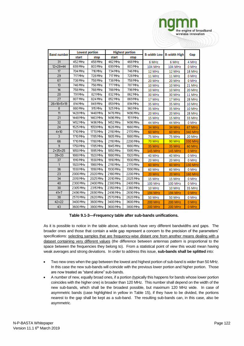
t
Page 122 N-P-BASTA Whitepaper
Version 11.1 6th March 2019
Table 9.1-3—Frequency table after sub-bands unifications.
As it is possible to notice in the table above, sub-bands have very different bandwidths and gaps. The
broader ones and those that contain a wide gap represent a concern to the precision of the parameters’
specifications: selecting samples that are frequency-wise distant one from another means dealing with a
dataset containing very different values (the difference between antennas pattern is proportional to the
space between the frequencies they belong to). From a statistical point of view this would mean having
weak averages and strong deviations. In order to address this issue, sub-bands shall be splitted into:
Two new ones when the gap between the lowest and highest portion of sub-band is wider than 50 MHz.
In this case the new sub-bands will coincide with the previous lower portion and higher portion. Those
are now treated as “stand alone” sub-bands.
A number of new, equally broad ones, if a portion (typically this happens for bands whose lower portion
coincides with the higher one) is broader than 120 MHz. This number shall depend on the width of the
new sub-bands, which shall be the broadest possible, but maximum 120 MHz wide. In case of
asymmetric bands (case highlighted in yellow in Table 15), if they have to be divided, the portions
nearest to the gap shall be kept as a sub-band. The resulting sub-bands can, in this case, also be
asymmetric.

t
Page 123 N-P-BASTA Whitepaper
Version 11.1 6th March 2019
Example: Sub-Band 4+10 contains a gap of 340 MHz between its lower and higher portions. It will then be
divided in sub-band “(4+10)a” and “(4+10)b”, whose frequency ranges are respectively: 1710-1770 MHz
and 2110-2170 MHz.
Example: Assume sub-band 66 to be 1650-1780 MHz / 2110-2200 MHz. Since its lower portion would be
130 MHz wide and its higher portion 90 MHz wide, the lowest one should be split into two sub-bands: 1650-
1715 MHz and 1715-1780 MHz / 2110-2200 MHz. The second sub-band would be, in fact, the combination
of sub-band 66’s portions nearest to its frequency gap.
Cases in which these divisions take place are highlighted in orange in Table 15. After this process, the
frequency table shall be sorted again (see beginning of this section) and should look as in the table below:
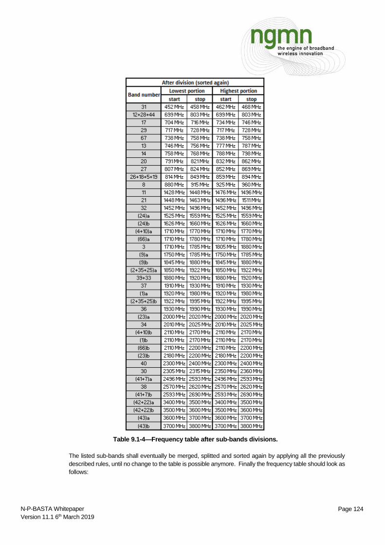
t
Page 124 N-P-BASTA Whitepaper
Version 11.1 6th March 2019
Table 9.1-4—Frequency table after sub-bands divisions.
The listed sub-bands shall eventually be merged, splitted and sorted again by applying all the previously
described rules, until no change to the table is possible anymore. Finally the frequency table should look as
follows:

t
Page 125 N-P-BASTA Whitepaper
Version 11.1 6th March 2019
Table 9.1-5—Frequency table at the end of the merging/splitting/sorting processes.
None of the sub-bands listed above can be merged or splitted. At this time another issue should be
considered: the algorithm described until now works with respect to a frequency table that is already
standardized, but what just stated does not fully comply with the needs of the research & development,
which generally cannot wait the amount of time essential to the processes that result in a standardization of
the frequencies (therefore to a frequency table). Thus, extensions to the sub-bands are here contemplated,
that is an appendix up to 15 MHz wide may be added to a single portion of the sub-bands, whether
before its start frequency or after its stop frequency. Notice that at this point no merging or splitting is
possible anymore, which means that from now on a sub-band may be maximum 135 MHz wide, and/or that
a sub-band may overlap with (hardly contain) another one. For the sake of comprehension, in the table
above the lower portion of the sub-band “(4+10)a+(66)a” will be extended to 1695-1780 MHz:
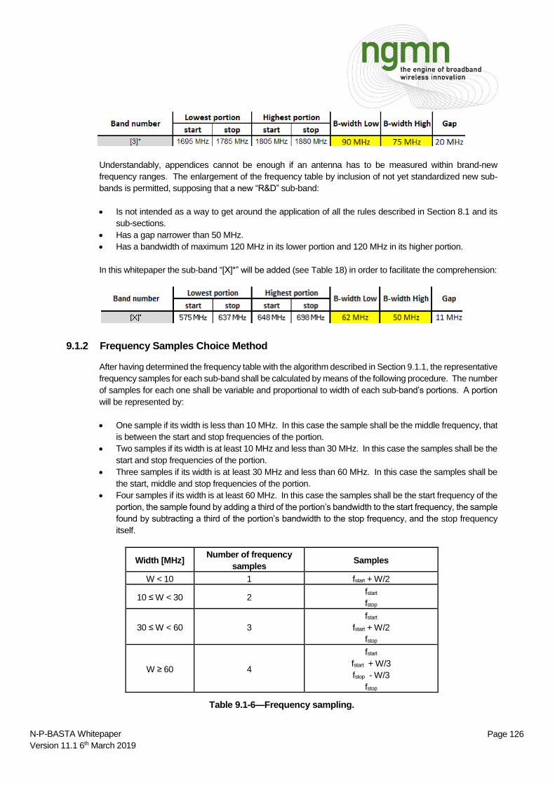
t
Page 126 N-P-BASTA Whitepaper
Version 11.1 6th March 2019
Understandably, appendices cannot be enough if an antenna has to be measured within brand-new
frequency ranges. The enlargement of the frequency table by inclusion of not yet standardized new sub-
bands is permitted, supposing that a new “R&D” sub-band:
Is not intended as a way to get around the application of all the rules described in Section 8.1 and its
sub-sections.
Has a gap narrower than 50 MHz.
Has a bandwidth of maximum 120 MHz in its lower portion and 120 MHz in its higher portion.
In this whitepaper the sub-band “[X]*” will be added (see Table 18) in order to facilitate the comprehension:
9.1.2 Frequency Samples Choice Method
After having determined the frequency table with the algorithm described in Section 9.1.1, the representative
frequency samples for each sub-band shall be calculated by means of the following procedure. The number
of samples for each one shall be variable and proportional to width of each sub-band’s portions. A portion
will be represented by:
One sample if its width is less than 10 MHz. In this case the sample shall be the middle frequency, that
is between the start and stop frequencies of the portion.
Two samples if its width is at least 10 MHz and less than 30 MHz. In this case the samples shall be the
start and stop frequencies of the portion.
Three samples if its width is at least 30 MHz and less than 60 MHz. In this case the samples shall be
the start, middle and stop frequencies of the portion.
Four samples if its width is at least 60 MHz. In this case the samples shall be the start frequency of the
portion, the sample found by adding a third of the portion’s bandwidth to the start frequency, the sample
found by subtracting a third of the portion’s bandwidth to the stop frequency, and the stop frequency
itself.
Width [MHz] Number of frequency
samples Samples
W < 10 1 fstart + W/2
10 ≤ W < 30 2 fstart
fstop
30 ≤ W < 60 3
fstart
fstart + W/2
fstop
W ≥ 60 4
fstart
fstart + W/3
fstop - W/3
fstop
Table 9.1-6—Frequency sampling.

t
Page 127 N-P-BASTA Whitepaper
Version 11.1 6th March 2019
All the samples calculated this way shall be approximated to the nearest unit of megahertz. Below the list
of frequency samples associated to each sub-band:
Table 9.1-7—Samples associated to sub-bands’ portions.
When the lower and higher portions coincide, it means that there is actually only a single “block” of spectrum
occupied by the associated sub-band, hence the samples appearing in both the portions columns are
doubles, and only one occurrence of each one shall be taken into consideration when building the dataset
whose distribution will be analyzed. In this example, the list of frequency samples counts 124 unique
frequencies to measure, in order to be able to evaluate the performances of a hypothetical antenna between
452 MHz and 3800 MHz in 37 different sub-bands.
Though, not every sample is needed. In the table above (and by extension in all the tables built following
the procedures described until now) there are some samples that are very close one another, which means
that there is a certain degree of redundancy that can be reduced through optimization. This shall be
achieved by applying the following rules in their presented order:
Each sample shall be compared to the following ones, after the list of samples is sorted in ascending
fashion.
Frequency samples belonging to “R&D sub-bands” shall always be removed from the list if there is
already a sample 3 MHz or less (see third point) or 10 MHz or less (see fourth point) distant. Those
shall be used instead. This is not applied to “appendices”.
Under 1000 MHz:

t
Page 128 N-P-BASTA Whitepaper
Version 11.1 6th March 2019
o If three or more (the maximum is obviously four) adjacent frequency samples are 3 MHz or less
distant one from each other, and the farthest ones have a difference of exactly 3 MHz, the samples
in the middle shall be removed from the list.
o If, instead, the difference is greater than 3 MHz, the last amongst the adjacent samples shall be
preserved, and another one shall be chosen through a new comparison: if the distance between
the preserved sample and the average between the first two adjacent ones is less than 3 MHz, the
first sample shall be preserved too. Otherwise a new sample shall replace the first two ones, and
its frequency will be equal to their average.
o If two or more (the maximum is obviously three) adjacent frequency samples are less than 3 MHz
distant one from each other, they shall be replaced by a single sample, whose frequency will be
equal to the average of the two farthest replaced ones.
If the cases described in the third point are verified for comparisons between frequency samples under
1000 MHz and above or exactly 1000 MHz, the rules of the third point shall be applied too.
1000 MHz and above:
o If three or more adjacent frequency samples are 10 MHz or less distant one from each other, and
the farthest ones have a difference of exactly 10 MHz, the samples in the middle shall be removed
from the list.
o If, instead, the difference is greater than 10 MHz, the last amongst the adjacent samples shall be
preserved, and another one shall be chosen through a new comparison: if the distance between
the preserved sample and the average between the first two adjacent ones is less than 10 MHz,
the first sample shall be preserved too. Otherwise a new sample shall replace the first two ones,
and its frequency will be equal to their average.
o If two or more adjacent frequency samples are less than 10 MHz distant one from each other, they
shall be replaced by a single sample.
Once samples have been replaced, they shall be rounded to the nearest unit of megahertz. The
replaced ones shall be compared to the next ones in the list.
Below some examples:
Figure 9.1-1—Examples of frequency samples redundancy optimization.
On the left (notice also that 698 MHz is one of the frequencies introduced by the R&D band [X]*) there are
two cases where the highlighted frequency-samples are simply averaged. In the center there are a couple
of “blocks” of samples to optimize one after the other: the first one goes from 1725 MHz to 1750 MHz. Since
1725 MHz and 1733 MHz averaged are more than 10 MHz distant from 1750 MHz, 1729 MHz and 1750

t
Page 129 N-P-BASTA Whitepaper
Version 11.1 6th March 2019
MHz appear in the “final samples” list. The second one goes from 1750 MHz (because it has been
preserved) to 1768 MHz; the rules applied are the same. On the right there are also cases where only the
middle sample is eliminated because the distance between 2 samples is exactly 10 MHz.
At this point, the only thing to do left is to replace the samples listed in Table 18 with the optimized ones. To
do this, each frequency sample nearest to those to be replaced shall take their place. In case two samples
are equally distant from the one to replace, the priority shall be given to the one inside the sub-frequency,
and finally, if both are, to the higher one.

t
Page 130 N-P-BASTA Whitepaper
Version 11.1 6th March 2019
Table 9.1-8—Final frequency table. Samples undergoing optimization are highlighted.

t
Page 131 N-P-BASTA Whitepaper
Version 11.1 6th March 2019
9.1.3 Compatibility with old whitepaper versions and use of non-BASTA frequencies
When a new frequency table is released and the frequency samples accordingly calculated, there can be
two issues yet to deal with:
The calculated frequency samples are not exactly those used by operators all over the world.
Older antennas cannot be exactly compared to newer ones, due to difference in measured frequency
samples.
In case of need, a specific non-BASTA frequency sample and the all the values (parameters, pattern level,
etc.) associated to it can be calculated by linear interpolation between two frequency samples compliant
with the latest version of this whitepaper. The proportion to use are the following:
(Sample A - Sample B) : 100 = (Sample A - Non-BASTA frequency sample) : (100 – x)
(Value by sample A - Value by sample B) : 100 = (Value by sample A - Value by interpolated sample) : x
This option shall be valid only for structures that are non-resonant between the selected frequencies. A
maximum distance of 34 MHz between two frequency samples implicitly defined in this whitepaper
guarantees (antenna’s patterns are different in this neighborhood, but not extremely) a sufficient fidelity of
the values obtained by interpolation to those that would be through a real measurement. Samples obtained
through interpolation shall not be used but for internal purposes, and shall not be included in antennas’
BASTA-compliant datasets.
9.2 Guidance on Pattern and Gain Measurements
A general guideline is that all equipment used for measurements of antennas patterns and gain should be
calibrated with a visible proof of the latest calibration date. The following section give recommendations on
the methodology to observe in order to correctly execute an antenna’s measurement.
9.2.1 Mechanical Alignment of Test System
The mechanical boresight of the antenna and measurement system shall be calibrated by testing the
antenna elevation pattern two times: once with the typical operating setup, while the second time the
antenna mounting shall be rotated by 180 degrees or, if possible, the antenna mounting axis shall be flipped
(recommended). In both cases the value of the measured antenna electrical tilt should be the same;
contrarily, mechanics shall be realigned and tested again.
9.2.2 Phase Center Check
The antenna shall be rotated around its own phase center. To ensure that it happens, a pattern test on the
middle frequency of each cluster shall be run to acknowledge the phase response over the azimuth. The
outcome is a phase curve, which shall be flat in the angular region corresponding to the main beam of the
antenna. If not, the antenna shall be positioned away from or towards the mechanical rotation center of the
system, until it is aligned with the antenna phase center.
9.2.3 Antenna Pattern Testing
The system shall be set up to measure the antenna’s patterns by the frequencies identified through the rules
described in Section 9.1. A unique calibration shall be used for all the antenna’s ports, and the test shall
start from the minimum frequency supported by each cluster of the antenna and shall end with its supported
maximum one. The azimuth and elevation patterns, Co-Pol and Cross-Pol shall be measured for each port

t
Page 132 N-P-BASTA Whitepaper
Version 11.1 6th March 2019
and electrical downtilt of interest (see Section 4.2). These consist in the set of signal levels measured
respectively by every azimuth and elevation degree of interest (see Section 4.2), which appear respectively
in the same elevation and azimuth cuts where the absolute signal maximum lays. Signal levels can be in
this way easily compared and evaluated relatively to each other. The resulting patterns shall have the
antenna’s mechanical boresight as an angular “zero-reference”.
9.2.4 Pattern Accuracy Estimation
The following quick tests shall be performed before any measurement.
When possible, a golden unit antenna with known performance (from another range) shall be tested.
A pattern sweep (360 degrees) shall be run, and the signal level by -180º and +180º shall be checked.
The signal levels should be identical since those point coincide, but they are measured with a time
difference between them. If the signal level is not the same, this shall be taken as an indication of
instability in the measurement setup, or of the surrounding environment. This issue should be further
investigated (loose connections, signal interference, stability in instruments) before starting a
measurement.
A second pattern sweep shall be run with the antenna mounting rotated by 180º. At the end both
patterns shall be checked for symmetry issues (right hand side of pattern in test 1 should look the same
as left hand side of pattern in test 2). This test can give information of asymmetries in the measurement
range (reflections or interfering signals from one direction).
The two steps above are worth to be taken for both azimuth and elevation patterns.
9.3 Gain Measurement
In the following sections two methods to calculate the gain of an antenna will be described.
9.3.1 Gain by Substitution Method
The gain by substitution (also known as gain by comparison) method consists in a procedure that allows to
measure an antenna’s gain by using a reference antenna whose gain is already known, which is then
compared with the AUT. The gain reference antenna is typically a calibrated standard gain horn.
The first step in this procedure consists in calibrating the test range using the gain reference antenna
by positioning it in its phase center and main beam direction, hence giving the system a “zero
reference”. This shall be done for each individual polarization of interest, since the transfer function of
the range can be different for each polarization.
The second step consists in measuring the antenna under test in its phase center and main beam
direction.
The gain of the AUT is finally found by taking the measured values (step two), and adding the known gain
of the reference antenna, which is typically found in a document delivered with it.
9.3.2 Gain by Directivity/Loss Method
An alternative gain measurement procedure is the gain by directivity/loss method. This procedure allows to
measure an antenna’s gain by measuring the directivity of an antenna and then considering its losses. Gain
(G) and directivity (D) are in fact linked by the formula:
DkG

t
Page 133 N-P-BASTA Whitepaper
Version 11.1 6th March 2019
with k representing the antenna efficiency factor (0 k 1), which describes the overall losses of the antenna
(k = 1 means that the antenna is lossless). Therefore the antenna gain can be calculated by:
dBadBDdBG antenna
where a is the sum of all the antenna’s losses.
Measuring the Directivity of an Antenna
To calculate the directivity, the field irradiated from an antenna shall be measured in every direction through
the interaction of the Antenna Under Test (AUT) and a probe. This procedure is better performed with the
entire system placed in an anechoic chamber (typically in near-field conditions) that allows the rotation of
the AUT in both the spherical axis (theta 𝜃 and phi 𝜙).
Figure 9.3-1—Spherical near-field system.
The directivity cannot be measured directly, but shall be computed from the far-field power pattern
normalized to its maximum value:
𝐷 =4𝜋 𝑃𝑛(𝜑𝑚, 𝜃𝑚)
∯ 𝑃𝑛 (𝜑, 𝜃) sin 𝜃 𝑑𝜑𝑑𝜃
where D is once again the directivity and Pn the tridimensional power pattern.
In substance the directivity is calculated from a full tridimensional pattern measurement:
4log10 dBPowersumdBMaxFFdBD
where:
o MaxFF = Overall peak of the measured and computed FF.
o Powersum = Sum of all measured and computed far-field points (3D).
During the calculation of the directivity the following faults can cause problems:
Shadowing effects of the scanner, which unavoidably cause a wrong Powersum to be calculated.
Probe correction error, which causes the software to perform wrong NF to FF transformations.

t
Page 134 N-P-BASTA Whitepaper
Version 11.1 6th March 2019
Insufficient FFT density (sampling criteria should be carefully chosen during scanning and the near-to-
far-field transformation), which causes aliasing.
Wrong FF reference polarization, which causes false patterns to be measured.
High Cr-Pol level in the measurement probe.
Measuring the Internal Losses of an Antenna
The antenna losses are the sum of the ohmic and dielectric losses between the input connector and the
outer surface of the radome plus the loss due to the impedance mismatch:
radomematchantennamisnetworkantenna aaaa
The feeding loss αnetwork can be measured with a network analyzer as shown in the following picture:
Figure 9.3-2—Block diagram of loss measurement.
This measurement shall be executed in four steps:
Radiating elements shall be detached from the network.
The transmission of each input-to-output path shall be measured.
All the transmission losses of each path shall be summed.
αnetwork shall be calculated as the average of the total transmission losses for each path.
The antenna mismatch has to be calculated with the formula:
dBea
RL
mismatch
10
10 1log10
where RL is the return loss.
In the end, the overall network loss is:
mismatchnetworkcomponentscablesnetwork aaaa _
Radiating elements
Electrical components
Network-
analyzer
Connector
Network

t
Page 135 N-P-BASTA Whitepaper
Version 11.1 6th March 2019
The dielectric losses of the radome depend on its loss factor tanδ, which differs for each material. Under
the assumption that the radome is normally thin, the value of tanδ is less than 0.05dB and therefore can be
neglected.
9.4 On the Accuracy of Gain Measurements
The following sections will detail potential sources of errors occurring during an antenna’s gain
measurement, and will give recommendations in order to minimize these errors. This discussion will be
mainly focused on gain measurements done using the method of substitution and by means of far-field
ranges (but its validity is extended to near-field gain measurements).
As a general rule it is strongly advised that all instruments have reached their working temperature before a
calibration or a measurement, and that the measurement equipment is calibrated with the reference antenna
as close in time as possible prior to the gain measurements. After the gain measurements have been
performed, the reference antenna should be mounted and measured again against the previous calibration;
should any deviation from it be observed, this shall be taken as an indication of instability in the measurement
setup, or of the surrounding environment. This issue should be further investigated (loose connections,
signal interference, stability in instruments) before repeating the measurement.
9.4.1 Antenna Mismatch between Reference Antenna and AUT
The measurement system is typically calibrated by the interface of the receiver (network analyzer) and not
by the interface of antenna under test; under this assumption a difference between the VSWR of the
reference antenna and the one under test is expected. This will result in an unavoidable (due to different
reflections in the measurements) calibration error Divergently from the IEEE gain definition, the power
reflected due to mismatch is not compensated for, and the above mentioned error is estimated to be ~0.1dB.
In order to minimize it, though, it is recommended that long measurement cables are used, and that the
measurement of their RL towards the network analyzer is < -20 dB.
9.4.2 Size Difference between Reference Antenna and AUT
In condition of far-field an antenna’s quiet zone is never ideal, but instead characterized by amplitude and
phase variations that are dependant on the size of the antenna’s aperture. Considering that the aperture of
an AUT typically differs from the one associated to a reference antenna (normally a standard gain horn), a
measurement error between 0.1 dB and 0.2 dB can typically be taken into account.
Theoretically, if for each frequency the AUT would be moved in a plane perpendicular to a planar wave
coming from the probe, and defined by the averages of both the antennas lengths and widths (also oriented
along the same antennas’ axis), the gain would be obtained as a function of AUT’s displacement. Integrating
the gain found in the whole area (basically the average aperture) would minimize the above mentioned error,
as the differences in the quiet zones would be minimized too. Doing this, though, is unpractical and very
time-consuming, so the mentioned error is accepted instead.
9.4.3 Temperature and Humidity Drift in Instruments
The signal level measured at the receiver (network analyzer) depends on the surrounding environment
conditions. To avoid temperature and/or humidity drifts, the measurement equipment shall be placed in a
controlled environment (see Section 7).
9.4.4 Polarization
In the measurement chamber the transfer function is not the same for different polarizations, therefore in
order to avoid errors each polarization shall be individually calibrated.

t
Page 136 N-P-BASTA Whitepaper
Version 11.1 6th March 2019
9.4.5 Direct Gain Comparison Between Two Antennas
The gain difference between two similar (shape, sizes, frequencies, tilt) antennas can be quite accurately
determined by using the gain by comparison method. In this case the power level difference between the
AUT and the reference antenna (which in this case is not a standard gain horn, but an already measured
antenna) corresponds to the difference in gain between the two.
9.4.6 Reference Antennas
Reference antennas should be absolutely calibrated and shall periodically be checked/recalibrated. Due to
errors in the absolute calibration method a deviation of ~0.2 dB from the published values shall always be
estimated.
9.5 Guidance on Production Electrical Testing
In order to validate the performance and quality of each antenna produced, the following best practices for
the production testing of each BSA should be observed by manufacturers:
VSWR (or RL) and isolation:
o Measurement shall be performed under condition such that radiated power is not reflected back
into the antenna, and that other radiated power cannot be received through the antenna.
o VNA calibration shall be performed at least once per day (once per shift).
o For variable downtilt antennas, the RL and isolation shall be measured through the full tilt range
and the worst case value shall be recorded.
o Final test plots shall be provided with the antenna upon request.
PIM:
o IEC 62037-6 Passive RF and microwave devices, intermodulation level measurement - Part 6:
Measurement of passive intermodulation in antennas defines the test fixtures and procedures for
testing PIM.
o Measurement shall be performed under condition such that radiated power is not reflected back
into the antenna, and that other radiated power cannot be received through the antenna.
o Connectors shall be clear of debris and void of damage.
o Power shall be verified at the end of the test cable to ensure appropriate carrier power is fed to the
antenna under test. If not done, the test cable loss could mask the true PIM levels.
o Equipment noise floor shall be validated/calibrated using a low-PIM load.
o Measurement shall performed in swept mode (with one of the two tests tones sweeping in
frequency).
o Dynamic stress shall be placed on the antenna during PIM testing.
o For variable downtilt antennas, the PIM shall be measured through the full tilt range and the worst
case value shall be recorded.
o Measuring PIM performance in the sub-band nearest to the middle frequency of the entire
bandwidth is generally sufficient to characterize the PIM performance for the whole cluster.
o Final test plots shall be provided with the antenna upon request.
For antennas with cabled corporate feed networks, a quality check process shall be implemented to
assure that the cables are wired properly.
General Comments:
o Valid equipment calibration stickers should be visible on production equipment.
o Test technicians should be properly trained.

t
Page 137 N-P-BASTA Whitepaper
Version 11.1 6th March 2019
9.6 Recommend Vendor’s Reference Polarization Labelling Convention
Given the legacy issue of vendors having defined slant 45° polarizations using different naming conventions
and geometries, a labeling convention approach is recommended as opposed to harmonizing vendors on
a common polarization naming convention. This will avoid inconsistency with an existing installed base of
antennas; it does, however, require installers’ attention to interpreting and comparing the labels of different
vendors.
The labeling convention requires vendors to define the polarization geometry and naming convention they
have adopted for their antenna products and to depict this information clearly on a label placed on the
antenna. The convention is then applied to each antenna port, which must be also labeled to allow the
identification of its polarization.
Below an example of a vendor label defining a polarization geometry and naming convention, and picture
illustrating an example of labeling on the rear side of an antenna:
Figure 9.6-1—Example of polarization conventional label.
Figure 9.6-2—Polarization conventional label affixed on the antenna back.
Finally, an example of the ports labeling per the convention described on the antenna:

t
Page 138 N-P-BASTA Whitepaper
Version 11.1 6th March 2019
Figure 9.6-3—Ports identified by polarization.
10 Format for the Electronic Transfer of Specification Data
Antenna vendors are expected to disclose antennas’ specifications through datasheets. In the past this was
done by providing the final user with paper documents, but since it has become common practice that
operators request data in electronic format in addition, it is useful to have an agreed upon format for
electronic data interchange. Requirements for the above mentioned format were identified in:
Very limited flexibility for providing information outside the agreed content.
Easiness of exchange (export / import of data).
No dependency on any proprietary software.
Low to no risk of file structure or format (extension etc.) change.
XML was elected as the only format for electronic data interchange to be recommended in this whitepaper.
It consists in an open-standard system that defines rules to encode informations in a file, and due to its
readability and simplicity, at the time the edit of this whitepaper it was largely widespread. XML files can
populate databases by being loaded through specific XML-reader softwares, but can also be loaded from
the most common web-browsers and word-processors for a fast consultation.
XML key terminology will be extensively used in the next sections, so for a quick reference it is helpful to list
the most important definitions:
A tag is a line of text contained inside the two markup symbols “<” and “>”. Tags are defined as:
o Start tag (e.g.: <tag> ).
o End tag (e.g.: </tag> ).
Some tags can also have a structure that allows them to start and end in the same string, such as:
o <tag element/>
Between start and end of a tag there is an element that is a logical “block”, which can contain only a
number of attributes as in the following example:
<tag name1=”value1” name2=”value2”/>
or one or more tags as shown below:
<tag>
<child_tag>

t
Page 139 N-P-BASTA Whitepaper
Version 11.1 6th March 2019
<grandchild_tag name1=”value1” name2=”value2”/>
</child_tag>
</tag>
where the element of tag is everything enclosed between its start and end tags.
An attribute is a set of two entities: name and value (see examples above), which are linked together
by an equality.
More information on XML specifications can be easily found on the web.
10.1 XML use for BSA specifications
As already written, XML defines a set of general rules to encode documents, but it is also necessary, for the
scope of this whitepaper, to have agreements on the structure and content of the very NGMN P-BASTA
XML-code, so that it can be easily read both by machines and humans, yet fulfilling the requirement to be a
satisfying datasheet for an antenna.
An XML file shall have an unambiguous name, structured in accordance to the antenna’s datasheet
name and version (see Section 10.1.1).
An XML file shall never contain any information on how to obtain (measure or calculate) the values of
an antenna’s parameters, their definition or specification, their measurement units or, more in general,
anything that is already covered by this whitepaper.
An XML file shall not contain informations unrelated to this whitepaper (e.g.: new parameters,
alternative calculations, etc.).
Every user interested in the use of XML files for BSA specifications shall be redirected to this
document upon request of information.
The order of the tags in an element and the order of the attributes in a tag shall not be arbitrary, so
that the general structure of the code remains the always the same for everyone (in the appendices
there are complete XML structure samples of a fictitious antenna and of a fictitious RET).
All the tags are treated as not case sensitive, but in this whitepaper it is recommended that tags and
attributes are written with lower case characters only, and with the underscore symbol (“_”) for
separating words. The values of attributes are an exception to this rule and may contain uppercase
letters and/or spacing.
Comments can be used everywhere (see XML comment syntax on the web).
Decimal numbers shall always be written with the full stop symbol (“.”) and not with comma (“,”).
Each tag in the XML code shall have the optional Boolean attribute applicable, that can be set to
applicable=”false” if, for some reason, the tag refers to parameter that cannot be measured or
calculated by its definition. In that case all the elements belonging to the tag shall not be taken in
account (attributes values can be random).
The XML code structure shall reflect the logical structure of antennas, which can be schematized as shown
in the following picture:
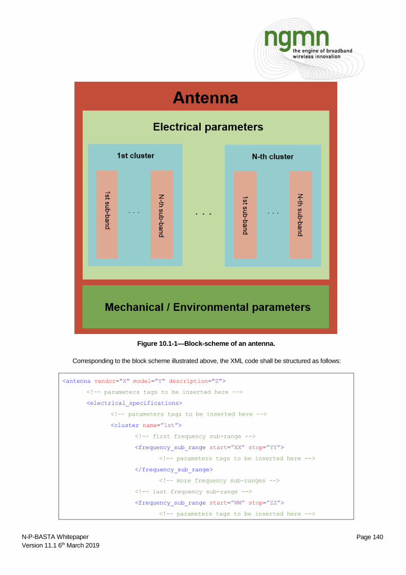
t
Page 140 N-P-BASTA Whitepaper
Version 11.1 6th March 2019
Figure 10.1-1—Block-scheme of an antenna.
Corresponding to the block scheme illustrated above, the XML code shall be structured as follows:
<antenna vendor="X" model="Y" description="Z">
<!-- parameters tags to be inserted here -->
<electrical_specifications>
<!-- parameters tags to be inserted here -->
<cluster name=”1st”>
<!-- first frequency sub-range -->
<frequency_sub_range start=”XX” stop=”YY”>
<!-- parameters tags to be inserted here -->
</frequency_sub_range>
<!-- more frequency sub-ranges -->
<!-- last frequency sub-range -->
<frequency_sub_range start=”WW” stop=”ZZ”>
<!-- parameters tags to be inserted here -->
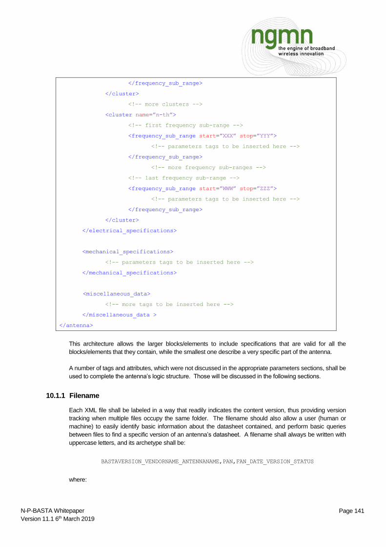
t
Page 141 N-P-BASTA Whitepaper
Version 11.1 6th March 2019
</frequency_sub_range>
</cluster>
<!-- more clusters -->
<cluster name=”n-th”>
<!-- first frequency sub-range -->
<frequency_sub_range start=”XXX” stop=”YYY”>
<!-- parameters tags to be inserted here -->
</frequency_sub_range>
<!-- more frequency sub-ranges -->
<!-- last frequency sub-range -->
<frequency_sub_range start=”WWW” stop=”ZZZ”>
<!-- parameters tags to be inserted here -->
</frequency_sub_range>
</cluster>
</electrical_specifications>
<mechanical_specifications>
<!-- parameters tags to be inserted here -->
</mechanical_specifications>
<miscellaneous_data>
<!-- more tags to be inserted here -->
</miscellaneous_data >
</antenna>
This architecture allows the larger blocks/elements to include specifications that are valid for all the
blocks/elements that they contain, while the smallest one describe a very specific part of the antenna.
A number of tags and attributes, which were not discussed in the appropriate parameters sections, shall be
used to complete the antenna’s logic structure. Those will be discussed in the following sections.
10.1.1 Filename
Each XML file shall be labeled in a way that readily indicates the content version, thus providing version
tracking when multiple files occupy the same folder. The filename should also allow a user (human or
machine) to easily identify basic information about the datasheet contained, and perform basic queries
between files to find a specific version of an antenna’s datasheet. A filename shall always be written with
uppercase letters, and its archetype shall be:
BASTAVERSION_VENDORNAME_ANTENNANAME,PAN,FAN_DATE_VERSION_STATUS
where:

t
Page 142 N-P-BASTA Whitepaper
Version 11.1 6th March 2019
BASTAVERSION is the version of the NGMN-P-BASTA whitepaper that has been used to create the
XML file. The symbol of full stop (“.”) in the version string shall be replaced with the symbol of minus
(“-”).
VENDORNAME is the name of the antenna’s vendor.
ANTENNANAME is the name of the antenna model.
PAN is the combination of the string “PAN” and the value in degrees of a specific antenna pan angle
(see Section 3.3.16). This value shall be identified by a letter indicating the sign (“P” for “plus” and “M”
for “minus”) and three figures, which shall vary between “000” and “359”. “000” shall always be
preceded by “P”. Moreover if an antenna has no pan capability, PAN shall be an empty string, and the
comma before it shall be deleted.
FAN is the combination of the string “FAN” and the value in degrees of a specific antenna fan angle
(see Section 3.3.17). This value shall be identified by three figures, which shall vary between “001”
and “360”. Moreover if an antenna has no fan capability, FAN shall be an empty string, and the
comma before it shall be deleted.
DATE is the date in which the datasheet inside the file was created. The format to use shall be
YYYY-MM-DD (four numbers for the year, two for the month and two for the day).
VERSION is written with a “V” letter and followed by two numbers. It represents the version of the
datasheet contained in the file. The first version shall always be the “00”. Along with DATE, ensures
that there can be a maximum of 100 datasheets of the same antenna created in one day.
STATUS shall describe the datasheet status. Only two values of it shall be possible: F (for “final”) and
P (for “preliminary”).
The extension of the file shall be “.xml”
An example of filename of an antenna capable of panning and fanning:
BASTA10-0_RFS_APXV99LL20BI-U,PANM150,FAN010_1999-12-30_V00_F.xml
An example of filename of an antenna not capable of panning and fanning:
BASTA10-0_RFS_APXV88LL25BI-U_2000-08-12_V10_F.xml
10.1.2 Preamble
The preamble is a part of code that was not mentioned before. It is nevertheless worth to dedicate a section
to it due to the fact that it completes the code with useful informations. It contains only two tags:
XML version and encoding:
<?xml version="1.0" encoding="UTF-8"?>
This is defined by the XML format. For information concerning this tag, it is recommended to refer to the
appropriate documentation on the web.
BASTA and its version:
<basta version="9.0.1">
The basta tag opens the datasheet, and its first attribute version points to the version of the NGMN-P-
BASTA whitepaper that has been used to create the XML file. The value associated to it shall be a string
containing the version number, which shall be the same one used to generate the filename (see Section
10.1.1).

t
Page 143 N-P-BASTA Whitepaper
Version 11.1 6th March 2019
A tag dedicated to annotations belongs to the basta tag too:
<annotation>here you can write what you want</annotation>
10.1.3 Antenna
The antenna element is the largest block and contains informations that characterize/are valid for the whole
antenna:
Antenna name, brand and description:
<antenna vendor ="huawei" model="atr4517r1" description="dxxx-790-960/1710-
2690/1710-2690-65/65/65-15i/17.5i/17.5i-m/m/m-r">
All the three attributes contain a string that describes respectively the antenna’s vendor, the antenna model
and a brief description of the antenna itself. vendor and model shall coincide respectively with
VENDORNAME and ANTENNANAME in the filename (see Section 10.1.1). This redundancy has been
added to avoid mistakes during XML files renaming. Files whose name and antenna tag don’t coincide
should not be used.
Datasheet replacement:
<replacement_datasheet datasheet="BASTA9-6_COMMSCOPE_SBNHH-1D65B,FAN065_2001-01-
01_V10_P"/>
replacement_datasheet is an optional tag that shall appear as an element inside antenna when the
datasheet contained in the file replaces a previous version of itself. An antenna replacing an older model
typically changes instead its name, therefore its datasheet shall not be taken as a substitute to an older one,
but as a brand-new datasheet. The value of datasheet shall be a string equal to the name of the replaced
datasheet without the “.xml” extension. Notice that the value of datasheet is written with uppercase letters.
10.1.4 Electrical Specifications
The electrical specifications block is the only element containing antennas’ parameters concerning
its radiation pattern and electrical features. It contains every cluster block and two other elements that have
no child tags:
Maximum power for the whole antenna:
<maximum_effective_power_antenna value="1200"/>
This tag is basically self-explanatory. Its value attribute shall be a positive integer number.
10.1.5 Cluster
Inside a cluster block there are all the parameters that belong to the specific section of the antenna
connected to a number of ports (typically two). A cluster is, in fact, defined by more tags, which contain its
core informations: name, ports and supported frequencies.
Cluster name:
<cluster name="r1"/>
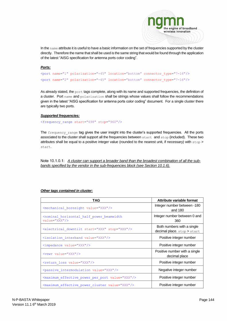
t
Page 144 N-P-BASTA Whitepaper
Version 11.1 6th March 2019
In the name attribute it is useful to have a basic information on the set of frequencies supported by the cluster
directly. Therefore the name that shall be used is the same string that would be found through the application
of the latest “AISG specification for antenna ports color coding”.
Ports:
<port name="1" polarization="+45" location=”bottom” connector_type="7-16"/>
<port name="2" polarization="-45" location=”bottom” connector_type="7-16"/>
As already stated, the port tags complete, along with its name and supported frequencies, the definition of
a cluster. Port name and polarization shall be strings whose values shall follow the recommendations
given in the latest “AISG specification for antenna ports color coding” document. For a single cluster there
are typically two ports.
Supported frequencies:
<frequency_range start="698" stop="960"/>
The frequency_range tag gives the user insight into the cluster’s supported frequencies. All the ports
associated to the cluster shall support all the frequencies between start and stop (included). These two
attributes shall be equal to a positive integer value (rounded to the nearest unit, if necessary) with stop >
start.
A cluster can support a broader band than the broadest combination of all the sub-
bands specified by the vendor in the sub-frequencies block (see Section 10.1.6).
Other tags contained in cluster:
TAG Attribute variable format
<mechanical_boresight value="XXX"/> Integer number between -180
and 180
<nominal_horizontal_half_power_beamwidth
value="XXX"/>
Integer number between 0 and
360
<electrical_downtilt start="XXX" stop="XXX"/> Both numbers with a single
decimal place. stop > start
<isolation_interband value="XXX"/> Positive integer number
<impedance value="XXX"/> Positive integer number
<vswr value="XXX"/> Positive number with a single
decimal place
<return_loss value="XXX"/> Positive integer number
<passive_intermodulation value="XXX"/> Negative integer number
<maximum_effective_power_per_port value="XXX"/> Positive integer number
<maximum_effective_power_cluster value="XXX"/> Positive integer number

t
Page 145 N-P-BASTA Whitepaper
Version 11.1 6th March 2019
10.1.6 Sub-Band
A frequency sub-band block is a section of a cluster that characterizes only a part of its whole supported
spectrum. It is the smallest logical block but also the most specific, also because it contains the highest
number of parameters. A sub-band block has no name and is uniquely defined by its frequency range.
Sub-Band:
<frequency_sub_range start="698" stop="806"/>
All the parameters included in frequency_sub_range shall only be associated to the specified frequency
range between start and stop (included). These two attributes shall be equal to a positive integer value
(rounded to the nearest unit, if necessary) with stop > start. start cannot be lower than the cluster’s
frequency_range start; similarly, stop cannot be higher than the cluster’s frequency_range stop.
All tags contained in sub-band:
TAG Attribute variable format
<gain_at_tilt min="XXX" mid="XXX" max="XXX"/> All positive numbers with a
single decimal place
<gain_over_all_tilts value="XXX" tolerance="XXX"/> Both positive numbers with
a single decimal place
<azimuth_interference_ratio value="XXX" tolerance="XXX"/> Both positive numbers with
a single decimal place
<azimuth_beamwidth value="XXX" tolerance="XXX"/> Both positive numbers with
a single decimal place
<azimuth_beam_squint value="XXX" tolerance="XXX"/> Both positive numbers with
a single decimal place
<azimuth_beam_port_to_port_tracking value="XXX"/> Positive number with a
single decimal place
<azimuth_beam_hv_tracking value="XXX"/> Positive number with a
single decimal place
<azimuth_beam_roll_off value="XXX" tolerance="XXX"/> Both positive numbers with
a single decimal place
<elevation_beamwidth value="XXX" tolerance="XXX"/> Both positive numbers with
a single decimal place
<elevation_downtilt_deviation value="XXX"/> Positive number with a
single decimal place
<front_to_back_ratio_total_power_pm30 value="XXX"/> Positive number with a
single decimal place
<front_to_back_ratio_over_30_angular_region_total_power_az
_and_el value="XXX"/>
Positive number with a
single decimal place
<null_fill value="XXX"/> Positive number with a
single decimal place
<upper_sidelobe_suppression_first value="XXX"/> Positive number with a
single decimal place
<upper_sidelobe_suppression_peak_to_20 value="XXX"/> Positive number with a
single decimal place
<upper_sidelobe_suppression_horizon_to_20 value="XXX"/> Positive number with a
single decimal place

t
Page 146 N-P-BASTA Whitepaper
Version 11.1 6th March 2019
<upper_sidelobe_suppression_maximum_level value="XXX"/> Positive number with a
single decimal place
<cross_polar_discrimination_over_sector value="XXX"/> Positive number with a
single decimal place
<cross_polar_discrimination_at_mechanical_boresight
value="XXX"/>
Positive number with a
single decimal place
<cross_polar_discrimination_over_3_db_azimuth_beamwidth
value="XXX"/>
Positive number with a
single decimal place
<cross_polar_discrimination_over_10_db_azimuth_beamwidth
value="XXX"/>
Positive number with a
single decimal place
<cross_polar_discrimination_over_3_db_elevation_beamwidth
value="XXX"/>
Positive number with a
single decimal place
<cross_polar_discrimination_over_10_db_elevation_beamwidth
value="XXX"/>
Positive number with a
single decimal place
<isolation_cross_polar value="XXX"/> Positive number with a
single decimal place
11 Note: Tolerances are intended as plus or minus (±).
11.1.1 Mechanical and Environmental Specifications
The mechanical and environmental block encompasses, under the mechanical_specifications tag,
the following elements:
TAG Attribute variable format
<dimensions height="XXX" width="XXX" depth="XXX"
reference="XXX"/>
All positive integer numbers
except reference that is an
optional string enumeration.
<packing_size height="XXX" width="XXX" depth="XXX"/> All positive integer numbers
<net_weight wo_mtg_hardware="XXX" only_mtg_hardware
="XXX"/>
Both positive numbers with a
single decimal place
<shipping_weight value="XXX"/> Positive number with a single
decimal place
<survival_wind_speed value="XXX"/> Positive integer number
<radome_material value="XXX"/> String
<radome_color value="XXX"/> String
<lightning_protection value="XXX"/> Boolean
<mechanical_distance_between_mounting_points_antenna
value="XXX"/>
Positive integer number >
antenna_dimensions height
There is also a variable number of environmental specifications included in the same element (see Section
5.11). Below an example:
TAG Attribute variable format
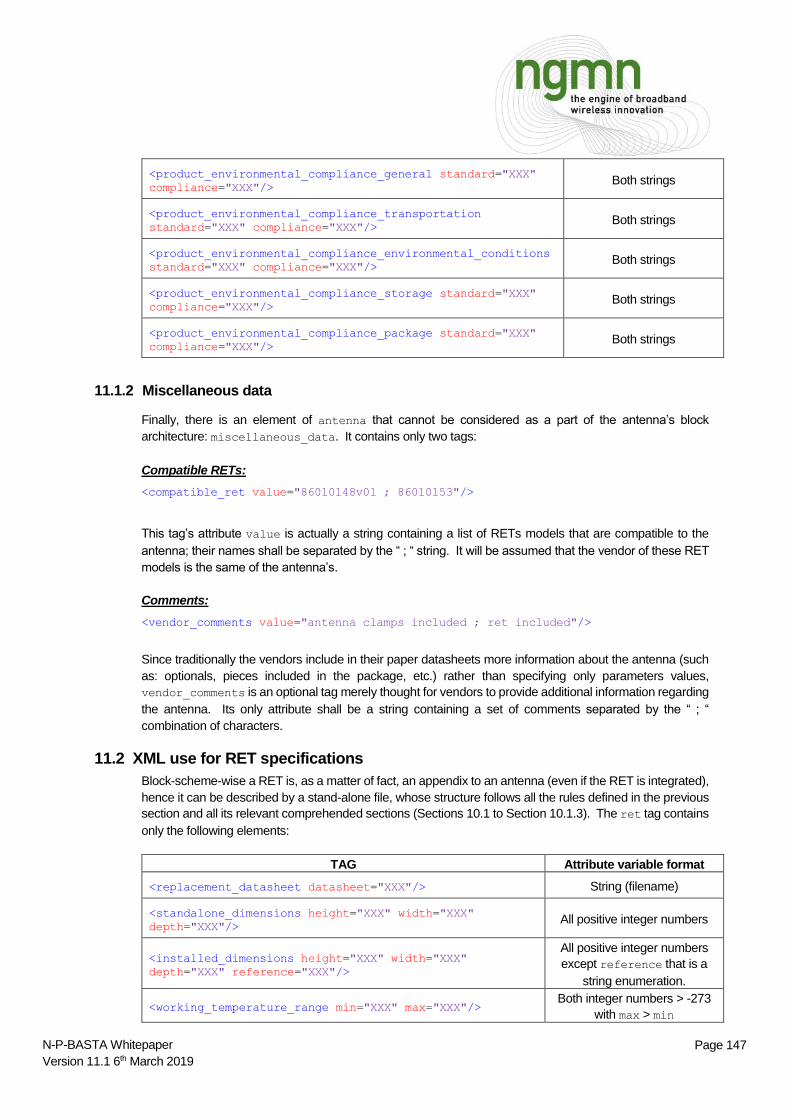
t
Page 147 N-P-BASTA Whitepaper
Version 11.1 6th March 2019
<product_environmental_compliance_general standard="XXX"
compliance="XXX"/> Both strings
<product_environmental_compliance_transportation
standard="XXX" compliance="XXX"/> Both strings
<product_environmental_compliance_environmental_conditions
standard="XXX" compliance="XXX"/> Both strings
<product_environmental_compliance_storage standard="XXX"
compliance="XXX"/> Both strings
<product_environmental_compliance_package standard="XXX"
compliance="XXX"/> Both strings
11.1.2 Miscellaneous data
Finally, there is an element of antenna that cannot be considered as a part of the antenna’s block
architecture: miscellaneous_data. It contains only two tags:
Compatible RETs:
<compatible_ret value="86010148v01 ; 86010153"/>
This tag’s attribute value is actually a string containing a list of RETs models that are compatible to the
antenna; their names shall be separated by the “ ; “ string. It will be assumed that the vendor of these RET
models is the same of the antenna’s.
Comments:
<vendor_comments value="antenna clamps included ; ret included"/>
Since traditionally the vendors include in their paper datasheets more information about the antenna (such
as: optionals, pieces included in the package, etc.) rather than specifying only parameters values,
vendor_comments is an optional tag merely thought for vendors to provide additional information regarding
the antenna. Its only attribute shall be a string containing a set of comments separated by the “ ; “
combination of characters.
11.2 XML use for RET specifications
Block-scheme-wise a RET is, as a matter of fact, an appendix to an antenna (even if the RET is integrated),
hence it can be described by a stand-alone file, whose structure follows all the rules defined in the previous
section and all its relevant comprehended sections (Sections 10.1 to Section 10.1.3). The ret tag contains
only the following elements:
TAG Attribute variable format
<replacement_datasheet datasheet="XXX"/> String (filename)
<standalone_dimensions height="XXX" width="XXX"
depth="XXX"/> All positive integer numbers
<installed_dimensions height="XXX" width="XXX"
depth="XXX" reference="XXX"/>
All positive integer numbers
except reference that is a
string enumeration.
<working_temperature_range min="XXX" max="XXX"/> Both integer numbers > -273
with max > min

t
Page 148 N-P-BASTA Whitepaper
Version 11.1 6th March 2019
<power_consumption low_power="XXX" high_power="XXX"/>
Both positive numbers with a
single decimal place and
high_power > low_power
<lose_position_on_power_failure value="XXX"/> Boolean
<compatible_standards value="XXX ; YYY ; ZZZ"/> String
<compatible_protocols value="XXX ; YYY ; ZZZ"/> String
<configuration_management value="XXX"/> String Enumeration
<antenna_configuration_available value="XXX"/> Boolean
<antenna_configuration_upgradable value="XXX"/> String Enumeration
<software_upgradable value="XXX"/> String Enumeration
<field_replacement_allowed value="XXX"/> String Enumeration
<visual_indicator_available_on_tilt_change value="XXX"/> Boolean
<daisy_chain_available value="XXX"/> Boolean

t
Page 149 N-P-BASTA Whitepaper
Version 11.1 6th March 2019
APPENDIX A – EXAMPLE OF ANTENNA DATASHEET
This is an example of single-beam antenna, whose datasheet replaces the older one. In this example the
cluster “R1” has a required parameter not applicable. All the data in the following examples is fictional.
NGMN P-Basta-Version
Vendor Name
Antenna Name
Date
Version
Status
Antenna Description
Electrical Specification
Cluster Name
Port Name P1 P2 P3 P4 P5 P6
Polarization +45 -45 +45 -45 +45 -45
Impedance Ohms 50 50 50 50 50 50
Electrical Downtilt deg 2 To 15 2 To 15 2 To 12 2 To 12 2 To 12 2 To 12
Maximum Effective Power per Port Watts 300 300 300 300 300 300
Passive Intermodulation dBc < -153 -153 -153 -153 -153 -153
Mechanical Boresight Deg 0 0 0 0 0 0
VSWR < 1.5 1.5 1.5 1.5 1.5 1.5
Return Loss dB > -14 -14 -14 -14 -14 -14
Intra-Cluster Isolation dB > 30 30 30 30 30 30
Inter-Cluster Isolation dB >
Frequency Range MHz Start-Stop
Frequency Sub-Range MHz Start-Stop 694 - 790 790 - 860 790 - 960 1710 - 1880 1850 - 1990 1920 - 2170 2500 - 2690 1710 - 1880 1850 - 1990 1920 - 2170 2500 - 2690
Min Tilt 13.5 13.5 13.5 16.5 16.5 16.5 16.5 16.5 16.5 16.5 16.5
Mid Tilt 13.6 13.6 13.6 16.6 16.6 16.6 16.6 16.6 16.6 16.6 16.6
Max Tilt 13.7 13.7 13.7 16.7 16.7 16.7 16.7 16.7 16.7 16.7 16.7
Over all Tilt 13.6 +/- 0.5 13.6 +/- 0.5 13.6 +/- 0.5 16.6 +/- 0.5 16.6 +/- 0.5 16.6 +/- 0.5 16.6 +/- 0.5 16.6 +/- 0.5 16.6 +/- 0.5 16.6 +/- 0.5 16.6 +/- 0.5
Azimuth Beamwidth deg <> 65 +/- 5 65 +/- 5 65 +/- 5 65 +/- 5 65 +/- 5 65 +/- 5 65 +/- 5 65 +/- 5 65 +/- 5 65 +/- 5 65 +/- 5
Cross Polar Discrimination at Boresight dB > 20 20 20 20 20 20 20 20 20 20 20
Cross Polar Discrimination over Sector dB > 10 10 10 10 10 10 10 10 10 10 10
Cross Polar Discrimination over 3dB Azimuth Beamwidth dB > 15 15 15 15 15 15 15 15 15 15 15
Cross Polar Discrimination over 10dB Azimuth Beamwidth dB > 10 10 10 10 10 10 10 10 10 10 10
Azimuth Beam Squint (3dB) deg <> 0 +/- 1 0 +/- 1 0 +/- 1 0 +/- 1 0 +/- 1 0 +/- 1 0 +/- 1 0 +/- 1 0 +/- 1 0 +/- 1 0 +/- 1
Azimuth Port-to-Port Tracking dB < 1 1 1 1 1 1 1 1 1 1 1
Azimuth Beam Roll Off dB <> 8 +/- 0.5 8 +/- 0.5 8 +/- 0.5 8 +/- 0.5 8 +/- 0.5 8 +/- 0.5 8 +/- 0.5 8 +/- 0.5 8 +/- 0.5 8 +/- 0.5 8 +/- 0.5
Azimuth Interference Ratio dB <> 11 +/- 0.5 11 +/- 0.5 11 +/- 0.5 11 +/- 0.5 11 +/- 0.5 11 +/- 0.5 11 +/- 0.5 11 +/- 0.5 11 +/- 0.5 11 +/- 0.5 11 +/- 0.5
Front-to-back Ratio, Total Power,+/- 30deg dB > 30 30 30 30 30 30 30 30 30 30 30
Elevation Beamwidth 3dB deg <> 18 +/- 1 18 +/- 1 18 +/- 1 8.3 +/- 0.2 8 +/- 0.2 7.3 +/- 0.3 5.8 +/- 0.3 8.2 +/- 0.4 7.9 +/- 0.2 7.3 +/- 0.6 5.8 +/- 0.3
Elevation Downtilt Deviation deg < 0.1 0.1 0.1 0.1 0.1 0.1 0.1 0.1 0.1 0.1 0.1
First Upper Side Lobe Suppression dB > 18 18 18 18 18 18 18 18 18 18 18
Upper Side Lobe Suppression Peak to +20deg dB > 20 20 20 20 20 20 20 20 20 20 20
Upper SideLobe Suppression horizon to +20deg dB > 20 20 20 20 20 20 20 20 20 20 20
Maximum Upper SideLobe Level dB > 16 16 16 16 16 16 16 16 16 16 16
Null Fill dB < N/A N/A N/A 30 30 30 30 30 30 30 30
Cross Polar Discrimination over 3dB Elevation Beamwidth dB > 15 15 15 15 15 15 15 15 15 15 15
Mechanical Specifications
Antenna Dimensions (Height x Width x Depth) mm
Packing Size (Height x Width x Depth) mm
Weight without accessories kg
Weight of accesories only kg
Shipping Weight kg
Connector Type
Connector Quantity
Connector Position
Radome Material
Radome Color RAL
Mechanical Distance between Mounting Points - Antenna mm
Lightning Protection
Wind Load
Survival Wind Speed km/h
Wind Velocity km/h
Frontal N
Lateral N
Standard
Laboratory
Extrapolation
Environmental Specifications
Storage Class 1.1
Transportation Class 2.3
Environmental conditions Class 4.1E
Package Class 1.1
Compliance EN50581:2012
Miscellaneous Data
Compatible RET's
Preliminary
1500 x 280 x 85
1700 x 300 x 100
10.1
RFS
APXV XXXX
01/10/2018
1
1695 - 2700 1695 - 2700
R > 30 ; Y1 > 30
Triple Band Antenna, No real value , only for NGMN example
R Y1 Y2
Gain dBi
10
2
R > 30 ; Y2 > 30
150
500
360
ANSI/TIA-222-G or EN 1991-1-4
1250
Direct Ground
4.3-10 Female
6
Bottom
200
PVC
RAL7035
15
694 - 960
ETSI 300-019-1-1
RoHS
ACU-A20-N
ACU-A20-S
Y1 > 30 ; Y2 > 30
ETSI 300-019-1-1
ETSI 300-019-1-2
ETSI 300-019-2-4
xy, open loop tunnel z
130

t
Page 150 N-P-BASTA Whitepaper
Version 11.1 6th March 2019
APPENDIX B – EXAMPLE OF RET DATASHEET
NGMN P-Basta-Version
Vendor Name
RET Type
Datasheet Replacement
NGMN data
Height Width Depth RET instal. ref. Comments
Actuator standalone size: Height / Width / Depth mm 110 42 88 Must be 0 /0 /0 for internal RET
Actuator installed size: Height / Width / Depth mm 110 42 88 H if antenna is known
Working temperature range °C min -40 70 max
Power consumption W low 1 10 high
Loss of position on power failure True
Compatible standards
Compatible proprietary protocols N/A
Configuration management External RET, pre-configured
Antenna configuration file availability True
Antenna configuration file upgradability Yes
Software upgradability True, by base station or proprietary protocol adapter
Replaceability in field True, without removing antenna
Visual indicator available on tilt change True
Daisy chain available True
10.1
RFS
ACU-A20-S
N/A
3GPP/AISG 2.0, AISG 1.1

t
Page 151 N-P-BASTA Whitepaper
Version 11.1 6th March 2019
APPENDIX C – LOGICAL BLOCK STRUCTURE (ANTENNA+RET)

t
Page 152 N-P-BASTA Whitepaper
Version 11.1 6th March 2019
APPENDIX D – EXAMPLE OF ANTENNA XML FILE
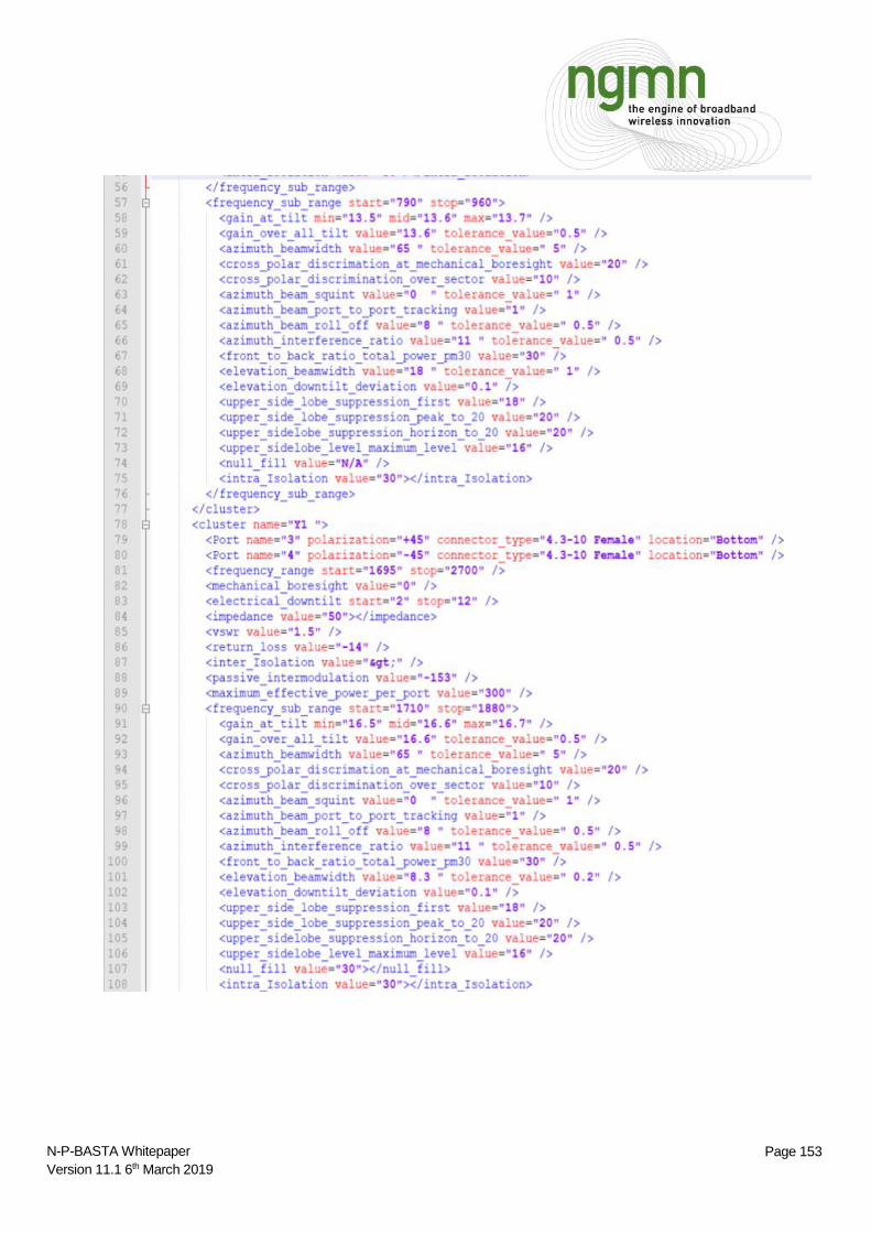
t
Page 153 N-P-BASTA Whitepaper
Version 11.1 6th March 2019

t
Page 154 N-P-BASTA Whitepaper
Version 11.1 6th March 2019
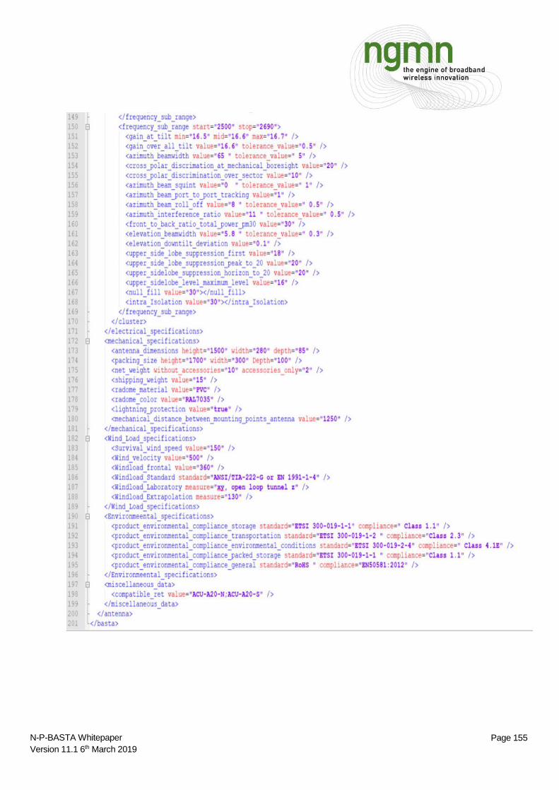
t
Page 155 N-P-BASTA Whitepaper
Version 11.1 6th March 2019
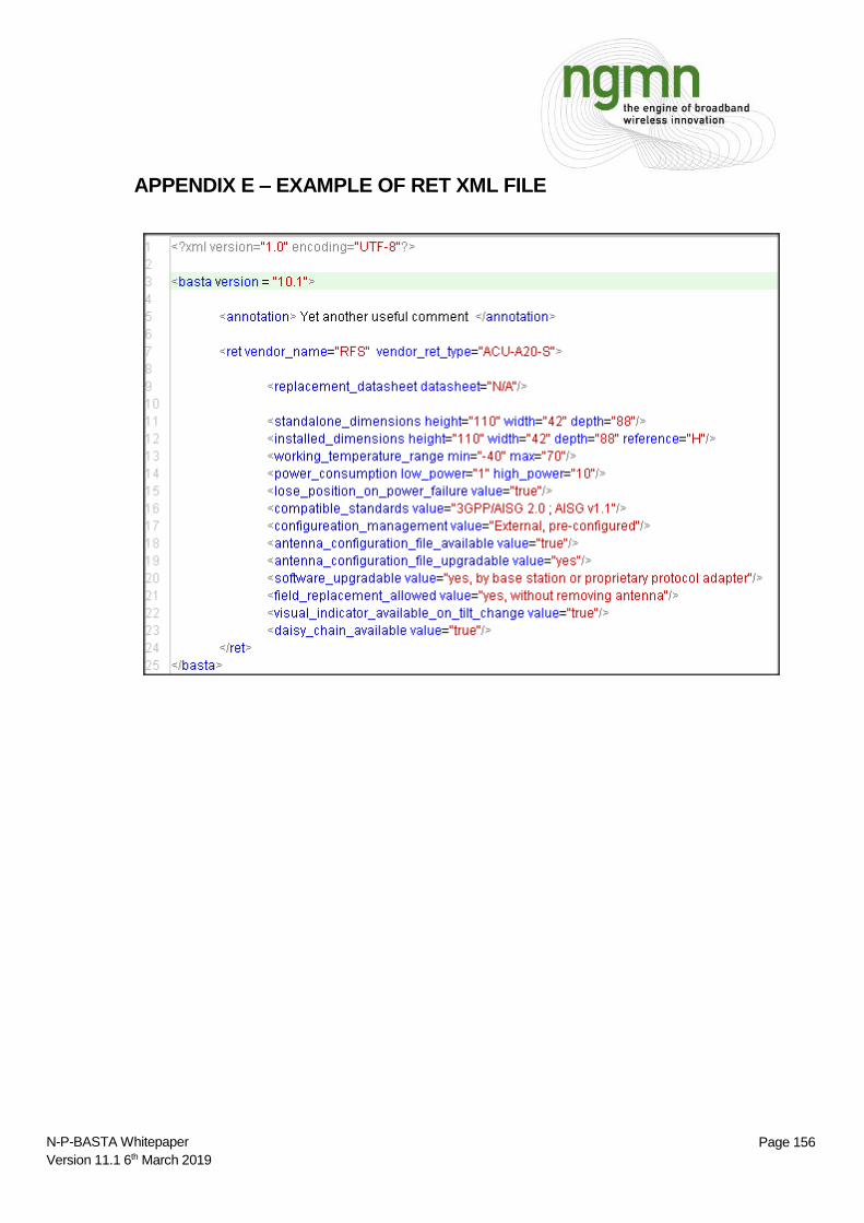
t
Page 156 N-P-BASTA Whitepaper
Version 11.1 6th March 2019
APPENDIX E – EXAMPLE OF RET XML FILE
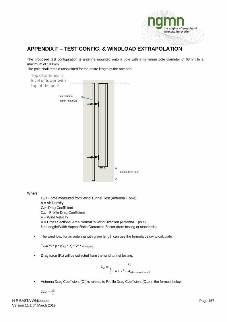
t
Page 157 N-P-BASTA Whitepaper
Version 11.1 6th March 2019
APPENDIX F – TEST CONFIG. & WINDLOAD EXTRAPOLATION
The proposed test configuration is antenna mounted onto a pole with a minimum pole diameter of 63mm to a
maximum of 100mm
The pole shall remain unshielded for the entire length of the antenna.
Where
Fw = Force measured from Wind Tunnel Test (Antenna + pole)
ρ = Air Density
Cd = Drag Coefficient
Cdp = Profile Drag Coefficient
V = Wind Velocity
A = Cross Sectional Area Normal to Wind Direction (Antenna + pole)
λ = Length/Width Aspect Ratio Correction Factor (from testing or standards)
• The wind load for an antenna with given length can use the formula below to calculate
Fw = ½ * ρ * (Cdp * λ) * V2 * AAntenna
• Drag force (Fw) will be collected from the wind tunnel testing.
𝐶𝑑 =𝐹𝑤
12
∗ 𝜌 ∗ 𝑉2 ∗ 𝐴(𝐴𝑛𝑡𝑒𝑛𝑛𝑎+𝑝𝑜𝑙𝑒)
• Antenna Drag Coefficient (Cd) is related to Profile Drag Coefficient (Cdp) in the formula below
Cdp =𝐶𝑑
𝜆
Top of antenna is level or lower with top of the pole

t
Page 158 N-P-BASTA Whitepaper
Version 11.1 6th March 2019
Frontal Wind load
Calculating the Frontal wind value (without the mast/pipe) from wind tunnel measurements
Fantenna=Fantenna + mast
×Cff
Cff=Aantenna
Aantenna+Amast_F
Cff= Calculated correction factor; frontal mast effect
Fantenna= Frontal force on the antenna alone in the frontal direction
Fantenna + mast = Frontal force on the antenna and mast in the frontal direction(test data)
Aantenna=Antenna frontal projected area
Amast_F=The exposed mast projected area
Amast_F=D×LF
D=Mast diameter
LF=Length of the exposed mast
In the absence of measured wind load on the antenna profile, the box assumption shall be used for calculating wind
load according to ANSI/TIA-222-G or EN 1991-1-4.
Calculation of the wind load:
Ffrontal = cf frontal ▪ q ▪ AF cf frontal : Frontal drag coefficient
q: dynamic pressure
AF: projected frontal area (width x length of the antenna)
EN 1991-1-4:
q = ½ ρ v2 Or q= 0.00256 V2 (lb/ft2 ) = 0.625 V2 [N/m2] ρ : air density v : wind velocity mph [m/s] cf frontal = cf,0 ∙ ψr ∙ψλ cf,0 acc. to EN 1991-1-4 Figure 1 ψr acc. to EN 1991-1-4 Figure 2 ψλ acc. to EN 1991-1-4 Figure 3 with solidity ratio ϕ =1
ANSI/TIA-222-G:
q = ½ ρ v2 Or q= 0.00256 V2 (lb/ft2 ) = 0.613 V2 [N/m2] ρ : air density v : wind velocity mph [m/s]
cf frontal : The force coefficient for flat surface can be
determined from the table number (1).
Ante
nna
Frontal Force
Wind
Direction
Fmast
LF
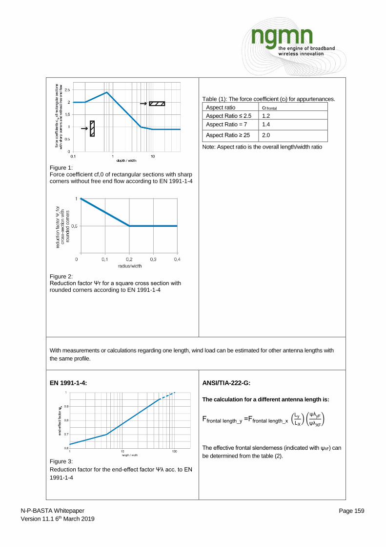
t
Page 159 N-P-BASTA Whitepaper
Version 11.1 6th March 2019
Figure 1: Force coefficient cf,0 of rectangular sections with sharp corners without free end flow according to EN 1991-1-4
Figure 2: Reduction factor Ψr for a square cross section with rounded corners according to EN 1991-1-4
Table (1): The force coefficient (cf) for appurtenances.
Aspect ratio cf frontal
Aspect Ratio ≤ 2.5 1.2
Aspect Ratio = 7 1.4
Aspect Ratio ≥ 25 2.0
Note: Aspect ratio is the overall length/width ratio
With measurements or calculations regarding one length, wind load can be estimated for other antenna lengths with
the same profile.
EN 1991-1-4:
Figure 3:
Reduction factor for the end-effect factor Ψλ acc. to EN
1991-1-4
ANSI/TIA-222-G:
The calculation for a different antenna length is:
Ffrontal length_y =Ffrontal length_x (Ly
LX) (
ψλyF
ψλXF
)
The effective frontal slenderness (indicated with ψλF) can
be determined from the table (2).

t
Page 160 N-P-BASTA Whitepaper
Version 11.1 6th March 2019
The calculation for a different antenna length is:
Ffrontal length_y =Ffrontal length_x (Ly
LX) (
ψλyF
ψλXF
)
The effective frontal slenderness (indicated with ψλF).This
factor can be determined from figure 3.
Table (2) The effective slenderness for appurtenances
Aspect ratio Effective slenderness
Aspect Ratio ≤ 2.5 0.6
Aspect Ratio = 7 0.7
Aspect Ratio ≥ 25 1.0
Notes:
Aspect ratio is the overall length/width ratio
Interpolation for values that not listed in the
table can be applied.
Where:
x: Antenna measured in wind tunnel.
y: Antenna with same cross section, but different length.
Ffrontal length_x : Frontal wind load for antenna x (measured)
Ffrontal length_y : Frontal wind load for antenna y (unknown)
Lx : Length of the antenna x.
Ly: Length of the antenna y.
ψλXF : Effective frontal slenderness for antenna x.
ψλYF: Effective frontal slenderness for antenna y.
Lx
Ante
nna X
Ly
Ante
nna Y
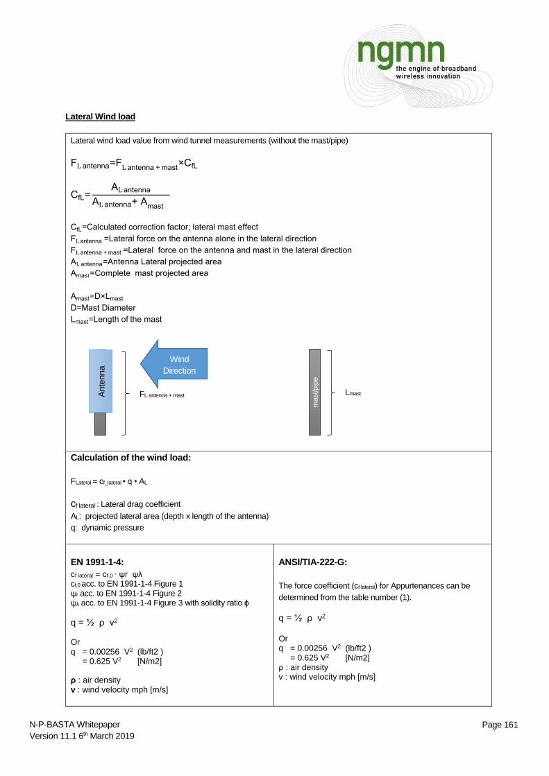
t
Page 161 N-P-BASTA Whitepaper
Version 11.1 6th March 2019
Lateral Wind load
Lateral wind load value from wind tunnel measurements (without the mast/pipe)
FL antenna=FL antenna + mast
×CfL
CfL=AL antenna
AL antenna+ Amast
CfL=Calculated correction factor; lateral mast effect
FL antenna =Lateral force on the antenna alone in the lateral direction
FL antenna + mast =Lateral force on the antenna and mast in the lateral direction
AL antenna=Antenna Lateral projected area
Amast=Complete mast projected area
Amast=D×Lmast
D=Mast Diameter
Lmast=Length of the mast
Calculation of the wind load:
FLateral = cf_lateral ▪ q ▪ AL
cf lateral : Lateral drag coefficient
AL: projected lateral area (depth x length of the antenna)
q: dynamic pressure
EN 1991-1-4:
cf lateral = cf,0 ∙ ψr ψλ cf,0 acc. to EN 1991-1-4 Figure 1 ψr acc. to EN 1991-1-4 Figure 2 ψλ acc. to EN 1991-1-4 Figure 3 with solidity ratio ϕ
q = ½ ρ v2
Or q = 0.00256 V2 (lb/ft2 ) = 0.625 V2 [N/m2] ρ : air density v : wind velocity mph [m/s]
ANSI/TIA-222-G:
The force coefficient (cf lateral) for Appurtenances can be
determined from the table number (1).
q = ½ ρ v2
Or q = 0.00256 V2 (lb/ft2 ) = 0.625 V2 [N/m2] ρ : air density v : wind velocity mph [m/s]
Ante
nna
FL antenna + mast Lmast
mast/pip
e
Wind
Direction
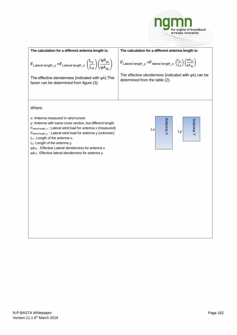
t
Page 162 N-P-BASTA Whitepaper
Version 11.1 6th March 2019
The calculation for a different antenna length is:
FLateral length_y =FLateral length_x (Ly
LX
) (ψλ
yL
ψλXL
)
The effective slenderness (indicated with ψλ).This
factor can be determined from figure (3).
The calculation for a different antenna length is:
FLateral length_y =Flateral length_x (Ly
LX) (
ψλyL
ψλXL
)
The effective slenderness (indicated with ψλ) can be
determined from the table (2).
Where:
x: Antenna measured in wind tunnel.
y: Antenna with same cross section, but different length.
Flateral length_x : Lateral wind load for antenna x (measured)
Flateral length_y : Lateral wind load for antenna y (unknown)
Lx : Length of the antenna x.
Ly: Length of the antenna y.
ψλXL : Effective Lateral slenderness for antenna x.
ψλYL: Effective lateral slenderness for antenna y.
Lx
Ante
nna X
Ly
Ante
nna Y

t
Page 163 N-P-BASTA Whitepaper
Version 11.1 6th March 2019
APPENDIX G – CHANGES FROM VERSION 9.6 TO VERSION 10.0
Figures updated and improved, new figures added.
History table replaced with changelog.
Terms definition corrected.
Whitepaper now supports omnidirectional and multi-beam antennas.
XML tag examples in each parameter’s paragraph updated.
Parameter definitions and their specification definitions corrected.
Notes added in the whole document to better specify definitions, scopes, etc.
Typos and grammar corrected.
Now the whitepaper does not contain any “must”.
Some electrical parameters added, others removed.
Some mechanical parameters removed, others included in the electrical ones.
Format of the whole whitepaper corrected.
Added thorough explanation on the calculation of all the parameters concerning sidelobes.
Added specifications on mechanical and environmental parameters.
Windload parameter deleted. Complete review will follow in next version.
Frequency points/samples recommendation completely changed.
RET specifications added.
XML chapter completely revised.
Appendices completely revised.
Overall wording generally improved.
In addition to the general changes mentioned above, the following list contains a detailed explanation of the most
important technical changes to the previous version, which exert influence to parameters’ specifications and
calculations:
Change(s)
Section(s)
interested
of v10.0
(where
applicable)
Section(s)
interested
of v9.6
(where
applicable)
Details of the change(s)
Validity 4.2 -
It is explicitly written that the validity of a new
release of the BASTA whitepaper starts from
antennas whose development begins after the
publication of the document.
Abstract Abstract Abstract The role of the whitepaper as a recommendation
for data exchange method it is now clear.
Appendix Appendix Appendix
6 documents added: example of antenna
datasheet, example of RET datasheet, logical
structure of an antenna, example of XML files for
both antenna and RET, and finally a glossary.
Purpose of document 1 1 Addressed antennas are now clearly defined as
those between 400MHz and 6000MHz.
Definitions 2; 2.7 2; 2.6
Definition of Array and Cluster added.
Now the whitepaper contains guidance on how to
generate datasheets for multi-beam and
omnidirectional antennas. This important change
t
Page 164 N-P-BASTA Whitepaper
Version 11.1 6th March 2019
is reflected throughout the document in all the
parameters’ definitions.
The definition of mechanical boresight, antenna
mounting orientation and nominal direction is
also clarified. The difference between those is
also reflected in each parameter definition.
Parameter(s) and
specifications 3.1 3.1
Included (restrictive) possibility of “n/a”
parameters.
Two important clarifications: values will be
always declared as positive unless otherwise
stated and they will be declared with a precision
of a single decimal number, unless otherwise
stated.
Ports 2.1; 3.2.2 3.2.2
Each port is associated now to a polarization, as
well as to a location and to a connector type.
Before it was possible only to specify one
location and connector type for the whole
antenna.
Ports are now compliant to AISG color coding
and naming. Arrays and clusters are
consequently compliant too. XML code is
compliant too.
Gain Ripple 3.2.4 - Definition added for non-single-beam-directional
antennas.
Elevation Squint - Removed, since it was redundant (see Elevation
Downtilt Deviation instead).
Front-to-Back ratios Multiple Multiple It is now clarified that the ratio has the maximum
and the nominal direction +/- 180° as references.
Sidelobes Multiple Multiple The value associated to the parameter may not
be a sidelobe peak.
First Upper Sidelobe
Suppression and Null Fill 4.5 3.2.14
Algorithm added to clarify how to search for the
sidelobe programmatically.
Sidelobe Suppression 20°
above Horizon and 20° above
Peak
4.5.3 -
Explanation added on how to find always a value
even if the peak of the sidelobe is not contained
in a certain region.
Cross-Polar Discrimination
(within nominal Sector, -3dB
Sector and -10dB Sector)
Multiple Multiple It is now explicitly mentioned that those are the
worst cases within their regions.
Maximum Effective Powers 3.2.19;
3.3.18 -
Added a specification for the whole antenna and
for each cluster.
Port-to-Port Isolation - 3.3.1
Removed. It was confusing, not well-defined and
generally difficult to communicate electronically.
Interband and Cross-Polar Isolation contain each
the worst cases for their definition.
Front-to-Back Ratio over 30º
Angular Region—Total Power
AZ & EL
- 3.3.2 Removed. It was not clear why it was needed.

t
Page 165 N-P-BASTA Whitepaper
Version 11.1 6th March 2019
Beam Squints Multiple Multiple It takes now explicitly as references the nominal
direction/tilt and the -3dB angular region bisect.
Specifications for special
antennas
3.3.15;
3.3.16;
3.3.17
3.3.17;
3.3.18;
3.3.19
Antennas with Pan and/or Fan abilities are now
described by one file for each degree of pan/fan.
Multi-beam antennas are now described by their
beams’ nominal directions too.
Validation and specification
of RF parameters 4 4
It is now clarified that the cuts to be taken for
azimuth and elevation shall be those containing
the maximum (peak).
It is now clarified that for the elevation pattern a
minimum of 1° spatial resolution is required for
antennas with broader main beam, and a
minimum of 0.5° for antennas with slimmer main
beam.
It is now clarified that the data shall be taken at a
minimum of 1° electrical downtilt steps and at
0.5° for the first and/or last step if the first/last tilt
is X.5°.
Statistical parameters 4.4 4.4
Definitions completely revised.
The definition of statistical “maximum” and
“minimum” are clarified: since the distribution
functions of the antenna parameters are almost
never described by a Gaussian curve, the validity
of the previous definitions of statistical
parameters is invalid:
Statistical “maximum” corresponds to the
(sometimes interpolated) value, under which
84% of the measured values lie.
Statistical “minimum” corresponds to the
(sometimes interpolated) value, over which 84%
of the measured values lie.
Consequentially the tolerance for “double-sided”
parameters was redefined too. It is now the
average between the distances from the mean
value of the figures which include 86.6% of the
measured values.
Algorithm for the calculations has been added, as
well as its explanation and a block scheme.
Examples were completely rewritten too.
Mechanical parameters 5 5
It is now written that all the mechanical
parameters are not optional if not explicitly
stated.

t
Page 166 N-P-BASTA Whitepaper
Version 11.1 6th March 2019
Antenna Dimensions 5.1 - Parameters now contain a RET reference
installation plane.
Mechanically Tilted Antennas:
Impact on Antenna Loads - 5.2
This section was out of scope, therefore
removed.
Windloads - 5.10; 5.11;
5.12; 5.13
Due to disagreement on the measurement
techniques, all the parameters concerning
antennas’ windload were removed from this
version (whitepaper scope aims to antennas
comparability).
Lightning protection 5.14 5.20
Due to impossibility to make reference to a
standard describing appropriate measurement
techniques the definition in section 5.14 was
simplified.
RET 6 -
RET’s datasheet were added as stand-alone.
An example of RET datasheet and XML code
was added to the appendices.
Frequency Spectrum 9; 9.1.3 8.1
The whitepaper is now no more limited by the
staticity of a reference to a single 3GPP
frequency table. Frequencies to be measured are
now referenced to the latest version of the
above-mentioned table.
Covers an entire algorithm explaining how to
identify frequencies to measure by keeping a
consistency with the “spectrum evolution”. Table
20 contains the result valid to the 17th of
February 2017.
The whitepaper is no more limited to the 3GPP
table but introduces the use of frequency bands
and samples for R&D purposes.
Algorithm for use of those who don’t want to work
with standard frequencies added.
XML Files 10; 10.1 9; 9.1; 9.2
WARNING: reading the whole section 10 is
strongly recommended.
Careful description of what an XML shall and
shall not contain. The following sections describe
each code block.
The entire structure of the XML was changed: it
now correctly reflects the logical structure of an
antenna.
Filename was standardized.
Appendices (reading strongly recommended)
were updated accordingly.