Reconciling Models of Diffusion and Innovation:A Theory of the Productivity Distribution and Technology Frontier∗

Jess BenhabibNYU and NBER

Jesse PerlaUBC

Christopher TonettiStanford GSB and NBER

July 10, 2017

[Download Technical Appendix]

Abstract

We study how innovation and technology diffusion interact to endogenously determine the produc-tivity distribution and generate aggregate growth. We model firms that choose to innovate, adopttechnology, or produce with their existing technology. Costly adoption creates a spread betweenthe best and worst technologies concurrently used to produce similar goods. The balance of adop-tion and innovation determines the shape of the distribution; innovation stretches the distribution,while adoption compresses it. Whether and how innovation and diffusion contribute to aggregategrowth depends on the support of the productivity distribution. With finite support, the aggregategrowth rate cannot exceed the maximum growth rate of innovators. Infinite support allows for“latent growth”: extra growth from initial conditions or auxiliary stochastic processes. While in-novation drives long-run growth, changes in the adoption process can influence growth by affectinginnovation incentives, either directly, through licensing excludable technologies, or indirectly, viathe option value of adoption.

Keywords: Endogenous Growth, Technology Diffusion, Adoption, Imitation, Innovation, Tech-nology Frontier, Productivity Distribution

JEL Codes: O14, O30, O31, O33, O40

∗An earlier version of this paper was circulated under the title “The Growth Dynamics of Innovation, Diffusion,and the Technology Frontier.” We would like to thank Philippe Aghion, Ufuk Akcigit, Paco Buera, Sebastian Di Tella,Pablo Fajgelbaum, Mildred Hager, Bart Hobijn, Hugo Hopenhayn, Chad Jones, Boyan Jovanovic, Pete Klenow, BobLucas, Erzo Luttmer, Kiminori Matsuyama, Ben Moll, Ezra Oberfield, Richard Rogerson, Tom Sargent, Nancy Stokey,Mike Waugh, and various seminar participants for useful comments and suggestions. Aref Bolandnazar and BradHackinen provided excellent research assistance. Jesse Perla gratefully acknowledges support from the University ofBritish Columbia Hampton Grant.

At any moment, there is a large gap between average and best practice technology; re-ducing this gap by disseminating the techniques used by producers at the cutting edgeof knowledge is technological progress without inventions. Any discussion of the gapbetween average and best practice techniques makes little sense unless we have somenotion of where the best practice technique came from in the first place. Without fur-ther increments in knowledge, technological diffusion and the closing of the gap betweenpractices will run into diminishing returns and eventually exhaust itself.

—Joel Mokyr, The Lever of Riches

1 IntroductionThis paper studies how the interaction between adoption and innovation determine the shape ofthe productivity distribution, the expansion of the technology frontier, and the aggregate economicgrowth rate. Empirical estimates of productivity distributions tend to have a large range, withmany low-productivity firms and few high-productivity firms within even very narrowly definedindustries and products (Syverson (2011)). The economy is filled with firms that produce similargoods using different technologies, and different firms invest in improving their technologies indifferent ways. Some firms are innovative, bettering themselves while simultaneously pushing outthe frontier by creating technologies that are new to the world. There are, however, many firmsthat purposefully choose to avoid innovating and, instead, adopt already invented ideas.

New ideas/technologies are invented and adopted frequently. For example, taking the notion ofideas-as-recipes literally, “now-ubiquitous dishes, such as molten chocolate cake or miso-glazed blackcod, did not just pop up like mushrooms after a storm. Each debuted in a specific restaurant butsoon migrated outward in slightly altered form. The putative inventors (Jean-Georges Vongerichtenin the case of molten chocolate cake, Nobu Matsuhisa for miso black cod) can claim no royalties ontheir creation.” (Raustiala and Sprigman, 2012, p.63). Miso black cod eventually diffused from theupscale Nobu in New York to the family restaurant Sakura Sushi in Whitehorse, Yukon, Canada.These examples from the restaurant industry motivate two key building blocks of our theory. First,it is useful to distinguish between innovation and adoption activity, as the economic incentives,costs, risks, abilities, and players involved in the two activities are very different. Second, there isoften a wide range of very different firms concurrently producing closely related varieties, withoutthe subsequent producer pushing the original inventor out of business due to some winner-take-allforce like creative destruction.

Although the large spread in productivity within narrowly defined industries and products,the importance of technology diffusion as a key source of growth for the less-productive, and theimportance of innovation in generating long-run growth are well established, there are few theorieswith which to study these linked phenomena. The main contribution of this paper is to develop amodel that provides tools to inspect data with these forces in mind. Crucially, the model delivers afinite, endogenously-expanding frontier with wide productivity dispersion as the result of optimalfirm behavior.

We build a model that avoids the puzzle of collapse at the frontier and the associated need forinfinite support productivity distributions, while reconciling models of innovation and idea diffusion.A finite frontier is prima facie supported by the data and turns out to be a useful and consequentialmodel feature. If the frontier were finite and constant, firms would collapse to the frontier withno long-run growth; as Mokyr points out, “without further increments in knowledge, technologicaldiffusion. . . eventually exhaust[s] itself.” To address this, previous models of idea diffusion, suchas Lucas and Moll (2014) and Perla and Tonetti (2014), have either assumed an infinite supportdistribution or some exogenous expansion of the frontier, so that there is no exhaustion of ideas. Ina sense, this phenomenon represents “latent growth”—i.e., growth that is inherent in the interplay

1

of initial conditions and exogenous stochastic processes and is foreign to the technology diffusionmechanism at the heart of the model. The implicit assumption is that some process outside ofthe model is generating an expansion of the frontier, and the model is focusing on the changein the productivity distribution generated by the diffusion process. For some purposes, such asstudying medium-run growth rates or examining the range of aggregate growth rates consistentwith exogenously given productivity distributions, this may be a very useful assumption.1 Forother purposes, such as explaining the sources of long-term growth and the role of technologydiffusion in determining growth rates, it is necessary to close the model with a joint theory ofinnovation and diffusion. Instead of using the infinite support assumption, we build such a modelof an endogenously expanding finite frontier, in which innovation and adoption occur in the long runand determine the aggregate growth rate and shape of the productivity distribution. Furthermore,we show that the finite support of the distribution has critical implications for key model propertiesconcerning latent growth, hysteresis and multiplicity and for how adoption and innovation interact.

While diffusion models typically use infinite support or exogenous innovation processes to avoidcollapse at the frontier, Schumpeterian models are designed expressly to study the endogenousexpansion of the frontier. These models of creative destruction, however, typically model the frontierand near-frontier firms, with the many low-productivity firms and associated adoption activityabsent. By combining adoption, innovation, and quality-ladder-like jumps to the frontier, our modelgenerates substantial, but bounded, productivity dispersion consistent with the firm distributiondata. Innovation pushes out the frontier and creates the technologies that will eventually beadopted, while adoption helps compress the distribution, thus keeping the laggards from fallingtoo far behind. Furthermore, innovation activity affects adoption incentives, and adoption canaffect innovation incentives. Thus, it is the interaction between these two forces that determinesthe shape of the productivity distribution and the aggregate growth rate. Since optimal adoptionand innovation behaviors generate the shape of the productivity distribution, including the spreadbetween best and worst firms, the model is well-suited to analyzing the determination of the fullproductivity distribution, not just the few firms at the frontier. Long-run growth is driven byinnovation, but that does not necessarily mean that adoption of already discovered ideas can notaffect long-run growth rates. Rather, it means that adoption affects growth rates by affecting theincentives to innovate.

Model Overview and Main Results. We first build a simple model of exogenous innovationand growth to focus on how innovation and adoption jointly affect the shape of the productivitydistribution. We then add an innovation decision in which aggregate growth is endogenously drivenin the long run by the innovation activity of high-productivity firms. At the core of the model are thecosts and benefits of adoption and innovation. Section 2.1 discusses how we model innovation andadoption and why. Firms are heterogeneous in productivity, and a firm’s technology is synonymouswith its productivity. Adoption is modeled as paying a cost to instantaneously receive a drawof a new technology. This is a model of adoption because the new productivity is drawn froma distribution related to the existing distribution of technologies currently in use for production.To represent innovation, we model firms as being in either a creative or a stagnant innovationstate; when creative, innovation generates geometric growth in productivity at a rate increasing infirm-specific innovation expenditures. A firm’s innovation state evolves according to a two-stateMarkov process, and this style of stochastic model of innovation is the key technical feature thatdelivers many of the desired model properties in a tractable framework. For example, we want theproductivity distribution to have finite support so that there are better technologies to be invented,

1In particular, these diffusion models isolate the impact of the shape of the productivity distribution on determiningthe incentives to adopt technology—which may be the dominant force in short- and medium-term growth for mostof the world.

2

in contrast to all the knowledge that will ever be known being in use for production at time zero.2At each point in time, any firm has the ability to innovate or adopt, and firms’ optimally choosewhether and how to improve their productivity. Since adoption is a function of the distribution ofavailable technologies, the productivity distribution is the aggregate state variable that moves overtime, and this movement is driven by firms’ adoption and innovation activity.

In equilibrium, there will be low-productivity firms investing in adopting technologies; stagnantfirms falling back relative to creative firms; medium-productivity creative firms investing smallamounts to grow a bit through innovation; and higher-productivity creative firms investing a lot inR&D to grow fast, create new knowledge, and push out the productivity frontier. Easy adoption, inthe sense of low cost or high likelihood of adopting a very productive technology, tends to compressthe productivity distribution, as the low-productivity firms are not left too far behind. A low costof innovation tends to spread the distribution, as the high-productivity firms can more easily escapefrom the pack. The stochastic innovation state ensures that some firms that have bad luck andstay uncreative for a stretch of time fall back relative to adopting and innovating firms, generatingnon-degenerate normalized distributions with adopting activity existing in the long run. Thus,the shape of the distribution, which typically looks like a truncated Pareto with finite support, isdetermined by the relative ease of adoption and innovation through the differing rates at whichhigh- and low-productivity firms grow.

Adoption and innovation are not two completely independent processes, with some firms per-petual adopters and some perpetual innovators. Rather, the ability of all firms to invest in bothactivities generates general equilibrium interactions between actions. The key spillover betweenadoption and innovation can be seen in the option value of adoption. For high-productivity firmswhich are far from being low-productivity adopters, the value of having the option to adopt issmall. The lower a firm’s productivity, the closer it is to being an adopter and, thus, the higherthe option value of adoption. The higher the option value of adoption, the lower is the incentive tospend on innovating to grow away from entering the adoption region. Thus, the value of adoption,which is determined by the cost of acquiring a new technology and the probability of adopting agood technology, affects incentives to innovate.

In addition to the baseline model, we introduce a sequence of extensions designed to enrich themodel to capture more ways in which innovation and adoption might interact and to relax someof the stark assumptions prevalent in the literature. We introduce a version of quality ladders byincluding a probability of leap-frogging to the frontier technology. In an extension in which tech-nologies are partially excludable and there is licensing, because adopters pay a fee to the firm whosetechnology they adopt, there is an additional direct link between adoption behavior and innovationincentives that affects the shape of the distribution and aggregate growth rates. The baseline modelhas undirected search for a new technology, in that a draw is from the unconditional distribution oftechnologies, and there is no action a firm can take to influence the source distribution. In an ex-tension, we model “directed” adoption, whereby firms can obtain a draw from a skewed distributionin which they can increase the probability of adopting better technologies at a cost. In the baselinemodel, firms exist for all time; their output and profits equal their productivity; there is no explicitcost of production; and there is a single market for the common good that all firms produce. Whilethis delivers the cleanest framework for analyzing the key forces, the model is extended to includeendogenous entry, exogenous exit, and firms that hire labor to produce a unique variety sold viamonopolistic competition to a CES final-good producer. For each extension, we examine propertiesof the BGP productivity distribution, such as the tail index and the ratio of the frontier to theminimum productivity, and whether the equilibrium is unique or if there is hysteresis in the sensethat the long-run distribution and growth rate depend on initial conditions.

2Given a continuum of firms, modeling stochastic innovation using geometric Brownian motion, as is common inthe literature, would generate infinite support instantly, while the finite-state Markov process allows for finite supportfor all time.

3

Through the baseline model and extensions, we show the types of stochastic processes that cangenerate data consistent with the empirical evidence: balanced growth with a nearly Pareto firmsize distribution in the right-tail and finite support when normalized by aggregates. We show whichfeatures are necessary to have both innovation and adoption activity exist in the long run and whenand how adoption affects the aggregate growth rate. Finally, we also show that assumptions suchas infinite initial support are not innocuous, in that the obviously counterfactual infinite supportinitial condition implies very different important model properties than the finite support initialcondition. An important distinction between BGPs with infinite and with finite support is whetherthere is latent growth—that is, the aggregate growth rate can be greater than the innovation rate,or, more starkly, whether long-run growth can exist without innovation.

While many versions of the model can be studied analytically, the endogenous growth casesmust be solved numerically. A final contribution of this paper is the development of a generallyapplicable numerical technique—based on spectral collocation and quadrature—to solve continuous-time models with heterogeneous agents that take the form of coupled Hamilton-Jacobi-Bellmanequations, Kolmogorov forward equations, and integral constraints.

Finally, since many of the results depend on the technology frontier, in Section 6, we providesome exploratory empirical analysis of the relative frontier using Compustat data. We show thatthe relative frontier, as proxied by the ratio of the 90th to the 10th percentile of the firm sizedistribution, varies significantly across industries but has been relatively stable within-industryover the past few decades.

1.1 Recent Literature

Our paper connects to the four major strands of the literature on economic growth: 1) Expand-ing ideas/varieties as exemplified by Romer (1990) and Jones (1995); 2) Schumpeterian creative-destruction, as in Aghion and Howitt (1992), Grossman and Helpman (1991), and Klette andKortum (2004); 3) Variety improvement and human capital, as in Uzawa (1961), Arrow (1962),and Lucas (1988); and 4) Technology/idea diffusion, as in Luttmer (2007), Perla and Tonetti (2014),and Lucas and Moll (2014). This section will first briefly outline the relation of our paper to themajor strands of growth theory and then will focus on a few recent papers that are most closelyrelated.

While closely linked to many of the concepts in the literature, our model is designed to addressphenomena not jointly captured by most of the existing literature: namely, within-firm produc-tivity improvement via adoption and innovation with large productivity dispersion among activelyproducing incumbents. To focus on the interaction between adoption and innovation in a simpleenvironment, we abstract from some features prominent in other models of growth. Specifically, wedevelop a one-product firm model and focus on within-firm growth. Thus, our baseline model omitsthe creation of new varieties (although we add endogenous entry in an extension), and we omitselection into exit. All of these features can be merged into one large model, but for exposition andclarity, we introduce our model of adoption and innovation in a minimalist environment withoutthese extra features.

Expanding Varieties. The expanding-varieties literature develops a theory of TFP growth bymodeling the process of discovering completely new products/ideas. The key concept in Romer(1990) is that ideas are non-rival. Thus, when combined with a production function that featuresconstant returns to scale in physical (rival) inputs, the production function has increasing returns toscale in ideas and physical inputs. Essentially, since an idea improves productivity and is non-rival,it needs to be discovered only once and can be applied without exhaustion to improve output fromthe stock of physical inputs. Because ideas are non-rival, if they could be copied by a competitorinstantly, there would be no incentive to create a new idea. Thus, excludability plays a central role

4

in determining the incentives to innovate. Given the setup in our model, there are incentives toinnovate even absent excludability since firms can coexist producing similar products, just like Nobuinventing miso black cod and many other restaurants later adopting the recipe. In an extensionin this paper, we introduce excludability in our model of innovation and adoption, bringing thisconcept, which is crucial in this literature, to the diffusion literature—capturing similar incentives,but delivering new economics via the interaction among adoption, innovation, and the shape of thedistribution.

Typically, in this literature, there are zero within-variety improvements, and all varieties aresymmetric, such that the model has no concept of heterogeneous firms. Thus, the literature is notable to speak to the wide dispersion in the firm size distribution, incumbents improving over time,or different firms undertaking different types of activities to improve productivity, such as adoptionversus innovation. Another related issue in the literature is how to model the idea productionfunction, in which the productivity of discovering new ideas is assumed to depend on the stock ofalready discovered ideas. In some sense, our model, in which the aggregate growth rate depends onthe entire productivity distribution, is a micro-foundation for the dependence of the idea productionfunction on past ideas.

Creative Destruction. Shumpeterian models tend to have a single leader producing each varietyand an inactive fringe, rather than a distribution of firms producing similar products with differentlevels of productivity. For example, in Klette and Kortum (2004) and Acemoglu, Akcigit, Bloom,and Kerr (2013), each good is produced by a single firm that may lose its exclusivity to an innovativecompetitor that creates a new leading-edge version of the product and takes over the entire productline. Crucially, all growth occurs through creative destruction rather than through innovationswithin the firm.3 See Aghion, Akcigit, and Howitt (2014) for a survey of the creative destructionliterature.

Creative destruction models are developed expressly to model the expansion of the technologyfrontier and to capture the cutthroat competitive environment associated with innovating at thefrontier. They do not, however, have a wide dispersion in firm productivity within very narrowproducts, as is apparent in the data. In this sense, our paper contains a less sophisticated model ofinnovation at the frontier, but it is well suited to model the determination of the entire productivitydistribution, not just the frontier firms. Creative destruction models cannot, however, provideguidance on the evolution of the productivity and firm size distribution for those producing wellbelow the frontier technology. In this paper, we have many lower-productivity firms, as well asseparate processes by which high- and low-productivity firms improve. That is, we can capturethe increases in productivity for the large mass of firms that do not improve through innovation,which is at the heart of the creative destruction literature. In future research, it could be fruitful tocombine a rich model of innovation at the frontier, as is typically modeled in the creative destructionliterature, with the adoption and dispersion features developed in this paper.

In some sense, one could view the quality ladder model—in which innovation for a given varietyis on top of the frontier production technology—as a form of technology diffusion. That is, theproductivity of the new leader is typically a function of the old leader’s productivity (e.g., a givenmultiplicative step size). However, even this interpretation is very different from the adoptionwe model, as it focuses on diffusion from frontier firms to new frontier firms, not firms spreadthroughout the productivity distribution that typically operate with low-productivity technologieseven post-adoption. To extend the ladder analogy to diffusion models, there may be a large numberof followers on the same ladder distributed across previously invented steps. These followers improveover time by taking modest steps up the ladder that other frontier firms built, but they rarely get

3Unlike the expanding variety models, creative destruction models generate growth via within-variety improve-ments; however, both tend to feature one firm producing each variety.

5

close to the fiercely competitive top step.

Human Capital and Variety Improvement. In contrast to the variety expansion models thatfocus on the creation of new varieties, this line of literature focuses on the creation of better ideas,either within-variety or within-individual. In our baseline model all growth comes from within-firmproductivity improvements, just as in the human capital and variety improvement literature. A keydistinction is that we model multiple ways for firms to improve their variety, via either adoptionor innovation, and study how the interaction between these two actions generates growth and theproductivity distribution. See Grossman, Helpman, Oberfield, and Sampson (2016) for a recentexample in this line of research.

Technology Diffusion. Our paper is closely related conceptually and technically to the ideadiffusion literature, including Kortum (1997), Alvarez, Buera, and Lucas (2008), Lucas (2009),Alvarez, Buera, and Lucas (2013), Perla and Tonetti (2014), and Lucas and Moll (2014). Thistechnology/idea diffusion literature focuses on how existing production technologies are distributedamong agents throughout the entire distribution and how the better technologies diffuse to low-productivity agents.4 However, the literature emphasizes neither how ideas are created in the firstplace nor the role of the technology frontier.5 Rather, these papers focus on adoption, implicitlyassuming some process that generates the ideas to be copied in the long run without explicitlymodeling that innovative behavior.6 In these models, while growth in the short or medium runcan be dominated by technology adoption, long-run growth is possible only if the productivitydistribution has infinite support with fat tails (i.e., a power-law), with a direct relationship betweenthe power-law’s tail parameter and the growth rate.7

The interaction between innovation and technology diffusion explored in this paper also ap-pears in Luttmer (2007, 2012, 2015a) and Sampson (2015), although with a different emphasisand mechanism. The main similarity with this paper is that, in all cases, diffusion is modeledas some firms drawing a new productivity from the productivity distribution of incumbents. Thebig difference is that in those papers, diffusion is generated from incumbents to new entrants, andthe equilibrium selection that the worst firms exit drives diffusion and growth. In contrast, ourpaper features incumbents adopting better technologies in equilibrium, with different implicationsfor policy counterfactuals and mapping the model to data. Another common modeling feature isthat Luttmer (2011) also features fast- and slow-growing incumbent firms—driven by differences inthe quality of blueprints for size expansion.8

Luttmer (2012, 2015a,b) provide careful analysis of the role of hysteresis and multiplicity, in-cluding the important interaction of the stochastic process with initial conditions. Luttmer (2015a)emphasizes the role of risky “experimentation,” modeled as a stochastic process distinct from deter-ministic innovation, as important in the generation of endogenous tail parameters. Our model alsohas a stochastic and deterministic component of innovation, and the risky part of innovation en-

4Some of the key empirical papers on technology diffusion examine cross-country adoption patterns, such as Cominand Hobijn (2004, 2010) and Comin, Hobijn, and Rovito (2008).

5Grassi and Imbs (2016) is a recent model of technology diffusion with a finite number of firms and, thus, a finitefrontier. The authors focus on the role of granularity in generating the measured increasingly positive correlationbetween growth and volatility as the share of large firms in a sector rises. Luttmer (2015b) also discusses the role ofa finite numbers of agents.

6Lucas and Moll (2014) provide an extension of their baseline diffusion model with the addition of exogenousinnovators in order to discuss finite support of the initial distribution.

7See the transition dynamics in Figure 2 of Perla and Tonetti (2014) for an example with a finite support pro-ductivity distribution without the creation of new ideas. In the simple calibration, growth exists for decades, drivenpurely by diffusion, before leveling off to zero growth eventually.

8In his model, firms stochastically enter the absorbing slow growth-state, whereas in this paper, firms can jumpback and forth between the states.

6

sures that there is mixing in the distribution generating adoption in the long run. Luttmer (2015b)describes a continuum of long-run growth rates that are possible in a class of diffusion models. Webuild on this, and by cleanly establishing the maximum innovation rate in the economy, we are ableto separate the long-run growth coming from the interplay of the initial conditions and stochasticprocesses. We label deviations from the intrinsic innovation rate as “latent growth”, and connectlatent growth to the hysteresis in these models generated by the infinite productivity tail (eitherdue to an initial condition or unbounded geometric random shocks). Luttmer (2015b) introducesa selection device, which is to pick the smallest growth rate (and largest tail parameter) since it isthe one that would arise from a finite support or thin-tailed initial distribution when paired withunbounded geometric random shocks to productivity. We, however, directly concentrate on therole of finiteness and its interaction with the innovation decision. Our approach also provides alens through which to understand the minimal-growth equilibrium selection device in terms of thelatent growth rate.

Recent Papers Combining Mechanisms. Our paper is most closely related in spirit to recentpapers that combine different productivity growth mechanisms in one model. Coming from thecreative destruction literature, Acemoglu and Cao (2010), Akcigit and Kerr (2016), and König,Lorenz, and Zilibotti (2016) model own-variety improvement within a Schumpeterian framework.König, Lorenz, and Zilibotti (2016) have the same structure as Klette and Kortum (2004), witha single firm using the best-practice technology to produce a variety subject to an inactive com-petitive fringe, but in which both an innovation choice in the spirit of Akcigit and Kerr (2016)and imitation of a firm’s quality from a different product-line are allowed. In this sense, it loosensthe strict separation across product lines and departs from a strictly Schumpeterian interpretationof productivity growth.9 König and Rogers (2016) combine Klette and Kortum (2004) with anexpanding variety model using collaborative networks. In each case, there is still only a singlefirm producing a given product line at any time.10 Coming from the technology diffusion litera-ture, Buera and Oberfield (2015) is a related semi-endogenous growth model of the internationaldiffusion of technology and its connection to trade in goods. The authors combine the processof idea diffusion with innovation, in the spirit of Jovanovic and Rob (1989), in which there is apositive stochastic spillover from the diffusion process itself. They model productivity upgradingaccording to one joint process that mixes innovation and adoption. In contrast, our paper modelsthese as distinct actions potentially undertaken by different firms. Furthermore, their focus is noton the endogenous determination of the shape of the distribution, since it is given exogenously bythe distribution from which innovation increments are drawn.11 The industry evolution model ofJovanovic and MacDonald (1994) has many similarities to Jovanovic and Rob (1989), but with sub-stitution between innovation and imitation and the possibility of learning-by-doing. While the firmcannot purposely target its investments in innovation vs. imitation a-priori, these activities makedifferent contributions to the growth of the firm ex-post. We build on this idea by modeling aninvestment decision in these separate productivity-enhancing activities and look at the implications

9In contrast to König, Lorenz, and Zilibotti (2016), we abstain from modeling Schumpeterian forces and keepboth the innovation and adoption technology fairly simple in order to focus on the economics of their interaction.This comes at a loss of our ability to model the richness of the innovation process for which Schumpeterian modelsexcel, but we gain tractability that enables us to better study the non-Schumpeterian forces and consider the role ofinfinite support, a finite technology frontier, and “latent growth.” A key distinction is that the finite-state Markovinnovation process that we model allows for a finite frontier, while in models with a continuum of firms on qualityladders and Poisson arrivals of multiplicative jumps, the frontier quality diverges to infinity from any initial conditionin the same way that it does for Brownian motion.

10Lashkari (2016) also models the role of innovation and technology diffusion—but emphasizes the interaction withselection in a model of creative destruction.

11Acemoglu, Aghion, Lelarge, Van Reenen, and Zilibotti (2007) also model spillovers across firms in innovation,captured by the number of firms that have attempted to implement a technology before.

7

of their interaction for long-run growth and productivity distributions.Acemoglu, Aghion, and Zilibotti (2006), Chu, Cozzi, and Galli (2014), Stokey (2014), and

Benhabib, Perla, and Tonetti (2014) also explore the relationship between innovation and diffusionfrom different perspectives. Similar to this paper, there is an advantage to backwardness in the senseof option value from the ability to adopt. The crucial element that enables the interesting trade-offbetween innovation and technology diffusion in our model is that the incumbents internalize someof the value from the evolving distribution of technologies, thus distorting their innovation choices.That is, incumbent firms not adopting today realize they may adopt in the future, and they derivepositive value from this option to adopt.12

In our extensions, we take small steps towards reconciling our model with creative destructionand expanding variety models. For example, the important role of excludability (often a precon-dition for models of variety expansion) is explored in Section 5, and leap-frogging to the frontier,which we develop in Section 3.3, is a step towards Schumpeterian forces—albeit without the crucialforce of creative destruction upon the jump.

Interpreting Productivity Dispersion and Firm Growth. Papers that closely examine pro-ductivity find a high degree of dispersion at every level of aggregation—even in narrowly definedindustries where we would expect firms to produce goods with similar characteristics.13 For ex-ample, Syverson (2011) surveys the evidence on productivity dispersion and finds that within theUS, the ratio of the top to the bottom decile is approximately 1.92:1. In places such as China andIndia, Hsieh and Klenow (2009) finds a ratio closer to 5:1.14

Absent measures of physical productivity, either revenue or firm size is commonly used to proxyfor productivity, quality, or product differentiation—which are difficult to separately identify andare typically combined into one dimension of firm profitability. As only one or two firms produceeach variety within a creative destruction model, all productivity or quality differences across firmsare interpreted as those firms having fewer product lines that are at the frontier or having frontierproducts with lower quality/productivity relative to other frontier products. The typical models donot allow the interpretation that firms are producing the same variety another firm is producing,but with below-frontier quality/productivity.

With this in mind, Garcia-Macia, Hsieh, and Klenow (2016) decompose firms’ changes in em-ployment shares as a proxy for quality into multiple possible growth channels. They find that 48percent of such changes are attributable to own-variety improvements by incumbents; 23 percentcomes from creative destruction (from both incumbents and entrants); and the expansion of vari-eties accounts for 29 percent. This confirms the important role of incumbent improvements that ishighlighted in our paper. From the perspective of our paper, however, not all such improvementsare attributed to innovation activity, as many of the firms improve via adoption.

While the stationary productivity distribution gives a sense of dispersion, the dynamics ofthe distribution give a sense of whether the creative destruction dynamics are active throughoutthe whole distribution or only for firms near the front. A classic empirical example analyzingproductivity dynamics is Baily, Hulten, Campbell, Bresnahan, and Caves (1992). In their Figure4, they show that of the all plants in the lowest (5th) quintile of the productivity distribution in1972, 54 percent were in the 4th or 5th quintile in 1982. Of those in the 1st quintile in 1972, 42percent remained in the top quintile in 1982, while only 6.5 percent exited during that period. This

12Similar to our paper, Eeckhout and Jovanovic (2002) model technological spillovers that are a function of thedistribution of firm productivity.

13More aggregated approaches, such as Acemoglu and Dell (2010) find considerable dispersion both between andwithin countries, and attribute most of it to differences in technological know-how.

14Furthermore, if productivity is partially embodied in management practices, as described in Bloom andVan Reenen (2010) and Bloom, Sadun, and Reenen (2014), then the dispersion of management practices betweenand within countries also provides strong evidence for a high degree of productivity dispersion for similar products.

8

suggests that typical changes to plants are modest in size and occur slowly (i.e., not too manychanges in leadership). Creative destruction models are designed to capture frontier firms, so itis quite possible that Schumpeterian forces are very strong inside the top quintile. This suggeststhat, although very relevant to the expansion of the frontier, creative destruction may have moremodest effects on the bottom four quintiles. See Section 6 for basic empirics of the technologyfrontier using ratios of moments in the distribution, in a sense similar to Hsieh and Klenow (2009)and Acemoglu, Aghion, Lelarge, Van Reenen, and Zilibotti (2007).

2 Baseline Model with Exogenous Stochastic InnovationWe first analyze an exogenous growth model to simplify the introduction of the environment; tofocus on the economic forces that determine the shape of the stationary normalized productivitydistribution; and to highlight that key properties of BGP equilibria depend on whether the supportof the productivity distribution is finite or infinite.

The only choice that a firm makes in this version of the model is whether to adopt a newtechnology or to continue producing with its existing technology. In Section 4, we develop anextension of this model—in which a firm chooses its innovation rate—to study how adoption andinnovation activities interact to jointly determine the shape of the productivity distribution andthe aggregate growth rate.

Throughout the paper, we present stark models in the interest of parsimony. In TechnicalAppendix G, we develop a more elaborate general equilibrium model of monopolistically competitivefirms facing CES demand that hire labor for production and productivity-improving activities tomaximize profits, with all costs denominated in units of labor at a market wage and free entrydetermining the endogenous mass of firms. Results are qualitatively equivalent, so we focus on thesimpler model for clarity of exposition.

2.1 How we Model Innovation and Adoption and Why

We model adoption and innovation as two separate methods for generating within-firm productivitygains. It could be that there is no such activity as “pure” adoption and that each act of adoptionhas the chance to create something new (as in Jovanovic and Rob (1989) and Buera and Oberfield(2015)) or requires some innovation to adapt the adopted technology to local uses. Likewise, perhapsevery act of innovation requires the concurrent adoption of some external knowledge. There is,however, a sense in which some improvements fall closer to pure innovation while others fall closerto pure adoption on the spectrum. Investments in adoption and innovation activities have differentcosts, benefits, and risks, and are done differentially by different types of firms. Thus, we believethat it is fruitful to distinguish between these activities. It is useful to model them as completelyseparate actions in order to better understand the incentives driving firms to align themselves withprimarily adoptive or primarily innovative activity and to see how these two activities interact togenerate dynamics of the productivity distribution. The key characteristic of innovation is thatit is the process that creates new knowledge. There are two essential characteristics of adoption.First, adoption does not create new knowledge but, rather, transfers existing knowledge acrossagents. Second, the opportunities available to an adopting firm necessarily depend on the existingtechnologies that are available to adopt. To make sure that we can separately capture the incentivesand effects of these two types of activities, the innovation process in our model does not share thesetwo essential properties of adoption, and the adoption process does not share this key characteristicof innovation.

To capture these features, we model adoption as a meet and copy process by which an adopterdraws a new technology with some randomness that is a function of the distribution of technologiesactively in use. This is similar to the diffusion models in Perla and Tonetti (2014) and Lucas and

9

Moll (2014). Adopters would prefer to copy the frontier technology, but due to the difficulty offinding and implementing the best technologies, they will typically end up with technology thatis better than their own but not at the frontier. Innovation is important in this paper becauseit generates an endogenously expanding productivity frontier. We model innovation as autarkicgeometric growth (as in Atkeson and Burstein (2010) and Stokey (2014)), in the sense that thereturns are only a function of the innovating firm’s productivity level and not of the productivitydistribution. This model of innovation delivers an endogenously expanding frontier in the simplestway, so that we can focus on the interaction between the distinct activities of innovation andadoption.

Since the key property of innovation is the creation of new technologies, which we capture viathe expansion of the frontier, it is essential that our model of innovation permits a productivitydistribution that has finite support for all finite times. As we will show, it turns out that a keydistinction that determines the fundamental properties of BGP equilibria is whether the long-runproductivity distribution has finite or infinite support. The important difference is between infiniteand finite support in the long run, independent of whether infinite support occurs due to initialconditions with infinite support or to an exogenous process that generates infinite support.15 Thismotivates our use of a finite-state Markov process for innovation growth rates: with this process,growth rates are always bounded for all firms over any positive time interval, and infinite supportin the stationary distribution arises only from initial conditions with infinite support.

Beyond allowing for a finite technology frontier, modeling an innovation process with a boundedmaximum growth rate (such as our finite-state Markov chain) offers an additional advantage. Sincethe process is bounded, the innovation rate in a fully-specified growth model must be less than orequal to the maximum growth rate—whether that rate is determined endogenously or exogenously.Hence, if the growth rate of the aggregate economy is greater than the maximum innovation rate—as it is in the infinite support version of our model—then the degree of “latent growth” in theeconomy is clearly defined. That is, if the aggregate growth rate is greater than the maximumidiosyncratic growth rate, there must be latent growth. With unbounded innovation rates, such asGBM or multiplicative Poisson arrivals, there is no maximum innovation rate or zero-latent-growthbenchmark for the economy, and, thus, it is difficult to determine what the sign of the latent growthmay be.

See Technical Appendix A for more discussion of the strengths, weaknesses, and failures of thisand many alternative innovation processes.

2.2 The Baseline Model

Firm Heterogeneity and Choices. A continuum of firms produce a homogeneous productand are heterogeneous over their productivity, Z, and innovation ability, i ∈ {`, h}. For sim-plicity, firm output equals firm profits equals firm productivity, Z. The mass of firms of pro-ductivity less than Z in innovation state i at time t is defined as Φi(t, Z) (i.e., an unnormal-ized CDF). Define the technology frontier as the maximum productivity of any firm, Z(t) ≡sup {support {Φ`(t, ·)} , support {Φh(t, ·)}} ≤ ∞, and normalize the mass of firms to 1 so thatΦ`(t, Z(t)) + Φh(t, Z(t)) = 1. At any point in time, the minimum of the support of the distribu-

15Infinite support can be present from the beginning due to an initial condition (e.g., Perla and Tonetti (2014),Lucas and Moll (2014)). Alternatively, infinite support can arise from an innovation process with geometric stochasticshocks generating an infinite-support power law as its stationary distribution from any initial condition (e.g., Luttmer(2007), Perla, Tonetti, and Waugh (2015) Appendix, and the GBM example in Technical Appendix E). For example,in the case of processes using Brownian Motion or a Poisson arrival of geometric jumps, even an initial conditionwith finite support immediately becomes infinite with a continuum of agents. The issue in either of those two casesis that the growth rates in any strictly positive amount of time are unbounded. The properties of the equilibria arelargely the same if the infinite support comes from geometric stochastic shocks or initial conditions, as is seen in thenested solution of Perla, Tonetti, and Waugh (2015).

10

tion will be an endogenously determined Mi(t), so that Φi(t,Mi(t)) = 0. Define the distributionunconditional on type as Φ(t, Z) ≡ Φ`(t, Z) + Φh(t, Z).

A firm with productivity Z can choose to continue producing with its existing technology, inwhich case it would grow stochastically according to the exogenous innovation process, or it canchoose to adopt a new technology.

Stochastic Process for Innovation. In the high innovation ability state (h), a firm is innovatingand its productivity is growing at a deterministic rate γ.16 In the low innovation ability state (`), ithas zero productivity growth from innovation (without loss of generality).17 Sometimes, firms havegood ideas or projects that generate growth, and sometimes firms are just producing using theirexisting technology. Innovation ability evolves according to a continuous-time two-state Markovprocess that drives the exogenous growth rate of an operating firm. This process allows for stochas-tic innovation with a finite frontier and will permit equilibria in which adoption persists in the longrun and growth is driven by the innovation choices of frontier firms. See Technical Appendix A fora discussion of the strengths, weaknesses, and failures of this and many alternative innovation pro-cesses (e.g., Poisson arrival of jumps or drifts; IID growth rates and singular perturbation methods;reflected geometric Brownian motion (GBM); deterministic heterogeneous growth rates, etc.). Theinnovation states are modeled primarily for technical reasons related to continuous-time, combinedwith the desire to model stochastic innovation and finite-support distributions, rather than beingof first order interest per se. In some loose sense, with high switching rates this process is quan-titatively similar to IID growth rate shocks without the associated continuous-time measurabilityissues.

The jump intensity from low to high is λ` > 0 and from high to low is λh > 0. Since the Markovchain has no absorbing states, and there is a strictly positive flow between the states for all Z, thesupport of the distribution conditional on ` or h is the same (except, perhaps, exactly at an initialcondition). Recall that support {Φ(t, ·)} ≡ [M(t), Z(t)). The growth rate of the upper and lowerbounds of the support are defined as g(t) ≡M ′(t)/M(t) and gZ(t) ≡ Z ′(t)/Z(t) if Z(t) <∞.

For notational simplicity, define the differential operator ∂ such that ∂z ≡ ∂∂z and ∂zz ≡ ∂2

∂z2 .When a function is univariate, derivatives will be denoted as M ′(z) ≡ ∂zM(z) ≡ dM(z)

dz .

Adoption and Technology Diffusion. A firm has the option to adopt a new technology bypaying a cost. Adoption means switching production practice by changing to a technology thatsome other firm is using. We model this adoption process as undirected search across firms.18 Thatis, when a firm chooses to adopt, it immediately switches its productivity to a draw from a functionof the existing productivity distribution Φi(t, Z).19 Assume that an adopting firm draws an (i, Z)from distributions Φ`(t, Z) and Φh(t, Z), where Φi(t, Z) is the probability that an adopting firmbecomes type i and has productivity less than Z. Let Φi be such that Φ`(t, 0) = Φh(t, 0) = 0 andΦ`(t, Z(t)) + Φh(t, Z(t)) = 1. Φi will be determined by the equilibrium Φ`(t, Z) and Φh(t, Z). Theexact specification of Φi(t, Z) typically does not affect the qualitative results, so we will write the

16In Section 4, the growth rate γ will become a control variable for a firm, with the choice subject to a convex cost.17The different innovation types are akin to Acemoglu, Akcigit, Bloom, and Kerr (2013)—albeit without the

selection of entry inherent in that model.18Instead of random matching, Luttmer (2015a) uses matching of teachers and students. The sorts of learning delays

embedded in Luttmer (2015a,b) give a qualitatively similar foundation to random matching from some distortion ofthe productivity distribution. Furthermore, If the discrete choice of an immediate innovation arrival seems stark, analternative is to use choice of an innovation intensity, as in Lucas and Moll (2014). Since the optimal innovationintensity is decreasing in relative productivity in that model, it would deliver qualitatively similar results at theaggregate level.

19See Technical Appendix C.2 for a proof showing that a firm’s ability to recall its last productivity doesn’t changethe equilibrium conditions; and Technical Appendix C.1 for a derivation when adoption is not instantaneous—whereour main specification is the limit of the adoption arrival rate going to infinity.

11

process fairly generally and then analyze specific cases. One simplification that we maintain is thatthe draw of a new (i, Z) is independent of a firm’s current type. A version of the model in whichthe firm can direct its search towards better technologies at some cost is nested in Section 5.

The cost of adoption grows as the economy grows. The endogenous scale of the economy issummarized by the minimum of support of the productivity distribution M(t). For simplicity, thecost of adoption is proportional to the scale of the aggregate economy: ζM(t).

Firm Value Functions. Firms discount at rate r > 0. Let Vi(t, Z) be the continuation valuefunctions—i.e., the value at time t of being an i-type firm and producing with productivity Z.

rV`(t, Z) = Z + λ` (Vh(t, Z)− V`(t, Z))︸ ︷︷ ︸Jump to h

+ ∂tV`(t, Z)︸ ︷︷ ︸Capital Gains

(1)

rVh(t, Z) = Z + γZ∂ZVh(t, Z)︸ ︷︷ ︸Exogenous Innovation

+λh (V`(t, Z)− Vh(t, Z))︸ ︷︷ ︸Jump to `

+∂tVh(t, Z). (2)

A firm’s continuation value derives from instantaneous production plus capital gains as wellas productivity growth if in the high innovation ability state, and it accounts for the intensity ofjumps between innovation abilities i.

The value of adopting is the continuation value of having a new productivity and innovationtype drawn from Φ` and Φh minus the cost of adoption:

Net Value of Adoption =∫ Z(t)

M(t)V`(t, Z)dΦ`(t, Z) +

∫ Z(t)

M(t)Vh(t, Z)dΦh(t, Z)︸ ︷︷ ︸

Gross Adoption Value

− ζM(t)︸ ︷︷ ︸Adoption Cost

. (3)

Optimal Adoption Policy and the Minimum of the Productivity Distribution Support.Since the value of continuing is increasing in Z, and the net value of adopting is independent ofZ, the firm’s optimal adoption policy takes the form of a reservation productivity rule. All firmschoose an identical threshold, Ma(t), above which they will continue operating with their existingtechnology and, otherwise, will adopt a new technology (i.e., a firm with Z ≤ Ma(t) is in theadoption region of the productivity space). While the adoption threshold could depend on the typei, see Appendix A.2 for a proof showing that ` and h firms choose the same threshold, Ma(t), ifthe net value of adoption is independent of the current innovation type.

As draws are instantaneous, for any t > 0, this endogenous Ma(t) becomes the evolving min-imum of the Φi(t, Z) distribution, M(t), and in an abuse of notation, we will refer to both theminimum of support and the firm adoption policy as M(t) going forward.20

In principle, there may be adopters of either innovation type with productivity in the commonadoption region with Z ≤M(t). Define Si(t) ≥ 0 as the flow of i-type firms entering the adoptionregion at time t. Denote the total flow of adopting firms as S(t) ≡ S`(t) + Sh(t).

The Firm Problem. A firm’s decision problem can be described as choosing an optimal stop-ping time of when to adopt. Necessary conditions for the optimal stopping problem include the

20To see why the minimum support is the endogenous threshold, consider instantaneous adoption as the limit ofthe Poisson arrival rate of draw opportunities approaching infinity. In any positive time interval, firms wishing toadopt would gain an acceptable draw with probability approaching 1, so that Z > M(t) almost surely. Because ofthe immediacy of draws, the stationary equilibrium does not depend on whether draws are from the unconditionaldistribution or from the distribution conditional on being above the current adoption threshold. This is the same asthe small time limit of Perla and Tonetti (2014), which solves both versions of the model. A more formal derivationof this cost function as the limit of the arrival rate of unconditional draws is in Technical Appendix C.1.

12

continuation value functions and, at the endogenously chosen adoption boundary, M(t), valuematching,

Vi(t,M(t))︸ ︷︷ ︸Value at Threshold

=∫ Z(t)

M(t)V`(t, Z)dΦ`(t, Z) +

∫ Z(t)

M(t)Vh(t, Z)dΦh(t, Z)︸ ︷︷ ︸

Gross Adoption Value

− ζM(t)︸ ︷︷ ︸Adoption Cost

, (4)

as well as smooth-pasting conditions,

∂ZV`(t,M(t)) = 0 if M ′(t) > 0 (5)∂ZVh(t,M(t)) = 0 if M ′(t)− γM(t) > 0. (6)

Value matching states that at the optimal adoption reservation productivity, a firm must beindifferent between producing with the reservation productivity or adopting a new productivity.Smooth-pasting is a technical requirement that can be interpreted as an intertemporal no-arbitragecondition that ensures that the recursive system of equations is equivalent to the fundamentaloptimal stopping problem. Thus, the smooth-pasting conditions are necessary only if firms at theboundary are moving backwards relative to the boundary over time.

The Technology Frontier. Given the adoption and innovation processes, if Z(0) <∞, then Z(t)will remain finite for all t, as it evolves from the innovation of firms in the interval infinitesimallyclose to Z(t); that is, Z ′(t)/Z(t) = γ if Φh(t, Z(t)) − Φh(t, Z(t) − ε) > 0, for all ε > 0. With thecontinuum of firms and the memoryless Poisson arrival of changes in i, there will always be some hfirms that have not jumped to the low state for any t, so the growth rate of the frontier is alwaysγ.

Law of Motion of the Productivity Distribution. The Kolmogorov Forward Equation (KFE)describes the evolution of the productivity distribution for productivities above the minimum ofthe support. The KFEs in CDFs for ` and h type firms are

∂tΦ`(t, Z) = −λ`Φ`(t, Z) + λhΦh(t, Z)︸ ︷︷ ︸Net Flow from Jumps

+ (S`(t) + Sh(t))︸ ︷︷ ︸Flow of Adopters

Φ`(t, Z)︸ ︷︷ ︸Draw ≤ Z

− S`(t)︸ ︷︷ ︸`-Adopters

(7)

∂tΦh(t, Z) = −γZ∂ZΦh(t, Z)︸ ︷︷ ︸Innovation

−λhΦh(t, Z) + λ`Φ`(t, Z) + (S`(t) + Sh(t))Φh(t, Z)− Sh(t). (8)

For each type i, the KFEs keep track of inflows and outflows of firms with a productivity levelbelow Z. An i-type firm with productivity less than Z stops being in the i-distribution below Z ifit keeps its type and increases its productivity above Z or if it changes its type.

A firm can keep its type and increase its Z in two ways: adoption or innovation. Because anadopting firm has probability Φi(t, Z) of becoming type i and drawing a productivity less thanZ, and there are (S`(t) + Sh(t)) number of firms adopting, (S`(t) + Sh(t))Φi(t, Z) is added tothe i-distribution. Additionally, the flow of adopters of each type, Si(t), is subtracted from thecorresponding distribution (this term appears conditional on any Z because adoption occurs atthe minimum of support). Intuitively, the adoption reservation productivity acts as an absorbingbarrier sweeping through the distribution from below. As it moves forward, it collects adoptersat the minimum of support, removes them from the distribution, and inserts them back into the

13

distribution according to Φ.21The KFE for the h-types has a term that subtracts the firms that grow above Z through

innovation: there are ∂ZΦh(t, Z) number of h-type firms at productivity Z, and because innovationis geometric, they grow above Z at rate γ.22

Firms of productivity Z switching from type i to type i′ leave the i-distribution and enter thei′-distribution at rate λi. For example, there are Φ`(t, Z) many `-type firms with productivity lessthan Z, and they leave the ` distribution at rate λ` and enter the h-distribution at the same rate.

Consumer Welfare and the Interest Rate The firms are owned by a representative consumerwho values the undifferentiated good with log utility and a discount rate ρ > 0.23 Given theproductivity distribution Φ(t, Z), welfare is

U(t) =∫ ∞

0e−ρτ log

∫ ∞M(t)

Z∂ZΦ(t+ τ, Z)dZ︸ ︷︷ ︸Aggregate Output

dτ. (14)

As is standard, along a balanced growth path with aggregate output growing at rate g, the discountrate that a firm faces is

r = ρ+ g. (15)

2.3 Normalization, Stationarity, and Balanced Growth Paths

In this paper, we study economies on balanced growth paths (BGPs), in which the distribution isstationary when properly rescaled and aggregate output grows at a constant rate. The economyis characterized by a system of equations defining the firm problem, the laws of motion of theproductivity distributions, and consistency conditions that link firm behavior and the evolution ofthe distributions. To compute BGP equilibria, it is convenient to transform this system to a set ofstationary equations. While we could normalize by any variable growing at the same rate as the

21Recognizing that the λi jumps are of measure 0 when calculating how many firms cross the boundary in anyinfinitesimal time period, the flow of adopters comes from the flux across the moving M(t) boundary.

S`(t) ≡M ′(t)∂ZΦ`(t,M(t)) (9)

Sh(t) ≡(M ′(t)− γM(t)

)︸ ︷︷ ︸Relative Speed of Boundary

∂ZΦh(t,M(t))︸ ︷︷ ︸PDF at boundary

. (10)

This is consistent with the solution to the ODEs in equations (7) and (8) at Z = M(t), as is apparent in the normalizedequations (21) and (22).

22To account for the drift component, assume a stochastic process with a drift µ(z), PDF f(t, z), and CDF F (t, z).The KFE comes from the adjoint to infinitesimal generator:

∂tf(t, z) = −∂z [µ(z)f(t, z)] + . . . (11)

Integrating to get the CDF F (t, z), either using the fundamental theorem of calculus or interchanging the order ofdifferentiation and integration, yields

∂tF (t, z) = −µ(z)f(t, z) + . . . (12)= −µ(z)∂zF (t, z) + . . . (13)

23The appendix uses a general firm discount rate r, and the numerical algorithm in Technical Appendix B is imple-mented for an arbitrary CRRA utility function. Using log utility here simplifies a few of the parameter restrictionsand expressions in the algebra compared to linear utility or general CRRA.

14

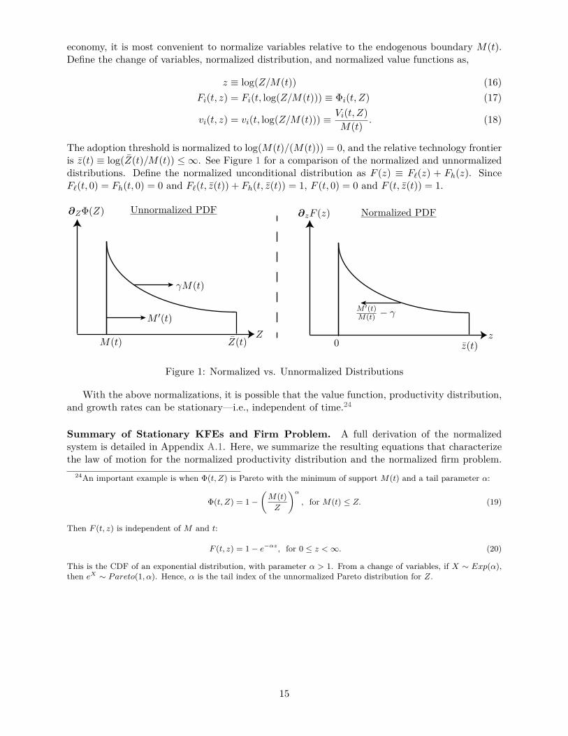
economy, it is most convenient to normalize variables relative to the endogenous boundary M(t).Define the change of variables, normalized distribution, and normalized value functions as,

z ≡ log(Z/M(t)) (16)Fi(t, z) = Fi(t, log(Z/M(t))) ≡ Φi(t, Z) (17)

vi(t, z) = vi(t, log(Z/M(t))) ≡ Vi(t, Z)M(t) . (18)

The adoption threshold is normalized to log(M(t)/(M(t))) = 0, and the relative technology frontieris z(t) ≡ log(Z(t)/M(t)) ≤ ∞. See Figure 1 for a comparison of the normalized and unnormalizeddistributions. Define the normalized unconditional distribution as F (z) ≡ F`(z) + Fh(z). SinceF`(t, 0) = Fh(t, 0) = 0 and F`(t, z(t)) + Fh(t, z(t)) = 1, F (t, 0) = 0 and F (t, z(t)) = 1.

∂ZΦ(Z)

ZM(t)

M ′(t)

γM(t)

∂zF (z)

z0

M ′(t)M(t) − γ

Unnormalized PDF Normalized PDF

Z(t) z(t)

Figure 1: Normalized vs. Unnormalized Distributions

With the above normalizations, it is possible that the value function, productivity distribution,and growth rates can be stationary—i.e., independent of time.24

Summary of Stationary KFEs and Firm Problem. A full derivation of the normalizedsystem is detailed in Appendix A.1. Here, we summarize the resulting equations that characterizethe law of motion for the normalized productivity distribution and the normalized firm problem.

24An important example is when Φ(t, Z) is Pareto with the minimum of support M(t) and a tail parameter α:

Φ(t, Z) = 1−(M(t)Z

)α, for M(t) ≤ Z. (19)

Then F (t, z) is independent of M and t:

F (t, z) = 1− e−αz, for 0 ≤ z <∞. (20)

This is the CDF of an exponential distribution, with parameter α > 1. From a change of variables, if X ∼ Exp(α),then eX ∼ Pareto(1, α). Hence, α is the tail index of the unnormalized Pareto distribution for Z.

15

The equations that determine the stationary productivity distributions are:

0 = gF ′`(z)− λ`F`(z) + λhFh(z) + (S` + Sh)F`(z)− S` (21)0 = (g − γ)F ′h(z)− λhFh(z) + λ`F`(z) + (S` + Sh)Fh(z)− Sh (22)0 = F`(0) = Fh(0) (23)1 = F`(z) + Fh(z) (24)S` = gF ′`(0), if g > 0 (25)Sh = (g − γ)F ′h(0), if g > γ. (26)

The necessary conditions of the normalized firm problem are:

ρv`(z) = ez − gv′`(z) + λ` (vh(z)− v`(z)) (27)ρvh(z) = ez − (g − γ)v′h(z) + λh (v`(z)− vh(z)) (28)

v(0) = 1ρ

=∫ z

0v`(z)dF`(z) +

∫ z

0vh(z)dFh(z)− ζ (29)

v′`(0) = 0, if g > 0 (30)v′h(0) = 0, if g > γ. (31)

Given that both firm types choose the same adoption threshold, we drop the type index for thevalue functions at the adoption threshold: v(0) ≡ vi(0).

Equations (21) to (24) are the stationary KFEs with initial conditions and boundary values.Recall that g is the growth rate of the minimum of support and γ the innovation growth rate. Inthe normalized setup, firms are moving backwards towards the constant minimum of support, andtheir growth rate determines the speed at which they are falling back. S` in equation (25) is theflow of ` agents moving backwards at a relative speed of g across the adoption barrier, while Sh inequation (26) is the flow of h agents moving backwards at the slower relative speed of g− γ acrossthe barrier. The Fi(z) specification is some function of the equilibrium Fi(z), and will be analyzedfurther in Sections 3.1 to 3.3.

Equations (27) and (28) are the Bellman Equations in the continuation region, and (29) is thevalue-matching condition between the continuation and technology adoption regions. The smooth-pasting conditions in (30) and (31) are necessary only if the firms of that particular i are driftingbackwards relative to the adoption threshold. See Figure 2 for a visualization of the normalizedBellman equations.

0 z z

vi

vi(0)

λh

λℓ

vh(z)

vℓ(z)

η

Figure 2: Normalized, Stationary Value Functions

16

Equilibrium Definitions. This paper studies balanced growth path equilibria, defined below.

Definition 1 (Recursive Competitive Equilibrium with Exogenous Innovation). A recursive com-petitive equilibrium with exogenous innovation consists of initial distributions Φi(0, z), adoptionreservation productivity functions Mi(t), value functions Vi(t, z), interest rates r(t), and sequencesof productivity distributions Φi(t, z), such that

1. given r(t) and Φi(t, z), Mi(t) are the optimal adoption reservation productivities, with Vi(t, z)the associated value functions;

2. given Mi(t) and Φi(t, z), r(t) is consistent with the consumer’s intertemporal marginal rateof substitution;

3. given Mi(t), Φi(t, z) fulfill the laws of motion in (7) and (8) subject to the initial conditionΦi(0, z).

Definition 2 (Balanced Growth Path Equilibrium with Exogenous Innovation). A balanced growthpath equilibrium with exogenous innovation is a recursive competitive equilibrium such that thegrowth rate of aggregate output is constant and the normalized productivity distributions are sta-tionary. This is equivalent to requiring that Fi(t, z) = Fi(z) and g(t) ≡M ′(t)/M(t) = g.

Define the growth rate of aggregate output as gE(t) ≡ ∂tEt [Z] /Et [Z]; then,

Lemma 1 (Growth of the Endogenous Adoption Threshold and Aggregate Output). On a balancedgrowth path, the growth rate of the endogenous threshold, M(t), must be the same as the growthrate of aggregate output. That is, g = gE.

Proof. The value-matching condition in (29) is normalized to the endogenous threshold, and, hence,adoption has a constant and strictly positive cost. Thus, as v(z) ≥ z, if the expected value of adraw from the technology distribution were not stationary relative to the adoption cost, then thevalue-matching could not hold with equality for all t. See Appendix A.7 for a similar, and moreformal, case.

How Adoption and Innovation Generate a Stationary Normalized Distribution. Aswe will show, with geometric growth, the stationary solutions will endogenously become power-law distributions asymptotically, as discussed with generality in Gabaix (2009). Figure 3 providessome intuition on how proportional growth and adoption can create a stationary distribution.Stochastic innovation spreads out the distribution and, in the absence of endogenous adoption, thiswould prevent the existence of a stationary distribution. Without endogenous adoption, there is no“absorbing" or “reflecting" barrier, and proportional random shocks generate a variance divergingto infinity. However, when adoption is endogenous, as the distribution spreads, the incentives toadopt a new technology increase, and the adoption decisions of low-productivity agents then actto compress the distribution. In a BGP equilibrium, technology diffusion can balance innovation,thus allowing for a stationary normalized distribution.

Much of the intuition for how innovation and adoption can generate a stationary normalizedpower-law productivity distribution can be seen in the same model, except with innovation thatfollows geometric Brownian motion. Technical Appendix E solves this modified model in closedform. In the GBM case, however, even with a finite Z(0) initial condition, the support of astationary F (z) will be [0,∞) since, with a continuum of agents, Brownian motion instantaneouslyincreases the support of the distribution to infinity. Thus, this GBM model is well-suited to gainingintuition for some features of our baseline model, but it is ill-suited to study the main questionssurrounding the expansion of the frontier, which drive the analysis in this paper.

17

Another advantage of our specification compared to GBM is that any firm’s maximum growthrate is bounded by the innovation rate γ. Hence, if the aggregate growth rate g > γ, then wecan easily identify conditions under which extra growth beyond innovation is possible—i.e., latentgrowth. Alternatively, if g < γ, it means that the growth rate of the distribution as a whole isunable to keep up with the innovation rate—i.e., latent growth with a negative sign.

The existence of a stationary normalized distribution immediately places restrictions on therelationship between the growth of the frontier and adoption behavior. Recall that g is the growthrate of the reservation adoption productivity and, thus, the growth rate of the minimum of supportof the unnormalized distribution. A necessary condition for the existence of a stationary normalizeddistribution with a finite frontier (i.e., if Z(t) <∞ ∀ t) is that g = gZ ≤ γ. That is, the minimumof support must grow at the same rate as the aggregate economy, and cannot grow faster than thefrontier. The requirement that g = gZ occurs since, otherwise, the returns to adoption would growfaster than the cost, contradicting the agent’s endogenous adoption choice.

This may seem as though the growth rate of the minimum of support, which is determined byadopters, determines the long-run growth rate, but it should be read as an equilibrium relationshipbetween adoption and innovation. The flow of adopters endogenously increases or decreases—adjusting the growth rate g(t) until it is in balance with the growth rate of the frontier, γ.

F ′(z)

z0

Adoption compresses

z

Stochastic innovation spreads

Figure 3: Tension between Stochastic Innovation and Adoption

Three Types of Stationary Distributions. There are three possibilities for the stationarynormalized frontier, z, that we will analyze separately. These are not mere technicalities, but,rather, each type of distribution is associated with very different firm behavior in a manner that isinformative of the economic relationship among adoption, innovation, aggregate growth, and theshape of the productivity distribution.

The first case is if z = ∞, which we call “infinite-support.” Because we model innovation asa stochastic process with bounded growth rates, the infinite-support case in this model occurs ifand only if the initial productivity distribution has infinite-support (i.e., z(0) = ∞ or, equiva-lently, sup { support {F (0, ·)}} =∞). Since essential properties of the equilibria are determined bywhether the long-run productivity distribution has infinite or finite-support, this case also corre-sponds to economies like those studied in Luttmer (2007) (in which GBM generates infinite-supportfor any initial condition) and the infinite-support examples of Perla and Tonetti (2014) and Lucasand Moll (2014).

The other two cases both have finite-support distributions (Z(t) < ∞ at all time periods) butdifferent properties of the normalized productivity frontier. The second case is when z(0) < ∞

18

(which implies z(t) < ∞ ∀ t), but where limt→∞ z(t) = ∞. We label this case “finite unboundedsupport.” The final case is when the initial condition has finite-support and limt→∞ z(t) < ∞,which we refer to as “finite bounded support.”

In Section 3, we provide the conditions necessary for the existence of each type of stationarydistribution; show when there is hysteresis in which the stationary distribution depends on theinitial conditions; derive properties of the stationary distribution, including the shape as a functionof primitive adoption and innovation parameters; and study how adoption and innovation activitydetermine the aggregate growth rate. Finally, as the empirics in Section 6 show, we need tounderstand both the unbounded and bounded cases as there is no conclusive answer on whetherthe frontier is bounded—for most industries, at least.

3 Stationary BGP Equilibria with Exogenous InnovationIn this section, we compute BGP equilibria for economies with an exogenous innovation processand study their properties. There are three main questions that motivate this analysis. First, doesadoption activity affect long-run growth rates and, if so, how and why? Second, how do adoptionand innovation determine the shape of the productivity distribution? Third, under what conditionsis the aggregate growth rate not equal to the innovation rate.

We show that the relationship of adoption to long-run aggregate growth depends cruciallyon whether the productivity distribution has finite-support. Model assumptions that generateinfinite-support power-law distributions (whether assumed as an initial condition or as propertiesof the stochastic process) are not innocuous, in the sense that economies leading to distributionswith finite-support have very different properties than those leading to infinite-support power-laweconomies.

First, whether the support is finite or infinite determines whether the aggregate growth ratecan be larger than the growth rate of innovators. In finite-support BGP equilibria, the aggregategrowth rate cannot exceed the growth rate of innovators (a parameter in this exogenous innovationsection). In infinite-support BGPs, it is possible for aggregate growth to be faster than growthfrom innovation. For example, even if there is zero innovation, positive long-run aggregate growthcan be sustained via adoption if the productivity distribution has infinite-support. Furthermore,conditions generating bounded versus unbounded stationary distributions will determine whetherthe growth rate can be strictly less than the innovation rate (i.e., adopters and aggregate outputare not keeping up with the innovation rate).

Second, these different types of stationary distributions imply a different relationship betweenadoption activity and innovation incentives. Beyond determining if the growth rate can be lessthan the innovation rate, the distinction between bounded and unbounded stationary distributionsbecomes most important when innovation is endogenous. Although in this section we maintainexogenous innovation rates, by studying the firm value function, we can already see under whichassumptions adoption impacts the long-run growth rate and why. Whether adoption influenceslong-run aggregate growth depends on how it impacts innovation incentives, which in turn dependson whether innovators at the frontier think they will become adopters in any reasonable time frame.Since adoption happens at the bottom of the distribution and innovation pushes out the frontier,the distance between the frontier and the minimum of support will partially determine the influenceof adoption on long-run growth. In this respect, the unbounded support BGPs are closer to theinfinite-support case, in that the firms at the frontier have an arbitrarily large z relative to theadopters, and thus have an infinitesimal option value of adoption. With finite bounded supportdistributions, innovators that are pushing out the frontier have positive value from the option toadopt and adoption can affect long-run growth by affecting innovation incentives.

Third, in addition to determining the aggregate growth rate, adoption and innovation determine

19

the shape of the productivity distribution. Adoption is a force that compresses the distribution whileinnovation stretches it. Geometric growth through innovation combined with adoption generates,asymptotically, a power-law productivity distribution, roughly consistent with firm size data. Inthis section we detail how innovation and adoption determine the ratio of best to worst technologiesand the shape (tail-index) of the productivity distribution.

Fourth, we also show under which conditions hysteresis exists, in which the stationary dis-tribution is a function of the initial distribution. While there can be a unique equilibrium (andaggregate growth rate) associated with finite BGPs, infinite-support allows for a continuum ofpossible equilibria (and growth rates) that depend on the exact initial condition.

All of these results suggest that caution should be exercised when using an infinite-supportdistribution as an approximation of a finite, even if ultimately unbounded, empirical distribution.

3.1 Stationary BGP: Infinite Support

To set the stage, we first study the economy with infinite-support, in which the maximum growthrate of innovations is γ. The infinite-support case is useful as a foil to the finite-support BGPs.For reference, the characteristics of this model with infinite-support are qualitatively similar to themodel with innovation driven by GBM that is solved in closed form in Technical Appendix E. Theinfinite-support case in this economy with the two-state Markov innovation process, however, isdeveloped here for better comparison to the finite-support cases.

Since we are most interested in when growth rates can exceed innovation rates, we will con-centrate on cases in which g ≥ γ. While in the finite-support case it must be that g ≤ γ, in theinfinite-support case there is no such requirement. An important property of the infinite-supporteconomy is the possibility that g > γ, and we will focus on these equilibria of interest.25

For ease of exposition, in this section, we model the adoption technology as firms copyingboth the type and productivity of their draw from the unconditional distribution.26 That is, thenormalized adoption measures are F`(z) ≡ F`(z) and Fh(z) ≡ Fh(z). Together with equations (23)to (28), (30) and (31), the following value-matching and KFEs are the necessary conditions for aBGP equilibrium.

v(0) = 1ρ

=∫ ∞

0v`(z)dF`(z) +

∫ ∞0

vh(z)dFh(z)︸ ︷︷ ︸Adopt both i and Z of draw

−ζ (32)

0 = gF ′`(z)− λ`F`(z) + λhFh(z) + (S` + Sh)F`(z)− S` (33)0 = (g − γ)F ′h(z)− λhFh(z) + λ`F`(z) + (S` + Sh)Fh(z)− Sh. (34)

If Φ(0, Z) has infinite-support, the normalized F (t, Z) will converge to a stationary distributionas t→∞. A continuum of stationary distributions exists; they are determined by initial conditions,and each is associated with its own aggregate growth rate. To characterize the continuum ofstationary distributions, parameterize the set of solutions by a scalar α. By construction, α willbe the tail index of the unconditional distribution F (z). Define the following as a function of the

25In cases in which g < γ, the infinite- and finite-support distributions are equivalent. See Appendix A.6.26While an exactly correlated draw of the type and the productivity is not necessary here, see Technical Ap-

pendix C.3 for a proof showing that independent draws for adopters of Z and the innovation type i have infinite-support equilibria only with degenerate stationary distributions. The finite-support cases do not impose the samerequirements.

20

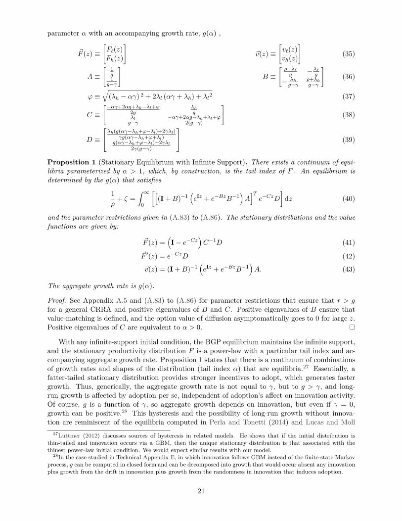
parameter α with an accompanying growth rate, g(α) ,

~F (z) ≡[F`(z)Fh(z)

]~v(z) ≡

[v`(z)vh(z)

](35)

A ≡[ 1

g1

g−γ

]B ≡

[ρ+λ`g −λ`

g

− λhg−γ

ρ+λhg−γ

](36)

ϕ ≡√

(λh − αγ) 2 + 2λl (αγ + λh) + λl2 (37)

C ≡[−αγ+2αg+λh−λl+ϕ

2gλhg

λlg−γ

−αγ+2αg−λh+λl+ϕ2(g−γ)

](38)

D ≡λh(g(αγ−λh+ϕ−λl)+2γλl)

γg(αγ−λh+ϕ+λl)g(αγ−λh+ϕ−λl)+2γλl

2γ(g−γ)

(39)

Proposition 1 (Stationary Equilibrium with Infinite Support). There exists a continuum of equi-libria parameterized by α > 1, which, by construction, is the tail index of F . An equilibrium isdetermined by the g(α) that satisfies

1ρ

+ ζ =∫ ∞

0

[[(I +B)−1

(eIz + e−BzB−1

)A]Te−CzD

]dz (40)

and the parameter restrictions given in (A.83) to (A.86). The stationary distributions and the valuefunctions are given by:

~F (z) =(I− e−Cz

)C−1D (41)

~F ′(z) = e−CzD (42)

~v(z) = (I +B)−1(eIz + e−BzB−1

)A. (43)

The aggregate growth rate is g(α).

Proof. See Appendix A.5 and (A.83) to (A.86) for parameter restrictions that ensure that r > gfor a general CRRA and positive eigenvalues of B and C. Positive eigenvalues of B ensure thatvalue-matching is defined, and the option value of diffusion asymptomatically goes to 0 for large z.Positive eigenvalues of C are equivalent to α > 0.

With any infinite-support initial condition, the BGP equilibrium maintains the infinite support,and the stationary productivity distribution F is a power-law with a particular tail index and ac-companying aggregate growth rate. Proposition 1 states that there is a continuum of combinationsof growth rates and shapes of the distribution (tail index α) that are equilibria.27 Essentially, afatter-tailed stationary distribution provides stronger incentives to adopt, which generates fastergrowth. Thus, generically, the aggregate growth rate is not equal to γ, but to g > γ, and long-run growth is affected by adoption per se, independent of adoption’s affect on innovation activity.Of course, g is a function of γ, so aggregate growth depends on innovation, but even if γ = 0,growth can be positive.28 This hysteresis and the possibility of long-run growth without innova-tion are reminiscent of the equilibria computed in Perla and Tonetti (2014) and Lucas and Moll

27Luttmer (2012) discusses sources of hysteresis in related models. He shows that if the initial distribution isthin-tailed and innovation occurs via a GBM, then the unique stationary distribution is that associated with thethinest power-law initial condition. We would expect similar results with our model.

28In the case studied in Technical Appendix E, in which innovation follows GBM instead of the finite-state Markovprocess, g can be computed in closed form and can be decomposed into growth that would occur absent any innovationplus growth from the drift in innovation plus growth from the randomness in innovation that induces adoption.

21

(2014). Furthermore, adoption and aggregate growth are a function of the shape of the distribution,but the shape of the distribution is determined by the initial distribution or exogenous stochasticparameters, not endogenously by the interaction of adoption and innovation activity. In the nextsection, we compute the finite-support BGP—which comes about from finite initial conditions—andcompare its properties with those of the infinite-support case.

3.2 Stationary BGP: Finite Unbounded Relative Support

In this section, we study the BGP equilibrium in the case when the initial distribution Φ (0, Z) hasfinite support. Due to the bounded growth rates of the Markov process, if the support of Φ(0, z) isfinite, then it remains finite as it converges to a stationary distribution. Recall that, with a finitefrontier, g ≤ γ to have a BGP with non-degenerate Fi(z). Hence, in the stationary equilibrium,there are no h-type agents hitting the adoption threshold (and the smooth-pasting condition for hfirms is not a necessary condition). As will become clear when we contrast bounded and unboundedsupport examples in Section 3.3, the g = γ case is the most natural, and the g < γ cases occur onlyas knife-edge results.

In this section and the rest of the paper, for simplicity we consider the process of adopting newtechnologies disruptive to R&D, in that an adopting firm becomes an ` type regardless of its formertype.29 That is,

F`(z) = F`(z) + Fh(z) = F (z) (44)Fh(z) = 0. (45)

Necessary conditions for a stationary equilibrium with a finite initial frontier are v`(z), vh(z),F`(z), Fh(z), and S—such that (23) to (25), (27) and (30), and

ρvh(z) = ez + λh(v`(z)− vh(z)) (46)

v(0) = 1ρ

=∫ z

0v`(z)dF (z)− ζ (47)

0 = gF ′`(z) + SF (z) + λhFh(z)− λ`F`(z)− S (48)0 = λ`F`(z)− λhFh(z) (49)

Define the constants, λ ≡ λ`λh

and λ ≡ λ`ρ+λh + 1.

Proposition 2 (Stationary Equilibrium with Finite Unbounded Support). There exists a uniquemaximum growth equilibrium with g = γ and z → ∞. There does not exist an equilibrium withfinite and bounded support.

The unique stationary distribution is,

F`(z) = 11+λ

(1− e−αz) (50)

Fh(z) = λF`(z), (51)

where α is the tail index of the power-law distribution:

α ≡ (1 + λ)F ′`(0), (52)29Unlike the infinite-support case in Section 3.2, important properties of the finite-support equilibria are not

sensitive to the degree of correlation in the draws, and we have simply chosen the most analytically convenient.

22

and F ′`(0) is determined by model parameters:

F ′`(0) =

λh

(ζ(ρ+γ)((ρ+γ)+λh+λ`)−

√ζ

((4γ+(ρ+γ)2ζ

)(−γ+(ρ+γ)+λh)2+2(−2γ+(γ−(ρ+γ))(ρ+γ)ζ)(γ−(ρ+γ)−λh)λ`+(γ−(ρ+γ))2ζλ`2

)+ζγ22+ζ(−γ)(3(ρ+γ)+2λh+λ`)

)γ2ζ(λh+λ`)(γ−(ρ+γ)−λh) .

(53)

The firm value functions are,

v`(z) = λ

γ + ρλez + 1

ρ(ν + 1)e−νz (54)

vh(z) = ez + λhv`(z)ρ+ λh

, (55)

where ν is defined as

ν ≡ ρλ

γ> 0. (56)

Proof. See Appendix A.3.

Proposition 2 shows that while, initially, finite-support distributions maintain finite support forall t < ∞, stationary distributions all have asymptotically infinite relative support. That is, theratio of frontier to lowest productivity goes to infinity: z → ∞. Given the Markov process for `and h, there will be some agents who hit lucky streaks more than others, escape from the pack, andbreak away. There is no finite bounded BGP because a diminishing, yet strictly positive numberof firms at the frontier keep getting lucky and grow at γ forever.30

Why don’t the low-productivity firms simply adopt more rapidly to maintain a compact dis-tribution? The reason is that although the mass of firms near the frontier is always positive, thenumber of such firms is vanishingly small. Consequently, the probability an adopting firm willadopt technologies near the frontier becomes arbitrarily close to zero.

The value functions given by equations (54) and (55) have an intuitive interpretation that isinformative about firms’ adoption incentives and behavior. The stationary value of an h firm is thatit will continue to produce with its current z continually earning flow profits ez, discounted for timeand accounting for the probability that it will switch to being an ` type at rate λh. Similarly, an `firm values producing with its current z earning flow profits ez, discounting for time and switches toh, but also considers that its productivity is falling behind relative to innovators who are growingat rate γ. Furthermore, since it is the ` firms that adopt in equilibrium, they have an extra termthat captures the option value of being able to adopt. The elasticity parameter ν measures howthe adoption option value decreases with higher productivity. A firm with higher productivity willtake longer in expectation to fall back to the adoption threshold, and, thus, higher-productivityfirms place less value on the option to adopt. Note that ν > 0 shows that in the unbounded casewith z →∞, in the limit, firms at the frontier place no value on the option to adopt.31

By comparing Propositions 1 and 2, we see that the assumption that the distribution has infinite-support at time zero is not innocuous. When the initial distribution has infinite-support, there isa continuum of BGP equilibria indexed by the tail parameter of the stationary distribution (α),with each initial distribution mapping to a particular α. In this infinite-support case, aggregategrowth can be faster than the rate of innovation—i.e., g(α) > γ or latent growth. In contrast,

30This result is robust to variations in the diffusion specification, including assuming that adopting agents drawfrom the Fh(z) distribution and start with an h type, which adds the strongest incentives to increase diffusion andcompress the distribution.

31This interpretation applies more generally to other models with knowledge diffusion. For example, a similarresult would hold in Lucas and Moll (2014) or Luttmer (2015b), where the “option value” in our model would be thecomponent of the value function that captures the opportunities to learn from agents with higher productivity.

23

the BGP in the finite unbounded case—which asymptotically features a power-law distributionwith an unbounded relative support (z →∞)—has a unique maximum-growth induced stationarydistribution that is independent of the initial distribution and has g = γ.

Thus, in the finite unbounded economy with exogenous innovation, adoption affects the shapeof the distribution, but the aggregate growth rate is determined solely by the innovation rateparameter γ. When γ is a choice and growth is endogenous, the option value of adoption forfrontier firms will influence whether and how adoption affects long-run growth.

3.2.1 Equilibrium with g < γ

While we have concentrated on equilibria with maximum growth, g = γ, there may be otherequilibria with g < γ. This is the equivalent to latent growth, but with a negative sign. Intuitively,the initial conditions of the economy are dragging it down so that a particular BGP growth rate iskept below the innovation rate. An initial condition with a different arrangement of productivitiesthat provided better adoption incentives could bring the aggregate growth rate up to the innovationrate.

Proposition 3 (Finite Unbounded Equilibrium with g < γ). For both a infinite- and finite-support initial conditions, there exists a continuum of equilibrium parameterized by α > 1, which,by construction, is the tail index of the productivity distribution. An equilibrium is determined bythe aggregate growth rate g(α) < γ that satisfies

1ρ

+ ζ = a2b1

(a3

α+ β2− a3b2α+ β2

− 1α+ β1

+ b2α+ β1

)+ a1b1

( 11− α + b2

α− 1

)(57)

given a1, a2, a3, b1, b2, β1, β2, and α defined in (A.103), (A.108) to (A.110) and (A.112) to (A.114).

Proof. See Appendix A.6. Parameter restrictions are given in (A.116), (A.120) and (A.121).

The example of Figure 18 shows continuity from the endogenous α at the g = γ solutioncalculated in Section 3.2 to lower g as the tail thins out. However, as we will see in Section 3.3, theg < γ cases disappear whenever there are conditions that generate a finite bounded distribution.

The low-productivity firms don’t adopt fast enough to keep up with the innovation rate forreasons similar to why there is no bounded equilibrium. As the mass of the lucky agents withextremely high z thins out, it doesn’t strongly affect the diffusion incentives and adoption proba-bilities of those with a low z. The reason that adopters don’t find it worthwhile to keep up is thatthe mean can expand more slowly than the frontier. The incentive for adoption, which drives thespeed of the moving barrier at the minimum of the distribution, is given by the expected draw inproductivity. Therefore, if the frontier diverges to infinity, but the mean doesn’t keep growing atthe same rate, the frontier technology will diverge.32

Possible multiplicity in the g < γ direction is less concerning than the g > γ case, because itis easy to believe there is a possibility that innovations are inefficiently disseminated across theeconomy. Essentially, since not all firms are growing at the rate γ, if the tails are thin enough, thenthe incentives for adopting—conditional on that particular distribution shape—can be insufficientto maintain aggregate growth at the rate of the frontier. However, as Section 3.3 demonstrates, thismultiplicity is unstable and is eliminated as soon as there is any chance of jumping to the frontier.

32Given a fixed barrier, the logic is similar to the linear or asymptotically linear Kesten processes bounded awayfrom zero with affine terms, for which, under appropriate conditions, the asymptotic tail index can be explicitlycomputed in terms of the stationary distribution induced by the Markov process. In our model, however, theadoption process introduces non-linear jumps that are not multiplicative in productivities and that do not permitthe simple characterization of the tail index. The endogenous absorbing adoption barrier (which acts like a reflectingbarrier with stochastic jumps) complicates the analogy since it moves according to the optimal adoption behavior offirms.

24

Loosely speaking, in models with Schumpeterian forces, g < γ equilibria would not exist and latentgrowth would never have a negative sign.

3.2.2 Extension to Distorted Adoption Distribution

The reason that there is no bounded support BGP is that the adopters don’t keep up with theinnovators at the frontier. We can modify the adoption process so that the Z is drawn from a dis-tortion of the unconditional distribution, twisting the distribution so that adopters are either moreor less likely to get better technologies compared to drawing from the unconditional distributionF .33 We show that unboundedness is a rather robust result, in the sense that higher chances ofadopting better technologies are not enough to generate bounded equilibria.

The distortion, representing the degree of imperfect mobility or beneficial adoption prospects,is indexed by κ > 0, where the agent draws its Z from the CDF Φ(t, Z)κ. Note that for higher κ,the probability of a better draw increases.The stationary normalized adoption distribution is

F`(z) = (F`(z) + Fh(z))κ = F (z)κ (58)Fh(z) = 0. (59)

We write F (z)κ for the normalized draw process.Necessary conditions for a stationary equilibrium with a finite initial frontier are v`(z), vh(z), F`(z),Fh(z), and S—such that (23) to (25), (27), (30) and (46), and

v(0) = 1ρ

=∫ z

0v`(z)dF (z)κ − ζ (60)

0 = gF ′`(z) + SF (z)κ + λhFh(z)− λ`F`(z)− S (61)0 = λ`F`(z)− λhFh(z). (62)

Corollary 2. There does not exist an equilibrium with finite and bounded support for any κ > 0.Furthermore, κ distorts the unique tail parameter of the (asymptotically) power-law stationarydistribution.

Proof. See Technical Appendix C.4.

Modifying κ may provide a better description of the adoption process and allow for an improvedfit to the data for the shape of the stationary productivity distribution. Nonetheless, smoothlytwisting the adoption distribution so that firms obtain substantially better technologies with highprobability is not enough to compress the distribution by allowing adopters to keep up with thefrontier. In the next section, we extend the model to obtain existence of BGP with a finite boundedstationary distribution. The bounded and unbounded equilibria are similar in many ways, butcomparison of the firm value functions will show how adoption affects innovation once firms choosehow fast to innovate.

3.3 Stationary BGP: Finite Bounded Relative Support

For a finite bounded equilibrium to exist, Proposition 2 shows that it is not enough that adoptershave a set of adoption possibilities growing with the scale of the economy. Rather, there mustbe some way that firms not at the frontier can catch up to those few lucky firms that have beenh-hypes at the frontier forever. In this section, we extend the model by introducing another typeof productivity-enhancing activity to construct finite bounded BGP equilibria.

33While κ is exogenous here, in Section 5, we solve a version of the model in which κ is endogenous. We interpretthe choice of κ as limited directed search, in that, at some cost, firms can focus their attention on adopting bettertechnologies with higher probability.

25

This section helps us to further understand the hysteresis and deviations from g = γ. Recallthat the multiplicity with g > γ inherent in the infinite-support case of Section 3.1 was eliminatedbecause we both bounded the growth rates and assumed a finite initial condition on the distribution.However, this left a possibility of g < γ. In this section, we will show that conditions generating afinite bounded relative support also ensure a unique equilibrium with g = γ.

One motivation for modeling a bounded relative support is that, regardless of the commodityspace or model of competition, for all practical purposes, a firm grossly less productive than thefrontier—whether 100×, 1000×, or larger, but at some point—likely could not survive in a mar-ket populated by firms with such better technology. The more productive firms would move in,undercut, displace, and capture the market, or be imitated. In some sense, this bounded frontiermodel provides an intermediate case between Schumpeterian models, in which one or two firms atthe frontier dominate all production, and the infinite dispersion model, in which firms of radicallydifferent productivities coexist. A bounded frontier also seems consistent with the, admittedly, lim-ited evidence on the stability of the right tail of the relative firm size distribution, which Luttmer(2010) shows have been constant since 1977 using the Business Dynamics Statistics data.

In this section, we show that the bounded frontier case that seems reasonable on first principleshas important implications for the determination of the aggregate growth rate and for how adoptionand innovation interact. In the exogenous growth context, this bounded frontier case is a buildingblock for the model with a frontier that evolves endogenously in response to innovation decisionsof high-productivity firms developed in Section 4.2. As will become clear, an important interactiondetermining the endogenous growth rate appears in the decisions of firms at the frontier. With anunbounded frontier, frontier firms are arbitrarily far away from the adoption threshold, and, thus,the interactions between technology adoption and innovation are limited, unlike in this boundedcase.

An alternative way to model within-firm productivity change is to assume that firms havesome chance of leapfrogging to the frontier. Such leapfrogging is a continuous-time version of aquality-ladders model.34 For generality, the jumps can occur either for adopting or for innovatingfirms. Innovators jumping to the frontier represents some chance that the innovation processgenerates a big insight, instead of steady incremental progress. Different from autarkic innovationthat generates γ proportional growth through process improvement, leapfrogging may be viewedas a melding of innovation and diffusion since the jump is a function of the existing productivitydistribution. Adopters jumping to the frontier captures that sometimes adopters get lucky, andtheir search for a new technology finds the best one available. For tractability, we model such ajump as temporarily disruptive to innovation, such that all leapfrogging firms become `−types andmust wait for the Markov transition to h before they become innovators again.35

We modify the model that generated finite unbounded BGP, as characterized in Proposition 2,by adding an arrival rate of jumps to the frontier, η ≥ 0, as depicted in Figure 4.

In principle, there could be a jump discontinuity in the CDF F (z) at z. Due to right continuity34In a continuous-time model with leapfrogging event arrivals that generate a multiplicative step above the frontier,

the frontier would become infinite immediately, as there would be some agent with an arbitrarily large number ofjump arrivals in any positive time interval (as in König, Lorenz, and Zilibotti (2016)). An alternative process withsimilar qualitative implications is to recast leapfrogging as a step-by-step innovation model in the spirit of Aghion,Akcigit, and Howitt (2014). In either case, infinite support allows for the possibility of latent growth.

35The assumption that all leapfroggers switch to the ` state is purely for analytical convenience and can bechanged without introducing qualitative differences. If some firms leapfrogged to the h state instead, then a rightdiscontinuity in Fh(z) would exist (∆h > 0) and more care would be necessary in solving the KFE and integrating thevalue-matching condition. Furthermore, this simplification ensures that the values of jumps to the frontier remainidentical for both agents, and, hence, both types have the same adoption threshold, as demonstrated in Appendix A.2.With this specification, a possible downside is that v`(z) < vh(z − ε) for some set of small ε, and those firms wouldrather keep the lower z rather than innovate. In the calibrated model, the difference between v` and vh is tiny dueto high switching probabilities, and, thus, this is binding for a very small number of firms.

26

0 z z

vi(z)

vi(0)

λh

λℓ

vh(z)

vℓ(z)

η

η

Figure 4: Normalized, Stationary Value Functions with Bounded Support

of the CDF, the mass at the discontinuity z = z is

∆i = limε→0

(Fi(z)− Fi(z − ε)) . (63)

When all leapfrogging firms become type `, we can show that Fi(z) are continuous and ∆` = ∆h = 0.This is because type ` firms immediately fall back in relative terms and don’t pool at the frontier.As those firms falling back also jump back and forth to the h type, the F`(z) and Fh(z) distributionsmoothly mix, ensuring continuity.

Define H (z) as the Heaviside operator. Along with (23) to (25) and (30), the following charac-terizes the necessary conditions for a stationary equilibrium:

ρv`(z) = ez − gv′`(z) + λ`(vh(z)− v`(z))) + η(v`(z)− v`(z)) (64)ρvh(z) = ez + λh(v`(z)− vh(z)) + η(v`(z)− vh(z)) (65)

0 = gF ′`(z) + λhFh(z)− λ`F`(z)− ηF`(z) + ηH (z − z) + SF (z)− S (66)0 = λ`F`(z)− λhFh(z)− ηFh(z). (67)

While the value-matching condition is identical to equation (47) in the unbounded setting, thevalue of adopting is now dependent on the value at the frontier:

v(0) = 1 + ηv`(z)ρ+ η

=∫ z

0v`(z)dF (z)− ζ. (68)

Define the constants, λ ≡ λ`η+λh , λ ≡

ρ+λ`+λhρ+λh , and ν = ρ+η

γ λ.Proposition 4 (Stationary Equilibrium with a Bounded Frontier). Given parameter restrictions,a unique equilibrium with z <∞ exists with g = γ. The stationary distribution is

F`(z) = F ′`(0)(F ′`(0)− η/γ)(1 + λ)

(1− e−αz) (69)

Fh(z) = λF`(z), (70)

with

α ≡ (1 + λ)(F ′`(0)− η/γ) (71)

z = log(γF ′`(0)/η)α

. (72)

27

The equilibrium F ′`(0) solves the following implicit equation (substituting for α and z),

ζ + 1ρ

=γF ′`(0)αλ

(− e−νz(−1+e−αz)η

ραν + ezη(e−αz−1)−αρ + −e−(α+ν)z+1

ν(α+ν) + −ez−αz+1α−1

)γ(γF ′`(0)− η)(ν + 1) . (73)

The value functions for the firm are,

v`(z) = λ

γ(1 + ν)

(ez + 1

νe−νz + η

ρ

(ez + 1

νe−νz

))(74)

vh(z) = ez + (λh − η)v`(z) + ηv`(z)ρ+ λh

. (75)

Proof. See Appendix A.4. Parameter restrictions include those such that the F ′`(0) that solvesequation (73) is larger than η/γ. A proof of uniqueness, showing that g < γ equilibria do not exist,is in Appendix A.7.

As before, α represents the shape of the productivity distribution. The α is an empirical “tailindex” that can be estimated from a discrete set of data points. Unlike in the unbounded case,z is now bounded, and, hence, this tail index is better interpreted as the shape parameter of aright-truncated power-law.

In contrast to the finite unbounded BGP, the Bellman equations (74) and (75) now contain thevalue of production and the option value of adoption for the frontier z. That is, in addition to thevalue of production with current z modified by time discount and the probabilities of switchingi-type, the value function accounts for the chance of jumping to the frontier. Thus, movementsin the frontier provide enough incentive for adopters at the bottom of the distribution to keep upwith the frontier, allowing for a bounded stationary distribution.

As noted at the end of the previous section, leapfrogging to the frontier by a positive massof agents can contain the escape in relative productivities by lucky firms that get streaks of longsojourns in the high-growth group h. As they eventually lose their innovative ability and become`-types, they will be overtaken by others that leapfrog to the frontier from within the productiv-ity distribution and replenish it. This leapfrogging/quality ladder process prevents almost everylaggard from remaining a laggard forever. The distribution of relative productivities then remainsbounded, as the frontier acts as a locomotive in a relay race. Note that this locomotive processis similar to models of technology diffusion in which the growth rate of adopters is an increasingfunction of the distance to the frontier, unlike this model of innovators with multiplicative growthin their productivity level (see, e.g., Nelson and Phelps (1966) and Benhabib, Perla, and Tonetti(2014)). If adopters were to fall behind, they would adjust their behavior, endogenously increas-ing their adoption activity to match innovators’ growth rates, ensuring that relative productivitieswould be bounded in equilibrium.

Additionally, now that the relative frontier is bounded, in the long run, frontier firms stillplace positive value on the option to adopt. This means that increases in the value of adoption,either associated with lower costs or higher benefits of adoption, will affect the value of frontierfirms. Depending on how far the frontier is from the adoption threshold, in the endogenous growthenvironment changes in the value of adoption will influence innovation behavior, which may affectaggregate growth rates.

Before moving to the endogenous growth case in the next section, we compute a finite boundedequilibrium with calibrated parameter values and use comparative statics to illustrate propertiesof the economy. The calibration is designed to set roughly set parameters in the relevant regionof the state space. Details of the calibration are discussed in Appendix D.6. We set γ = .02 totarget a 2 percent growth rate and ρ = 0.01 to generate a real interest rate of 3 percent. Transition

28

rates λh and λ` are chosen to roughly match firms’ growth-rates, with firms growing faster than5 percent annually labeled h types and all other firms labeled `-types. While the transition ratesare sensitive to the h-threshold growth rate, all resulting numerical analysis is unchanged by widevariation in this threshold, as all calibrated transition rates are high enough to suggest that thereis little persistence in either state and that the process essentially acts like iid growth rates. Wetarget a tail index α = 2.12, which corresponds to a tail parameter of 1.06 in the size or profitsdistribution in a monopolisitic competition model, as used in Luttmer (2007). We target z = 1.61(i.e., the frontier to minimum productivity ratio is 5). This ratio is larger than the z = 0.651(1.92 ratio in levels) documented by Syverson (2011) between the top and bottom decile withinnarrowly defined industries, and is closer to the 5:1 ratio found in Hsieh and Klenow (2009) in Indiaand China. Alternatively, comparing the largest to smallest firms in the economy yields a muchlarger 279:1 ratio ( z = 5.63), which is numerically close to ∞ for all intents and purposes in thismodel. The resulting parameterization is γ = 0.02, ρ = 0.01, λ` = 0.533, λh = 1.128, and ζ = 25.18η = 0.00098.

First, as shown in Figure 5, v` and vh are very similar because the calibrated λi are large, and,thus, the extra benefit of being in the high state or the relative pain from being in the low statedoes not last very long. Second, the distributions Fi are truncated power-law shaped, with manylow-productivity firms and few high-productivity firms, but is truncated above at the z relativefrontier. In this calibration, there are also fewer h firms than ` firms at all productivities.

Comparative statics on how changes in η, γ, ζ, and λh affect z and α are shown in Figure 6.Easier innovation, in the sense of a higher growth rate for innovators, spreads out the distribution,creating a more distant technology frontier and a thicker tail. Easier leapfrogging, in the sense ofa higher probability of jumps to the frontier, also generates thicker tails but generates less of aproductivity gap between the best and worst firms. Easier adoption, captured by lower costs ζ,compresses the distribution, shrinking the relative frontier and thinning the tail.

0 0.5 1 1.5

100

150

200

250

0 0.5 1 1.5

0

0.5

1

1.5

zz

vℓ(z)vh(z)

F ′ℓ(z)

F ′h(z)

Figure 5: Exogenous vi(z), and F ′i (z) with a Bounded Frontier

3.4 Stationary BGPs with Exogenous Innovation: Summary and Analysis

An analysis of BGP equilbria with exogenous growth points to economically important differencesbetween economies with infinite-support, finite bounded support, and finite bounded support dis-tributions. There are two major difference between infinite- and finite-support BGPs. First, withfinite-support, the aggregate growth rate must be weakly less than the growth rate of innovators,

29

0.005 0.01 0.015 0.02

1

1.5

2

2.5

0

0.5

1

1.5

2

2.5

3

0.01 0.015 0.02 0.025 0.03

1.4

1.6

1.8

1.5

2

2.5

15 20 25

1.4

1.5

1.6

2

2.5

3

0.5 1 1.5 2

1.5

1.6

1.7

2

2.2

2.4

η

zz

z

z

αα

α

α

γ

ζ λh

Figure 6: Comparative Statics with a Bounded Frontier

while in the infinite-support case the aggregate growth rate can exceed the growth rate of innova-tors. Second, in the finite unbounded case, there is still the possibility of growth rates strictly lessthan the innovation rate. Finally, in the finite bounded support case, there is no such hysteresis;there is a unique equilibrium stationary distribution and a growth rate g = γ. Since the finitebounded cases’ unique BGP occurs for an arbitrarily small arrival rate of jumps (i.e., η → 0), wefocus attention on the equilibrium with g = γ even in the finite unbounded case.

These results on infinite-support distributions arise when the initial distribution has infinite-support but can be mapped to models that generate infinite-support distributions from arbitraryfinite-support initial conditions—such as the GBM models discussed previously. In those cases, theresult is stronger: any sort of stochastic shocks with unbounded growth rates generate a contin-uum of stationary distributions and growth rates, which can have a growth rate greater than theinnovation rate.

We live in a finite-support world: there is no firm operating at any point in time with the besttechnology that could ever be invented and there were no car manufacturers in the Stone Age.While it may be appropriate for certain questions, because the economic properties of infinite- vs.finite-support equilibria are so different, using an infinite-support assumption as an approximationto finite-support requires caution.

Even for finite-support distributions, when normalized, the relative frontier of best to worstfirms could be bounded or could be diverging to infinity. We showed that in order to maintaina bounded relative frontier, there needs to be some way for laggards to keep up with the frontierinnovators by, for example, leapfrogging. Beyond eliminating the g < γ hysteresis, the key differencebetween the bounded and unbounded cases appears in the option value of adoption for firms at thefrontier. In the bounded equilibrium, even the best firm realizes that it may become an adopterin some reasonable time frame and places some positive value on the option to adopt. Since it isthe innovative firms with the highest productivity that push out the frontier, this creates a linkbetween their innovation incentives and the value of adoption, through which a change in the costof the benefits of adoption will affect aggregate growth. In Section 4, we study this interactionbetween adoption and innovation in an endogenous growth version of the model.

30

4 Stationary Equilibria with Endogenous Stochastic InnovationThis section introduces endogenous innovation into the stochastic model with finite-support. Weassume that firms can control the drift of their innovation process, as in Atkeson and Burstein(2010) and Stokey (2014). In Section 4.1, in order to analyze the unbounded case with z →∞ wefirst assume that the arrival rate of jumps to the frontier, η, is zero. This allows us to focus onthe link between innovation and aggregate growth before adding the complication of the aggregategrowth rate being affected by the option value of adoption for innovators at the frontier. Then, inSection 4.2, we move to the model with jumps to the frontier and bounded support and analyzehow the innovation choice of frontier firms is influenced by the option value of adoption, whichaffects the aggregate growth rate. Thus far, the main link between innovation and adoption isthrough the option value of adoption. In Section 5, we also model technology as excludable, andallow adopting firms to bargain with the owner of the technology that they are trying to adopt.We show how payments from adopters affect innovation investments and aggregate growth.

For simplicity, we model the innovation choice with no direct spillovers from other firms, in orderto focus on the new interactions that we are modeling. With this simplification, the interactionshere arise via tradeoffs in the firms’ choices, rather than via a coupled innovation and adoptiontechnology.36

To model endogenous innovation, a firm in the innovative state can choose its own growth rateγ ≥ 0 subject to a convex cost proportional to its current Z. Let χ > 0 be the productivity of itsR&D technology and the cost be quadratic in the growth rate γ. Thus the h-firm Bellman becomes

ρvh(z) = maxγ≥0

ez − (g − γ)︸ ︷︷ ︸Drift

v′h(z)− 1χe

zγ2︸ ︷︷ ︸R&D cost

+λh(v`(z)− vh(z)) + η(v`(z)− vh(z))

(76)

The key additional necessary equilibrium condition in the endogenous growth model comes fromthe first-order condition associated with optimal innovation rates:

γ(z) = χ2 e−zv′h(z). (77)

Thus, the value function of the h-firm in (76) becomes the following non-linear ODE:

ρvh(z) = ez − gv′h(z) + χ4 e−zv′h(z)2 + λh(v`(z)− vh(z)). (78)

Instead of all h-firms growing at rate γ exogenously, h-firms are now choosing a growth rate γ thatis a function of their current productivity level, z.37

Adapting the equations in Section 3.3, the equations that characterize an equilibrium are (23)to (26), (30), (31) and (68) with the following Bellman and KFE equations:

ρv`(z) = ez − gv′`(z) + λ`(vh(z)− v`(z)) + η(v`(z)− v`(z)) (79)ρvh(z) = ez − gv′h(z) + χ

4 e−zv′h(z)2 + λh(v`(z)− vh(z)) (80)

0 = gF ′`(z) + +λhFh(z)− λ`F`(z)− ηF`(z) + ηH (z − z) + SF (z)− S` (81)0 = (g − γ(z))︸ ︷︷ ︸

Drift

F ′h(z) + λ`F`(z)− λhFh(z)− ηFh(z)− Sh. (82)

36This is in contrast to Schumpeterian models, where innovations are built upon on diffusion from the frontier,and approaches such as that of Chor and Lai (2013), who are interested in the direct interaction with a dependentinnovation process, with aggregate spillovers of knowledge.

37As the choice of γ is increasing in z in equilibrium, agents in the h state will end up crossing the endogenousadoption threshold, as shown in Appendix A.2, and, thus, the smooth-pasting condition for h types is now neces-sary. To generalize the approach, different innovation types are best understood as having different productivity ininnovation, χ, with the bellman equation for each type as (78).

31

Numerical Methods. For all endogenous growth cases, the need to jointly solve for the nonlinearHamilton-Jacobi-Bellman equations and the Kolmogorov forward equations necessitates non-trivialnumerical solution methods. The problem takes the form of a set of ODEs with parameters con-strained by equilibrium conditions that are themselves functions of the solutions to the ODEs.We compute the equilibrium using a generally applicable numerical technique based on spectralcollocation and quadrature, as detailed in Technical Appendix B.38

4.1 Endogenous Innovation with a Finite Unbounded Frontier

In this section, we study the finite unbounded BGP, which is the case corresponding to η = 0.

Proposition 5 (Endogenous Innovation and Finite Unbounded Support BGP). For η → 0, aunique equilibrium exists with a growth rate that is the solution to the cubic equation39

g(g2 + g(2λh + λ` + 3ρ) + 2ρ(λh + λ` + ρ)

)= χ(g + λh + λ` + ρ). (83)

The endogenous innovation choice is such that γ(0) = 0 and limz→∞ γ(z) = g.

Proof. See Appendix B. The numerical method to compute the equilibrium γ(z) and Fi(z) isdescribed in Technical Appendix B.

In addition to the existence and uniqueness of the equilibrium, a main result is that the inno-vation rate is increasing in productivity—i.e., γ′(z) > 0. There is a tradeoff in firms’ innovationdecisions: investing more in innovation grows their productivity and increases their profits, butfirms with higher productivity are further from the adoption threshold and, thus, have a smalleroption value of adoption. Since the option value of adoption is a larger component of total value forlower-productivity firms, the low productivity firms invest less in innovation. Intuitively, for a firmjust above the adoption threshold, why invest in innovation to get an incremental improvementwhen they can save the cost of innovating and, instead, adopt a technology discretely better inexpectation than the one it is currently operating? Of course, the cost of adopting and innovatingwill jointly determine this adoption threshold.40

The innovation rate and statistics of the productivity distribution for a computed equilibriumare presented in Figure 7. In addition to the calibration discussed in Section 3.3, the innovation costparameter χ = 0.001074 is calibrated to match g = 0.02 and ζ = 27.2 to match the tail parameterof α = 2.12.

In order to get a sense of the shape of the unconditional distribution, we define the “local” tailindex

α(z) ≡ F ′(z)1− F (z) . (84)

In the standard log-log plot used for estimating power-laws, as in Gabaix (2009), this α(z)would be the slope of the non-linear equation at z. Note that with this definition, the “local” tail

38The technique uses a simple trick: line up the collocation nodes for the function approximation with those ofthe quadrature nodes for calculating expectations and equilibrium conditions. After everything is lined up, you cannaively stack every equation in the model, including the Bellman Equations, KFEs, equilibrium conditions, etc. intoa single nonlinear system of equations, and solve without any nested fixed points. In practice, this requires using ahigh-performance solver and auto-differentiation, but is easy to implement and reasonably fast.

39The limit is necessary here for uniqueness, because otherwise a g < γ growth rate along the lines of Section 3.2.1is possible and (83) only determines γ(∞). For the same reasons as discussed in Section 3.2.1 we do not focus on thenegative latent growth cases here.

40Research that separates internal innovation on existing products from Schumpeterian innovation replacing prod-ucts, such as Akcigit and Kerr (2016), find that internal innovation scales moderately faster with size. Since allinnovation in our model is “internal innovation” of this sort, this is consistent with our result that innovation ratesare increasing in productivity.

32

0 1 2 3 4

0

0.005

0.01

0.015

0.02

0 1 2 3 4

0

0.2

0.4

0.6

0.8

0 1 2 3 4

1.5

1.6

1.7

1.8

1.9

2

2.1γ(z)

zzz

Fℓ(z)Fh(z) α(z)

Figure 7: Endogenous γ(z), Fi(z), and α(z) with a Finite Unbounded Frontier

index of a Pareto distribution is constant and equal to its true tail index. Furthermore, for anydistribution with infinite-support, the tail index is α ≡ lim

z→∞α(z). Figure 7 plots the local tailcoefficient, converging to the calibrated value of 2.12. As the tail index is increasing, this showsthat there is more productivity dispersion for firms with lower relative productivity.

22 24 26 28 30 32

0.02

0.022

0.024

0.026

0.028

22 24 26 28 30 32

1.6

1.7

1.8

1.9

2

2.1

2.2

2.3

22 24 26 28 30 32

0.47

0.472

0.474

0.476

ζζζ

g α Gini

Figure 8: Comparative Statics on Adoption Cost

The endogenous aggregate growth rate is the growth rate chosen by innovators at the frontier.As alluded to in the exogenous growth sections, now that aggregate growth is endogenous, we cansee that, in the unbounded case, the aggregate growth rate is independent of the cost of adoption.This is because innovating firms at the frontier have zero option value from adoption; therefore,changes in the cost or benefits of adoption do not alter their innovation behavior. Figure 8 plotscomparative statics for a change in the adoption cost. As the theory shows, the aggregate growthrate is invariant. However, changes in the cost of adoption affect the shape of the distribution.Higher adoption costs induce a significantly thicker tail, but almost no change in the Gini coefficient.

4.2 Endogenous Innovation with a Finite Bounded Frontier

In this section, we study the finite bounded BGP, which is the case corresponding to η > 0. For thesame reasons as discussed in the exogenous innovation case, without leapfrogging, lim

η→0z(η) =∞.

Proposition 6 (Stationary Equilibrium with Continuous Endogenous Innovation and BoundedSupport). The endogenous innovation choice is such that γ(0) = 0 and γ(z) ≡ g. A continuum ofequilibria exist, parameterized by a z.

33

Proof. See Appendix B. A numerical method to solve for the continuum of equilibria is describedin Technical Appendix B.

In the limit approaching the unbounded case, as η → 0, the upper bound on g equals theunbounded growth rate in Proposition 5. However, in the endogenous growth bounded distributioncase, there are a continuum of equilibria indexed by the frontier z, each with an associated aggregategrowth rate g(z).

Compared to Stokey (2014), who features a similar innovation process but differs in the treat-ment of adoption, here, the endogenous choice of γ is complicated by the option value of adoption.In the unbounded case, the aggregate growth rate—i.e., γ(z) as z → ∞—is unique because theoption value disappears, as opposed to when z is bounded. Different distributions and associatedz induce different growth option values, and allow for a continuum of self-fulfilling γ(z). That is, asmaller z increases the option value of adoption for innovators at the frontier, which is a disincentiveto innovate; this leads to less innovation at the frontier, which, consistently, generates a smallerz. The multiplicity here is due to complementarity of firm decisions and is fundamentally differentthan the g > γ latent growth multiplicity driven by initial conditions as discussed previously (seeAppendix C.1).

Since the option value of adoption is positive for innovators at the frontier, the aggregate growthrate is affected by adoption costs and benefits.41

0 0.5 1 1.5

0

0.005

0.01

0.015

0.02

0 0.5 1 1.5

0

0.1

0.2

0.3

0.4

0.5

0.6γ(z)

zz

F ′ℓ(z)

F ′h(z)

Figure 9: Endogenous γ(z) and F ′i (z) with an Bounded Frontier

A calibrated example of the optimal innovation policy and productivity distributions for abounded endogenous growth BGP is shown in Figure 9. Figure 10 documents the intuition thatlower z are associated with lower aggregate growth rates, due to the self-fulfilling balancing ofinnovation incentives. The larger the option value of adoption—which is increasing in the distanceof the relative frontier—the lower are the incentives to push out the frontier by innovation.

Figure 11 plots the maximum growth rate of the set of admissible g as a function of η, usingequation (83) with the same parameters used in Figure 7 (Endogenous Unbounded BGP). Asη → 0, the number of jumps to the frontier approaches 0, and the bounded model studied inSection 4.2 asymptotically becomes the unbounded model studied in Section 4.1. The intuitionfor a decreasing max(g(η)) is that with more jumps to the frontier, the distribution becomes morecompressed. As the growth rate of the frontier is determined by the innovation decision at z, which

41Due to the multiplicity of equilibria, comparative statics of stationary distributions are not well-defined. Numer-ically, we find that—fixing all parameters—the range of feasible g in these stationary equilibria tends to be fairlysmall. For example, Figure 10 contains all regions of g where the numerical algorithm converged.

34

1.5 2 2.5 3 3.5 4

0.019

0.0195

0.02

0.0205

0.021

0.0215

0

0.1

0.2

0.3

0.4

0.5

z

g(z)Gini(z)

Figure 10: Equilibrium g as a function of z

takes into account the option value of diffusion, the more compressed the distribution, the lowerthe innovation rate, for the same reasons that g(z) is increasing in Figure 10.

0.01 0.02 0.03 0.04

0.005

0.01

0.015

0.02

0.025

0.25

0.3

0.35

0.4

0.45

η

max g(η)Gini(η)

Figure 11: Maximum Equilibrium g(η) and associated Gini coefficient

5 Extensions: Licensing and Directed AdoptionIn this section, we combine all of the elements from earlier sections, and add additional features toendogenize all of the innovation and technology diffusion choices. These additions show that themodel is extensible and further highlight how adoption and innovation interact. The extension tolicensing brings the concept of variable degrees of excludability to models of technology diffusion.The extension to directed adoption captures that firms may be able to better target their adoptionactivities on technologies than if they merely obtain unconditional draws of the existing technologiesin use. This also gives the model flexibility to produce firm dynamics for adopters that may bemore consistent with the panel data.

35

Complete Nested Model (with Extensions). Since a firm may receive profits from licensingits technology, its profits no longer necessarily equal its productivity. We define π(z) to be thetotal profits of the firm, with π(z) = ez in the baseline model with no excludability. π(z) in themodel with licensing will be derived in Section 5.1. To endogenize leapfrogging, we allow firmsthat are adopting to jump to the frontier with probability θ ∈ [0, 1). Just as firms can choosetheir innovation rate γ subject to a convex cost, firms can also choose the probability of a jumpto the frontier with a convex cost. The cost of choosing jump probability θ is 1

ϑθ2. Thus, when a

firm upgrades its technology through adoption, it has some chance of adopting a state-of-the-artinvention and jumping to the frontier, and it can invest on the intensive margin to try to obtainsuch a large upgrade. Finally, we allow firms to choose the degree of distortion in their draws (i.e.,directed adoption) by choosing κ > 0 at a cost of 1

ς κ2. In this section, we adapt Sections 3.3 and 4.1

to include the endogenous innovation choice of γ, partial-excludability, a choice of θ, and a choiceof κ. The system of equations that characterize the equilibrium are (23) to (28), profits as definedin equation (98), and

ρv`(z) = π(z)− gv′`(z) + λ`(vh(z)− v`(z)) + η(v`(z)− v`(z)) (85)

ρvh(z) = maxγ≥0

{π(z)− 1

χezγ2 − (g − γ)v′h(z) + λh(v`(z)− vh(z)) + η(v`(z)− vh(z))

}(86)

v(0) = 1 + ηv`(z)ρ+ η

= maxθ≥0, κ>0

{(1− θ)

∫ z

0v`(z)dF (z)κ + θv`(z)−

1ψ

(ζ + 1

ϑθ2 + 1

ς κ2)}

(87)

0 = gF ′`(z) + λhFh(z)− λ`F`(z)− ηF`(z)+ (η + θ(S` + Sh))H (z − z) + (1− θ)(S` + Sh)F (z)κ − S` (88)

0 = (g − γ(z))F ′h(z) + λ`F`(z)− λhFh(z)− ηFh(z)− Sh (89)

See Appendix B for a nested derivation of all extensions. Note that when a particular firm choosesθ or κ, it does not influence the θ or κ chosen by the other firms. Firms will take into account theeffects of the aggregate “directed adoption” choice on Fi(z), and as all adopting firms are a prioriidentical, each firm will choose the same θ, which will induce an Fi(z) that is consistent with firms’beliefs about Fi(z) in equilibrium.

In addition to all other equilibrium requirements, the chosen intensity of jumps to the frontierfor adopting agents comes from the first-order condition of (87),

θ = ψϑ

2

∫ z

0v′`(z)F (z)κdz, (90)

and the directed technology diffusion choice from the first-order condition of (87) solves the implicitequation

κ = −ςψ(1− θ)2

∫ z

0v′`(z) log(F (z))F (z)κdz. (91)

5.1 Licensing and Partial Excludability

Up to now, the firm providing the underlying technology to the adopter was not able to preventbeing imitated—i.e., there was no excludability of the technology (no intellectual property protec-tion). To bring excludability to this environment with adopters and innovators, we model licensing,in which an adopting firm must pay a fee to the technology holder in order to adopt it. The feeis modeled as a portion of the present discounted value of adopting the technology and, instead ofbeing paid as a sequence of residual payments, the fee is paid up front in one lump sum. Firmsbargain to determine the size of the licensing fee, with the fee reflecting the bargaining power ofadopters and license issuers. There is no cost to the actual transfer of technology.

36

Bargaining. The timing is that the adopting firm first pays the adoption cost and then, upon therealization of the match, negotiations over licensing commence. Negotiations take the form of Nashbargaining, with a bargaining power parameter of ψ ∈ (0, 1]. ψ = 1 represents no excludability,in which the technology is adopted for free, without profit to the higher-productivity firm. Theoutside option of the adopting firm (i.e., the licensee) is to reject the offer and continue on withits existing technology—i.e., v(0). The outside option of the licensor is simply to reject the offerand gain nothing. From standard Nash bargaining, with a total surplus value of v`(z), let v be theproportion of the surplus obtained by the licensee and v`(z)− v be the proportion obtained by thelicensor. The Nash bargaining problem is

arg maxv

{(v − v(0))ψ(v`(z)− v)1−ψ

}. (92)

Solving for the surplus split, the value for a licensee that matches a firm with productivity z is,

v(z) = (1− ψ)v(0) + ψv`(z), (93)

while the licensor gains

v`(z)− v(z) = (1− ψ)(v`(z)− v(0)). (94)

As is apparent in equation (93), if ψ = 1, then the licensee gains the entire value with v(z) = v`(z).Given that firms are risk-neutral, the value-matching condition integrates over the adopter’s surplusfrom the matches across all possible z.

Licensing and Flow Profits If both ψ < 1 and κ 6= 1, then the matching probabilities aredistorted, and profits become a direct function of F (z). To simplify the analysis and numericalalgorithm, we will restrict our analysis to undirected adoption when there is licensing—i.e., κ = 1if 0 < ψ < 1.42 In the simple case of κ = 1 with no distortions in the adoption distribution, there

42This assumption shuts down the interaction between κ choices and licensing, but is otherwise innocuous. Thetechnical issue is that the marginal profits in (99) becomes a direct function of F (z), which means that the HJBEand the KFE need to be solved concurrently. To find the solution for any κ with an interior ψ, use a conservationof the total surplus from the value-matching condition with draws of F (z)κ distribution, the total surplus flows tothe operating firms with distribution F (z), and the flow (94). Then, for some q(z) representing the distortion of thesurplus flow to z agents, the flow of adopters licensing the firm’s technology is Sq(z), and the conservation of totallicensing flows is

S

∫(v`(z)− v(0)) dF (z)κ = S

∫(v`(z)− v(0)) q(z)dF (z). (95)

With (58), we can reverse engineer the distortion as q(z) ≡ κF (z)κ−1. From (94), we find the flow profits, includingthe direct value of production and the flow licensing given z as

π(z) ≡ ez︸︷︷︸Production

+

Licensee Flow︷ ︸︸ ︷κF (z)κ−1S

Profits per Licensee︷ ︸︸ ︷(1− ψ)(v`(z)− v(0))︸ ︷︷ ︸

Total Licensing Profits

(96)

The more general form of (99), using definitions (B.1) and (B.13) is, then,

e−zπ′(z) ≡ 1 + (1− ψ)κgF ′(0)F (z)κ−1(w`(z) + (κ− 1)F (z)−1F ′(z)e−z

∫ z

0w`(z)dz

)(97)

Note that after substitution, the HJBE in w`(z) would then be a system of integro-differential equations, significantlyincreasing the complexity of the problem. As we do not feel the economics of the κ and ψ interaction are sufficientlyinteresting, we leave these complexities out of the main body, but handle all cases in the numerical solution describedin Technical Appendix B.

37

is an equal probability of adopting from any licensor. Thus, the flow of adopters engaging anylicensing firm is just the flow of adopters S = gF ′(0).Since γ(0) = 0 in equilibrium (as shown in Section 4.1), then,

π(z) = ez + gF ′(0)︸ ︷︷ ︸Amount of Licensees

(1− ψ) (v`(z)− v(0))︸ ︷︷ ︸Profits per Licensee

. (98)

Differentiate and multiply by e−z, we find a function for marginal profits relative to profits fromproduction,

e−zπ′(z) = 1 + (1− ψ)gF ′(0)e−zv′`(z). (99)

When ψ < 1, profits are a function of g since (1) faster growth means more adopters—given afixed F (z); and (2) faster growth increases the licensor Nash bargaining threat of v(0) by makingit relatively more valuable to wait for the economy to grow before accepting a new technology.Given the equilibrium F (z) and v`(z)—which are themselves determined by g—these tensions helpdetermine the relative profits from licensing. Also, as z → 0, the profits from licensing disappear asthe surplus of accepting a draw close to the adoption boundary goes to 0. Consequently, π(0) = 1.Since (99) is increasing in z, the incentives generated by licensing are such that firms with thehighest productivity have the strongest incentive to innovate.

Value-Matching Condition. Since the surplus does not introduce state dependence to the costof adopting, the smooth-pasting condition is unchanged. However, since adopters may not gain thefull surplus from the newly adopted technology due to licensing costs, the value-matching conditionchanges. Combining (47), (93) and (A.29), the value-matching condition is

v(0) = 1ρ

=∫ ∞

0[ψv`(z) + (1− ψ)v(0)] dF (z)− ζ. (100)

Rearranging, the value-matching condition is identical to that previously derived in (47), but witha proportional increase in the adoption cost,

v(0) = 1ρ

=∫ ∞

0v`(z)dF (z)− ζ

ψ. (101)

Thus, from an adopter’s perspective, the problems with and without license fees are identical, exceptfor a change in the effective cost of adoption and a modification of the post-adoption continuationvalue of potentially being a licensor in the future. The two environments are quite different for theinnovator, as license fees provide an extra incentive to innovate.

Role of Excludability. Figure 12 uses the same parameterization as in Figure 7 (UnboundedEndogenous Growth BGP with ψ = 1—zero excludability), but varies the degree of excludabilityparameter ψ. To set a baseline value, according to Kemmerer and Lu (2012), the median fractionof profits that a licensor must pay is 5%, corresponding roughly to ψ = 0.95 if most licenses are forhigh-productivity technologies.

When excludability is not too strong, the aggregate growth rate is increasing in the degree ofexcludability (i.e., growth increases with weaker bargaining power for the adopter). The increasein the aggregate growth rate is due to the added incentive to invest in growing via innovation, ashigher productivity firms gain extra profits from licensing the better technology to adopting firms.

There is, however, a countervailing force that dominates when excludability is already strong. Ifthe licensor’s bargaining power is too strong, the incentive to adopt technologies becomes too small.

38

Consequently, fewer firms adopt new technologies, ultimately generating less licensing revenue.Lower licensing revenue decreases the returns to R&D for all firms, including those near the frontierthat determine the aggregate growth rate. This is analogous to the forces at play in the optimalpatent length literature.

To give a sense of the distribution shape, the local tail index α(z) is plotted at large z =2.4 (i.e., for firms with approximately 11:1 productivity relative to the minimum).43 Increasingexcludability increases innovation activity, generating a more unequal distribution with a fattertail parameter. This shows a trade-off between productivity inequality and aggregate growth rates.This independent positive association between productivity dispersion and the aggregate growthrate operates through innovation activity, compared to the typical link (i.e., Perla and Tonetti(2014)) driven by adoption incentives.

0.2 0.4 0.6 0.8

0.022

0.024

0.026

0.028

0.03

0.2 0.4 0.6 0.8

0.44

0.45

0.46

0.47

0.48

1

2

3

ψψ

g

Giniα(2.4)

Figure 12: Growth and Distribution Shape under Excludability

Figure 13 presents another perspective on the role of excludability. For several levels of ψ, thegrowth rate is plotted for various adoption costs, ζ. In the absence of excludability (i.e., ψ = 1),adoption costs change the shape of the distribution, but have no impact on the aggregate growthrate—since the option value of adoption is infinitesimal for the highest-productivity agents makingthe innovation decision. With a strong degree of excludability, however, lower adoption costs drivehigher aggregate growth, even in the unbounded case. While the option value of adoption for firmsat the frontier is still infinitesimal, an innovating firm gains extra profits from adopting firms, andthe number of adopting firms increases when adoption costs are lower.

The shape of the distribution is more subtle since the tail parameter is decreasing substantiallyas adoption costs increase, which means that tail inequality is substantially increasing. If thedistribution was Pareto, then the Gini coefficient would be decreasing in the tail parameter (ParetoGini= 1

2α−1). However, here, the Gini coefficient decreases modestly, but is nearly flat. The reasonis that the shape of the distribution near the adoption threshold is impacted by the large massof agents there, which is generally determined by the innovation decisions of those firms ratherthan by the tail innovation rates. Consequently, (1) more excludability leads to a large increasein tail inequality and a modest increase in broader measures of inequality; (2) only looking atchanges in tail inequality for comparative statics is deceptive in the case of endogenous innovation;and (3) increasing excludability can lead to substantial increases in the aggregate growth rate, butdecreasing adoption costs leads only to a modest increase in aggregate growth when starting aroundreasonable excludability levels and adoption costs.

43A level smaller than the asymptotic z → ∞ is chosen due to numerical instabilities of calculating α(z) ≡F ′(z)/(1 − F (z)) where F (z) ≈ 1. The asymptotic tail index α will be only slightly larger than the local tailparameter for this large of a z.

39

22 24 26 28 30 32

0.02

0.022

0.024

0.026

0.028

22 24 26 28 30 32

1.6

1.7

1.8

1.9

2

2.1

2.2

2.3

22 24 26 28 30 32

0.47

0.472

0.474

0.476

ζζζ

g(ψ = .6)g(ψ = .8)g(ψ = 1)

α(ψ = .6)α(ψ = .8)α(ψ = 1)

Gini(ψ = .6)Gini(ψ = .8)Gini(ψ = 1)

Figure 13: Interaction of Excludability and Adoption Costs

5.2 Directed Adoption: Endogenous κ

In the unbounded BGP, if there is no excludability (ψ = 1), then κ has no effect on the aggregategrowth rate. Since the option value is essentially zero for innovating firms at the frontier, a changein the probability of adopting better technologies does not impact their innovation incentives,and, thus, does not affect the aggregate growth rate. Changes in the probabilities of adoptinggood technologies does, however, change the shape of the distribution. This occurs through bothaltering the incentives to adopt a new technology, as well as distorting the productivities that firmsdraw. Figure 14 demonstrates how directed adoption affects the shape of the distribution, usingthe same calibration as in Figure 7, but allowing for an endogenous choice of κ according to varyingefficiency in firms’ ability to direct their adoption activity, parameterized by ς. The growth ratealways equals g = 0.02, but the tail parameters and Gini coefficient of the distribution changewith ς. The approximate tail parameter and the Gini move in the same direction as the efficiencyof directing adoption changes. More efficiency in directed adoption leads to thinner tails and lessproductivity inequality because changes in κ directly affect the tail parameter by distorting theadoption distribution.

0.03 0.035 0.04

0.8

0.85

0.9

0.95

0.03 0.035 0.04

0.465

0.47

0.475

0.48

1.8

1.85

1.9

1.95

ςς

κ Giniα(2.4)

Figure 14: Distribution Shape with Endogenous κ

6 Empirics of the Technology FrontierThe technology frontier is the highest possible productivity and/or quality available to produce agiven product. As Mokyr describes “at any moment, there is a large gap between average and best

40

practice technology,” and there are many operating firms producing closely related products whohave not (or can not) implement the leading-edge technology, resulting in productivity or qualitydispersion.

In this section, we provide some preliminary empirical evidence on the size and time-seriesbehavior of the technology frontier. In this paper, we make the distinction between a relativetechnology frontier that is finite but bounded (in relative terms) and one that is finite but unbounded(in relative terms). Our specification’s simple association between a continuous forward drift ofthe relative technology frontier and an unbounded frontier only occurs with a continuum of firms.Instead, with a finite number of firms the equivalent check on the technology frontier is whether it isa sub-martingale, weakly growing in expectation. Using measures of the frontier for each industryand year, we check the time series properties of the frontier for each industry. The questions guidingthis exploration are whether the relative frontier have a positive drift and is it stationary?

Whether z(t) diverges or is stationary, and whether it is large or small, implies very differentequilibrium behavior for firms and the aggregate economy. While we have analyzed all of the casesin this paper, further work needs to be done on determining if z is unbounded or bounded fordifferent industries and economies. Here we provide some exploratory analysis to guide us on themagnitudes of z and its time-series trends, and in Appendix D.1 we perform statistical tests forstationarity to get a sense for whether the frontier may be diverging in various industries.

Following the existing literature, with all associated caveats, we use revenue (and/or employ-ment) as a proxy for productivity (and/or quality). Fixing a particular level of aggregation (suchas the aggregate economy or at the industry level), we can plot moments of the distribution. Ina growing economy, the model consistent measure of the frontier that is the relevant measure ofdispersion is not the frontier technology itself, but rather the frontier technology normalized toanother moment of the distribution (e.g., the mean). This is in the spirit of Acemoglu, Aghion,Lelarge, Van Reenen, and Zilibotti (2007), which summarizes distance to the frontier as the ratioof the productivity of a firm to the highest productivity within each industry code, or the ratio ofthe 90th to the 10th percentile. Mapping directly to the model, z is defined as the log of the 100thto the 0th percentile, so these 90 − −10 proxies provide an approximation, albeit it downwardsbiased, to the relative frontier.

To give a rough sense of the dynamics of the relative technology frontier, we use data on 416industries from Compustat with 233,754 observations of firms from 1980-2014, and 176,480 for1990-2014.44 In the case of the 1990-2014 sample, when we collapse the firms within each industryto obtain a distribution across industries, this gives us 12,818 observations by SIC and year.45

We first present evidence on the aggregate economy before grouping by industry. This has theadvantage of protecting against some small sample issues, but has the major disadvantage thatmany of the size differences are likely compositional across industry and not due to the type ofwithin-product heterogeneity in quality/productivity that motivates our theoretical analysis.

Figure 15 is informative of the broad time-series patterns of the relative frontier using theemployment and revenue proxies for productivity for all industries pooled together. The 90thpercentile of employment and/or revenue is a proxy for the frontier, and the 10th percentile is usedto provide the proxy for the minimum productivity.

The pooling of industries leads to a dispersed distribution and a distant frontier, with the log44While Compustat is imperfect due to its selection of publicly traded firms which tend to be large, it is less of an

issue for measuring the absolute frontier since we are primarily interested in the size of the most productive firmswithin an industry-year. The lower moment used to find the relative frontier is more sensitive to this selection, whichmotivates robustness checks with the 5th and 10th percentile, or even the median. See Technical Appendix D.1 foradditional results and robustness checks. The qualitative results remain the same. Also, a longer panel is given inTechnical Appendix Figure 2, but we advise caution in trusting proxies for early years in the sample due to smallsample sizes.

45If we further require that there are at least 2 firms and 10 observations, then there is a total of 11,097 SIC-yearobservations. SIC codes for recent data uses NAICS to SIC concordance tables.

41

0

2

4

6

8

10

1980 1990 2000 2010 2015Year

Log(p90/p10) Employment

Log(p90/p10) Revenue

Figure 15: Time Series of the Frontier (Pooled Industries, 1980-2014)

of the ratio of the 90th to 10th percentiles around 6. More important than the particular level is asense of the broad time trends and stationarity. The relative frontier seems to be fairly stable, anddoes not appear to be diverging in this sample—i.e., the ratio of the most to the least productiveseems to remain bounded, albeit large.

Pooling at the SIC level of aggregation, Table 1 and Figure 16 show statistics of the frontier forall of the SIC4 industries across all the years. Presented in Table 1 and Figure 16, the mean frontieris 4.39 when using revenue, and 4.18 when using employment. Not only is there wide dispersionin the productivity distribution represented by large values of the relative frontier, there is widedispersion across industries in the size of the relative frontier.

0

.05

.1

.15

.2

.25

De

nsi

ty

0 5 10 15Log(p90/p10) Employment

0

.05

.1

.15

.2

.25

De

nsi

ty

0 5 10 15Log(p90/p10) Revenue

Figure 16: Histogram of Frontier Proxies (by SIC, 1980-2014)

While there is substantial dispersion across industries in the size of the frontier, the frontier fora given industry seems to be rather stable over time. Table 1 shows that, while differing sizablyacross industries, the median growth rate of the frontier is -0.36 percent using revenue and 0.00percent using employment. Consequently, we find no strong evidence in the panel for a positive driftduring this period. However, this measure may be misleading due to high-frequency movements.Smoothing these out by computing the median frontier during 1981-1990, 1991-2000, and 2001-2010, we then analyze how the ratios change—i.e., (1991-2000)/(1980-1990) gives, in log points,the ratio of frontiers over long time periods within industry. Summary statistics for this variable

42

(1)

mean p25 p50 p75 sdLog(p90/p10) Revenue 4.39 3.08 4.27 5.55 2.03Log(p90/p10) Employment 4.18 2.96 4.15 5.39 1.86% Change Log(p90/p10) Revenue -1.25 -27.59 -0.36 27.34 72.31% Change Log(p90/p10) Employment 0.96 -24.42 0.00 25.32 68.59Observations 12818

Table 1: Frontier Summary Statistics (by SIC, 1980-2014)

(1)

mean p50 p25 p75Revenue Frontier Ratio (1991-2000)/(1981-1990) 1.06 0.98 0.83 1.18Employment Frontier Ratio (1991-2000)/(1981-1990) 1.08 0.99 0.83 1.19Revenue Frontier Ratio (2001-2010)/(1991-2000) 0.95 0.93 0.71 1.11Employment Frontier Ratio (2001-2010)/(1991-2000) 0.97 0.96 0.74 1.15Revenue Frontier Ratio (2001-2010)/(1981-1990) 0.97 0.89 0.66 1.16Employment Frontier Ratio (2001-2010)/(1981-1990) 1.01 0.95 0.66 1.22Observations 12763

Table 2: Frontier Ratio Summary Statistics (Using Log(p90/p10) by SIC)

using the z ≈ log(p90/p10) proxy is given in Table 2, with histograms given in Figure 17.46The time-series pattern of these proxies suggest that the median frontier by industry remained

largely constant when comparing 1981-1990 to 1991-2000 while it declined marginally comparing1991-2000 to 2001-2010. his modest decline in the long-run is also evident when comparing 1981-1990 with 2001-2010. Hence, we find no evidence of the diverging frontier we would expect if thefinite unbounded frontier was the correct specification. That said, since the median frontier inTable 1 is around 4.2—which corresponds to e4.2 in levels—the magnitude may be sufficient to usethe unbounded approximation for many industries. We highlight, however, that these estimates ofthe size of the frontier are larger than those resulting from better microdata, such as in Syverson(2011) and Hsieh and Klenow (2009).

7 ConclusionTechnology adoption, technological innovation and their interaction contribute to economic growth.In this paper, we provide a theory of the shape of the productivity distribution and of its evolutionover time. Costly and risky adoption generates a spread between the best and worst technologiesconcurrently used to produce similar goods. Innovation pushes out the technological frontier,spreading the distribution, while adoption helps laggards catch up to leaders, compressing thedistribution. The balance of innovation and adoption activity, driven by the relative costs andbenefits of adoption and innovation, can generate stationary normalized distributions and balancedgrowth paths. We first study exogenous growth BGPs, in which innovators’ growth rate is fixed atsome rate γ, to explore the determinants of the shape of the distribution and some properties of

46See Technical Appendix D.1 for robustness tests with the p99/p05 proxy for the frontier.

43

0

.5

1

1.5

2

Den

sity

0 1 2 3 4Employment Frontier Ratio (1991−2000)/(1981−1990)

0

.5

1

1.5

Den

sity

0 1 2 3 4Employment Frontier Ratio (2001−2010)/(1991−2000)

0

.5

1

1.5

2

De

nsity

0 1 2 3 4Revenue Frontier Ratio (1991−2000)/(1981−1990)

0

.5

1

1.5

De

nsity

0 1 2 3 4Revenue Frontier Ratio (2001−2010)/(1991−2000)

Figure 17: Histogram of Frontier Ratios (Using Log(p90/p10) by SIC)

the BGPs. Then, to study the joint determination of growth and productivity shape, we introducean intensive margin through which innovators decide how fast grow.

Key properties of the BGP equilibria depend on whether the productivity distribution hasinfinite or finite support. Many previous models of technology diffusion avoid running out of goodideas to adopt by modeling an infinite support initial distribution or by generating infinite supportvia an exogenous stochastic process. In this paper, we model innovation with a finite-state Markovprocess with finite growth rates, which generates long-run distributions with finite support unlessstarting from an initially infinite support distribution. This allows us to highlight the hysteresis andlatent growth generated by fat-tailed distributions while studying the impact of the finite frontier.

In Proposition 1, we show that there is a continuum of possible infinite support equilibria,indexed by the tail coefficient of the initial distribution. In this case, there is latent growth, in thesense that the long-run growth rate can be higher than the maximum growth rate of innovators,and there can even be positive long-run growth if there is no innovation and firm productivityimproves only via adoption. Furthermore, the tail index of the long-run distribution equals thatof the initial distribution. Thus, while the model can speak to how the shape of the distributionaffects incentives to adopt and what growth rates are consistent with given distributions, the modeldoes not generate an endogenous distribution shape. We show in Proposition 2 that with a finitesupport initial distribution, the shape of the distribution is endogenous to the parameters thatgovern the cost and benefit of adoption and innovation. Furthermore, the growth rate must be lessthan or equal to the maximum growth rate of innovators; there is no positive latent growth comingfrom initial conditions. While distributions with initially-finite support retain finite support forall time, in the baseline model featured in Proposition 2, the relative frontier (the max to minproductivity ratio) is unbounded—i.e., it grows over time and approaches infinity in the long run.This result is at odds with economic intuition and the exploratory data analysis provided in Section6. Since the frontier is a core element of the model driving behavior and equilibrium properties, in

44

Section 3.3, we extend the model with a quality ladder feature that generates a bounded relativefrontier. In Proposition 4, we show that the shape of the productivity distribution for boundedBGP is determined by the balance of adoption and innovation, now with both an endogenous tailindex and an endogenous (and finite) relative frontier. The aggregate growth rate is unique andequals the growth rate of innovators. This does not mean, however, that in an endogenous growthsetting, adoption will not affect the growth rate. Instead, in a bounded support equilibrium, theinnovating firm at the frontier derives positive value from the option to adopt in the future, and,thus, changing the cost or benefit of adoption affects the chosen innovation rate.

In Section 4, we examine this endogenous growth case, allowing innovating firms to choose theintensity of innovation subject to a cost. In equilibrium, the highest-productivity firms choose togrow the fastest since the option value of adoption is smallest for those furthest from being adopters.While the exogenous growth case demonstrates how innovation and adoption can balance to de-termine the shape of the distribution, this result highlights how adoption and innovation processesinteract to affect firms’ decisions and generate the behavior that determines the distribution shapeand aggregate growth rate.

In addition to developing the baseline model, we explore several extensions that focus on alter-native ways in which adoption and innovation interact. We enrich the model to study alternativeways in which the aggregate environment might influence firms to invest in improving their pro-ductivity. Most prominently, we extend the model to the case in which technology is excludable,and adopters must pay a licensing fee to the owners of the technology that they wish to adopt.Firms enter into a Nash bargain, and there is an interior bargaining power that maximizes growth,reminiscent of an optimal positive and finite patent length. Too much power to the licensee dilutesincentives for innovation, as the innovator is unable to capture much of the gains to innovation,aside from just modifying its own profits from production. Too much power to the licensor decreasesthe amount of adopting firms, slowing down the diffusion of better technologies to low-productivityfirms.

The baseline model of adoption builds on a model of undirected search, in which adopters receivea draw of a new productivity from the unconditional productivity distribution. We also extend themodel such that the adopter, at some cost, can choose the distribution it is drawing from. Thisfeature captures the idea that adopters put in effort to ensure they are focusing on a subset oftechnologies that are better than the unconditional distribution, but also that they still face riskwhen adopting and that it is difficult to target the frontier technology. Throughout the paper, wework with a stripped-down model with just the basic building blocks needed to illustrate the keymechanisms. In Technical Appendix G, we show that the qualitative features of the model hold truein a more elaborate general equilibrium model of monopolistically competitive firms facing CESdemand that hire labor for production and productivity-improving activities to maximize profits,with all costs denominated in units of labor at a market wage and free entry determining theendogenous mass of firms. It may be promising in future work to build a more fully-fledged model,potentially with other models of competition in the goods market and other growth mechanismssuch as creative destruction and variety creation. This larger-scale model may be well-suited totake to firm dynamics panel data to decompose the relative contribution of the forces to aggregategrowth, with a particular focus on separating the role of adoptive versus innovative activity.

45

ReferencesAcemoglu, D., P. Aghion, C. Lelarge, J. Van Reenen, and F. Zilibotti (2007): “Technol-ogy, Information, and the Decentralization of the Firm,” The Quarterly Journal of Economics,122(4), 1759–1799.

Acemoglu, D., P. Aghion, and F. Zilibotti (2006): “Distance to Frontier, Selection andEconomic Growth,” Journal of the European Economic Association, 4(1), 37–74.

Acemoglu, D., U. Akcigit, N. Bloom, and W. R. Kerr (2013): “Innovation, Reallocationand Growth,” NBER Working Papers 18993, National Bureau of Economic Research, Inc.

Acemoglu, D., and D. V. Cao (2010): “Innovation by Entrants and Incumbents,” NBER Work-ing Papers 16411, National Bureau of Economic Research, Inc.

Acemoglu, D., and M. Dell (2010): “Productivity Differences between and within Countries,”American Economic Journal: Macroeconomics, 2(1), 169–88.

Achdou, Y., J.-M. Lasry, P.-L. Lions, and B. Moll (2014): “Heterogeneous agent models incontinuous time,” Unpublished manuscript, Princeton Univ., Princeton, NJ.

Aghion, P., U. Akcigit, and P. Howitt (2014): “What Do We Learn From SchumpeterianGrowth Theory?,” in Handbook of Economic Growth, ed. by P. Aghion, and S. N. Durlauf, vol. 2Bof Handbook of Economic Growth, chap. 1, pp. 515–563. Elsevier.

Aghion, P., and P. Howitt (1992): “A Model of Growth Through Creative Destruction,” Econo-metrica, 60(2), 323–51.

Akcigit, U., and W. R. Kerr (2016): “Growth Through Heterogeneous Innovations,” NBERWorking Papers 16443, National Bureau of Economic Research, Inc.

Alvarez, F. E., F. J. Buera, and R. E. Lucas (2008): “Models of Idea Flows,” NBER WP14135, pp. 1–12.

(2013): “Idea Flows, Economic Growth, and Trade,” Working Paper 19667, NationalBureau of Economic Research.

Arkolakis, C. (2016): “A unified theory of firm selection and growth,” The Quarterly Journal ofEconomics, 131(1), 89–155.

Arrow, K. J. (1962): “The Economic Implications of Learning by Doing,” The Review of Eco-nomic Studies, 29(3), pp. 155–173.

Atkeson, A., and A. T. Burstein (2010): “Innovation, Firm Dynamics, and InternationalTrade,” Journal of Political Economy, 118(3), 433–484.

Baily, M. N., C. Hulten, D. Campbell, T. Bresnahan, and R. E. Caves (1992): “Produc-tivity Dynamics in Manufacturing Plants,” Brookings Papers on Economic Activity. Microeco-nomics, 1992, 187–267.

Benhabib, J., J. Perla, and C. Tonetti (2014): “Catch-up and fall-back through innovationand imitation,” Journal of Economic Growth, 19(1), 1–35.

Bloom, N., R. Sadun, and J. V. Reenen (2014): “Management as Technology?,” WorkingPaper.

46

Bloom, N., and J. Van Reenen (2010): “Why do management practices differ across firms andcountries?,” The Journal of Economic Perspectives, 24(1), 203–224.

Buera, F. J., and E. Oberfield (2015): “The Global Diffusion of Ideas,” Working Paper.

Chor, D., and E. L.-C. Lai (2013): “Cumulative Innovation, Growth and Welfare-ImprovingPatent Policy,” CESifo Working Paper Series 4407, CESifo Group Munich.

Chu, A. C., G. Cozzi, and S. Galli (2014): “Stage-dependent intellectual property rights,”Journal of Development Economics, 106(C), 239–249.

Comin, D., and B. Hobijn (2004): “Cross-country technology adoption: making the theories facethe facts,” Journal of Monetary Economics, 51(1), 39 – 83.

Comin, D., and B. Hobijn (2010): “An Exploration of Technology Diffusion,” American Eco-nomic Review, 100(5), 2031–59.

Comin, D., B. Hobijn, and E. Rovito (2008): “Technology usage lags,” Journal of EconomicGrowth, 13(4), 237–256.

Davis, S. J., J. Haltiwanger, and S. Schuh (1996): “ Small Business and Job Creation:Dissecting the Myth and Reassessing the Facts,” Small Business Economics, 8(4), 297–315.

Eeckhout, J., and B. Jovanovic (2002): “Knowledge Spillovers and Inequality,” AmericanEconomic Review, 92(5), 1290–1307.

Gabaix, X. (2009): “Power Laws in Economics and Finance,” Annual Review of Economics, 1(1),255–294.

Gabaix, X., J.-M. Lasry, P.-L. Lions, and B. Moll (2016): “The dynamics of inequality,”Econometrica, forthcoming.

Garcia-Macia, D., C.-T. Hsieh, and P. J. Klenow (2016): “How Destructive is Innovation?,”Working Paper.

Grassi, B., and J. Imbs (2016): “Why Risky Sectors Grow Fast,” working paper.

Grossman, G. M., and E. Helpman (1991): “Quality Ladders in the Theory of Growth,” TheReview of Economic Studies, 58(1), 43–61.

Grossman, G. M., E. Helpman, E. Oberfield, and T. Sampson (2016): “Balanced GrowthDespite Uzawa,” American Economic Review, Forthcoming.

Hsieh, C.-T., and P. J. Klenow (2009): “Misallocation and Manufacturing TFP in China andIndia,” The Quarterly Journal of Economics, 124(4), 1403–1448.

Jones, C. I. (1995): “R & D-based models of economic growth,” Journal of Political Economy,pp. 759–784.

Jovanovic, B., and G. M. MacDonald (1994): “Competitive Diffusion,” Journal of PoliticalEconomy, 102(1), 24–52.

Jovanovic, B., and R. Rob (1989): “The Growth and Diffusion of Knowledge,” Review ofEconomic Studies, 56(4), 569–582.

Kemmerer, J. E., and J. Lu (2012): “Profitability and royalty rates across industries: Somepreliminary evidence,” Discussion paper, KPMG Global Valuation Institute.

47

Klette, T. J., and S. Kortum (2004): “Innovating Firms and Aggregate Innovation,” Journalof Political Economy, 112(5), 986–1018.

König, M., J. Lorenz, and F. Zilibotti (2016): “Innovation vs imitation and the evolution ofproductivity distributions,” Theoretical Economics, pp. 1053–1102.

König, M., and T. Rogers (2016): “Endogenous Technology Cycles in Dynamic R&D Network,”Working Paper.

Kortum, S. S. (1997): “Research, Patenting, and Technological Change,” Econometrica, 65(6),1389–1420.

Kwiatkowski, D., P. C. Phillips, P. Schmidt, and Y. Shin (1992): “Testing the null hy-pothesis of stationarity against the alternative of a unit root,” Journal of Econometrics, 54(1),159 – 178.

Lashkari, D. (2016): “Innovation, Knowledge Diffusion, and Selection,” Working Paper.

Lucas, R. E. (1988): “On the Mechanics of Economic Development,” Journal of Monetary Eco-nomics, 22(1), 3–42.

(2009): “Ideas and Growth,” Economica, 76, 1–19.

Lucas, R. E., and B. Moll (2014): “Knowledge Growth and the Allocation of Time,” Journalof Political Economy, 122(1), pp. 1–51.

Luttmer, E. (2015a): “An Assignment Model of Knowledge Diffusion and Income Inequality,”Discussion Paper 509, Federal Reserve Bank of Minneapolis.

(2015b): “Four Models of Knowledge Diffusion and Growth,” Discussion paper, FederalReserve Bank of Minneapolis.

Luttmer, E. G. (2007): “Selection, Growth, and the Size Distribution of Firms,” The QuarterlyJournal of Economics, 122(3), 1103–1144.

(2010): “Models of Growth and Firm Heterogeneity,” Annual Review of Economics, 2,547–576.

(2011): “On the Mechanics of Firm Growth,” Review of Economic Studies, 78(3), 1042–1068.

(2012): “Eventually, Noise and Imitation Implies Balanced Growth,” Federal Reserve Bankof Minneapolis Working Paper 699.

Nelson, R. R., and E. S. Phelps (1966): “Investment in Humans, Technological Diffusion, andEconomic Growth,” American Economic Review, 56(1/2), 69–75.

Perla, J., and C. Tonetti (2014): “Equilibrium Imitation and Growth,” Journal of PoliticalEconomy, 122(1), pp. 52–76.

Perla, J., C. Tonetti, and M. E. Waugh (2015): “Equilibrium Technology Diffusion, Trade,and Growth,” Working Paper 20881, National Bureau of Economic Research.

Perron, P., and T. J. Vogelsang (1992): “Nonstationarity and level shifts with an applicationto purchasing power parity,” Journal of Business & Economic Statistics, 10(3), 301–320.

48

Phillips, P. C., and P. Perron (1988): “Testing for a unit root in time series regression,”Biometrika, 75(2), 335–346.

Raustiala, K., and C. Sprigman (2012): The knockoff economy: How imitation sparks innova-tion. Oxford University Press, USA.

Romer, P. M. (1990): “Endogenous Technological Change,” Journal of Political Economy, 98(5),S71–102.

Sampson, T. (2015): “Dynamic Selection: An Idea Flows Theory of Entry, Trade and Growth,”The Quarterly Journal of Economics.

Stokey, N. L. (2014): “The Race Between Technology and Human Capital,” WP.

Sutton, J. (1997): “Gibrat’s Legacy,” Journal of Economic Literature, 35(1), 40–59.

Syverson, C. (2011): “What Determines Productivity?,” Journal of Economic Literature, 49(2),326–65.

Uzawa, H. (1961): “Neutral inventions and the stability of growth equilibrium,” The Review ofEconomic Studies, 28(2), 117–124.

49

Appendix A Exogenous Markov InnovationRather than the log utility in the main paper, the Appendix uses a general firm discount rate r, andthe numerical algorithm in Technical Appendix B is implemented for an arbitrary CRRA utilityfunction. Using log utility here simplifies a few of the parameter restrictions and expressions in thealgebra compared to linear utility or general CRRA.

A.1 Normalization

This section derives the normalization procedure for the value functions and KFE.

Normalizing the Productivity Distribution Define the normalized distribution of produc-tivity, as the distribution of productivity relative to the endogenous adoption threshold M(t):

Φi(t, Z) ≡ Fi(t, log(Z/M(t))) (A.1)

Differentiate to obtain the PDF yields

∂ZΦi(t, Z) = 1Z

∂Fi(t, log(Z/M(t)))∂z

= 1Z∂zFi(t, z) (A.2)

Differentiate (A.1) with respect to t and use the chain rule to obtain the transformation of the timederivative

∂tΦi(t, Z) = ∂Fi(t, log(Z/M(t)))∂t

− M ′(t)M(t)

∂iF (t, log(Z/M(t)))∂z

(A.3)

Use the definition g(t) ≡M ′(t)/M(t) and the definition of z,

∂tΦi(t, Z) = ∂tFi(t, z)− g(t)∂zFi(t, z) (A.4)

Normalizing the Law of Motion Substitute (A.2) and (A.4) into (7) and (8),

∂F`(t, log(Z/M(t)))∂t

− g(t)∂F`(t, log(Z/M(t)))∂z

= −λ`F`(t, log(Z/M(t))) + λhFh(t, log(Z/M(t)))

+ (S`(t) + Sh(t)) F`(t, log(Z/M(t)))− S`(t)(A.5)

∂Fh(t, log(Z/M(t)))∂t

− g(t)∂Fh(t, log(Z/M(t)))∂z

= −λhFh(t, log(Z/M(t))) + λ`F`(t, log(Z/M(t)))

− γZZ

∂Fh(t, log(Z/M(t)))∂z

+ (S`(t) + Sh(t)) Fh(t, log(Z/M(t)))− Sh(t)(A.6)

Use the definition of z and reorganize to find the normalized KFEs,

∂tF`(t, z) = −λ`F`(t, z) + λhFh(t, z) + g(t)∂zF`(t, z) + S(t)F`(t, z)− S`(t) (A.7)∂tFh(t, z) = λ`F`(t, z)− λhFh(t, z) + (g(t)− γ)∂zFh(t, z) + S(t)Fh(t, z)− Sh(t) (A.8)

Take (9) and (10) and substitute from (A.2),

S`(t) = g(t)∂zF`(t, 0) (A.9)Sh(t) = (g(t)− γ)∂zFh(t, 0) (A.10)

50

Normalizing the Value Function Define the normalized value of the firm as,

vi(t, log(Z/M(t))) ≡ Vi(t, Z)M(t) (A.11)

Rearrange and differentiate (A.11) with respect to t

∂tVi(t, Z) = M ′(t)vi(t, log(Z/M(t)))−M ′(t)∂vi(t, log(Z/M(t))∂z

+M(t)∂vi(t, log(Z/M(t))∂t

(A.12)

Divide by M(t) and use the definition of g(t)

1M(t)∂tVi(t, Z) = g(t)vi(t, z)− g(t)∂zvi(t, z) + ∂tvi(t, z) (A.13)

Differentiate (A.11) with respect to Z and rearrange

1M(t)∂ZVi(t, Z) = 1

Z∂zvi(t, z) (A.14)

Divide (2) by M(t) and then substitute from (A.13) and (A.14),

r1

M(t)Vh(t, Z) = Z

M(t) + γM(t)M(t)

Z

Z∂zvh(t, z) + g(t)vh(t, z)− g(t)∂zvh(t, z) + λh(v`(t, z)− vh(t, z)) + ∂tvh(t, z)

(A.15)

Use (A.11) and the definition of z and rearrange,

(r − g(t))vh(t, z) = ez + (γ − g(t))∂zvh(t, z) + ∂tvh(t, z) (A.16)

Similarly, for (1)

(r − g(t))v`(t, z) = ez − g(t)∂zv`(t, z) + λ`(vh(t, z)− v`(t, z)) + ∂tv`(t, z) (A.17)

Optimal Stopping Conditions Divide the value-matching condition in (4) by M(t),

Vi(t,M(t))M(t) =

∫ Z(t)

M(t)

V`(t, Z)M(t) ∂ZΦ`(t, Z)dZ +

∫ Z(t)

M(t)

Vh(t, Z)M(t) ∂ZΦh(t, Z)dZ − M(t)

M(t)ζ (A.18)

Use the substitutions in (A.2) and (A.11), and a change of variable z = log(Z/M(t)) in the integral,which implies that dz = 1

ZdZ. Note that the bounds of integration change to [log(M(t)/M(t)), log(Z(t)/M(t))] =[0, z(t)]

vi(t, 0) =∫ z(t)

0v`(t, z)dF`(t, z) +

∫ z(t)

0vh(t, z)dFh(t, z)− ζ (A.19)

Evaluate (A.14) at Z = M(t), and substitute this into (6) to give the smooth-pasting condition,47

∂zvi(t, 0) = 0 (A.20)

47As a model variation, if the cost is proportional to Z, then the only change to the above conditions is that thesmooth-pasting condition becomes ∂zv(t, 0) = −ζ. This cost formulation has the potentially unappealing featurethat the value is not monotone in Z, as firms close to the adoption threshold would rather have a lower Z to decreasethe adoption cost for the same benefit. Furthermore, as the gross value of adoption is independent of the Z, it makessense that the cost of adoption is independent of the Z.

51

A.2 Common Adoption Threshold for All Idiosyncratic States

Proof. This section derives sufficient conditions for heterogeneous firms to choose the same adoptionthreshold. It is kept as general as possible to nest a model variations.

Allow for some discrete type i, and augment the state of the firm with an additional statex (which could be a vector or a scalar). Assume that there is some control u that controls theinfinitesimal generator Qu of the Markov process on type i and, potentially, x.48 Also assumethat the agent can control the growth rate γ at some cost. The feasibility set of the controls is(u, γ) ∈ U(t, i, z, x). The cost of the controls for adoption and innovation have several requirementsfor this general property to hold: (a) the net value of searching, vs(t), is identical for all typesi, productivities z, and additional state x, (b) the minimum of the cost function is 0 and in theinterior of the feasibility set: min

(γ,u)∈U(t,i,z,x)c(t, z, γ, i, x, u) = 0, for all t, x, i; and (c) the value of a

jump to the frontier, v(t), is identical for all agent states (e.g. v(t) = v`(t, z(t)) = vh(t, z(t))).49Let flow profits be potentially type-dependent, πi(t, z, x), but require that π(t, 0) ≡ πi(t, 0, x) isidentical for all i and x. Then, the normalization of the firm’s problem gives the following set ofnecessary conditions:

(r − g(t))vi(t, z, x) = max(γ,u)∈U(·)

{πi(t, z, x)− c(t, z, γ, i, x, u) + (γ − g)∂vi(t, z, x)

∂z+ ∂vi(t, z, x)

∂t

+ei ·Qu · v(t, z, x) + η(v(t)− vi(t, z, x))} (A.21)vi(t, z(t, i, x), x) = vs(t) (A.22)

∂vi(t, z(t, i, x), x)∂z

= 0, (A.23)

where z(t, i, x) is the normalized search threshold for type i and additional state x. To prove thatthese must be identical, we will assume that z(t, i, x) = 0 for all types and additional states, andshow that this leads to identical necessary optimal stopping conditions. Evaluating at z = 0,

vi(t, 0, x) = vs(t) (A.24)∂vi(t, 0, x)

∂z= 0. (A.25)

Note that equations (A.24) and (A.25) are identical for any i and x. Substitute equations (A.24)and (A.25) into equation (A.21) to obtain

(r − g(t))vs(t) = max(γ,u)∈U(·)

{π(t, 0)− c(t, z, γ, i, x, u) + ei ·Qu · vs(t) + η(v(t)− vs(t)) + v′s(t)

}.

(A.26)

Since in order to be a valid intensity matrix, all rows in Qu add to 0 for any u, the last term is 0for any i or control u,

(r − g(t))vs(t) = max(γ,u)∈U(·)

{π(t, 0)− c(t, z, γ, i, x, u) + v′s(t) + η(v(t)− vs(t))

}. (A.27)

48Ordering the states as {l, h}, the infinitesimal generator for this continuous-time Markov chain is

Q =[−λ` λ`λh −λh

], with adjoint operator Q∗. The KFE and Bellman equations can be formally derived using these

operators and the drift process.49Without this requirement, firms may have differing incentives to “wait around” for arrival rates of jumps at the

adoption threshold. A slightly weaker requirement is if the arrival rates and value are identical only at the threshold:η(t, 0, ·) and v(t, 0, ·) are idiosyncratic states.

52

The optimal choice for any i or x is to minimize the costs of the γ and u choices. Given that γonly shows up as a cost, and our assumption that the cost at the minimum is 0 and is interior,

(r − g(t))vs(t) = π(t, 0) + v′s(t) + η(v(t)− vs(t)) for all i. (A.28)

Therefore, the necessary conditions for optimal stopping are identical for all i, x, z, confirming ourguess. Furthermore, equation (A.28) provides an ODE for vs(t) based on aggregate g(t) and v(t)changes. Solving this in a stationary environment gives an expression for vs in terms of equilibriumg, v and the common π(0),

v(0) ≡ vs = π(0) + ηv

r − g + η(A.29)

Furthermore, note from equation (96) that π(0) = 1 for all variations of the model in the body ofthe paper.

A.3 Stationary BGP with a Finite, Unbounded Technology Frontier

Proof of Proposition 2. This proof begins by proving that growth cannot be greater than the in-novation rate, and then solves the g = γ version. For the g < γ, see the nested solution inAppendix A.6.

Claim: g ≤ γ Assume by contradiction there exists an optimally chosen—according to (4)—g > γ and Z < ∞. Note that M(t) = M(0)egt and Z(t) = Z(0)eγt, so for any initial conditionsM(T ) > Z(T ) for all t greater than some T . That is, the distribution compresses until it is a point.

A more subtle question is why an equilibrium cannot exist with g(t) > γ for all t, but wherelimt→∞ g(t) = γ. That is, why can’tM(t) grow faster than the frontier and only converge when thedistribution reaches the point M(T ) = Z(T ) at arbitrary large T? The reason is that this wouldbe a contradiction of the optimality of M(t) from (4). Recall that the returns to adoption arerelated to the current productivity, M(t), relative to the expectation of a draw. As the distributioncompresses to a point, the returns to adoption become arbitrarily small. However, the cost ofadoption is strictly positive in (4), and equality could not be maintained. Therefore, there wouldbe some point along the transition where they were in balance, the distribution would cease tocompress, and M(t) < Z(t) would be maintained for all subsequent t.

Case g = γ: Define the following to simplify notation,

α ≡ (1 + λ)Sg

(A.30)

λ ≡ λ`λh

(A.31)

λ ≡ λ`r − g + λh

+ 1 (A.32)

ν = (r − g)λg

(A.33)

See Technical Appendix C.4 for a proof that there are no bounded, finite equilibria for anyκ > 0. For the solution to the κ = 1 case, take (49) and solve for Fh(z)

Fh(z) = λF`(z) (A.34)

53

Substitute into (48)

S = gF ′`(z) +(λ+ 1

)SF`(z) (A.35)

Solve this as an ODE in F`(z), subject to the F`(0) = 0 boundary condition in (23)

F`(z) = 11+λ

(1− e−αz) (A.36)

We can check that if α > 0 the right boundary conditions hold

limz→∞ (F`(z) + Fh(z)) = 1 (A.37)

Differentiate (A.36),

F ′`(z) = α1+λe

−αz (A.38)

With (A.34), the PDF for the unconditional distribution, F (z),

F ′(z) = αe−αz (A.39)

Solve (46) for vh(z)

vh(z) = ez + λhv`(z)r − g + λh

(A.40)

Substitute into (21) to find an ODE in v`(z)

(r − g)v`(z) = ez + λhλ

(−v`(z) + ez + λhv`(z)

r − g + λh

)− gv′`(z) (A.41)

Use the constant definitions and simplify

(r − g)v`(z) = ez − gv′`(z)λ

(A.42)

Solve this ODE subject to the smooth-pasting condition in (30) and simplify,

v`(z) = λ

g + (r − g)λez + 1

(r − g)(ν + 1)e−zν (A.43)

Use the definitions of the constants and (A.43)

v`(0) = 1r−g (A.44)

Substitute (A.39), (A.43) and (A.44) into the value-matching condition in (47) and simplify

1r − g =

∫ ∞0

ez(λ−α− rλ

g

)αg

(g − r)(−rλ+ g

(λ− 1

)) + ez−zααλ

g + rλ− gλ

dz − ζ (A.45)

54

Evaluate the integral,

ζ =α(−rλ+ g

(λ− α+ 1

))(g − r)

(rλ+ g

(α− λ

))(α− 1)

− 1(r − g)(ν + 1) −

λ

g + rλ− gλ (A.46)

Substitute for α gives an implicit equation in S

0 = ζ +g(

1r−g + λ

S−g+Sλ −λ

S−gλ+rλ+Sλ

)−rλ+ g

(λ− 1

) + 1(r − g)(ν + 1) (A.47)

As g = γ in equilibrium, only S is unknown. This equation is a quadratic in S, and can beanalytically in terms of model parameters as,

S = λh(ζr(r+λh+λ`)−

√ζ((4g+r2ζ)(−g+r+λh)2+2(−2g+(g−r)rζ)(g−r−λh)λ`+(g−r)2ζλ`2)+ζg22+ζ(−g)(3r+2λh+λ`)

)2ζ(λh+λ`)(g−r−λh)

(A.48)From this S, α can be calculated through (A.30) and the the rest of the equilibrium follows.

A.4 Bounded Support

Proof of Proposition 4. Define the following to simplify notation,

α ≡ (1 + λ)S − ηg

(A.49)

λ ≡ λ`η + λh

(A.50)

λ ≡ r − g + λ` + λhr − g + λh

(A.51)

ν = r − g + η

gλ (A.52)

Solve for Fh(z) in (67),

Fh(z) = λF`(z) (A.53)

Substitute this back into (66) to get an ODE in F`

0 = gF ′`(z) + (S − η)(1 + λ)F`(z) + ηH (z − z)− S (A.54)

Solve this ODE with the boundary condition F`(0) = 0

F`(z) =

S

(S−η)(1+λ)(1− e−αz) 0 ≤ z < z

S(S−η)(1+λ)(1− e−αz) z = z

(A.55)

This function is continuous at z = z, and therefore so is Fh(z). The unconditional distribution is,

F (z) = (1 + λ)F`(z) (A.56)

= S

S − η (1− e−αz) (A.57)

55

Use the boundary condition that F (z) = 1, and solve for z with the assumption that S > η,

z = log(S/η)α

(A.58)

The PDF of the unconditional distribution is,

F ′(z) = αS

S − η e−αz (A.59)

(A.60)

To solve for the value, solve (65) for vh(z),

vh(z) = ez + (λh − η)v`(z) + ηv`(z)r − g + λh

(A.61)

Substitute into (64) and simplify

(r − g + η)v`(z) = ez + ηv`(z)−g

λv′`(z) (A.62)

Solve (30) and (A.62) and simplify,

v`(z) = λ

g + (r + η − g)λez + η

r − g + ηv`(z) + 1

(r + η − g)(ν + 1)e−zν (A.63)

Evaluate (A.63) at z and solve for v`(z),

v`(z) =(− η

g − r + 1)(

ezλ

g + (η + r − g)λ+ e−νz

(η + r − g)(ν + 1)

)(A.64)

Subtitute (A.64) into (A.63) to find an expression for v`(z)

v`(z) = λ

g(1 + ν)

(ez + 1

νe−νz + η

r − g

(ez + 1

νe−νz

))(A.65)

Substitute (A.59) and (A.65) into the value-matching condition in (47) and evaluate the integral,

ζ + 1r − g =

Sαλ

(− e−νz(−1+e−αz)η

(−g+r)αν + ezη(e−αz−1)α(g−r) + −e−(α+ν)z+1

ν(α+ν) + −ez−αz+1α−1

)g(S − η)(ν + 1) (A.66)

To find an implicit equation for the equilibrium S, take (A.66) and substitute for α and z from(A.49) and (A.58)

ζ + 1r−g =

Sλ(λ+1)

−(Sη )

−1− gν

(S−η)(1+λ) +1

ν

(ν+

(S−η)(λ+1)g

) +g

1

−g+(S−η)(λ+1) +

η

−(Sη )− gν

(S−η)(1+λ)ν +

(Sη )g

(S−η)(λ+1) (η+r−S+λ(η+r−g−S))−g+(S−η)(λ+1)

S(g−r)(λ+1)

g2(ν+1)

(A.67)

56

A.5 Stationary Stochastic Innovation Equilibrium with Infinite Support

This proof applies to the case of infinite-support and g > γ.

Proof of Proposition 1. Define 0,1, I as a vector of 0, 1, and the identity matrix and the following:

A ≡[ 1

g1

g−γ

]B ≡

[r+λ`−g

g −λ`g

− λhg−γ

r+λh−gg−γ

](A.68)

C ≡gF ′`(0)+(g−γ)F ′h(0)−λ`

gλhg

λ`g−γ

gF ′`(0)+(g−γ)F ′h(0)−λhg−γ

D ≡[F ′`(0)F ′h(0)

](A.69)

~F (z) ≡[F`(z)Fh(z)

]v(z) ≡

[v`(z)vh(z)

](A.70)

Then the equilibrium conditions can be written as a linear set of ODEs:

v′(z) = Aez −Bv(z) (A.71)v′(0) = 0 (A.72)~F ′(z) = −C ~F (z) +D (A.73)~F (0) = 0 (A.74)

~F (∞) · 1 = 1 (A.75)

v`(0) = vh(0) =∫ ∞

0

(v(z)T · ~F ′(z)

)dz − ζ (A.76)

Solve these as a set of matrix ODEs, where eAz is a matrix exponential. Start with (A.71)and (A.72) to get,50

v(z) = (I +B)−1(eIz + e−BzB−1

)A. (A.79)

Evaluate at z = 0,

v(0) = B−1A =[1/(r − g) 1/(r − g)

]. (A.80)

Then (A.73) and (A.74) gives

~F (z) =(I− e−Cz

)C−1D. (A.81)

Take the derivative,

~F ′(z) = e−CzD. (A.82)50The equation ~F ′(z) = AF (z) + b subject to ~F (0) = 0 has the solution,

~F (z) =(eAz − I

)A−1b. (A.77)

The derivation of these results uses that∫ T

0 etAdt = A−1 (eTA − I). With appropriate conditions on eigenvalues, this

implies that∫∞

0 etAdt = −A−1.Equations of the form, v′(z) = Aez −B · v(z) with the initial condition v′(0) = 0 have the solution,

v(z) = (I +B)−1 (eIz + e−BzB−1)A. (A.78)

This derivation exploits commutativity, as both eBz and (I +B)−1 can be expanded as power series of B.

57

For (A.79) and (A.81) to be well defined as z →∞, we have to impose parameter restrictions thatconstrain the growth rate g so that the eigenvalues of B and C are positive or have positive realparts. Sl and Sh are defined in equations (25) and (26) in terms of F ′l (0) and F ′h (0) , C and B willhave roots with positive real parts iff their determinant and their trace are strictly positive. For Cit is straightforward to compute that the conditions for a positive trace and determinant are

Sl + Sh >(g − γ)λl + gλh

(g − γ) + g(A.83)

Sh + Sl > λh + λl (A.84)

and for B the corresponding conditions are

r > g > γ (A.85)r − g + λh + λl > 0. (A.86)

With these conditions imposed, we can proceed to characterize the solutions to the value functionsand the stationary distribution.

Evaluate (A.82) at z = 0,

~F ′(0) = D. (A.87)

Take the limit of (A.81)

~F (∞) = C−1D (A.88)

and (A.75) becomes

1 = C−1D · 1. (A.89)

We can check that, by construction, with the C and D defined by (A.69), (A.89) is fulfilled for anyF ′`(0), F ′h(0), λ`, and λh.

For ~F ′(z) to define a valid PDF it is necessary for ~F ′(z) > 0 for all z. It can be shown, that forC > 0, the only D > 0 fulfilling this requirement is one proportional to the eigenvector associatedwith the dominant eigenvalue of C.51 The unique constant of proportionality is determined by(A.89). The two eigenvectors of C fulfilling this proportionality are,

νi ≡

−F ′h(0)

(γ(g−γ)F ′

h(0)±

√2(g−γ)λl

(γ

(g

(F ′h

(0)+F ′l

(0))−γF ′

h(0))

+gλh)

+(γ

(g

(F ′h

(0)+F ′l

(0))−γF ′

h(0))−gλh

)2+(g−γ)2λl2+γgF ′

l(0)−gλh+gλl−γλl

)2gλl

F ′h

(0)

(A.90)

Denote ν as the eigenvector with both positive elements–which is associated with the dominanteigenvalue–then as discussed above, D ∝ ν. Use (A.69) and (A.90), and note the eigenvector hasalready been normalized to match the second parameter.

D = ν. (A.91)51Since C > 0 and irreducible (in this case off diagonals not zero), then by Perron-Frobenius it has a simple

dominant real root α and an associated eigenvector ν > 0. Hence, as ~F (0) = 0, F`(∞) + Fh(∞) = 1, and ~F ′(z) > 0,we have a valid PDF. This uniqueness of the ν solution only holds if the other eigenvector of C has a positive andnegative coordinate, which always holds in our model.

58

The 2nd coordinate already holds with equality by construction, for the first coordinate equating(A.69) and (A.90). Equate the first parameter and choose the positive eigenvector,

F ′`(0) = −

F ′h

(0)(γ(g−γ)F ′

h(0)−√

2(g−γ)λl(γ(g(F ′h(0)+F ′l(0))−γF ′h(0))+gλh)+(γ(g(F ′h(0)+F ′

l(0))−γF ′h(0))−gλh)2+(g−γ)2λl2+γgF ′

l(0)−gλh+gλl−γλl

)2gλl

(A.92)

Solve this equation for F ′`(0) and choose the positive root

F ′`(0) = F ′h(0)λhγF ′h(0) + λ`

. (A.93)

We can check that with the C and D defined by (A.69), (A.89) is fulfilled by construction. Thevalue-matching in (A.76) becomes,

1r − g + ζ =

∫ ∞0

[[(I +B)−1

(eIz + e−BzB−1

)A]Te−CzD

]dz. (A.94)

Note that if B has positive eigenvalues, then limz→∞ v (z) = (1 + B)−1 (ez)A. Therefore, as longas C has a minimal eigenvalue (defined here as α), strictly greater than one, the integral is defined.

The tail index of the unconditional distribution, F (z) ≡ F`(z)+Fh(z) can be calculated from theC matrix in (A.82). As sums of power-law variables inherit the smallest tail index, the endogenouspower-law tail is minimum eigenvalue of C. After the substitution for F ′`(0) from above, the smallesteigenvalue of C is

α ≡ ((g − γ)F ′h(0)− λl) (γ(g − γ)F ′h(0) + g (λh + λl)− γλl)g(g − γ)

(γF ′h(0) + λl

) . (A.95)

Solve (A.95) for F ′h(0) as a function of α,

F ′h(0) =g(αγ − λh +

√(λh − αγ) 2 + 2λl (αγ + λh) + λl2 − λl

)+ 2γλl

2γ(g − γ) . (A.96)

Substitute for F ′i (0) into C and D to get a function in terms of g and α,

C =

−αγ+2αg+λh+√

(λh−αγ)2+2λl(αγ+λh)+λl2−λl2g

λhg

λlg−γ

−αγ+2αg−λh+√

(λh−αγ)2+2λl(αγ+λh)+λl2+λl2(g−γ)

(A.97)

D =

λh(g(αγ−λh+

√(λh−αγ)2+2λl(αγ+λh)+λl2−λl

)+2γλl

)γg(αγ−λh+

√(λh−αγ)2+2λl(αγ+λh)+λl2+λl

)g(αγ−λh+

√(λh−αγ)2+2λl(αγ+λh)+λl2−λl

)+2γλl

2γ(g−γ)

(A.98)

As in the example with Geometric Brownian Motion, there are multiple stationary equilibria.While both F ′i (0) could conceivably parameterize a set of solutions for each g, they are constrainedby the eigenvector proportionality condition, which ensures that the manifold of solutions is 1dimensional.

59

(41) shows that the positivity of the tail index α is now equivalent to C having positive eigen-values. For the decomposition of the option value, (43) shows that positive eigenvalues of B ensurethe option values in the vector v(z) converges to 0 as z increases.

In Technical Appendix Propositions 1 and 2 we characterized the stationary distributions interms of the tail index of the initial distribution of productivities, given in Technical Appendix(E.39) explicitly by α = κF ′(0), a scalar. In this section, the stationary distribution is a vector~F (z) solving (33) and (34) , a system of linear ODEs. If we define the unconditional distributionF (z) ≡ F`(z)+Fh(z), and if both F`(z) and Fh(z) are power-laws, any mixture of these distributionsinherits the smallest (i.e. thickest) tail parameter (as discussed in Gabaix (2009)). Since there arenow two dimensions of heterogeneity, the tail index, α, is defined as that of the unconditionaldistribution, F (z). The ODE solution for the vector ~F (z) given in Proposition 1 by (41) willdepend on the roots of C (both positive, see Appendix A.5). The smallest root of C, representingthe slower rate of decay for both elements of F (z), is the tail index α by the construction of (38).

Note that in Technical Appendix Propositions 1 to 3, the tail index is determined by the singleinitial condition F ′ (0) > 0, a scalar. In Proposition 1 the initial condition F ′ (0) is a vector, soin principle this raises the possibility that the continuum of stationary equilibria could be twodimensional, parametrized by F ′`(0) > 0 and by F ′h(0) > 0. However as shown in Appendix A.5 thisis not possible since the only initial condition that ensures that F`(z) and Fh(z) remain positiveand satisfy (21) and (22) is exactly the eigenvector of C corresponding to its dominant (Frobenius)eigenvalue. Since the eigenvector is determined only up to a multiplicative constant, the continuumof stationary distributions is therefore one dimensional. We use the smallest eigenvalue of C, definedas the tail index α, to solve for F ′h (0), which then determines F ′` (0) from the eigenvector restriction.This then allows us to obtain the expressions (38) and (39) in terms of parameters, α and g. Thenvalue-matching, (A.76) and (A.94), gives us expression (40) to define g in terms α, so we end upwith a continuum of stationary equilibria parametrized by α.

A.6 Stationary Stochastic Innovation Equilibrium with g < γ

This derivation applies to the case with g < γ and either unbounded or infinite-support.

Proof of Proposition 3. Unlike the case with a infinite-support and g > γ in Appendix A.5, wecan use the simple case of draws are from the unconditional distribution, i.e. Φ(t, Z) = Φ`(t, Z) +Φh(t, Z).

Given our g < γ assumption, Sh = 0 as no agents in the high state will cross the barrier. For thesupport of the distribution, the minimum of support has been normalized to log(M(t)/M(t)) = 0.The maximum of support starts at log(Z(0)/M(0)) ≡ z(0) and grows as z(t) = log

(z(0) eγtegt

)or

z(t) = z(0) + (γ − g)t (A.99)

Hence, asymptotically, limt→∞ z(t) = ∞ given our γ > g assumption. Alternatively, if Z(0) = ∞,then this solution fully nests the g < γ case as well. Following the notation of Appendix A.5 asmuch as possible, define

A ≡[ 1

g1

γ−g

]B ≡

[r+λ`−g

g −λ`g

− λhγ−g

r+λh−gγ−g

](A.100)

C ≡[f`(0)− λ`

g f`(0) + λhg

−λ`γ−g

λhγ−g

]D ≡

[F ′`(0)

0

](A.101)

Otherwise, the ~F (z), and v(z) are identical to those in (A.68) and (A.69), and the ODEs for the

60

KFE and the value function fulfill the same (A.71) to (A.75).52 The only change in A and B fromthe previous definition was to swap the order to γ − g. Under these definitions, the matrix A andthe eigenvalues of B are positive.

As we have unconditional draws ending up with the ` type, the value-matching condition isreplaced with the standard one, as in (47)

v`(0) = vh(0) =∫ ∞

0v`(z)F ′(z)dz − ζ (A.102)

The other matrices and generic solutions to the ODEs for the v(z) and F (z) are identical tothose in (A.79), (A.81) and (A.82).

In order to better parameterize the solutions, reorganize the algebra to be in terms of theasymptotic tail parameter of the distribution, α, instead of F ′`(0). Using this, there may be acontinuum of {g, α} which generate stationary distributions (and have an accompanying F ′`(0)).Define the following,

α ≡ λhγ − g −

λ`g− αγλ`g (λ` + λh − α(γ − g)) (A.103)

F ′`(0) ≡ α(

1− γλ`g (−(γ − g)α+ λh + λ`)

)(A.104)

= α+ α− λhγ − g + λ`

g(A.105)

Here, {α, α} are the eigenvalues of the matrix C, ordered so that α > α

Take the solution (A.82) and expand using the constant definitions above,

~F ′(z) =α(λh −

(γg − 1

)λ` − (γ − g)α

)(γ − g) (α− α)

1λh + λ` − α(γ − g)

(λh − α(γ − g)) e−αz − (λh − α(γ − g)) e−αzλ`(e−αz − e−αz)

(A.106)

The solution for the unconditional PDF, F ′(z) ≡ F ′`(z) + F ′h(z), is,

F ′(z) = b1(e−αz − b2e−αz

)(A.107)

Where,

b1 ≡α(−α(γ − g) +

(1− γ

g

)λl + λh

)(α− α)(γ − g) (A.108)

b2 ≡α(g − γ) + λh + λlα(g − γ) + λh + λl

(A.109)

To solve the value function in (A.81), first define the value β1 and β2 as,

β1/2 ≡ −−g (γ − λh + λl)±

√(g λh + (γ − g)λl + γ(r − g)) 2 + 4g (g − γ)(g − r) (g − λh − λl − r) + γ (λl + r)

2g(g − γ)(A.110)

52Unlike the infinite horizon case with g > γ, we no longer require an argument based on Perron-Froebenius in theproof. The reason is that F ′h(0) = 0 trivially, so the manifold of the solution in {g, F ′`(0)} is already of the correctdimension.

61

Using the eigenvectors and eigenvalues, the matrix exponential in (A.79) can be written througha standard eigendecomposition with the eigenvalues β1, β2 and associated eigenvectors. Use thistechnique and rearrange (A.79) to find,

v`(z) = a1ez + a2

(e−β1z − a3e

−β2z)

(A.111)

where,

a1 ≡γ − 2g + λh + λl + r

−2g (λl + r) + r (γ + λh + r) + λl(γ + r) (A.112)

a2 ≡(−β2γ + (β2 − 1) g + r) ((g − γ)λhλl + g (−γ + 2g − λh − r) (g (β1 − 1) + λh − γβ1 + r))

(g − γ)(r − g)λh (β1 − β2) (−2g (λl + r) + r (γ + λh + r) + λl(γ + r))(A.113)

a3 ≡(g (β1 − 1)− γβ1 + r) ((g − γ)λhλl + g (−γ + 2g − λh − r) (−β2γ + (β2 − 1) g + λh + r))(−β2γ + (β2 − 1) g + r) ((g − γ)λhλl + g (−γ + 2g − λh − r) (g (β1 − 1) + λh − γβ1 + r))

(A.114)

To finalize the solution, for any given α within the set of admissible parameters, substitute(A.107) and (A.111) into (A.102) and solve as an implicit function of g. Substitute and simplify tofind,

1r − g = a2b1

(a3

α+ β2− a3b2α+ β2

− 1α+ β1

+ b2α+ β1

)+ a1b1

( 11− α + b2

α− 1

)− ζ (A.115)

For a given α (or, equivalently, a g), this implicit equation provides a solution for the corre-sponding g given all of the g and α dependent constants in (A.103), (A.108) to (A.110) and (A.112)to (A.114).

Parameter Restrictions A set of parameter restrictions are required to ensure that F ′(z) > 0and that the eigenvalues of both B and C are strictly positive to ensure a non-explosive root.

To ensure that the PDF is positive at every point in (A.107), note that since α > α, the term0 < λ`+λh−(γ−g)α

λ`+λh−(γ−g)α < 1 is positive as long as λ` + λh − (γ − g)α > 0. Similarly, for F ′`(z) > 0 in(A.106), a requirement is that 0 < λh−(γ−g)α

λh−(γ−g)α < 1 and λh − (γ − g)α > 0, which reduce to

g > γ − λ` + λhα

(A.116)

Note that the thicker the tail (i.e. smaller α), the greater the range of possible g to match the α.For (A.81) to be well defined as z →∞, we have to impose parameter restrictions that constrain

the growth rate g so that the eigenvalues of C are positive or have positive real parts. Note that,

det {C} = λh + λ`γ − g f`(0) > 0 (A.117)

And,

Trace {C} = f`(0) + λhγ − g −

λ`g

(A.118)

Hence, since the determinant is positive, a necessary condition for C to have two positive eigenvaluesis for

f`(0) > λ`g− λhγ − g (A.119)

62

From (A.82) we see that ~F ′(0) = D and fh(0) = 0. If C does have two positive eigenvalues,then from (A.81), ~F (∞) = 1

λ`+λh

[λh λ`

], which fulfills F (∞) = 1.

With the new constants, the condition in (A.119) to ensure positive eigenvalues becomes,

α <

√(λh + λl) (g (λh + λl)− γλl)

g(g − γ)2 (A.120)

Furthermore, as α has been constructed to be the smallest eigenvalue, and hence is the tail param-eter, a necessary condition to have a finite mean is that α > 1. From this, the g in equilibriummust fulfill,

2g (λh + λl) >√

4g2(g − γ)2 + γ2λ2l + γλl (A.121)

To ensure that the eigenvalues of B are positive, and hence vi(z) is well-defined, note that thedeterminant of B is always positive, and the trace of B requires g < γ(r+λ`)

γ−λh+λ` . However, in practicethis upper-bound is greater than γ.

To summarize: the key conditions parameter restrictions are, (A.116), (A.120) and (A.121)

As an example of this equilibrium, with the same parameters as Section 3.3, Figure 18 plotsthe equilibrium growth rate as a function of α. For smaller α values, the growth rate approachesγ = 0.02, and matches it exactly at the calibrated g = γ case.

2.1 2.2 2.3 2.4 2.5 2.6 2.7 2.80

0.005

0.01

0.015

0.02g(α)

α

Figure 18: Exogenous g < γ examples, for various α > 1

A.7 No Equilibrium Exist with g < γ and Jumps

Proof of Uniqueness of Proposition 4. In order to show that there are no stationary equilibriumwith g < γ and η > 0, we will: (1) assume there is some constant g < γ which is the consumer’soptimal choice (i.e. balancing adoption costs and benefits); (2) use the constant g to calculatethe expectation of the stationary productivity distribution; (3) show that the mean cannot bestationary relative to the adoption costs, and hence the g(t) cannot have been an optimal choice.

Prior to finding the evolution of the moments, we need to be careful of exactly where agents areremoved from the distribution, so replace the S in the CDF with the heaviside function removingat the threshold log(M(t)/M(t)) = 0, i.e. SH (z). Take the normalized version in (A.7) and (A.8),

63

add in the jumps as in (66) and (67). We maintain the assumption of a constant g and S withdraws from the unconditional F (t, ·). Use that the derivative of the Heaviside is the dirac-delta tofind,

∂tf`(t, z) = g∂zf`(t, z) + (S − λ` − η)f`(t, z) + (S + λh)fh(t, z)− Sδ (z) + ηδ (z − z) (A.122)∂tfh(t, z) = (g − γ)∂zfh(t, z) + λ`f`(t, z)− (λh + η)fh(t, z) (A.123)

Here, after differentiating, we have the dirac-delta, δ (z), in (A.122) to remove those adoptingagents at the threshold (which was normalized to z = 0), and the insertion of η arrival rate ofagents at z.

Taking inspiration from Gabaix, Lasry, Lions, and Moll (2016), use the bilateral Laplace trans-form on the z variable to the new ξ space, such that Fi(t, ξ) ≡

∫∞−∞ e

−ξzfi(t, z)dz. Applying thistransform to the ODEs in (A.122) and (A.123) gives,53

∂tF`(t, ξ) = gξF`(t, ξ) + (S − λ` − η)F`(t, ξ) + (S + λh)Fh(t, ξ)− S + ηe−zξ (A.124)∂tFh(t, ξ) = (g − γ)ξFh(t, ξ) + λ`F`(t, ξ)− (η + λh)Fh(t, ξ) (A.125)

From Gabaix, Lasry, Lions, and Moll (2016) equation (16), evaluating at ξ = −1 are the momentsof the Z/M(t) distribution. Hence, to be a stationary first moment (for a given z), substitute intoa time-invariant (A.124) and (A.125) to find,

0 = −gF`(t,−1) + (S − λ` − η)F`(t,−1) + (S + λh)Fh(t,−1)− S + ηez (A.126)0 = −(g − γ)Fh(t,−1) + λ`F`(t,−1)− (η + λh)Fh(t,−1) (A.127)

Solve this algebraic system of equations for F`(t,−1) and Fh(t,−1) and then use the linearity ofthe Laplace transform to find F(t,−1) = F`(t,−1) + Fh(t,−1),

Et [Z/M(t)] = F(t,−1) = g − γ + η + λh + λ`(g − S + η)(g − γ + η + λh)− λl(S − g + γ − η)

(ηez − S

)(A.128)

Since g < γ, from (A.99), limt→∞ z(t) = ∞. Therefore, (A.128) diverges for any η > 0, provingthat the mean of the distribution cannot be stationary if z →∞.

To finish the proof by contradiction, recall that the change of variables to z ≡ log(Z/M(t)) wasalready normalized relative to M(t), and hence is normalized relative to the adoption cost, ζM(t).Furthermore, since v`(z) > z, so (47) cannot hold with equality, and the M(t) leading to the gcannot have been optimal.

Appendix B Endogenous Markov InnovationProof of Propositions 5 and 6 . Note that Section 4.2 nests Section 4.1 when η = 0.

Nested Derivation of Stationary HBJE To create a stationary solution for the value functiondefine a change of variables,54

wi(z) ≡ e−zv′i(z) (B.1)53Most of the transformation comes through using the linearity of the operator, and the general formula that the

bilateral Laplace transform of a derivative. That is, using a simple notation: L{f ′(z)} = ξF(ξ). The other importantformula is that L{δ (z − c)} = e−cξ, and L{δ (z)} = 1

54Our approach is to normalize and then substitute the FOC of the HJBE into the Bellman equation to form anonlinear ODE, which we can solve numerically. An alternative approach to solving the HJBE numerically might beto use up/downwind methods as in Achdou, Lasry, Lions, and Moll (2014).

64

From (30) and (31),

w`(0) = wh(0) = 0 (B.2)

Differentiate (B.1) and reorganize ,

e−zv′′i (z) = w′i(z) + wi(z) (B.3)Assuming an interior solution, take the first order necessary condition of the Hamilton-Jacobi-

Bellman equation in (86), and reorganizeγ(z) = χ

2 e−zv′h(z) (B.4)

Substitute this back into (86) to get a non-linear ODE,

(r − g)vh(z) = π(z)− gv′h(z) + χ4 e−zv′h(z)2 + λh(v`(z)− vh(z)) + η (v`(z)− vh(z))

(B.5)

Alternatively, (86) and (B.4) could be kept separate to form a differential-algebraic equation (DAE),which can be more numerically stable. Differentiate (85),

(r − g)v′`(z) = π′(z)− gv′′` (z) + λ`(v′h(z)− v′`(z))− ηv′`(z) (B.6)

As before, for simplicity, assume that if ψ < 1, then κ = 1. Multiply (B.6) by e−z and use (99),(B.1) and (B.3).55

(r + λ` + η − (1− ψ)gF ′(0))w`(z) = 1− gw′`(z) + λ`wh(z) (B.7)

Note that using (B.3),

e−z∂z(e−zv′h(z)2

)= 2e−zv′′h(z)e−zv′h(z)− (e−zv′h(z)

)2 (B.8)

= 2wh(z)w′h(z) + wh(z)2 (B.9)

Differentiate (B.5), multiply by e−z, and use (99), (B.1), (B.3) and (B.9)

(r + λh + η)wh(z) = 1− (g − χ2wh(z)

)w′h(z) +

(λh + (1− ψ)gF ′(0)

)w`(z) + χ

4wh(z)2

(B.10)

From (B.4),

γ(z) = χ2wh(z) (B.11)

g ≡ χ2wh(z) (B.12)

Define the integrated marginal utility from 0 to z as,

wi(z) ≡∫ z

0v′i(z)dz =

∫ z

0ezwi(z)dz (B.13)

Integrate (B.1) with the initial value from (87) and use (B.13) to get,vi(z) = v(0) + wi(z) (B.14)

Substitute (98) and (B.14) into (A.29) and rearrange to get an expression for v(0) in terms of w`and intrinsics,

v(0) = 1 + ηv`(z)r − g + η

= 1 + ηw`(z)r − g (B.15)

55The general form of κ 6= 1 and ψ < 1 is covered in (97). We are avoiding this due to numerical difficulties ratherthan anything intrinsic in the model.

65

Value Matching with Endogenous choice of θ and κ: A change to wi(z) space will also beuseful for simplifying integrals. Note that,56∫ z

0v`(z)dF (z)κ = v(0) +

∫ z

0ezw`(z) (1− F (z)κ) dz (B.17)

And expanding when z <∞,∫ z

0v`(z)dF (z)κ = v`(z)−

∫ z

0ezw`(z)F (z)κdz (B.18)

Take the value-matching condition for the choice of the idiosyncratic θ and κ given equilibriumθ and κ choices of the other firms.

v(0) = maxθ≥0, κ>0

{(1− θ)

∫ z

0v`(z)dF (z)κ + θv`(z)−

1ψ

(ζ + 1

ϑ θ2 + 1

ς κ2)}

(B.19)

Use (B.14) and (B.17)

v(0) = maxθ≥0, κ>0

{(1− θ)

(v(0) +

∫ z

0ezw`(z)(1− F (z)κ)dz

)+ θ (v(0) + w`(z))−

1ψ

(ζ + 1

ϑ θ2 + 1

ς κ2)}

(B.20)

Simplify,

0 = maxθ≥0, κ>0

{(1− θ)

∫ z

0ezw`(z)(1− F (z)κ)dz + θw`(z)−

1ψ

(ζ + 1

ϑ θ2 + 1

ς κ2)}

(B.21)

In the case of θ = 0 this simplifies to,

0 = maxκ>0

{∫ z

0ezw`(z)(1− F (z)κ)dz − 1

ψ

(ζ + 1

ς κ2)}

(B.22)

In the case of θ > 0, (B.21) simplifies to,

0 = maxθ≥0, κ>0

{w`(z)− (1− θ)

∫ z

0ezw`(z)F (z)κdz − 1

ψ

(ζ + 1

ϑ θ2 + 1

ς κ2)}

(B.23)

Crucially, if the firm chooses a θ 6= θ, they are infinitesimal and have no influence on the valueor equilibrium distributions. Take the first order condition of (B.23) with respect to θ and then letθ = θ in equilibrium,

θ = ψϑ

2

∫ z

0ezw`(z)F (z)κdz (B.24)

Take the first order condition of (B.21) and equate κ = κ in the economy. Note that F (z)κ =exp(κ logF (z)), so that ∂κF (z)κ = log(F (z))F (z)κ and assume conditions to differentiate underthe integral

κ = −ςψ(1− θ)2

∫ z

0ezw`(z) log(F (z))F (z)κdz (B.25)

This is an implicit equation in κ. Note that as 0 < F (z) < 1 and log(F (z)) < 0, the sign of thisterm is correct to ensure a positive κ.

56These come out of using integration by parts on the calculation of the expectation. For example, if F (z) isthe CDF for a random variable Z with minimum and maximum support z and z, then the following holds for anyreasonable h(z),

E [h(Z)] =∫ z

z

h′(z)(1− F (z))dz + h(z) (B.16)

66

KFE and Value Matching From (88), for z < z the KFE is,

0 = gF ′`(z) + λhFh(z)− λ`F`(z)− ηF`(z) + (1− θ)(S` + Sh)F (z)κ − S`, z < z (B.26)

In the limit as z → z, we know both γ(z) and F (z) are continuous. Assume that limz→z F ′h(z) <∞ and use g − γ(z) = 0 in (24) to (26) and (89) to get the system of equations,57

0 = (λh + η)Fh(z)− λ`F`(z) + gF ′h(0) (B.27)1 = F`(z) + Fh(z) (B.28)

Solve to find a boundary condition for F (z) for a given F ′(0)

F`(z) = 1λ` + λh + η

(gF ′h(0) + η + λh

)(B.29)

Fh(z) = 1λ` + λh + η

(−gF ′h(0) + λ`)

(B.30)

From (B.30) , for Fh(z) < 1, it must be that F ′h(0) < λ`/g, which provides a bound for possibleguesses.58

Upper bound on g: For the unbounded case where η = θ = 0, and z → ∞, we can check theasymptotic value comes from (B.1)

limz→∞wi(z) = ci (B.32)

To find an upper bound on g, note that as wi(z) is increasing, the maximum growth rate is asz →∞. In the limit, lim

z→∞w′i(z) = 0 as wi(z) have been constructed to be stationary. Furthermore,

note that the maximum g from (B.12) is,

g = limz→∞

χ2wh(z) = χ

2 ch (B.33)

Therefore, looking at the asymptotic limit of (B.7) and (B.10),

(r + λ` + η − (1− ψ)χ2 chF′(0))c` = 1 + λ`ch (B.34)

(r + λh + η)ch = 1 +(λh + (1− ψ)χ2 chF

′(0))c` + χ

4 c2h (B.35)

Given a F ′(0), (B.34) and (B.35) provide a quadratic system of equations cl and ch—and ultimatelyg through (B.33). While analytically tractable given an F ′(0), this quadratic has a complicatedsolution—except if ψ = 0. For that case, define

λ ≡ r + η + λ` + λhr + η + λ`

(B.36)

Then, an upper bound on the growth rate with ψ = 1 and η > 0 is

g < λ(r + η)[1−

√1− χ

λ(r + η)2

](B.37)

57The KFE for h in (88) is co-linear with (B.26) at z, and hence wouldn’t provide an additional equation.58Using (B.29) gives the same equation due to collinearity. An alternative approach is to rearrange (B.30) and get

the F ′h(0) given the particular Fh(z) guess,

F ′h(0) = λ` − (η + λh + λ`)Fh(z)g

(B.31)

67

Support Exogenous γ =⇒ g Hysteresis? Endogenous γ(z) =⇒ g and γ(·) Hysteresis?Infinite Continuum of g ≥ γ and g < γ Unique γ(∞) with g ≥ γ(∞) and g < γ(∞)

Finite Unbounded Continuum of g ≤ γ Unique γ(z) with g ≤ γ(∞)

Finite Bounded Unique g = γ and corresponding z Continuum of γ(z) and corresponding z, withunique g = γ(z)

Table 3: Summary of Hysteresis and Uniqueness

where if η = 0, the unique solution is,

g = λr

[1−

√1− χ

λr2

](B.38)

where a necessary condition for an interior equilibrium is

r >

√χ

λ(B.39)

Summarizing the full set of equations to solve for Fi(z) and wi(z) from (23) to (26), (89), (B.2),(B.7), (B.10) to (B.12), (B.14), (B.15), (B.22) to (B.26) and (B.36).

Appendix C Further Discussion and AnalysisThis appendix collects further analysis of the model, including the role of hysteresis and the em-pirical plausibility of endogenous innovation.

C.1 Summary of Hysteresis and Multiplicity

The results of uniqueness of stationary equilibria are summarized in Table 3. The table comparesmodels with infinite support coming from initial conditions, to those with unbounded vs. boundedfinite support (i.e., models in Sections 3.1 to 3.3 for the exogenous γ, and in Sections 4.1 and 4.2for the endogenous γ).

There are several possible sources of multiplicity in the stationary equilibrium—all of which aredue to initial condition dependence (i.e., hysteresis). The first is that, when the innovation rateγ(z) is chosen endogenously, the growth rate of the frontier γ(z) could be unique or could have acontinuum of solutions depending on the initial conditions. The other source of multiplicity is that,given a γ (either exogenously or endogenously), there may be a continuum of aggregate growthrates, g, each with a corresponding stationary distribution F (z) and relative frontier z.

These sources of multiplicity interact, but may come different economic forces. The endogenouschoice of innovation, γ, can give rise to feedback, in which the particular productivity distributioninduces different innovation incentives at the frontier. Alternatively, the endogenous choice oftechnology adoption can give rise to hysteresis in g, in the sense that for a particular γ, theproductivity growth rates of the distribution as a whole can depend on the initial distribution ofproductivities.

68

Aggregate Growth Rate Multiplicity Where g > γ: The fatter the tail of the initial dis-tribution, the richer will be the opportunities to adopt superior technologies, and, therefore, theoverall economy-wide growth rate will be higher. In the limit, therefore, the stationary distributionmay depend on the initial productivity distribution. With an initial condition with infinite sup-port, if the adoption opportunities remain profitable, the limiting growth rate of the economy mayforever exceed its growth rate from innovation alone. This is the case for all models considered inTechnical Appendix E. It also can be the case in Section 2 if the initial distribution has infinitesupport and bounded growth rates, as in Proposition 1. By contrast, if the initial productivitydistribution has finite support, the growth rate of limiting distribution must be weakly less thanthe exogenous innovation rate, g ≤ γ. As the growth above γ comes from outside the model ofinnovation, we label it “latent growth.”

Aggregate Growth Rate Multiplicity Where g < γ: Looking at the other direction, therewill be initial conditions (with both infinite and finite unbounded support) where the incentives fortechnology adoption are relatively low, and the aggregate growth rate is unable to keep up withthe innovation rate. In those cases, as analyzed in Section 3.2.1, the growth rate can be g < γ ifz = ∞ or limt→∞ z(t) = ∞. In terms of the adoption incentives: the mass of firms close to thetechnology frontier growing at rate γ is strictly positive, but asymptotically goes to zero, so thegrowth rate of the distribution as a whole doesn’t need to keep pace with the growth rate of thefrontier. In that case, since the incentives for technology adoption are related to the mean (ratherthan the maximum) productivity, the growth rate of firms exactly at the frontier is not crucial, andthe far tail can diverge in relative terms.

However, in the case of a finite bounded solution (i.e., the limt→∞ z(t) <∞ of Proposition 4), theupper tail of the distribution is kept from becoming asymptotically infinitesimal, and the growthrate, g, converges to the innovation rate γ. Economically, the presence of a small (but strictlypositive) mass of firms arbitrarily close to the technology frontier induces the technology adoptionrate to keep pace. Otherwise, the benefits of technology adoption would diverge relative to the cost.See the proof in Appendix A.7 for an explanation. We also label this sort of multiplicity as latentgrowth, but recognize that the sign is negative—i.e., initial conditions are dragging the aggregategrowth rate to below the innovation rate.

Multiplicity of Both the Aggregate Growth Rate and the Innovation Rate: Wheninnovation is chosen by firms in Sections 4.1 and 4.2, a new source of multiplicity can emerge. Inthe unbounded case, the innovation rate is unique since the incentives for innovation are independentof the incentives for technology adoption, as z → ∞. Ultimately, the the option value → 0, and,hence, there is no feedback from the distribution to the innovation rate of firms with large z, whichleads to uniqueness. In that case, the aggregate growth rate, g, may still have multiplicity for thesame reasons that it would in an exogenous innovation setup.

But when jumps are added to the distribution, and it becomes bounded, a new sort of hysteresisenters: multiplicity of the aggregate innovation rate. Unlike the case of z →∞, when the frontieris bounded, the option value of technology diffusion at the frontier is strictly positive. This createsfeedback between the shape of the distribution (and the accompanying z < ∞) and the choice ofγ(z). The stationary distributions can then be parameterized by z, the ratio of frontier productivityto the mean of the distribution (Proposition 6).59 In this case, the support and the position of thestationary distribution, as well as the growth rate, are parametrically determined by z.

If the distribution starts off very compact, with a relatively small z, then the option value oftechnology diffusion at the frontier is relatively large, leading to less investment in innovation. On

59Note, that unlike in Proposition 4, z can be jointly solved with F ′`(0), using (72) and (73). In Proposition 6, zcan be chosen parametrically for various stationary distributions.

69

the other hand, if the distribution starts off with a very large z, then the growth rate converges toone with a higher innovation rate that maintains the more dispersed distribution. In all cases, thebounded distribution leads to g = γ on a BGP.

C.2 Discussion of Firm Dynamics: Growth Rates Conditional on Size

As the intensity of innovation, γ(z), is increasing in z, the larger and more productive firms do themost innovation. While the economics and model are very different, this is related to Acemoglu,Aghion, and Zilibotti (2006) and Benhabib, Perla, and Tonetti (2014), who feature innovation ratesweakly increasing in a firm’s relative productivity. In our model, this is driven by the adoptionoption value, in that agents closer to the endogenous adoption threshold have less incentive to investin incremental productivity enhancement and, accordingly, decrease their endogenous investmentin γ(z).

Because γ(z) is increasing, the growth rate conditional on being a high type is also increasingin z. While this may appear to contradict Gibrat’s law and some modern evidence on non-Gibrat’sgrowth, as surveyed in Sutton (1997) and modeled in Luttmer (2007) and Arkolakis (2016), considerthat: technology adoption is a key component of growth for small firms but is not measured byγ; this model does not have endogenous exit, which is important for reconciling growth rates ofsmall firms; and the growth process is not an iid random walk, but has auto-correlation due to theMarkov chain.

The first consideration is that smaller firms at the adoption threshold are growing rapidly.Therefore, the model does have small firms tending to grow faster than larger firms. Here, wehave simplified the model to ensure that only a single adoption barrier exists and that firms makeimmediate productivity jumps. With more frictions and heterogeneity leading to a continuum ofadoption barriers, the average growth rates might be more empirically plausible, while the sameeconomic forces present in this stark model would remain.

Second, many models investigating the empirics of Gibrat’s law have emphasized that the highergrowth rates for small firms are only conditional on survival. As small firms are more likely to exit,this implies that the average growth rate for smaller firms in the sample is higher. As we havepurposely shut off exit in our model to focus on the interaction between adoption and innovation,this effect is not present. Davis, Haltiwanger, and Schuh (1996) find that when selection into exitand mean reversion in stochastic processes are taken into account, the inverse relationship betweensize and growth can disappear. However, Arkolakis (2016) discusses how the inverse relationshiptends to still exist even after selection, and describes how the Davis, Haltiwanger, and Schuh (1996)adjustment does not apply to random walks. Finally, due to the Markov chain process for growth,there is auto-correlation of growth rates for firms. This is in contrast to growth being simply arandom walk, and, hence, the Davis, Haltiwanger, and Schuh (1996) results may still apply.

The model presented is stripped down for expositional purposes to highlight the importanceof finite frontiers and how adoption and innovation interact to generate productivity dispersionand aggregate growth. Extensions such as directed adoption (Section 5), which determines theconditional growth rate of adopters, may be necessary to better match firm dynamics in the paneldata.

Appendix D Data and CalibrationThis section documents our calibration strategy using firm-level data, and presents further empiricson the technology distribution.

70

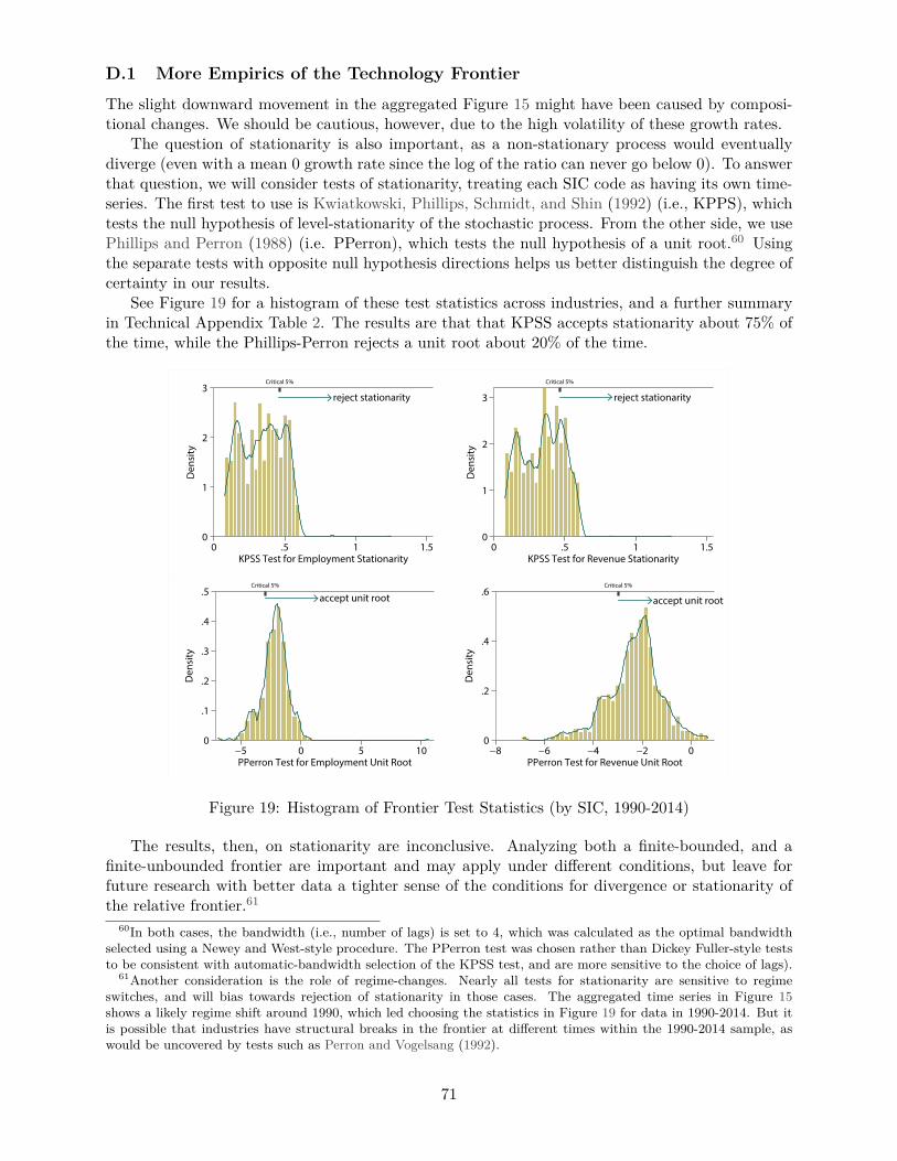
D.1 More Empirics of the Technology Frontier

The slight downward movement in the aggregated Figure 15 might have been caused by composi-tional changes. We should be cautious, however, due to the high volatility of these growth rates.

The question of stationarity is also important, as a non-stationary process would eventuallydiverge (even with a mean 0 growth rate since the log of the ratio can never go below 0). To answerthat question, we will consider tests of stationarity, treating each SIC code as having its own time-series. The first test to use is Kwiatkowski, Phillips, Schmidt, and Shin (1992) (i.e., KPPS), whichtests the null hypothesis of level-stationarity of the stochastic process. From the other side, we usePhillips and Perron (1988) (i.e. PPerron), which tests the null hypothesis of a unit root.60 Usingthe separate tests with opposite null hypothesis directions helps us better distinguish the degree ofcertainty in our results.

See Figure 19 for a histogram of these test statistics across industries, and a further summaryin Technical Appendix Table 2. The results are that that KPSS accepts stationarity about 75% ofthe time, while the Phillips-Perron rejects a unit root about 20% of the time.

0

1

2

3

De

nsi

ty

Critical 5%

0 .5 1 1.5KPSS Test for Employment Stationarity

0

1

2

3

De

nsi

ty

Critical 5%

0 .5 1 1.5KPSS Test for Revenue Stationarity

0

.1

.2

.3

.4

.5

De

nsi

ty

Critical 5%

−5 0 5 10PPerron Test for Employment Unit Root

0

.2

.4

.6

De

nsi

ty

Critical 5%

−8 −6 −4 −2 0PPerron Test for Revenue Unit Root

reject stationarity reject stationarity

accept unit root accept unit root

Figure 19: Histogram of Frontier Test Statistics (by SIC, 1990-2014)

The results, then, on stationarity are inconclusive. Analyzing both a finite-bounded, and afinite-unbounded frontier are important and may apply under different conditions, but leave forfuture research with better data a tighter sense of the conditions for divergence or stationarity ofthe relative frontier.61

60In both cases, the bandwidth (i.e., number of lags) is set to 4, which was calculated as the optimal bandwidthselected using a Newey and West-style procedure. The PPerron test was chosen rather than Dickey Fuller-style teststo be consistent with automatic-bandwidth selection of the KPSS test, and are more sensitive to the choice of lags).

61Another consideration is the role of regime-changes. Nearly all tests for stationarity are sensitive to regimeswitches, and will bias towards rejection of stationarity in those cases. The aggregated time series in Figure 15shows a likely regime shift around 1990, which led choosing the statistics in Figure 19 for data in 1990-2014. But itis possible that industries have structural breaks in the frontier at different times within the 1990-2014 sample, aswould be uncovered by tests such as Perron and Vogelsang (1992).

71

D.2 Transition Probabilities

The parameters for the transition rates are roughly calibrated from growth rates of firms in Com-pustat. While this data source has significant selection issues, this is less of an issue for calibratinggrowth rates and transitions (since our theory says that R&D based growth for incumbents is drivenby the upper tail of the distribution).

The data comes from Compustat from 1971-2014, for all firms with primary SIC 2000-3999.We can use a longer-panel than the proxies for the frontier, since individual firm growth rates arenot sensitive to the bias on the calculation of percentiles with small samples. The demeaned yearlygrowth rate in real revenue is calculated for each firm. Any firms with a growth rate > .05 areassigned the high type, and others are assigned the low type.

Note that the transition matrix P for t years is etP . From the data, at yearly frequency, thetransition matrix of the changes in types is calculated and equated

exp(

1.0×[−λ` λ`λh −λh

])=[0.74 0.260.55 0.45

]

The solution to this system of equations is λ` = 0.533074 and λh = 1.12766. While the transitionprobabilities themselves are sensitive to the thresholds for choosing ` vs. h types, this has littleimpact on the equilibrium itself.

D.3 Tail Parameters

When looking at a more realistic model with product differentiation, Technical Appendix (G.24)shows how higher markups lead to changes in the tail parameter of the size distribution, α, com-pared to the underlying productivity distribution. With the α generated by the model, TechnicalAppendix (G.30) shows a rough adjustment of α = ($ − 1)α is necessary to compare to the tailparameter in the data, where $ is the elasticity of substitution. If $ = 3, as in Perla, Tonetti, andWaugh (2015), then markups are 50%, and an α = 2.12 corresponds to the α = 1.06 tail parameterin the size or profits distribution—as used in Luttmer (2007)

D.4 Bargaining Power

From Kemmerer and Lu (2012), the reported royalty rates (i.e., the proportion of profits a licensormust pay for the intellectual property) from a data source called RoyaltySource are heterogeneousbetween industries, ranging between roughly 4% and 13%, with a median royalty rate of 5%.

In our model, from (94), the surplus going to the licensor is (1−ψ)(v`(z)−v(0)). If v`(z)� v(0),such as the adoption of a frontier technology, then this translates to a ψ = .95 to match the royaltyrate. The effective royalty rates for technologies with lower z diminish towards 0 due to the role ofthe outside option.

As we suspect that royalty rates that are actually reported are skewed towards those withenforceable IP near the frontier, we use the ψ = .95 parameter and do a robustness check to testthe sensitivity.

D.5 Frontier Productivity

The frontier productivity depends on the interpretation and selection by industry. Two approachesto consider:

TFP from Industry Studies Syverson (2011) surveys the evidence on productivity dispersion.Within the US, the ratio of the top to the bottom decile is approximately 1.92:1 . This provides a

72

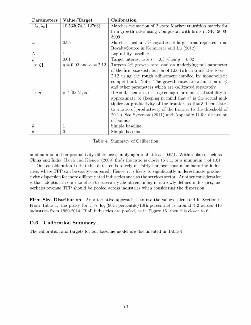
Parameters Value/Target Calibration{λ`, λh} {0.533074, 1.12766} Matches estimation of 2 state Markov transition matrix for

firm growth rates using Compustat with firms in SIC 2000-3999

ψ 0.95 Matches median 5% royalties of large firms reported fromRoyaltySource in Kemmerer and Lu (2012)

Λ 1 Log utility baselineρ 0.01 Target interest rate r = .03 when g = 0.02{χ, ζ} g = 0.02 and α = 2.12 Targets 2% growth rate, and an underlying tail parameter

of the firm size distribution of 1.06 (which translates to α =2.12 using the rough adjustment implied by monopolisticcompetition). Note: The growth rates are a function of ψand other parameters which are calibrated separately.

{z, η} z ∈ [0.651,∞] If η = 0, then z is set large enough for numerical stability toapproximate ∞ (keeping in mind that ez is the actual mul-tiplier on productivity of the frontier, so z = 3.0 translatesto a ratio of productivity of the frontier to the threshold of20.1.) See Syverson (2011) and Appendix D for discussionof bounds.

κ 1 Simple baselineθ 0 Simple baseline

Table 4: Summary of Calibration

minimum bound on productivity differences, implying a z of at least 0.651. Within places such asChina and India, Hsieh and Klenow (2009) finds the ratio is closer to 5:1, or a minimum z of 1.61.

One consideration is that this data tends to rely on fairly homogeneous manufacturing indus-tries, where TFP can be easily compared. Hence, it is likely to significantly underestimate produc-tivity dispersion for more differentiated industries such as the services sector. Another considerationis that adoption in our model isn’t necessarily about remaining in narrowly defined industries, andperhaps revenue TFP should be pooled across industries when considering the dispersion.

Firm Size Distribution An alternative approach is to use the values calculated in Section 6.From Table 1, the proxy for z ≈ log (90th percentile/10th percentile) is around 4.2 across 416industries from 1980-2014. If all industries are pooled, as in Figure 15, then z is closer to 6.

D.6 Calibration Summary

The calibration and targets for our baseline model are documented in Table 4.

73