Embed Size (px)
Citation preview
File: DISTL2 580201 . By:CV . Date:16:06:98 . Time:09:28 LOP8M. V8.B. Page 01:01Codes: 4328 Signs: 2137 . Length: 51 pic 3 pts, 216 mm
Annals of Physics�PH5802
Annals of Physics 266, 454�496 (1998)
Reconstruction of Quantum States of Spin Systems:From Quantum Bayesian Inference to
Quantum Tomography
V. Buz� ek
Optics Section, The Blackett Laboratory, Imperial College, London SW7 2BZ, England; andInstitute of Physics, Slovak Academy of Sciences, Du� bravska� cesta 9,
842 28 Bratislava, Slovakia
R. Derka
Department of Physics, Oxford University, Parks Road, Oxford OX1 3PU, England
G. Adam
Institut fu� r Theoretische Physik, Technische Universita� t Wien, Wiedner Hauptstrasse 8-10,A-1040 Vienna, Austria
and
P. L. Knight
Optics Section, The Blackett Laboratory, Imperial College, London SW7 2BZ, England
Received July 1, 1997; revised December 17, 1997
We study in detail the reconstruction of spin-1�2 states and analyze the connection between(1) quantum Bayesian inference, (2) reconstruction via the Jaynes principle of maximumentropy, and (3) complete reconstruction schemes such asdiscrete quantum tomography. Wederive an expression for a density operator estimated via Bayesian quantum inference in thelimit of an infinite number of measurements. This expression is derived under the assumptionthat the reconstructed system is in a pure state. In this case the estimation corresponds toaveraging over a microcanonical ensemble of pure states satisfying a set of constraints imposedby the measured mean values of the observables under consideration. We show that via a``purification'' ansatz, statistical mixtures can also be consistently reconstructed via the quantumBayesian inference scheme. In this case the estimation corresponds to averaging over thegeneralized grand canonical ensemble of states satisfying the given constraints, and in the limit oflarge number of measurements this density operator is equal to the generalized canonical densityoperator, which can be obtained with the help of the Jaynes principle of the maximum entropy.We also discuss inseparability of reconstructed density operators of two spins-1�2. � 1998
Academic Press
Article No. PH985802
4540003-4916�98 �25.00Copyright � 1998 by Academic PressAll rights of reproduction in any form reserved.
File: DISTL2 580202 . By:CV . Date:16:06:98 . Time:09:28 LOP8M. V8.B. Page 01:01Codes: 3861 Signs: 3374 . Length: 46 pic 0 pts, 194 mm
I. INTRODUCTION
The concept of a quantum state represents one of the most fundamental pillarsof the paradigm of quantum theory [1�3]. Contrary to its mathematical eleganceand convenience in calculations, the physical interpretation of a quantum state isnot so transparent. The problem is that the quantum state (described either by astate vector, or density operator or a phase-space probability density distribution)does not have a well defined objective status, i.e., a state vector is not an objectiveproperty of a particle. According to Peres (see [1, p. 374]), ``There is no physicalevidence whatsoever that every physical system has at every instant a well definedstate... . In strict interpretation of quantum theory these mathematical symbols [i.e.,state vectors] represent statistical information enabling us to compute the probabilitiesof occurrence of specific events.'' Once this point of view is adopted then it becomesclear that any ``measurement'' or reconstruction of a density operator (or itsmathematical equivalent) can be understood exclusively as an expression of ourknowledge about the quantum mechanical state based on a certain set of measureddata. To be more specific, any quantum-mechanical reconstruction scheme is nothingmore than an a posteriori estimation of the density operator of a quantum-mechanical(microscopic) system based on data obtained with the help of a macroscopicmeasurement apparatus [3]. The recognition of quantum-state measurement andreconstruction schemes stems from potential applications of these schemes inatomic, molecular, and condensed-matter physics, as well as quantum-informationprocessing [4].
The quality of the reconstruction depends on the ``quality'' of the measured dataand the efficiency of the reconstruction procedure with the help of which the dataanalysis is performed. In particular, we can specify three different situations. First,in the case when all system observables are precisely measured, the completereconstruction of an initially unknown state can be performed (we will call thisthe reconstruction on the complete observation level). Second, when just part ofthe system observables is precisely measured then one cannot perform a completereconstruction of the measured state. Nevertheless, the reconstruction of the densityoperator of the quantum system under consideration can be performed in thiscase with the help of the Jaynes principle of Maximum Entropy (see below). Thisreconstructed density operator uniquely determines mean values of the measuredobservables and in addition it can provide us with nontrivial estimations of unmeasuredobservables (we will denote this type of scheme as reconstruction on incompleteobservation levels). Finally, when measurement does not provide us with sufficientinformation to specify the exact mean values (or probability distributions) but onlythe frequencies of appearances of eigenstates of the measured observables, then onecan perform an estimation (reconstruction based on quantum Bayesian inference)which is the ``best'' with respect to the given measured data and the a priori knowledgeabout the state of the measured system.
The main purpose of the present paper is to demonstrate the intrinsic connectionbetween quantum Bayesian inference, incomplete quantum state reconstruction based
455RECONSTRUCTION OF QUANTUM STATES

File: DISTL2 580203 . By:CV . Date:16:06:98 . Time:09:28 LOP8M. V8.B. Page 01:01Codes: 3538 Signs: 2921 . Length: 46 pic 0 pts, 194 mm
on the MaxEnt principle and complete reconstruction of a quantum-mechanical state.We start the paper with a brief description of various reconstruction schemes andwe set up the scene for our further discussion. In Sections III and IV we review theJaynes principle of maximum entropy and the quantum Bayesian inference scheme,respectively. In Section V we present a proof that the standard Bayesian inference(developed for the reconstruction of pure states) in the limit of infinite number ofmeasurements is equivalent to an averaging over generalized microcanonical ensemblesunder the given constraints. In Section VI we show that with the help of the purificationansatz the Bayesian inference scheme can be used for the reconstruction of impurestates. In subsequent sections we concentrate our attention on the reconstruction forone and two spins-1�2 systems. In particular, in Section VII we briefly discuss areconstruction of spin states via the Jaynes MaxEnt principle. In Section VIII weillustrate how Bayesian inference works for a single spin-1�2 system when it is a prioriknown that this system is prepared in a pure state. Section IX is devoted to a statereconstruction of two spins-1�2 via quantum Bayesian inference. In Section X wepresent a systematic analysis of Bayesian reconstruction of a single spin-1�2 underthe a priori assumption that this system is prepared in a statistical mixture. Wesummarize our results in Section XI.
II. QUANTUM-STATE RECONSTRUCTION
A. Complete Observation Level
Provided that all system observables (i.e., the quorum [5, 6]) have been preciselymeasured, then the density operator of a quantum-mechanical system can becompletely reconstructed (i.e., the density operator can be uniquely determinedbased on the available data). In principle, we can consider two different schemes forreconstruction of the density operator (or, equivalently, the Wigner function) of thegiven quantum-mechanical system. The difference between these two schemes isbased on the way in which information about the quantum-mechanical system isobtained. The first type of measurement is such that on each element of the ensembleof the measured states only a single observable is measured. In the second type ofmeasurement a simultaneous measurement of conjugate observables is assumed. Wenote that in both cases we will assume ideal, i.e., unit-efficiency, measurements.
1. Quantum Tomography
When the single-observable measurement is performed, a distribution W |9)(A)for a particular observable A� of the state |�) is obtained in an unbiased way [7],i.e., W |9)(A)=|(8A | 9) | 2, where |8A) are eigenstates of the observable A� suchthat �A |8A)(8A |=1� . Here a question arises: What is the smallest number ofdistributions W |9)(A) required to determine the state uniquely? If we consider thereconstruction of the state of a harmonic oscillator, then this question is directly
456 BUZ8 EK ET AL.
File: DISTL2 580204 . By:CV . Date:16:06:98 . Time:09:28 LOP8M. V8.B. Page 01:01Codes: 3773 Signs: 3267 . Length: 46 pic 0 pts, 194 mm
related to the so-called Pauli problem [8] of the reconstruction of the wave-func-tion from distributions W |9)(q) and W |9)( p) for the position and momentum ofthe state |9) . As shown by Gale et al. [9] the knowledge of W |9)(q) and W |9)( p)is not in general sufficient for a complete reconstruction of the wave function. Incontrast, one can consider an infinite set of distributions W |9)(x%) of the rotatedquadrature x%=q cos %+ p sin %. Each distribution W |9)(x%) can be obtained froma measurement of a single observable x% , in which case a detector (filter) isprepared in an eigenstate |x%) of this observable. It has been shown by Vogel andRisken [10, 11] that, from an infinite set (in the case of the harmonic oscillator)of the measured distributions W |9)(x%) for all values of % such that [0<%�?],the Wigner function can be reconstructed uniquely via the inverse Radon transfor-mation. This scheme for reconstruction of the Wigner function (i.e., the opticalhomodyne tomography) has recently been realized experimentally by Raymer andhis co-workers [12].
Quantum-state tomography can be applied not only to optical fields but forreconstruction of other physical systems. In particular, recently Janicke and Wilkens[13] have suggested that Wigner functions of atomic waves can be tomographicallyreconstructed. Kurtsiefer et al. [14] have performed experiments in which Wignerfunctions of matter wave packets have been reconstructed. Yet another example of thetomographic reconstruction is a reconstruction of Wigner functions of vibrationalstates of trapped atomic ions theoretically described by a number of groups [15] andexperimentally measured by Leibfried et al. [16]. Vibrational motional states ofmolecules have also been reconstructed by this kind of quantum tomography byDunn et al. [17].
Leonhardt [18] has recently developed a theory of quantum tomography ofdiscrete Wigner functions describing states of quantum systems with finite-dimen-sional Hilbert spaces (for instance, angular momentum or spin). We note that theproblem of reconstruction of states of finite-dimensional systems is closely relatedto various aspects of quantum information processing, such as reading of registersof quantum computers [19]. This problem also emerges when states of atoms arereconstructed (see, for instance, [20]).
Here we stress once again, that reconstruction on the complete observation level(such as quantum tomography) is a deterministic inversion procedure which helpsus to ``rewrite'' measured data in the more convenient form of a density operator(Wigner function) of the measured state.
2. Filtering with Quantum Rulers
For the case of simultaneous measurement of two non-commuting observables(let us say q and p), it is not possible to construct a joint eigenstate of these twooperators, and therefore it is inevitable that the simultaneous measurement of twonon-commuting observables introduces additional noise (of quantum origin) intomeasured data. This noise is associated with Heisenberg's uncertainty relation andit results in a specific ``smoothing'' (equivalent to a reduction of resolution) of theoriginal Wigner function of the system under consideration (see Refs. [21] and [22]).
457RECONSTRUCTION OF QUANTUM STATES
File: DISTL2 580205 . By:CV . Date:16:06:98 . Time:09:28 LOP8M. V8.B. Page 01:01Codes: 3789 Signs: 3239 . Length: 46 pic 0 pts, 194 mm
To describe the process of simultaneous measurement of two non-commuting observ-ables, Wo� dkiewicz [23] has proposed a formalism based on an operational probabilitydensity distribution which explicitly takes into account the action of the measurementdevice modelled as a ``filter'' (quantum ruler). In particular, if the filter is considered tobe in its vacuum state then the corresponding operational probability density distribu-tions is equal to the Husimi (Q) function [21]. The Q function of optical fields has beenexperimentally measured using such an approach by Walker and Carroll [24]. Thedirect experimental measurement of the operational probability density distributionwith the filter in an arbitrary state is feasible in an 8-port experimental setup of thetype used by Noh et al. [25].
We note that propensities, and in particular Q-functions, can also be associatedwith discrete phase space and they can in principle be measured directly [26].These discrete probability distributions contain complete information about densityoperators of measured systems. Consequently, these density operators can be uniquelydetermined from the discrete-phase space propensities.
B. Reduced Observation Levels and MaxEnt Principle
As we have already indicated, it is well understood that density operators can, inprinciple, be uniquely reconstructed using either the single observable measurements(optical homodyne tomography) or the simultaneous measurement of two non-commuting observables. The completely reconstructed density operator containsinformation about all independent moments of the system operators. For example,in the case of the quantum harmonic oscillator, the knowledge of the densityoperator is equivalent to the knowledge of all moments ( (a-)m an) of the creation(a-) and annihilation (a) operators.
In many cases it turns out that the state of a harmonic oscillator is characterizedby an infinite number of independent moments ( (a-)m an) (for all m and n).Analogously, the state of a quantum system in a finite-dimensional Hilbert spacecan be characterized by a very large number of independent parameters. A completemeasurement of these moments would take an infinite time to perform. This meansthat even though the density operator can in principle be reconstructed the collectionof a complete set of experimental data points is (in principle) a never ending process.In addition the data processing and numerical reconstruction of the density operatorare time consuming. Therefore experimental realization of the reconstruction of thedensity operators for many systems can be difficult.
In practice, it is possible tomeasure just a finite number of independent momentsof the system operators, so that only a subset G� & (&=1, 2, ..., n) of observables fromthe quorum (this subset constitutes the so-called observation level [27]) is measured.In this case, when the complete information about the system is not available, oneneeds an additional criterion which would help to reconstruct (or estimate) the densityoperator uniquely. Provided mean values of all observables on the given observationlevel are measured precisely, then the density operator of the system under consideration
458 BUZ8 EK ET AL.
File: DISTL2 580206 . By:CV . Date:16:06:98 . Time:09:28 LOP8M. V8.B. Page 01:01Codes: 3724 Signs: 3323 . Length: 46 pic 0 pts, 194 mm
can be reconstructed with the help of the Jaynes principle of maximum entropy (theso-called MaxEnt principle) [27]. The MaxEnt principle provides us with a veryefficient prescription to reconstruct density operators of quantum-mechanical systemsproviding the mean values of a given set of observables are known. It works perfectlywell for systems with infinite Hilbert spaces (such as the quantum-mechanicalharmonic oscillator) as well as for systems with finite-dimensional Hilbert spaces(such as spin systems). If the observation level is composed of the quorum of theobservables (i.e., the complete observation level), then the MaxEnt principlerepresents an alternative to quantum tomography, i.e., both schemes are equallysuitable for the analysis of the tomographic data (for details see [28]). To bespecific, the observation level in this case is composed of all projectors associatedwith probability distributions of rotated quadratures. The power of the MaxEntprinciple can be appreciated in analyses of incomplete tomographic data (equiv-alent to a reconstruction of the Wigner function in a discrete phase space). Inparticular, Wiedemann [29] has performed a numerical reconstruction of theWigner function from incomplete tomographic data based on the MaxEnt principleas discussed by Buz� ek et al. [28]. Wiedemann has shown that in particular casesMaxEnt reconstruction from incomplete tomographic data can be several ordersbetter than a standard tomographic inversion. This result suggests that the MaxEntprinciple is the conceptual basis underlying incomplete tomographic reconstruction(irrespective whether this is employed in continuous or discrete phase spaces).
C. Incomplete Measurement and Bayesian Inference
It has to be stressed that the Jaynes principle of maximum entropy can beconsistently applied only when exact mean values of the measured observables areavailable. This condition implicitly assumes that an infinite number of repeatedmeasurements on different elements of the ensemble has to be performed to revealthe exact mean value of the given observable. In practice only a finite number ofmeasurements can be performed. What is obtained from these measurements is aspecific set of data indicating the number of times the eigenvalues of given observ-ables have appeared (which in the limit of an infinite number of measurementsresults in the corresponding quantum probability distributions). The question ishow to obtain the best a posteriori estimation of the density operator based on themeasured data. Helstrom [30], Holevo [31], and Jones [32] have shown that theanswer to this question can be given by the Bayesian inference method, providingit is a priori known that the quantum-mechanical state which is to be reconstructedis prepared in a pure (although unknown) state. When the purity condition isfulfilled, then the observer can systematically estimate an a posteriori probabilitydistribution in an abstract state space of the measured system. It is this probabilitydistribution (conditioned by the assumed Bayesian prior) which characterizesobserver's knowledge of the system after the measurement is performed. Using thisprobability distribution one can derive a reconstructed density operator, which
459RECONSTRUCTION OF QUANTUM STATES

File: DISTL2 580207 . By:CV . Date:16:06:98 . Time:09:28 LOP8M. V8.B. Page 01:01Codes: 3488 Signs: 2922 . Length: 46 pic 0 pts, 194 mm
however is subject to certain ambiguity associated with the choice of the cost func-tion (see Ref. [30, p. 25]). In general, depending on the choice of the cost functionone obtains different estimators (i.e., different reconstructed density operators). Inthis paper we adopt the approach advocated by Jones [32] when the estimateddensity operator is equal to the mean over all possible pure states weighted by theestimated probability distribution [see Eq. (4.4)]. We note once again that thequantum Bayesian inference has been developed for a reconstruction of pure quantummechanical states and in this sense it corresponds to an averaging over a generalizedmicrocanonical ensemble. Obviously, the mean of pure states is in general impure state.The deviation of the reconstructed density operator from pure states (measured interms of the von Neumann entropy) can then serve as a measure of the quality ofthe reconstruction.
In a real situation one can never design a state-preparation device to produce anensemble of identical pure states. What usually happens is that the ensemble consistsof a set of pure states, each of which is represented in the ensemble with a certainprobability (alternatively, we can say that the system under consideration isentangled with other quantum-mechanical systems). So now the question is how touse the Bayesian reconstruction scheme when the quantum-mechanical systemunder consideration is in an impure state (i.e., a statistical mixture). To apply theBayesian inference scheme, one has to define precisely three concepts: (1) theabstract state space of the measured system; (2) the corresponding invariantintegration measure of this space; and (3) the prior (i.e., the a priori knownprobability distribution on the given parametric state space). Once these objects arespecified one can estimate an a posteriori probability distribution on the state spaceafter each individual outcome of the measurement has been registered. Using thisdistribution the reconstructed density operator can be derived as an average overall state space.
III. JAYNES PRINCIPLE OF MAXIMUM ENTROPY
From a mathematical point of view any quantum state is an element \ of amanifold [\ # L(H); \-=\, Tr( \)=1] of Hermitian operators acting on the Hilbertspace H with a trace equal to unity. This manifold is a convex space in which extremepoints (i.e., pure states) play an exceptional role. Namely, each element of the manifoldcan be expressed as a convex linear combination of these extreme points. With eachquantum state \ an infinite number of macroscopic quantities (O� i) (i.e., meanvalues of observables O� i) are associated. These mean values are defined via a linearfunctional
(O� i) =Tr(O� i \). (3.1)
Pure states have also another exclusive property that, Tr( \k)=1, k # Z. Consequently,there exists an observable (at least as a Hermitian operator) which acquires in this
460 BUZ8 EK ET AL.
File: DISTL2 580208 . By:CV . Date:16:06:98 . Time:09:28 LOP8M. V8.B. Page 01:01Codes: 3248 Signs: 2567 . Length: 46 pic 0 pts, 194 mm
state an exact mean value, with a zero dispersion. Purity of quantum states can alsobe quantified with the help of the von Neumann entropy [7]
S[ \]=&Tr( \ ln \). (3.2)
The von Neumann entropy is a positive functional which has many appealingproperties such as concavity, continuity, additivity, and monotonicity (see [33]).This entropy provides us with an effective measure of the deviation of a quantumstate from a pure state (for pure states S[ \]=0).
We have already noticed that complete information about a pure state can, inprinciple, be obtained via the measurement of the single observable. However, ingeneral, this observable is not known a priori (we note that for statistical mixturesit does not exist at all). Therefore a determination (equivalent to a reconstructionor an a posteriori estimation) of a quantum state is in general based on a measurementof the mean values [see Eq. (3.1)] of a specific set of observables O� i , i=1, ..., n. Thisset of observables specifies the so called observation level O [27, 28]. If the chosenobservation level is incomplete, that is, if the density operator cannot be reconstructeduniquely from the measured mean values, then one should expect that there will be anumber of density operators which fulfill the constraints given by Eq. (3.1). In this caseone needs an additional criterion which would help to determine the reconstructeddensity operator uniquely. We note that if the pure state is incompletely reconstructedon a given observation level then the corresponding von Neumann entropy of thereconstructed state is larger than zero. According to Jaynes [27] this density operatormust be the one which fulfills the constraints (3.1) and which in addition maximizes theVon Neumann entropy Eq. (3.2) (this is the so-called MaxEnt principle). In otherwords, an a posteriori estimation (reconstruction) of the density operator based on ameasurement of a given set of observables is the most conservative assignment inthe sense that it does not permit one to draw any conclusions not warranted by thedata [34].
With the help of the MaxEnt principle one can reconstruct the density operatoron a specific observation level O. Following Jaynes [27] one can perform a reconstruc-tion procedure in three steps:
(1) Firstly, for given observation level the generalized partition function
ZO=Tr _exp \&:i
*iO� i+& , (3.3)
as a function of Lagrange multipliers *i has to be specified.
(2) Then the system of algebraic equations for the unknown *i ,
(O� i) =Tr(O� i \O)=&�
�* iln ZO(*1 , ..., *n), (3.4)
461RECONSTRUCTION OF QUANTUM STATES
File: DISTL2 580209 . By:CV . Date:16:06:98 . Time:09:28 LOP8M. V8.B. Page 01:01Codes: 3105 Signs: 2375 . Length: 46 pic 0 pts, 194 mm
has to be solved. This system of algebraic equations corresponds to the constraintsimposed by the measured mean values Eq. (3.1)
(3) Finally, the so-called generalized canonical density operator (i.e., thereconstructed density operator on a given observation level)
\O=1
ZO _exp \&:i
*i O� i+& . (3.5)
can be obtained, where *i are the solutions of Eqs. (3.4).It is important to understand that in the reconstruction scheme via the MaxEnt
principle, no a priori information about the state of the measured system is assumed.In other words, the reconstruction is performed on the most general state space of bothpure and impure states of the system.
We stress here that the exact mean value of an arbitrary observable can only beobtained when a very large (in principle, infinite) number of measurements onindividual elements of an ensemble is performed. On the other hand, it is a verylegitimate question to ask ``What is the best a posteriori estimation of a quantumstate when a measurement is performed on a finite (arbitrarily small) number ofelements of the ensemble?'' To estimate the state of the system based on an incom-plete set of data, one has to utilize more powerful estimation schemes such as thequantum Bayesian inference.
IV. QUANTUM BAYESIAN INFERENCE
The general idea of the Bayesian reconstruction scheme is based on manipulationswith probability distributions in parametric state spaces 0 and A of the measuredsystem and the measuring apparatus, respectively. The quantum Bayesian method asdiscussed in the literature [30�32] is based on the assumption that the reconstructedsystem is in a pure state described by a state vector |9), or equivalently by a pure-statedensity operator \=|9)(9 |. The manifold of all pure states is a continuum which wedenote as 0. The state space A of reading states of a measuring apparatus will befor the purpose of this paper associated with a discrete set of states.
In our case, when the standard Von Neumann measurement is considered, theapparatus states are intrinsically related to the set of mutually orthogonal projectorsP� *i , O� associated with the spectrum of a given observable O� (where *i are the corre-sponding eigenvalues).
The Bayesian reconstruction scheme is formulated as a three-step inversionprocedure:
(1) As a result of a measurement a conditional probability
p(O� , *i | \)=Tr(P� *i , O� \), (4.1)
462 BUZ8 EK ET AL.
File: DISTL2 580210 . By:CV . Date:16:06:98 . Time:09:28 LOP8M. V8.B. Page 01:01Codes: 3598 Signs: 2653 . Length: 46 pic 0 pts, 194 mm
on the discrete space A is obtained. This conditional probability distribution specifiesthe probability of finding the result *i if the measured system is in a particular state \.
(2) To perform the second step of the inversion procedure we have to specifyan a priori distribution p0( \) defined on the space 0. This distribution describes ourinitial knowledge concerning the measured system. Using the conditional probabilitydistribution p(O� , *i | \) and the a priori distribution p0( \) we can define the jointprobability distribution p(O� , *i ; \),
p(O� , *i ; \)= p(O� , *i | \) p0( \), (4.2)
on the space 0�A. We note that if no initial information about the measuredsystem is known, then the prior p0( \) has to be assumed to be constant (thisassumption is related to the Laplace principle of indifference [34]).
(3) The final step of the Bayesian reconstruction is based on the well-knownBayes rule p(x | y) p( y)=p(x; y)= p( y | x) p(x), with the help of which we find theconditional probability p( \ | O� , *i) on the state space 0,
p( \ | O� , *i)=p(O� , *i , \)
�0 p(O� , * i , \) d0, (4.3)
from which the reconstructed density operator can be obtained [see Eq. (4.4)].In the case of the repeated N-trial measurement, the reconstruction scheme
consists of an iterative utilization of the three-step procedure as described above.After the N th measurement we use as an input for the prior distribution the condi-tional probability distribution given by the output of the (N&1)st measurement.However, we can equivalently define the N-trial measurement conditional probabilityp([ ]N | \)=>N
i=1 p(O� i , * j | \) and applying the three-step procedure just once toobtain the reconstructed density operator
\([ ]N)=�0 p( \ | [ ]N) \ d0
�0 p( \ | [ ]N) d0, (4.4)
where \ in the r.h.s. of Eq. (4.4) is a properly parameterized density operator in thestate space 0.
At this point we should mention one essential problem in the Bayesian reconstruc-tion scheme, which is the determination of the integration measure d0 . The integrationmeasure has to be invariant under unitary transformations in the space 0. Thisrequirement uniquely determines the form of the measure. However, this is nolonger valid when 0 is considered to be a space of mixed states formed by allconvex combinations of elements of the original pure state space 0. Although theBayesian procedure itself does not require any special conditions imposed on thespace 0, the ambiguity in determination of the integration measure is the mainobstacle in generalization of the Bayesian inference scheme for reconstruction of apriori impure quantum states. We will show in Section VI that this problem can be
463RECONSTRUCTION OF QUANTUM STATES
File: DISTL2 580211 . By:CV . Date:16:06:98 . Time:09:28 LOP8M. V8.B. Page 01:01Codes: 2862 Signs: 1654 . Length: 46 pic 0 pts, 194 mm
solved with the help of a purification ansatz. We will also discuss in detail how toapply the quantum Bayesian inference for a reconstruction of states of a spin-1�2when just a finite number of elements of an ensemble have been measured. Beforewe do this, in the following Section we will analyze the limit of a large number ofmeasurements.
V. BAYESIAN INFERENCE IN LIMIT OF INFINITE NUMBER OFMEASUREMENTS
The explicit evaluation of an a posteriori estimation of the density operator \[ ]N
is significantly limited by technical difficulties when integration over parametricspace is performed [see Eq. (4.4)]. Even for the simplest quantum systems and fora relatively small number of measurements, the reconstruction procedure canpresent technically insurmountable problems.
On the other hand let us assume that the number of measurements of observablesO� i approaches infinity (i.e., N � �). It is clear that in this case the mean values ofall projectors (P� *j , O� i ) associated with the observables O� i are precisely known(measured): i.e.,
(P� *j , O� i) =: i
j , (5.1)
where �j : ij=1. In this case the integral on the right-hand side of Eq. (4.4) can be
significantly simplified with the help of the following lemma:
Lemma. Let us define the integral expression
I(:1 , ..., :n&1)#|1
0dx1 |
y2
0dx2 } } } |
yn&1
0dxn&1 F(x1 , ..., xn&1 | :1 , ..., :n&1), (5.2)
where
F(x1 , ..., xn&1 | :1 , ..., :n&1)=1B
x:1N1
x:2 N2
} } } x:n&1 Nn&1
(1&x1 } } } &xn&1):nN (5.3)
and :i satisfy condition �ni :i=1. The integration boundaries yk are given by relations:
yk=1& :k&1
j=1
xj ; k=2, ..., n&1 (5.4)
and B equals the product of Beta functions B(x, y):
B#B(an+1, an&1+1) B(an+an&1+1, an&2+2)
} } } B(an+an&1 } } } a2+1, a1+n&1). (5.5)
464 BUZ8 EK ET AL.
File: DISTL2 580212 . By:CV . Date:16:06:98 . Time:09:28 LOP8M. V8.B. Page 01:01Codes: 2654 Signs: 1558 . Length: 46 pic 0 pts, 194 mm
(i) The function F(x1 , ..., xn&1 | :1 , ..., :n&1) in the integral (5.2) is a normalizedprobability distribution in the (n&1)-dimensional volume given by integration boundaries.
(ii) For N � �, this probability distribution has the properties
(xi ) � :i (x2i ) � :2
i i=1, 2, 3, ..., n&1; (5.6)
i.e., this probability density tends to the product of delta functions:
limN � �
F(x1 , ..., xn&1 | :1 , ..., :n&1)=$(x1&:1) $(x2&:2) } } } $(xn&1&:n&1). (5.7)
Proof. Statement (i) can be derived by the successive application of the equation[see for example [35, Eqs. (3.191)]]
|u
0x&&1(u&x)+&1 dx=u++&&1B(+, &). (5.8)
Statement (ii) can be obtained as a result of straightforward calculation of limits ofcertain expressions containing Beta functions with integer-number arguments. Inour calculations we have used the identity
B(n+1, m)B(n, m)
=n
n+m, (5.9)
which is satisfied by Beta functions with integer-number arguments.
A. Conditional Density Distribution
Let us start with the expression for conditional probability distribution p([ ]N | \)for the N-trial measurement of a set of observables O� i . If we assume that thenumber of measurements of each observable O� i goes to infinity then we can write
p([ ]N � � | \)= limN � �
`i _ `
ni
j=1
Tr(P� *j , O� i\): i
jN& . (5.10)
The first product on the right-hand side (r.h.s.) of Eq. (5.10) is associated with eachmeasured observable O� i on a given observation level. The second product runs overeigenvalues ni of each observable O� i .
In what follows we formally rewrite the r.h.s. of Eq. (5.10): we insert in it a setof functions and we perform the integration
465RECONSTRUCTION OF QUANTUM STATES
File: DISTL2 580213 . By:CV . Date:16:06:98 . Time:09:28 LOP8M. V8.B. Page 01:01Codes: 3730 Signs: 2522 . Length: 46 pic 0 pts, 194 mm
p([ ]N � � | \)=`i {|
1
0dx i
1 |yi
2
0dx i
2 } } } |yi
ni&1
0dx i
n i&1 $[x i1&Tr(P� *1 , O� i
\)] } } }
_$[x ini&1&Tr(P*ni&1, O� i
\)] `ni&1
j=1
(x ij )
:ij N (1&x i
1 } } } x ini&1):i
ni N=(5.11)
In Eq. (5.12) we perform an integration over a volume determined by the integra-tion boundaries y i
k [see Eq. (5.4)], i.e., due to the condition �n ij=1
Tr(P� *j , O� i\)=1,
there is no need to perform integration from &� to �.At this point we utilize our Lemma. To be specific, first we separate in Eq. (5.11)
the term, which corresponds to the function I given by Eq. (5.2). Then we replacethis term by its limit expression (5.7). After a straightforward integration overvariables x i
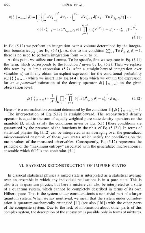
j we finally obtain an explicit expression for the conditional probabilityp( \ | [ ]N � �) which we insert into Eq. (4.4), from which we obtain the expressionfor an a posteriori estimation of the density operator \([ ]N � �) on the givenobservation level:
\([ ]N � �)=1
N |0
`i { `
ni&1
j=1
$[Tr(P� *j , O� i\)&: i
j]= \ d0 . (5.12)
Here N is a normalization constant determined by the condition Tr[ \([ ]N � �)]=1.The interpretation of Eq. (5.12) is straightforward. The reconstructed density
operator is equal to the sum of equally weighted pure-state density operators on themanifold 0, which satisfy the conditions given by Eq. (5.1) [these conditions areguaranteed by the presence of the functions in the r.h.s. of Eq. (5.12)]. In terms ofstatistical physics Eq. (5.12) can be interpreted as an averaging over the generalizedmicrocanonical ensemble of those pure states which satisfy the conditions on themean values of the measured observables. Consequently, Eq. (5.12) represents theprinciple of the ``maximum entropy'' associated with the generalized microcanonicalensemble which fullfills the constraint (5.1).
VI. BAYESIAN RECONSTRUCTION OF IMPURE STATES
In classical statistical physics a mixed state is interpreted as a statistical averageover an ensemble in which any individual realizations is in a pure state. This isalso true in quantum physics, but here a mixture can also be interpreted as a stateof a quantum system, which cannot be completely described in terms of its ownHilbert space. That is the system under considerationis a nontrivial part of a largerquantum system. When we say nontrivial, we mean that the system under consider-ation is quantum-mechanically entangled [1] (see also [36]) with the other partsof the composite system. Due to the lack of information about other parts of thiscomplex system, the description of the subsystem is possible only in terms of mixtures.
466 BUZ8 EK ET AL.

File: DISTL2 580214 . By:CV . Date:16:06:98 . Time:09:28 LOP8M. V8.B. Page 01:01Codes: 3549 Signs: 2963 . Length: 46 pic 0 pts, 194 mm
Let us assume that the quantum system P is entangled with another quantumsystemR (a reservoir). Let us assume that the composed system S (S=P�R) itselfis in a pure state |9). The density operator \P of the subsystem P is then obtainedvia tracing over the reservoir degrees of freedom:
\P=TrR [ \S]; \S=|9)(9 |. (6.1)
Once the system S is in a pure state, then we can determine an invariant integrationmeasure on the state space of the composite system S and then we can safely applythe Bayesian reconstruction scheme as described in Section IV. The reconstructionitself is based only on data associated with measurements performed on the system P.When the density operator \S is a posteriori estimated, then by tracing over thereservoir degrees of freedom, we obtain the a posteriori estimated density operator\P for the system P (with no a priori constraint on the purity of the state of thesystem P). These arguments are intrinsically related to the ``purification'' ansatz asproposed by Uhlmann [37] (see also [38]).
To make our reconstruction scheme for impure states consistent, we have tochose the reservoir R uniquely. This can be done with the help of the Schmidttheorem (see Ref. [1, 39]) from which it follows that if the composite system S isin a pure state |9) then its state vector can be written in the form
|9)= :M
i=1
ci |:i) P� |;i) R , (6.2)
where |:i) P and |; i) R are elements from two specific orthonormalized basesassociated with the subsystems P and R, respectively, and ci are appropriatecomplex numbers satisfying the normalization condition � |ci |
2=1. The maximalindex of summation (M ) in Eq. (6.2) is given by the dimensionality of the Hilbertspace of the system P. In other words, when we apply the Bayesian method to thecase of impure states of M-level system, it is sufficient to ``couple'' this system to anM-dimensional ``reservoir.'' In this case the dimensionality of the Hilbert space ofthe composite system is 2M. Using the standard techniques (see Section VIII) wecan then evaluate the invariant integration measure on the manifold of pure statesand we can apply the quantum Bayesian inference as discussed above. We stressonce again that using the purification procedure we have determined the invariantintegration measure on the space of pure states of the composite system.
We conlude this section with three comments:
(1) First, we note that there also exists another approach to the problem ofthe integration measure on thespace of impure states. Namely, Braunstein andCaves [40] used statistical distinguishability between neighboring quantum statesto define the Bures metric [41] on the space of all (pure and mixed) states of theoriginal system S (see also recent work by Slater [42]). The two approaches differconceptually in understanding what is an impure quantum-mechanical state. Thatis, in our approach we assume that impurity results as a consequence of the fact
467RECONSTRUCTION OF QUANTUM STATES
File: DISTL2 580215 . By:CV . Date:16:06:98 . Time:09:28 LOP8M. V8.B. Page 01:01Codes: 2979 Signs: 2248 . Length: 46 pic 0 pts, 194 mm
that the system under consideration is entangled with some other system. The otherapproach accepts the possiblity that an isolated quantum system can be in astatistically mixed state (we will discuss consequences of these two conceptuallydifferent approaches elsewhere).
(2) From our previous discussion it follows that for ensembles large enoughthe two reconstruction schemes provide us with the same results. Consequently,because the Bayesian inference is technically difficult to perform it is useful to utilizethe MaxEnt principle for the reconstruction in this case. On the other hand, if theensemble is small, then MaxEnt reconstruction scheme cannot be applied and thequantum Bayesian inference has to be utilized.
(3) From the results presented in Sections VI and VII it directly follows thatas soon as the number of measurements becomes large then Bayesian inferencescheme becomes equal to the reconstruction scheme based on the Jaynes principleof maximum entropy, i.e., in the limit of infinite number of measurements a posterioriestimated density operator fulfills the condition of the maximum entropy. Conse-quently, it is equal to the generalized canonical density operator. If the quorum ofobservables is measured, then the generalized canonical operator is equal to the``true'' density operator of the system itself, i.e., a complete reconstruction via theMaxEnt principle is performed.
VII. RECONSTRUCTION OF SPIN-1�2 STATES VIATHE MaxEnt PRINCIPLE
In this section we present the reconstruction of the state of a single and two spin-1�2 particles. Even though the MaxEnt reconstruction scenario in the case of asingle spin-1�2 is very simple we will use this example for a detailed illustration ofcalculation techniques which will be later used for the reconstruction of two-spin-1�2 states.
A. Single Spin-1�2
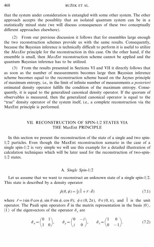
Let us assume that we want to reconstruct an unknown state of a single spin-1�2.This state is described by a density operator
\(%, ,)= 12 (1� +r� } _�^ ) (7.1)
where r� =(sin % cos ,, sin % sin ,, cos %); , # (0, 2?), % # (0, ?), and 1� is the unitoperator. The Pauli spin operators _� in the matrix representation in the basis |0) ,|1) of the eigenvectors of the operator _z are
_x=\01
10+ , _y=\0
i&i0 + , _z=\1
00
&1+ . (7.2)
468 BUZ8 EK ET AL.
File: DISTL2 580216 . By:CV . Date:16:06:98 . Time:09:28 LOP8M. V8.B. Page 01:01Codes: 2958 Signs: 1994 . Length: 46 pic 0 pts, 194 mm
To determine completely the unknown state (7.1) of a single spin-1�2 particle wehave to measure three linearly independent (e.g., orthogonal) projections of thespin. One possible choice of the complete set of observables (i.e., the quorum [5])associated with the spin-1�2 are spin projections for three orthogonal directionsrepresented by the Hermitian operators:
si#_i
2, i=x, y, z (7.3)
After the measurement of expectation values of each observable, a reconstructionof the generalized canonical density operator (3.5) according to the MaxEnt prin-ciple can be performed. In what follows we will consider three observation levelsdefined as O(1)
A =[sz], O (1)B =[sz , sx] and O (1)
C =[sz , sx , sy]#Ocomp [superscript ofthe observation levels indicates number of spins-1�2 under consideration].
1. Observation Level O (1)A =[sz]
On the observation level O(1)A only the mean value of the spin sz is measured. This
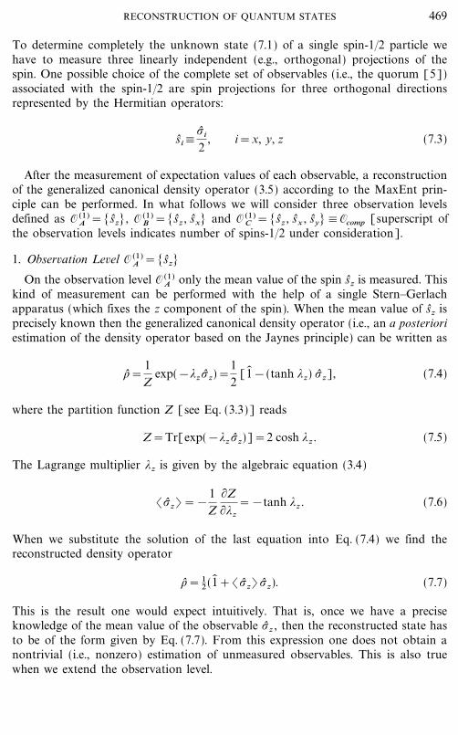
kind of measurement can be performed with the help of a single Stern�Gerlachapparatus (which fixes the z component of the spin). When the mean value of sz isprecisely known then the generalized canonical density operator (i.e., an a posterioriestimation of the density operator based on the Jaynes principle) can be written as
\=1Z
exp(&*z _z)=12
[1� &(tanh *z) _z], (7.4)
where the partition function Z [see Eq. (3.3)] reads
Z=Tr[exp(&*z _z)]=2 cosh *z . (7.5)
The Lagrange multiplier *z is given by the algebraic equation (3.4)
(_z) =&1Z
�Z�*z
=&tanh *z . (7.6)
When we substitute the solution of the last equation into Eq. (7.4) we find thereconstructed density operator
\= 12 (1� +(_z) _z). (7.7)
This is the result one would expect intuitively. That is, once we have a preciseknowledge of the mean value of the observable _z , then the reconstructed state hasto be of the form given by Eq. (7.7). From this expression one does not obtain anontrivial (i.e., nonzero) estimation of unmeasured observables. This is also truewhen we extend the observation level.
469RECONSTRUCTION OF QUANTUM STATES
File: DISTL2 580217 . By:CV . Date:16:06:98 . Time:09:28 LOP8M. V8.B. Page 01:01Codes: 3163 Signs: 1748 . Length: 46 pic 0 pts, 194 mm
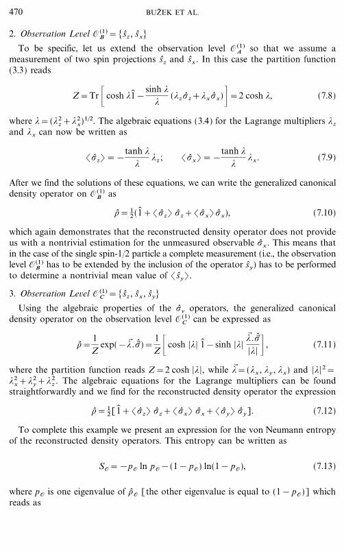
2. Observation Level O (1)B =[sz , sx]
To be specific, let us extend the observation level O(1)A so that we assume a
measurement of two spin projections sz and sx . In this case the partition function(3.3) reads
Z=Tr _cosh *1� &sinh *
*(*z _z+*x _x)&=2 cosh *, (7.8)
where *=(*2z+*2
x)1�2. The algebraic equations (3.4) for the Lagrange multipliers *z
and *x can now be written as
(_z) =&tanh *
**z ; (_x) =&
tanh **
*x . (7.9)
After we find the solutions of these equations, we can write the generalized canonicaldensity operator on O (1)
B as
\= 12 (1� +(_z) _z+(_x) _x), (7.10)
which again demonstrates that the reconstructed density operator does not provideus with a nontrivial estimation for the unmeasured observable _x . This means thatin the case of the single spin-1�2 particle a complete measurement (i.e., the observationlevel O(1)
B has to be extended by the inclusion of the operator sy) has to be performedto determine a nontrivial mean value of (sy).
3. Observation Level O (1)C =[sz , sx , sy]
Using the algebraic properties of the _& operators, the generalized canonicaldensity operator on the observation level O (1)
C can be expressed as
\=1Z
exp(&*9 ._�^ )=1Z _cosh |*| 1� &sinh |*|
*9 ._�^
|*| & , (7.11)
where the partition function reads Z=2 cosh |*|, while *9 =(*x , *y , *x) and |*|2=*2
x+*2y+*2
z . The algebraic equations for the Lagrange multipliers can be foundstraightforwardly and we find for the reconstructed density operator the expression
\= 12[1� +(_z) _z+(_x) _x+(_y) _y]. (7.12)
To complete this example we present an expression for the von Neumann entropyof the reconstructed density operators. This entropy can be written as
SO=&pO ln pO&(1& pO) ln(1& pO), (7.13)
where pO is one eigenvalue of \O [the other eigenvalue is equal to (1& pO)] whichreads as
470 BUZ8 EK ET AL.
File: DISTL2 580218 . By:CV . Date:16:06:98 . Time:09:28 LOP8M. V8.B. Page 01:01Codes: 3062 Signs: 1972 . Length: 46 pic 0 pts, 194 mm
pA=1+|(_z) |
2, pB=
1+- (_x) 2+(_z) 2
2,
(7.14)
pcomp=1+- (_x) 2+(_y) 2+(_z) 2
2.
We stress here that the reconstruction scheme based on the MaxEnt principle isperfectly well suitable for a reconstruction of both pure states and statistical mixtures;i.e., the entropy on the complete observation level can be larger then zero. That is, themeasured mean values of spin observables may be such that
(_x) 2+(_y)2+(_z) 2<1, (7.15)
which is in a striking contrast with the Bayesian quantum inference scheme [32]in which it is a priori assumed that the reconstructed state has to be a pure one,which means that on the complete observation level the condition
(_x) 2+(_y) 2+(_z) 2=1 (7.16)
has to be fulfilled, as otherwise the reconstruction scheme fails.
B. Two Spins-1�2
Let us now consider a system composed of two distinguishable spins-1�2. Ingeneral, any density operator of the system composed of two distinguishable spins-1�2 can be represented by a 4_4 Hermitian matrix and 15 independent numbersare required for its complete determination. The quorum of observables for a systemof two spins-1�2 is given by 15 operators:
s(1)i =
_i�1�
2; s (2)
i =1� � _ i
2; s (1)
i s (2)j =
_i� _j
4i, j=x, y, z. (7.17)
These operators together with the identity operator 1� �1� form the basis of operatoralgebra in which any operator associated with the system under consideration canbe expressed. In Eq. (7.17) we use the notation such that the operators which standleft (right) to the symbol � are associated with the first (second) spin-1�2.
Using the maximum-entropy principle we can (partially) reconstruct an unknowndensity operator \ on various observation levels associated with observables givenby Eq. (7.17). In what follows we will consider three observation levels.
1. Observation Level O (2)A =[s (1)
z , s (2)z ]
Let us assume a reconstruction of a quantum state of the two spins-1�2 systemwhen the observation level is given by two observables [see Eq. (7.17)] s (1)
z and s (2)z
471RECONSTRUCTION OF QUANTUM STATES
File: DISTL2 580219 . By:CV . Date:16:06:98 . Time:09:28 LOP8M. V8.B. Page 01:01Codes: 3381 Signs: 1833 . Length: 46 pic 0 pts, 194 mm
related to the first and to the second spin, respectively. Due to the fact that observ-ables associated with the first spin commute with the observables of the second spinwe can express the partition function (3.3) in a factorized form of two exponentialsassociated with each spin separately. Therefore the partition sum reads
Z=Tr[exp(&*1 _z�1� &*21� � _z)]=4 cosh *1 cosh *2 . (7.18)
The set of algebraic equations (3.4) now separates, and the resulting densityoperator can be expressed as a product of two density operators
\=1Z
[(cosh *11� &sinh *1 _z)�1� ][(1� � (cosh *21� &sinh *2 _z)]
=14
[1� �1� +(_ (1)z ) _z�1� +(_ (2)
z ) 1� � _z+(_ (1)z )(_ (2)
z ) _z� _z]
=12
[1� +(_ (1)z ) _z]�
12
[1� +(_ (2)z ) _z]. (7.19)
Here we use the notation such that (_(1)z ) , (_ (2)
z ) , and (_ (1)z _ (2)
z ) describe themean values of operators (_z �1� ) , (1� � _z) , and (_z� _z) , respectively.
2. Observation Level O (2)B =[s (1)
z , sz� sz]
Let us assume an observation level given by operators s (1)z and s (1)
z s (2)z . These
operators also commute and therefore the partition function Z can be expressed as
Z=Tr[([cosh *11� &sinh *1 _z]�1� )(cosh *121� �1� &sinh *12 _z� _z)]
=4 cosh *1 cosh *12 (7.20)
The corresponding Lagrange multipliers *1 , *12 can be found straightforwardly andwe obtain the reconstructed density matrix
\= 14[1� �1� +(_ (1)
z ) _z�1� +(_ (1)z )(_ (1)
z _ (2)z ) 1� � _z+(_ (1)
z _ (2)z ) _z � _z].
(7.21)
We point out that in this particular example the Jaynes principle of maximumentropy provides us with a nontrivial estimation for an unmeasured mean value ofthe observable _ (2)
z . The a posteriori estimation of (_ (2)z ) is equal to (_ (1)
z )(_(1)z _ (2)
z ).
3. Observation Level O (2)C =[s (1)
z , s (2)z , sz� sz]
Finally we assume the observation level when the spin projections s (1)z , s (2)
z aswell as the correlation s (1)
z s (2)z between them is measured. All these operators
472 BUZ8 EK ET AL.

File: DISTL2 580220 . By:CV . Date:16:06:98 . Time:09:28 LOP8M. V8.B. Page 01:01Codes: 3438 Signs: 2297 . Length: 46 pic 0 pts, 194 mm
mutually commute and so the partition function can be expressed as a product ofthree independent terms
Z=Tr[([cosh *1 1� &sinh *1 _z]�1� )(1� �[cosh *21� &sinh *2 _z])
_(cosh *121� �1� &sinh *12 _z� _z)], (7.22)
from which we find
Z=4[cosh *1 cosh *2 cosh *12&sinh *1 sinh *2 sinh *12 ]. (7.23)
The Lagrange multipliers have to be found from the set of algebraic equations
(_ (1)z ) =4[cosh *1 sinh *2 sinh *12&sinh *1 cosh *2 cosh *12]�Z
(_ (2)z ) =4[sinh *1 cosh *2 sinh *12&cosh *1 sinh *2 cosh *12]�Z (7.24)
(_ (1)z _ (2)
z ) =4[sinh *1 sinh *2 cosh *12&cosh *1 cosh *2 sinh *12]�Z.
Having solved these equations the reconstructed density operator reads
\= 14[1� �1� +(_ (1)
z ) _z�1� +(_ (2)z ) 1� � _z+(_ (1)
z _ (2)z ) _z� _z]. (7.25)
For further discussion on the reconstruction of spin-states via MaxEnt principlesee Ref. [43].
VIII. SPIN-1�2 RECONSTRUCTION VIA BAYESIAN INFERENCE I
In this section we study Bayesian reconstruction of spin-1�2 states on variousobservation levels. That is, we investigate how the best a posteriori estimation of thedensity operator of the spin-1�2 system based on an incomplete set of data (in thiscase the exact mean values of the spin observables are not available) can be obtained.We have already stressed the fact that the Bayesian inference scheme as introducedby Jones [32] is suitable only for pure states. This means that the completelyreconstructed density operator has to fulfill the purity condition (7.16).
We start our example with a definition of the parametric state space associatedwith the spin-1�2. The rigorous way to determine this parametric state space 0 isbased on the diffeomorphism between 0 and the quotient space SU(n)|U(n&1) , wheren is the dimensionality of the Hilbert space of the measured quantum system. In theparticular case of the spin-1�2 we work with the commutative group U(1) and theconstruction of 0 is very simple. The space 0 can be mapped on to the Poincare�sphere and the parameterized density operator (i.e., the point on the Poincare�sphere) is given by Eq. (7.1). The topology of the Poincare� sphere determines alsothe integration measure for which we have d0=sin % d% d, (for more details seeSection IX).
The observables associated with the spin-1�2 are spin projections for threeorthogonal directions represented by Hermitian operators sj given by Eq. (7.3).
473RECONSTRUCTION OF QUANTUM STATES
File: DISTL2 580221 . By:CV . Date:16:06:98 . Time:09:28 LOP8M. V8.B. Page 01:01Codes: 2839 Signs: 1789 . Length: 46 pic 0 pts, 194 mm
These observables have spectra equal to \12 . In what follows we distinguish
between these two possible measurement results by the sign, i.e., s=\1. Theprojectors P� s, si on to the corresponding eigenvectors are
P� s, si=
1� +s_i
2; i=x, y, z (8.1)
and the conditional probabilities associated with this kind of measurement can bewritten as
p(s, si | \(%, ,))=1+sri
2; i=x, y, z. (8.2)
Now using the procedure described in Section IV, we can construct an a posterioriestimation of the density operator \([ ]N) based on a given sequence of measure-ment outcomes on different observation levels.
A. Estimation Based on Results of Fictitious Measurements
In Table I we present results of an a posteriori estimation of density operatorsbased on data obtained from ``experiments'' performed with three Stern�Gerlachdevices oriented along the axes x, y, and z. We first discuss in detail reconstructionof a single spin-1�2 state under the a priori assumption that the system is in a purestate.
1. Observation Level O (1)A =[sz]
The first five lines in Table I describe results of a fictitious measurement of thespin component sz and the corresponding estimated density operators. In particular, letus assume that just one detection event (spin ``up'', i.e., A ) is registered in the givenStern�Gerlach apparatus (associated with the measurement of sz). Taking into accountthe parameterization of the single spin-1�2 density operator expressed by Eq. (7.1) wefind for the corresponding conditional probability distribution p(s, si | \(%, ,)) (8.2)the expression
p(s, si | \(%, ,))=1+cos %
2. (8.3)
Using Eq. (4.4) we can express the estimated density operator based on the registra-tion of just one result (spin ``up'') as
\=1
8? |?
0sin % d% |
2?
0d,(1+cos %)(1� +sin % cos ,_x+sin % sin ,_y+cos %_z)
=12 \1� +
13
_z+ . (8.4)
474 BUZ8 EK ET AL.
File: 595J 580222 . By:XX . Date:08:06:98 . Time:14:39 LOP8M. V8.B. Page 01:01Codes: 2794 Signs: 2199 . Length: 46 pic 0 pts, 194 mm
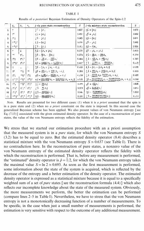
TABLE I
Results of a posteriori Bayesian Estimation of Density Operators of the Spin-1�2
Note. Results are presented for two different cases: (1) when it is a priori assumed that the spin isin a pure state and (2) when no a priori constraint on the state is imposed. In this second case thegeneralized Bayesian scheme has been applied. We also present values of von Neumann entropy [seeEq. (7.13)] associated with the given estimated density operator. In the case of a reconstruction of purestates, the value of the von Neumann entropy reflects the fidelity of the estimation.
We stress that we started our estimation procedure with an a priori assumptionthat the measured system is in a pure state, for which the von Neumann entropy S(3.2) has to be equal to zero. But the estimated density operator (8.4) describes astatistical mixture with the von Neumann entropy S&0.637 (see Table I). There isno contradiction here. In the reconstruction of pure states, a nonzero value of thevon Neumann entropy of the estimated density operator reflects the fidelity withwhich the reconstruction is performed. That is, before any measurement is performed,the ``estimated'' density operator is \=1� �2, for which the von Neumann entropy takesthe maximal value S=ln 2&0.693. As soon as the first measurement is performed,some information about the state of the system is acquired, which is reflected by thedecrease of the entropy and a better estimation of the density operator. The estimateddensity operator is expressed as a statistical mixture because it is equal to a specificallyweighted sum of a set of pure states [see the reconstruction formula (4.4)] which alsoreflects our incomplete knowledge about the state of the measured system. Obviously,the more measurements we perform, the better the estimation can be performed(compare lines 2�5 in Table I). Nevertheless, we have to stress that the von Neumannentropy is not a monotonically decreasing function of a number of measurements. Tobe specific, in the case when just a small number of measurements is performed, theestimation is very sensitive with respect to the outcome of any additional measurement.
475RECONSTRUCTION OF QUANTUM STATES
File: DISTL2 580223 . By:CV . Date:16:06:98 . Time:09:28 LOP8M. V8.B. Page 01:01Codes: 3526 Signs: 2707 . Length: 46 pic 0 pts, 194 mm
Comparing the lines 2 and 3 in Table I, we see that the entropy ``locally'' increases inspite of the fact that more measurements are performed. Nevertheless, in the limit oflarge number of measurements, the entropy approaches its minimum possible valueassociated with a given measurement. Providing the quorum of observables ismeasured, the entropy tends to zero and the state is completely reconstructed.
In general, increasing the number of measurements improves the a posterioriestimation of the density operator on the given observation level (see lines 2�5 inTable I). Using the general results of Section V we can evaluate the a posterioriestimation of the density operator of the spin-1�2 system on the observation levelO(1)
A in the limit of infinite number of measurements of the spin component sz . Wenote that in this case, when the observable has only two eigenvalues, the informa-tion obtained in the spectral distribution (5.1) is equivalently given only by themean value of this observable. Once we know the spectral distribution Eq. (5.1)corresponding to the measurement of the spin projection sz of single spin-1�2, thenwith the help of Eq. (5.12) we can express the reconstructed density operator as
\=1
N |2?
0d, |
?
0sin % d% $((_z) &cos %)
_(1� +sin % cos , _x+sin % sin , _y+cos % _z), (8.5)
where N is the normalization constant such that Tr \=1. Integration over thevariable , in Eq. (8.5) cancels all terms in front of the operators _x and _y and weobtain
\=1
N |?
0sin % d% $((_z)&cos %)(1� +cos % _z). (8.6)
The right hand side of this equation suggests a simple geometrical interpretation ofthe quantum Bayesian inference in the limit of infinite number of measurements.Namely, the density operator (8.6) can be understood as an equally weighted averageof all pure states with the same (i.e., measured) mean value of the operator sz . Thesestates are represented as points on a circle on the Poincare� sphere. When we performthe integration over % in Eq. (8.6) we obtain the final expression
\= 12 (1� +(_z) _z). (8.7)
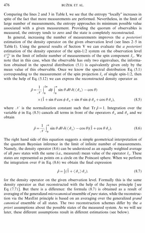
for the density operator on the given observation level. Formally this is the samedensity operator as that reconstructed with the help of the Jaynes principle [seeEq. (7.7)]. But there is a difference: the formula (8.7) is obtained as a result ofaveraging of the generalized microcanonical ensemble of pure states, while the reconstruc-tion via the MaxEnt principle is based on an averaging over the generalized grandcanonical ensemble of all states. The two reconstruction schemes differ by the apriori assumptions about the possible states of the measured system. As we will seelater, these different assumptions result in different estimations (see below).
476 BUZ8 EK ET AL.

File: DISTL2 580224 . By:CV . Date:16:06:98 . Time:09:28 LOP8M. V8.B. Page 01:01Codes: 3384 Signs: 2128 . Length: 46 pic 0 pts, 194 mm
2. Observation Level O (1)B =[sz , sx]
The results of a numerical reconstruction of the density operator of the spin-1�2based on the measurement of two spin components sz and sx are presented inTable I (lines 6�9). Lines 1�4 and 6�9 describe estimations based on the same datafor the sz measurement, but they differ in the data for the sx measurement. That is,lines 1�4 describe the situation for which no results for sx are available, while lines6�9 describe the situation with specific outcomes for the sx measurements. Comparingthese two cases (i.e., if we compare the values of the von Neumann entropy for pairsof lines [x, x+5]; x=1, 2, 3, 4) we see that any measurement performedon theadditional observable (sx) can only improve our estimation based on the measure-ment of the original observable (sz).
In the limit of infinite number of measurements, when we have information aboutthe spectral distribution corresponding to measurement of spin projections sx , sz
the particular form of Eq. (5.12) reads
\=1
N |2?
0d, |
?
0sin % d% $((_z)&cos %) $((_x)&sin % cos ,)
_(1� +sin % cos ,_x+sin % sin , _y+cos % _z). (8.8)
As seen from the right-hand side of Eq. (8.8) in this case the reconstructed densityoperator is represented by an equally weighted sum of points given by an inter-section of two circles lying on the Poincare� sphere. These two circles are specifiedby the two equations (_z) =cos % and (_x) =sin %cos ,.
With the help of the identity
$( f (x))= :x0 , f (x0)=0
$(x&x0)| f $(x0)|
, (8.9)
we can perform the integration over , in Eq. (8.8) and obtain
\=1
N |L
d% :,0
sin %|sin % sin ,0 |
$((_z)&cos %)
_(1� +(_x) _x+sin % sin ,0 _y+cos % _z). (8.10)
The integration boundaries L on the right-hand side of Eq. (8.10) are defined as
L :=0�%�? and |sin %|�|(_x) |. (8.11)
The sum on the right-hand side of Eq. (8.10) refers to two values of the parameter,0 which fulfill the condition cos ,0=(_x)�sin %. We note that the function in frontof the operator _y disappears due to the fact that it is proportional to sin ,0�|sin ,0|,which is an odd function of ,0 . After we perform the integration over % we obtain
\= 12 (1� +(_x) _x+(_z) _z). (8.12)
477RECONSTRUCTION OF QUANTUM STATES
File: DISTL2 580225 . By:CV . Date:16:06:98 . Time:09:28 LOP8M. V8.B. Page 01:01Codes: 3837 Signs: 2892 . Length: 46 pic 0 pts, 194 mm
What we see again is that in the limit of a large number of measurements the Bayesianinference formally gives us the same result as the Jaynes principle of maximum entropy[compare with Eq. (7.10)].
3. Observation Level O (1)C =[sz , sx , sy]
Further extension of the observation level O(1)B leads us to the complete observation
level, when all three spin components sx , sy and sz of the spin-1�2 are measured. Resultsof the numerical reconstruction are presented in Table I (lines 10�13). Now wecompare the a posteriori estimation of density operators based on data presented inlines 6�9. The ``experimental data'' in line 10 are equal to those presented in line 6except that now some additional knowledge concerning the spin component sy isavailable. We note that this additional information about sy improves our estima-tion of the density operator which is clearly seen when we compare values of thevon Neumann entropy presented in Table I.
Providing that we have information concerning the spectral distribution associatedwith the measurement of a complete set (i.e., the quorum) of operators sx , sy , sz (i.e.,after an infinite number of measurements of the three spin components have beenperformed), then we can express the estimated density operator as [see Eq. (5.12)]
\=1
N |2?
0d, |
?
0sin % d% $((_z) &cos %) $((_x)&sin % cos ,) $((_y)&sin % sin ,)
_(1� +sin % cos ,_x+sin % sin ,_y+cos %_z). (8.13)
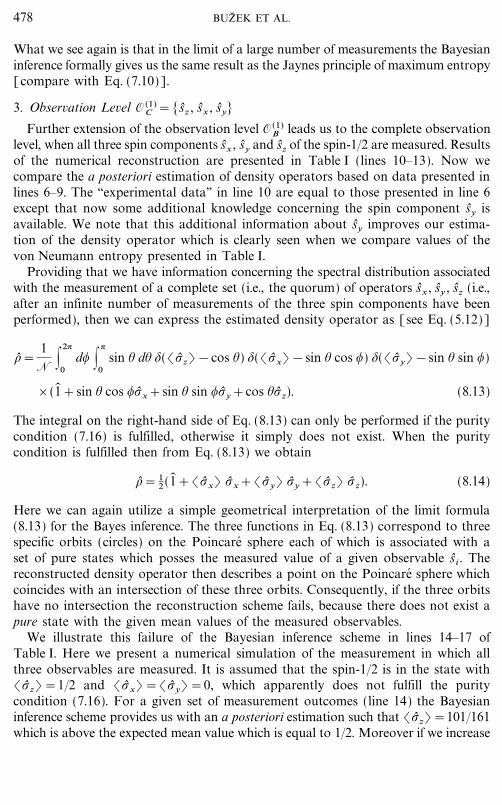
The integral on the right-hand side of Eq. (8.13) can only be performed if the puritycondition (7.16) is fulfilled, otherwise it simply does not exist. When the puritycondition is fulfilled then from Eq. (8.13) we obtain
\= 12 (1� +(_x) _x+(_y) _y+(_z) _z). (8.14)
Here we can again utilize a simple geometrical interpretation of the limit formula(8.13) for the Bayes inference. The three functions in Eq. (8.13) correspond to threespecific orbits (circles) on the Poincare� sphere each of which is associated with aset of pure states which posses the measured value of a given observable si . Thereconstructed density operator then describes a point on the Poincare� sphere whichcoincides with an intersection of these three orbits. Consequently, if the three orbitshave no intersection the reconstruction scheme fails, because there does not exist apure state with the given mean values of the measured observables.
We illustrate this failure of the Bayesian inference scheme in lines 14�17 ofTable I. Here we present a numerical simulation of the measurement in which allthree observables are measured. It is assumed that the spin-1�2 is in the state with(_z) =1�2 and (_x) =(_y) =0, which apparently does not fulfill the puritycondition (7.16). For a given set of measurement outcomes (line 14) the Bayesianinference scheme provides us with an a posteriori estimation such that (_z)=101�161which is above the expected mean value which is equal to 1�2. Moreover if we increase
478 BUZ8 EK ET AL.
File: DISTL2 580226 . By:CV . Date:16:06:98 . Time:09:28 LOP8M. V8.B. Page 01:01Codes: 3453 Signs: 2950 . Length: 46 pic 0 pts, 194 mm
the number of measurements (lines 15�17) the a posteriori estimation deviates moreand more from what would be a correct estimation (i.e., results presented in lines 14�17correspond to the following sequence of mean values of _z : 0.481; 0.375; 0.345; 0.332)but simultaneously the von Neumann entropy S decreases, which should indicate thatour estimation is better and better. This clearly illustrates the intrinsic conflict inthe estimation procedure.
The reason for this contradiction lies in the a priori assumption about the purityof the reconstructed state, i.e., the mean values of the spin components do not fulfillthe condition (7.16) and so the Bayesian method cannot be applied safely in thepresent case. The larger the number of measurement the more clearly the incon-sistency is seen and, as follows from Eq. (8.13), in the limit of infinite number ofmeasurements the Bayesian method fails completely. On the other hand the Jaynesmethod can be applied safely in this case. The point is that this method is not basedon an a priori assumption about the purity of the reconstructed state. The Jaynesprinciple is associated with maximization of entropy on the generalized grandcanonical ensemble, which means that all states (pure and impure) are taken intoaccount.
In the present example the discrepancy between the a posteriori estimations ofdensity operators based on the two different schemes has appeared only on thecomplete observation level. For more complex quantum-mechanical systems thedifference between the density operator reconstructed with the help of the Jaynesprinciple of maximum entropy and the density operator obtained via the Bayesianinference scheme may differ even on incomplete observation levels. To see this wepresent in the following sections an example of reconstruction of density operatorsdescribing states of two spins-1�2.
IX. QUANTUM BAYESIAN INFERENCE OF TWO-SPINS-1�2 STATES
In order to apply the general formalism of quantum Bayesian inference as describedin Section IV we have to properly parameterize the state space of the quantum systemunder consideration. Once this is done we have to find the invariant integrationmeasure d0 associated with the state space and only then can we effectively use thereconstruction formula (4.3). We start this section with a description of how the statespace of two spins-1�2 can be parameterized. We show how the corresponding integra-tion measure can then be found.
A. Parameterization of Two-Spins-1�2 State Space
One way to determine the state space 0 of a given quantum-mechanical system isvia a diffeomorphism 0# SU(n)|U(n&1) . This directly provides us with informationabout the dimensionality of 0, which is (dimSU(n)&dimU(n&1))=2n&2. This meansthat in our case of two spins-1�2 which are prepared in a pure state we need 6 coor-dinates which parameterize 0 (n=4). Unfortunately, it is not very convenient to
479RECONSTRUCTION OF QUANTUM STATES

File: DISTL2 580227 . By:CV . Date:16:06:98 . Time:09:28 LOP8M. V8.B. Page 01:01Codes: 3446 Signs: 1698 . Length: 46 pic 0 pts, 194 mm
determine the state space via the given diffeomorphism because then we have towork with noncommutative groups.
It is much simpler to parameterize the state space 0 utilizing the idea of theSchmidt decomposition [1]. In this case we can represent any pure state |9)describing two spins-1�2 as
|9)=A |A1) � |A2) +B |a1) � |a2) , (9.1)
where |aj) , |Aj) , are two general orthonormalized bases in H2 and A, B are twocomplex numbers satisfying the condition |A|2+|B|2=1. The correspondingdensity operator of a pure state in 0 then reads
\=|A|2 |A1)(A1| � |A2)(A2|+AB* |A1)(a1| � |A2)(a2|
+A*B |a1)(A1| � |a2)(A2|+|B|2 |a1)(a1| � |a2)(a2|. (9.2)
The projectors |Aj)(Aj | and |aj)(aj | ( j=1, 2) are given by (1� +r� ( j )_�^ | A( j )) and(1� &r� ( j )_�^ | A( j )), respectively [see Eq. (8.1)], where r� (1) and r� (2) are two arbitraryunity vectors. The operators |aj)(Aj | and their Hermitian conjugates |Aj)(aj | aredetermined as
|aj)(Aj | (1� +r� ( j)_�^ ( j )) |Aj)(aj |=(1� &r� ( j )_�^ ( j )), (9.3)
from which the relation
|Aj)(aj |=ei�j (k9 ( j )_�^ ( j)+il9 ( j )_�^ ( j )) (9.4)
follows. Here the vectors k9 ( j ) are two arbitrarily chosen unity vectors which satisfythe condition k9 ( j )=r� ( j ), and l9 ( j) are equal to vector products l9 ( j)=r� ( j )_k9 ( j ). A parti-cular choice of vectors k9 j is not important because phase factors ei�j [�j # (0, 2?)] rotatethem along all possible directions. We also note that the phase factors ei�j can be alwaysincorporated in the phase � of a complex number AB*. Using the parameterization|A|=cos(:�2) and |B|=sin(:�2) we can parameterize \ as
\(:, �, ,1 , %1 , ,2 , %2)=1� �1�
4+
r� (1) _�^ �r� (2)_�^
4+cos : _r� (1)_�^ �1�
4+
1� �r� (2)_�^
4 &+sin : cos � _k9 (1)_�^ �k9 (2)_�^
4&
l9 (1)_�^ � l9 (2)_��
4 &&sin : sin � _k9 (1)_�^ � l9 (2)_�^
4+
l9 (1)_�^ �k9 (2)_�^
4 & , (9.5)
480 BUZ8 EK ET AL.
File: DISTL2 580228 . By:CV . Date:16:06:98 . Time:09:28 LOP8M. V8.B. Page 01:01Codes: 2957 Signs: 1682 . Length: 46 pic 0 pts, 194 mm
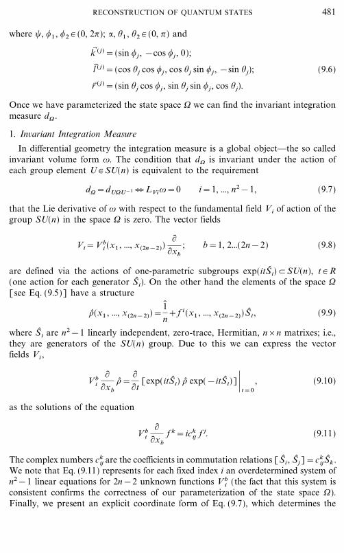
where �, ,1 , ,2 # (0, 2?); :, %1 , %2 # (0, ?) and
k9 ( j )=(sin , j , &cos ,j , 0);
l9 ( j )=(cos %j cos ,j , cos %j sin , j , &sin % j); (9.6)
r� ( j )=(sin %j cos ,j , sin % j sin , j , cos % j).
Once we have parameterized the state space 0 we can find the invariant integrationmeasure d0 .
1. Invariant Integration Measure
In differential geometry the integration measure is a global object��the so calledinvariant volume form |. The condition that d0 is invariant under the action ofeach group element U # SU(n) is equivalent to the requirement
d0=dU0U&1 � LVi |=0 i=1, ..., n2&1, (9.7)
that the Lie derivative of | with respect to the fundamental field Vi of action of thegroup SU(n) in the space 0 is zero. The vector fields
Vi=V bi (x1 , ..., x (2n&2))
��xb
; b=1, 2...(2n&2) (9.8)
are defined via the actions of one-parametric subgroups exp(itS� i)/SU(n), t # R(one action for each generator S� i). On the other hand the elements of the space 0[see Eq. (9.5)] have a structure
\(x1 , ..., x(2n&2))=1�
n+f i (x1 , ..., x (2n&2))S� i , (9.9)
where S� i are n2&1 linearly independent, zero-trace, Hermitian, n_n matrixes; i.e.,they are generators of the SU(n) group. Due to this we can express the vectorfields Vi ,
V bi
��xb
\=��t
[exp(itS� i) \ exp(&itS� i)] } t=0
, (9.10)
as the solutions of the equation
V bi
��xb
f k=ickij f j. (9.11)
The complex numbers ckij are the coefficients in commutation relations [S� i , S� j]=ck
ijS� k .We note that Eq. (9.11) represents for each fixed index i an overdetermined system ofn2&1 linear equations for 2n&2 unknown functions V b
i (the fact that this system isconsistent confirms the correctness of our parameterization of the state space 0).Finally, we present an explicit coordinate form of Eq. (9.7), which determines the
481RECONSTRUCTION OF QUANTUM STATES

File: DISTL2 580229 . By:CV . Date:16:06:98 . Time:09:28 LOP8M. V8.B. Page 01:01Codes: 2803 Signs: 1669 . Length: 46 pic 0 pts, 194 mm
invariant volume form |=m(x1 , ..., x(2n&2)) 7dx1 7 } } } 7 dx(2n&2) as the solutionof a system of partial differential equations:
��xb
(mV bi )=0. (9.12)
Here we note, that mV9 i in Eq. (9.12) has the meaning of a ``flow'' of the density ofstates generated by unitary transformations associated with the i th generator. Fromthe physical point of view Eq. (9.12) means that the divergence of this flow is zero,i.e., the number of states in each (confined) volume element is constant.
As an illustration of the above discussion we firstly evaluate the invariantmeasure for the state space of a single spin-1�2. Using Eq. (7.1) and the definition(9.11) we find the fundamental field of action Vi (i=1, 2, 3) for the three generators(7.2) of the SU(2) group:
V1=cos(,) cot(%) �,+sin(,) �% V2=sin(,) cot(%) �,&cos(,) �% V3=&�, .
(9.13)
We substitute these generators into Eq. (9.12) and after some algebra we obtain thesystem of differential equations
��,
m=0��%
m=m cot(%), (9.14)
which can be easily solved,
m(%, ,)=const sin(%). (9.15)
The multiplicative factor is given by the normalization condition. This is the routeto derive the integration measure of the Poincare� sphere. Analogously we evaluatethe invariant integration measure for a state space of two spins-1�2. The calcula-tions are technically more involved, but the result is simple:
d0=cos2 : sin : sin %1 sin %2 d: d� d,1 d%1 d,2 d%2 . (9.16)
B. Quantum Bayesian Inference of the State of Two-Spins-1�2
To perform the Bayesian reconstruction of density operators of the two-spins-1�2system we introduce a set of projectors associated with the observables (7.17)
P� s, s i(1)=
(1� +s_ i)2
�1� ; P� s, s i(2)=1� �
(1� +s_i)2
;
(9.17)
P� s, s i(1) s j
(2)=1� �1�
2+s
_ i � _j
2
482 BUZ8 EK ET AL.
File: DISTL2 580230 . By:CV . Date:16:06:98 . Time:09:28 LOP8M. V8.B. Page 01:01Codes: 3600 Signs: 2473 . Length: 46 pic 0 pts, 194 mm
The corresponding conditional probabilities can be expressed as
p(s, s (1)i | \(: } } } ))=
12
+scos(:)
2r(1)
i ; p(s, s(2)i | \(: } } } ))=
12
+scos(:)
2r(2)
i
p(s, s(1)i s(2)
j | \(: } } } ))=12
+sr(1)
i r (2)j
2(9.18)
+s sin :
2[cos �(k(1)
i k(2)j &l (1)
i l (2)j )&sin �(k(1)
i l (2)j +l (1)
i k (2)j )],
where s is the sign of the measured eigenvalue (i.e., the spectrum of observables(7.17) consists only from \1�2). Here we comment briefly on the physical meaningof the projectors defined by Eq. (9.17). Namely, the single-particle projectors of theform P� s, s i
(1) are associated with a measurement of the spin component of the firstparticle in the i-direction (i=x, y, z). Obviously this spin component can have onlytwo values, i.e., ``up'' (s=1) and ``down'' (s=&1). In Tables I and II we will denoteoutcomes of the measurements ``up'' and ``down'' as A and a, respectively. The two-particle projectors P� s, s i
(1) s j(2) are associated with measurements of correlations
between the two spin. Namely, if s=1, the two spins are correlated, which meansthat they both are registered in the same, yet unspecified, state (that is, both spinsare registered either in the state |A1A2) or |a1a2) ). In Tables I and II we willdenote this outcome of the measurement as A. On the contrary, if the particles areregistered as anticorrelated, that is, after the measurement they are in one of thetwo states |A1a2) or |a1A2) , then s=&1. In Tables I and II we will denote the out-come of this measurement for _i � _j as a.
Now we can apply general rules of Bayesian inference presented in Section IV fora two-spins-1�2 system. We will consider three specific incomplete observation levelsand we will derive asymptotic expressions for the density operators in the limit oflarge number of measurements. We stress here that we assume the measured systemto be prepared in a pure state. To be specific, let us suppose that the two spins areprepared in a state described by the state vector (obviously, this can be determinedonly after an infinite number of measurements on the complete observation level isperformed)
|9)=A |A) � |A)+B |a) � |a), (9.19)
where |A) and |a) are eigenstates corresponding to the observable of the spin projec-tion into the z-direction (i.e., (_z�1� )=(1� � _z)=|A|2&|B|2 and (_z� _z)=1).When we assume the coefficients |A| and B| to be real, then we can rewrite the densityoperator (9.19) in the form (9.5), i.e.,
\=1� �1�
4+
_z � _z
4+
A2&B2
4(_z�1� +1� �_z)+
AB2
(_x� _x&_y� _y), (9.20)
483RECONSTRUCTION OF QUANTUM STATES

File: 595J 580231 . By:XX . Date:08:06:98 . Time:14:40 LOP8M. V8.B. Page 01:01Codes: 2102 Signs: 1406 . Length: 46 pic 0 pts, 194 mm
TABLE II
Results of a posteriori Bayesian Estimation of Density Operators of the Two-Spin-1�2 System
Note. We also present explicit values of the von Neumann entropy associated with given measureddata.
with �=0, ,1=?�2, %1=0, ,2=?�2, %2=0 and sin :�2=A. In what follows weperform a posteriori estimation of the density operator based on incomplete dataobtained from three different fictitious measurement sequences.
1. Observation Level O (2)A =[s (1)
z , s (2)z ]
In the first sequence of measurements we reconstructa density operator from datawhich refer to a measurement of the first spin-1�2 in the direction z, i.e., only thespin component s (1)
z is measured (see lines 1�4 in Table II). We see that if only onespin is measured, then the reconstructed two-spin density operator can be factorized,while, as expected, the state of the unmeasured spin is estimated as \=1� �2. Obviously,in this kind of measurement, correlations between the two spins cannot be revealed, i.e.,the estimated value of _z� _z is equal to zero. As in the case of the reconstruction ofa single-spin-1�2 state, the reconstructed density operators describe statistical mixturesand the corresponding von Neumann entropy is directly related to the fidelity of thereconstruction. The maximum value of the von Neumann entropy is in the case of two-spins-1�2 equal to S=ln 4&1.386. This entropy is associated with the ``total'' mixture
484 BUZ8 EK ET AL.
File: DISTL2 580232 . By:CV . Date:16:06:98 . Time:09:28 LOP8M. V8.B. Page 01:01Codes: 3481 Signs: 2388 . Length: 46 pic 0 pts, 194 mm
of the two-spin-1�2 system and in our case it reflects a complete lack of informationabout the state of the measured system (i.e., we have no knowledge about the statebefore a measurement is performed). As soon as the first measurement is performed, wegain some knowledge about the state of the system and the entropy of the estimateddensity operator is smaller than ln 4 (see line 1 in Table II).
Let us assume now that data from the measurement of the spin components s (1)z
and s(2)z of the first and the second particle (spin-1�2), are available. In Table II
(lines 5�8) we present results of a reconstruction procedure based on the given``measured'' data. We see that though correlations between the two spins have notbeen measured directly our estimation procedure provides us with a nontrivial estima-tion for this observable (i.e., the density operator cannot be factorized). Obviously, thisestimation is affected by the prior assumption about the purity of the reconstructedstate. We see that with the increased number of detected spins the von Neumannentropy of the estimated density operator decreases (we note that it does not decreasemonotonically as a function of the number of measurements).
In the limit of large (infinite) number of measurements spectral distributionsEq. (5.1) associated with observables on a given incomplete observation level areprecisely determined by the measured data. Using the parameterization introducedearlier in this section [see Eqs. (9.5) and (9.16�9.18)] we can write down theexpression (5.12) for the Bayesian a posteriori estimation of the density operator inthe limit of large number of measurements. After we perform some trivial integra-tions and when the substitution cos :=x, cos %1= y, cos %2=z is performed we canwrite the reconstructed density operator as
\=1
N |1
&1x2 dx |
1
&1dy |
1
&1dz $((_ (1)
z )&xy) $((_ (2)z ) &xz)
_(1� �1� +xy_z �1� +xz1� � _z+yz_z� _z). (9.21)
The right-hand side of Eq. (9.21) can easily be integrated over the variables y andz so we can write
\=1
N |L
dx \1� �1� +(_ (1)z ) _z�1� +(_ (2)
z ) 1� � _z+(_ (1)
z )(_ (2)z )
x2 _z� _z+ ,
(9.22)
where the integration is performed over the interval L,
L :=[&1, 1] and |x|�smax , (9.23)
with smax=max[ |(_ (1)z ) |, |(_ (2)
z ) |]. After we perform the integration over thevariable x we find
\=14 \1� �1� +(_ (1)
z ) _z�1� +(_ (2)z ) 1� � _z+
(_ (1)z )(_ (2)
z )smax
_z � _z+ . (9.24)
485RECONSTRUCTION OF QUANTUM STATES
File: DISTL2 580233 . By:CV . Date:16:06:98 . Time:09:28 LOP8M. V8.B. Page 01:01Codes: 3630 Signs: 2788 . Length: 46 pic 0 pts, 194 mm
Comparing Eqs. (7.19) and (9.24) we see that on the observation level O (2)B the
quantum Bayesian inference and the Jaynes principle of maximum entropy providesus with the different a posteriori estimations of density operators. To be specific, thedensity operator (7.19) obtained with the help of the MaxEnt principle can beexpressed in a factorized form while the density operator (9.24) cannot be factorizedinto a product of two density operators describing each spin separately [the onlyexception is when smax=1].
2. Observation Level O (2)B =[s (1)
z , s (1)z s (2)
z ]
Here we start our discussion with an assumption that only correlations betweenthe particles are measured, while the state of each individual particle after themeasurement is unknown (see lines 9�12 in Table II). In this case we are not ableto make any nontrivial estimation for the mean values of the spin components ofthe individual particles. In order to have a better estimation we also have tomeasure at least one of the spin components of the first or the second spin.
Let us assume that the z-component of the first spin and the correlation s (1)z s (2)
z
are measured. That is, the z-component of the second spin s (2)z is not directly
observed. The question is, What is the estimation of the density operator on thisobservation level and in particular, what is the estimation for the mean value of theobservable s (2)
z ? In Table II (lines 13�16) we present numerical results for the aposteriori estimation of the density based on a finite set of ``experimental'' data. Wesee that the Bayesian scheme provides us with a nontrivial (i.e., nonzero) estimationof the mean value of s (2)
z . But the question is whether in the limit of a large numberof measurements this is equal to the mean value estimated with the help of theJaynes principle of maximum entropy. The expression for the a posteriori Bayesestimation of the density operator in the limit of infinite number of measurementson the given observation level [for technicalities see Appendix A] reads
\=14 _1� �1� +(_ (1)
z ) _z�1� +(_ (1)
z )(_ (1)z _ (2)
z )smax
1� � _z+(_ (1)z _ (2)
z ) _z � _z& ,
(9.25)
where smax=max[ |(_ (1)z ) |, |(_ (1)
z _ (2)z ) |]. Here again the Bayesian a posteriori
estimation (9.25) is in general different from the estimation (7.21)) obtained withthe help of the Jaynes MaxEnt principle. We see that these two results coincide onlywhen smax=1. For instance, if (_z� _z) =1, then smax is equal to unity and theestimated density operators given by Eqs. (7.21) and (9.25) are equal and read
\= 14[1� �1� +(_ (1)
z ) _z�1� +(_ (1)z ) 1� � _z+_z� _z]. (9.26)
In the case when (_ (1)z ) =1 the von Neumann entropy is equal to zero, i.e., the
measured state is completely reconstructed, and is described by the state vector|9)=|A1 A2).
486 BUZ8 EK ET AL.
File: DISTL2 580234 . By:CV . Date:16:06:98 . Time:09:28 LOP8M. V8.B. Page 01:01Codes: 3537 Signs: 2203 . Length: 46 pic 0 pts, 194 mm
3. Observation Level O (2)C =[s (1)
z , s (2)z , s (1)
z s (2)z ]
Finally, we will consider a measurement of both the spin projections s (1)z , s (2)
z , aswell as the correlation s (1)
z s(2)z . Results of an estimation of the density operator
based on a sequence of data associated with this observation level are given inTable II (lines 17�20). If an infinite number of measurements on the given observa-tion level is performed then we can evaluate the a posteriori density operatoranalogously to that of the previous example [see Appendix A] and after somealgebra we find
\=1
N |L"
x2
|x|dx |
z2
z1
dz$((_ (2)
z ) &xz)
- a+bz+cz2
_[1� �1� +(_ (1)z ) _z�1� +xz1� � _z+(_ (1)
z _ (2)z ) _z� _z]. (9.27)
Due to the presence of the $-function the integration over the parameter z on theright-hand side of Eq. (9.27) is straightforward and we obtain
\=1
N |L"
dx
- a+bz0+cz20
_[1� �1� +(_ (1)z ) _z�1� +(_ (2)
z ) 1� � _z+(_ (1)z _ (2)
z ) _z� _z], (9.28)
where z0=(_ (2)z )�x. From Eq. (9.28) we directly obtain the reconstructed density
operator which reads
\= 14[1� �1� +(_ (1)
z ) _z�1� +(_ (2)z ) 1� � _z+(_ (1)
z _ (2)z ) _z� _z]. (9.29)
We see that on the present observation level the density operator (9.29) estimatedvia Bayesian inference is equal to the density operator (7.25) estimated with Jaynesprinciple of maximum entropy.
C. Inseparability and Quantum Bayesian Inference
We first recall that a density operator \ab describing a system composed of twosubsystems \a and \ab is inseparable if it cannot be written as the convex sum
\ab=:m
w(m)\ (m)a � \ (m)
b . (9.30)
Inseparability is one of the most fundamental quantum phenomena, which, inparticular, may result in the violation of Bell's inequality (to be specific, a separablesystem always satisfy Bell's inequality, but the contrary is not necessarily true).Note that distant parties cannot prepare an inseparable state from a separable stateif they only use local operations and classical communications.
In the case of two spins-1�2 we can effectively utilize the Peres�Horodecki theorem[38] which states that the positivity of the partial transposition of a state is necessaryand sufficient for its separability. Before we proceed further we briefly described how
487RECONSTRUCTION OF QUANTUM STATES
File: DISTL2 580235 . By:CV . Date:16:06:98 . Time:09:28 LOP8M. V8.B. Page 01:01Codes: 3830 Signs: 2986 . Length: 46 pic 0 pts, 194 mm
to ``use'' this theorem: The density matrix associated with the density operator of twospins-1�2 can be written as
\m+, n&=(em | ( f+ | \ |en) | f&) , (9.31)
where [ |em)] ([ | f+)]) denotes an orthonormal basis in the Hilbert space of thefirst (second) spin-1�2 (for instance, |e0) =|0) a ; |e1) =|1) a , and | f0)=|0)b ;| f1)=|1) b). The partial transposition \T2 of \ is defined as
\T2m+, n&=\m&, n+ . (9.32)
Then the necessary and sufficient condition for the state \ of two spins-1�2 to beinseparable is that at least one of the eigenvalues of the partially transposedoperator (9.32) is negative.
1. Inseparability of Estimated States
To determine whether the data obtained from a incomplete measurement on agiven observation level would allow us to draw any conclusion about nonclassicalentanglement between two spins-1�2, we have to make sure that the used observa-tion level is suitable for a ``detection'' for quantum entanglement. For instance, thedensity operators reconstructed on the observation levels O (2)
A &O (2)C in the basis of
eigenstates of _z operators are diagonal. Consequently, the partially transposeddensity matrix is equal to the original density matrix. This means that all eigen-values of the partially transposed matrix are positive irrespective of the number ofmeasurements performed on these observation levels [see for instance, Eq. (9.29)].From here it follows that the given observation levels are not suitable if we wantto analyze whether the measured state is quantum-mechanically entangled. It isinteresting to note that the estimation (9.29) has been made under the assumptionthat the two-particle system is in a pure state. Obviously, there are pure two-particle states which are disentangled (i.e., |9) ab=|9) a |9) b) but all other puretwo-particle state are inseparable. But because we have chosen ``very bad'' observa-tion levels we are not able to reconstruct density operators which are inseparable.
To overcome this problem we have to extend our observation level. Namely, todetect any quantum entangled (which for instance can be seen through a violationof Bell inequalities [1]) we have to rotate the Stern�Gerlach apparatuses withwhich the measurement is performed. In particular, we can rotate them so that theprojector P� s, s x
(1) s x(2) (see Eq. (9.18) is measured. In this case the reconstructed density
operator will contain nontrivial information about the quorum of operators, i.e.,information about the mean values of the observables _x� _x and _y� _y whichwould allow us to check whether the measured state is separable.
To be specific, let us assume an extension of the observation level O (2)C =
[s (1)z , s (2)
z , s (1)z s (2)
z ] such that the operator s (1)x s (2)
x is included. We will study twoestimations of the density operator after the measurement over N (N=5, ..., 8)pairs, respectively,of two spins-1�2 is has been performed (we present results of therecontsruction in Table III). From the ``measured'' data we can estimate the
488 BUZ8 EK ET AL.
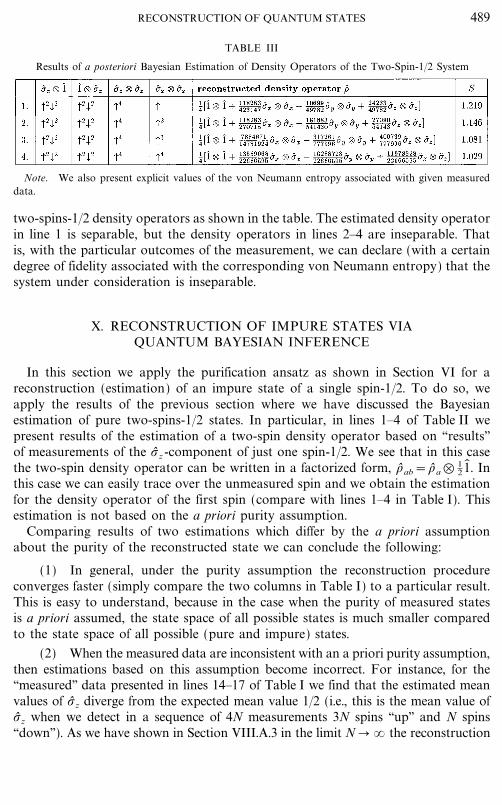
File: 595J 580236 . By:XX . Date:08:06:98 . Time:14:40 LOP8M. V8.B. Page 01:01Codes: 3198 Signs: 2507 . Length: 46 pic 0 pts, 194 mm
TABLE III
Results of a posteriori Bayesian Estimation of Density Operators of the Two-Spin-1�2 System
Note. We also present explicit values of the von Neumann entropy associated with given measureddata.
two-spins-1�2 density operators as shown in the table. The estimated density operatorin line 1 is separable, but the density operators in lines 2�4 are inseparable. Thatis, with the particular outcomes of the measurement, we can declare (with a certaindegree of fidelity associated with the corresponding von Neumann entropy) that thesystem under consideration is inseparable.
X. RECONSTRUCTION OF IMPURE STATES VIAQUANTUM BAYESIAN INFERENCE
In this section we apply the purification ansatz as shown in Section VI for areconstruction (estimation) of an impure state of a single spin-1�2. To do so, weapply the results of the previous section where we have discussed the Bayesianestimation of pure two-spins-1�2 states. In particular, in lines 1�4 of Table II wepresent results of the estimation of a two-spin density operator based on ``results''of measurements of the _z -component of just one spin-1�2. We see that in this casethe two-spin density operator can be written in a factorized form, \ab=\a� 1
2 1� . Inthis case we can easily trace over the unmeasured spin and we obtain the estimationfor the density operator of the first spin (compare with lines 1�4 in Table I). Thisestimation is not based on the a priori purity assumption.
Comparing results of two estimations which differ by the a priori assumptionabout the purity of the reconstructed state we can conclude the following:
(1) In general, under the purity assumption the reconstruction procedureconverges faster (simply compare the two columns in Table I) to a particular result.This is easy to understand, because in the case when the purity of measured statesis a priori assumed, the state space of all possible states is much smaller comparedto the state space of all possible (pure and impure) states.
(2) When the measured data are inconsistent with an a priori purity assumption,then estimations based on this assumption become incorrect. For instance, for the``measured'' data presented in lines 14�17 of Table I we find that the estimated meanvalues of _z diverge from the expected mean value 1�2 (i.e., this is the mean value of_z when we detect in a sequence of 4N measurements 3N spins ``up'' and N spins``down''). As we have shown in Section VIII.A.3 in the limit N � � the reconstruction
489RECONSTRUCTION OF QUANTUM STATES

File: DISTL2 580237 . By:CV . Date:16:06:98 . Time:09:28 LOP8M. V8.B. Page 01:01Codes: 2990 Signs: 1825 . Length: 46 pic 0 pts, 194 mm
can completely fail when the purity condition is imposed. On the other hand, if it is apriori assumed that the measured state can be in a statistical mixture, then the Bayesianquantum inference provides us with estimations which in the limit N � � coincidewith estimations based on the Jaynes principle of maximum entropy.
A. Estimation in the Limit of N � � Measurements
1. Observation Level O (1)A =[s (1)
z ]
Using the techniques which have been demonstrated in Section IX we can expressthe estimated density operator on the given observation level in the limit N � �[see Eq. (5.12)]. We note that on the considered observation level, Eq. (5.12)contains many terms, which are odd functions of the corresponding integrationvariables. Therefore the integration over these parameters (%2 , ,2 , �, ,1) is straight-forward. Moreover, if we perform the trace over the ``second'' (reservoir) spin wecan express the density operator of the spin-1�2 under consideration as
\=1
N |1
&1y2 dy |
?
0sin %1 d%1 $((_ (1)
z )& y cos %1)(1� + y cos %1 _z), (10.1)
where the variable : is substituted by y=cos :. When we perform integration overy we obtain the expression
\=2
N |L
d%1
sin %1
cos2 %1 |cos %1 |(1� +(_ (1)
z ) _z), (10.2)
with L defined as
L :=[0, ?] such that |cos %1|�|(_ (1)z ) |. (10.3)
After we perform the integration over %1 we obtain the expression for the densityoperator identical to that obtained via the Jaynes principle of maximum entropy[see Eq. (7.7)].
2. Observation Level O (1)B =[s (1)
z , s (1)x ]
In the limit of infinite number of measurements one can express the Bayesianestimation of the density operator of the spin-1�2 on the given observation level as(here the trace over the ``reservoir'' spin has already been performed)
\=1
N |1
&1y2 dy |
?
0sin %1 d%1 |
2?
0d,1 $((_ (1)
z )& y cos %1) $((_ (1)x ) & y sin %1 cos ,1)
_(1� + y sin %1 cos ,1 _x+ y sin %1 sin ,1 _y+ y cos %1 _z). (10.4)
490 BUZ8 EK ET AL.

File: DISTL2 580238 . By:CV . Date:16:06:98 . Time:09:28 LOP8M. V8.B. Page 01:01Codes: 2987 Signs: 1505 . Length: 46 pic 0 pts, 194 mm
When we perform integration over the variable y we find
\=1
N |2?
0d,1 |
L$d%1
sin %1
cos2 %1 |cos %1 |(_ (1)
x )&tan %1 cos ,1(_ (1)z ) )
_(1� +(_ (1)z ) tan %1 cos ,1 _x+(_ (1)
z ) tan %1 sin ,1 _y+(_ (1)z ) _z). (10.5)
The integration over the variable ,1 in the right-hand side of Eq. (10.5) gives us
\=1
N |L"
d%1 :2
j=1
1cos2 %1 |sin , ( j )
1 |
_(1� +(_ (1)x ) _x+(_ (1)
z ) tan %1 sin , ( j )1 _y+(_ (1)
z )_z), (10.6)
where the integration is performed over the interval
L" :=[0, ?] such that |cos %1 |�|(_ (1)z ) | , and |tan %1 |� }(_ (1)
x )(_ (1)
z ) } .(10.7)
The sum in Eq. (10.6) is performed over two values , ( j )1 of the variable ,1 which are
equal to the two solutions of the equation
cos ,1=(_ (1)
x )(_ (1)
z ) tan %1
. (10.8)
Due to the fact that the term in front of the operator _ (1)y is the odd function of , ( j )
1 ,we can straightforwardly perform in Eq. (10.6) the integration over %1 and we findthe expression of the reconstructed density operator which again is exactly the sameas if we perform the reconstruction with the help of the Jaynes principle [see Eq. (7.10)].
3. Observation Level O (1)C =[s (1)
z , s (1)x , s (1)
y ]
On the complete observation level, the expression for the Bayesian estimation ofthe density operator of the spin-1�2 in the limit of infinite number of measurementscan be expressed as (here again we have already traced over the ``reservoir'' degreesof freedoms) [see Eq. (10.4)]
\=1
N |1
&1y2 dy |
?
0sin %1 d%1 |
2?
0d,1
_$((_ (1)z ) & y cos %1) $((_ (1)
x ) & y sin %1 cos ,1) $((_ (1)y )& y sin %1 sin ,1)
_(1� + y sin %1 cos ,1 _x+ y sin %1 sin ,1 _y+ y cos %1 _z). (10.9)
491RECONSTRUCTION OF QUANTUM STATES
File: DISTL2 580239 . By:CV . Date:16:06:98 . Time:09:28 LOP8M. V8.B. Page 01:01Codes: 3166 Signs: 2220 . Length: 46 pic 0 pts, 194 mm
Performing similar calculations as in the previous subsection we can rewrite Eq. (10.9)as
\&|L"
d%1 :2
j=1
1cos2 %1 |sin , ( j )
1 |$((_ (1)
y ) &tan %1 sin , ( j )1 (_ (1)
z ) )
_(1� +(_ (1)x ) _x+(_ (1)
y ) tan %1 sin , ( j )1 _y+(_ (1)
z ) _z)�1� , (10.10)
where L" and , ( j )1 are defined by Eqs. (10.7) and (10.8), respectively. Now the
integration over %1 can be easily performed and for the density operator of thegiven spin-1�2 system we find
\= 12[1� +(_ (1)
x ) _x+(_ (1)y ) _y+(_ (1)
z ) _z], (10.11)
where the mean values (_ (1)j ) do not necessarily satisfy the purity condition (7.16).
XI. CONCLUSIONS
In the paper we have analyzed in detail the logical connection between threedifferent reconstruction schemes: (1) If measurements over a finite number ofelements of the ensemble are performed then one can obtain the a posteriori estima-tion of the density operator with the help of Bayesian inference. If nothing is knownabout the reconstructed state one has to assume a constant prior probability distri-bution on the parametric state space under the assumption that the system is in astatistical mixture. (2) As soon as the number of measurements becomes large theBayesian inference scheme becomes equal to the reconstruction scheme based onthe Jaynes principle of maximum entropy; i.e., in the limit of infinite number ofmeasurements a posteriori estimated density operator fulfills the condition of themaximum entropy. Consequently, it is equal to the generalized canonical densityoperator. (3) If the quorum of observables is measured, then the generalizedcanonical operator is equal to the ``true'' density operator of the system itself, i.e.,a complete reconstruction via the MaxEnt principle is performed. It is a matter oftechnical convenience which reconstruction scheme on the complete observationlevel is utilized (for instance, quantum tomography can be used), but all of thesecomplete reconstruction schemes can be formulated as a maximization of theentropy under given constraints.
APPENDIX
Bayesian Inference on O (2)B in the Limit of Infinite Number of Measurements
On the given observation level we can express the estimated density operator inthe limit of infinite number of measurements as [see Eq. (5.12)]
492 BUZ8 EK ET AL.

File: DISTL2 580240 . By:CV . Date:16:06:98 . Time:09:28 LOP8M. V8.B. Page 01:01Codes: 3004 Signs: 1423 . Length: 46 pic 0 pts, 194 mm
\=1
N |2?
0d� |
1
&1x2 dx |
1
&1dy |
1
&1dz
_$((_ (1)z )&xy) $((_ (1)
z _ (2)z )& yz+[(1&x2)(1& y2)(1&z2)]1�2 cos �)
_[1� �1� +xy_z�1� +xz1� � _z
+[ yz&((1&x2)(1& y2)(1&z2))1�2 cos �] _z� _z]. (A.1)
We integrate Eq. (A.1) over the variable y and we obtain
\=1
N |2?
0d� |
L$
x2
|x|dx |
1
&1dz
_$ \(_ (1)z _ (2)
z )&(_ (1)z )
zx
+_(1&x2)(1&z2) \1&(_ (1)
z ) 2
x2 +&1�2
cos �+_{1� �1� +(_ (1)
z ) _z�1� +xz1� � _z
+_(_ (1)z )
zx
&\(1&x2)(1&z2) \1&(_ (1)
z ) 2
x2 ++1�2
cos �+& _z� _z= , (A.2)
where the integration boundaries are defined as
L" :=[&1, 1] and |x|�|(_ (1)z ) |. (A.3)
Now we will integrate Eq. (A.2) over the variable �. There are two values �( j )0
( j=1, 2) of �, such that
cos �0=(_ (1)
z _ (2)z ) &(_ (1)
z ) z�x[(1&x2)(1&z2)(1&((_ (1)
z )�x)2)]1�2 , (A.4)
providing that inequality
1� } (_ (1)z _ (2)
z ) &(_ (1)z ) z�x
[(1&x2)(1&z2)(1&((_ (1)z )�x)2)]1�2 } (A.5)
holds. The last relation can be rewritten as the condition a+bz+cz2�0, where theexplicit forms of the coefficients a, b, and c are
a=1&(_ (1)z ) 2 �x2+(_ (1)
z ) 2&(_ (1)z _ (2)
z ) 2&x2 ;(A.6)
b=2(_ (1)z )(_ (1)
z _ (2)z )�x; c=x2&(_ (1)
z ) 2&1.
The coefficient c is always negative, which means that we have a new condition forthe parameter z, that is, z # (z1 , z2) , where z1 and z2 are two roots of the quadraticequation a+bz+cz2=0. However, these roots exist only providing the discrimi-nant b2&4ac�0 is nonnegative. Taking into account Eq. (A.6)we see that the lastrelation is a cubic equation with respect to the variable x2, which imposes a new
493RECONSTRUCTION OF QUANTUM STATES

File: DISTL2 580241 . By:CV . Date:16:06:98 . Time:09:28 LOP8M. V8.B. Page 01:01Codes: 4724 Signs: 2084 . Length: 46 pic 0 pts, 194 mm
condition on the integration parameter x. That is, the interval L" through whichthe integration over x in Eq. (A.2) is performed is defined as
L" :={[ |(_ (1)z ) |, 1]
[ |(_ (1)z ) |, - 1+(_ (1)
z ) 2-(_ (1)z _ (2)
z ) 2]for |(_ (1)
z _ (2)z ) |� |(_ (1)
z ) |;for |(_ (1)
z _ (2)z ) |�|(_ (1)
z ) |.
(A.7)
Taking into account all conditions imposed on parameters of integration wecanrewrite Eq. (A.2) as
\=1
N |L"
x2
|x|dx |
z2
z1
dz
- a+bz+cz2
_(1� �1� +(_ (1)z ) _z�1� +xz1� � _z+(_ (1)
z _ (2)z ) _z� _z). (A.8)
Using standard formulas [see, for example, [37, Eq. (2.261) and Eq. (2.264)]] theintegration over parameter z in Eq. (A.8) can now be performed and we obtain
\=1
N |L"
dxx2
|x|1
(1+(_ (1)z ) 2&x2)1�2 (1� �1� +(_ (1)
z ) _z�1� +(_ (1)z _ (2)
z ) _z� _z)
+|L"
dxx2
|x|(_ (1)
z )(_ (1)z _ (2)
z )(1+(_ (1)
z ) 2&x2)3�2 (1� � _z). (A.9)
After performing integration over x in Eq. (A.9) we obtain final the expression(9.25) for the a posteriori estimation of the density operator on the given observa-tion level.
ACKNOWLEDGMENTS
We thank Jason Twamley, Sam Braustein, and Zdene� k Hradil for stimulating discussions. This workwas supported in part by the United Kingdom Engineering and Physical Sciences Research Council, theEuropean Community, and the Grant Agency VEGA of the Slovak Academy of Sciences. We acknowledge thesupport by the East�West Program of the Austrian Academy of Sciences under Contract 45.367�6-IV�3a�95of the O� sterreichisches Bundesministerium fu� r Wissenschaft und Forschung.
REFERENCES
1. A. Peres, ``Quantum Theory: Concepts and Methods,'' Kluwer, Dordrecht, 1993.2. R. Omne� s, ``The Interpretation of Quantum Mechanics,'' Princeton Univ. Press, Princeton, 1994.3. L. E. Ballentine, ``Quantum Mechanics,'' Prentice Hall, Englewood Cliffs, NJ, 1990.4. See ``Quantum State Preparation and Measurement,'' special issue of J. Mod. Opt. 44, No. 11�12
(1997), edited by W. P. Schleich and M. G. Raymer.5. W. Band and J. L. Park, Amer. J. Phys. 47 (1979), 188; Found. Phys. 1 (1970), 133; Found. Phys.
1 (1971), 339; J. L. Park and W. Band, Found. Phys. 1 (1971), 211.6. R. G. Newton and Bing-Lin Young, Ann. Phys. (N.Y.) 49 (1968), 393.
494 BUZ8 EK ET AL.
File: DISTL2 580242 . By:CV . Date:16:06:98 . Time:09:28 LOP8M. V8.B. Page 01:01Codes: 8938 Signs: 4325 . Length: 46 pic 0 pts, 194 mm
7. J. von Neumann, ``Mathematical Foundations of Quantum Mechanics,'' Princeton Univ. Press,Princeton, 1955; see also J. A. Wheeler and W. H. Zurek, ``Quantum Theory and Measurement,''Princeton Univ. Press, Princeton, 1983.
8. W. Pauli, ``General Principles of Quantum Mechanics,'' Springer-Verlag, Berlin, 1980; see alsoB. d'Espagnat, ``Conceptual Foundations of Quantum Mechanics,'' 2nd ed., Benjamin, Reading,1976.
9. W. Gale, E. Guth, and G. T. Trammel, Phys. Rev. 165 (1968), 1434; see also A. Orlowski andH. Paul, Phys. Rev. 50 (1994), R921.
10. K. Vogel and H. Risken, Phys. Rev. A 40 (1989), 2847; see also J. Bertrand and P. Bertrand, Found.Phys. 17 (1987), 397; M. Freyberger, K. Vogel, and W. P. Schleich, Phys. Lett. A 176 (1993), 41;H. Ku� hn, D.-G. Welsch, and W. Vogel, J. Mod. Opt. 41 (1994), 1607; G. S. Agarwal and S. Chaturvedi,Phys. Rev. A 49 (1994), R665; W. Vogel and D.-G. Welsch, Acta Phys. Slov. 45 (1995), 313;U. Leonhardt and H. Paul, Phys. Lett. A 193 (1994), 117; U. Leonhardt and H. Paul, J. Mod. Opt.41 (1994), 1427; H. Ku� hn, D.-G. Welsch, and W. Vogel, J. Mod. Opt. 41 (1994), 1607.
11. G. M. D'Ariano, C. Machiavelo, and M. G. A. Paris, Phys. Rev. A 50 (1994), 4298; U. Leonhardt,H. Paul, and G. M. D'Ariano, Phys. Rev. A 52 (1995), 4899; G. M. D'Ariano, U. Leonhardt, andH. Paul, Phys. Rev. A 52 (1995), R1801; Th. Richter, Phys. Lett. A 211 (1996), 327; Th. Richter,Phys. Rev. A 53 (1996), 1197; U. Leonhardt, M. Munroe, T. Kiss, T. Richter, and M. G. Raymer,Opt. Commun. 127 (1996), 144.
12. D. T. Smithey, M. Beck, M. G. Raymer, and A. Faridani, Phys. Rev. Lett. 70 (1993), 1244; D. T.Smithey, M. Beck, J. Cooper, and M. G. Raymer, Phys. Scr. T 48 (1993), 35; M. Beck, M. G.Raymer, I. A. Walmsley, and V. Wong, Opt. Lett. 18 (1993), 2041; M. Beck, D. T. Smithey, andM. G. Raymer, Phys. Rev. A 48 (1993), R890; see also M. G. Raymer, M. Beck, and D. F.Mc Alister, Phys. Rev. Lett. 72 (1994), 1137; M. G. Raymer, D. T. Smithey, M. Beck, and J. Cooper,Acta Phys. Pol. 86 (1994), 71.
13. U. Janicke and M. Wilkens, J. Mod. Opt. 42 (1995), 2183.14. Ch. Kurtsiefer, T. Pfau, and J. Mlynek, in ``Technical Digest of the European Quantum Electronic
Conference,'' p. 132, Hamburg, Germany, 1996; S. Schiller, G. Breitenbach, S. F. Pereira, T. Mu� ller,and J. Mlynek, Phys. Rev. Lett. 77 (1996), 2933; Ch. Kurtsiefer, T. Pfau, and J. Mlynek, Nature 386(1997), 150.
15. S. Wallentowitz and W. Vogel, Phys. Rev. Lett. 75 (1995), 2932; J. F. Poyatos, R. Walser, J. I. Cirac,P. Zoller, and R. Blatt, Phys. Rev. A 53 (1996), R1966; C. D'Helon and G. J. Milburn, Phys. Rev.A 53 (1996), R25.
16. D. Leibfried, D. M. Meekhof, B. E. King, C. Monroe, W. M. Itano, and D. J. Wineland, Phys. Rev.Lett. 77 (1996), 4281; D. Wineland, C. Monroe, D. M. Meekhof, B. E. King, D. Liebfried, W. M.Itano, J. C. Bergquist, D. Berkeland, J. J. Bollinger, and J. Miller, ``Quantum State Manipulationof Trapped Atomic Ions,'' Los Alamos e-print archive quant-ph�9705022 (1997).
17. T. J. Dunn, I. A. Walmsley, and S. Mukamel, Phys. Rev. Lett. 74 (1995), 884.18. U. Leonhardt, Phys. Rev. Lett. 74 (1995), 4101; Phys. Rev. A 53 (1996), 2998; see also W. K. Wootters,
Found. Phys. 16 (1986), 391; W. K. Wootters, Ann. Phys. (N.Y.) 175 (1987), 1; D. Galetti andA. F. R. De Toledo Piza, Physica A 149 (1988), 267.
19. A. Barenco and A. K. Ekert, Acta Phys. Slovaca 45 (1995), 205; A. Barenco, Contemp. Phys. 37(1996), 359, and references therein.
20. R. Walser, J. I. Cirac, and P. Zoller, Phys. Rev. Lett. 77 (1996), 2658; see also A. S. Parkins,P. Marte, P. Zoller, O. Carnal, and H. J. Kimble, Phys. Rev. A 51 (1995), 1578; A. S. Parkins,P. Marte, P. Zoller, and H. J. Kimble, Phys. Rev. Lett. 71 (1993), 3095.
21. K. Husimi, Proc. Phys. Math. Soc. Jpn. 22 (1940), 264; Y. Kano, J. Math. Phys. 6 (1965), 1913.22. E. Arthurs and J. L. Kelly, Jr., Bell. Syst. Tech. J. 44 (1965), 725; W. K. Wootters and W. H. Zurek,
Phys. Rev. D 19 (1979), 473; Y. Lai and H. A. Haus, Quantum Opt. 1 (1989), 99; D. Lalovic� , D. M.Davidovic� , and N. Bijedic� , Phys. Rev. A 46 (1992), 1206; D. M. Davidovic� and D. Lalovic� , J. Phys.A 26 (1993), 5099; S. Chaturvedi, G. S. Agarwal, and V. Srinivasan, J. Phys. A 27 (1994), L39;M. G. Raymer, Amer. J. Phys. 62 (1994), 986; U. Leonhardt and H. Paul, Phys. Rev. A 48 (1993),
495RECONSTRUCTION OF QUANTUM STATES
File: DISTL2 580243 . By:CV . Date:16:06:98 . Time:09:28 LOP8M. V8.B. Page 01:01Codes: 8605 Signs: 3352 . Length: 46 pic 0 pts, 194 mm
4598; V. Buz� ek, C. H. Keitel, and P. L. Knight, Phys. Rev. A 51 (1995), 2575; see also the reviewarticles S. Stenholm, Ann. Phys. (N.Y.) 218 (1992), 233; U. Leonhardt and H. Paul, Quant. Electron.19 (1995), 89; A. Wu� nsche, and V. Buz� ek, J. Quant. Semiclass. Opt. 9 (1997), 631.
23. K. Wo� dkiewicz, Phys. Rev. Lett. 52 (1984), 1064; Phys. Lett. A 115 (1986), 304; Phys. Lett. A 129(1988), 1.
24. N. G. Walker and J. E. Carroll, Opt. Quant. Electron. 18 (1986), 335; N. G. Walker, J. Mod. Opt.34 (1987), 15.
25. J. W. Noh, A. Fouge� res, and L. Mandel, Phys. Rev. Lett. 67 (1991), 1426; Phys. Rev. A 45 (1992),424.
26. T. Opatrny� , V. Buz� ek, J. Bajer, and G. Drobny� , Phys. Rev. A 52 (1995), 2419; T. Opatrny� , D.-G.Welsch, and V. Buz� ek, Phys. Rev. A 53 (1996), 3822.
27. E. T. Jaynes, Phys. Rev. 108 (1957), 171; 620; Amer. J. Phys. 31 (1963), 66; see also E. Fick andG. Sauermann, ``The Quantum Statistics of Dynamic Processes,'' Springer-Verlag, Berlin, 1990; J. N.Kapur and H. K. Kesavan, ``Entropic Optimization Principles with Applications,'' Academic Press,New York, 1992.
28. V. Buz� ek, G. Adam, and G. Drobny� , Ann. Phys. (N.Y.) 245 (1996), 37; Phys. Rev. A 54 (1996), 801.29. H. Wiedemann, ``Quantum Tomography with the Maximum Entropy Principle,'' unpublished
manuscript.30. C. W. Helstrom, ``Quantum Detection and Estimation Theory,'' Academic Press, New York, 1976.31. A. S. Holevo, ``Probabilistic and Statistical Aspects of Quantum Theory,'' North-Holland,
Amsterdam, 1982.32. K. R. W. Jones, Ann. Phys. (N.Y.) 207 (1991), 140; Phys. Rev. A 50 (1994), 3682; see also Z. Hradil,
Phys. Rev. A 55 (1997), R1561.33. A. Wehrl, Rev. Mod. Phys. 50 (1978), 221.34. E. T. Jaynes, in ``1962 Brandeis Lectures, Vol. 3,'' (K. W. Ford, Ed.), p. 181, Benjamin, New York,
1963. Here we note, that the MaxEnt principle has a very close relation to the Laplace principle ofindifference [see, for instance, H. Jeffreys, ``Theory of Probability,'' Oxford Univ. Press., Oxford,1960] which states that where nothing is known one should choose a constant-valued function toreflect this ignorance. This obviously maximizes any uncertainty measure.
35. I. S. Gradstein and I. M. Ryzhik, ``Table of Integrals, Series, and Products,'' Academic Press, NewYork, 1980.
36. A. Peres, Phys. Rev. Lett. 77 (1996), 1413; M. Horodecki, P. Horodecki, and R. Horodecki, Phys.Lett. A 223 (1996), 1; Phys. Rev. Lett. 78 (1997), 574.
37. A. Uhlmann, Rep. Math. Phys. 9 (1976), 273; Rep. Math. Phys. 24 (1986), 229.38. R. Derka, V. Buz� ek, and G. Adam, Acta Phys. Slov. 46 (1996), 355; see also R. Derka, V. Buz� ek,
G. Adam, and P. L. Knight, J. Fine Mech. Opt. 11�12 (1996), 341.39. A. K. Ekert and P. L. Knight, Amer. J. Phys. 63 (1995), 415.40. S. L. Braunstein and C. M. Caves, Phys. Rev. Lett. 72 (1994), 3439; see also S. L. Braunstein and
C. M. Caves, Ann. New York Acad. Sci. 755 (1995), 798; S. L. Braunstein, Phys. Lett. A 219 (1996),169.
41. D. Bures, trans. Am. Math. Soc. 135 (1969), 199; M. Hu� bner, Phys. Lett. A 163 (1992), 239; Phys.Lett. A 179 (1993), 226; J. Twamley, J. Phys. A 29 (1996), 3723.
42. P. B. Slater, Physica A 214 (1995), 584; P. B. Slater, ``Noninformative Priors for QuantumInference,'' Los Alamos e-print archive quant-ph�9703012.
43. V. Buz� ek, G. Drobny� , G. Adam, R. Derka, and P. L. Knight, J. Mod. Opt. 44 (1997), 2607.
� � � � � � � � � �
496 BUZ8 EK ET AL.