Embed Size (px)
Citation preview
Recovering High Dimensional Non-Rigid Deformations Through Point Matching
Haili Chui
Image Processing and Analysis GroupDepartments of Electrical Engineering
Yale University
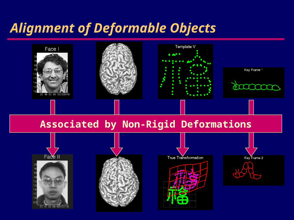
Alignment of Deformable Objects
Associated by Non-Rigid Deformations
Point Matching
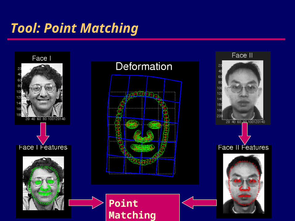
Tool: Point Matching

Outline
• Non-rigid point matching:– Problem.– Algorithm.– Search and match strategy.– Global-to-local search strategy.– Examples.
• Applications:– Key-frame animation.– Face matching/warping.
– Average shape estimation.– Brain MRI image registration.
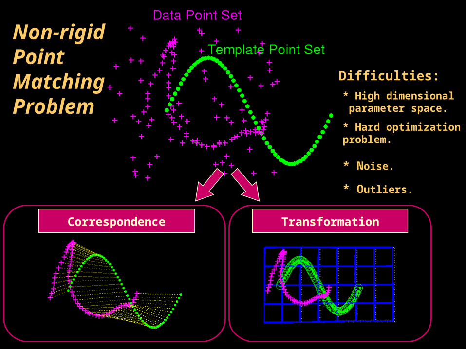
Non-rigid Point MatchingProblem
* Noise.
* Outliers.
* High dimensional parameter space.
* Hard optimization problem.
Difficulties:
Correspondence Transformation
},...,2,1,{ NixX i
},...,2,1,{ KavV a
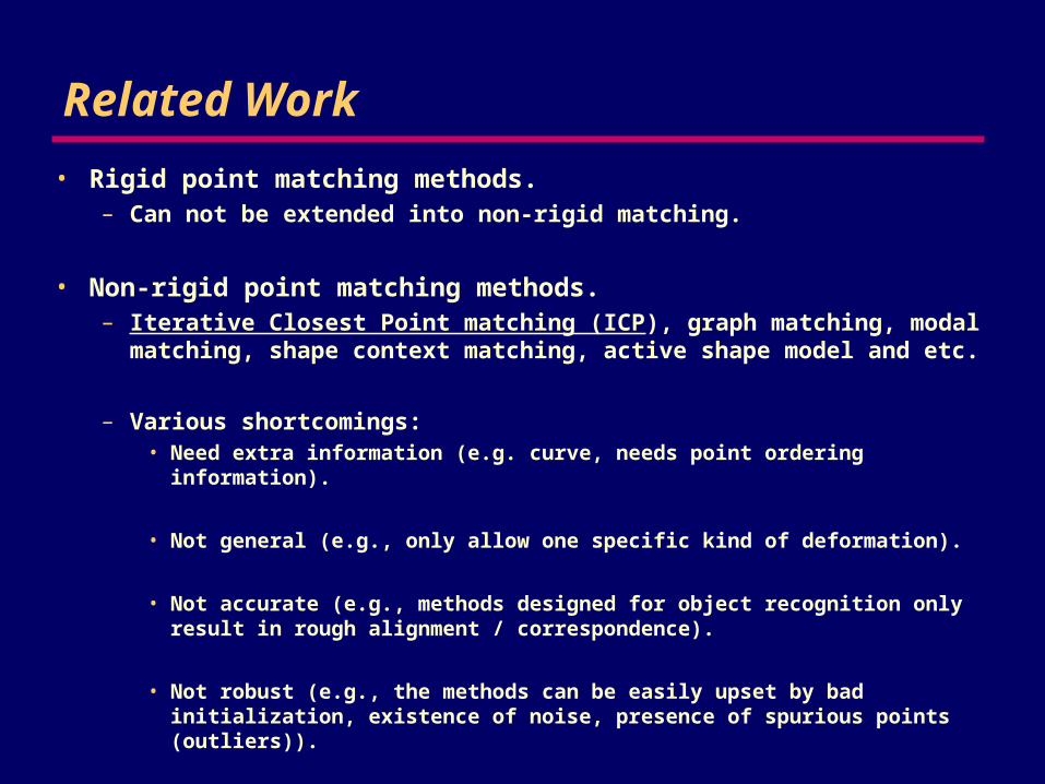
Related Work
• Rigid point matching methods.– Can not be extended into non-rigid matching.
• Non-rigid point matching methods.– Iterative Closest Point matching (ICP), graph matching, modal
matching, shape context matching, active shape model and etc.
– Various shortcomings:• Need extra information (e.g. curve, needs point ordering information).
• Not general (e.g., only allow one specific kind of deformation).
• Not accurate (e.g., methods designed for object recognition only result in rough alignment / correspondence).
• Not robust (e.g., the methods can be easily upset by bad initialization, existence of noise, presence of spurious points (outliers)).
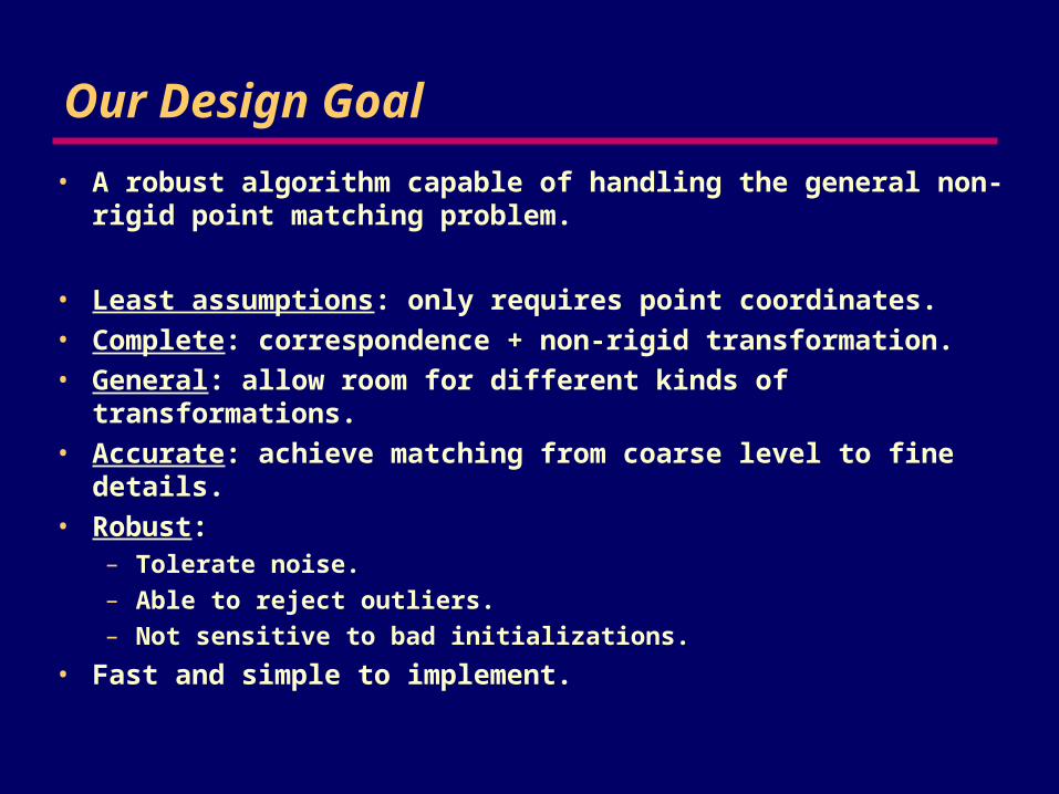
Our Design Goal
• A robust algorithm capable of handling the general non-rigid point matching problem.
• Least assumptions: only requires point coordinates.• Complete: correspondence + non-rigid transformation.• General: allow room for different kinds of transformations.• Accurate: achieve matching from coarse level to fine details.• Robust:
– Tolerate noise.
– Able to reject outliers.
– Not sensitive to bad initializations.
• Fast and simple to implement.
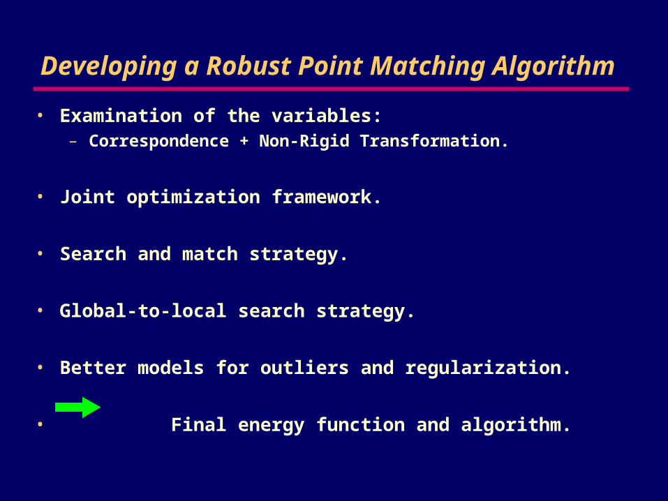
Developing a Robust Point Matching Algorithm
• Examination of the variables: – Correspondence + Non-Rigid Transformation.
• Joint optimization framework.
• Search and match strategy.
• Global-to-local search strategy.
• Better models for outliers and regularization.
• Final energy function and algorithm.
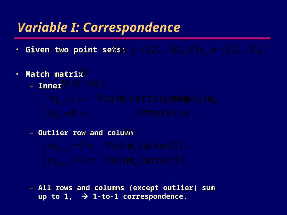
Variable I: Correspondence
• Given two point sets:
• Match matrix– Inner
– All rows and columns (except outlier) sum up to 1, 1-to-1 correspondence.
},...,2,1,{},,...,2,1,{ KavVNixX ai
M:)( NKM
Otherwise.0
.vpointtoscorrespondxPoint1 ai
ai
ai
m
m
– Outlier row and column :M
outlier.anisvPoint1
outlier.anisxPoint1
a1,
i,1
Na
iK
m
m
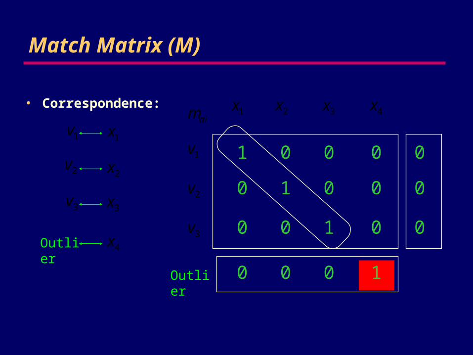
Match Matrix (M)
• Correspondence:
Outlier
Outlier
1
1000
00100
00010
00001v
2v
3v
1x
2x
3x
4x
1v
2v
3v
1x 2x 3x 4xaim
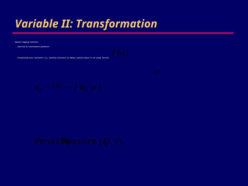
Variable II: Transformation• Spatial mapping function:
– Specified by transformation parameters:
– Incorporating prior constraints (e.g. smoothing constraint) by adding a penalty measure to the energy function.
).(f
.
).,()( a
fa vfv
.||||:MeasurePenalty 2Lf

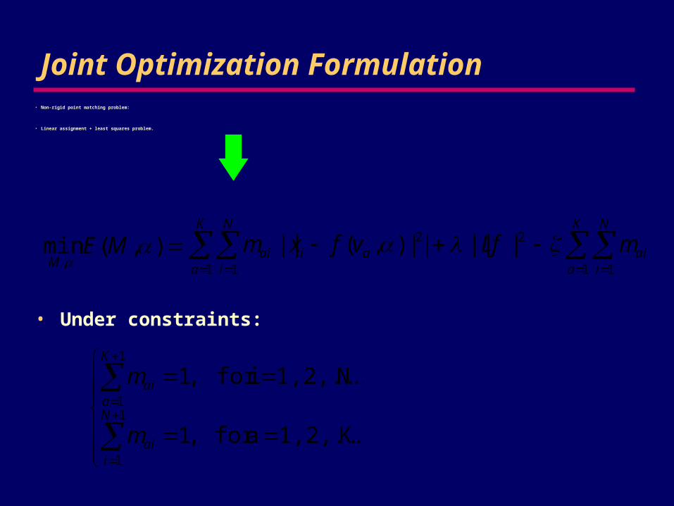
Joint Optimization Formulation• Non-rigid point matching problem:
• Linear assignment + least squares problem.
• Under constraints:
),(min,
MEM
K
a
N
iaiai vfxm
1 1
2||),(|| 2|||| Lf
K
a
N
iaim
1 1
K.1,2,...,afor ,1
N.1,2,...,ifor ,1
1
1
1
1N
iai
K
aai
m
m
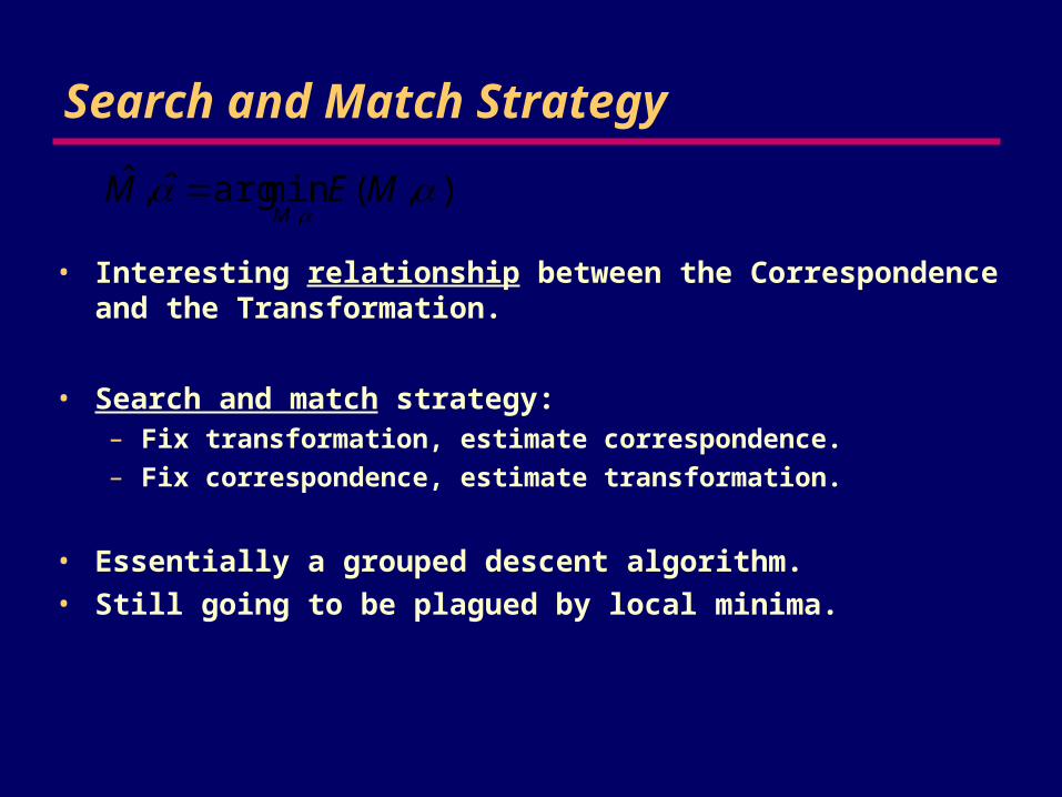
Search and Match Strategy
• Interesting relationship between the Correspondence and the Transformation.
• Search and match strategy:– Fix transformation, estimate correspondence.
– Fix correspondence, estimate transformation.
• Essentially a grouped descent algorithm. • Still going to be plagued by local minima.
),(minargˆ,ˆ,
MEMM
How to Overcome the Local Minima?
• Fuzzy correspondence.– A more flexible correspondence model.
• Deterministic annealing (DA).– Control the “fuzziness” of the correspondence.
• Accomplish matching:– global-to-local.
– coarse-to-fine.
Fuzzy Correspondence
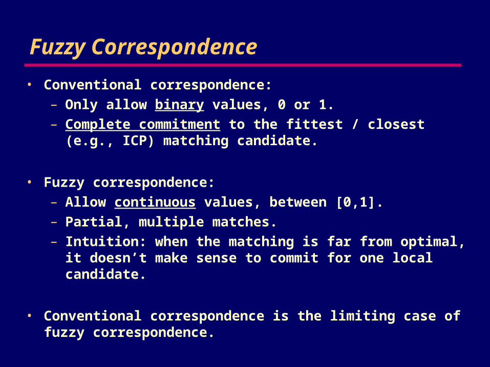
• Conventional correspondence:– Only allow binary values, 0 or 1.– Complete commitment to the fittest / closest (e.g., ICP)
matching candidate.
• Fuzzy correspondence:– Allow continuous values, between [0,1].– Partial, multiple matches.– Intuition: when the matching is far from optimal, it doesn’t
make sense to commit for one local candidate.
• Conventional correspondence is the limiting case of fuzzy correspondence.
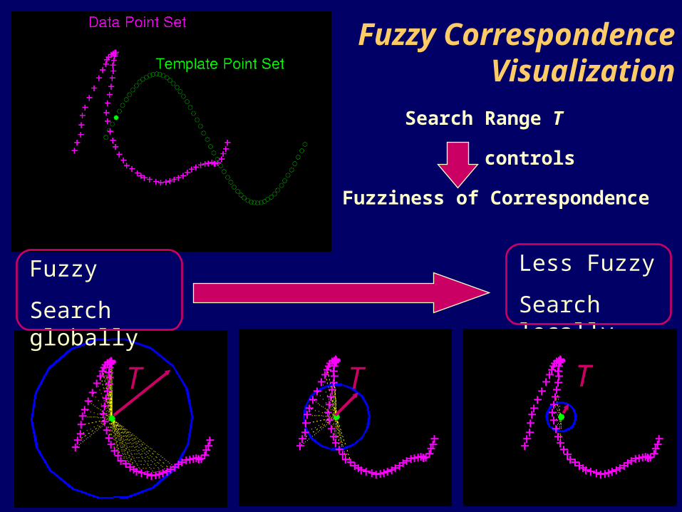
Fuzzy CorrespondenceVisualization
Fuzzy
Search globally
Less Fuzzy
Search locally
T
Search Range T
Fuzziness of Correspondence
controls
T T

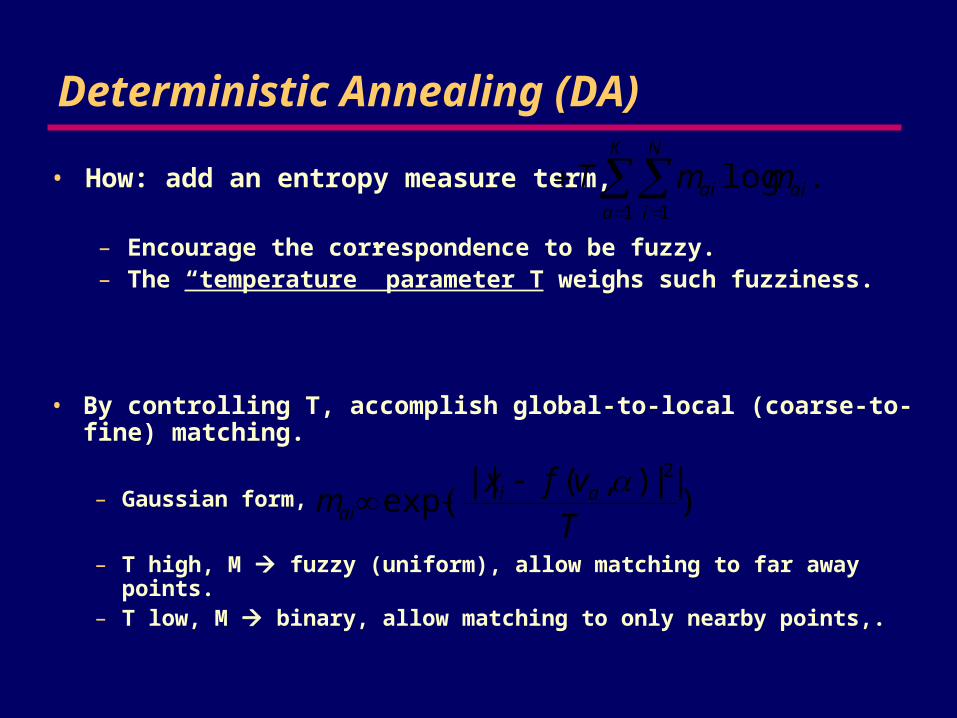
Deterministic Annealing (DA)
• How: add an entropy measure term, .log1 1
K
a
N
iaiai mmT
• By controlling T, accomplish global-to-local (coarse-to-fine) matching.
– Gaussian form,
– T high, M fuzzy (uniform), allow matching to far away points. – T low, M binary, allow matching to only nearby points,.
).||),(||
exp(2
T
vfxm ai
ai
– Encourage the correspondence to be fuzzy.– The “temperature” parameter T weighs such fuzziness.
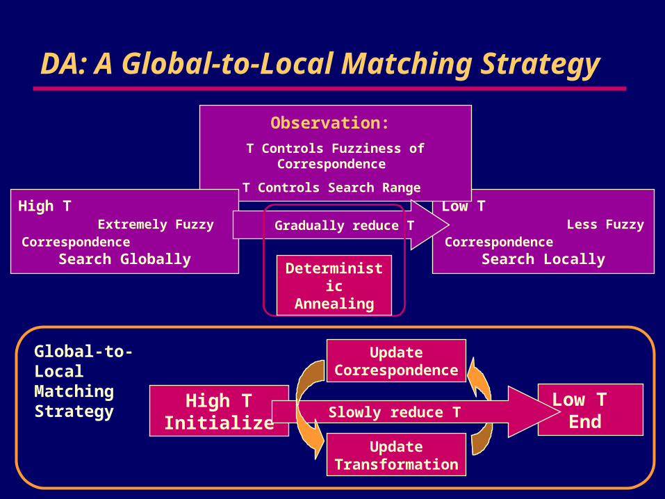
Low T Less Fuzzy Correspondence
Search Locally
Observation:
T Controls Fuzziness of Correspondence
T Controls Search Range
High T Extremely Fuzzy Correspondence
Search GloballyGradually reduce T
Deterministic Annealing
DA: A Global-to-Local Matching Strategy
Global-to-Local Matching Strategy High T
InitializeLow T
End
Update Correspondence
Slowly reduce T
Update Transformation
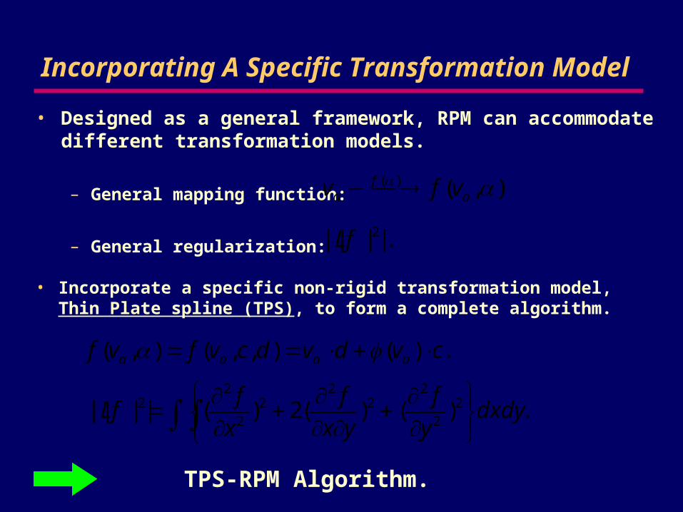
Incorporating A Specific Transformation Model
• Designed as a general framework, RPM can accommodate different transformation models.
– General mapping function:
– General regularization:
• TPS-RPM Algorithm.
).,()( a
fa vfv
.|||| 2Lf
• Incorporate a specific non-rigid transformation model, Thin Plate spline (TPS), to form a complete algorithm.
.)(),,(),( cvdvdcvfvf aaaa
.)()(2)(|||| 22
22
22
2
22
dxdyy
f
yx
f
x
fLf
Examples of RPM
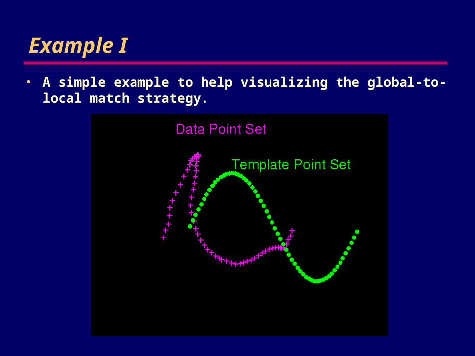
Example I
• A simple example to help visualizing the global-to-local match strategy.
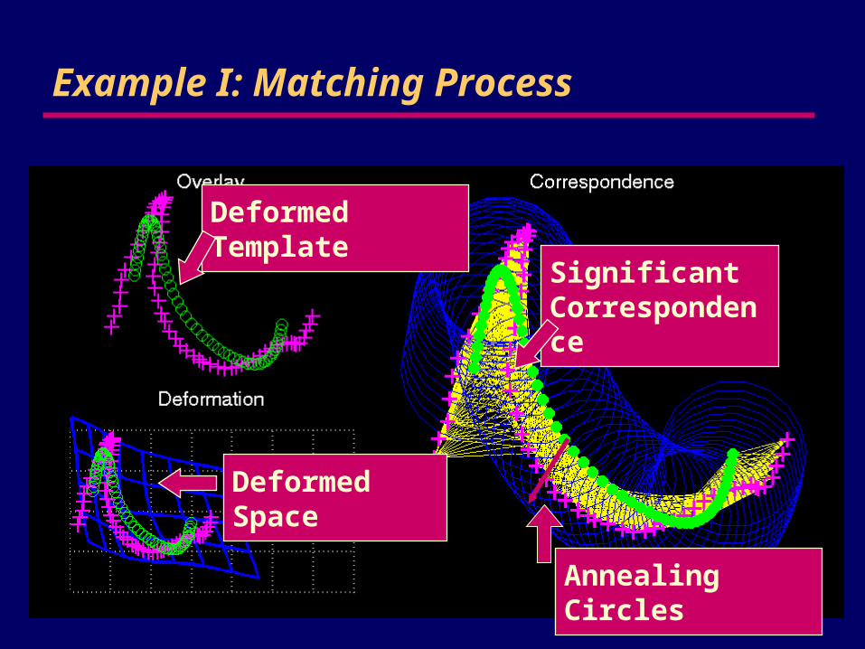
Deformed Template
Deformed Space
Significant Correspondence
Example I: Matching Process
Annealing Circles
T
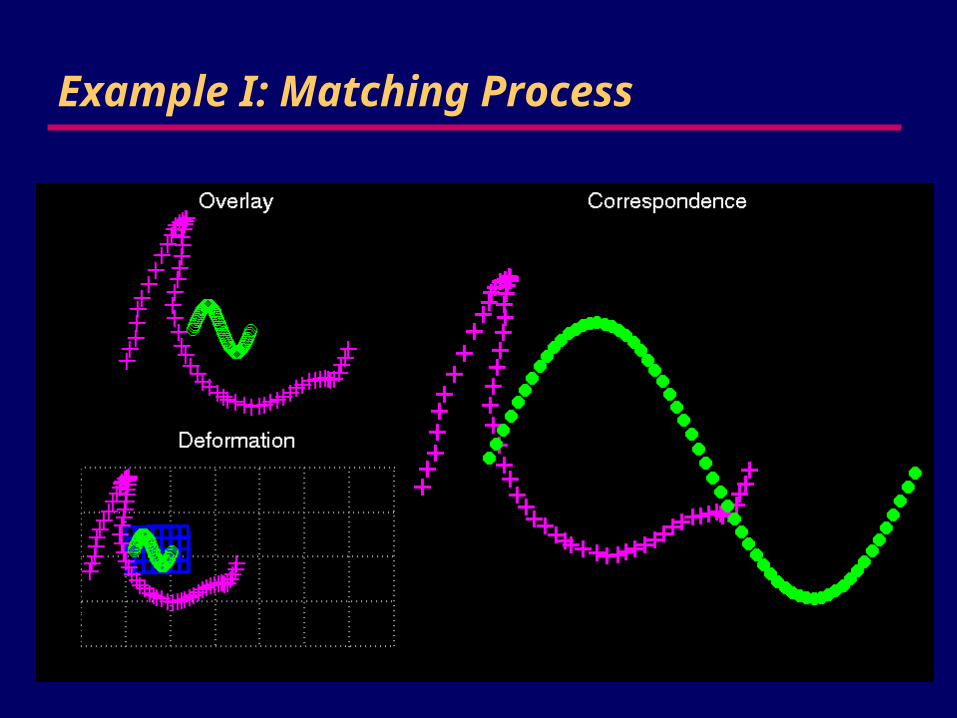
Example I: Matching Process
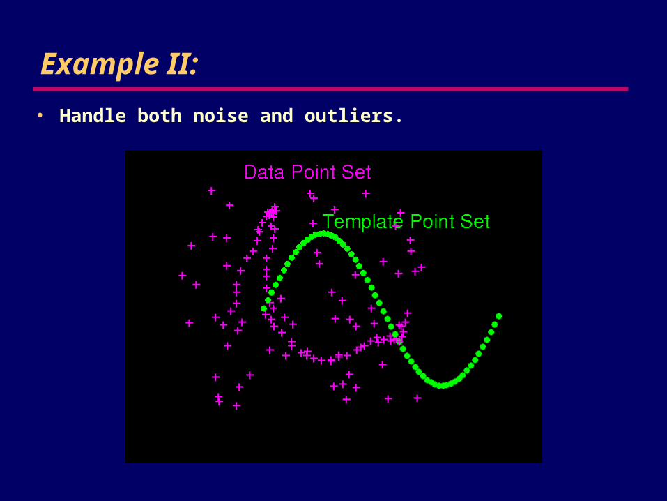
Example II:
• Handle both noise and outliers.
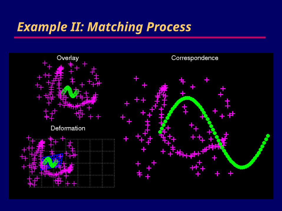
Example II: Matching Process
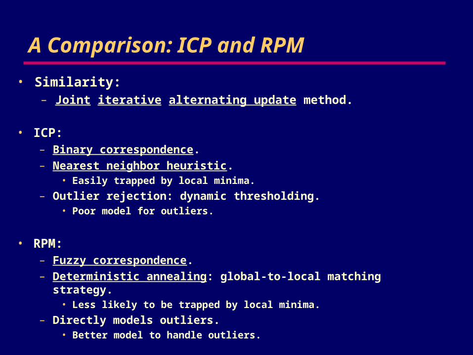
A Comparison: ICP and RPM
• Similarity:– Joint iterative alternating update method.
• ICP: – Binary correspondence.
– Nearest neighbor heuristic.• Easily trapped by local minima.
– Outlier rejection: dynamic thresholding.• Poor model for outliers.
• RPM: – Fuzzy correspondence.
– Deterministic annealing: global-to-local matching strategy.• Less likely to be trapped by local minima.
– Directly models outliers.• Better model to handle outliers.

Applications
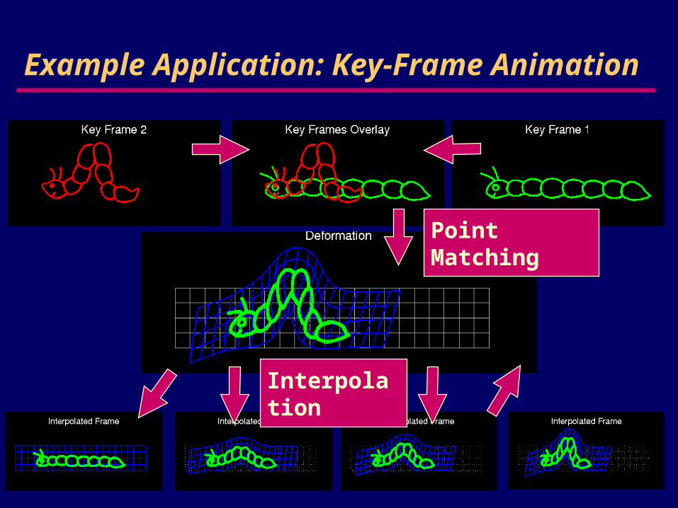
Point Matching
Interpolation
Example Application: Key-Frame Animation

Example Application: Key-Frame Animation
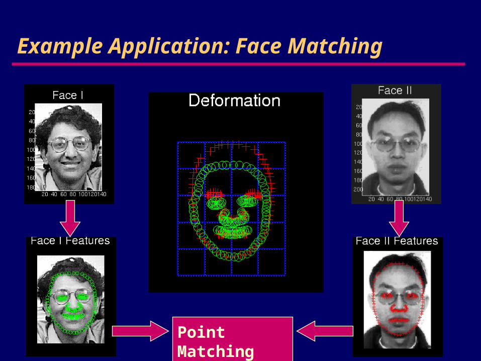
Point Matching
Example Application: Face Matching
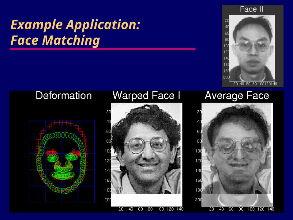
Example Application: Face Matching
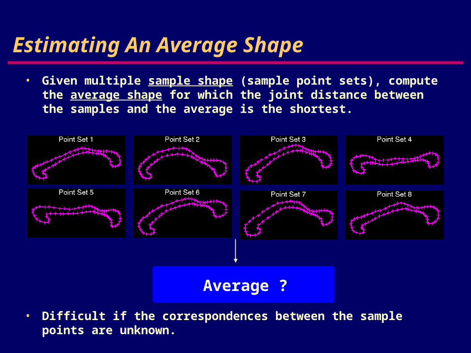
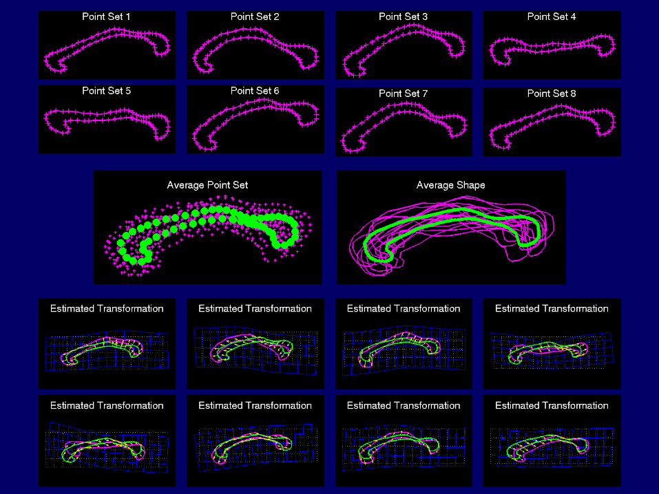
Estimating An Average Shape
• Given multiple sample shape (sample point sets), compute the average shape for which the joint distance between the samples and the average is the shortest.
Average ?
• Difficult if the correspondences between the sample points are unknown.

Application: Brain Anatomical Feature Registration (MRI Image)
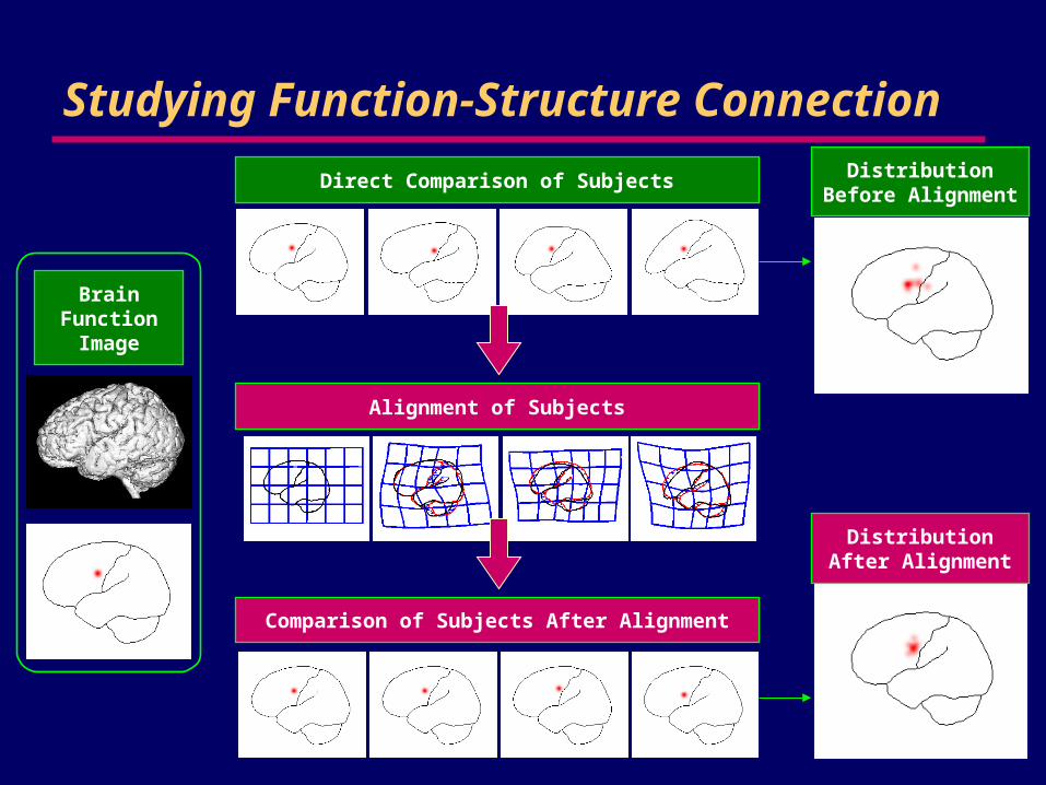
Studying Function-Structure Connection
Brain Function
Image
Alignment of Subjects
Comparison of Subjects After Alignment
Direct Comparison of Subjects Distribution Before Alignment
Distribution After Alignment
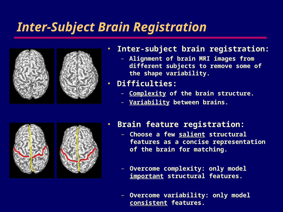
Inter-Subject Brain Registration
• Inter-subject brain registration: – Alignment of brain MRI images from different
subjects to remove some of the shape variability.
• Difficulties:– Complexity of the brain structure.– Variability between brains.
• Brain feature registration: – Choose a few salient structural features as a
concise representation of the brain for matching.
– Overcome complexity: only model important structural features.
– Overcome variability: only model consistent features.
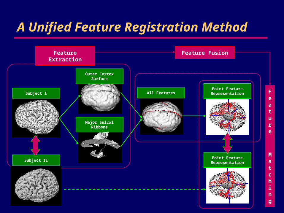
A Unified Feature Registration Method
Outer Cortex Surface
Major Sulcal Ribbons
All FeaturesPoint Feature
Representation
Point Feature Representation
Feature Extraction Feature Fusion
Feature
Matching
Subject I
Subject II
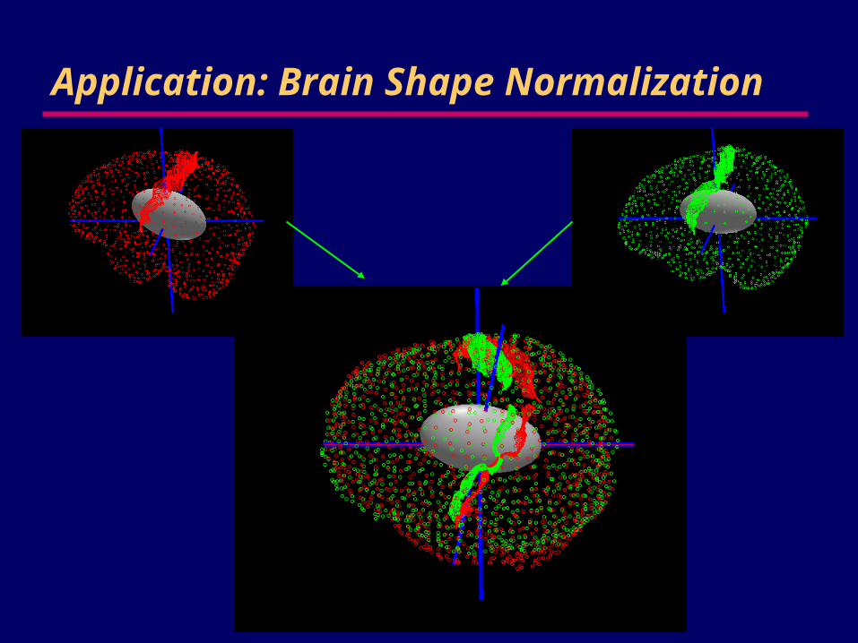
Application: Brain Shape Normalization
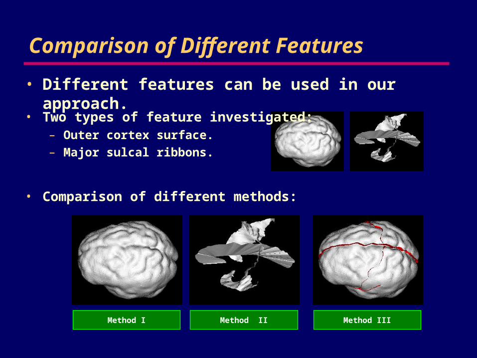
Comparison of Different Features
• Different features can be used in our approach.
• Two types of feature investigated:– Outer cortex surface.
– Major sulcal ribbons.
• Comparison of different methods:
Method I Method II Method III
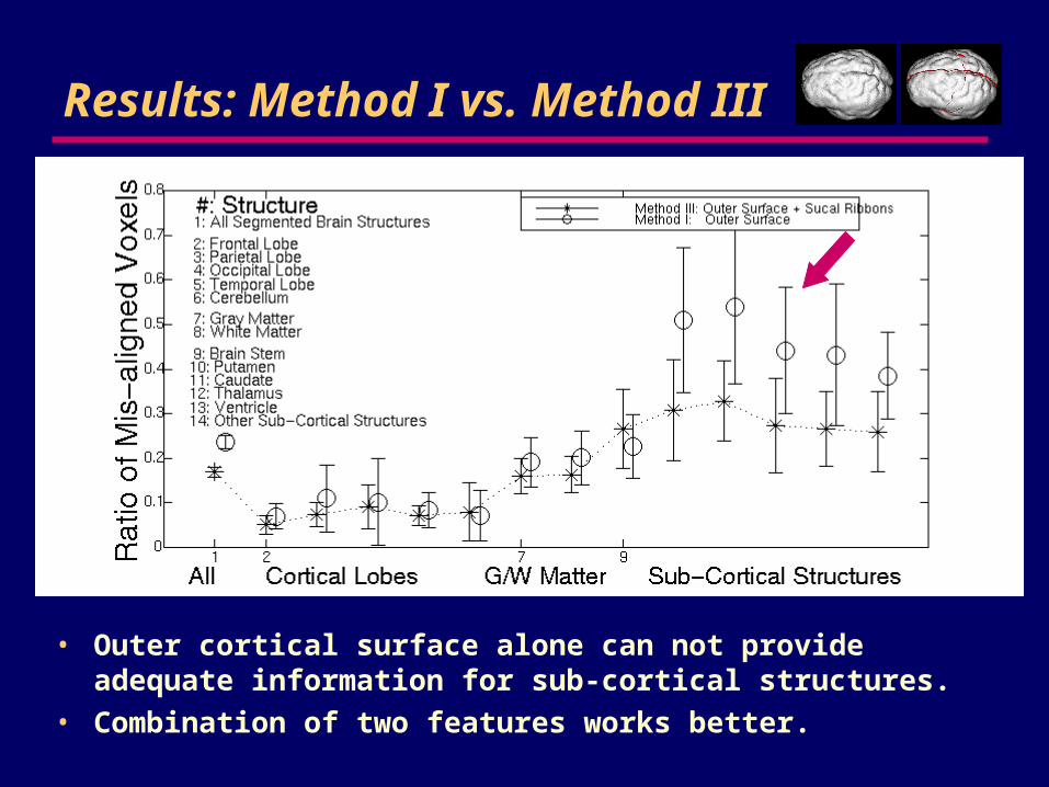
Results: Method I vs. Method III
• Outer cortical surface alone can not provide adequate information for sub-cortical structures.
• Combination of two features works better.
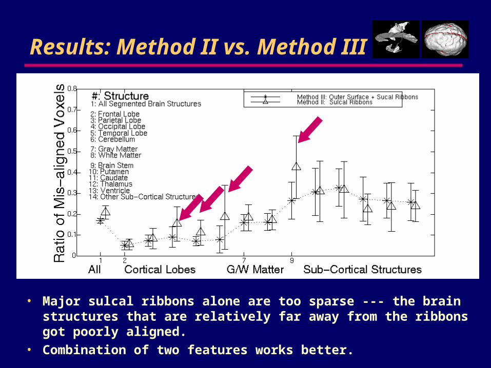
Results: Method II vs. Method III
• Major sulcal ribbons alone are too sparse --- the brain structures that are relatively far away from the ribbons got poorly aligned.
• Combination of two features works better.
Conclusion
• Unified brain feature registration approach:– Combination of different features improves registration.
– Benefits: general/unified, symmetric, efficient.
• Robust point matching algorithm:– Capable of estimating non-rigid transformations and
correspondences.
– Robust (noise/outliers/initializations).
• Non-rigid point matching can be a general tool for many different problems.
Future Work
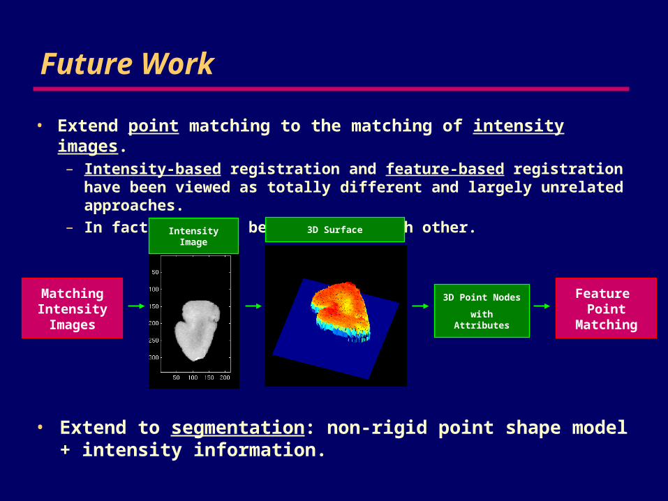
• Extend point matching to the matching of intensity images.– Intensity-based registration and feature-based registration have
been viewed as totally different and largely unrelated approaches.
– In fact, they can be related to each other.
Intensity Image
Matching Intensity Images
3D Surface
Feature Point Matching
3D Point Nodes
with Attributes
• Extend to segmentation: non-rigid point shape model + intensity information.
Future Work
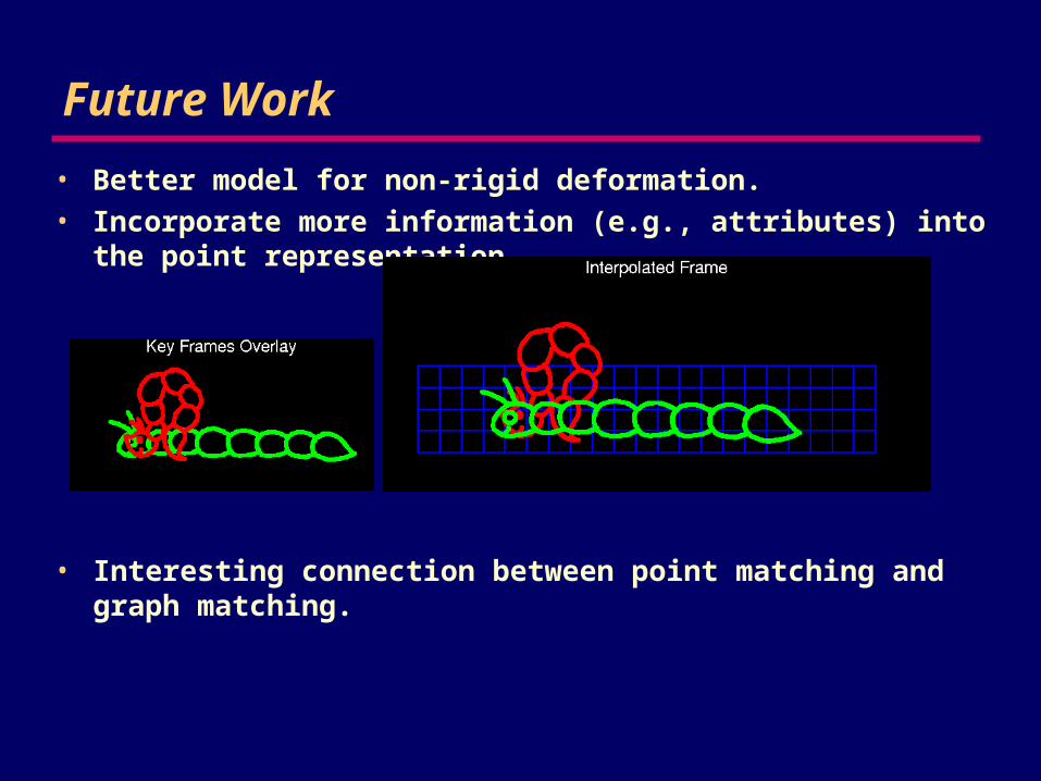
• Better model for non-rigid deformation.• Incorporate more information (e.g., attributes) into the point
representation.
• Interesting connection between point matching and graph matching.
Acknowledgements
• Thesis advisor and committee members:– Anand Rangarajan, James Duncan, Hemant Tagare and Peter
Schultheiss.
• IPAG members:– Lawrence Staib, Xiaolan Zeng, Xenios Papademetris, Oskar Skrinjar,
Ravi Bansal, Yongmei Wang, Pengcheng Shi, James Rambo, Gang Liu, Ning Lin, Xiaoning Qian, Zhong Tao and Jing Yang.
• Colleagues in the brain registration project:– Robert Schultz, Lawrence Win and Joseph Walline.
• Financial support is provided by the grants from the Whitaker Foundation, NSF, NIH.
• Further information: http://noodle.med.yale.edu/~chui/.

RPM Detail
Joint Optimization Formulation• Non-rigid point matching problem:
• Linear assignment + least squares problem.
• Under constraints:
),(min,
MEM
K
a
N
iaiai vfxm
1 1
2||),(|| 2|||| Lf
K
a
N
iaim
1 1
K.1,2,...,afor ,1
N.1,2,...,ifor ,1
1
1
1
1N
iai
K
aai
m
m
Deterministic Annealing (DA)
• How: add an entropy measure term, .log1 1
K
a
N
iaiai mmT
• By controlling T, accomplish global-to-local (coarse-to-fine) matching.
– Gaussian form,
– T high, M fuzzy (uniform), allow matching to far away points. – T low, M binary, allow matching to only nearby points,.
).||),(||
exp(2
T
vfxm ai
ai
– Encourage the correspondence to be fuzzy.– The “temperature” parameter T weighs such fuzziness.

Two More Modifications
• Poor outlier model.
• Poor regularization model.
– Robustness term:
– In-direct model.– Parameter hard to estimate.
– Constant regularization term:
– Regularization can be too much or too little.
– Parameter hard to estimate.
2|||| Lf
K
a
N
iaim
1 1
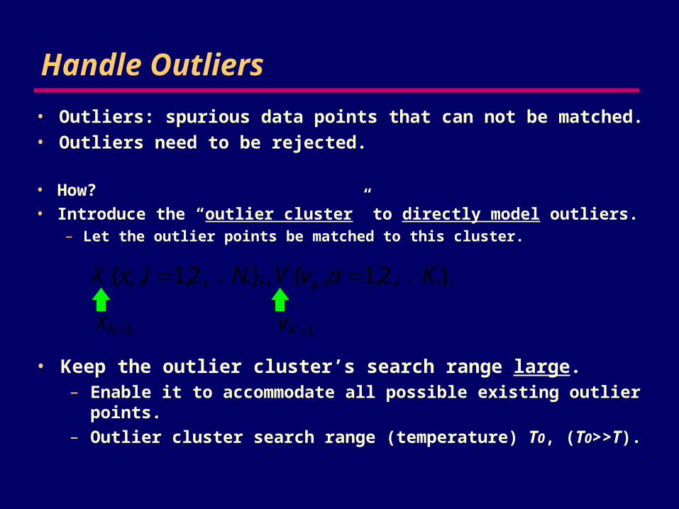
Handle Outliers
• Outliers: spurious data points that can not be matched.• Outliers need to be rejected.
• Keep the outlier cluster’s search range large.– Enable it to accommodate all possible existing outlier points.
– Outlier cluster search range (temperature) T0, (T0>>T).
• How?• Introduce the “outlier cluster” to directly model outliers.
– Let the outlier points be matched to this cluster.
},...,2,1,{},,...,2,1,{ KavVNixX ai
1Nx 1Kv
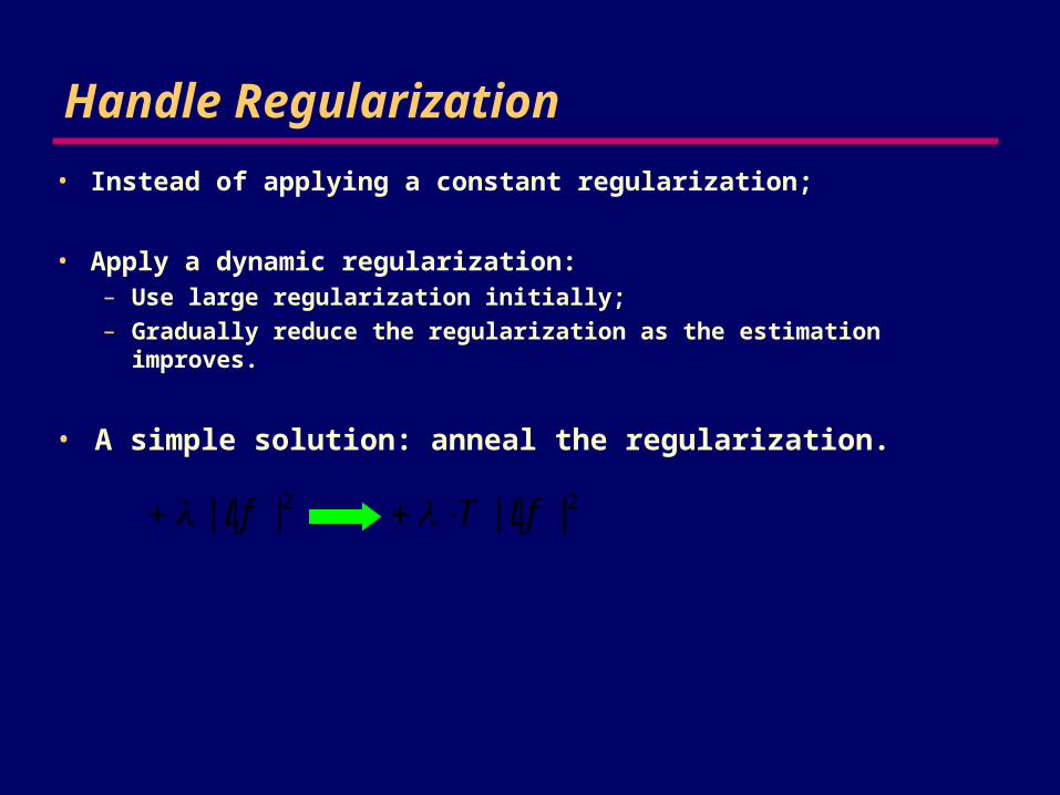
Handle Regularization
• Instead of applying a constant regularization;
• Apply a dynamic regularization:– Use large regularization initially;
– Gradually reduce the regularization as the estimation improves.
• A simple solution: anneal the regularization.
2|||| Lf 2|||| LfT
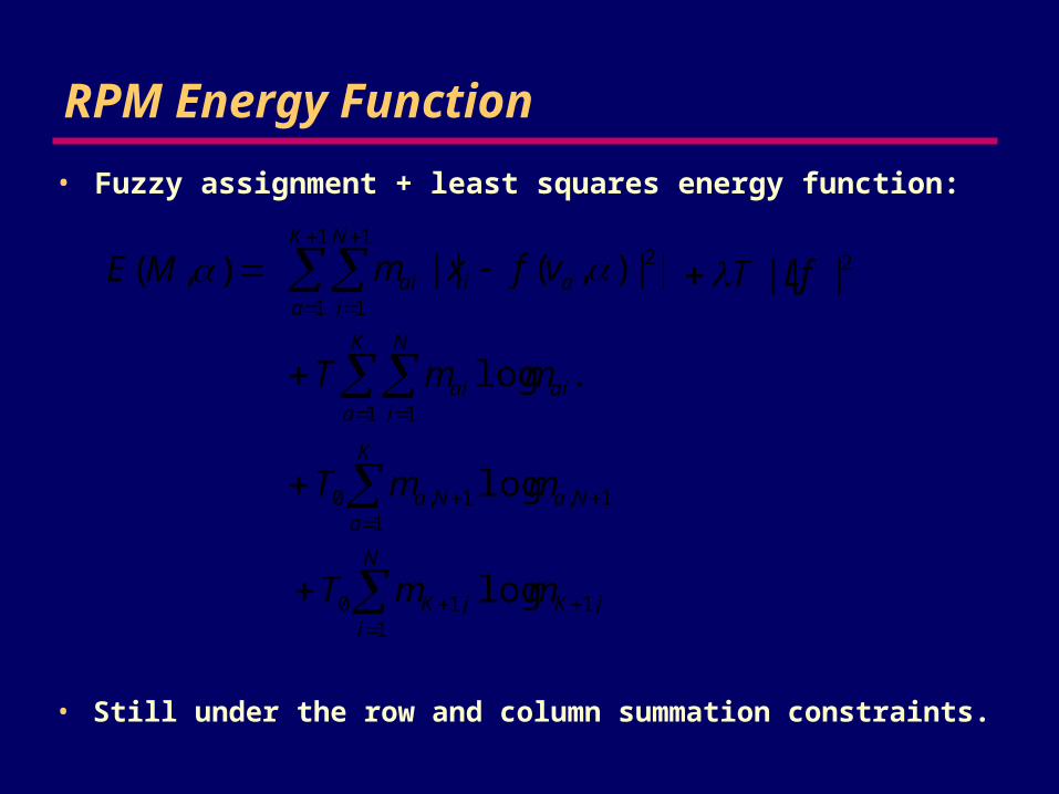
RPM Energy Function
• Fuzzy assignment + least squares energy function:
• Still under the row and column summation constraints.
),( ME
1
1
1
1
2||),(||K
a
N
iaiai vfxm 2|||| LfT
.log1 1
K
a
N
iaiai mmT
K
aNaNa mmT
11,1,0 log
N
iiKiK mmT
1,1,10 log

• Initialize parameters
• Initialize parameters (or ).
• Deterministic annealing.
• Lower until is reached.
Alternating update:
Given , update .
Given , update .
RPM Algorithm
T Tf inal
• Basically a dual alternating update process embedded within a deterministic annealing scheme.
MM
M
.,0 TT
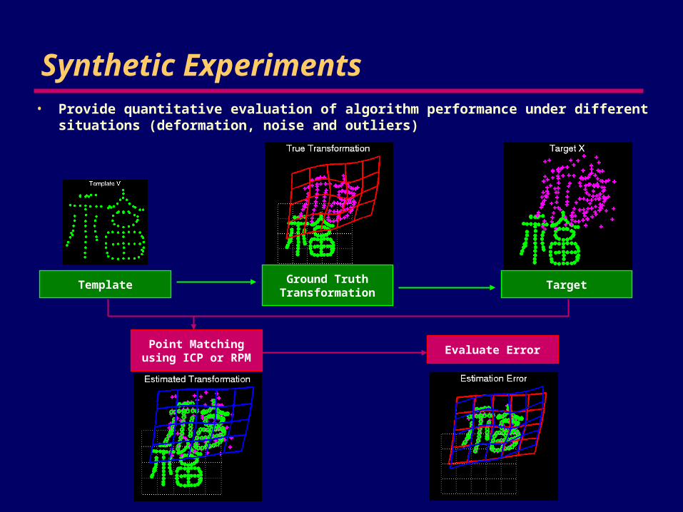
Synthetic Experiments• Provide quantitative evaluation of algorithm performance under different situations
(deformation, noise and outliers)
Template Ground Truth Transformation
Target
Evaluate ErrorPoint Matching using ICP or RPM
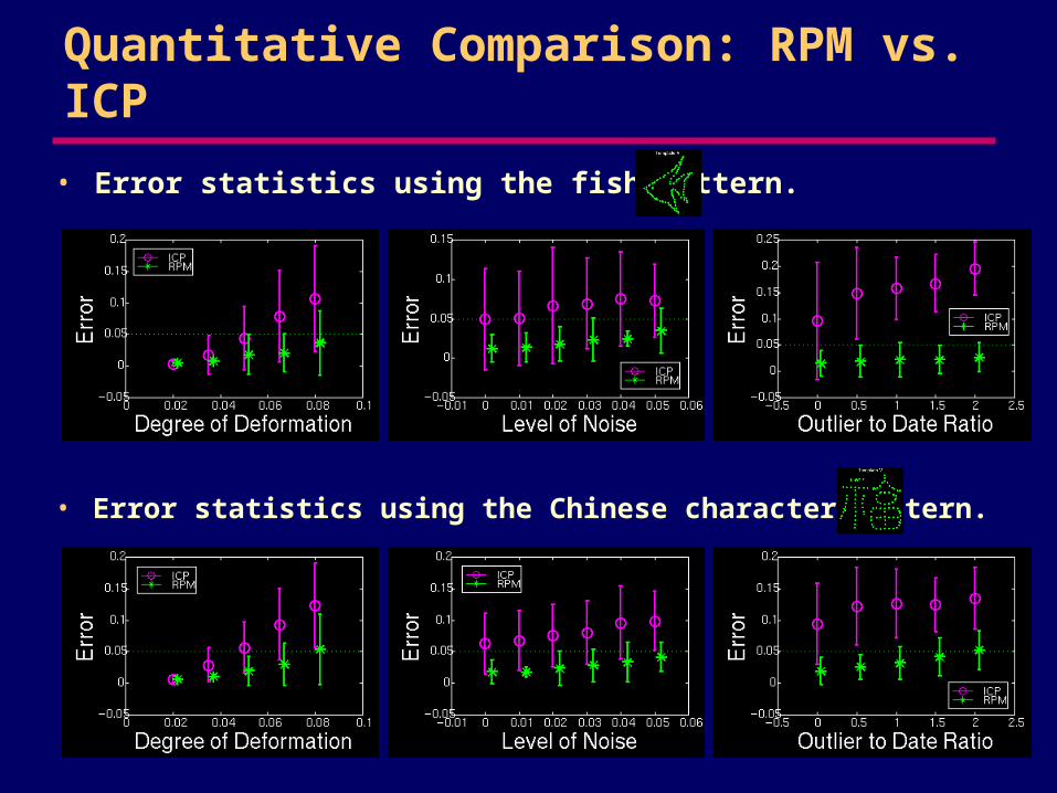
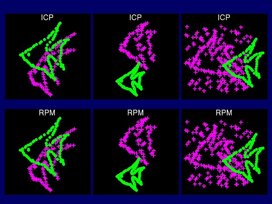
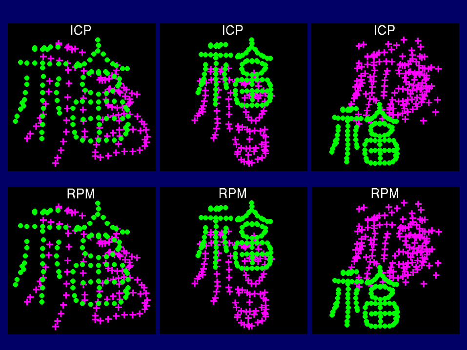
Quantitative Comparison: RPM vs. ICP
• Error statistics using the fish pattern.
• Error statistics using the Chinese character pattern.

“Super” Clustering-Matching Algorithm (SCM)
• Diagram:
MatchingMatchable
ClustersOutlier Cluster
Clusters Center Set V
Clustering
Matchable Clusters
Outlier Cluster
Clusters Center Set U
Clustering
Point Set X Point Set Y
Average Point Set Z
Matching and
Estimating
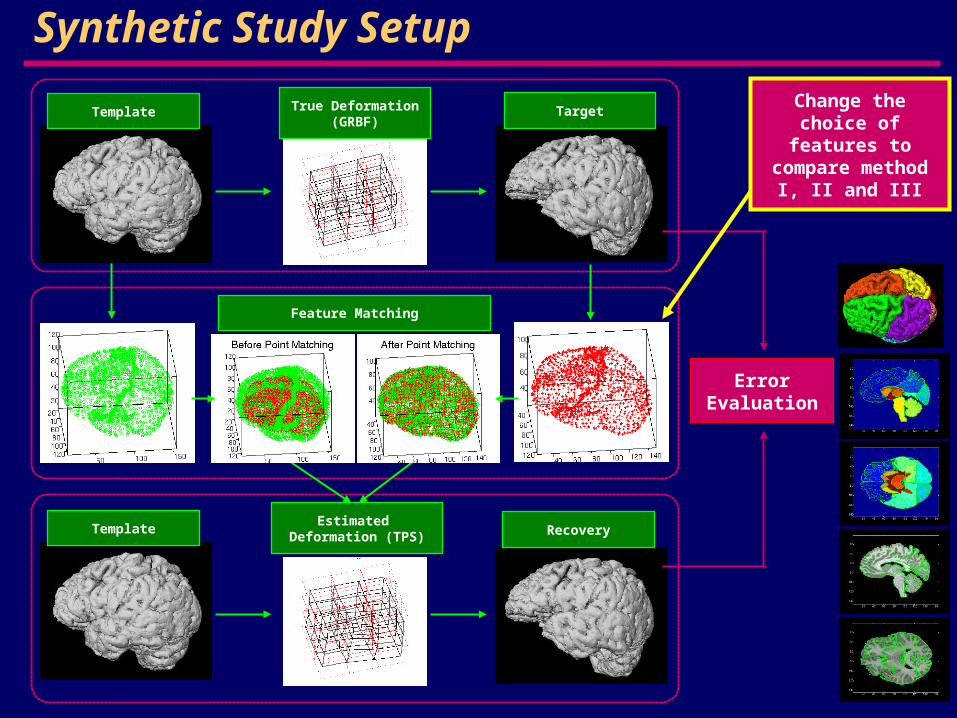
Synthetic Study Setup
Template True Deformation (GRBF)
Target
Template RecoveryEstimated Deformation
(TPS)
Error Evaluation
Feature Matching
Change the choice of features to
compare method I, II and III

Mixture Model
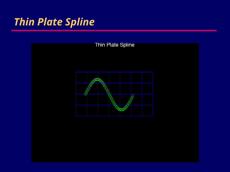
Thin Plate Spline
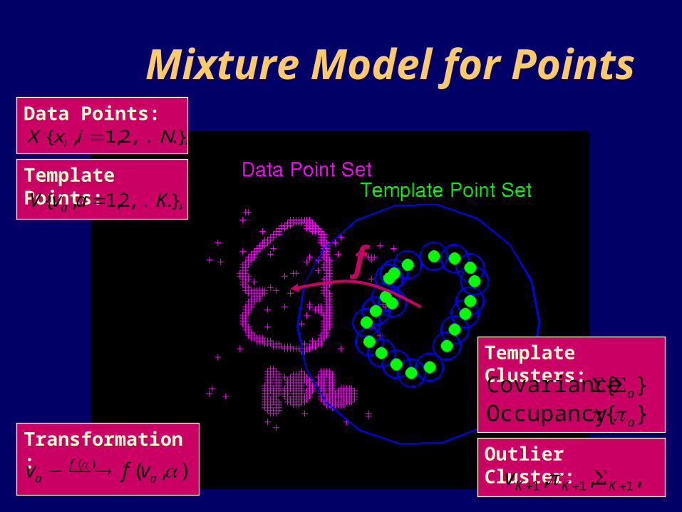
Mixture Model for Points
f
Template Points:
Data Points:},...,2,1,{ NixX i
},...,2,1,{ KavV a
Transformation:
).,()( a
fa vfv
Template Clusters:
}.{Covariance a}.{Occupancy a
Outlier Cluster:,.,, 111 KKKv
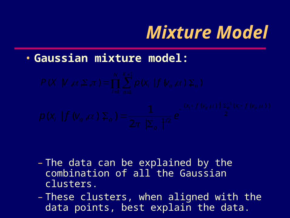
Mixture Model• Gaussian mixture model:
– The data can be explained by the combination of all the Gaussian clusters.
– These clusters, when aligned with the data points, best explain the data.
).),,(|(),,,|(1
11aa
K
ai
N
i
vfxpVXP
2
)),(()),((
2/1
1
||2
1)),,(|(
aiaT
ai vfxvfx
aaai evfxp
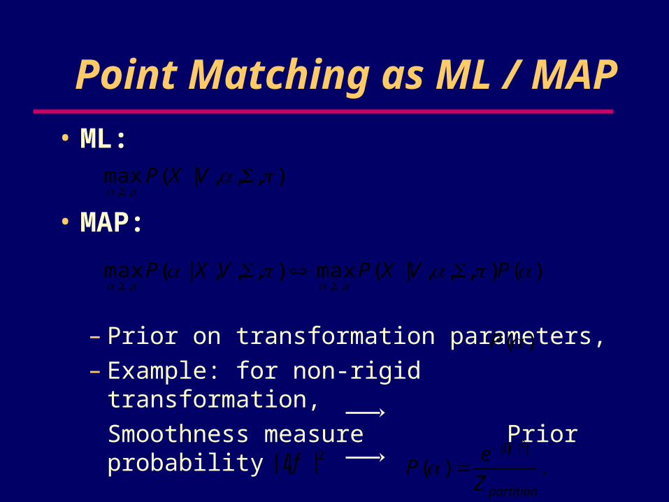
Point Matching as ML / MAP
• ML:
• MAP:
– Prior on transformation parameters,– Example: for non-rigid transformation,
Smoothness measure Prior probability
),,,|(max,,
VXP
)(),,,|(max),,,|(max,,,,
PVXPVXP
).(P
2|||| Lf .)(2||||
partition
Lf
Z
eP
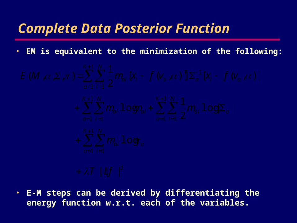
Complete Data Posterior Function
• EM is equivalent to the minimization of the following:
),,,( ME
1
1 1
1 )],([)],([2
1K
a
N
iaia
Taiai vfxvfxm
2|||| LfT
1
1 1
logK
a
N
iaiai mm
1
1 1
||log2
1K
a
N
iaaim
1
1 1
logK
a
N
iaaim
• E-M steps can be derived by differentiating the energy function w.r.t. each of the variables.
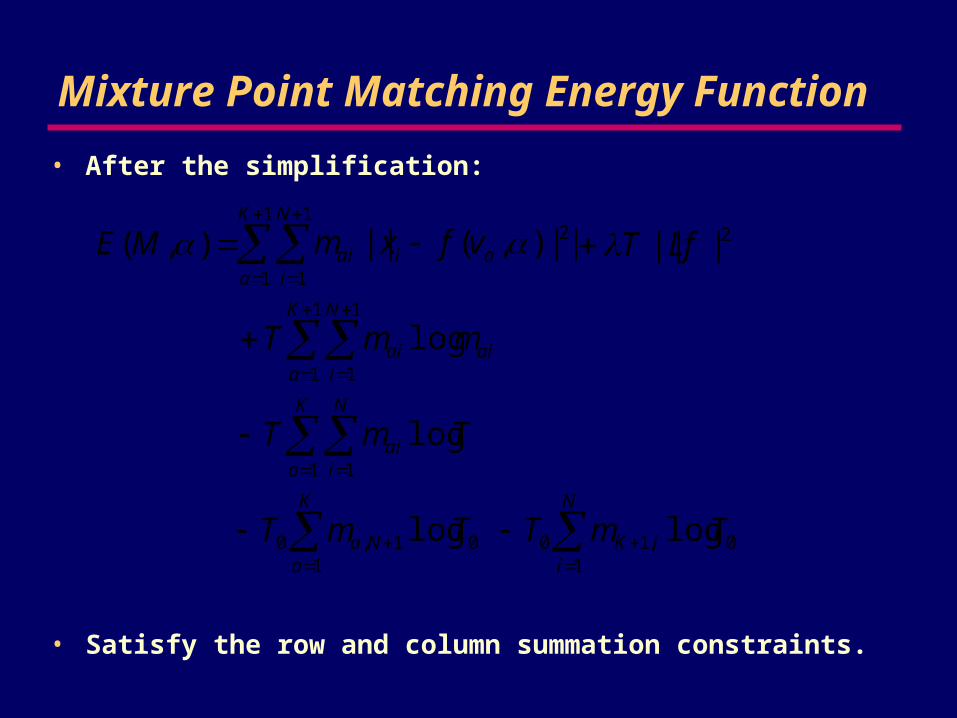
Mixture Point Matching Energy Function
• After the simplification:
• Satisfy the row and column summation constraints.
),( ME
1
1
1
1
2||),(||K
a
N
iaiai vfxm 2|||| LfT
1
1
1
1
logK
a
N
iaiai mmT
K
aNa TmT
101,0 log
N
iiK TmT
10,10 log
K
a
N
iai TmT
1 1
log
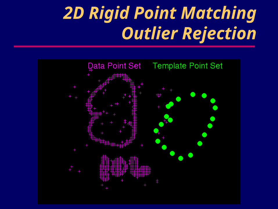
2D Rigid Point MatchingOutlier Rejection
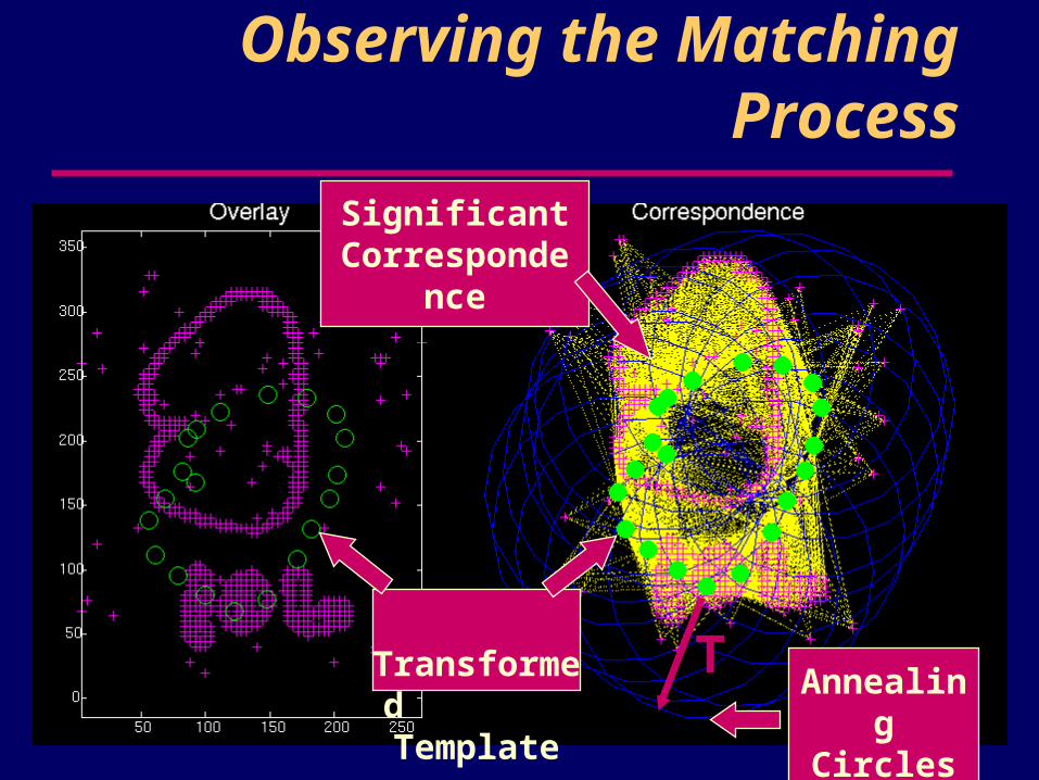
Observing the Matching Process
Transformed
TemplateAnnealing
Circles
T
Significant Correspondence
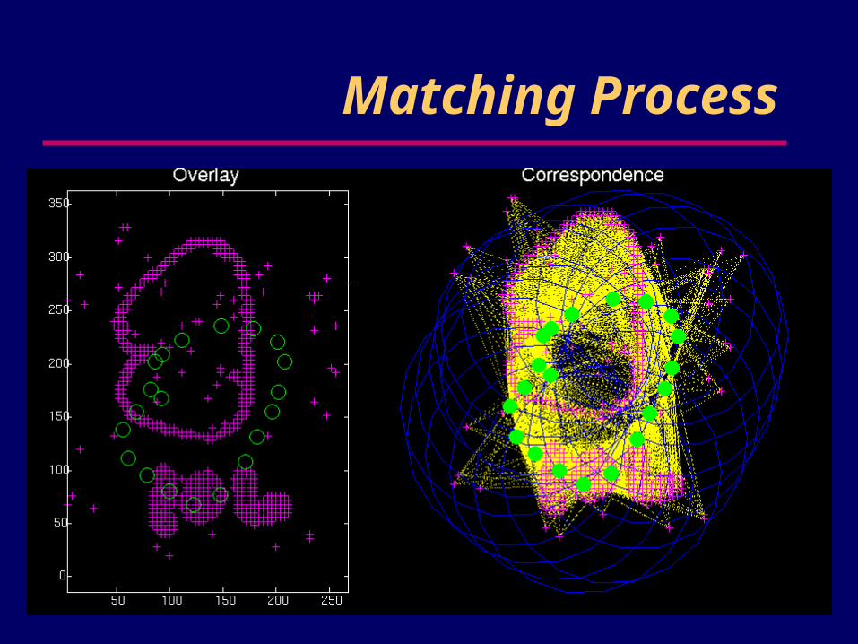
Matching Process