Reduced-Order Modeling of Hypersonic Unsteady … · Reduced-Order Modeling of Hypersonic Unsteady Aerodynamics Due to ... This is not intended to be representative of any speci c

Reduced-Order Modeling of Hypersonic Unsteady Aerodynamics Due to

Multi-Modal Oscillations

Torstens Skujins �

Carlos E. S. Cesnik y

University of Michigan, Ann Arbor, Michigan 48109

The development of hypersonic vehicle control algorithms requires the ac-curate prediction of vehicle aerodynamic loads. This paper focuses on �ndingtime-accurate unsteady loads due to the oscillation of multiple vehicle elasticmodes. The reduced-order modeling methodology consists of using convolu-tion of modal step responses along with a correction factor to take di�erentoscillation amplitudes, ight conditions, and nonlinear aerodynamic e�ects dueto multi-modal oscillations into account. Thus, the model is valid over a rangeof conditions rather than one speci�c set of conditions upon which it is con-structed. When compared with CFD simulations, the errors are shown to berelatively small in most cases over a range of Mach numbers, modal frequen-cies, and modal oscillation amplitudes. Also, an error estimation methodologyis developed to give a general sense beforehand as to the errors expected tobe incurred through the use of the model.

I. Introduction

Among the many challenges faced in the design of hypersonic vehicles is the development of accuratecontrol algorithms. The aerodynamic forces in the hypersonic regime are quite large, so any mispredictionof these loads will potentially result in inaccurate control algorithms, which in turn could result in loss ofcontrol of the vehicle. Even though hypersonic vehicles are inherently sti� structures, they still do experience exible deformations while in ight. Thus, to accurately model the aerodynamic loads on the vehicle, it isimportant to create the tools to accurately model the unsteady aerodynamic e�ects caused both by thesestructural deformations as well as rigid body pitch/plunge motions.

Computational uid dynamics (CFD)-based reduced-order models provide an e�ective way to model theunsteady aerodynamic loads. Once constructed, the models run orders of magnitude faster than full CFDsolutions while preserving a high level of the accuracy seen by the computational simulations. However, amajor drawback of many reduced-order models is that they are only valid for ight conditions immediatelyaround those from which the model was constructed. E�orts have been made to make the ROMs validover a range of parameters. Glaz et al.1 use an unsteady surrogate-based approach to construct a modelfor unsteady rotorcraft dynamics over a range of pitch/plunge motions and Mach numbers. Silva2 uses aconvolution-type of methodology to construct a state-space ROM which is then used over a range of velocitiesin the transonic regime by modifying the time step of the numerical integration. Other e�orts for parameter-independent ROMs have focused on the analysis of ight test data. Lind et al.3 create velocity-independentkernels by using curve �ts of ight test data gathered at di�erent conditions. Baldelli et al.4 create a modelvalid over a range of dynamic pressures by combining linear and nonlinear operators for model construction.Prazenica et al.5 extrapolate kernels found at di�erent ight conditions to create one model valid overa range of conditions. Omran and Newman6 use Volterra series submodels in di�erent domains, such aspre-stall and post-stall, to construct an overall global piecewise Volterra series model.�Graduate Research Assistant, University of Michigan, Email: [email protected], Member AIAA.yProfessor, Department of Aerospace Engineering, University of Michigan, Email: [email protected], 1320 Beal Avenue,

3024 FXB, Ann Arbor, MI 48109-2140, Ph. (734) 764-3397, Fax: (734) 764-0578, AIAA Associate Fellow.

1 of 14

American Institute of Aeronautics and Astronautics

17th AIAA International Space Planes and Hypersonic Systems and Technologies Conference 11 - 14 April 2011, San Francisco, California

AIAA 2011-2341

Copyright © 2011 by Torstens Skujins and Carlos E.S. Cesnik. Published by the American Institute of Aeronautics and Astronautics, Inc., with permission.

Ref. 7 lays out the basic framework for a reduced-order model (ROM) technique for the hypersonic vehicleunsteady aerodynamics. The methodology is based on the convolution of modal step responses combinedwith a nonlinear correction factor to account for amplitudes of motion and ight conditions away from thosearound which the ROM was constructed. However, as detailed in the paper, the method was limited tocases with only a single mode of oscillation. This work extends this formulation to take into account multi-modal oscillations and provides an assessment of the e�ects of reduced frequency on the accuracy of themodel. In order to construct the nonlinear correction factor, a certain number of CFD sampling runs mustbe completed. This work also lays out a quantitative metric for determining an optimal number of samplingpoints to use and provides an estimate of the errors expected to be incurred through the use of the ROMmethodology.

II. ROM Methodology

A convolution-based ROM was chosen due to the ease of implementation into a CFD code. In general,the process involves convolving the modal step response with arbitrary modal motion to �nd the uncorrectedROM response. Then, the nonlinear correction factor is applied to give the �nal corrected ROM response.The overall unsteady aerodynamic ROM framework is shown in Fig. 1. The inputs are the structural modeshapes and modal amplitudes at each time step, from which the modal motion can be obtained. The outputsare the time-accurate coe�cients and/or generalized aerodynamic forces. See Ref. 7 for details on the CFDruns necessary for model construction.

Figure 1. Unsteady aerodynamic ROM schematic

A. Convolution

The response of a linear system to an arbitrary input can be found if the response of the system to a unitstep (H (t)) or unit impulse (h (t)) function is known. The response y(t) due to an arbitrary input f(t) isfound through the use of convolution:8;9

y (t) = f (0)H (t) +Z t

0

df

dt(�)H (t� �) d� (1)

Since the unit impulse is the derivative of the unit step, integration by parts yields

2 of 14


y (t) = f (t)H (0) +Z t

0

f (�)h (t� �) d� (2)

Equations 1 and 2 are the two forms of Duhamel’s integral.The reduced-order model presented here is based on the step convolution described above. Volterra series

is the nonlinear extension of convolution. However, for the cases tested here, the ROM using convolutionand the correction factor described subsequently showed improved agreement with direct CFD results whencompared with Volterra results. The uncorrected ROM solution is found by convolving the arbitrary modalmotion with CFD modal step input response results.

B. Correction Factor, Single Mode

The results in Ref. 7 showed that, as the input amplitude and ight conditions strayed from those used inthe step response, the accuracy of the lift, drag, and moment coe�cients signi�cantly decreased. Thus, anonlinear correction factor was introduced, de�ned as follows for the oscillation of a single mode:

fc =Y2Y1

d2d1

(3)

In Eq. 3, Y1 is the �nal, quasi-steady response (cl or other coe�cient) to a step input of amplitude d1, andY2 is the �nal response to an input of amplitude d2, which may also be at a di�erent ight condition. For alinear system, this ratio would always equal 1, as the outputs scale with the inputs.

Latin hypercube testing combined with kriging methodology was used to construct surfaces for fc pertain-ing to each of the coe�cients throughout the parameter space of interest. Results showed that multiplyingthe convolved response with this correction factor greatly improved the accuracy of the reduced-order model.

C. Kriging

Kriging is a methodology which creates surface �ts of functions using sampling data points obtained throughcomputational experiments. Unlike actual experiments, which inherently contain random error, computa-tional simulations will give the same answer for the same simulation when repeated. Thus, a kriging surfacewill pass through all test points, whereas a least squares �t surface will not in general directly pass througheach point. This is accomplished through the use of a regression model coupled with a random function.Refs. 10 and 11 provide detailed explanations of the kriging methodology and model construction.

D. Correction Factor, Multiple Modes

The extension of the correction factor to multiple modes is investigated at �rst using two di�erent methods.Consider a sample airfoil undergoing oscillations in each of the �rst m modes. The �rst method is to simplyuse superposition of individual modal responses to �nd the total response. Using this method, the responseof each mode is calculated as detailed above. Then, each response is added together to �nd the �nal response.

The second method is to create a correction factor that can be easily extended to multiple modes. This canbe accomplished by de�ning the multi-modal correction factor fcm as follows, here presented for simplicityas a three-mode excitation:

fcm =Y123 � �

Y1 + Y2 + Y3 � �(4)

In Eq. 4, Y123 is the �nal quasi-steady response after steps of certain amplitudes have been simultaneouslyapplied to each of the �rst three modes; the denominator is the superposition of uncorrected individualmodal responses Y1, Y2, and Y3; and � is an o�set introduced to prevent numerical issues. A kriging surfaceis created by �nding correction factor values at sampling points throughout the parameter space; in this case,the variables are Mach number and modal amplitudes. Then, to apply the correction factor, the motion ofeach of the modes is individually convolved with the step response and added together via superpositionto �nd the uncorrected response Yu. Rearranging Eq. 4, the �nal corrected response value Yc is found asfollows:

Yc = fcm (Yu � �) + � (5)

3 of 14


Note that a separate kriging surface is found for each of the coe�cients of interest.

E. Basic Problem De�nition and Setup

The CFD code used in this study is CFL3Dv6, developed at NASA Langley.12 The code is capable ofsolving the Euler/Navier-Stokes equations for both steady and unsteady ows on two and three-dimensionalstructured grids and has mesh deformation capability. Grids are created using the mesh generator ICEMCFD from ANSYS.13 All results shown are Euler solutions. Modal inputs are given to the airfoil geometry,described below, by utilizing the code’s mesh deformation capabilities. Response quantities tracked are thelift, drag, and moment coe�cients.

1. Geometry

The geometry used is a two-dimensional half diamond airfoil with a at top surface. It is 2:5% thick and hasa length of 1:6m. This is not intended to be representative of any speci�c airfoil or vehicle, as the method isgeneral and can be applied to di�erent con�gurations. The grid, shown in Fig. 2 (zoomed in on the airfoil)is a 548� 674 structured grid with points concentrated more closely near the airfoil surface. The �rst modestep response obtained is virtually indistinguishable to that from a more re�ned grid of 644� 866 points.

Figure 2. CFD half-diamond airfoil grid

2. Mode Shapes

Some fundamental deformation modes of the elastic structure must be used when creating the unsteadyaerodynamic ROM. Typically, those fundamental modes are elastic mode shapes of the structure, and theywould come from the solution of the structural dynamics part of the problem. To simulate those in our presentstudy, three chordwise mode shapes were assumed. Like the geometry itself, the mode shapes assumed heredo not correspond to any speci�c con�guration. Figure 3 shows a plot of the centerline displacements ofthese mode shapes; the amplitudes shown correspond to those used for the step inputs.

F. Error Metric

The error metric used to judge the accuracy of the ROM is described as follows. At each time step, theROM and CFD response values are compared, as shown in Eq. 6 with the various CFD quantities de�ned

4 of 14


Figure 3. Mode shapes

in Fig. 4; i ranges from 1 to the �nal time step considered.

error = max

�jCFDi �ROMij

CFDmax � CFDmin

�� 100% (6)

III. Reduced Frequency Studies

Due to the high ow velocity, hypersonic vehicles tend to have low values of reduced frequency k, de�nedin Eq. 7,

k =b!

U1(7)

where b is the airfoil’s half-chord, ! is the frequency of oscillation, and U1 is the freestream velocity. Sincereduced frequency is an key determining factor of the ow’s unsteadiness, it is important to investigate howthe ROM is a�ected by increasing k values.

Results showing the errors with increasing reduced frequency have been obtained for individual excitationsof each of the �rst and third modes for the two-dimensional half-diamond airfoil. Figures 5(a) and 5(b) showthe results for each mode for situations in which all ight conditions and modal amplitudes remain the same,but the reduced frequency, by changing the oscillation frequency, is modi�ed on each CFD run. Though theerrors do increase with k, they remain relatively small over the range tested, which corresponds to oscillationfrequencies ranging from 125 rad=s to 1250 rad=s. These two cases are run at Mach 8, which is the sameMach number as the step response upon which the ROM is based (i.e. the modal step of amplitude d1, andhence response Y1, in Eq. 3 are found at Mach 8).

Next, consider a case similar to that in Fig. 5 but with the Mach number di�erent than that of the basestep response. Figure 6 shows the errors a �rst mode case at Mach 5 and amplitude 33�. The solid linesrepresent the errors if the Mach 8 step was used as the base (d1 and Y1 from Eq. 3), while the dashed linesrepresent the errors if the base is a Mach 5 step response. The plot shows that the errors for the Mach 5base are smaller than the Mach 8 base. Once a new CFD step response has been obtained for a speci�c ight condition, it does not take any extra computational time to use this new response in the ROM. Thus,it will be bene�cial to have several di�erent step responses available to use and to pick the one with ight

5 of 14


Figure 4. ROM-CFD comparison error metric

(a) Mode 1, amplitude=40� (b) Mode 3, amplitude=10�

Figure 5. Reduced frequency errors, Mach 8

6 of 14


conditions closest to those in the simulation. Other than the step responses themselves, no additional CFDruns will be necessary, as the correction factor can be based on any arbitrary step response.

Figure 6. Mode 1, Mach 5, amplitude=33�

IV. Multi-Modal Oscillations

To test the multi-modal correction factor, test cases with sinusoidal oscillations of each of the �rst threemodes were conducted. Latin hypercube sampling14 was used to pick the parameter values, which consistedof the Mach number, modal amplitudes, and modal oscillation frequencies, for each run. Table 1 showsthe range of values used as well as the values of the speci�c test case shown below. Note that the reducedfrequency range corresponds to a modal oscillation frequency range of 100 rad=s to 1; 000 rad=s.

Table 1. Multi-modal oscillation parameter values

Parameter Max Min ExampleM 5:0 9:5 7d1 �60� 60� 53�d2 �25� 25� 13�d3 �25� 25� �19�k1 0:028 0:535 0:19k2 0:028 0:535 0:38k3 0:028 0:535 0:27

Overall, the ROM showed good agreement with the CFD over the range tested. Figs. 7 and 8 show theROM-CFD comparisons for the example case described in the table. Additionally, the straight superpositionof individual modal responses is plotted as well.

Table 2 summarizes the maximum errors seen for the example case mentioned above. For each coe�-cient, the ROM had less error than superposition. Though each captured the lift coe�cient relatively well,superposition did not predict the peaks as well for the moment coe�cient as the ROM and thus had a larger

7 of 14


(a) Lift coe�cient (b) Moment coe�cient

Figure 7. ROM-CFD comparison, multi-modal oscillations

Figure 8. Drag coe�cient

8 of 14


error. For the drag coe�cient, superposition is not close to the CFD results, as quanti�ed by the over 50%error seen for that case. The ROM matches the CFD drag coe�cient results well qualitatively; the errorsseen are around the peaks of the plot.

Table 2. ROM and Superposition Errors (percent)

Coe�cient ROM error Superposition errorLift 1:78 4:51

Moment 3:28 12:86Drag 10:04 53:79

Overall, the ROM matched the CFD results relatively well for each of the cases tested. However, thisdoes not provide any sort of quantitative error estimate for the ROM methodology in general when appliedto this con�guration. Because of this, it is necessary to create an error estimation methodology give a morecon�dent estimate of the errors expected to be incurred by the use of the ROM.

V. Error Estimation

When considering the overall error incurred by the ROM, two separate areas need to be considered. The�rst is the error of the kriging surface compared to the function it is modeling. Among the important issuesfaced when constructing the ROM is deciding on how many sampling points are needed for the correctionfactor kriging surface. Too few points would result in an inaccurate representation of the function and thusloss of accuracy of the ROM in general. However, using more points than necessary would result in unneededcomputational expense. Thus, the �rst part of the error estimation focuses on �nding the optimal numberof sampling points to use. One method which assesses the error of kriging surfaces is the E�cient GlobalOptimization (EGO) algorithm.15,16 The purpose of this algorithm is to �nd global maxima and minimaon surfaces; this is accomplished by placing points at locations of maximum expected improvement anduncertainty on the surface. The method presented here is similar to the EGO algorithm except for the factthat the purpose is to simply minimize the error on the surface, not to �nd the speci�c location of extrema.Thus, the addition of sampling points is based solely on the mean squared error of a location on the surface,not the likelihood of a new extrema being at a certain location.

The second area is the error of the function when compared with the truth model, thus far consideredto be the CFD results. Even if the kriging surface matched the intended function exactly, the methodologywould still result in some error. The second part of the error estimation focuses on quantifying this error.

A. Error of Kriging Surface Compared to Function

Due to the high computational expense of CFD simulations and thus kriging surface sample point calcula-tions, it is important to know the number of points and location within the parameter space of each pointbefore beginning model construction. Because of this, it is not feasible to use CFD itself to determine theseitems. Instead, some sort of simpli�ed, computationally inexpensive models must be used. For this study,piston theory has been implemented.

Piston theory17,18 is a simpli�ed method for calculating unsteady pressures on a supersonic body byusing the approximation that a planar slab of uid initially perpendicular to the ow direction will remainthat way as it passes over a body. The normal velocity of the body surface may cause the slab to expandor compress as it travels down the surface, resulting in a changing pressure. Using the piston analogy, thepressure p(x; t) on a point of the surface can be found by:19

p (x; t) = p1

�1 +

� 12

vn

a1

� 2 �1

(8)

In Eq. 8, p1 is the freestream pressure, is the ratio of speci�c heats, vn is the velocity of the surface normalto the ow direction, and a1 is the freestream speed of sound. Taking a third-order binomial expansion of

9 of 14


the above expression, the third-order piston theory pressure at a certain location on the surface of the bodyis found as follows:

p (x; t) = p1 + p1

"vn

a1+ + 1

4

�vn

a1

�2

+ + 1

12

�vn

a1

�3#

(9)

Note that piston theory breaks down when the normal velocity of the surface approaches the speed of sound aswell as in areas where curvature introduces three-dimensional e�ects, as in a ow moving down a cylindricalbody.

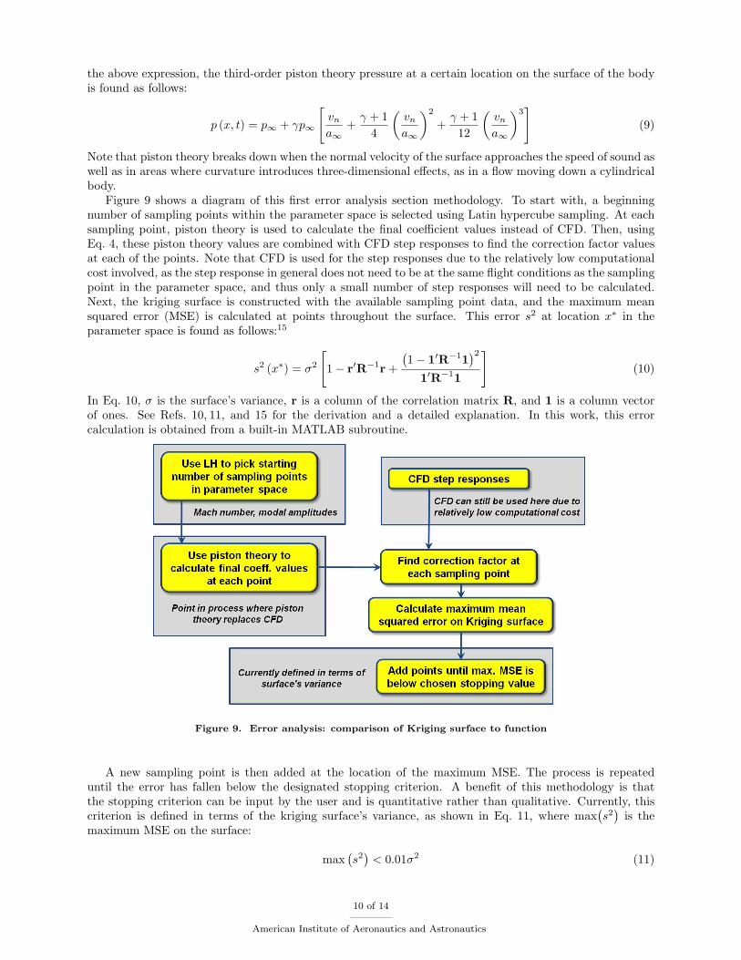
Figure 9 shows a diagram of this �rst error analysis section methodology. To start with, a beginningnumber of sampling points within the parameter space is selected using Latin hypercube sampling. At eachsampling point, piston theory is used to calculate the �nal coe�cient values instead of CFD. Then, usingEq. 4, these piston theory values are combined with CFD step responses to �nd the correction factor valuesat each of the points. Note that CFD is used for the step responses due to the relatively low computationalcost involved, as the step response in general does not need to be at the same ight conditions as the samplingpoint in the parameter space, and thus only a small number of step responses will need to be calculated.Next, the kriging surface is constructed with the available sampling point data, and the maximum meansquared error (MSE) is calculated at points throughout the surface. This error s2 at location x� in theparameter space is found as follows:15

s2 (x�) = �2

"1� r0R�1r +

�1� 10R�11

�210R�11

#(10)

In Eq. 10, � is the surface’s variance, r is a column of the correlation matrix R, and 1 is a column vectorof ones. See Refs. 10, 11, and 15 for the derivation and a detailed explanation. In this work, this errorcalculation is obtained from a built-in MATLAB subroutine.

Figure 9. Error analysis: comparison of Kriging surface to function

A new sampling point is then added at the location of the maximum MSE. The process is repeateduntil the error has fallen below the designated stopping criterion. A bene�t of this methodology is thatthe stopping criterion can be input by the user and is quantitative rather than qualitative. Currently, thiscriterion is de�ned in terms of the kriging surface’s variance, as shown in Eq. 11, where max

�s2�

is themaximum MSE on the surface:

max�s2�< 0:01�2 (11)

10 of 14


Figures 10 and 11 show a simple graphical example of this process. Five sampling points are at �rstselected to model the function y = (x� 2) (x� 4) (x� 9). The corresponding kriging �t and MSE plot areshown in Fig. 10. Then, the above process is applied, and the end result is shown in Fig. 11. Three moresampling points were added, and the function and kriging �t are indistinguishable in the plot.

(a) Kriging �t (b) Mean squared error

Figure 10. Kriging �t and MSE with initial sampling points

(a) Kriging �t (b) Mean squared error

Figure 11. Kriging �t and MSE, error criterion satis�ed

Using the stopping criterion detailed above, around 90 sampling points were necessary for the constructionof the kriging surface of the two-dimensional half-diamond airfoil with Mach number and each of the threemodal amplitudes as parameters. Latin hypercube test points were generated using MATLAB’s lhsdesignsubroutine;20 100; 000 iterations were used, and the sampling points with minimum correlation were chosen.Note that since the speci�c beginning sampling points will di�er, the exact number of points necessary toachieve the stopping criterion was slightly di�erent for each time the above process was repeated.

B. Error of Function Compared to Truth Model

Once the kriging surface has been constructed in such a way that it matches up well with the intendedfunction, it is necessary to evaluate how well the function itself represents the truth model. Fig. 12 showsthe overall process that has been implemented. As before, piston theory is utilized due to low computationalexpense.

The overall error is investigated by comparing ROM and truth model results over a large sample of testcases throughout the parameter space. To begin with, Latin hypercube sampling is used to pick points at

11 of 14


Figure 12. Error analysis: comparison of function to truth model

which to run sinusoidal test cases. In addition to Mach number and modal amplitudes, modal frequenciesare also included as variables. These test points are in general di�erent than the points used for krigingsurface construction. For this study, 1; 000 test points have been used. At each point, the the sinusoidalinput response is calculated in two di�erent ways: once using the ROM based on a CFD step response andpiston theory correction factor and once using straight piston theory. The straight piston theory result herereplaces the CFD model as the \truth" model for comparison. Finally, the error of ROM as compared topiston theory results is found for each run. The ROM methodology’s accuracy is assessed by calculating themean and standard deviation of the errors over all runs.

Table 3 shows the range of parameters used for this study as well as the speci�c parameters of the runwhich had the highest error (denoted as \Max. Error"). Fig. 13(a) shows a scatter plot of the errors ofeach run along with the mean and standard deviation superimposed on the plot, while Fig. 13(b) shows thecomparison of the ROM, piston theory, and CFD results for the maximum error case.

Table 3. Error analysis parameters

Parameter Min. Value Max. Value Max. ErrorM 5 9:5 8:56d1 �60� 60� �7:71�d2 �25� 25� �13:02�d3 �25� 25� 13:13�k1 0:028 0:375 0:168k2 0:028 0:375 0:044k3 0:028 0:375 0:059

In general, the errors are relatively small. The overall mean of the errors, denoted by the solid red line inthe �gure, is 8:89% with a standard deviation of 4:44%. The largest error, for which the ROM-truth modelcomparison is shown in Fig. 13(b), is just over 45%. For this case, piston theory shows a closer agreementwith the results than the ROM. For this geometry, piston theory has been shown to agree well with theCFD results in general. However, for more complex con�gurations, such as highly three-dimensional bodies,

12 of 14


(a) Error analysis results (b) Maximum error case

Figure 13. Results: comparison of function to truth model

piston theory will be expected to break down, whereas the ROM can be applied to any con�guration.The goal of this methodology is not to give an exact error that is expected to be incurred but rather a

general picture of the error. For the more complex geometries, where piston theory will not be expected togive as accurate of results, the use of piston theory and/or other simpli�ed models serve to give a picture ofthe general trends expected with the error, not a detailed accurate analysis of any speci�c errors seen.

VI. Concluding Remarks

A convolution-based reduced-order modeling methodology for the unsteady aerodynamics of a hypersonicvehicle has been extended from capturing single-modal oscillation e�ects to multiple-modal oscillations.Studies have looked at the error incurred as functions of increasing reduced frequency. An error estimationmethodology has been developed to investigate prior to model construction the general trends of the errorexpected to be encountered. This methodology includes a quanti�cation of the number of sampling pointsnecessary to construct the kriging surface as well as the use of simpli�ed models to replace CFD results. Forthe two-dimensional half-diamond airfoil geometry used in this work, the major conclusions are as follows:

� Errors were shown to increase with increased reduced frequency. However, they remained relativelysmall over the range considered.

� The multi-modal correction factor was successfully applied to this con�guration over a range of fre-quencies, modal oscillation amplitudes, and Mach numbers and showed improved agreement with CFDresults over straight superposition of individual modal responses.

� Using the error estimation methodology, the mean error over 1; 000 sample runs was found to be justunder 9% with a standard deviation of slightly over 4%.

Future work will consist of the application of the ROM to a three-dimensional rocket-type body where pistontheory will not be expected to provide as accurate of results. Also, the error quanti�cation results presentedabove are only valid for this speci�c con�guration and do not provide general error bounds for the method.Further investigations will explore these bounds in terms of geometry and the ROM methodology’s extensioninto other ight regimes.

Acknowledgments

Funds for the Michigan-AFRL Collaborative Center in Control Science (MACCCS) were made availablefrom the Air Force Research Laboratory/Air Vehicles Directorate grant number FA 8650-07-2-3744. Theprogram manager is Michael Bolender.

13 of 14


References

1Glaz, B., Liu, L., Friedmann, P., Bain, J., and Sankar, L., \A Surrogate Based Approach to Reduced-Order DynamicStall Modeling," Proceedings of the 51st AIAA/ASME/ASCE/AHS/ASC Structures, Structural Dynamics, and MaterialsConference, AIAA Paper No. 2010-3042, April 2010.

2Silva, W., \Recent Enhancements to the Development of CFD-Based Aeroelastic Reduced-Order Models," Proceedingsof the 48th AIAA/ASME/ASCE/AHS/ASC Structures, Structural Dynamics, and Materials Conference, AIAA Paper No.2007-2051, April 2007.

3Lind, R., Prazenica, R., Brenner, M., and Baldelli, D., \Identifying Parameter-Dependent Volterra Kernels to PredictAeroelastic Instabilities," AIAA Journal , Vol. 43, No. 12, December 2005, pp. 2496{2502.

4Baldelli, D., Zeng, J., Lind, R., and Harris, C., \Flutter-Prediction Tool for Flight-Test-Based Aeroelastic Parameter-Varying Models," Journal of Guidance, Control, and Dynamics, Vol. 32, No. 1, January-February 2009, pp. 158{171.

5Prazenica, R., Reisenthel, P., Kurdila, A., and Brenner, M., \Volterra Kernel Extrapolation for Modeling NonlinearAeroelastic Systems at Novel Flight Conditions," Journal of Aircraft , Vol. 44, No. 1, January-February 2007, pp. 149{162.

6Omran, A. and Newman, B., \Piecewise Global Volterra Nonlinear Modeling and Characterization for Aircraft Dynamics,"Journal of Guidance, Control, and Dynamics, Vol. 32, No. 3, May-June 2009, pp. 749{759.

7Skujins, T. and Cesnik, C., \Reduced-Order Modeling of Hypersonic Vehicle Unsteady Aerodynamics," Proceedings ofthe AIAA Atmospheric Flight Mechanics Conference, AIAA Paper No. 2010-8127, August 2010.

8Silva, W., \Discrete-Time Linear and Nonlinear Aerodynamic Impulse Responses for E�cient CFD Analyses," Ph.D.dissertation, College of William & Mary, December 1997.

9Fung, Y., An Introduction to the Theory of Aeroelasticity, Dover Publications, Mineola, New York, 1993.10Lophaven, S., Nielsen, H., and Sondergaard, J., \DACE: A MATLAB Kriging Toolbox, Version 2.0," Tech. Rep. IMM-

TR-2002-12, Informatics and Mathematical Modelling, Denmark, August 1, 2002.11Sacks, J., Welch, W., Mitchell, T., and Wynn, H., \Design and Analysis of Computer Experiments," Statistical Science,

Vol. 4, No. 4, 1989, pp. 409{435.12Rumsey, C. and Biedron, R., \CFL3D User’s Manual, Version 5.0, Second Edition," Tech. Rep. Hampton, VA, NASA

Langley Research Center, September 1997 (last updated August 2009).13Anon., \Documentation for ANSYS ICEM CFD 12.0," Tech. rep., ANSYS, Canonsburg, Pennsylvania, 2009.14Cioppa, T. and Lucas, T., \E�cient Nearly Orthogonal and Space-Filling Latin Hypercubes," Technometrics, Vol. 49,

No. 1, February 2007, pp. 45{55.15Jones, R., Schonlau, M., and Welch, W., \E�cient Global Optimization of Expensive Black-Box Functions," Journal of

Global Optimization, Vol. 13, No. 4, 1998, pp. 455{492.16Glaz, B., Friedmann, P., and Liu, L., \E�cient Global Optimization of Helicopter Rotor Blades for Vibration Reduction

in Forward Flight," Proceedings of the 11th AIAA/ISSMO Multidisciplinary Analysis and Optimization Conference, AIAAPaper No. 2006-6997, September 2006.

17Ashley, H. and Zartarian, G., \Piston Theory - A New Aerodynamic Tool for the Aeroelastician," Journal of the Aero-nautical Sciences, Vol. 23, No. 12, 1956, pp. 1109{1118.

18Lighthill, M., \Oscillating Airfoils at High Mach Number," Journal of the Aeronautical Sciences, Vol. 20, No. 6, 1953,pp. 402{406.

19McNamara, J. and Friedmann, P., \Aeroelastic and Aerothermoelastic Analysis of Hypersonic Vehicles: Current Statusand Future Trends," Proceedings of the 48th AIAA/ASME/ASCE/AHS/ASC Structures, Structural Dynamics, and MaterialsConference, AIAA Paper No. 2007-2013, April 2007.

20Anon., \MATLAB Version 7.10.0 User Guide," Tech. rep., The MathWorks, Inc., Natick, MA, 2010.

14 of 14


Documents

Reduced-Order Modeling of Hypersonic Unsteady … · Reduced-Order Modeling of Hypersonic Unsteady Aerodynamics Due to ... This is not intended to be representative of any speci c