arX

iv:1

504.

0472

7v2

[qu

ant-

ph]

17

Dec

201

5

Reducing Computational Complexity of Quantum Correlations

Titas Chanda, Tamoghna Das, Debasis Sadhukhan, Amit Kumar Pal, Aditi Sen(De), and Ujjwal SenHarish-Chandra Research Institute, Chhatnag Road, Jhunsi, Allahabad - 211019, India

We address the issue of reducing the resource required to compute information-theoretic quantumcorrelation measures like quantum discord and quantum work deficit in two qubits and higherdimensional systems. We show that determination of the quantum correlation measure is possibleeven if we utilize a restricted set of local measurements. We find that the determination allows us toobtain a closed form of quantum discord and quantum work deficit for several classes of states, witha low error. We show that the computational error caused by the constraint over the complete set oflocal measurements reduces fast with an increase in the size of the restricted set, implying usefulnessof constrained optimization, especially with the increase of dimensions. We perform quantitativeanalysis to investigate how the error scales with the system size, taking into account a set of plausibleconstructions of the constrained set. Carrying out a comparative study, we show that the resourcerequired to optimize quantum work deficit is usually higher than that required for quantum discord.We also demonstrate that minimization of quantum discord and quantum work deficit is easier inthe case of two-qubit mixed states of fixed ranks and with positive partial transpose in comparisonto the corresponding states having non-positive partial transpose. Applying the methodology toquantum spin models, we show that the constrained optimization can be used with advantage inanalyzing such systems in quantum information-theoretic language. For bound entangled states, weshow that the error is significantly low when the measurements correspond to the spin observablesalong the three Cartesian coordinates, and thereby we obtain expressions of quantum discord andquantum work deficit for these bound entangled states.

I. INTRODUCTION

Entanglement [1] as a measure of quantum correla-tions existing between subsystems of a composite quan-tum system has been shown to be indispensable in per-forming several quantum information tasks [2, 3]. Todeal with challenges such as decoherence due to system-environment interaction, entanglement distillation proto-cols [4] to purify highly entangled states from a collectionof states with relatively low entanglement have also beeninvented. Parallely, various counter-intuitive findings suchas substantial non-classical efficiency of quantum stateswith vanishingly small entanglement, and locally indistin-guishable orthogonal product states [5–8] have motivatedthe search for quantum correlations not belonging to theentanglement-separability paradigm. This has led to thepossibility of introducing more fine-grained quantum cor-relation measures than entanglement, such as quantumdiscord (QD) [9], quantum work deficit (QWD) [10], andvarious ‘discord-like’ measures [11, 12], opening up a newdirection of research in quantum information theory. Al-though establishing a link between the measures of quan-tum correlations belonging to the two different genres hasalso been tried [13], a decisive result is yet to be found inthe case of mixed bipartite quantum states. Note, how-ever, that all these measures reduce to von Neumann en-tropy of local density matrix for pure states. In recentyears, the interplay between entanglement distillation andquantum correlations such as QD and QWD has been un-der focus [14]. However, proper understanding of the re-lation between such measures and distillable as well asbound entanglement [15–21] is yet to be achieved.There has been a substantial amount of work in deter-

mining QD for various classes of bipartite as well as multi-

partite mixed quantum states [22–24]. A common obser-vation that stands out from these works is the computa-tional complexity of the task, due to the optimization overa complete set of local measurements involved in its def-inition [9]. For general quantum states, the optimizationis often achieved via numerical techniques. It has recentlybeen shown that the problem of computing quantum dis-cord is NP-complete, thereby making the quantity compu-tationally intractable [25]. The lack of a well-establishedanalytic treatment to determine QD has also restrictedthe number of experiments in this topic [26]. Despite con-siderable efforts to analytically determine QD for generaltwo-qubit states [22, 23], a closed form expression existsonly for the Bell diagonal (BD) states [22].

A number of recent numerical studies have shown thatfor a large fraction of a very special class of two-qubitstates, QD can always be calculated by performing theoptimization over only a small subset of the complete setof local projection measurements [27, 29], thereby reduc-ing the computational difficulty to a great extent. Thesestates are constructed of the three diagonal correlators ofthe correlation matrix, and any one of the three magneti-zations, which is similar for both the qubits. The subset,in the present case, consists of the projection measure-ments corresponding to the three Pauli matrices, σx, σy,and σz. Curiously, the assumption that QD can be opti-mized over this subset for the entire class of such statesresults only in a small absolute error in the case of thosestates where the assumption is not valid [27, 29]. Thisproperty also allows one to determine closed form for QDfor the entire class of such two-qubit states within themargin of small absolute error in calculation [27–29].

Optimization over such a small subset of the completeset of local projection measurements is logical in the situ-

2

ations where a constraint over the allowed local measure-ments is at work. The knowledge of such a subset may beimportant in quantum estimation theory [30], in relationto quantities that are non-linear functions of the quantumstates, such as the QD, where estimation of the parametervalues to determine the optimal projection measurementdepends on the the number of measurements required toobtain the desired quantity within a manageable range oferror. Also, the existence of such subsets has the potentialto be operationally as well as energetically advantageousin experimental determination of the QD and similar mea-sures for a given quantum state. However, the investiga-tion of the existence of such special subsets of allowedlocal projectors in the computation of quantum correla-tions like QD and QWD, as of now, are confined onlyto special classes of quantum states in C2 ⊗ C2 systems[27–29]. A natural question that arises is whether suchsubsets of local projectors can exist for general bipartitequantum states. The possible scaling of the absolute er-ror resulting from the limitation on the number of allowedlocal projectors in the subset is also an interesting issue.In this paper, we investigate the issue of simplifying

the optimization of quantum correlation measures like QDand QWD in the case of general two-qubit mixed states ofdifferent ranks with positive as well as non-positive par-tial transpose (NPPT) [31] by using a restricted set oflocal projection measurements. We provide a mathemati-cal description of the optimization of quantum correlationmeasures over a restricted set of allowed local projectionmeasurements, and discuss the related statistics of com-putational error. Using a set of plausible definitions of therestricted set, we show that the absolute error, resultingdue to the constraint over the set of projectors, dies outconsiderably fast. Using the scaling of the error with thesize of the restricted subset, we demonstrate that even asmall number of properly chosen projectors can form a re-stricted set leading to a very small absolute error, therebymaking the computation of quantum correlation measuresconsiderably easier.Our method also helps us to find expressions with negli-

gible error for QD and QWD of several important classesof quantum states. We demonstrate this in the case oftwo-qubit “X” states [32], which occur, in general, inground or thermal states of several quantum spin mod-els. Hence, our approach provides a way to study co-operative phenomena present in such systems with lessnumerical difficulty, as demonstrated here for anisotropicXY model in the presence of external transverse field [33].We extend the study to the paradigmatic classes of boundentangled (BE) states, where the computation of QD andQWD using a special restricted subset is discussed, andtheir analytic forms with small error are determined. Theresults indicate that the error resulting from the restrictedmeasurement in the case of states with positive partialtranspose (PPT) is less compared to the states with non-positive partial transpose (NPPT). Such constrained op-timizations can be a powerful tool to study physical quan-tities in higher dimensions, and to obtain closed forms of

QD and QWD.The paper is organized as follows. In Sec. II, we provide

a mathematical description of the computation of quan-tum correlation measures by performing the optimizationover a constrained set of local projection measurements,defining the corresponding absolute error in calculation.In Sec. III, we discuss a set of constructions of the subsetin relation to the statistics of the error for general two-qubit mixed states in the state space. We also consider ageneral two-qubit state in the parameter space, and showhow symmetry of the state helps in defining the restrictedsubset. We demonstrate how our method can be usedto determine closed form expressions of quantum corre-lation measures, and comment on the applicability of themethod in real physical systems like quantum spin models.In particular, we show that the constrained optimizationtechnique performs quite well in analyzing the anisotropicXY model in transverse field in terms of quantum corre-lation measures. In Sec. IV, the results on the quantumcorrelations in BE states are presented. Sec. V containsthe concluding remarks.

II. DEFINITIONS AND METHODOLOGY

In this section, after presenting an overview of the quan-tum correlation measures used in this paper, namely, QDand QWD, we introduce the main concepts of the paper,i.e., constrained QD as well as QWD by restricting theoptimization over a small subset of the complete set ofallowed local measurements. We also discuss the corre-sponding error generated due to the limitation in mea-surements.

A. Quantum discord

For a bipartite quantum state ρAB, the QD is definedas the minimum difference between two inequivalent defi-nitions of the quantum mutual information. While one ofthem, given by I(ρAB) = S (ρA)+S (ρB)−S (ρAB), can beidentified as the “total correlation” of the bipartite quan-tum system ρAB [34], the other definition takes the formJ→(ρAB) = S (ρB)−S (ρB|ρA), which can be argued as ameasure of classical correlation [9]. Here, ρA and ρB arelocal density matrices of the subsystems A and B, respec-tively, S (ρ) = −Tr [ρ log2 ρ] is the von Neumann entropyof the quantum state ρ, and S(ρB |ρA) =

∑

k pkS(

ρkAB

)

is the quantum conditional entropy with

ρkAB =(

ΠAk ⊗ IB

)

ρAB

(

ΠAk ⊗ IB

)

/pk, (1)

and

pk = Tr[(

ΠAk ⊗ IB

)

ρAB

]

. (2)

The subscript ‘→’ implies that the measurement, rep-resented by a complete set of rank-1 projective opera-tors, {ΠA

k }, is performed locally on the subsystem A,

3

and IB is the identity operator defined over the Hilbertspace of the subsystem B. The QD is thus quantified asD = min{I(ρAB)− J→(ρAB)}, where the minimization isperformed over the set SC , the class of all complete setsof rank-1 projective operators. One must note here theasymmetry embedded in the definition of the QD over theinterchange of the two subsystems, A and B. Throughoutthis paper, we calculate QD by performing local measure-ment on the subsystem A.

B. Quantum work deficit

Along with the QD, we also consider the QWD [10]of a quantum state, defined as the difference betweenthe amount of extractable pure states under suitably re-stricted global and local operations. In the case of a bipar-tite state ρAB, the class of global operations, consistingof (i) unitary operations, and (ii) dephasing the bipartitestate by a set of projectors, {Πk}, defined on the Hilbertspace H of ρAB, is called “closed operations” (CO) underwhich the amount of extractable pure states from ρAB isgiven by ICO = log2 dim (H) − S(ρAB). And, the classof operations consisting of (i) local unitary operations,(ii) dephasing by local measurement on the subsystem A,and (iii) communicating the dephased subsystem to theother party, B, over a noiseless quantum channel is theclass of “closed local operations and classical communi-cation” (CLOCC), under which the extractable amountof pure states is ICLOCC = log2 dim (H) − minS (ρ′AB).Here, ρ′AB =

∑

k pkρkAB is the average quantum state af-

ter the projective measurement {ΠAk } has been performed

on A, with ρkAB and pk given by Eqs. (1) and (2), re-spectively. The minimization in ICLOCC is achieved overSC . The QWD, W , is given by the difference between thequantities ICO (ρAB) and ICLOCC (ρAB).

C. Constrained Quantum Correlations: Error inEstimation

We now introduce the physical quantity, which will helpus to reduce the computational complexity involved inevaluation of QD and QWD. In particular, we considerthe bipartite quantum correlations in the scenario wherethere are restrictions on the complete set of projectorsdefining the local measurement on one of the subsystems.Let us assume that constraints on the local measurementrestrict the class of projection measurements to a subsetSE (SE ⊆ SC), where there are n sets of projection mea-surements in SE . Performing the optimization only overthe set SE , a “constrained” quantum correlation (CQC),Qc, can be defined. We call the subset SE as the “ear-marked” set. Let the actual value of a given quantumcorrelation measure, Q, for a fixed bipartite state, ρAB,be Qa. If the definition of Q involves a minimization,log2 d ≥ Qc ≥ Qa, while a maximization in the definitionleads to log2 d ≥ Qa ≥ Qc, where d is the minimum of the

dimensions among the two parties making up the bipar-tite state and where we have assumed that log2 d is themaximum value of Qa or Qc. For example, one can definethe constrained QD (CQD) as

Dc = minSDE

[I(ρAB)− J→(ρAB)], (3)

while the constrained QWD (CQWD) is given by

Wc = minSWE

[S(ρ′AB)− S(ρAB)]. (4)

Note that in general, the earmarked sets for QD andQWD, represented by SD

E and SWE respectively, may not

be identical.

Evidently, the actual projector for which the quantumcorrelation is optimized may not belong to SE . Therefore,restricting the optimization over the earmarked set givesrise to error in estimation of the value of Q for a fixedquantum state, ρAB. Let us denote the absolute erroroccurring due to the optimization over SE , instead of SC ,for an arbitrary bipartite state ρAB, by ε, where

εn = |Qc −Qa|, (5)

with log2 d ≥ εn ≥ 0. We call this error as the “volun-tary” error (VE). One must note that the VE depends onthe size of the earmarked set, n, as well as the distributionof the elements of SE in the space of projection measure-ments. When n→ ∞, we may (but not necessarily) haveSE → SC , resulting in Qc → Qa, whence VE vanishes.However, for a finite value of n, we denote the VE by εn.Note that εn also depends on the actual form of the nprojection measurements in SE . If ε = 0 for a quantumstate even when the optimization is performed over theset SE , we call the quantum state an “exceptional” state.

Apart from the quantum information-theoretic mea-sures having entropic definitions, such as QD and QWD,there exists a variety of geometric measures of “discord-like” quantum correlations. These measures are basedon different metrics quantifying the minimum distance ofthe quantum state from the set of all possible classical-quantum states [8, 35–40]. Although a collection of dis-tance metrics have been used to characterize geometricmeasures of quantum correlations, it has been shown thatout of all the Schatten p-norm distances, only the one-norm distance has properties that are rather similar tothe QD as well as QWD [38–40]. But due to the diffi-culty in optimizing the measure, analytically closed formsof one-norm geometric discord has been obtained only forsome special types of states, e.g., Bell diagonal states, andthe X states [40]. Our methodology, along with the tradi-tional QD and QWD, is applicable also to the geometricmeasures that require an optimization. Motivated by theusefulness of QD and QWD in certain quantum proto-cols [5–7, 41], we choose these measures for the purposeof demonstration.

4

III. TWO-QUBIT SYSTEMS

In the case of a C2A ⊗ C2

B system where each of thesubsystems consists of a single qubit only, the rank-1 pro-jection measurements are of the form {ΠA

k = U |k〉〈k|U †,|k〉 = |0〉, |1〉}, where U , a local unitary operator in SU(2),can be parametrized using two real parameters, θ, and φ,as

U =

(

cos θ2 sin θ

2eiφ

− sin θ2e

−iφ cos θ2

)

. (6)

Here, 0 ≤ θ ≤ π, 0 ≤ φ < 2π, and {|0〉, |1〉} denotesthe computational basis in C2. Note that θ and φ can beidentified as the azimuthal and the polar angles, respec-tively, in the Bloch sphere representation of a qubit. Letus define a parameter transformation, fθ = cos θ, so that−1 ≤ fθ ≤ 1. Here and throughout this paper, when-ever we need to perform an optimization over all rank-1projection measurements on a qubit to evaluate a givenquantum correlation, Q, we choose the parameters fθ andφ uniformly in [−1, 1] and [0, 2π] respectively. An ear-marked set, in the present case, is equivalent to a subsetof the complete set of allowed values of fθ and φ.

A. Mixed states with different ranks

First, we discuss the case of general two-qubit mixedstates of different ranks. As described above, an optimalset of (fθ, φ) values define the optimal projection measure-ment for the computation of the fixed quantum correlationmeasure, Q. Let us consider the probability, pr, that theoptimal values of the real parameters, fθ and φ, for a fixedmeasure of quantum correlation, Q, of a randomly chosentwo-qubit mixed state of rank r, lie in (fθ, fθ + dfθ), and(φ, φ + dφ), respectively. The fact that the real param-eters, fθ and φ, are independent of each other suggeststhat

pr = Pr(fθ, φ)dfθdφ = P 1r (fθ)dfθP

2r (φ)dφ, (7)

which allows one to investigate the two probability den-sity functions (PDFs), P 1

r (fθ), and P2r (φ), independently.

Here, P 1r (fθ)dfθ denotes the probability that irrespective

of the optimal value of φ, the optimal value of fθ lies be-tween fθ and fθ + dfθ for the fixed quantum correlationmeasure, Q, calculated for a two-qubit mixed quantumstate of rank r. A similar definition holds for the proba-bility P 2

r (φ)dφ also.In the case of two-qubit systems, an uniform distri-

bution of the projection measurements in the measure-ment space corresponds to the uniform distribution of the(fθ, φ) points on the surface of the Bloch sphere. It is,therefore, reasonable to expect that the PDFs, P 1

r (fθ)dfθand P 2

r (φ)dφ, correspond to uniform distributions over theallowed ranges of values of fθ and φ. To verify this numer-ically, we consider QD and QWD as the chosen measuresof quantum correlation. The corresponding P 1

r (fθ), and

P 2r (φ) in the case of two-qubit mixed states having NPPT

or having PPT for both QD and QWD are determined bygenerating 5× 105 states Haar uniformly for each value ofr = 2, 3, and 4. We find that in the case of QD as well asQWD, both P 1

r (fθ), and P2r (φ) are uniform distributions

over the entire ranges of corresponding parameters, fθ andφ, irrespective of the rank of the state as well as whetherthe state is NPPT or PPT. Note here that for two-qubitmixed states of rank-2, almost all states are NPPT whilethe PPT states form a set of measure zero [42], whichcan also be verified numerically. However, in the case ofr = 3 and 4, non-zero volumes of PPT states are found.In C2 ⊗ C2 systems, all NPPT states are entangled whilePPT states form the set of separable states [43].The fact that all the rank-1 projection measurements

are equally probable makes the qualitative features of Qc

depend only on the geometrical structure of the earmarkedset, SE , and not on the actual location of the elements ofthe set on the Bloch sphere. In the following, we considerfour distinct choices of the set SE for both QD and QWDin the case of two-qubit mixed states with ranks r = 2, 3, 4,and discuss the corresponding scaling of the average VE.

Case 1: SE with (fθ , φ) distributed over a circle on theBloch sphere

We start by constructing the earmarked set with projec-tion measurements such that the corresponding (fθ, φ) lieson the circle of intersection of a fixed plane with the Blochsphere. Let us assume that the corresponding VE result-ing from the restricted optimization of Q, for an arbitrarytwo-qubit mixed state of rank r is given by εrn, n being thesize of SE , and where the corresponding n points on thecircle are symmetrically placed. Let us also assume thatthe CQC calculated by constrained optimization over theset SE with n→ ∞ is given by Q′

c and the correspondingVE, called the “asymptotic error”, is εr∞ = |Q′

c − Qa|.To investigate how fast εrn reaches εr∞ on average withincreasing n, one must look into the variation of εrn − εr∞against n for different values of r. Here, εrn is the averagevalue of the VE, εrn, and is given by

εrn =

∫ 1

0

εrnPrn(ε

rn)dε

rn, (8)

with P rn(ε

rn)dε

rn being the probability that for an arbitrary

two-qubit mixed state with rank r, the VE lies betweenεrn and εrn + dεrn when Qc is calculated over SE of size ndefined on the chosen plane. A similar definition holds forthe average asymptotic VE, εr∞, and the PDF, P r

∞(εr∞),in the limit n→ ∞, where

εr∞ =

∫ 1

0

εr∞Pr∞(εr∞)dεr∞. (9)

We consider two different ways in which the plane ischosen. (a) We fix a value of fθ = f ′

θ such that thecorresponding states on the Bloch sphere are given by

5

(a) (b)

Figure 1. (Color online.) (a) Schematic representation of theearmarked set confined on the circle defined by the intersectionof the (x, y) plane, fixed by fθ = 0, and the Bloch sphere. Theplane is specified by the eigenbases of σx and σy. (b) Schematicrepresentation of the earmarked set confined on a set of circles,defined by the intersections of a set of planes and the Blochsphere. The planes are considered to be symmetrically placedon either side of the (x, y) plane fixed by fθ = 0.

|ξ〉 = coscos−1 f ′

θ

2 |0〉 + eiφ sincos−1 f ′

θ

2 |1〉, where φ acts asthe spanning parameter. (b) In the second option, we fixthe value of φ = φ′ while vary fθ with the correspondingstates |ξ〉. We consider both the scenarios, and investigatethe scaling of the corresponding average VEs for both QDand QWD for arbitrary two-qubit mixed states of differentranks.(a) Fixed value of fθ: Unless otherwise stated, here andthroughout this paper, we shall fix a plane by assigning avalue to fθ. For the purpose of demonstration, we choosefθ = 0, fixing the (x, y) plane defined by the eigenbasis ofthe Pauli matrices σx and σy, where an arbitrary projec-tion basis can be written as |ξ〉 = 1√

2(|0〉 + eiφ|1〉). The

earmarked set of size n on the perimeter of the circle of in-tersection of the (x, y) plane and the Bloch sphere can begenerated by a set of n projectors of the form U |k〉〈k|U †,|k〉 = |0〉, |1〉, obtained by using a fixed fθ = 0, and n eq-uispaced divisions of the entire range of φ. Here, the formof U is given in Eq. (6). The situation is depicted in Fig.1(a). To determine the PDFs, P r

n(εrn) and P r

∞(εr∞), weHaar uniformly generate 5× 105 random two-qubit mixedstates of rank r = 2, 3, and 4 each. The correspondingaverage VE, εrn, and average asymptotic VE, εr∞, in thecase of both QD and QWD are determined using Eqs. (8)and (9) respectively. For both the quantum correlationmeasures, the quantity εrn − εr∞ is found to have a power-law decay with the size, n, of the earmarked set, on thelog-log scale for all values of r. One can determine thefunctional dependence of εrn over n as

εrn = εr∞ + κn−τ , (10)

where the fitting constant, κ, and the scaling exponent, τ ,are estimated from the numerical data. Fig. 2 shows thevariations of εrn−εr∞ with n for both QD and QWD in thecase of rank-2 two-qubit states. The insets in Fig. 2 showsthe corresponding variations of εrn− εr∞ with increasing nin the log-log scale.

QDr NPPT PPT

3

κ = 1.45× 10−1 ± 9.97 × 10−3

τ = 1.93± 1.05× 10−2

εr=3∞

= 9.56× 10−2

κ = 1.04× 10−1 ± 7.10× 10−2

τ = 1.94 ± 1.01× 10−2

εr=3∞

= 6.98× 10−2

4

κ = 1.21× 10−1 ± 8.32 × 10−3

τ = 1.94± 1.02× 10−2

εr=4∞

= 7.80× 10−2

κ = 8.67× 10−2 ± 5.96× 10−3

τ = 1.94 ± 9.90× 10−3

εr=4∞

= 5.78× 10−2

QWDr NPPT PPT

3

κ = 1.89× 10−1

± 1.30 × 10−2

τ = 1.93± 1.13× 10−2

εr=3∞

= 1.18× 10−1

κ = 1.52× 10−1

± 1.04× 10−2

τ = 1.93 ± 1.08× 10−2

εr=3∞

= 9.64× 10−2

4

κ = 1.50× 10−1

± 1.03 × 10−2

τ = 1.93± 1.07× 10−2

εr=4∞

= 9.23× 10−2

κ = 1.20× 10−1

± 8.26× 10−3

τ = 1.94 ± 1.04× 10−2

εr=4∞

= 7.52× 10−2

Table I. Values of the fitting constant, κ, scaling exponent,τ , and asymptotic error, εr

∞in the case of NPPT as well as

PPT two-qubit mixed states of rank r = 3 and 4. Here, QDand QWD are considered as quantum correlation measures,and the earmarked set is fixed on the circle defined by theintersection of a plane fixed by fθ = 0, and the Bloch sphere.The corresponding power-law variations of εr=2

n − εr=2

∞with n

are depicted in Fig. 3.

0

0.05

0.1

0.15

0.2

0.25

0.3

5 10 15 20 25 30 35 40 45 50

– εr=2

n

− – εr=

2∞

n

QD-numericalQD-fitted

QWD-numericalQWD-fitted

10-4

10-3

10-2

10-1

2 5 10 20 50 1

Figure 2. (Color online.) Variation of εr=2

n −εr=2

∞as a function

of n in the case of QD and QWD. (Inset) Linear variation ofεr=2

n − εr=2

∞as a function of n in the log-log graph for QD

and QWD, where the variation is given by Eq. (10). Thenumerical data is represented by points while the fitted curveis given by solid lines. The fitting parameters are estimated asκ = 1.77 × 10−1 ± 1.22 × 10−2, and τ = −1.92 ± 1.11 × 10−2

with εr=2

∞= 1.21× 10−1 in the case of QD, whereas for QWD,

κ = 2.58 × 10−1 ± 1.78 × 10−2, τ = −1.91 ± 1.23 × 10−2,and εr=2

∞= 1.66 × 10−1. In the main figure, the abscissa is

dimensionless, while the quantities εr=2

n and εr=2

∞are in bits. In

the inset, the ordinate is in the natural logarithm of εr=2

n −εr=2

∞,

and the x axis is in the natural logarithm of n.

6

The variations of εrn − εr∞ with n in the log-log scaleusing both QD and QWD with NPPT as well as PPTtwo-qubit mixed states of rank r = 3 and r = 4 are shownseparately in Fig. 3. The corresponding exponents andfitting parameters are quoted in Table I. Note that al-though the exponent, τ , in the case of QD and QWD hasequal values up to the first decimal point for all the cases(for NPPT and PPT states with different ranks), the av-erage asymptotic VE, εr∞, is larger in the case of QWDin comparison to that for QD. This is reflected in the factthat the graph for QWD is above the graph for QD, asshown in Fig. 2 and 3. Note also that εrn is less in thecase of PPT states than the NPPT states, when two-qubitstates of a fixed rank are considered.Note that in the above example, we have fixed the plane

by fixing fθ = 0, which corresponds to a great circle onthe Bloch sphere. One can also fix a great circle on theBloch sphere by fixing any value of φ in its allowed rangeof values. Earmarked sets defined over any such great cir-cle on the Bloch sphere have similar scaling properties ofthe average VE as long as the points corresponding to theprojection measurements belonging to the set SE are dis-tributed uniformly over the circle. However, for differentdistribution, one can obtain different scaling exponentsand fitting parameters. We shall shortly discuss one suchexample.For fθ 6= 0, smaller circles over the Bloch spheres are

obtained. One can also investigate the scaling behaviourof the average VE in the case of earmarked sets havingelements corresponding to points distributed over thesesmaller circles by using φ as the spanning parameter.However, different values for the scaling exponents andfitting parameters are obtained as |fθ| → 1.(b) Fixed value of φ: Next, we consider the scenariowhere the distribution of the (fθ, φ) points correspondingto the projection measurements constituting the set SE onthe circle of our choice is different (i.e., non-uniform) thanthe previous example. This may happen due to restric-tions imposed by apparatus during experiment, or otherrelevant physical constraints. As before, we choose theplane by fixing φ = 0, thereby confining the earmarkedset on the great circle representing the intersection of the(x, z) plane defined by the eigenbases of σx and σz , andthe Bloch sphere. However, to demonstrate the effect ofsuch non-uniformity over the scaling parameters, we con-sider the (fθ, φ) points corresponding to the n elements inSE by n equal divisions of the entire range of fθ. Note thatthe current choice of fθ as the spanning parameter leadsto a different (non-uniform) distribution of the points cor-responding to the projection measurements in SE on thechosen circle.Similar to the previous case of fθ = 0, one can also

study the scaling of average VE by defining εrn and εr∞ cor-responding to the present case. The variation of εrn − εr∞with n, as in the previous case, is given by Eq. (10), onlywith different values of fitting constant, scaling exponent,and average asymptotic error. In the case of two-qubitmixed states of rank-2, the appropriate parameter values

QDr NPPT PPT

3

κ = 1.04× 10−1 ± 5.60× 10−4

τ = 1.47± 1.70× 10−3

εr=3∞

= 9.54× 10−2

κ = 7.68× 10−2 ± 4.3× 10−4

τ = 1.48± 1.80× 10−3

εr=3∞

= 6.95× 10−2

4

κ = 8.95× 10−2 ± 9.6× 10−4

τ = 1.48± 3.4× 10−3

εr=3∞

= 7.81× 10−2

κ = 6.23× 10−2 ± 2.8× 10−4

τ = 1.48± 1.4× 10−3

εr=4∞

= 5.79× 10−2

Table II. Values of the fitting constant, κ, scaling exponent, τ ,and asymptotic error, εr

∞in the case of NPPT as well as PPT

two-qubit mixed states of rank r = 3 and 4. Here, quantumcorrelation is quantified by QD, and the earmarked set is fixedon the circle of intersection of a plane fixed by φ = 0, and theBloch sphere. The n points corresponding to the projectionmeasurements in SE are distributed over the circle by takinginto account n equispaced division of the range [−1, 1] of thespanning parameter fθ.

for QD are found to be κ = 1.30 × 10−1 ± 1.08 × 10−3,τ = 1.47 ± 2.7 × 10−3, with εr=2

∞ = 1.21 × 10−1. In thecase of states with r = 3 and 4, the values of κ, τ , and εr∞in the case of QD are tabulated in Table II. Note that thescaling exponents are different from those found in case ofa fixed fθ. However, the fact that the average asymptoticVE is less in the case of PPT states compared to thatof NPPT states remains unchanged even in the presentscenario.

One can carry out similar investigation taking QWDas the chosen measure of quantum correlation. As in theprevious case where fθ = 0, here also the exponent in thecase of QWD is found to be same with that for QD up tothe first decimal place, although the average asymptoticerror is higher.

Case 2: SE with (fθ , φ) on a collection of circles on theBloch sphere

We now consider the situation where the projectionmeasurements in the earmarked set are such that the cor-responding (fθ, φ) are not confined on the perimeter of asingle fixed disc only, but are lying on the perimeters of aset of fixed discs (Fig. 1(b)). As discussed earlier, thereare several ways in which a disc in the state space can befixed. For the purpose of demonstration, we achieve thisby fixing the value of fθ. The size, n, of the set SE , de-pends on two quantities: (i) the number, n1, of divisionsof the allowed range of φ on any one of the discs, and(ii) the number, n2, of discs that are considered for con-structing the earmarked set. Evidently, n = n1n2. Notethat the value of n1 is assumed to be constant for everydisc, although one may consider, in principle, a varyingnumber, ni

1, such that n =∑n2

i=1 ni1.

We demonstrate the situation with an example wherean arbitrary disc is fixed by fθ = f ′

θ, and a collection ofadditional discs positioned symmetrically with respect tothe fixed disc is considered. The fact that the number

7

10-4

10-3

10-2

10-1

2 5 10 20 50 1

– εr=3

n −

– εr=3

∞

n

Rank 3 PPT

(a) (b)

QD-numericalQD-fitted

QWD-numericalQWD-fitted

10-4

10-3

10-2

10-1

2 5 10 20 50 1

– εr=3

n −

– εr=3

∞

n

Rank 3 NPPT

QD-numericalQD-fitted

QWD-numericalQWD-fitted

10-4

10-3

10-2

10-1

2 5 10 20 50 1

– εr=4

n −

– εr=4

∞

n

Rank 4 PPT

(c) (d)

QD-numericalQD-fitted

QWD-numericalQWD-fitted

10-4

10-3

10-2

10-1

2 5 10 20 50 1

– εr=4

n −

– εr=4

∞

n

Rank 4 NPPT

QD-numericalQD-fitted

QWD-numericalQWD-fitted

Figure 3. (Color online.) Variations of εrn − εr∞

as a function of n, in log-log scale, for r = 3 and 4 in the case of NPPT andPPT two-qubit mixed states using QD and QWD. The numerical data is represented by points while the fitted curve is given bysolid lines. The corresponding values of the fitting constant, k, scaling exponent, τ , and asymptotic error, εr

∞, are tabulated in

Table I. The ordinates of all the figures are in natural logarithm of εrn − εr∞, with εrn and εr

∞individually being in bits, while the

abscissa is in natural logarithm of the cardinality of the earmarked set.

n2 includes the fixed disc itself implies that n2 is alwaysan odd number. In particular, the discs defining the setSE can be marked with different values of fθ, given byf jθ = f ′

θ±jh, where 0 ≤ j ≤ (n2−1)/2, and h = 2/(n2−1).The set SE , in the present case, approaches the complete

QD QWDr NPPT PPT

2n1 = 7n2 = 9 –

3n1 = 6n2 = 8

n1 = 5n2 = 7

4n1 = 5n2 = 8

n1 = 5n2 = 6

r NPPT PPT

2n1 = 9n2 = 11 –

3n1 = 7n2 = 10

n1 = 6n2 = 9

4n1 = 6n2 = 9

n1 = 5n2 = 8

Table III. Values of n1 and n2 that are sufficient to obtain avalue of average VE of the order of 10−3 in the case of NPPTand PPT two-qubit mixed states of different ranks, r, for QDand QWD. The values correspond to the case where the ear-marked set is confined on the surface of the Bloch sphere. Thecorresponding depiction is available in Fig. 5.

set of rank-1 projectors, SC , when both n1 and n2 tendto infinity. Similar to the previous case, one can studythe variation of average VE with the increase in the size,n, of the set SE . However, unlike the previous case, inthe situation where n→ ∞ is consequent to (fθ, φ) corre-sponding to the earmarked set being distributed over theentire Bloch sphere, the average asymptotic error, εr∞ = 0for all quantum correlation measures, since Qc → Qa insuch cases.

Fixing n1 to be a number for which the average VEcalculated over an arbitrary disc in the set is considerablysmall, variation of the average VE, εrn, with increasing n2,where n = n1n2, can be studied for QD and QWD. Here,the average is computed in a similar fashion as given inEq. (8). However, P r

n(εrn), in the present case, is obtained

by performing optimization of the corresponding quantumcorrelation measure using the current definition of SE .We fix f ′

θ = 0, and observe that in the case of QD, theaverage VE decreases linearly with increasing n2 for allvalues of n1 (See Fig. 4). This implies that for a fixed

8

0.04

0.06

0.08

0.1

0.12

0.14

5 10 15 20 25 30

– ε nr

n2

Rank 2Rank 3, NPPTRank 3, PPTRank 4, NPPTRank 4, PPT

Figure 4. (Color online.) Linear variation of εrn as a functionof n2 with n1 = 10 (n = n1n2) for QD. The earmarked set,in this case, is chosen on the perimeters of a set of discs inthe Bloch sphere, starting from the disc fixed by fθ = 0, andplacing the additional discs symmetrically on either side ofthe fθ = 0 disc. The numerical data obtained in each case isfitted to a straight line, εrn = mn2 + c. The fitting parametervalues are (i) m = −1.10 × 10−3, c = 0.12 (rank-2 states), (ii)m = −8.59× 10−4, c = 9.7× 10−2 (rank-3 NPPT states), (iii)m = −6.29 × 10−4, c = 7.14 × 10−2 (rank-3 PPT states), (iv)m = −6.99×10−4, c = 7.96×10−2 (rank-4 NPPT states), and(v) m = −5.22 × 10−4, c = 5.90 × 10−2 (rank-4 PPT states).The abscissa is dimensionless, while the quantity εrn is in bits.

n1, the spanning of the surface of the Bloch sphere by theperimeters of the discs in the set starting from fθ = 0occurs linearly with an increase in the value of n2. Fig. 4depicts the variation of the average VE, εrn, as a functionof n2 for n1 = 10, where the linear nature of the variationis clearly shown. Similar results hold in the case of QWDalso.

Case 3: SE with (fθ , φ) on the surface of Bloch sphere

Let us now consider the situation where the bases inSE are such that the corresponding (fθ, φ) are uniformlyscattered over the entire surface of the Bloch sphere sothat only n1 and n2 equal divisions of the entire range of fθand φ, respectively, are allowed, leading to an earmarkedset of size n = n1n2. Similar to the previous case, SE →SC , and ε

r∞ → 0 when both n1 and n2 approach infinity.

The average error, εrn, in the present case, is determinedin a similar way as in Eq. (8) with the current descriptionof SE . From the variation of εrn as a function of n1 and n2

in the case of QD and QWD for two-qubit mixed NPPTand PPT states of rank r = 2, 3 and 4, we estimate theminimum number of divisions, n1, and n2, required inorder to converge on a sufficiently low value of εrn (∼ 10−3)in each case. The corresponding values of n1 and n2 aregiven in Table III. It is observed that with an increase inthe rank of the state, the required size of the earmarkedset, n, in order to converge on a sufficiently low value ofaverage VE, reduces for both QD and QWD. This feature

for QD

2 4 6 8 10 12 14n1

2

4

6

8

10

12

14

n 2

0

0.05

0.1

0.15

0.2

0.25

A

Rank 2

(a)

2 4 6 8 10 12 14n1

2

4

6

8

10

12

14

n 2

0 0.02 0.04 0.06 0.08 0.1 0.12 0.14 0.16 0.18

A

Rank 4, NPPT

(b)

2 4 6 8 10 12 14n1

2

4

6

8

10

12

14

n 2

0

0.02

0.04

0.06

0.08

0.1

0.12

A

Rank 4, PPT

(c)

for QWD

2 4 6 8 10 12 14n1

2

4

6

8

10

12

14

n 2

0 0.05 0.1 0.15 0.2 0.25 0.3 0.35

A

Rank 2

(d)

2 4 6 8 10 12 14n1

2

4

6

8

10

12

14

n 2

0 0.02 0.04 0.06 0.08 0.1 0.12 0.14 0.16 0.18 0.2

A

Rank 4, NPPT

(e)

2 4 6 8 10 12 14n1

2

4

6

8

10

12

14

n 2

0 0.02 0.04 0.06 0.08 0.1 0.12 0.14 0.16

A

Rank 4, PPT

(f)

Figure 5. (Color online.) Variation of εrn as a function ofn1 and n2 (n = n1n2) in the case of NPPT and PPT two-qubit mixed states of rank r = 2 and r = 4, where QD andQWD are considered as quantum correlation measures. Theranges of n1 and n2 marked by A are sufficient to obtain aconsiderably low value of εrn (∼ 10−3). The area of the regiondecreases in the case of PPT states compared to NPPT statesin the case of states with a fixed rank r. Also, the region isbigger in the case of QWD compared to that in QD, implyinga requirement of greater resource in the optimization of QWD.The corresponding ranges of n1 and n2 are tabulated in TableIII. The different shades in the figure correspond to differentvalues of εrn. All quantities plotted are dimensionless, exceptεrn, which is in bits.

is clearly depicted in Fig. 5 with a reduction in the area ofthe region marked as A. Note also that the required sizeis smaller in the case of PPT states when compared to theNPPT states of same rank for a fixed quantum correlationmeasure.

Case 4: Triad

As the fourth scenario, we consider a very special ear-marked set, called the “triad”, where the set SE consistsof only the projection measurements corresponding to the

9

0 1 2 3 4 5 6 7 8

0 0.2 0.4 0.6 0.8 1

P32 (ε

32 )

ε32

for QD

(a) (b)

0

2

4

6

8

10

12

0 0.2 0.4 0.6 0.8 1

P33 (ε

33 )

ε33

(c) (d)

NPTPPT

0

2

4

6

8

10

12

14

0 0.2 0.4 0.6 0.8 1

P34 (ε

34 )

ε34

(e) (f)

NPTPPT

0 0.5

1 1.5

2 2.5

3 3.5

4

0 0.2 0.4 0.6 0.8 1

P32 (ε

32 )

ε32

for QWD

0

1

2

3

4

5

6

7

0 0.2 0.4 0.6 0.8 1

P33 (ε

33 )

ε33

NPTPPT

0

1

2

3

4

5

6

7

8

9

0 0.2 0.4 0.6 0.8 1

P34 (ε

34 )

ε34

NPTPPT

Figure 6. (Color online.) Profiles of the probability densityfunction, P r

3 (εr3) against εr3 for NPPT and PPT two-qubit

mixed states of different ranks, r. The distributions are sharplypeaked around low values of εr3 in all cases considered. Theearmarked set, in this case, is taken to be the triad. The ordi-nates in all the figures are dimensionless, while the quantitiesεr3, r = 2, 3, and 4, are in bits.

three Pauli operators. This is an extremely restricted ear-marked set, and one must expect large average VE if Qc

is calculated for an arbitrary two-qubit state of rank r byperforming the optimization over the triad. However, inSec. III B, we shall show that there exists a large classof two-qubit “exceptional” states for which the triad isequivalent to SC , with a vanishing VE.Before concluding the discussion on general two-qubit

mixed states with different ranks, r, we briefly report thestatistics of the VE, εrn, where the subscript n = 3 inthe present case, denoting the size of the triad. We de-termine the probability, P r

3 (εr3)dε

r3, that the value of Qc,

calculated for a randomly chosen two-qubit mixed state ofrank r, has the VE between εrn and εr3 + dεr3. To do so, asin the previous cases, we Haar uniformly generate 5× 105

NPPT as well as PPT states for each value of r = 2, 3,and 4. Fig. 6 depicts the variations of normalized P r

3 (εr3)

over the complete range [0, 1] of εrn for NPPT and PPTstates of different ranks in the case of both QD as well as

QWD. It is noteworthy that the distributions are sharplypeaked in the low-error regions, and for a fixed rank r, theprobability of finding a PPT state with a very low valueof εr3 is always higher than that for an NPPT state.

B. Two-qubit states in parameter space

A general two-qubit state, up to local unitary transfor-mations [22], can be written in terms of nine real param-eters as

ρAB =1

4[IA ⊗ IB +

∑

α=x,y,z

cαασαA ⊗ σα

B

+∑

α=x,y,z

cAασαA ⊗ IB +

∑

β=x,y,z

cBβ IA ⊗ σβB ].(11)

Here, cαα = 〈σα⊗σα〉 are the “classical” correlators givenby the diagonal elements of the correlation matrix (|cαα| ≤1), cAα = 〈σα

A ⊗ IB〉 and cBβ = 〈IA ⊗ σβB〉 are the single site

quantities called magnetizations (|cAα |, |cBβ | ≤ 1), given by

the elements of the two local Bloch vectors, and IA (IB)is the identity operator on the Hilbert spaces of A (B).The maximum rank of the two-qubit state given in Eq.

(11) can be 4. The probability distribution P (fθ, φ), asdefined in Eq. (7), is obtained by generating 5×105 statesof the form ρAB by choosing the diagonal correlators andmagnetizations randomly from their allowed ranges. Here,we drop the subscript r for sake of simplicity. Fig. 7(a)(for QD) and (c) (for QWD) show the profiles of P (fθ, φ)which have three distinctly high populations around theset of values (i) (fθ = 0, φ = 0, π), (ii) (fθ = 0, φ = π

2 ),and (iii) (fθ = ±1, 0 ≤ φ ≤ π), which correspond to theeigenbasis of σx, σy, and σz , respectively, on the Blochsphere. Let us now consider small regions around thosethree high density peaks. They are conveniently markedwith numbers 1–5 in Figs. 7(b) and (d), and are definedas

1 : −1 ≤ fθ ≤ −0.9, 0 ≤ φ ≤ π,

2 : 0.9 ≤ fθ ≤ 1, 0 ≤ φ ≤ π,

3 : f2θ + φ2 ≤ ω2, 0 ≤ φ ≤ π,

4 : f2θ + (φ− π)2 ≤ ω2, 0 ≤ φ ≤ π,

5 : f2θ + (φ− π

2)2 ≤ ω2, 0 ≤ φ ≤ π, (12)

with ω = 0.3. In the case of QD, about 56.64% of the totalnumber of sample states, given in Eq. 11, are optimizedin the region marked in Fig. 7(b), while the percentageis approximately 42.2% in the case of QWD (Fig. 7(d)).Note that these are considerably high fractions, takinginto account the fact that the area of the marked regionscombined together is small compared to the entire area ofthe parameter space.We also consider the optimization of QD and QWD

in the case of the two-qubit state given in Eq. (11) byconfining the earmarked set to a collection of projection

10

Figure 7. (Color online.) The probability distribution landscape, P (fθ, φ), over the plane of (fθ, φ), in the case of a two-qubitstate ρAB of the form in Eq. (11) in the case of QD (a) and QWD (c). The regions 1–5 are marked on the maps of thedistribution landscape in the case of QD (b) and QWD (d) so that the corresponding quantum correlation for majority of thestates is optimized in the marked regions. The definition of the marked regions are given in Eq. (12). The different shades inthe figure correspond to different values of P (fθ, φ). All quantities plotted are dimensionless, except for φ, which is in degrees.

measurements corresponding to a uniformly distributedset of points on the entire surface of the Bloch sphere.As discussed in Sec. III A, we divide the ranges of theparameters φ and fθ by n1 and n2 equispaced intervals,and perform the minimization of QD and QWD over theset SE of size n = n1n2. We find that a significantlylow value of average VE is achieved in the case of QDwhen n1 ≥ 2 and n2 ≥ 4. However, as observed in all theprevious cases, the required size of the earmarked set, SE ,to obtain an average VE of same order as in QD, is larger(n1 ≥ 4, n2 ≥ 8) when QWD is taken as the measure ofquantum correlation, as clearly visible in Fig. 8.

Special case: Mixed states with fixed magnetizations

We conclude the section by discussing a special case ofthe two-qubit state given in Eq. (11), where apart fromthe diagonal correlators, any one of the three magneti-

zations is non-zero while the other two magnetizationsvanish. In particular, we consider a two-qubit state of theform

ρm =1

4(IA ⊗ IB +

∑

α=x,y,z

cαασαA ⊗ σα

B

+mβAσ

βA ⊗ IB +mβ

BIA ⊗ σβB), (13)

with β = x, y, or z. Here, mβi = tr(σβ

i ρi) (β = x, y, z) isthe magnetization with ρi being the local density matrixof the qubit i (i = A,B). The two-qubit X-state [32] ofthe form

ρXAB =

a1 0 0 b10 a2 b2 00 b2 a3 0b1 0 0 a4

, (14)

written in the computational basis {|00〉, |11〉, |01〉, |10〉}is a special case of ρm with β = z. The matrix elements,

11

for QD

2 4 6 8 10 12n1

2

4

6

8

10

12

n 2

0 0.01 0.02 0.03 0.04 0.05 0.06 0.07 0.08

(a)

A

for QWD

2 4 6 8 10 12n1

2

4

6

8

10

12

n 2

0 0.02 0.04 0.06 0.08 0.1 0.12 0.14 0.16

(b)

A

Figure 8. (Color online.) Variation of εrn as a function of n1

and n2 (n = n1n2) in the case of two-qubit state, given in Eq.(11), where (a) QD and (b) QWD are considered as quantumcorrelation measures. The ranges of n1 and n2 marked by Aare sufficient to obtain a considerably low value of εrn (∼ 10−3).The region is bigger in the case of QWD compared to that inQD. The different shades in the figure correspond to differentvalues of εrn. All quantities plotted are dimensionless, exceptεrn being in bits.

{ai : i = 1, · · · , 4} and {bj : j = 1, 2}, are real numbers,and can be considered as functions of the correlators cαα(α = x, y, z), and the magnetizations, mz

A and mzB. The

importance of two-qubit states of the form given in Eq.(14) includes the fact that they are found to occur in thequantum information theoretic analyses of several well-known quantum spin systems, such as the one-dimensionalXY model in a transverse field [33], and the XXZ model[44]. These models possess certain symmetries that gov-ern the two-qubit reduced density matrices obtained bytracing out all other spins except two chosen spins fromtheir ground, thermal, as well as time-evolved states withspecific time dependence, to have the form given in Eq.(14) [12, 45–47]. Since completely analytical forms of QDand QWD are not yet available [23], numerical techniquesneed to be employed, and our methodology show a pathto handle them analytically. See [28, 29] in this respect.

For the purpose of demonstration, let us assume thatthe magnetization of ρm is along the x direction. Gener-ating a large number (5×105) of such states by randomlychoosing the correlators and the magnetizations withintheir allowed ranges of values, and performing extensivenumerical analysis, we find that for about 99.97% of thestates, it is enough to perform the optimization over thetriad (SE consists of the projection measurements corre-sponding to the three Pauli spin operators) to determineactual value of QD. This is due to the fact that these99.97% of states are “exceptional”, i.e., the VE, ε3 = 0for all these states when the optimization is performedover SE (as discussed in Sec. II C). Here, ε3 is the VEwhere we drop the superscript r for simplicity. In thecase of the remaining 0.03% of states, for which the opti-mal projection measurement does not belong to SE . TheVE, resulting from the optimization performed over SE ,is found to be ε3 ≤ 2.9088 × 10−3. Similar result hasbeen reported in [27], although our numerical findings re-

sult in a different bound. As an example, we consider thestate ρm defined by cxx = (−1)n × 0.956861, cyy (or czz)= (−1)m×0.267575, czz (or cyy) = (−1)n+m+1×0.275867,mx

A = (−1)p × 0.94976, and mxB = (−1)p × 0.907559 with

m, n, and p being integers, even or odd. There existseight such states (corresponding to different values of m,n, and p) for which ε3 = 2.9088 × 10−3. Amongst theset of exceptional states, the optimal projector is σx

A forabout 27.4% states. For the rest of the set of exceptionalstates, QD of the half of them (i.e., 36.3% states) are op-timized for with projection measurement correspondingto σy

A while the rest are optimized for the projector ΠAopt

corresponding to σzA.

Interestingly, all of the above results except one remainsinvariant with a change in the direction of magnetization.For example, a change in the direction of magnetizationfrom x to z results in the optimization of 27.4% of the setof exceptional states for projection measurement corre-sponding to σz

A. This highlights an underlying symmetryof the state suggesting that the presence of magnetization〈σα〉 diminishes the probability of optimization of QD forΠA

opt corresponding to σαA, α = x, y, z, provided the state

ρm belongs to the set of exceptional states.Note also that our approach offers a closed form expres-

sion for CQD in the case of two-qubit states of the formgiven in Eq. (14) as

Dc = S(ρA)− S(ρXAB) + min[

S′, S′±

]

, (15)

where ρA = TrB[ρXAB]. The quantities S′ and S′

± arefunctions of the matrix elements {ai; i = 1, · · · , 4}, and{bj; j = 1, 2}, and are given by

S′ = (a1 + a2) log2(a1 + a2) + (a3 + a4) log2(a3 + a3)

−4

∑

i=1

ai log2 ai, (16)

S′± = 1− 1

2

2∑

i=1

α±i log2 α

±i , (17)

where

α±i = 1 + (−1)i

√

(a1 − a2 + a3 − a4)2 + 4(b1 ± b2)2.

(18)

The expression of Dc given in Eq. (15) is exact for theexceptional states, and results in a very small absoluteerror in the case of all other two-qubit X states, whenmeasurement over qubit A is considered.The numerical results for the state ρm depends strongly

on the choice of quantum correlation measures. Todemonstrate this, we compute QWD instead of QD forρm. Our numerical analysis suggests that irrespective ofthe direction of magnetization, for about 95.51% of thetwo-qubit states of the form ρm, the QWD is optimizedover the triad SE , resulting ε3 = 0. These states consti-tute the set of exceptional states in the case of QWD. Forthe rest 4.49% of states, the assumption that ΠA

opt ∈ SE

12

results in a VE, ε3 = Wc −Wa ≤ 1.0076 × 10−1, whereWc is the CQWD, and Wa is the actual value of QWD.Note that the upper bound of the absolute error, in thecase of the QWD, is much higher than that for QD of ρm.In contrast to the case of the QD, it is observed that fora state ρm with magnetization along, say, the x direction,within the set of exceptional states, the QWD for ≥ 53%of states – a larger percentage – is optimized for ΠA

opt cor-responding to σx

A. The rest of the exceptional states, withrespect to optimization of QWD, are equally distributedover the cases where ΠA

opt corresponds to σyA and σz

A. Sim-ilar to the case of QD (Eq. (15)), one can obtain a closedform expression of the CQWD in the case of two-qubit Xstates as

Wc = min[

S, S±

]

− S(ρXAB), (19)

where the quantities S and S± are given by S =

−∑4

i=1 ai log2 ai, and S± = −∑4

i=1(α±i /4) log2(α

±i /4)

respectively, with α±i given in Eq. (18). For the 95.51%

of states with the form of X states, Wc provides a closedform for QWD, when measurement is done on qubit A.

C. Application: Quantum spin systems

Now we discuss how the constrained optimization tech-nique introduced in the paper, and its potential to pro-vide closed form expresions of quantum correlations withsmall errors, can help in analyzing physical systems.For the purpose of demonstration, we choose the spin-12 anisotropic quantum XY model in an external trans-verse field, which has been studied extensively using quan-tum information theoretic measures [12, 45–47]. Success-ful laboratory implementation of this model in differentsubstrates [48–51] has allowed experimental verificationof properties of several measures of quantum correlationsleading to a better understanding of the novel proper-ties of the model. In this paper, we specifically considervariants of the model, viz., (i) the zero-temperature sce-nario where the model is defined on a lattice of N sites,with an external homogeneous transverse field, and (ii)the two-qubit representation of the model with staggeredtransverse field, at finite temperature.

L-qubit system with homogeneous field

The Hamiltonian describing the anisotropic XY modelin an external homogeneous transverse field [33], with pe-riodic boundary condition, is given by [33, 45]

H =J

2

L∑

i=1

{

(1 + g)σxi σ

xi+1 + (1− g)σy

i σyi+1

}

+ h

L∑

i=1

σzi ,

(20)

where J , g (−1 ≤ g ≤ 1), and h are the coupling strength,the anisotropy parameter, and the strength of the external

homogeneous transverse magnetic field, respectively. Atzero temperature and in the thermodynamic limit L→ ∞,the ground state of the model encounters a quantum phasetransition (QPT) [52] at λ = λc = 1 (λ = J/h) froma quantum paramagnetic phase to an antiferomagneticphase [33, 45, 52]. A special case of the model is given bythe well-known transverse-field Ising model (g = 1). TheHamiltonian, H , can be exactly diagonalized by the suc-cessive applications of the Jordan-Wigner and the Bogoli-ubov transformations, and the single-site magnetization,mz

i , and the two-spin correlation functions, cααij , of thespins i and j (i, j ∈ {1, 2, · · · , L}, i 6= j, and α = x, y, z)can be determined. Using these parameters, one can ob-tain the two-spin reduced density matrix, ρij , for theground state of the model, which is of the form givenin Eq. (14), where the matrix elements are functions ofthe single-site magnetization, and two-site spin correlationfunctions.

For a finite sized spin-chain, the QPT at λc = 1 for|g| < 1 is detected by a maximum in the variation ofdQdλ

against the tuning parameter, λ, which occurs in thevicinity of λc = 1. Here, Q is the measure of quantum cor-relation, viz., QD and QWD, computed for the nearest-neighbour (|i − j| = 1) reduced density matrix ρij , ob-tained from the ground state of the model. With theincrease in system size, the maximum sharpens and theQPT point approaches λc = 1 as λLc = λc + αL−γ , where

λLc is the value of λ at which the maximum of dQdλ

occursfor a fixed value of L, α is a dimensionless constant, andγ is the scaling index.

We perform the scaling analysis in the case of thetransverse-field XY model by using CQD and CQWD asobservables, and computing their values using Eqs. (15)and (19), respectively. Fixing the value of the anisotropyparameter at g = 0.5, using CQD, the scaling param-eters are obtained as α = 0.109 and γ = 1.215, whilescaling analysis using the CQWD results in α = 1.031,and γ = 1.515. This indicates a higher value of γ in thecase of CQWD, and therefore a better finite-size scaling incomparison to CQD. These scaling parameters are consis-tent with the scaling parameters obtained by performingthe finite-size scaling analysis using unconstrained opti-mization for computing QD and QWD numerically. Thisindicates that the CQWD can capture the finite-size scal-ing features perfectly for the transverse-field XY modelin the vicinity of the QPT. Therefore, our methodologyprovides a path to explore the quantum cooperative phe-nomena occuring in quantum spin models, in terms ofdifferent measures of quantum correlations that involvean optimization, in a numerically beneficial way, or ana-lytically. Fig. 9 provides the log-log plot of the variationof |λLc − λc| with L, where Wc (Eq. (19)) is used.

13

-10

-8

-6

-4

-2

0

2 3 4 5 6 7

ln |λ

cL-λ

c |

ln L

ln |λcL-λc | = ln α - γ ln L

Figure 9. (Color online.) Finite size scaling analysis for thetransverse-field XY model using CQWD, computed from Eq.(19), as the observable. The QPT point for a system of sizeL approaches λc = 1 as λL

c = λc + αL−γ , where γ = 1.515and α = 1.031. All quantities plotted are dimensionless. Theabscissa of the figure is in natural logarithm of the numberof qubits, while the ordinate is in natural logarithm of λ, adimensionless quantity.

Two-qubit system with inhomogeneous transverse field

We now study the two-qubit anisotropic XY model inthe presence of staggered transverse magnetic field, rep-resented by the Hamiltonian

H2 = J {(1 + g)σx1σ

x2 + (1 − g)σy

1σy2}+

2∑

i=1

hiσzi ,

(21)

where the strength of the external field on qubit i isgiven by hi (i = 1, 2), and all the other symbols havetheir usual meaning. The thermal state of the two-qubit system, ρT , at a temperature T , is given by ρT =∑3

i=0 e−βEjP [|ψj〉]/Z, where the eigenenergies {Ej}, and

the eigenvectors {|ψj〉}, j = 0, · · · , 3 are obtained by di-agonalizing the Hamiltonian (Eq. (21)), β = 1

kBTwith

kB being the Boltzman constant, and P [|α〉] = |α〉〈α|.Here, Z = tr[e−βH2 ] is the partition function of the sys-tem. Similar to the previous example, the form of ρT isas given in Eq. (14), where the matrix elements are givenby

a1 =1

2h2+u

[

h2+ cosh(βh+)− h+(h2+ − 4g2)

1

2 sinh(βh+)]

,

a2 =1

2h2−u

[

h2− cosh(βh−) + h−(h2− − 4)

1

2 sinh(βh−)]

,

a3 =1

2h2−u

[

h2− cosh(βh−)− h−(h2− − 4)

1

2 sinh(βh−)]

,

a4 =1

2h2+u

[

h2+ cosh(βh+) + h+(h2+ − 4g2)

1

2 sinh(βh+)]

,

b1 = −g sinh(βh+)h+u

, b2 = − sinh(βh−)

h−u, (22)

(a)

"data.dat" u 1:2:4

-2 -1.5 -1 -0.5 0 0.5 1 1.5 2h1/J

-2-1.5

-1-0.5

0 0.5

1 1.5

2

h 2/J

0.1

0.14

0.18

0.22

0.26

(b)

"data.dat" u 1:2:6

-2 -1.5 -1 -0.5 0 0.5 1 1.5 2h1/J

-2-1.5

-1-0.5

0 0.5

1 1.5

2

h 2/J

0.1 0.15 0.2 0.25 0.3 0.35 0.4 0.45 0.5 0.55

Figure 10. (Color online.) Variations of (a) CQD and (b)CQWD, as computed from Eqs. (15) and (19), respectively,against h1

Jand h2

J, with g = 0.5, for the two-qubit system with

inhomogeneous transverse field at a finite temperature, givenby Jβ = 1. All quantities plotted are dimensionless, exceptfor CQD and CQWD, which are in bits.

with h+ =[

4g2 + (h1+h2)2

J2

]1

2

, h− =[

4 + (h2−h1)2

J2

]1

2

, and

u = cosh(βh+) + cosh(βh−). Using Eqs. (15), (19), and(22), one can determine CQD and CQWD for the thermalstate of the model as functions of the system parameters,g, h1

J, and h2

J, and the temperature T .

The variations of CQD and CQWD with h1

Jand h2

J,

as calculated using Eqs. (15) and (19), for g = 0.5 andJβ = 1, are plotted in Fig. 10. The analytical form inEq. (15) is exact for QD in the present case, while Eq.(19) results in a maximum VE, εmax = 6.26 × 10−2 inthe values of QWD, occurring at the points (h1

J, h2

J) =

(±1.45,±0.55), for the given ranges of the system pa-rameters, viz.,

∣

∣

h1

J

∣

∣ ,∣

∣

h2

J

∣

∣ ≤ 2. However, the qualitative

features of the variation of QWD with h1

Jand h2

J, when

computed using Eq. (19), are similar to those when theQWD is computed via unconstrained optimization. Also,if one adopts the constrained optimization technique dis-cussed in Case 3 of Sec. III A, εmax reduces to ∼ 10−6

for n1 = 8, and n2 = 1. Hence, the value of QWD, withnegligible error, can be obtained in the case of the thermalstate of the two-qubit anisotropic XY model in an exter-nal inhomogeneous magnetic field with very small compu-tational effort, if the constraints are used appropriately.This again proves the usefulness of our methodology.

IV. RESTRICTED QUANTUM CORRELATIONSFOR BOUND ENTANGLED STATES

From the results discussed in the previous section, itcomes as a common observation that the VE is less inthe case of two-qubit PPT states when compared to thetwo-qubit NPPT states of fixed rank for a fixed measureof quantum correlation. A natural question arising outof the previous discussions is whether the result of lowVE in the case of PPT states, which until now were allseparable states, holds even when the state is entangled.Since PPT states, if entangled, are always BE, to answerthis question, one has to look beyond C

2 ⊗ C2 systems

14

and consider quantum states in higher dimensions wherePPT bound entangled states exist. However, generatingBE states in higher dimension is itself a non-trivial prob-lem. Instead, we focus on a number of paradigmatic BEstates in C2⊗C4 and C3⊗C3 systems and investigate theproperties of the VE in a case-by-case basis.It is also observed, from the results reported in the pre-

vious section, that the choice of the triad as the earmarkedset yields good result in the context of low VE in the caseof a large fraction of two-qubit states in the parameterspace. Motivated by this observation, in the followingcalculations, we choose the triad constituted of projectionmeasurements corresponding to the three spin-operators,{Sx, Sy, Sz}, in the respective physical system denoted byCd, as the earmarked set, SE . Here, Sβ , β = x, y, z, arethe spin operators for a spin- d−1

2 particle (a system of di-mension d). From now on, in the case of the triad as theearmarked set, we discard the subscript ‘3’, and denotethe VE by ε for sake of simplicity. If the dimension is2, the earmarked set is given by the triad constituted ofthe projection measurements corresponding to three Paulimatrices.

A. C2 ⊗ C

4 system

The first PPT BE state that we consider is in a C2⊗C4

system, and is given by [15]

ρb =1

7b+ 1

b 0 0 0 0 b 0 00 b 0 0 0 0 b 00 0 b 0 0 0 0 b0 0 0 b 0 0 0 00 0 0 0 fb 0 0 gbb 0 0 0 0 b 0 00 b 0 0 0 0 b 00 0 b 0 gb 0 0 fb

, (23)

with

fb =1 + b

2, gb =

√1− b2

2, (24)

and 0 ≤ b ≤ 1. The state is BE for all allowed values ofb. We calculate QD and QWD of the state by performingmeasurement on the qubit. In Fig. 11(a), we plot theCQD,Dc, and the actual QD,Da, as functions of the stateparameter, b. At b = 0.15, QD shows a sudden change inits variation. The inset of Fig. 11(a) shows the variationof the relative error, ε, with b, exhibiting a discontinuousjump from zero to a non-zero value at b = 0.15. Notethat for b < 0.15, ε = 0, indicating ΠA

opt ∈ SE , which, inthis case, corresponds to σz. For b ≥ 0.15, the maximumvalue of ǫ, although non-zero, is of the order of 10−3, andmonotonically decreases to zero at b = 1. Therefore, arestriction of the minimization of QD over the triad, inthis region, is advantageous. For b ≥ 0.15, we observe thatminimization in obtaining the value of Dc is achieved fromthe projection measurement corresponding to σx. Using

0

0.1

0.2

0.3

0.4

0 0.2 0.4 0.6 0.8 1

QD

b(a)

DcDa

0.0

0.2

0.4

0.6

0 0.2 0.4 0.6 0.8 1

ε×10

3

b

0

0.1

0.2

0.3

0.4

0.5

0 0.2 0.4 0.6 0.8 1

QW

D

b

(b)

WcWa

0.0

0.2

0.4

0.6

0.8

1.0

0 0.2 0.4 0.6 0.8 1

ε×10

3

b

Figure 11. (Color online.) Variation of QD (a) and QWD(b) as a function of b in the case of the PPT BE state ρb inC

2 ⊗ C4 systems. (Inset) Variation of the corresponding VE,

ε, as a function of b. The error jumps from zero to a non-zerovalue at b = 0.15 in the case of QD, while at b = 0.22 in thecase of QWD. The quantities Dc, Da, Wc, Wa, and ε are inbits, while b is dimensionless.

this information, one can obtain a closed form expressionfor Dc as

Dc = S(ρAb )− S(ρb) + min[

S1, S2

]

, (25)

where S(ρAb ) is the von Neumann entropy of the localdensity matrix of the qubit part. The quantities S1 andS2 are functions of the state parameter, b, given by

S1 =1

1 + 7b

[

1 + 9b+ (1 + 3b) log2(1 + 3b)− 2b log2 b

−1

2

2∑

i=1

ζi log2 ζi

]

, (26)

S2 = −1

2

2∑

i,j=1

(τij log2 τij + τ ′ij log2 τ′ij), (27)

15

where the quantities ζi, τi, and τ′i are given by

ζi = 1 + b+ (−1)i√

1− b2,

τij =1

4(1 + 7b)

(

1 + 9b+ (−1)i√

1− x2 + (−1)jωi

)

,

τ ′ij =1

4(1 + 7b)

(

1 + 5b+ (−1)i√

1− x2 + (−1)jω′i

)

,

(28)

with ω2i = 2

[

1− 3b+ 12b2 + (−1)i(1− 3b)√1− b2

]

, and

ω′i2= 2

[

1 + b+ 8b2 + (−1)i(1 + b)√1− b2

]

. The expres-sion in Eq. (25) provides the actual value of QD upto anabsolute error ε ∼ 10−3.The variations of QWD and CQWD, as functions of b,

are depicted in Fig. 11(b) with the inset demonstratingthe corresponding variations of ε. Similar to the case ofQD, the optimal measurement observable is σz for b <0.22, and σx for b ≥ 0.22, which can be used to determineanalytic expression of Wc as

Wc = min[S1, S2] + S(ρb), (29)

where the functions S1 and S2 are given by

S1 =1

1 + 7b

[

1 + b+ (1 + 7b) log2(1 + 7b)− 6b log2 b

−1

2

2∑

i=1

ζi log2 ζi

]

, (30)

S2 = −1

2

2∑

i,j=1

(τij log2 τij + τ ′ij log2 τ′ij − τij − τ ′ij).

(31)

The quantities ζi, τij , and τ′ij are given in Eq. (28). In the

case of QWD, the point at which the sudden change takesplace (b = 0.22) is different from that for QD (b = 0.15).Note that the behaviors of both constrained as well asactual QWD as functions of b are similar to the behaviorsof the respective varieties of QD, and the VE, in bothcases, also show similar variations. The maximum valueof ε, in the case of QWD, is also of the order of 10−3.

B. C3 ⊗ C

3 systems

Case 1

As an example of a BE state in a C3 ⊗ C3 systems, wefirst consider the following state [15]:

ρa =1

8a+ 1

a 0 0 0 a 0 0 0 a0 a 0 0 0 0 0 0 00 0 a 0 0 0 0 0 00 0 0 a 0 0 0 0 0a 0 0 0 a 0 0 0 a0 0 0 0 0 a 0 0 00 0 0 0 0 0 f ′

a 0 g′a0 0 0 0 0 0 0 a 0a 0 0 0 a 0 g′a 0 f ′

a

, (32)

0

0.1

0.2

0.3

0.4

0 0.2 0.4 0.6 0.8 1

QD

a(a)

DcDa

0

0.05

0.1

0.15

0 0.2 0.4 0.6 0.8 1

ε

a

0

0.1

0.2

0.3

0.4

0 0.2 0.4 0.6 0.8 1

QW

D

a

(b)

WcWa

0

0.05

0.1

0.15

0 0.2 0.4 0.6 0.8 1

ε

a

Figure 12. (Color online.) Variation of QD (a) and QWD(b) against a in the case of the PPT BE state ρa in C

3 ⊗ C3

systems. (Inset) Variation of the corresponding VE, ε, as afunction of a. The error is maximum at a = 0.23 in the caseof QD, and at a = 0.32 in the case of QWD. The quantitiesDc, Da, Wc, Wa, and ε are in bits, while a is dimensionless.

where 0 ≤ a ≤ 1, and the functions f ′a = fb=a and

g′a = gb=a, with fb and gb given by Eq. (24). Notethat similar to the state, given in Eq. (23), the stateis BE for the entire range of a. However, unlike theC2 ⊗ C4 state discussed in Sec. IVA, the local measure-ment must be performed on a subsystem. We considerthe set {|0〉, |1〉, |2〉} as the computational basis for eachsubsystem of dimension d = 3. The triad, in this case,consists of the measurements corresponding to the observ-ables Sx, Sy, and Sz, where Sβ, β = x, y, z, are the spinoperators for a spin-1 particle. Fig. 12(a) demonstratesthe variations of QD and CQD as functions of a for theentire range [0, 1]. Note that the VE (shown in the inset)is non-zero for the entire range of a, attaining its maxi-mum at a = 0.23. The optimization of Dc, is obtainedfor the measurement corresponding to the observable Sz

when a < 0.23, while for a ≥ 0.23, the optimal measure-

16

0

0.1

0.2

0.3

0.4

0 0.2 0.4 0.6 0.8 1

QD

a

DcDa

0

0.005

0.01

0.015

0 0.2 0.4 0.6 0.8 1

ε

a

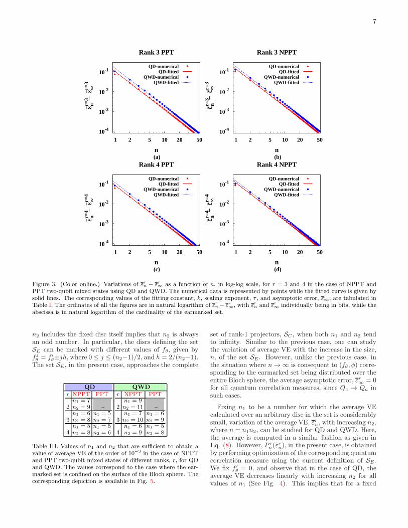
Figure 13. (Color online.) Variation of Dc and Da for ρa,as functions of the state parameter a, when measurement isperformed over the subsystem B. (Inset) Variation of VE, ε,as a function of a. The quantities Dc, Da, and ε are in bits,while a is dimensionless.

ment observable is Sx. Similar results are obtained in thecase of QWD and CQWD (Fig. 12(b)) where the max-imum VE occurs at a = 0.32. In both the cases (QDand QWD), the maximum VE is of the order of ∼ 10−1,which is much higher compared to the same in previousexamples.

An interesting observation comes from swapping thesubsystem over which the local measurement is performedsince the state ρa is asymmetric over an exchange of thesubsystems A and B. If one optimizes QD of ρa overa complete set of local measurements performed on theparty B instead of A, it is observed that the VE reducesdrastically in comparison to the same obtained when mea-surement is performed over the party A. The variation ofthe corresponding Dc and Da along with VE against thestate parameter a is given in Fig. 13. The VE attainsa non-zero value (from the zero value) at a = 0.6, whilea sudden change in the variation profile is observed ata = 0.665. This change is due to a transition of the opti-mal measurement observable from Sy to Sx at a = 0.665.Note that the maximum value of VE in the region a ≥ 0.6is ∼ 10−2, in contrast to the previous case. Note alsothat analytical expressions for CQD and CQWD can beobtained in a procedure similar as in the previous case.

Case 2

Let us take another example of a PPT BE state in C3⊗C3, given by [17]:

α =2

7|ψ〉〈ψ|+ α

7+ +

5− α

7−, (33)

0.34

0.36

0.38

0.4

0.42

0.44

0.46

0 1 2 3 4 5

QD

α

DcDa

(a)

0×100

2×10-3

4×10-3

6×10-3

8×10-3

1×10-2

0 1 2 3 4 5

ε

α

(a)

(b)

Figure 14. (Color online.) Variation of QD (a) and the corre-sponding VE (b) as functions of α in the case of the PPT BEstate α, given in Eq. (33). The quantities Dc, Da, and ε arein bits, while α is dimensionless.

where + = (|01〉〈01| + |12〉〈12| + |20〉〈20|)/3, − =

(|10〉〈10|+ |21〉〈21|+ |02〉〈02|)/3, |ψ〉 = 1√3

∑2i=0 |ii〉, and

0 ≤ α ≤ 5. The state is separable for 2 ≤ α ≤ 3, BE for3 < α ≤ 4 and 1 < α ≤ 2, while distillable for 4 < α ≤ 5and 0 < α ≤ 1 [17]. Fig. 14(a) depicts the variationof QD and CQD as functions of the state parameter αover its entire range. Note that the QD as well as theCQD remains constant over the range of α in which en-tanglement is distillable, whereas both of them attains aminimum at α = 2.5 in the separable region. In the BEregion, 1 < α ≤ 2, the value of QD as well as CQD re-mains constant up to α = 1.36, and then decreases forincreasing α in the region 1.36 ≤ α ≤ 2. Besides, in theBE region, 3 < α ≤ 4, the value of QD as well as CQDincreases with increasing α up to α = 3.64, and then be-comes constant. The corresponding ε is plotted againstα in Fig. 14(b). Note that the maximum VE is com-mitted in the separable region (of the order of ∼ 10−2),

17

whereas it is smaller (of the order of ∼ 10−3) in the BEregion. Clearly, the maximum VE is relatively higher inthe present case in comparison to the C2 ⊗ C4 BE state,ρb (Eq. (23)), but considerably lower when compared tothe C3 ⊗ C3 BE state, ρa (Eq. (32)). When QD is con-stant, the optimal measurement observable is Sz while itchanges to either Sx or Sy when value of QD increases ordecreases. Note that in the latter case, choice of Sx or Sy

as the optimal measurement observable are equivalent inthe context of optimizing QD. Analytic expression for Dc

can be obtained using the above analysis, as shown in theprevious cases.We conclude the discussion on the state α by pointing

out that the QWD of the state coincides with the QDsince α has maximally mixed marginals, i.e., the localdensity operator of each of the parties is proportional toidentity in C3 [10].

V. CONCLUDING REMARKS

To summarize, we have addressed the question whetherthe computational complexity of information theoreticmeasures of quantum correlations such as quantum dis-cord and quantum work deficit can be reduced by per-forming the optimization involved over a constrained sub-set of local projectors instead of the complete set. We haveconsidered four plausible constructions of such a restrictedset, and shown that the average absolute error, in the caseof two-qubit mixed states with different ranks, dies downfast with the increase in the size of the set. Quantitativeinvestigation of the reduction of error with the increasein the size of the restricted set has been performed witha comparative study between quantum discord and quan-tum work deficit, and the corresponding scaling exponentshave been estimated. We have also considered a general

two-qubit state up to local unitary transformation, andhave shown that the computation of measures like quan-tum discord and quantum work deficit can be made con-siderably easier by carefully choosing the restricted set ofprojectors. We have also pointed out that insight aboutconstructing the constrained set can be gathered from theprobability distribution of the optimizing parameters.

If a very special restricted set consisting of the projec-tion measurements corresponding to only the three Paulimatrices is considered, we have demonstrated that thestate space of a two-qubit system contains a large frac-tion of states for which exact minimizations of quantumdiscord and quantum work deficit are obtained only onthis set, resulting vanishing error. We have also pointedout that this feature can be utilized to obtain closed-formexpressions of quantum correlation measures up to smallerror for some special classes of states, which can be usedto study physical systems such as quantum spin mod-els. The usefulness of this methodology has been demon-strated in the finite size scaling analysis of the well-knowntransverse-field XY model at zero temperature, and forthe thermal state of a two-qubit XY model in an externalinhomogeneous transverse field. Moreover, we have foundthat the absolute error in the value of quantum correla-tion calculated using the constrained set in the case oftwo-qubit PPT as well as PPT BE states is low comparedto the NPPT states. The investigations show that thesemeasures can be obtained with high accuracy even whenrestrictions in the optimizations involved in their defini-tions are employed, thereby reducing the computationaldifficulties in their evaluation. Although we have inves-tigated only information theoretic measures, this studygives rise to a possibility to overcome challenges in thecomputation of other quantum correlation measures thatinvolve optimization over some set.

[1] R. Horodecki, P. Horodecki, M. Horodecki, and K.Horodecki, Rev. Mod. Phys. 81, 865 (2009).

[2] C. H. Bennett and S.J. Wiesner, Phys. Rev. Lett. 69, 2881(1992); C. H. Bennett, G. Brassard, C. Crepeau, R. Jozsa,A. Peres, and W. K. Wootters, Phys. Rev. Lett. 70, 1895(1993); R. Raussendorf and H. J. Briegel, Phys. Rev. Lett.86, 5188 (2001); P. Walther, K. J. Resch, T. Rudolph, E.Schenck, H. Weinfurter, V. Vedral, M. Aspelmeyer, andA. Zeilinger, Nature 434, 169 (2005); H. J. Briegel, D.Browne, W. Dur, R. Raussendorf, and M. van den Nest,Nat. Phys. 5, 19 (2009).

[3] J. M. Raimond, M. Brune, S. Haroche, Rev. Mod. Phys.73, 565 (2001); D. Leibfried, R. Blatt, C. Monroe, and D.Wineland, Rev. Mod. Phys. 75, 281 (2003); L. M. K. Van-dersypen, I.L Chuang, Rev. Mod. Phys. 76, 1037 (2005);K. Singer, U. Poschinger, M. Murphy, P. Ivanov, F. Ziesel,T. Calarco, F. Schmidt-Kaler, Rev. Mod. Phys. 82, 2609(2010); H. Haffner, C. F. Roose, R. Blatt, Phys. Rep. 469,155 (2008); L.-M. Duan, C. Monroe, Rev. Mod. Phys. 82,

1209 (2010); J.-W. Pan, Z.-B. Chen, C.-Y. Lu, H. Wein-

furter, A. Zeilinger, M. Zukowski, Rev. Mod. Phys. 84,777 (2012).

[4] C. H. Bennett, G. Brassard, S. Popescu, B. Schumacher, J.A. Smolin, and W. K. Wootters, Phys. Rev. Lett. 76, 722(1996); M. Horodecki, P. Horodecki, and R. Horodecki,Phys. Rev. Lett. 78, 574 (1997); M. Murao, M. B. Plenio,S. Popescu, V. Vedral, and P. L. Knight, Phys. Rev. A57, R4075 (1998); W. Dur, J. I. Cirac, and R. Tarrach,Phys. Rev. Lett. 83, 3562 (1999); M. Horodecki and P.Horodecki, Phys. Rev. A 59, 4206 (1999); W. Dur andJ. I. Cirac, Phys. Rev. A 61, 042314 (2000); W. Dur, J.I. Cirac, M. Lewenstein, and D. Bruß, Phys. Rev. A 61,062313 (2000); G. Alber, A. Delgado, N. Gisin, and I. Jex,J. Phys. A. 34, 8821 (2001); J. Dehaene, M. Van den Nest,B. D. Moor, and F. Vestraete, Phys. Rev. A 67, 022310(2003); W. Dur, H. Aschaur, and H. J. Briegel, Phys. Rev.Lett. 91, 107903 (2003); E. Hostens, J. Dehaene, and B.D. Moor, arXiv:quant-ph/0406017 (2004); K. G. H. Voll-

18

brecht and F. Vestraete, Phys. Rev. A 71, 062325 (2005);A. Miyake and H. J. Briegel, Phys. Rev. Lett. 95, 220501(2005); H. Aschaur, W. Dur, and H. J. Briegel, Phys. Rev.A 71, 012319 (2005); E. Hostens, J. Dehaene, and B. D.Moor, Phys. Rev. A 73, 042316 (2006); E. Hostens, J. De-haene, and B. D. Moor, Phys. Rev. A 74, 062318 (2006);A. Kay, J. K. Pachos, W. Dur, and H. J. Briegel, New.J. Phys. 8, 147 (2006); C. Kruszynska, A. Miyake, H. J.Briegel, and W. Dur, Phys. Rev. A 74, 052316 (2006); S.Glancy, E. Knill, and H. M. Vasconcelos, Phys. Rev. A74, 032319 (2006).

[5] C. H. Bennett, D. P. DiVincenzo, C. A. Fuchs, T. Mor,E. Rains, P. W. Shor, J. A. Smolin, and W. K. Wootters,Phys. Rev. A 59, 1070 (1999); C. H. Bennett, D.P. DiVin-cenzo, T. Mor, P.W. Shor, J.A. Smolin, and B.M. Terhal,Phys. Rev. Lett. 82, 5385 (1999); D. P. DiVincenzo, T.Mor, P. W. Shor, J. A. Smolin, and B. M. Terhal Com-mun. Math. Phys. 238, 379 (2003).

[6] A. Peres and W.K. Wootters, Phys. Rev. Lett. 66, 1119(1991); J. Walgate, A.J. Short, L. Hardy, and V. Ve-dral,ibid. 85, 4972 (2000); S. Virmani, M.F. Sacchi, M.B.Plenio, and D. Markham, Phys. Lett. A 288, 62 (2001);Y.-X. Chen and D. Yang, Phys. Rev. A 64, 064303(2001);ibid. 65, 022320 (2002); J. Walgate and L. Hardy,Phys. Rev. Lett. 89, 147901 (2002); M. Horodecki, A.Sen(De), U. Sen, and K. Horodecki, ibid. 90, 047902(2003); W. K. Wootters, Int. J. Quantum Inf. 4, 219(2006).

[7] E. Knill and R. Laflamme, Phys. Rev. Lett. 81, 5672(1998); A. Datta, A. Shaji, and C. M. Caves, Phys. Rev.Lett. 100, 050502 (2008); B. P. Lanyon, M. Barbieri, M. P.Almeida, and A. G. White, Phys. Rev. Lett. 101, 200501(2008).

[8] B. Dakic, V. Vedral, and C. Brukner, Phys. Rev. Lett.105, 190502 (2010).

[9] L. Henderson and V. Vedral, J. Phys. A 34, 6899 (2001);H. Olivier and W. H. Zurek, Phys. Rev. Lett. 88, 017901(2001); W. H. Zurek, Rev. Mod. Phys. 75, 715 (2003).

[10] J. Oppenheim, M. Horodecki, P. Horodecki and R.Horodecki, Phys. Rev. Lett. 89, 180402 (2002); M.Horodecki, K. Horodecki, P. Horodecki, R. Horodecki, J.Oppenheim, A. Sen(De), and U. Sen, Phys. Rev. Lett.90, 100402 (2003); I. Devetak, Phys. Rev. A 71, 062303(2005); M. Horodecki, P. Horodecki, R. Horodecki, J. Op-penheim, A. Sen(De), U. Sen, and B. Synak-Radtke, Phys.Rev. A 71, 062307 (2005).

[11] L. C. Celeri, J. Maziero, and R. M. Serra, Int. J. Quant.Inf. 9, 1837 (2011), and the references therein.

[12] K. Modi, A. Brodutch, H. Cable, T. Paterek, and V. Ve-dral, Rev. Mod. Phys. 84, 1655 (2012), and the referencestherein.

[13] M. Koashi, and A. Winter, Phys. Rev. A 69, 022309(2004); F. F. Fanchini, M. F. Cornelio, M. C. de Oliveira,and A. O. Caldeira, Phys. Rev. A 84, 012313 (2011);S. Yu, C. Zhang, Q. Chen, and C. Oh, arXiv:1102.1301[quant-ph] (2011); C. Zhang, S. Yu, Q. Chen, and C. Oh,Phys. Rev. A 84, 052112 (2011); L.-X. Cen, X.-Q. Li, J.Shao, and Y. Yan, Phys. Rev. A 83, 054101 (2011); F.Galve, G. Giorgi, and R. Zambrini, Europhys. Lett. 96,40005 (2011); A. Al-Qasimi and D. F. V. James, Phys.Rev. A 83, 032101 (2011); T. K. Chuan, J. Maillard, K.Modi, T. Paterek, M. Paternostro, and M. Piani, Phys.Rev. Lett. 109, 070501 (2012); F. Lastra, C. Lopez, L.

Roa, and J. Retamal, Phys. Rev. A 85, 022320 (2012); F.F. Fanchini, L. K. Castelano, M. F. Cornelio, and M. C.de Oliveira, New J. Phys. 14, 013027 (2012); Z. Xi, X.-M.Lu, X. Wang, and Y. Li, Phys. Rev. A 85, 032109 (2012).

[14] A. Streltsov, H. Kampermann, and D. Bruß, Phys. Rev.Lett. 106, 160401 (2011); M. Piani, S. Gharibian, G.Adesso, J. Calsamiglia, P. Horodecki, and A. Winter,Phys. Rev. Lett. 106, 220403 (2011); M. F. Cornelio, M.C. de Oliveira, and F. F. Fanchini, Phys. Rev. Lett. 107,020502 (2011); X. Q. Yan, G. H. Liu, and J. Chee, Phys.Rev. A 87, 022340 (2013).

[15] P. Horodecki, Phys. Lett. A 232, 333 (1997).[16] M. Horodecki, P. Horodecki, and R. Horodecki, Phys. Rev.

Lett. 80, 5239 (1998).[17] P. Horodecki, M. Horodecki, and R. Horodecki, Phys. Rev.

Lett. 82, 1056, (1999).[18] D. Bruss, A. Peres, Phys. Rev. A. 61, 030301(R) (2000).[19] W. Dur and J. I. Cirac, Phys. Rev. A 62, 022302 (2000);

P. Horodecki, J. A. Smolin, B. M. Terhal, and A. V. Thap-liyal, Theor. Comput. Sc. 292, 589 (2003); J. Lavoie, R.Kaltenbaek, M. Piani, and K. J. Resch, Nature Physics6, 827 (2010); J. Lavoie, R. Kaltenbaek, M. Piani, andK. J. Resch, Phys. Rev. Lett. 105, 130501 (2010); J.DiGuglielmo, A. Samblowski, B. Hage, C. Pineda, J. Eis-ert, and R. Schnabel, Phys. Rev. Lett. 107, 240503 (2011);E. Amselem, M. Sadiq, and M. Bourennane, Scientific Re-ports 3, 1966 (2013).

[20] T. Moroder, O. Gittsovich, M. Huber, and O. Guhne,Phys. Rev. Lett. 113, 050404 (2014).

[21] D. P. DiVincenzo, P. W. Shor, J. A. Smolin, B. M. Terhal,and A. V. Thapliyal, Phys. Rev. A 61, 062312 (2000); B.Kraus, M. Lewenstein, and J. I. Cirac, Phys. Rev. A 65,042327 (2002); J. Watrous, Phys. Rev. Lett. 93, 010502(2004).

[22] S. Luo, Phys. Rev. A 77, 042303 (2008).[23] M. Ali, A. R. P. Rau, and G. Alber, Phys. Rev. A 81,

042105 (2010); ibid. 82, 069902(E), (2010); X.-M. Lu, J.Ma, Z. Xi, and X. Wang, Phys. Rev. A 83, 012327 (2011);D. Girolami and G. Adesso, Phys. Rev. A 83, 052108(2011); Q. Chen, C. Zhang, S. Yu, X. X. Yi, and C. H.Oh, Phys. Rev. A 84, 042313 (2011).

[24] M. Ali, J. Phys. A: Math. Theor. 43, 495303 (2010); S.Vinjanampathy and A. R. P. Rau, J. Phys. A: Math.Theor. 45, 095303 (2012); B. Ye, Y. Liu, J. Chen, X.Liu, and Z. Zhang, Quant. Inf. Process. 12, 2355 (2013).

[25] Y. Huang, New. J. Phys. 16 (3), 033027 (2014).[26] M. A. Yurishchev, Phys. Rev. B 84, 024418 (2011); R.

Auccaise, J. Maziero, L. C. C eleri, D. O. Soares-Pinto,E. R. deAzevedo, T. J. Bonagamba, R. S. Sarthour, I. S.Oliveira, and R. M. Serra, Phys. Rev. Lett. 107, 070501(2011); G. Passante, O. Moussa, D. A. Trottier, and R.Laflamme, Phys. Rev. A 84, 044302 (2011); L. S. Madsen,A. Berni, M. Lassen, and U. L. Andersen, Phys. Rev. Lett.109, 030402 (2012). M. Gu, H. M. Chrzanowski, S. M.Assad, T. Symul, K. Modi, T. C. Ralph, V. Vedral, andP. K. Lam, Nature Phys. 8, 671 (2012); R. Blandino,M. G. Genoni, J. Etesse, M. Barbieri, M. G. A. Paris,P. Grangier, and R. Tualle-Brouri, Phys. Rev. Lett. 109,180402 (2012); U. Vogl, R. T. Glasser, Q. Glorieux, J. B.Clark, N. V. Corzo, and P. D. Lett, Phys. Rev. A 87,010101(R) (2013); C. Benedetti, A. P. Shurupov, M. G.A. Paris, G. Brida, and M. Genovese, Phys. Rev. A 87,052136 (2013).

19

[27] Y. Huang, Phys. Rev. A 88, 014302 (2013); M. Namkung,J. Chang, J. Shin, and Y. Kwon, Int. J. Theor. Phys. 54,3340 (2015).

[28] F. F. Fanchini, T. Werlang, C. A. Brasil, L. G. E. Arruda,and A. O. Caldeira, Phys. Rev. A 81, 052107 (2010); B.Li, Z. -X. Wang, and S. -M. Fei, Phys. Rev. A 83, 022321(2011).

[29] T. Chanda, A. K. Pal, A. Biswas, A. Sen(De), and U. Sen,Phys. Rev. A 91, 062119 (2015).

[30] C. W. Helstrom, Quantum Detection and Estimation The-ory (Academic Press, New York, 1976); A.S. Holevo, Sta-tistical Structure of Quantum Theory, Lect. Not. Phys.61 (Springer, Berlin, 2001); C. W. Helstrom, Phys. Lett.A 25, 1012 (1967); H. P. Yuen, M. Lax, IEEE Trans.Inf. Th. 19, 740 (1973); C. W. Helstrom, R. S. Kennedy,IEEE Trans. Inf. Th. 20, 16 (1974); S. Braunstein and C.Caves, Phys. Rev. Lett. 72, 3439 (1994); S. Braunstein,C. Caves, and G. Milburn, Ann. Phys. 247, 135 (1996);M. G. A. Paris, Int. J. Quant. Inform., 07, 125 (2009),and the references therein.

[31] A. Peres, Phys. Rev. Lett. 77, 1413 (1996); M. Horodecki,P. Horodecki, and R. Horodecki, Phys. Lett. A 223, 1(1996).

[32] T. Eu and J. H. Eberly, Quant. Inform. Comput. 7, 459(2007).

[33] E. Lieb, T. Schultz, and D. Mattis, Ann. Phys. 16, 407(1961); E. Barouch, B.M. McCoy, and M. Dresden, Phys.Rev. 2, 1075 (1970); P. Pfeuty, Ann. Phys. 57, 79 (1970);E. Barouch and B.M. McCoy, Phys. Rev. 3, 786 (1971).

[34] N. J. Cerf, C. Adami, Phys. Rev. Lett. 79, 5194 (1997);B. Groisman, S. Popescu, and A. Winter, Phys. Rev. A72, 032317 (2005).

[35] S. Luo and S. Fu, Phys. Rev. A 82, 034302 (2010); X.-M. Lu, Z. -J. Xi, Z. Sun, and X. Wang, Quant. Info.Comput., 10, 0994 (2010); T. Debarba, T. O. Maciel, andR. O. Vianna, Phys. Rev. A 86, 024302 (2012); J. -S.Jin, F. -Y Zhang, C.-S. Yu, and H. -S. Song, J. Phys. A:Math. Theor. 45, 115308 (2012); J. D. Montealegre, F. M.Paula, A. Saguia, and M. S. Sarandy, Phys. Rev. A 87,042115 (2013); D. Spehner and M. Orszag, New J. Phys.15, 103001 (2013); D. Spehner and M. Orszag, J. Phys.A: Math. Theor. 47, 035302 (2014).

[36] D. Girolami and G. Adesso, Phys. Rev. A 84, 052110(2011).

[37] B. Dakic, Y. O. Lipp, X. Ma, M. Ringbauer, S.Kropatschek, S. Barz, T. Paterek, V. Vedral, A. Zeilinger,Caslav Brukner, and P. Walther, Nature Phys. 8, 666(2012).

[38] M. Piani, Phys. Rev. A 86, 034101 (2012).[39] F. M. Paula, Thiago R. de Oliveira, and M. S. Sarandy,

Phys. Rev. A 87, 064101 (2013).[40] F. Ciccarello, T. Tufarelli, and V Giovannetti, New J.

Phys. 16, 013038 (2014).[41] L. Roa, J. C. Retamal, and M. Alid-Vaccarezza, Phys.

Rev. Lett. 107, 080401 (2011); V. Madhok and A. Datta,Phys. Rev. A 83, 032323 (2011); V. Madhok and A. Datta,Int. J. Mod. Phys. B 27, 1345041 (2013).

[42] A two-qubit rank-2 state can be written as ρ = p|ψ〉〈ψ|+(1 − p)|φ〉〈φ|, where 0 ≤ p ≤ 1, and |ψ〉 and |φ〉 are mu-tually orthogonal. The state |ψ〉, in Schmidt decomposedform, can be written as |ψ〉 = α|00〉 + β|11〉, where α,β, are real and α2 + β2 = 1. The partial transposition,ρT , of ρ will always have a negative eigenvalue given byλ = −|2pαβ−1|. The state is PPT only when λ = 0, whichcorresponds to a line in the state space of all rank-2 states.Therefore, the PPT states in the space of all rank-2 statesform a set of measure zero.

[43] K. Zyczkowski, P. Horodecki, A. Sanpera, and M. Lewen-stein, Phys. Rev. A 58, 883 (1998), and references thereto.

[44] C. N. Yang and C. P. Yang, Phys. Rev. 150, 321 (1966); C.N. Yang and C. P. Yang, Phys. Rev. 150, 327 (1966); A.Langari, Phys. Rev. B 58, 14467 (1998); D. V. Dmitriev,V. Y. Krivnov, A. A. Ovchinnikov, and A. Langari, J.Exp. Theor. Phys. 95, 538 (2002); S Mahdavifar, J. Phys.:Condens. Matter 19 406222 (2007).

[45] L. Amico, R. Fazio, A. Osterloh, and V. Vedral, Rev. Mod.Phys. 80, 517 (2008); J. I. Latorre, and A. Rierra, J. Phys.A 42, 504002 (2009); J. Eisert, M. Cramer, and M. B.Plenio, Rev. Mod. Phys. 82, 277, (2010).

[46] A. Osterloh, L. Amico, G. Falci, and R. Fazio, Nature416, 608 (2002); T. Osborne, and M. Nielsen, Phys. Rev.A 66, 032110 (2002); G. Vidal, J. Latorre, E. Rico, andA. Kitaev, Phys.Rev. Lett. 90, 227902 (2003).

[47] R. Dillenschneider, Phys. Rev. B 78, 224413 (2008); M.S. Sarandy, Phys. Rev. A 80, 022108 (2009).

[48] M. Schechter and P. C. E. Stamp, Phys. Rev. B 78, 054438(2008).

[49] X. -L. Deng, D. Porras, and J. I. Cirac, Phys. Rev. A 72,063407 (2005).

[50] M. Lewenstein, A. Sanpera, V. Ahufinger, B. Damski,A.Sen(De), and U. Sen, Adv. Phys. 56, 243 (2007).

[51] R. Islam, E. E. Edwards, K. Kim, S. Korenblit, C. Noh,H. Carmichael, G.-D. Lin, L.-M. Duan, C.-C. JosephWang, J. K. Freericks, and C. Monroe, Nature Commun.2, 377 (2011); J. Struck, M. Weinberg, C. Olschlger, P.Windpassinger, J. Simonet, K. Sengstock, R. Hoppner, P.Hauke, A. Eckardt, M. Lewenstein, and L. Mathey, Na-ture Physics 9, 738 (2013), and references therein.

[52] B. K. Chakrabarti, A. Dutta, and P. Sen, QuantumIsing Phases and Transitions in Transverse Ising Mod-els (Springer, Heidelberg, 1996); S. Sachdev, QuantumPhase Transitions (Cambridge University Press, Cam-bridge, 2011); S. Suzuki, J. -I. Inou, B. K. Chakrabarti,Quantum Ising Phases and Transitions in Transverse IsingModels (Springer, Heidelberg, 2013).