REDUCING THE OVERFITTING OF ADABOOST BY …web.engr.oregonstate.edu/~sinisa/research/publications/IJPRAI06.pdf · November 10, 2006 14:11 WSPC/115-IJPRAI SPI-J068 00513 Reducing Overﬁtting

November 10, 2006 14:11 WSPC/115-IJPRAI SPI-J068 00513

International Journal of Pattern Recognitionand Artificial IntelligenceVol. 20, No. 7 (2006) 1093–1116c© World Scientific Publishing Company

REDUCING THE OVERFITTING OF ADABOOST BYCONTROLLING ITS DATA DISTRIBUTION SKEWNESS

YIJUN SUN∗,†,‡, SINISA TODOROVIC§ and JIAN LI‡

†Interdisciplinary Center for Biotechnology Research‡Department of Electrical and Computer Engineering, University of Florida

Gainesville, FL 32611-6130, USA

§3021 Beckman Institute of Advanced Science and TechnologyUniversity of Illinois at Urbana-Champaign

405 N. Mathews Ave., Urbana, IL 61801, USA∗[email protected]

AdaBoost rarely suffers from overfitting problems in low noise data cases. However,recent studies with highly noisy patterns have clearly shown that overfitting canoccur. A natural strategy to alleviate the problem is to penalize the data distri-bution skewness in the learning process to prevent several hardest examples fromspoiling decision boundaries. In this paper, we pursue such a penalty scheme in themathematical programming setting, which allows us to define a suitable classifier softmargin. By using two smooth convex penalty functions, based on Kullback–Leiblerdivergence (KL) and l2 norm, we derive two new regularized AdaBoost algorithms,referred to as AdaBoostKL and AdaBoostNorm2, respectively. We prove that our algo-rithms perform stage-wise gradient descent on a cost function, defined in the domainof their associated soft margins. We demonstrate the effectiveness of the proposed algo-rithms through experiments over a wide variety of data sets. Compared with otherregularized AdaBoost algorithms, our methods achieve at least the same or betterperformance.

Keywords: Adaptive boosting (AdaBoost); minimax problem; margin; soft margin;regularization.

1. Introduction

The adaptive boosting (AdaBoost) algorithm is considered one of the most impor-tant developments in the classification methodology in recent years. It has been usedwith great success in many applications.8,12,21 In the low noise regime, empiricalevidence indicates that AdaBoost rarely suffers from overfitting problems. One lead-ing explanation to understand this phenomenon is contemplated to be the marginconcept.20 It has been empirically observed that AdaBoost can effectively increase

∗Author for correspondence.

1093


1094 Y. Sun, S. Todorovic & J. Li

the margin, and a large margin, in turn, is usually conducive to good generaliza-tion, in the sense that if a large margin can be achieved with respect to given data,an upper bound on the generalization error is small.22 Recent studies with highlynoisy patterns,5,10,14,16 however, have shown that overfitting may occur. Therefore,in the light of AdaBoost’s increasing popularity, it is important to examine theoverfitting phenomenon, and to seek effective solutions, which would enhance theperformance of AdaBoost in noisy settings.

It has been reported that the main reason for poor classification results ofAdaBoost in the high-noise regime is that the algorithm produces a skewed datadistribution, by assigning too much weight onto a few hard-to-learn examples.5

Therefore, one natural strategy is to introduce a regularization term into the algo-rithm, which would control the data distribution skewness. Based on this principle,one of the earliest proposed algorithms is AdaBoostReg.16 It is a heuristic algo-rithm based on an intuitive idea of controlling the tradeoff between the margin andthe sample influences to achieve a soft margin. In comparison with other availableregularized boosting algorithms, AdaBoostReg yields among the best generalizationresults on noisy data. However, since the regularization is introduced on the algo-rithm level, it is difficult to analyze its underlying optimization scheme, and theultimate goal of the algorithm is obscure.12,14

Since it is not straightforward to include a regularization term into AdaBoost,a potentially better way to design new regularized boosting algorithms may beto exploit the close relationship between AdaBoost and the well-known minimaxproblem. As an advantage of this approach, some of the well-studied mathemat-ical programming techniques can be directly utilized. One typical representativeof this strategy is LPreg-AdaBoost, which constitutes the underlying optimizationscheme of ν-Arc,17 and C-Barrier algorithms.14 In LPreg-AdaBoost, slack variablesare introduced into an optimization problem in the primal domain, similar to Sup-port Vector Machine (SVM) in the nonseparable data case. In the dual domain, weshow this algorithm is equivalent to constraining the data distribution to a box. Assuch, this algorithm can be understood as a penalty scheme with a zero penaltywithin the box and infinity outside the box. In this sense, the scheme is somewhatheuristic, and may be too restrictive.

In this paper, we instead consider controlling the skewness of data distributionsby adding a convex penalty function to the objective function of the minimaxproblem. By means of the generalized minimax theorem, we show that the penaltyscheme can be pursued equivalently in the dual domain, wherein we specify thegeneral framework of the proposed regularization. This general framework gives riseto a range of regularized boosting algorithms, differing in a particular specificationof the penalty function. For example, we show that LPreg-AdaBoost can be derivedfrom the outlined framework if the penalty is defined as a hard-limited function,which is a novel interpretation of the algorithm. We study two penalty functionsthat are based on the Kullback–Leibler (KL) divergence, and lp norm. From theminimax optimization problem, where these two penalty functions are introduced,


Reducing Overfitting of AdaBoost by Controlling Distribution Skewness 1095

we derive the soft margin, and two novel regularized AdaBoost algorithms, referredto as AdaBoostKL and AdaBoostNorm2. These two algorithms can be viewed asan extension of AdaBoostReg; the main difference is in specification of the softmargin. We believe that the soft margin in our methods is more reasonable thanthat in AdaBoostReg with respect to two criteria. First, we prove that our algorithmsperform the stage-wise gradient descent of a cost function, defined in the domainof the soft margin, whereas AdaBoostReg does not have such property. Second,AdaBoostKL and AdaBoostNorm2 outperform AdaBoostReg. To demonstrate theeffectiveness of our algorithms, we report experiments on a wide variety of artificialand real-world data sets, where we compare the performance of our algorithms withthat of AdaBoostReg, ν-Arc, C-Barrier and SVM. We record that the classificationresults of AdaBoostKL and AdaBoostNorm2 are among the best.

The rest of the paper is organized as follows. First, in Sec. 2, we present a briefreview of AdaBoost. In Sec. 3, we propose two new algorithms, namely AdaBoostKL

and AdaBoostNorm2. In Sec. 4, we report experiments on a wide variety of data sets,where we compare the performance of our algorithms with that of AdaBoostReg,ν-Arc, C-Barrier and SVM. We conclude the paper in Sec. 5.

Throughout, a vector is denoted as a boldface low-case letter, and a matrix, asa boldface upper-case letter. The ijth entry of a matrix Z is written as zij . z.i andzj. are the ith column and jth row of Z, respectively. The unnormalized vector ofa is denoted as a, that is, a = a/‖a‖1, where ‖ · ‖p is the p-norm.

2. AdaBoost

In this section, we briefly review AdaBoost, as well as its interpretation as a func-tional gradient-descent procedure. For a thorough description, the interested readeris referred to a good tutorial paper,12 and references therein.

Suppose we are given a training data set D = {(xn, yn)}Nn=1 ∈ X×Y, where X is

a pattern space and Y = {±1} is a label space. Given a class of hypothesis functionsH = {h(x) : x → ±1}, called weak learners or base learners, we are interested infinding an ensemble function F (x) =

∑t αtht(x), or f(x) =

∑t αtht(x), such

that a certain cost function is minimized, where αt � αt/∑

t αt. Both the vectorof combination coefficients α and hypothesis functions ht(x) are learned in thelearning process. Several ensemble methods have been developed for this purpose,among which AdaBoost is the most popular.8 The pseudo code of AdaBoost ispresented in Fig. 1.

AdaBoost can be viewed as an algorithm performing stage-wise gradient descentof a cost function of margins G defined as

G � 1N

N∑n=1

exp(−ynF (xn)),

=1N

N∑n=1

exp

(−ρ(xn)

∑t

αt

), (4)



AdaBoostInitialization: D = {(xn, yn)}N

n=1, maximum number of iteration steps T , d(1)n =

1/N , n = 1, . . . , N

for t = 1 : T

1. Train the weak learner with respect to distribution d(t) andget hypothesisht(x) : x → {±1}.2. Calculate the weighted training error εt of ht:

εt =N∑

n=1

d(t)n I(yn �= ht(xn)) , (1)

where I(·) is the indicator function.3. Compute the combination coefficient:

αt =12

ln(

1 − εt

εt

), (2)

4. Update weights for n = 1, . . . , N :

d(t+1)n = d(t)

n exp (−αtynht(xn)) /Ct (3)

where Ct is the normalization constant,such that

∑Nn=1 d

(t+1)n = 1.

endOutput : F (x) =

∑Tt=1 αtht(x)

Fig. 1. Pseudo code of AdaBoost.

where ρ(xn) � ynf(xn) denotes the margin of sample xn with respect to f(xn). Atthe tth iteration, the negative functional derivative of G at Ft−1 is given by

−∇G(Ft−1)(x) =

0, if x �= xn

1N

yn exp(−ynFt−1(xn)), if x = xn, n = 1, . . . , N.(5)

Equation (5) represents the direction, in which the cost function most rapidlydecreases. Since the choice of the new ht is constrained to H, it may not be possibleto choose ht = −∇G(Ft−1)(x).11 Instead, the search for ht is conducted such thatthe inner product given by

〈−∇G, ht〉 =1N

N∑n=1

exp(−ynFt−1(xn))ynht(xn) ,

=∑N

i=1 exp(−ynFt−1(xn))N

N∑n=1

exp(−ynFt−1(xn))∑Ni=1 exp(−yiFt−1(xi))

ynht(xn), (6)



is maximized.9 By unravelling Eq. (3) in Fig. 1, we get

d(t)n = d(t−1)

n exp(−αt−1ynht−1(xn))/Ct−1 =exp(−ynFt−1(xn))∑Ni=1 exp(−yiFt−1(xi))

. (7)

From Eqs. (6) and (7), it immediately follows that ht(x) is chosen to minimize theweighted error in Eq. (1). After ht(x) is selected, coefficient αt can be found by aline search to minimize the intermediate cost function:

G(t) =1N

N∑n=1

exp

(−yn

(t−1∑i=1

αihi(xn) + αtht(xn)

)). (8)

In the binary classification case, i.e. H = {h(x) : x → ±1}, αt can be computed ana-lytically as a solution to ∂Gt/∂αt = 0, which is equal to the closed form in Eq. (2).

It has been empirically observed that AdaBoost can effectively increase themargin.20 For this reason, since the invention of AdaBoost, it has been conjecturedthat AdaBoost, in the limit (i.e. t → ∞), solves the following linear programming(LP) problem:

max ρ,

s.t. ρ(xn) ≥ ρ, n = 1, . . . , N,(9)

where the margin is directly maximized. In the recent paper, however, the equiva-lence of the two algorithms has been proven not to hold always.18 Nevertheless, thesetwo algorithms are closely connected in the sense that both algorithms try to max-imize the margin. This observation motivates researchers to design new ensembleclassifiers either directly in the mathematical optimization setting,4,10 or by borrow-ing ideas from the optimization setting, and introducing them in boosting.14,16,17

Thereby, some of the well-studied optimization techniques can be utilized as novelboosting techniques.

3. Regularized AdaBoost

We begin the derivation of our regularization scheme by investigating the mini-max problem. The connection between the well-known minimax problem,23 andAdaBoost was first noted by Breiman,1 and Freund and Schapire.7 They deter-mined the maximum achievable margin, given a hypothesis class, by exploiting theduality relationships in linear programming. For the time being, we assume that thecardinality of the set of hypothesis functions, H, is finite and equal to T . We definea gain matrix, Z, where znt = ynht(xn) is the margin of sample xn with respectto the tth hypothesis function ht. Let us, now, examine the following minimaxoptimization problem:

maxα∈ΓT

mind∈ΓN

dTZα (10)

where ΓT is the distribution simplex defined as ΓT = {α : α ∈ RT ,∑T

t=1 αt =1, α ≥ 0}. The optimization scheme in Eq. (10) can be interpreted as finding a set



of combination coefficients α, such that the performance of the ensemble classifierin the worst case is optimized. It is straightforward to show that this optimizationscheme leads to the maximum margin scheme in Eq. (9).

Generally speaking, a large margin is usually conducive to good generalization;however, for noisy data, where the data samples are highly overlapped and/or afew samples are mislabeled, the maximum margin scheme can be easily misled byoutliers, yielding a classifier with suboptimal performance. Note that in Eq. (10), theminimization takes place over the entire probability space of the data distribution,which is not sufficiently restrictive. A natural strategy, therefore, is to constrain thedata distribution, or add a penalty term to the cost function to control the skewnessof the data distribution. Thereby, the algorithm will not be allowed to waste all ofits resources dealing with a few hard-to-learn samples. Below, we present threeregularized AdaBoost algorithms that fall into this framework.

3.1. LPreg-AdaBoost

By constraining the distribution to a box 0 ≤ d ≤ c, we obtain the followingoptimization problem:

maxα∈ΓT

min{d∈ΓN ,d≤c}

dTZα, (11)

where c is a constant vector, and usually takes a form of c = C1 with C beinga predefined parameter, and 1 ∈ RN being a vector of all ones. The optimizationscheme in Eq. (11) can be understood as finding a set of combination coefficients α,such that the classification performance, in the worst case, within the distributionbox, is maximized. The LP equivalent to Eq. (11) is

max(ρ,λ,α)

ρ −N∑

n=1

cnλn,

subject toT∑

t=1

αtznt ≥ ρ − λn, n = 1, . . . , N,

λn ≥ 0, n = 1, . . . , N, α ∈ ΓT .

(12)

LPreg-AdaBoost is a special case of Eq. (12) obtained by setting c1 = c2 = · · · =cN = C.16 A similar scheme is also used in Support Vector Machine for nonseparabledata cases.2 The optimization scheme in Eq. (12) introduces a nonnegative slackvariable λn into the optimization problem to achieve the soft margin, ρs(xn), ofpattern xn, defined as

ρs(xn) = ρ(xn) + λn. (13)

The relaxation of the hard margin allows some patterns to have a smaller marginthan ρ. Consequently, the algorithm does not classify all of the patterns accordingto their associated class labels.



The dual of Eq. (12) is given by

min(γ,d) γ,

subject toN∑

n=1

dnznt ≤ γ, t = 1, . . . , T,

d ≤ c,d ∈ ΓN .

(14)

By working directly in the dual domain, we lose the clarity of pursuing regulariza-tion through the margin concept. Yet, the dual domain proves advantageous, sincethe primal domain is not suitable for specifying the soft margin, except in the casedefined in Eq. (13).

For convenience, we reformulate Eq. (11) as

maxα∈ΓT

mind∈ΓN

dTZα + β(‖d‖∞), (15)

where ‖ · ‖p is the p-norm, and β(P ) is a function defined by

β(P ) =

{0, if P ≤ C,

∞, if P > C.(16)

Note that the box defined by {d : ‖d‖∞ ≤ C,d ∈ ΓN} is centered at the distributioncenter d0 = [1/N, . . . , 1/N ]. Also, the parameter C reflects to some extent thedistribution skewness between the box boundary and d0. Equation (15) indicatesthat LPreg-AdaBoost is a penalty scheme with a zero penalty within the box, andinfinity, outside the box. In this sense, this scheme is somewhat heuristic and maybe too restrictive.

With respect to the implementation of LPreg-AdaBoost, we note that in practicethe cardinality of H can be infinite. Consequently, the gain matrix Z may not existin an explicit form. As a result, the linear programming cannot be implementeddirectly. To overcome the problem, several algorithms have been proposed. Twotypical examples are ν-Arc,17 and C-Barrier algorithms.14

In the following sections, we use |H| to denote the cardinality of the hypothesisfunction set, and reserve T as the number of iteration steps in AdaBoost.

3.2. AdaBoostKL

Motivated by Eq. (15), one plausible strategy to control the skewness of the datadistribution is to add a penalty term, P (d), to the cost function in Eq. (10). Thepenalty can be defined as a function of the distance between query distributions dand distribution center d0. This leads to the following optimization problem:

maxα∈Γ|H|

mind∈ΓN

dTZα + βP (d), (17)



where β > 0 is a predefined parameter controlling the penalty strength. With amild assumption that P (d) is a convex function of d, it can be shown that Eq. (17)is equivalent to (Generalized Minimax Theorem6):

min(γ,d∈ΓN) γ + βP (d),

subject toN∑

n=1

dnznj ≤ γ, j = 1, . . . , |H|.(18)

We refer to the formulation in Eq. (18) as regularized scheme in the dual domain.One commonly used distance metric for two discrete distributions is the

Kullback–Leibler (KL) divergence.3 In our case, we have

KL(d,d0) =N∑

n=1

dn lndn

1/N. (19)

KL(d,d0) is convex over the region d > 0, because its Hessian matrix is positivedefinite.

By substituting Eq. (19) into Eq. (18), we derive

min(γ,d∈ΓN) γ + β

N∑n=1

dn lndn

1/N,

subject toN∑

n=1

dnznj ≤ γ, j = 1, . . . , |H|,(20)

which can be reformulated as

min(γ,d∈ΓN) γ,

subject toN∑

n=1

dnznj + βN∑

n=1

dn lndn

1/N≤ γ, j = 1, · · · , |H|. (21)

The above optimization problem is illustrated in Fig. 4(a) (|H| = 2). To facilitatethe following discussions, we introduce the following auxiliary terms:

sj(d) =N∑

n=1

dnznj + β

N∑n=1

dn lndn

1/N, (22)

s(d) = max1≤j≤|H|

sj(d). (23)

Note that s(d) is also a convex function.Suppose now we are given a set of query distributions {d(t)}T

t=1. For each querydistribution d(t), we can define a supporting hyperplane to the epigraph of s(d),given by

γ = s(d(t)) + ∂s(d(t))(d − d(t)), (24)



Due to the convexity of s(d), a supporting hyperplane gives an underestimate of s.More precisely, Eq. (24) can be written as

γ = max1≤j≤|H|

sj(d(t)) + ∂s(d(t))(d − d(t)),

= zT.td

(t) + β

N∑n=1

d(t)n ln

d(t)n

1/N+

z.t + β

ln d

(t)1

1/N + 1...

ln d(t)N

1/N + 1

T

(d − d(t)),

=(z.t + β ln

d(t)

1/N

)T

d, (25)

where

z.t = [y1ht(x1), . . . , yNht(xN )]T, (26)

and

ht = argmaxh∈H

N∑n=1

d(t)n h(xn)yn. (27)

Let us, now, define:

Z = Z + β

[ln

d(1)

1/N, . . . , ln

d(T )

1/N

], (28)

whose tth column reads z.t = z.t + β ln d(t)

1/N , where z.t is given by Eq. (26). Note

that Z can be interpreted as a new gain matrix. This means that adding a penaltyfunction to Eq. (10) results in a modification of the gain matrix that encodes thedistribution information into the hypothesis decisions. By using Eq. (28), the opti-mization problem in Eq. (21) can be approximated as

min(γ,d∈ΓN) γ,

subject to zT.td ≤ γ, t = 1, . . . , T.

(29)

Equation (29) represents a linear programming problem that is much easier to dealwith than the original one in Eq. (21). However, this is only a linear approximationthat becomes better as more constraints are added. The above linear approximationprocess is illustrated in Fig. 4(b).

The only remaining problem to be considered is the generation of the querydistributions. The distributions can be obtained by using a standard techniquecalled column generation.13 However, there are several drawbacks associated withthe column generation approach. Usually, it exhibits slow convergence due to thedegeneracy of Eq. (29). Moreover, a highly efficient LP solver is needed to compute



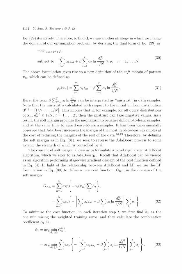
Eq. (29) iteratively. Therefore, to find d, we use another strategy in which we changethe domain of our optimization problem, by deriving the dual form of Eq. (29) as

max(ρ,α∈ΓT ) ρ,

subject toT∑

t=1

αtznt + β

T∑t=1

αt lnd(t)n

1/N≥ ρ, n = 1, . . . , N.

(30)

The above formulation gives rise to a new definition of the soft margin of patternxn, which can be defined as

ρs(xn) =T∑

t=1

αtznt + β

T∑t=1

αt lnd(t)n

1/N. (31)

Here, the term β∑T

t=1 αt ln d(t)n

1/N can be interpreted as “mistrust” in data samples.Note that the mistrust is calculated with respect to the initial uniform distributiond(1) = [1/N, . . . , 1/N ]. This implies that if, for example, for all query distributionsof xn, d

(t)n ≤ 1/N , t = 1, . . . , T , then the mistrust can take negative values. As a

result, the soft margin provides the mechanism to penalize difficult-to-learn samples,and at the same time to award easy-to-learn samples. It has been experimentallyobserved that AdaBoost increases the margin of the most hard-to-learn examples atthe cost of reducing the margins of the rest of the data.16,19 Therefore, by definingthe soft margin as in Eq. (31), we seek to reverse the AdaBoost process to someextent, the strength of which is controlled by β.

The concept of soft margin allows us to formulate a novel regularized AdaBoostalgorithm, which we refer to as AdaBoostKL. Recall that AdaBoost can be viewedas an algorithm performing stage-wise gradient descent of the cost function definedin Eq. (4). In light of the relationship between AdaBoost and LP, we use the LPformulation in Eq. (30) to define a new cost function, GKL, in the domain of thesoft margin:

GKL =N∑

n=1

exp

{−ρs(xn)

∑t

αt

},

=N∑

n=1

exp

{−[∑

t

αtznt + β∑

t

αt lnd(t)n

1/N

]∑t

αt

}. (32)

To minimize the cost function, in each iteration step t, we first find ht as theone minimizing the weighted training error, and then calculate the combinationcoefficient αt as

αt = arg minαt≥0

G(t)KL

= arg minαt≥0

N∑n=1

exp

− t∑

j=1

αjznj + βt∑

j=1

αj lnd(j)n

1/N

t∑j=1

αj

. (33)



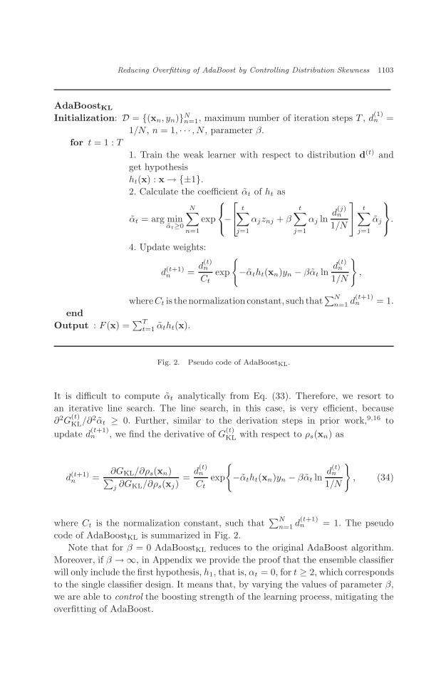
AdaBoostKL

Initialization: D = {(xn, yn)}Nn=1, maximum number of iteration steps T , d

(1)n =

1/N , n = 1, · · · , N , parameter β.for t = 1 : T

1. Train the weak learner with respect to distribution d(t) andget hypothesisht(x) : x → {±1}.2. Calculate the coefficient αt of ht as


N∑n=1

exp

− t∑

j=1

αjznj + βt∑

j=1

αj lnd(j)n

1/N

t∑j=1

αj

.

4. Update weights:

d(t+1)n =

d(t)n

Ctexp

{−αtht(xn)yn − βαt ln

d(t)n

1/N

},

whereCt is the normalization constant, such that∑N

n=1 d(t+1)n = 1.

endOutput : F (x) =

∑Tt=1 αtht(x).

Fig. 2. Pseudo code of AdaBoostKL.

It is difficult to compute αt analytically from Eq. (33). Therefore, we resort toan iterative line search. The line search, in this case, is very efficient, because∂2G

(t)KL/∂2αt ≥ 0. Further, similar to the derivation steps in prior work,9,16 to

update d(t+1)n , we find the derivative of G

(t)KL with respect to ρs(xn) as

d(t+1)n =

∂GKL/∂ρs(xn)∑j ∂GKL/∂ρs(xj)

=d(t)n

Ctexp

{−αtht(xn)yn − βαt ln

d(t)n

1/N

}, (34)

where Ct is the normalization constant, such that∑N

n=1 d(t+1)n = 1. The pseudo

code of AdaBoostKL is summarized in Fig. 2.Note that for β = 0 AdaBoostKL reduces to the original AdaBoost algorithm.

Moreover, if β → ∞, in Appendix we provide the proof that the ensemble classifierwill only include the first hypothesis, h1, that is, αt = 0, for t ≥ 2, which correspondsto the single classifier design. It means that, by varying the values of parameter β,we are able to control the boosting strength of the learning process, mitigating theoverfitting of AdaBoost.



3.3. AdaBoostnorm2

As discussed in Introduction, by employing different convex penalty terms to theobjective function of the minimax problem in Eq. (10), we can derive various typesof the soft margin, resulting in different regularized AdaBoost algorithms. In thissection, we consider the lp norm, ‖d − d(1)‖p , as the penalty function, which isa convex function of d. More specifically, we focus only on the l2 norm; however,generalization of the derivation steps below is straightforward.

Similar to the derivations in Sec. 3.2, from the optimization problem in Eq. (17),we obtain the following regularized scheme in the dual domain:

min(γ,d∈ΓN) γ + β‖d− d0‖2,

subject toN∑

n=1

dnznj ≤ γ, j = 1, . . . , |H|(35)

which can be linearly approximated as

min(γ,d∈ΓN) γ,

subject to zT.td ≤ γ, t = 1, . . . , T,

(36)

where z.t is the tth column of the new gain matrix, Z, defined as

Z = Z + β

[d(1) − d0

‖d(1) − d0‖2, . . . ,

d(T ) − d0

‖d(T ) − d0‖2

]. (37)

The dual form of Eq. (36) reads

max(ρ,α∈ΓT ) ρ,

subject toT∑

t=1

αtznt + βT∑

t=1

αtd(t)n − 1/N

‖d(t) − d0‖2≥ ρ, n = 1, . . . , N,

(38)

which gives rise to the soft margin of pattern xn, ρs(xn), defined as

ρs(xn) =T∑

t=1

αtznt + β

T∑t=1

αtd(t)n − 1/N

‖d(t) − d0‖2. (39)

Similar to the discussion in Sec. 3.2, β∑T

t=1 αtd(t)

n −1/N

‖d(t)−d0‖2can be interpreted

as “mistrust” in samples with respect to the center distribution. The term in thedenominator, ‖d(t) − d0‖2, can be roughly understood as follows: the closer thequery distribution to the center distribution, the more trust the outcome of thehypothesis deserves. Interestingly, the soft margin in Eq. (39) resembles that ofAdaBoostReg,14 defined as

ρReg(xn) =T∑

t=1

αtznt + βT∑

t=1

αtd(t)n . (40)

Obviously, from Eqs. (39) and (40), the main difference is that our soft margin iscomputed with respect to the center distribution.



Now, following the same strategy used in deriving AdaBoostKL, we reformulatethe optimization problem in Eq. (38) into an AdaBoost-like algorithm, which wecall AdaBoostnorm2. To this end, we define a new cost function, Gnorm2, as

Gnorm2 =N∑

n=1

exp

{−[∑

t

αtznt + β∑

t

αtd(t)n − 1/N

‖d(t) − d0‖2

]∑t

αt

}. (41)

To minimize the cost function, in each iteration step t, we first find ht as theone minimizing the weighted training error, and then calculate the combinationcoefficient αt as


G(t)norm2

= arg minαt≥0

N∑n=1

exp

− t∑

j=1

αjznj + β

t∑j=1

αjd(j)n − 1/N

‖d(j) − d0‖2

t∑j=1

αj

. (42)

The updated distribution d(t+1)(xn) is computed as the derivative of Gnorm2 withrespect to ρs(xn)

d(t+1)n =

∂G/∂ρs(xn)∑j ∂G/∂ρs(xj)

=d(t)n

Ctexp

{−αtht(xn)yn − βαt

d(t)n − 1/N

‖d(t) − d0‖2

}, (43)

where Ct is the normalization constant, such that∑N

n=1 d(t+1)n = 1. The pseudo

code of AdaBoostnorm2 is summarized in Fig. 3.

3.4. General framework

In this subsection, we summarize the proposed regularization of boosting algo-rithms by constraining their data distributions d. The general formulation of suchregularization can be specified as the following optimization problem in the dualdomain:

min(γ,dΓN ) γ + β(P )P (d)

subject to zT.jd ≤ γ, j = 1, . . . , |H| ,

(44)

where P (d) is a penalty function, and β(P ) is a function of P (d).Depending on the specification of P (d) and β(P ), it is possible to derive a

range of regularized boosting algorithms. For example, if β(P ) = β is a predefinedconstant, and P (d) is the KL divergence, or Euclidean distance between d andthe center distribution d0, we obtain AdaBoostKL or AdaBoostNorm2, respectively.Then, if we specify P (d) = ‖d‖∞, and β(P ) = 0 if P ≤ C, and β(P ) = ∞ ifP > C, we get LPreg-AdaBoost. We point out that this is a novel interpretation ofLPreg-AdaBoost. Note that both ν−Arc and C-Barrier algorithms, although beingimplemented in a different manner than the above algorithms, also fall into thiscategory.



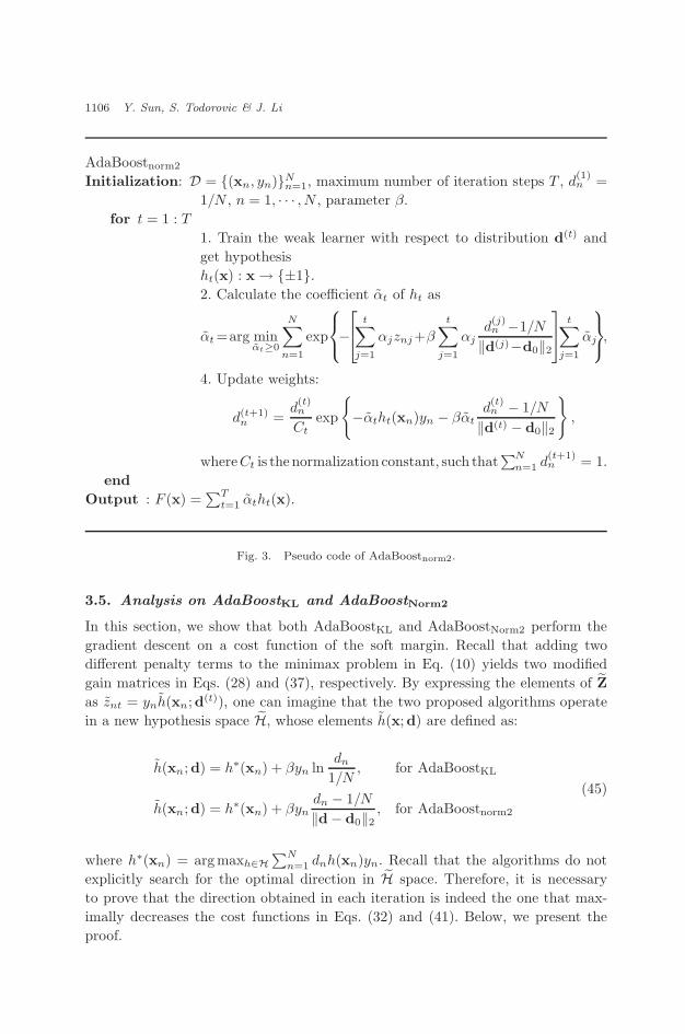
AdaBoostnorm2

Initialization: D = {(xn, yn)}Nn=1, maximum number of iteration steps T , d

(1)n =

1/N , n = 1, · · · , N , parameter β.for t = 1 : T

1. Train the weak learner with respect to distribution d(t) andget hypothesisht(x) : x → {±1}.2. Calculate the coefficient αt of ht as

αt =arg minαt≥0

N∑n=1

exp

− t∑

j=1

αjznj+βt∑

j=1

αjd(j)n −1/N

‖d(j)−d0‖2

t∑j=1

αj

,

4. Update weights:

d(t+1)n =

d(t)n

Ctexp

{−αtht(xn)yn − βαt

d(t)n − 1/N

‖d(t) − d0‖2

},

whereCt is the normalization constant, such that∑N

n=1 d(t+1)n = 1.

endOutput : F (x) =

∑Tt=1 αtht(x).

Fig. 3. Pseudo code of AdaBoostnorm2.

3.5. Analysis on AdaBoostKL and AdaBoostNorm2

In this section, we show that both AdaBoostKL and AdaBoostNorm2 perform thegradient descent on a cost function of the soft margin. Recall that adding twodifferent penalty terms to the minimax problem in Eq. (10) yields two modifiedgain matrices in Eqs. (28) and (37), respectively. By expressing the elements of Zas znt = ynh(xn;d(t)), one can imagine that the two proposed algorithms operatein a new hypothesis space H, whose elements h(x;d) are defined as:

h(xn;d) = h∗(xn) + βyn lndn

1/N, for AdaBoostKL

h(xn;d) = h∗(xn) + βyndn − 1/N

‖d− d0‖2, for AdaBoostnorm2

(45)

where h∗(xn) = argmaxh∈H∑N

n=1 dnh(xn)yn. Recall that the algorithms do notexplicitly search for the optimal direction in H space. Therefore, it is necessaryto prove that the direction obtained in each iteration is indeed the one that max-imally decreases the cost functions in Eqs. (32) and (41). Below, we present theproof.



We first consider AdaBoostKL. From Eq. (32), after the (t − 1)th iteration,we have

G(t−1)KL =

N∑n=1

exp

−yn

t−1∑j

αj hj(xn)

. (46)

In the tth iteration, the optimal direction ht(xn) in which the cost function mostrapidly decreases, subject to ht(xn) ∈ H, is computed, such that the inner product

〈−∇G(t−1)KL , ht(xn)〉 ∝

N∑n=1

d(t)n ynht(xn) =

N∑n=1

d(t)n ynht(xn) + β

N∑n=1

d(t)n ln

dn

1/N

(47)

is maximized, similar to the derivation in Sec. 2. It is straightforward to prove thatEq. (47) attains the maximum when ht(x) = h(x;d(t)), that is, when d = d(t),which follows from the well-known properties of the KL divergence.3

In the case of AdaBoostnorm2, by following the derivation steps in Sec. 2, wearrive at a similar expression to that in Eq. (47). To show that in the tth iterationthe optimal direction ht(x) = h(x;d(t)), we only need to show that

∑n d

(t)n

(dn−1/N)‖d−d0‖2

is maximized when d = d(t):(d− d0)T

‖d− d0‖2d(t) =

(d − d0)T(d(t) − d0)‖d− d0‖2

≤ |(d− d0)T(d(t) − d0)|‖d− d0‖2

≤ ‖d(t) − d0‖2.

(48)

From the Cauchy–Schwartz inequality, the equality in Eq. (48) holds when d = d(t).This completes the proof.

In summary, AdaBoostKL and AdaBoostNorm2 perform the stage-wise gradientdescent in the new hypothesis space H instead of in H. The new hypothesis space,H, encodes the information on the data distribution skewness with respect to thecenter distribution. From Eq. (45), it follows that for implementation of the twoalgorithms it is not necessary to explicitly construct H.

Considering our discussion in Sec. 3.1, one may also construct a similar newhypothesis space for AdaBoostReg. However, AdaBoostReg cannot be explained asa gradient-descent algorithm in that space, because the direction the algorithmsearches for in each iteration is not the one that maximally decreases the associatedcost function.

4. Experimental Results

We report the results of a large scale experiment, where the proposed algorithmsare compared with AdaBoostReg, ν-Arc, C-Barrier, RBF (radial basis function),and SVM (RBF kernel). For fairness sake, our experimental setup is the same asthe one used for evaluation of AdaBoostReg by Ratsch et al.16 We use 13 artificialand real-world data sets originally from the UCI, DELVE and STATLOG bench-mark repositions: banana, breast cancer, diabetis, flare solar, german, heart, image



(a)

(b)

Fig. 4. (a) Illustration of the optimization problem in Eq. (21) in the case of |H| = 2. (γ∗, d∗)is the optimum solution; (b) Linear approximation of Eq. (21). (γ∗, d∗) is obtained by solvingEq. (29), which is the approximate solution to the original problem.

ringnorm, splice, thyroid, titanic, twonorm, and waveform. Each data set has 100realizations of training and testing data. For each realization, a classifier is trainedand the test error is computed. The detailed information about the experimentalsetup and the benchmark data sets can also be found in Ref. 15.

The RBF net is used as the weak learner. All of the RBF parameters are thesame as those used in Ref. 16. To avoid repeating the report on the numerous RBFparameters, for details we refer the reader to Ref. 16. We use cross-validation toestimate the optimal parameter β. The maximum number of iterations, T , is chosento be 200.

Below, we present several tests, which illustrate the properties of the proposedalgorithms. First, we show classification results on banana data set, whose samplesare characterized by two features. In Fig. 5, we plot the decision boundaries of



Sunfletflalfl

-3 -2 -1 0 1 2 3-3

-2

-1

0

1

2

3Decision Boundary (AdaBoost)

0

0

0

0

0

0

0

00

0

0

0

00

-3 -2 -1 0 1 2 3-3

-2

-1

0

1

2

3Decision Boundary(AB-KL)

0

0

0

00

00

0

0

(a) (b)

-3 -2 -1 0 1 2 3-3

-2

-1

0

1

2

3Decision Boundary(AB-KL)

0

0

0

00

00

0

0

(c)

Fig. 5. The decision boundaries of three methods: AdaBoost, AdaBoostnorm2 and AdaBoostKL

based on one realization of the banana data. AdaBoost tries to classify each pattern according toits associated label and forms a zigzag decision boundary, which gives a straightforward illustrationof the overfitting phenomenon of AdaBoost. Both AdaBoostnorm2 and AdaBoostKL give smoothand similar decision boundaries.

AdaBoost, AdaBoostnorm2, and AdaBoostKL in the two-dimensional feature space.From the figure, it is obvious that AdaBoost tries to classify each pattern cor-rectly according to its associated label, forming a zigzag shaped decision boundary,which indicates the overfitting of AdaBoost. In contrast, both AdaBoostnorm2 andAdaBoostKL produce smooth decision boundaries by ignoring some hard-to-learnsamples. Note that the boundaries of our algorithms are very similar.

Second, we present the classification results, and margin plots of three methods:AdaBoost, AdaBoostnorm2, and AdaBoostKL, on one realization of the waveformdata. From Figs. 6(a) and 6(b), we observe that AdaBoost tries to maximize themargin, thereby effectively reducing the training error to zero; however, it also



0 50 100 150 2000

0.02

0.04

0.06

0.08

0.1

0.12Results(AdaBoost)

iteration number

clas

sific

atio

n er

ror

TrainTest

20 40 60 80 100 120 140 160 180 200-1.5

-1

-0.5

0

0.5

1Margin(AdaBoost)

iteration numberm

argi

n

Margin

(a) (b)

0 50 100 150 2000.065

0.07

0.075

0.08

0.085

0.09

0.095

0.1

0.105

0.11Results(AB-KL)

iteration number

clas

sific

atio

n er

ror

TrainTest

20 40 60 80 100 120 140 160 180 200-1.5

-1

-0.5

0

0.5

1

Margin(AdaBoostKL

)

iteration number

mar

gin

Hard MarginSoft Margin

(c) (d)

0 50 100 150 2000.04

0.05

0.06

0.07

0.08

0.09

0.1

0.11Results(AB-Norm2)

iteration number

clas

sific

atio

n er

ror

TrainTest

20 40 60 80 100 120 140 160 180 200-1.5

-1

-0.5

0

0.5

1

Margin(AdaBoostNorm2

)

iteration number

mar

gin

Hard MarginSoft Margin

(e) (f)

Fig. 6. Training and testing results, and margin plots of three methods: AdaBoost,AdaBoostnorm2 and AdaBoostKL based on the waveform data. AdaBoost quickly leads to over-fitting while the regularized methods effectively alleviate this problem.



Table

1.

Cla

ssifi

cati

on

erro

rsand

standard

dev

iati

ons

ofei

ght

alg

ori

thm

s.

RB

FA

BA

BR

AB

KL

AB

norm

2ν

Arc

C-B

ar

SV

M

wave

form

10.7

±1.1

10.8

±0.6

9.8

±0.8

9.4

±0.6

9.5

±0

.410.0

±0.7

9.7

±0.5

9.9

±0.4

thyro

id4.5

±2.1

4.4

±2

.24.6

±2.2

4.3

±1.9

4.4

±2

.24

.4±

2.2

4.5

±2.2

4.8

±2.2

banana

10.8

±0.6

12.3

±0.7

10.9

±0.4

10.7

±0.4

10.6

±0.4

10.8

±0.5

10.9

±0.5

11.5

±0.7

Bca

nce

r27.6

±4.7

30.4

±4.7

26.5

±4.5

26.1

±4.4

26.0

±4.4

25.8

±4.6

25

.9±

4.4

26.0

±4.7

dia

betis

24.3

±1.9

26.5

±2.3

23.8

±1.8

23.5

±1.8

23.6

±1.8

23.7

±2.0

23.7

±1.8

23.5

±1.7

germ

an

24.7

±2.4

27.5

±2.5

24.3

±2.1

24.2

±2.2

24.1

±2.2

24.4

±2.2

24.3

±2.4

23.6

±2.1

hea

rt17.6

±3.3

20.3

±3.4

16.5

±3.5

16.9

±3.2

17.0

±3.1

16.5

±3.5

17.0

±3.4

16.0

±3.3

ringn

orm

1.7

±0.2

1.9

±0.3

1.6

±0.1

1.5

±0.1

1.6

±0.1

1.7

±0.2

1.7

±0.2

1.7

±0.1

Fso

lar

34.4

±2.0

35.7

±1.8

34.2

±2.2

34.1

±1.6

34.1

±1.7

34.4

±1.9

33.7

±1.9

32.4

±1.8

tita

nic

23.3

±1.3

22.6

±1.2

22.6

±1.2

22

.5±

0.9

22

.5±

1.2

23.0

±1.4

22.4

±1.1

22.4

±1.0

splice

10.0

±1.0

10.1

±0.5

9.5

±0.7

9.2

±0.6

9.5

±0.5

N/A

N/A

10.9

±0.7

image

3.3

±0.6

2.7

±0.7

2.7

±0.6

2.7

±0.6

2.7

±0.5

N/A

N/A

3.0

±0.6

twonorm

2.9

±0.3

3.0

±0.3

2.7

±0

.22.6

±0.2

2.7

±0

.2N

/A

N/A

3.0

±0.2



Table 2. 90% significant test comparing AdaBoostKL with the other algorithms.

ABKL/RBF ABKL/AB ABKL/ABR ABKL/νArc ABKL/C-Bar ABKL/SVM

waveform + + + + + +thyroid 0 0 0 0 0 +banana + + + + + +Bcancer + + 0 0 0 0diabetis + + 0 0 0 0german + + 0 0 0 −heart 0 + 0 0 0 −ringnorm + + + + + +Fsolar 0 + 0 0 0 −titanic + 0 0 0 0 0splice + + + N/A N/A +Image + 0 0 N/A N/A +twonorm + + + N/A N/A +

quickly leads to overfitting. It is reported that the simple early stopping methodcould alleviate the overfitting of AdaBoost. However, in this example (and manyother examples on other data sets) we find that the early stopping method is notapplicable. In contrast to AdaBoost, AdaBoostnorm2 and AdaBoostKL try to max-imize the soft margin, allowing a few hard-to-learn samples to have a small (evennegative) sample margin. The two regularized algorithms effectively overcome theoverfitting problem.

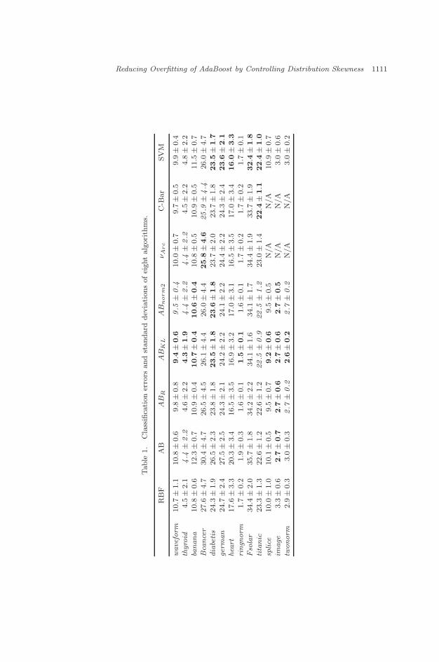
For a more comprehensive comparison, in Table 1, we provide the average clas-sification results, with standard deviations, over the 100 realizations of the 13 datasets. The best results are marked in boldface, while the second best, in italics. Byanalyzing the results in Table 1, we conclude the following:

• AdaBoost performs worse than a single RBF classifier in almost all cases, due tothe overfitting of AdaBoost. In ten out of thirteen cases AdaBoostReg performssignificantly better than AdaBoost, and in ten cases AdaBoostReg outperforms asingle RBF classifier.

• Except for heart, both AdaBoostnorm2 and AdaBoostKL prove better thanAdaBoostReg.

• In comparison with ν-Arc and C-Barrier, our algorithms also perform better inmost cases. This may be explained due to a hard limited penalty function usedin the underlying optimization scheme of ν-Arc and C-Barrier.

• In almost all cases, the standard deviations of AdaBoostnorm2 and AdaBoostKL

are smaller than those of the single RBF classifier and AdaBoost.• The results for ringnorm, thyroid and twonorm suggest that the regularized

AdaBoost algorithms are effective even in the low noise regime.

For a more rigorous comparison, a 90% significant test is reported in Table 2.In the table, ‘0’ means the test accepts the null hypothesis:“no significant differ-ence in average performance”; ‘+’ denotes the test accepts the alternative hypoth-esis: “AdaBoostKL is significantly better”; finally, ‘−’ indicates: “AdaBoostKL



is significantly worse”. For some data sets the performance differences betweenAdaBoostKL and AdaBoostReg are small (e.g. titanic). This is because AdaBoostReg

is already a good classifier, which has been reported to be slightly better than Sup-port Vector Machine (RBF kernel).16 Nevertheless, significant improvements areobserved for AdaBoostKL in five datasets out of thirteen (Table 2).

5. Conclusions

In this paper, we have studied strategies to regularize AdaBoost, in order to reduceits overfitting, which has been reported to occur in high-noise regimes. By exploitingthe connection between the minimax optimization problem, and the AdaBoost algo-rithm, we have explained that the impressive generalization capability of AdaBoostin low-noise settings may stem from the fact that the ensemble classifier tries tooptimize the performance in the worst case. Due to this very mechanism, we spec-ulate the overfitting of AdaBoost is inevitable in noisy data cases.

We have proposed to alleviate the problem by penalizing the data distributionskewness in the learning process. In this manner, a few outlier samples are pre-vented from spoiling decision boundaries. More specifically, to control the skewness,we have proposed to add a convex penalty function to the objective of the mini-max problem. By means of the generalized minimax theorem, we have shown thatthe regularization scheme can be pursued equivalently in the dual domain, whereinwe have specified the general framework of the proposed regularization. This gen-eral framework gives rise to a range of regularized boosting algorithms, differingin a particular specification of the penalty function. Thus, we have pointed outthat LPreg-AdaBoost can be derived from the outlined framework if the penalty isdefined as a hard-limited function, which represents a novel interpretation of thealgorithm.

We have proposed to use two smooth convex penalty functions, one based on theKL divergence and the other on the Euclidean distance between the query and thecenter data distribution; thereby, we have derived two novel regularized algorithmsAdaBoostKL and AdaBoostnorm2, respectively. We have proved that the proposedalgorithms perform a stage-wise gradient-descent procedure on the cost function ofthe corresponding soft margin.

We have demonstrated the effectiveness of our algorithms by conducting exper-iments on a wide variety of data. In comparison with AdaBoostReg, ν-Arc, andC-Barrier, our AdaBoostKL and AdaBoostNorm2 achieve at least the same, or bet-ter classification performance.

Appendix A. Appendices

Lemma 1. Suppose in each iteration the learning algorithm can find a hypothesissuch that Eq. (27) holds. If β → ∞, only the first hypothesis h1 will be kept inAdaBoostKL, i.e. αt = 0, for t ≥ 2.



Proof. Suppose AdaBoostKL found h1 and the corresponding combination coeffi-cient α1. Also, suppose it found h2, as well, and it is about to determine α2 by aline search. The intermediate cost function is given by:

G(2)KL =

N∑n=1

exp(−F1(xn)yn) exp{−α2h2(xn)yn − α2β ln(d(2)

n N)}

=N∑

j=1

exp (−F1(xj)yj)N∑

n=1

d(2)n exp

{−α2h2(xn)yn − α2β ln(d(2)

n N)}

.

α2 can be computed by taking a derivative of G(2)KL with respect to α2, and setting

it to zero. For simplicity, we drop the constant terms.

∂G(2)KL/∂α2

=N∑

n=1

d(2)n exp

{−α2h2(xn)yn − α2β ln(d(2)

n N)}{

−h2(xn)yn − β ln(d(2)n N)

}

=N∑

n=1

d(2)n exp(−α2h2(xn)yn) (d(2)

n N)−α2β{−h2(xn)yn − β ln(d(2)

n N)}

= 0.

By setting α2 = 1/β and letting β → ∞, we have:

limβ→∞

∂G(2)KL/∂α2 = lim

β→∞

N∑n=1

1N

exp(−h2(xn)yn

β

){−h2(xn)yn − β ln(d(2)

n N)}

> 0.

The last inequality follows from the fact that∑N

n=11N ln(d(2)

n N) < 0 for d(2) �= d0.By setting α2 = 1/β2 and letting β → ∞, we have:

limβ→∞

∂G(2)KL/∂α2

= limβ→∞

N∑n=1

(d(2)n )1−1/βN−1/β exp

(−h2(xn)yn

β2

){−h2(xn)yn − β ln(d(2)

n N)}

< 0.

The last inequality follows from the fact that∑N

n=1 d(2)n ln(d(2)

n N) > 0 for d(2) �= d0.Therefore, when β → ∞, α2 ∈ ( 1

β2 , 1β ) → 0.

References

1. L. Breiman, Prediction games and arcing algorithms, Neural Comput. 11 (1999)1493–1517.

2. C. Cortes and V. Vapnik, Support vector networks, Mach. Learn. 20 (1995) 273–297.3. T. M. Cover and J. A. Thomas, Elements of Information Theory (Wiley Interscience

Press New York, 1991).4. A. Demiriz, K. P. Bennett and J. Shawe-Taylor, Linear programming boosting via

column generation, Mach. Learn. 46 (2002) 225–254.



5. T. G. Dietterich, An experimental comparison of three methods for constructingensembles of decision trees: bagging, boosting, and randomization, Mach. Learn. 40(2000) 139–157.

6. I. Ekeland and R. Temam, Convex Analysis and Variational Problems (North-HollandPub. Co., Amsterdam, 1976)

7. Y. Freund and R. E. Schapire, Game theory, on-line prediction and boosting, Proc.Ninth Annual Conf. Computational Learning Theory (1996).

8. Y. Freund and R. E. Schapire, A decision-theoretic generalization of on-line learningand an application to boosting, in Eurp. Conf. Computational Learning Theory (1995),pp. 23–37.

9. J. Friedman, Greedy function approximation: a gradient boosting machine, Ann.Statis. 29(5) (2001) 1189–1232.

10. A. J. Grove and D. Schuurmans, Boosting in the limit: maximizing the margin oflearned ensembles, AAAI/IAAI (1998), pp. 692–699.

11. L. Mason, J. Bartlett, P. Baxter and M. Frean, Functional gradient techniques forcombining hypotheses, in Advances in Large Margin Classifiers, eds. B. Scholkopf,A. Smola, P. Bartlett and D. Schuurmans (2000).

12. R. Meir and G. Ratsch, An introduction to boosting and leveraging, in AdvancedLectures on Machine Learning, eds. S. Mendelson and A. Smola (Springer, 2003),pp. 119–184.

13. S. G. Nash and A. Sofer, Linear and Nonlinear Programming (McGraw-Hill, NY,USA, 1996), Chap. 7.4.

14. G. Ratsch, Robust Boosting via Convex Optimization: Theory and Application, Ph.D.thesis, University of Potsdam, Germany (October 2001).

15. G. Ratsch, IDA benchmark repository, World Wide Web, http://ida.first.fhg.de/projects/bench/benchmarks.htm (2001).

16. G. Ratsch, T. Onoda and K.-R. Muller, Soft margins for AdaBoost, Mach. Learn. 42(2001) 287–320.

17. G. Ratsch, B. Scholkopf, A. Smola, S. Mika, T. Onoda and K.-R. Muller, Robustensemble learning, in Advances in Large Margin Classifiers, eds. B. Scholkopf,A. Smola, P. Bartlett and D. Schuurmans (2000), pp. 207–220.

18. C. Rudin I. Daubechies and R. E. Schapire, The dynamics of adaboost: cyclic behaviorand convergence of margins, J. Mach. Learn. Res. 5 (2004) 1557–1595.

19. R. E. Schapire, Y. Freund, P. Bartlett and W. S. Lee, Boosting the margin: a newexplanation for the effectiveness of voting methods, Proc. 14th Int. Conf. MachineLearning (1997), pp. 322–330.

20. R. E. Schapire, Y. Freund, P. Bartlett and W. S. Lee, Boosting the margin: a new expla-nation for the effectiveness of voting methods, Ann. Statis. 26(5)(1998) 1651–1686.

21. R. Schapire and Y. Singer, Improved boosting algorithms using confidence-rated pre-dictions, Mach. Learn. 37(3) (1999) 297–336.

22. V. Vapnik, Statistical Learning Theory (John Wiley and Sons Inc., New York, 1998).23. J. von Neumann, Zur theorie der gesellschaftsspiele, Math. Ann. 100 (1928) 295–320.



Yijun Sun received theB.S. degrees in bothelectrical and mechan-ical engineering fromShanghai Jiao TongUniversity, Shanghai,China, in 1995, and theM.S. and Ph.D. degreesin electrical engineeringfrom the University of

Florida, Gainesville, USA, in 2003 and 2004,respectively. Since 2000, he has been aresearch assistant at the Department of Elec-trical and Computer Engineering at the Uni-versity of Florida. Currently, he is a researchscientist at the Interdisciplinary Center forBiotechnology Research at the University ofFlorida. He also holds a position of visitingassistant professor at the Department of Elec-

trical and Computer Engineering at the sameuniversity.

His research interests include patternrecognition, machine learning, statistical sig-nal processing, and their applications to tar-get recognition and bioinformatics.

Jian Li received theM.Sc. and Ph.D. degreesin electrical engineer-ing from the Ohio StateUniversity, Columbus,in 1987 and 1991, respec-tively.

From April 1991 toJune 1991, she was anAdjunct Assistant Pro-

fessor with the Department of Electri-cal Engineering, the Ohio State University,Columbus. From July 1991 to June 1993, shewas an Assistant Professor with the Depart-ment of Electrical Engineering, University ofKentucky, Lexington. Since August 1993, shehas been with the Department of Electri-cal and Computer Engineering, University ofFlorida, Gainesville, where she is currently a

Professor.Her current research interests include spec-

tral estimation, statistical and array signalprocessing, and their applications.

Dr. Li is a Fellow of IEEE and a Fel-low of IEE. She is a member of SigmaXi and Phi Kappa Phi. She received the1994 National Science Foundation YoungInvestigator Award and the 1996 Office ofNaval Research Young Investigator Award.She was an Executive Committee Member ofthe 2002 International Conference on Acous-tics, Speech, and Signal Processing, Orlando,Florida, May 2002. She was an AssociateEditor of the IEEE Transactions on SignalProcessing from 1999 to 2005 and an Asso-ciate Editor of the IEEE Signal ProcessingMagazine from 2003 to 2005. She has been amember of the Editorial Board of Signal Pro-cessing, a publication of the European Associ-ation for Signal Processing (EURASIP), since2005. She is presently a member of two ofthe IEEE Signal Processing Society technicalcommittees: the Signal Processing Theoryand Methods (SPTM) Technical Commit-tee and the Sensor Array and Multichannel(SAM) Technical Committee.

Sinisa Todorovic rece-ived his B.S. degree inelectrical engineering atthe University of Bel-grade, Serbia, in 1994.From 1994 until 2001,he worked as a softwareengineer in the commu-nications industry. Heearned his M.S. and

Ph.D. degrees at the University of Florida,in 2002, and 2005, respectively. Currently, heholds the position of postdoctoral researchassociate at Beckman Institute, University ofIllinois at Urbana-Champaign.

His primary research interests encompassstatistical image modeling for object recogni-tion and image segmentation, machine learn-ing, and multi-resolution image processing.He has published approximately 20 journaland refereed conference papers.

Documents

REDUCING THE OVERFITTING OF ADABOOST BY …web.engr.oregonstate.edu/~sinisa/research/publications/IJPRAI06.pdf · November 10, 2006 14:11 WSPC/115-IJPRAI SPI-J068 00513 Reducing Overﬁtting