Embed Size (px)
Citation preview
SRM UNIVERSITY
EE0311-Measurements & Control System Lab 1
REFERENCE MANUAL
EE0311 – MEASUREMENTS & CONTROL SYSTEMS LAB
DEPARTMENT OF ELECTRICAL & ELECTRONICS ENGINEERING FACULTY OF ENGINEERING & TECHNOLOGY
SRM UNIVERSITY, Kattankulathur – 603 203
SRM UNIVERSITY
EE0311-Measurements & Control System Lab 2
LIST OF EXPERIMENTS
Sl.No. Name of the Experiments Page No.
1 Measurements of Inductance using Maxwell’s bridge
2 Measurements of Inductance using Anderson’s bridge
3 Measurements of capacitance Schering’s bridge
4 Measurements of resistance using whetstone bridge
5 Measurements of resistance using Kelvin’s bridge
6 Calibration of single phase energy meter direct loading
7 Calibration of single energy meter Phantom loading
8 Calibration of three phase energy meter direct loading
9 Measurements of power factors
10 Study of synchro transmitter & receiver pair
11 Speed torque characteristics AC servo motor
12 Transfer function field controlled DC motor
13 Design and implementation of Lag, Lead compensator
14 Transfer function of armature controlled DC motor
15 Digital simulation of the above controller using MATLAB
software
SRM UNIVERSITY
EE0311-Measurements & Control System Lab 3
Exp. No.1
MAXWELL’S CAPACITANCE BRIDGE
Aim
To measure the
i) Inductance of a coil
ii) Q factor of the coil using Maxwell’s bridge
Apparatus Required
Sl.No. Apparatus Range Quantity
1 Maxwell’s bridge kit -- 1
2 Inductive coil -- 1
3 Headphone -- 1
Theory
In this bridge, an inductance is measured by comparison with a standard variable
capacitance
Under balanced condition
32
44
411
1)( RR
RCj
RLjR
R1R4 + j L1R4 = R2R3 + j R2R3C4R4
Separating the real and imaginary parts,
R1 = 4
32
R
RR
and L1 = R2R3C4
The expression for Q factor of the coil is, Q = L1 / R1 = C4R4
Formula Used
L1 = Unknown inductance – Henry
R2 = Non inductive resistance – ohms
Rm = Multiplier resistance – ohms
C1 = 0.1F

SRM UNIVERSITY
EE0311-Measurements & Control System Lab 4
Procedure
Connection to be made as per the circuit diagram
The balance condition is obtained by adjusting capacitance in the bridge
The balanced condition is checked with a help of headphone
All the values in the bridge are noted down
MAXWELL’S BRIDGE
L1 – Unknown inductance
R1 – Effective resistance of inductor,
C4 – Variable standard capacitor
R2, R3, R4 – Known non-inductive resistance
Phasor Diagram
E3 = E4 = I1 R3 = I4 R4 = IC / C4
SRM UNIVERSITY
EE0311-Measurements & Control System Lab 5
Tabulation
Maxwell’s bridge method
Sr.
No.
Given Inductance
‘L’
Capacitance
‘C’
Resistance
‘Rm’
Resistance
R2’
L = PRC
Unit Henry F K K mH
1 600 0.6 1000 1000 600
2 520 0.5 1000 1000 500
3 550 0.6 1000 1000 600
Model calculation
P = 1000
R = 1000
C = 0.655 x 10⁻⁶
F
L = PRC
= 1000 1000 0.6 10-6
= 0.6
= 600 mH
Result
Thus the inductance of the given coil is found by Maxwell’s bridge
SRM UNIVERSITY
EE0311-Measurements & Control System Lab 6
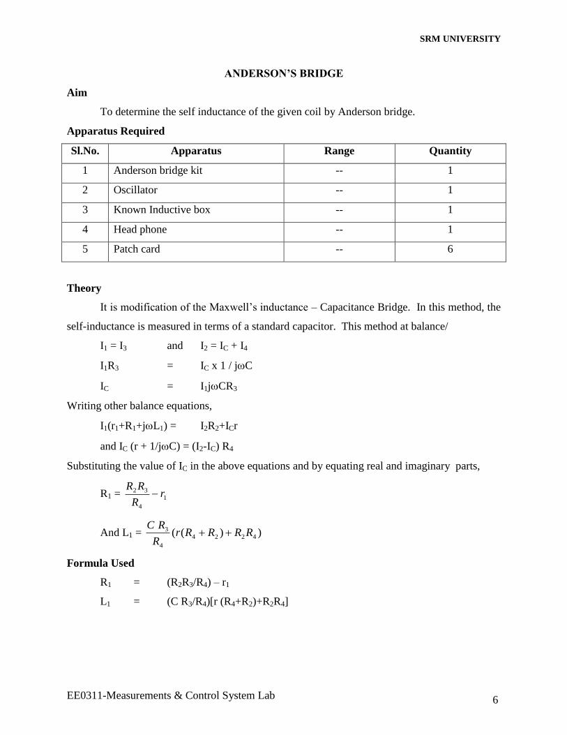
ANDERSON’S BRIDGE
Aim
To determine the self inductance of the given coil by Anderson bridge.
Apparatus Required
Sl.No. Apparatus Range Quantity
1 Anderson bridge kit -- 1
2 Oscillator -- 1
3 Known Inductive box -- 1
4 Head phone -- 1
5 Patch card -- 6
Theory
It is modification of the Maxwell’s inductance – Capacitance Bridge. In this method, the
self-inductance is measured in terms of a standard capacitor. This method at balance/
I1 = I3 and I2 = IC + I4
I1R3 = IC x 1 / jC
IC = I1jCR3
Writing other balance equations,
I1(r1+R1+jL1) = I2R2+ICr
and IC (r + 1/jC) = (I2-IC) R4
Substituting the value of IC in the above equations and by equating real and imaginary parts,
R1 = 1
4
32 rR
RR
And L1 = ))(( 4224
4
3 RRRRrR
RC
Formula Used
R1 = (R2R3/R4) – r1
L1 = (C R3/R4)[r (R4+R2)+R2R4]

SRM UNIVERSITY
EE0311-Measurements & Control System Lab 7
ANDERSON’S BRIDGE
Phasor Diagram
Procedure
Connection to be made as per the circuit diagram.
With a particular value of ‘C’ the balanced condition is obtained by adjusting the
value of resistance.
All the values in the bridge are noted down
Repeat it with different values of ‘C’ and calculate every time the value of ‘L’.
SRM UNIVERSITY
EE0311-Measurements & Control System Lab 8
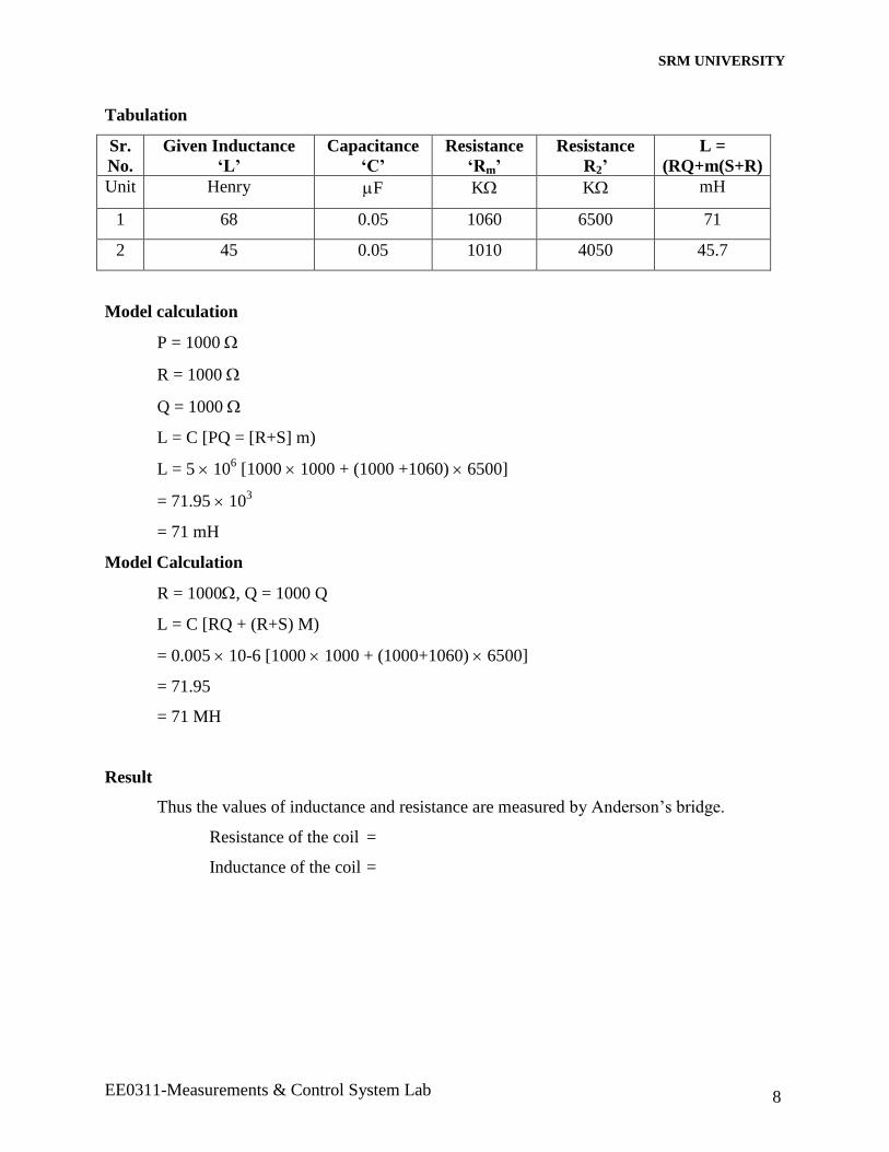
Tabulation
Sr.
No.
Given Inductance
‘L’
Capacitance
‘C’
Resistance
‘Rm’
Resistance
R2’
L =
(RQ+m(S+R)
Unit Henry F K K mH
1 68 0.05 1060 6500 71
2 45 0.05 1010 4050 45.7
Model calculation
P = 1000
R = 1000
Q = 1000
L = C [PQ = [R+S] m)
L = 5 106 [1000 1000 + (1000 +1060) 6500]
= 71.95 103
= 71 mH
Model Calculation
R = 1000, Q = 1000 Q
L = C [RQ + (R+S) M)
= 0.005 10-6 [1000 1000 + (1000+1060) 6500]
= 71.95
= 71 MH
Result
Thus the values of inductance and resistance are measured by Anderson’s bridge.
Resistance of the coil =
Inductance of the coil =
SRM UNIVERSITY
EE0311-Measurements & Control System Lab 9
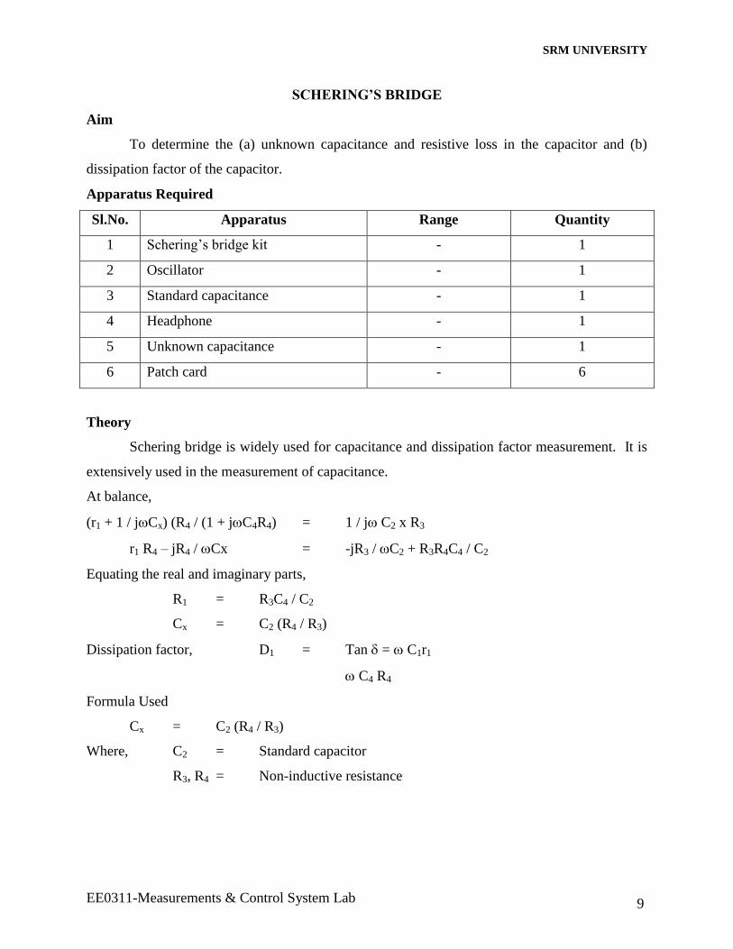
SCHERING’S BRIDGE
Aim
To determine the (a) unknown capacitance and resistive loss in the capacitor and (b)
dissipation factor of the capacitor.
Apparatus Required
Sl.No. Apparatus Range Quantity
1 Schering’s bridge kit - 1
2 Oscillator - 1
3 Standard capacitance - 1
4 Headphone - 1
5 Unknown capacitance - 1
6 Patch card - 6
Theory
Schering bridge is widely used for capacitance and dissipation factor measurement. It is
extensively used in the measurement of capacitance.
At balance,
(r1 + 1 / jCx) (R4 / (1 + jC4R4) = 1 / j C2 x R3
r1 R4 – jR4 / Cx = -jR3 / C2 + R3R4C4 / C2
Equating the real and imaginary parts,
R1 = R3C4 / C2
Cx = C2 (R4 / R3)
Dissipation factor, D1 = Tan = C1r1
C4 R4
Formula Used
Cx = C2 (R4 / R3)
Where, C2 = Standard capacitor
R3, R4 = Non-inductive resistance
SRM UNIVERSITY
EE0311-Measurements & Control System Lab 10
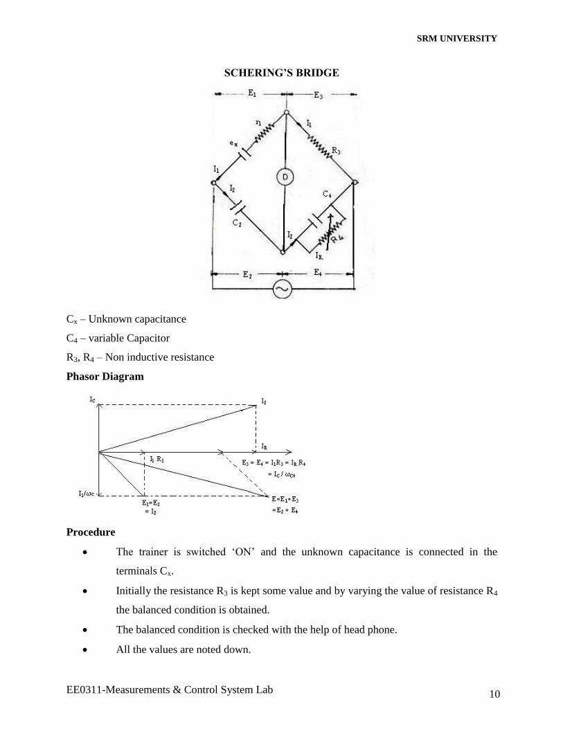
SCHERING’S BRIDGE
Cx – Unknown capacitance
C4 – variable Capacitor
R3, R4 – Non inductive resistance
Phasor Diagram
Procedure
The trainer is switched ‘ON’ and the unknown capacitance is connected in the
terminals Cx.
Initially the resistance R3 is kept some value and by varying the value of resistance R4
the balanced condition is obtained.
The balanced condition is checked with the help of head phone.
All the values are noted down.
SRM UNIVERSITY
EE0311-Measurements & Control System Lab 11
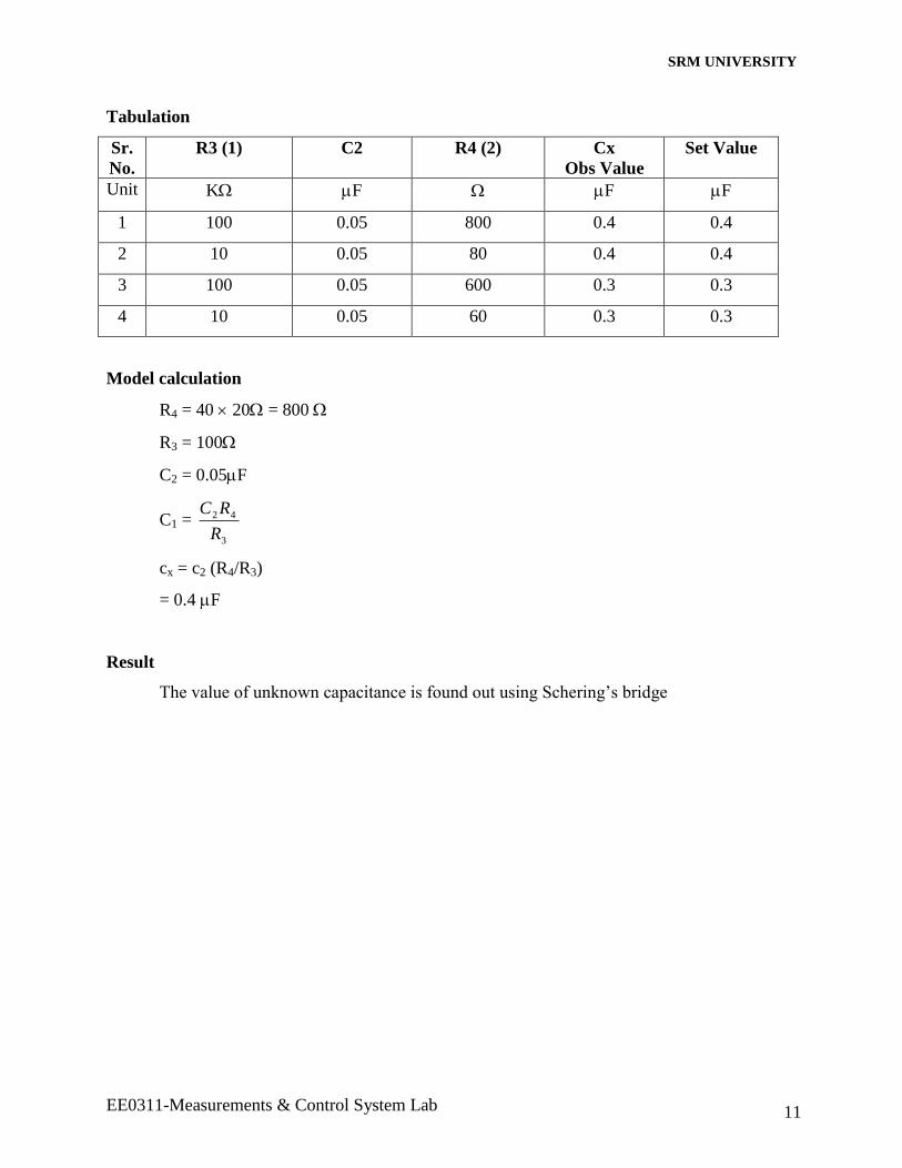
Tabulation
Sr.
No.
R3 (1) C2 R4 (2) Cx
Obs Value
Set Value
Unit K F F F
1 100 0.05 800 0.4 0.4
2 10 0.05 80 0.4 0.4
3 100 0.05 600 0.3 0.3
4 10 0.05 60 0.3 0.3
Model calculation
R4 = 40 20 = 800
R3 = 100
C2 = 0.05F
C1 = 3
42
R
RC
cx = c2 (R4/R3)
= 0.4 F
Result
The value of unknown capacitance is found out using Schering’s bridge
SRM UNIVERSITY
EE0311-Measurements & Control System Lab 12
MEASUREMENT OF RESISTANCE USING WHEATSTONE BRIDGE
Aim
To measure the given medium resistance using Wheatstone bridge.
Apparatus Required
Sl.No. Apparatus Range Quantity
1 Wheatstone bridge kit -- 1
2 Unknown resistance -- 1
3 Galvanometer -- 1
4 Patch card -- 6
Theory
It is used for the measurement of medium resistances. Very high degrees of accuracy can
be achieved with the Wheatstone bridge. It has four resistive arms, consisting of resistances R1,
R2, R3 and R4 together with a battery source and a null detector usually a galvanometer or other
sensitive current meter. The current through the galvanometer depends on the potential
difference between points C and D. The bridge is said to be balanced when there is no current
through the galvanometer or when the potential difference across the galvanometer is zero.
For bridge balance we can write,
I1 R1 = I2 R2 (1)
For galvanometer current to be zero, the following conditions also exist:
41
31RR
EII
(2)
And 32
42RR
EII
(3)
Combining the above three equations
321
2
41
1
RR
R
RR
R
R2 R4 = R1R3
From which,
2
31
4R
RRR
SRM UNIVERSITY
EE0311-Measurements & Control System Lab 13
Formula Used
Unknown resistance 2
31
R
RRRx
Where 2
3
R
R= ratio arm.
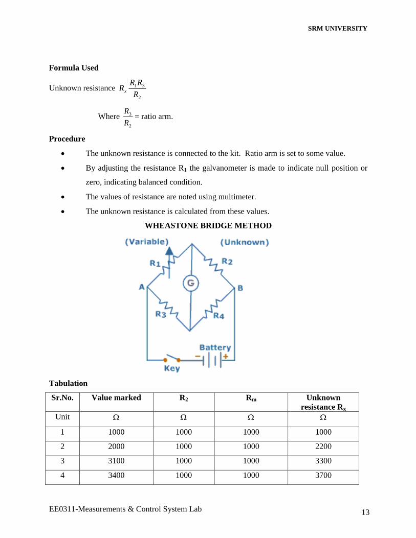
Procedure
The unknown resistance is connected to the kit. Ratio arm is set to some value.
By adjusting the resistance R1 the galvanometer is made to indicate null position or
zero, indicating balanced condition.
The values of resistance are noted using multimeter.
The unknown resistance is calculated from these values.
WHEASTONE BRIDGE METHOD
Tabulation
Sr.No. Value marked R2 Rm Unknown
resistance Rx
Unit
1 1000 1000 1000 1000
2 2000 1000 1000 2200
3 3100 1000 1000 3300
4 3400 1000 1000 3700
SRM UNIVERSITY
EE0311-Measurements & Control System Lab 14
Model calculation
R = (P/Q) S
P = 1000
Q = 1000
(i) S = 1000
S = 1000
1000x 1000 = 1000
(ii) S = 2000
R = 1000
1000 x 2000 = 2000
(iii) S = 3000
R = 1000
1000x 3000 = 3000
Result
Thus the value of the medium resistance is measured using Wheatstone bridge.
SRM UNIVERSITY
EE0311-Measurements & Control System Lab 15
KELVIN’S DOUBLE BRIDGE
Aim
To measure unknown value of low resistance by balancing the Kelvin’s double bridge.
Apparatus Required
Sl.No. Apparatus Range Quantity
1 Kelvin’s double bridge -- 1
2 Galvanometer -- 1
3 Patch cards -- 3
4 Unknown resistance -- 1
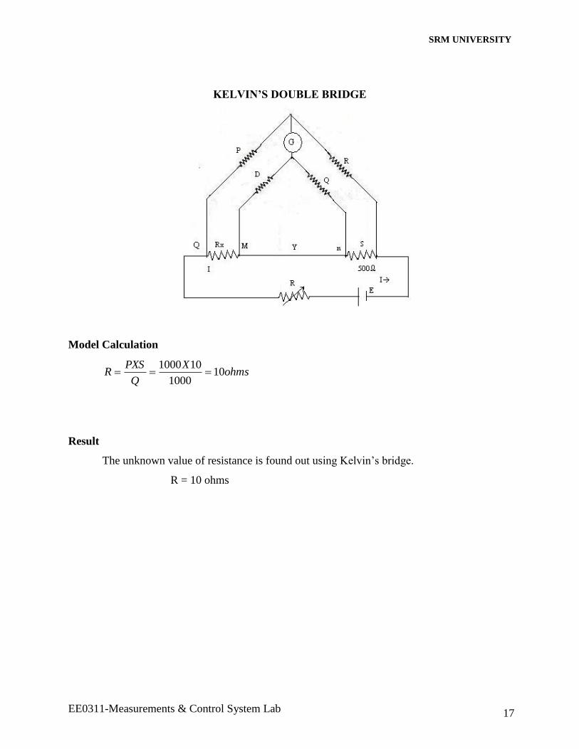
Theory
It is a modification of Wheatstone bridge. In the figure P and Q are the first set of ratio
arms. P and Q are the second set of ratio arms and is used to connect the galvanometer to a point
d at the appropriate potential between points m and n to eliminate the effect of connecting lead of
resistance r between the resistance Rx and the standard resistance S. The ratio p/q is made equal
to P/Q. Under balanced conditions there is no current through the galvanometer.
Eab = Eand
Eab = acEQP
P
and
)(
)(
rqp
rqpSIRE xac
And
)( rqp
prIRE xand
When Eab = Eand
q
p
Q
P
rqp
qr
Q
SRRx
If P/Q = p/q, then Q
SPRx
.
SRM UNIVERSITY
EE0311-Measurements & Control System Lab 16
Formula Used
Unknown resistane of Kelvin’s double bridge
R = PS / Q in ohms
Procedure
The trainer is energized and the power supply +5V is checked
A Galvanometer is connected externally to the trainer.
The unknown resistance ‘R’ is connected in the trainer.
The value of P/Q = p/q = 0.1 ratio
The value of S is adjusted for proper balance and the value of ‘S’ is noted and R is
calculated from the formula
Unknown resistance = R = PS / Q in
Tabulation
Sr.
No.
P Q S Measured
value
R=P S/Q
Set value Rx
Unit K K Ohms Ohms
1 1 1 10 10 10
2 1 1 10 90 100
P, Q : First set of ratio arm
p , q : Second set of ratio arm
Rx : Unknown resistance
S : Standard resistance
R : Resistance of connecting lead
G : Galvanometer
E : Internal Battery
SRM UNIVERSITY
EE0311-Measurements & Control System Lab 17
KELVIN’S DOUBLE BRIDGE
Model Calculation
ohmsX
Q
PXSR 10
1000
101000
Result
The unknown value of resistance is found out using Kelvin’s bridge.
R = 10 ohms
SRM UNIVERSITY
EE0311-Measurements & Control System Lab 18
CALIBRATION OF ENERGY METER ; 1-PHASE
Aim
To calibrate a single phase energy meter by
(i) Direct loading
Apparatus Required
Sl.No. Apparatus Range Quantity
1 Wattmeter 230V, 5A UPF 1
2 Energy meter
3 Voltmeter 0-230V 1
4 Ammeter 0-10A 1
5 Resistive load 10 A 1
Precautions
At the time of switching on the supply, no load must be included
DPST switch is kept open at the time of starting
Procedure
Connection are made as the circuit diagram
By observing the precaution, both the current coils and the pressure coil are supplied
with the rated voltage – in this case 230V.
Now the load is applied gradually till the rated current
All the meter reading are noted down.
SRM UNIVERSITY
EE0311-Measurements & Control System Lab 19
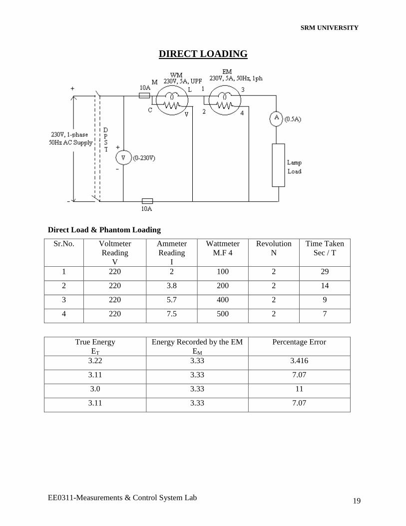
DIRECT LOADING
Direct Load & Phantom Loading
Sr.No. Voltmeter
Reading
V
Ammeter
Reading
I
Wattmeter
M.F 4
Revolution
N
Time Taken
Sec / T
1 220 2 100 2 29
2 220 3.8 200 2 14
3 220 5.7 400 2 9
4 220 7.5 500 2 7
True Energy
ET
Energy Recorded by the EM
EM
Percentage Error
3.22 3.33 3.416
3.11 3.33 7.07
3.0 3.33 11
3.11 3.33 7.07

SRM UNIVERSITY
EE0311-Measurements & Control System Lab 20
Calculation
Power measured by wattmeter is P = Wattmeter read x multiplication fator
True Energy, ET = P x t . . . . wh
Energy recorded by the energy mete is
EM = energy meter constant x N . . . . . .Wh
Percentage Error = (EM – ET) x 100%
Result
Thus the single phase energy meter was calibrated by Direct Load
SRM UNIVERSITY
EE0311-Measurements & Control System Lab 21
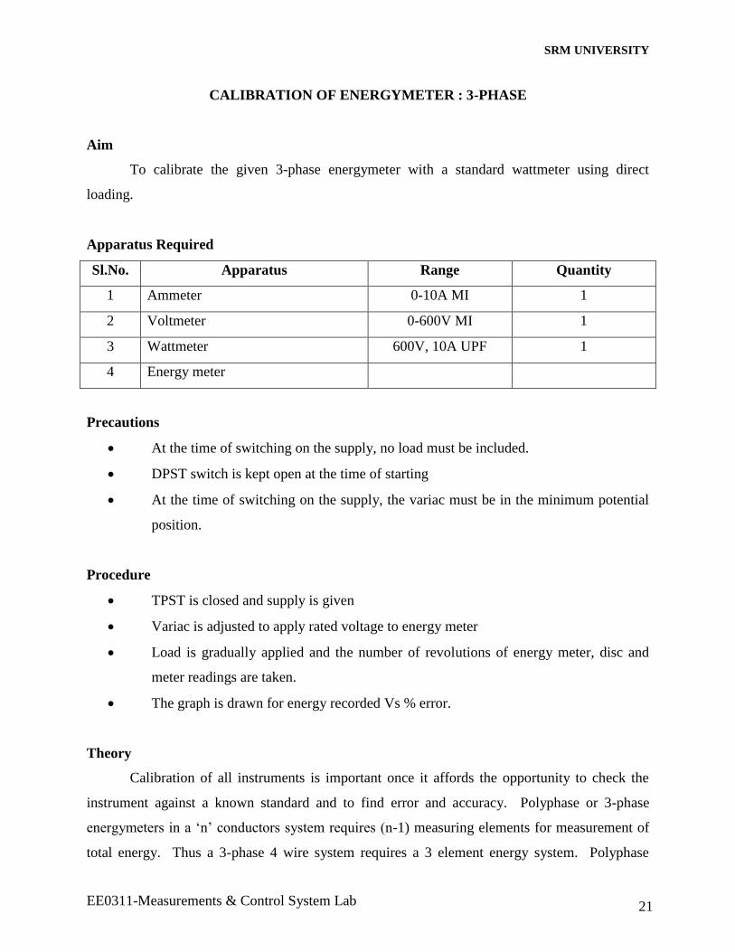
CALIBRATION OF ENERGYMETER : 3-PHASE
Aim
To calibrate the given 3-phase energymeter with a standard wattmeter using direct
loading.
Apparatus Required
Sl.No. Apparatus Range Quantity
1 Ammeter 0-10A MI 1
2 Voltmeter 0-600V MI 1
3 Wattmeter 600V, 10A UPF 1
4 Energy meter
Precautions
At the time of switching on the supply, no load must be included.
DPST switch is kept open at the time of starting
At the time of switching on the supply, the variac must be in the minimum potential
position.
Procedure
TPST is closed and supply is given
Variac is adjusted to apply rated voltage to energy meter
Load is gradually applied and the number of revolutions of energy meter, disc and
meter readings are taken.
The graph is drawn for energy recorded Vs % error.
Theory
Calibration of all instruments is important once it affords the opportunity to check the
instrument against a known standard and to find error and accuracy. Polyphase or 3-phase
energymeters in a ‘n’ conductors system requires (n-1) measuring elements for measurement of
total energy. Thus a 3-phase 4 wire system requires a 3 element energy system. Polyphase
SRM UNIVERSITY
EE0311-Measurements & Control System Lab 22
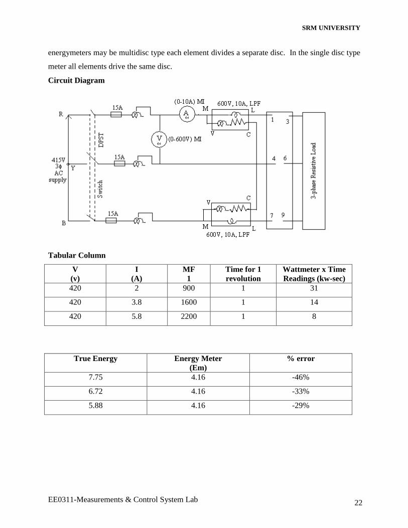
energymeters may be multidisc type each element divides a separate disc. In the single disc type
meter all elements drive the same disc.
Circuit Diagram
Tabular Column
V
(v)
I
(A)
MF
1
Time for 1
revolution
Wattmeter x Time
Readings (kw-sec)
420 2 900 1 31
420 3.8 1600 1 14
420 5.8 2200 1 8
True Energy Energy Meter
(Em)
% error
7.75 4.16 -46%
6.72 4.16 -33%
5.88 4.16 -29%

SRM UNIVERSITY
EE0311-Measurements & Control System Lab 23
Calculation
Power measured by wattmeter is P = wattmeter read x multiplication factor
True Energy, ET = P x t . . . . wh
Energy recorded by the energy mete is
EM = energy meter constant x N . . . . . .Wh
Percentage Error = (EM – ET) x 100%
Result
Hence given 3-phase energy meter was calibrated.
SRM UNIVERSITY
EE0311-Measurements & Control System Lab 24
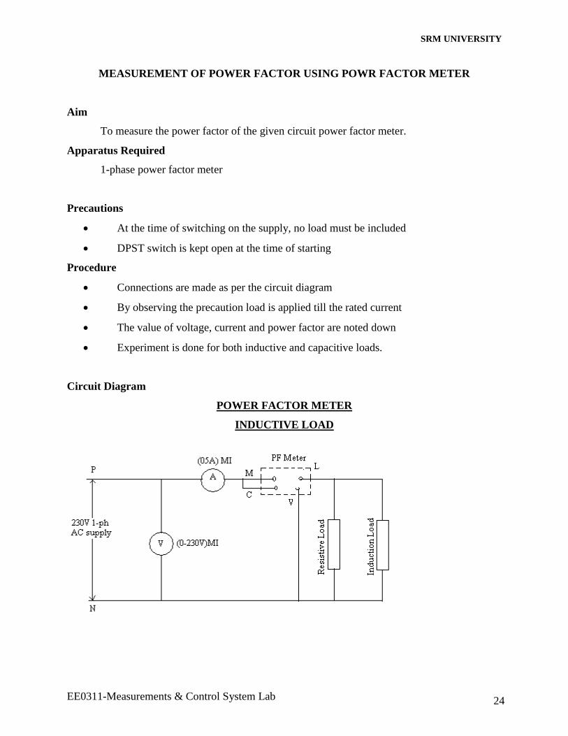
MEASUREMENT OF POWER FACTOR USING POWR FACTOR METER
Aim
To measure the power factor of the given circuit power factor meter.
Apparatus Required
1-phase power factor meter
Precautions
At the time of switching on the supply, no load must be included
DPST switch is kept open at the time of starting
Procedure
Connections are made as per the circuit diagram
By observing the precaution load is applied till the rated current
The value of voltage, current and power factor are noted down
Experiment is done for both inductive and capacitive loads.
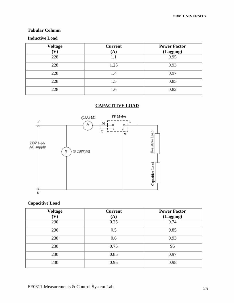
Circuit Diagram
POWER FACTOR METER
INDUCTIVE LOAD
SRM UNIVERSITY
EE0311-Measurements & Control System Lab 25
Tabular Column
Inductive Load
Voltage
(V)
Current
(A)
Power Factor
(Lagging)
228 1.1 0.95
228 1.25 0.93
228 1.4 0.97
228 1.5 0.85
228 1.6 0.82
CAPACITIVE LOAD
Capacitive Load
Voltage
(V)
Current
(A)
Power Factor
(Lagging)
230 0.25 0.74
230 0.5 0.85
230 0.6 0.93
230 0.75 95
230 0.85 0.97
230 0.95 0.98
SRM UNIVERSITY
EE0311-Measurements & Control System Lab 26
SRM UNIVERSITY
EE0311-Measurements & Control System Lab 27
SYNCHRO TRANSMITTER & RECEIVER PAIR
A synchro is an electromagnetic transducer commonly used to convert an angular
position of a shaft into an electric signal.
The basic synchro is usually called a synchro transmitter. Its construction is similar to
that of a three phase alternator. The stator (stationary member) is of laminated silicon steel and
is slotted to accommodate a balanced three phase winding which is usually of concentric coil
type (Three identical coils are placed n the stator with their axis 120 degree apart) and is Y
connected. The rotor is a dumb bell construction and wound with a concentric coil. An AC
voltage is applied to the rotor winding through slip rings. Ref. Fig. No.1A.
Let an AC voltage Vr (t) = Vr sin Wct … (1) be supplied to the rotor of the synchro
transmitter. Thisvoltage causes a flow of magnetizing current in the rotor coil which produces a
sinusoidally time varying flux directed along its axis and distributed nearly sinusoidal, in the air
gap along stator periphery. Because of transformer action, voltages are induced in each of the
stator coils. As the air gap flux is sinusoidally distributed, the flux linking any stator coil is
proportional to the cosine of the angle between rotor and stator coil axis and so is the voltage
induced in each stator coil.
The stator coil voltages are of course in time phase with each other. Thus we see that the
synchro transmitter (TX) acts like single phase transformer in which rotor coil is the primary and
the stator coils form three secondaries.
Let Vs1 N, Vs2 N and Vs3 respectively be the voltages induced in the stator coils S1, S2
and S3 with respect to the neutral. Then for the rotor position of the synchro transistor shown in
fig.No.1 where the rotor axis makes an angle 0 with the axis of the stator coil S2.
Let Vs1N = KVr sin Wct cos (0+120) (2)
Vs2N = KVr sin Wct cos (0) (3)
Vs3N = KVr sin Wct cos (0+240) (4)
SRM UNIVERSITY
EE0311-Measurements & Control System Lab 28
The three terminal voltages of the stator are
Vs1s2 = Vs1N – Vs2N
= 3 KVr sin (0=240) sin Wct (5)
Vs2S3 = Vs2N – Vs3N
= 3 KVr sin (0+120) sin Wct (6)
= 3 KVr sin (0) sin Wct (7)
When 0 is zero from equation (2) and (3) it is seen that maximum voltage is induced in the stator
coil s2 while it follows from equation (7) that the terminal voltage Vs3s1 is zero. This position
of rotor is defined as the electrical zero of the Tx and is used as a reference for specifying the
angular position of the rotor.
Thus it is seen that the input to the synchro transmitter is the angular position of its rotor
shaft and the output is a set of three single phase voltages given by equation (5), (6) and (7). The
magnitudes of these voltage are functions of a shaft position.
The classical synchro systems consists of two units.
1. Synchro transmitter (Tx)
2. Synchro rceiver (Tr)
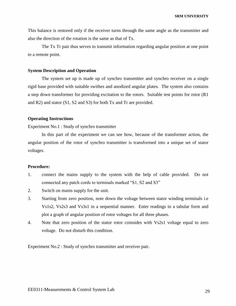
The synchro receiver is having almost the same constructional features. The two units
are connected as shown in figure No.2. Initially the winding S2 of te stator of transmitter is
positioned for maximum coupling with rotor winding. Suppose its voltage is V. The coupling
between S1 and S2 of the stator and primary (Rotor) winding is a cosine function. Therefore the
effective voltages in these winding are proportional to cos 60 degrees or they are V/2 each. So
long as the rotors of the transmitters and receivers remain in this position, no current will flow
between windings because of voltage balance.
When the rotor of Tx is moved to a new position, the voltage balance is disturbed.
Assume that the rotor of Tx is moved through 30 degrees, the stator winding voltages will be
changed to zero, 0.866V and 0.866V respectively. Thus there is a voltage imbalance between
the windings causes currents to 1 flow through the close circuit producing torque that tends to
rotate the rotor of the receiver to a new position where the voltage balance is again restored.
SRM UNIVERSITY
EE0311-Measurements & Control System Lab 29
This balance is restored only if the receiver turns through the same angle as the transmitter and
also the direction of the rotation is the same as that of Tx.
The Tx Tr pair thus serves to transmit information regarding angular position at one point
to a remote point.
System Description and Operation
The system set up is made up of synchro transmitter and synchro receiver on a single
rigid base provided with suitable swithes and anodized angular plates. The system also contains
a step down transformer for providing excitation to the rotors. Suitable test points for rotor (R1
and R2) and stator (S1, S2 and S3) for both Tx and Tr are provided.
Operating Instructions
Experiment No.1 : Study of synchro transmitter
In this part of the experiment we can see how, because of the transformer action, the
angular position of the rotor of synchro transmitter is transformed into a unique set of stator
voltages.
Procedure:
1. connect the mains supply to the system with the help of cable provided. Do not
connected any patch cords to terminals marked “S1, S2 and S3”
2. Switch on mains supply for the unit.
3. Starting from zero position, note down the voltage between stator winding terminals i.e
Vs1s2, Vs2s3 and Vs3s1 in a sequential manner. Enter readings in a tabular form and
plot a graph of angular position of rotor voltages for all three phases.
4. Note that zero position of the stator rotor coinsides with Vs2s1 voltage equal to zero
voltage. Do not disturb this condition.
Experiment No.2 : Study of synchro transmitter and receiver pair.
SRM UNIVERSITY
EE0311-Measurements & Control System Lab 30
Procedure
1. Connect mains supply cable.
2. Connect S1, S2 and S3 terminals of transmitter to S1, S2 and S3 of synchro receiver by
patch cords provided respectively.
3. Switch on SW1 and SW2 and also switch on the mains supply.
SRM UNIVERSITY
EE0311-Measurements & Control System Lab 31
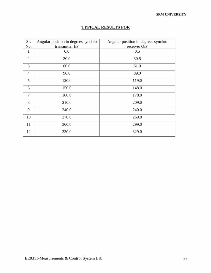
4. Move the pointer i.e rotor position of synchrono transmitter Tx in steps of 30 degrees and
observe the new rotor position. Observe that whenever Tx rotor is rotated, the Tr rotor
follows it for both the directions of rotations and their positions are in good agreement.
5. Enter the input angular position and output angular position in the tabular form and plot a
graph.
Precautions
1. Handle the pointers for both the rotors in a gentle manner
2. Do not attempt to pull out the pointers
3. Do not short rotor or stator terminals
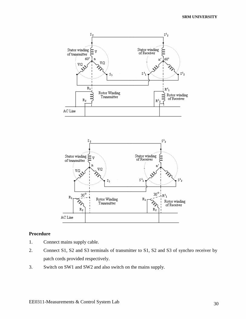
FRONT PANEL VIEW OF SYNCHRO TX AND TR
Note: 1) Connect S1, S2, S3 of synchro transmitter to S1, S2, S3 of synchro receiver
respectively by mans of patch cords.
2) SW1 & SW2 are switches for rotor supply (excitation) of synchro TX &
TR.
SRM UNIVERSITY
EE0311-Measurements & Control System Lab 32
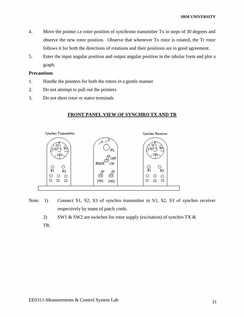
TOP VIEW OF SYNCHRO TRANSMITTER & RECEIVER
SYNCHRO TRANSMITTER ROTOR POSITION VERSUS STATOR VOLTAGES FOR
THREE PHASES
(Vsls3, Vsls2, VS2S3)
Sr.No. Position rotor
degrees
Stator / Vs3S1 Terminal VS1S2 Voltages (RMS)
VS2S3
1 00 0.1 60.3 59.8
2 30 33.8 34.5 68.6
3 60 58.9 1.1 60.7
4 90 69.1 33.7 34.9
5 120 60.1 59.1 0.4
6 150 36.2 68.9 32.6
7 180 0.9 60.3 59.3
8 210 33.9 34.8 68.9
9 240 59.1 0.3 59.6
10 270 68.8 33.5 34.9
11 300 59.7 60 0.4
12 330 33.5 69.2 35.1
SRM UNIVERSITY
EE0311-Measurements & Control System Lab 33
TYPICAL RESULTS FOR
Sr.
No.
Angular position in degrees synchro
transmitter I/P
Angular position in degrees synchro
receiver O/P
1 0.0 0.5
2 30.0 30.5
3 60.0 61.0
4 90.0 89.0
5 120.0 119.0
6 150.0 148.0
7 180.0 178.0
8 210.0 209.0
9 240.0 240.0
10 270.0 269.0
11 300.0 299.0
12 330.0 329.0
SRM UNIVERSITY
EE0311-Measurements & Control System Lab 34
SPEED TORQUE CHARACTERISTICS OF AC SERVO MOTOR
Introduction
An AC servo motor is basically a two phase induction motor except for certain special
design feature. A two phase induction motor consisting of two stator windings oriented 90
degrees electrically apart in space and excited by ac voltage which magnitude and 90 degrees.
Generally voltages of equal magnitude and 90 degrees phase difference are applied to the two
stator phases thus making their respective fields 90 degrees apart in both time and space, at
synchronous speed. As the field sweeps over the rotor, voltages are induced in it producing
current in the short circuited rotor. The rotating magnetic field interacts with these currents
producing a torque on the rotor in the direction of field rotation.
The shape of the characteristics depends upon ratio of the rotor reactance (X) to the rotor
resistance (R). In normal induction motors X/R ratio is generally kept high so as to obtain the
maximum torque close to the operating region which is usually around 5% slip.
A two phase servo motor differs in two ways from normal induction motor.
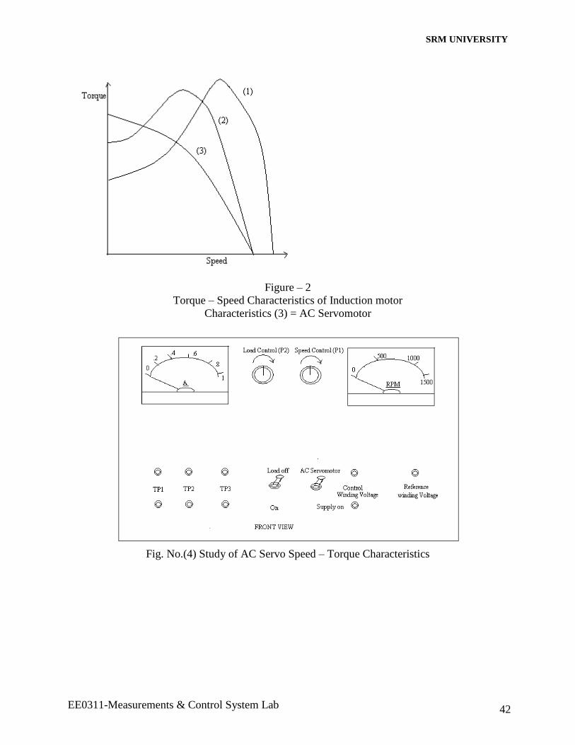
1. The rotor of the servo motor is built with high resistance so that its X/R ratio is small and
the torque speed characteristics is as shown in the figure (2).
Curve (3) is nearly linear in contrast to highly non linear characteristics with large X/R.
It must emphasized that if a conventional induction motor with high X/R ratio is used for
servo applications, then because of the positive slope for part of the characteristics, the
system using such a motor becomes unstable.
The motor construction is usually squirrel cage or drag cup type. The diameter of the
rotor is kept small in order to reduce intertia and thus to obtain good accelerating
characteristics. Drag cup construction is used for a very low intertia operations.
SRM UNIVERSITY
EE0311-Measurements & Control System Lab 35
2. In servo applications, the voltages applied to the two stator windings are seldom
balanced. On of the phases known as the phase known as the control phase with respect
to the voltage supplied to the reference windings and it has a variable magnitude and
polarity. (fig.2). The control winding voltage is supplied from a servo amplifier. For low
power applications, AC servo motors are preferred because they are light weight, rugged
and there are no brush contacts to maintain.
Description of the set up
The motors which is required to be tested is mounted on a small but sturdy pedestal. The
motor is having extension of shafts on both the sides.
Speed variation and speed measurement
The reference winding of the motor is excited from a fixed voltage of 100 volts. The
control winding voltage is obtained through an R-C combination. The voltage available to
control winding is varied by the control of resistance R. The capacitance is used to generate a
phase shift. By varying the magnitude of the control voltage, it is possible to vary the speed of
the AC servo motor. The secondary of the transformer T1 provided the reference winding and
control winding voltage.
On one of the sides of the shaft, a metallic disk with 20 holes (1/4” dia) is mounted. A
photo transistor and light source arrangement is located on the two sides of the disc; so that the
light beam is regularly interrupted by the hole – No- hole arrangement of the disc. The photo
transistor conducts when light is incident on it and acts almost as an open circuit when no light is
falling on it.
In the process the cct generates a train of pulses. The number of pulses per second is
directly proportional to the revolutions persecond. It means for 1500 RPM disc speed, the disc
would be completing 25 revolutions per second and with 20 holes on the disc, 500 pulses would
be generated by the photo pick up in the second. Thus for a sped of 750 rpm, 250 pulses would
be developed by the photo pick up. These pulses are wave shaped by amplifier and a Schmitt
trigger cct. Finally they are fed to a monostable cct which produces constant width and constant
height pulses. Consequently the meter deflection is proportional to the number of pulses per
SRM UNIVERSITY
EE0311-Measurements & Control System Lab 36
second and hence to the rpm of the motor under test. There is a preset in services with the meter
which works as a calibrating control.
A full wave output of a rectifier produces a fixed frequency of 100Hz (within + or – 1%
accuracy) and the same is used as a standard frequency for effecting calibration on the speed
indication. The preset marked “PR1” is to be adjusted for 20% of F.S.D or to 300 rpm. The
switch SW4 is thrown back to normal mode after carrying out calibration check up.
Torque Measurement
In order to measure torque produced by the AC servo motor, we must have an
arrangement to produce a variable load on the AC servo motor. The ac servomotor is
mechanically coupled to a small dc machine (a permanent magnet dc motor or generator) on the
remaining side of the extended shaft. A variable dc current is required to be passed on through
the dc motor. The polarity of the current is such as to produce an opposite torque as a result of
its interaction with the field of the permanent magnet.
In can be proved that the electrical power developed by the AC servo motor is given by
the product of back emf generated by the dc machine and current we are forcing through the
armature by means of a variable resistance and the constant voltage source. By varying the
resistance, the current is changing and the opposite torque is also changing. We have to use the
following formula to find the torque in gm-cm.
cmgmNpi
pT
2
6010019.1 4
where Eb = Back E.M.F
Ia = Armature current
When P = power in watts
= Eb x Ia
N = R.P.M
It P is in milliwatt, proper substitution must be made in the result.
In this formula, Eb can be found by measuring the generated emf across the armature
terminal for a given speed. As the field is constant the output emf (hence back emf) is
proportional to the shaft speed, with armature circuit open circuited, we can run the machine as a
dc generator and find slope (volt/rpm) for the given dc machine.
SRM UNIVERSITY
EE0311-Measurements & Control System Lab 37
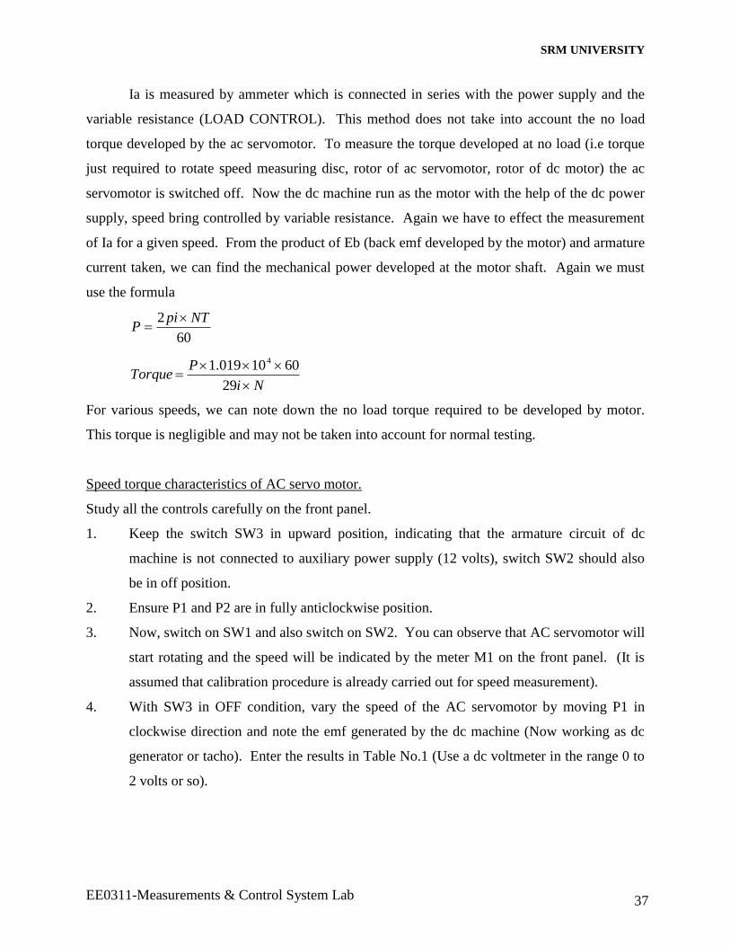
Ia is measured by ammeter which is connected in series with the power supply and the
variable resistance (LOAD CONTROL). This method does not take into account the no load
torque developed by the ac servomotor. To measure the torque developed at no load (i.e torque
just required to rotate speed measuring disc, rotor of ac servomotor, rotor of dc motor) the ac
servomotor is switched off. Now the dc machine run as the motor with the help of the dc power
supply, speed bring controlled by variable resistance. Again we have to effect the measurement
of Ia for a given speed. From the product of Eb (back emf developed by the motor) and armature
current taken, we can find the mechanical power developed at the motor shaft. Again we must
use the formula
60
2 NTpiP
Ni
PTorque
29
6010019.1 4
For various speeds, we can note down the no load torque required to be developed by motor.
This torque is negligible and may not be taken into account for normal testing.
Speed torque characteristics of AC servo motor.
Study all the controls carefully on the front panel.
1. Keep the switch SW3 in upward position, indicating that the armature circuit of dc
machine is not connected to auxiliary power supply (12 volts), switch SW2 should also
be in off position.
2. Ensure P1 and P2 are in fully anticlockwise position.
3. Now, switch on SW1 and also switch on SW2. You can observe that AC servomotor will
start rotating and the speed will be indicated by the meter M1 on the front panel. (It is
assumed that calibration procedure is already carried out for speed measurement).
4. With SW3 in OFF condition, vary the speed of the AC servomotor by moving P1 in
clockwise direction and note the emf generated by the dc machine (Now working as dc
generator or tacho). Enter the results in Table No.1 (Use a dc voltmeter in the range 0 to
2 volts or so).
SRM UNIVERSITY
EE0311-Measurements & Control System Lab 38
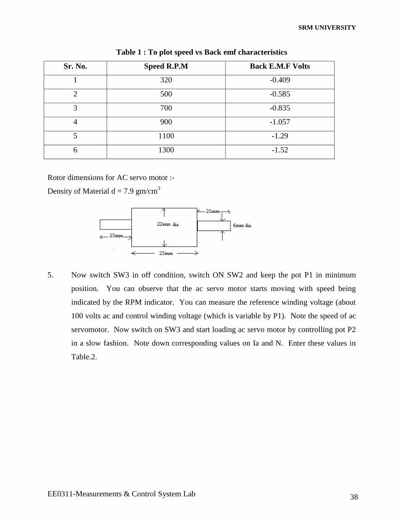
Table 1 : To plot speed vs Back emf characteristics
Sr. No. Speed R.P.M Back E.M.F Volts
1 320 -0.409
2 500 -0.585
3 700 -0.835
4 900 -1.057
5 1100 -1.29
6 1300 -1.52
Rotor dimensions for AC servo motor :-
Density of Material d = 7.9 gm/cm3
5. Now switch SW3 in off condition, switch ON SW2 and keep the pot P1 in minimum
position. You can observe that the ac servo motor starts moving with speed being
indicated by the RPM indicator. You can measure the reference winding voltage (about
100 volts ac and control winding voltage (which is variable by P1). Note the speed of ac
servomotor. Now switch on SW3 and start loading ac servo motor by controlling pot P2
in a slow fashion. Note down corresponding values on Ia and N. Enter these values in
Table.2.
SRM UNIVERSITY
EE0311-Measurements & Control System Lab 39
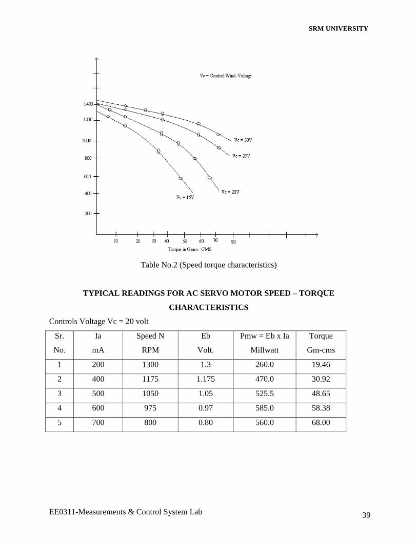
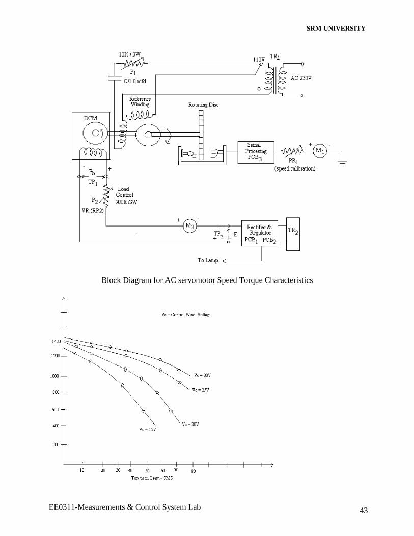
Table No.2 (Speed torque characteristics)
TYPICAL READINGS FOR AC SERVO MOTOR SPEED – TORQUE
CHARACTERISTICS
Controls Voltage Vc = 20 volt
Sr.
No.
Ia
mA
Speed N
RPM
Eb
Volt.
Pmw = Eb x Ia
Millwatt
Torque
Gm-cms
1 200 1300 1.3 260.0 19.46
2 400 1175 1.175 470.0 30.92
3 500 1050 1.05 525.5 48.65
4 600 975 0.97 585.0 58.38
5 700 800 0.80 560.0 68.00
SRM UNIVERSITY
EE0311-Measurements & Control System Lab 40
Controls Voltage Vc = 30 volt
Sr.
No.
Ia
mA
Speed N
RPM
Eb
Volt.
Pmw = Eb x Ia
Millwatt
Torque
Gm-cms
1 200 1400 1.4 280.00 19.46
2 300 1350 1.35 405.00 29.19
3 400 1300 1.3 520.00 38.92
4 600 1200 1.2 720.00 58.38
5 700 1175 1.17 822.5 68.11
Controls Voltage Vc = 40 volt
Sr.
No.
Ia
mA
Speed N
RPM
Eb
Volt.
Pmw = Eb x Ia
Millwatt
Torque
Gm-cms
1 0.05 850 -0.15 -0.0075 -0.858
2 0.15 780 0.66 0.099 12.350
3 0.20 700 1.24 0.248 34.47
4 0.25 620 1.77 0.4425 69.449
5 0.35 550 2.57 0.899 159.053
6. Now you may set control winding voltage to a new value of 30 volts after switching of
SW3. Again repeat the process as indicated in step No.5 i.e. Table 2 for a new value of
control winding voltage.
7. Plot the speed torque characteristics for various values of control winding voltages.
Study their nature.
Precautions
1. Before switch on, P1 and P2 should be always brought to most anticlockwise position.
2. Controls P1 and P2 should be operated in a gentle fashion.
SRM UNIVERSITY
EE0311-Measurements & Control System Lab 41
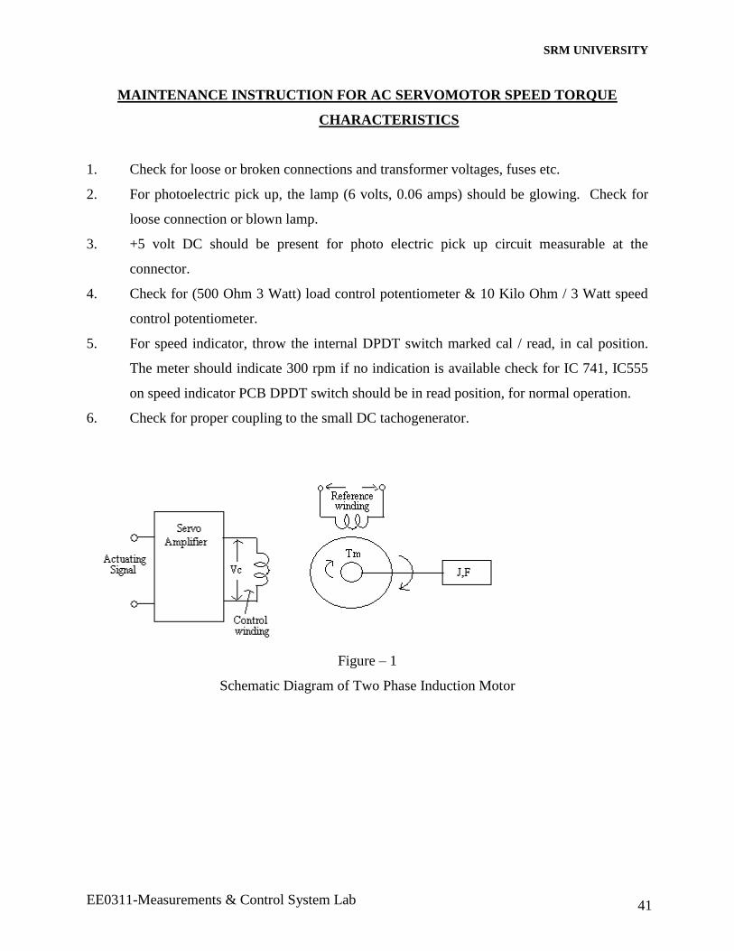
MAINTENANCE INSTRUCTION FOR AC SERVOMOTOR SPEED TORQUE
CHARACTERISTICS
1. Check for loose or broken connections and transformer voltages, fuses etc.
2. For photoelectric pick up, the lamp (6 volts, 0.06 amps) should be glowing. Check for
loose connection or blown lamp.
3. +5 volt DC should be present for photo electric pick up circuit measurable at the
connector.
4. Check for (500 Ohm 3 Watt) load control potentiometer & 10 Kilo Ohm / 3 Watt speed
control potentiometer.
5. For speed indicator, throw the internal DPDT switch marked cal / read, in cal position.
The meter should indicate 300 rpm if no indication is available check for IC 741, IC555
on speed indicator PCB DPDT switch should be in read position, for normal operation.
6. Check for proper coupling to the small DC tachogenerator.
Figure – 1
Schematic Diagram of Two Phase Induction Motor
SRM UNIVERSITY
EE0311-Measurements & Control System Lab 42
Figure – 2
Torque – Speed Characteristics of Induction motor
Characteristics (3) = AC Servomotor
Fig. No.(4) Study of AC Servo Speed – Torque Characteristics
SRM UNIVERSITY
EE0311-Measurements & Control System Lab 43
Block Diagram for AC servomotor Speed Torque Characteristics
SRM UNIVERSITY
EE0311-Measurements & Control System Lab 44
TYPICAL TORQUE CALCULATION OF POINT ‘A’ ON GRAPH 2
EC = 70 volt
Ia = 170 milli Amp. = 0.17 amp.
Speed ‘N’ = 850 RPM
For speed 850 RPM., Eb – 960 milli volt = 0.96 volt
Therefore power ‘p’ = Eb x Ia = 0.96 x 0.17 = 0.1632 watt
Therefore
Npi
pTTorque
2
6010019.1''
4
850142.32
6010019.11632.0''
4
T
T = 18.68 Gm Cm.
Therefore point ‘A’ (18,68,850), which is plotted on graph 2.
ANALYSIS OF AC SERVOMOTOR SPEED-TORQUE CHARACTERISTICS
We observed that the torque – speed curves are not straight lines. Therefore a linear
differential equation cannot be used to represent the exact motor characteristics. Sufficient
accuracy may be obtained by approximating the characteristics by straight lines. The following
analysis is based on this assumption.
(Reference : - feedback control system analysis & synthesis by J.J.D’AZZO & H.Houpis . Page
No.48)
The torque generated is a function of both the speed W & the control winding voltage ec.
In terms of partial derivatives, the torque equation is
SRM UNIVERSITY
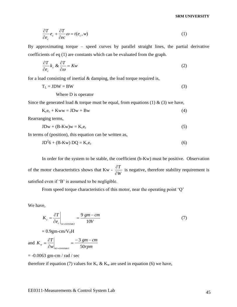
EE0311-Measurements & Control System Lab 45
),( wetec
Te
e
Tcc
c
(1)
By approximating torque – speed curves by parallel straight lines, the partial derivative
coefficients of eq (1) are constants which can be evaluated from the graph.
KwT
ke
Tc
c
& (2)
for a load consisting of inertial & damping, the load torque required is,
TL = JDW = BW (3)
Where D is operator
Since the generated load & torque must be equal, from equations (1) & (3) we have,
Kcec + Kww = JDw + Bw (4)
Rearranging terms,
JDw + (B-Kw)w = Kcec (5)
In terms of (position), this equation can be written as,
JD26 + (B-Kw) DQ = Kcec (6)
In order for the system to be stable, the coefficient (b-Kw) must be positive. Observation
of the motor characteristics shows that Kw - W
T
is negative, therefore stability requirement is
satisfied even if ‘B’ is assumed to be negligible.
From speed torque characteristics of this motor, near the operating point ‘Q’
We have,
V
cmgm
e
TK
tconswc
c10
9
tan
(7)
= 0.9gm-cm/V0H
and rpm
cmgm
w
TK
tconsec
w50
3
tan
= -0.0063 gm-cm / rad / sec
therefore if equation (7) values for Kc & Kw are used in equation (6) we have,

SRM UNIVERSITY
EE0311-Measurements & Control System Lab 46
JD2Q + (B+0.0063) DQ =
V
cmegm c9.0 (8)
Where values for ‘J’ and ‘B’ can be inserted if ‘B’ is negligible, only ‘J’ value need be
introduced.
SRM UNIVERSITY
EE0311-Measurements & Control System Lab 47
TRANSFER FUNCTION OF FIELD CONTROLLED DC MOTOR
Aim
To determine the transfer function of a field controlled DC motor.
Apparatus Required
Sl. No. Apparatus Type & Range Quantity
1 Ammeter (0-10A) MC
(0-2A) MC
(0-2A0 MI
1
1
1
2 Voltmeter (0-300V) MC
(050) MC
1
2
3 Rheostat 300 / 1.2A
100 / 3A
1
1
Formula
The transfer function of a field controlled DC motor is
)}1)(1{()(
)(
mf
m
f STST
K
E
Tm = Mechanical time constant of rotor = J/B
J = Moment of Inertia of rotor = Kg m2 / rad – sec
Lf = Field inductance (H)
Km = Determined Using Load Test
T = R x 9.8 X (S1 ~ S2) N-M
Tf = Time constant of field circuit Lf / Rf
Procedure
I) To determine motor gain constant – Km (Load test):-
1. Motor field rheostat is kept at minimum position
2. Supply is given and the motor is started
3. Adjust the motor field rheostat and bring the motor to rated speed
SRM UNIVERSITY
EE0311-Measurements & Control System Lab 48
4. Voltmeter, ammeter and spring balance readings are noted
5. Readings are taken for different field event keeping armature current cut
II) Retardation Test:-
1. Connections are given as per the circuit diagram
2. Motor sis started on no load
3. Motor field rheostat is adjusted to bring the motor slightly above the rated speed
4. Using DPDT switch supply is cut off and motor is allowed to retard
5. Different values of speed changes to the corresponding time are noted
6. Now motor is started as usual and brought to rated speed
7. DPDT switch is thrown off such that supply to armature is cut off, but a known
resistance R is connected to the armature and the motor is allowed to retard.
8. Time taken of 5% fall in speed, voltmeter voltmeter and current readings are
noted.
9. Similarly time taken for 5% fall in speed without R is obtained.
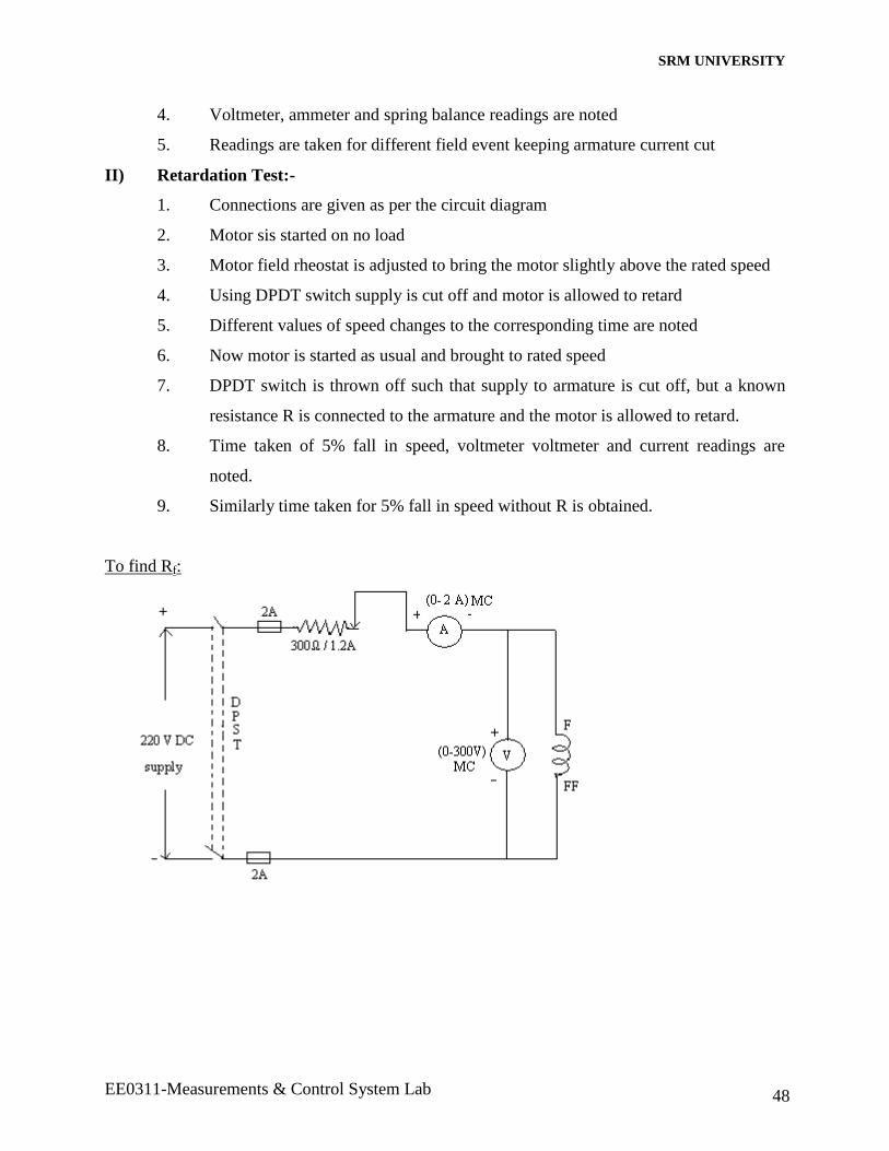
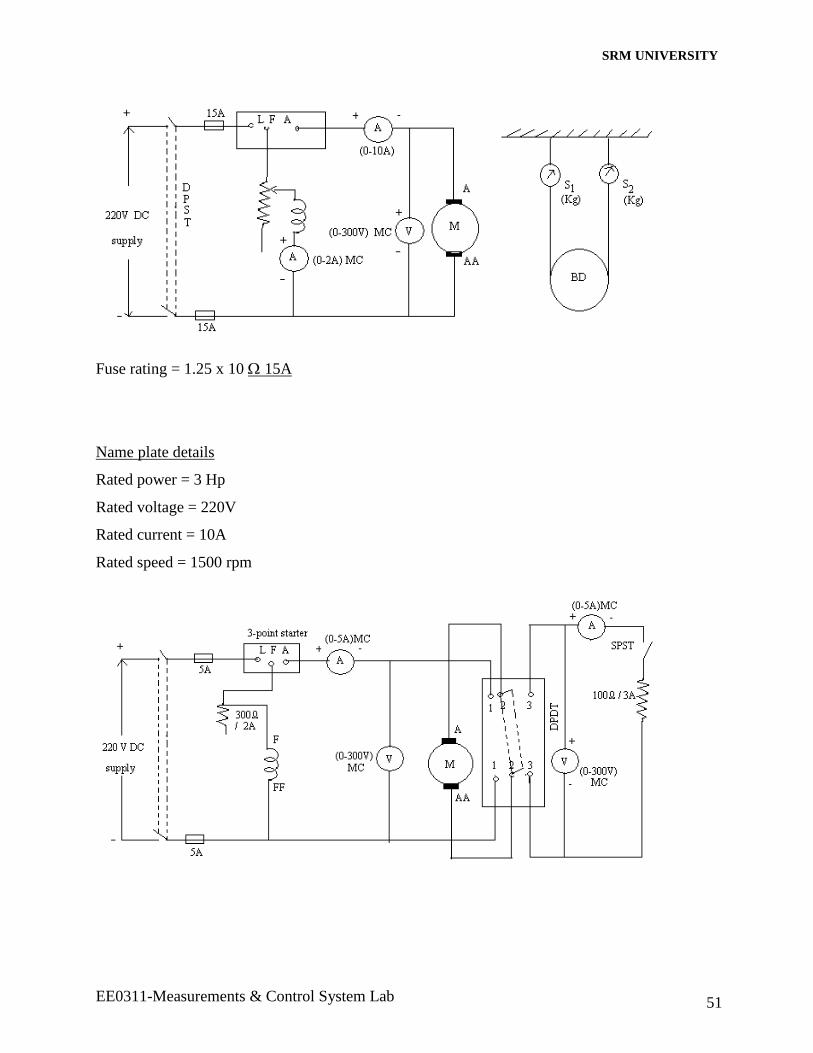
To find Rf:
SRM UNIVERSITY
EE0311-Measurements & Control System Lab 49
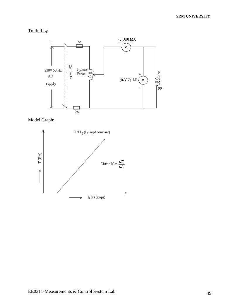
To find Lf:
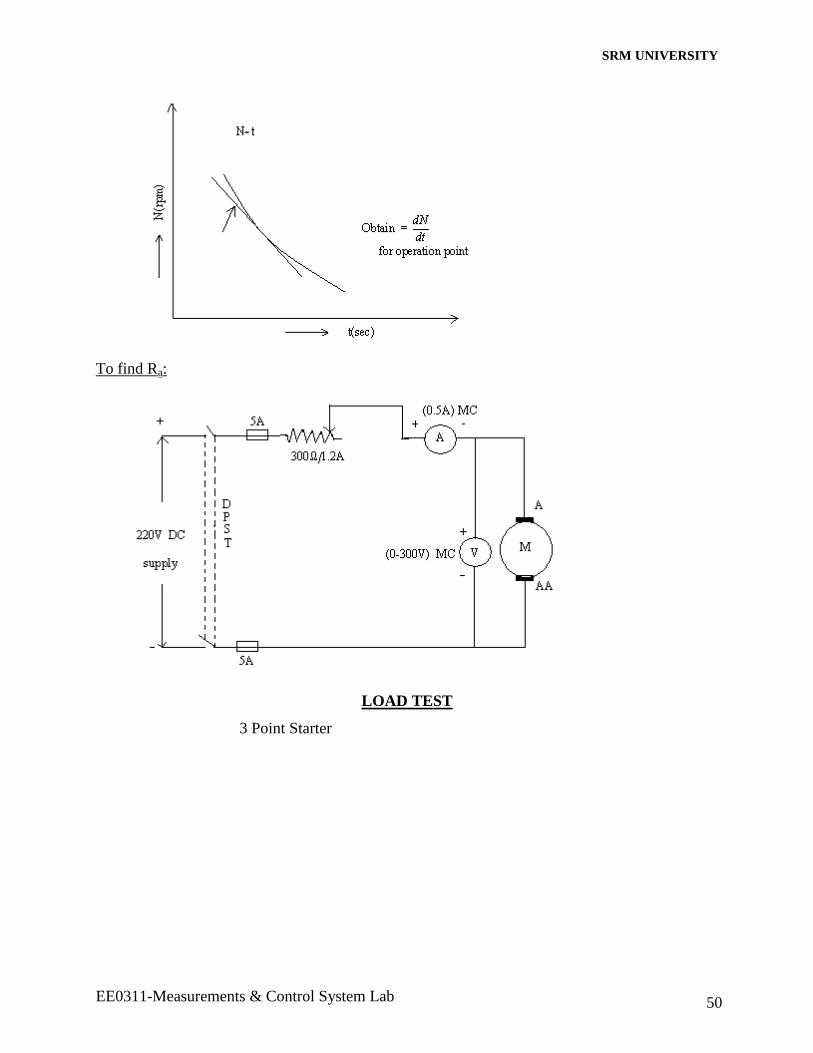
Model Graph:
SRM UNIVERSITY
EE0311-Measurements & Control System Lab 50
To find Ra:
LOAD TEST
3 Point Starter
SRM UNIVERSITY
EE0311-Measurements & Control System Lab 51
Fuse rating = 1.25 x 10 15A
Name plate details
Rated power = 3 Hp
Rated voltage = 220V
Rated current = 10A
Rated speed = 1500 rpm
SRM UNIVERSITY
EE0311-Measurements & Control System Lab 52
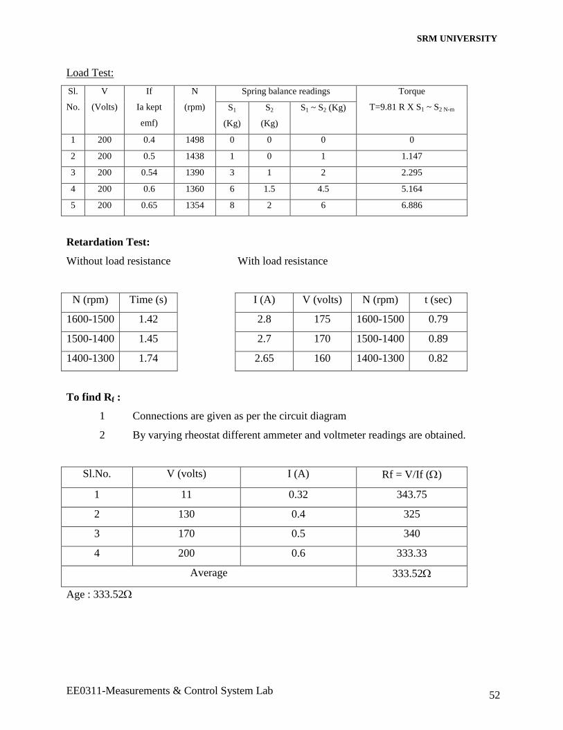
Load Test:
Sl.
No.
V
(Volts)
If
Ia kept
emf)
N
(rpm)
Spring balance readings Torque
T=9.81 R X S1 ~ S2 N-m S1
(Kg)
S2
(Kg)
S1 ~ S2 (Kg)
1 200 0.4 1498 0 0 0 0
2 200 0.5 1438 1 0 1 1.147
3 200 0.54 1390 3 1 2 2.295
4 200 0.6 1360 6 1.5 4.5 5.164
5 200 0.65 1354 8 2 6 6.886
Retardation Test:
Without load resistance With load resistance
N (rpm) Time (s) I (A) V (volts) N (rpm) t (sec)
1600-1500 1.42 2.8 175 1600-1500 0.79
1500-1400 1.45 2.7 170 1500-1400 0.89
1400-1300 1.74 2.65 160 1400-1300 0.82
To find Rf :
1 Connections are given as per the circuit diagram
2 By varying rheostat different ammeter and voltmeter readings are obtained.
Sl.No. V (volts) I (A) Rf = V/If ()
1 11 0.32 343.75
2 130 0.4 325
3 170 0.5 340
4 200 0.6 333.33
Average 333.52
Age : 333.52
SRM UNIVERSITY
EE0311-Measurements & Control System Lab 53
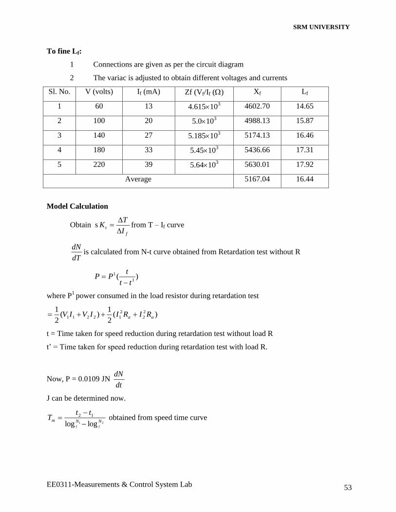
To fine Lf:
1 Connections are given as per the circuit diagram
2 The variac is adjusted to obtain different voltages and currents
Sl. No. V (volts) If (mA) Zf (Vf/If () Xf Lf
1 60 13 4.615103 4602.70 14.65
2 100 20 5.0103 4988.13 15.87
3 140 27 5.185103 5174.13 16.46
4 180 33 5.45103 5436.66 17.31
5 220 39 5.64103 5630.01 17.92
Average 5167.04 16.44
Model Calculation
Obtain sf
tI
TK
from T – If curve
dT
dNis calculated from N-t curve obtained from Retardation test without R
)(1
1
tt
tPP
where P1
power consumed in the load resistor during retardation test
)(2
1)(
2
1 2
2
2
12211 aa RIRIIVIV
t = Time taken for speed reduction during retardation test without load R
t’ = Time taken for speed reduction during retardation test with load R.
Now, P = 0.0109 JN dt
dN
J can be determined now.
21 loglog
12
NNm
ttT
obtained from speed time curve
SRM UNIVERSITY
EE0311-Measurements & Control System Lab 54
Find B = mT
J
BR
KK
f
tm
Substituting the values for different constants in the general formula for TF, we get the transfer
function of the given M/C
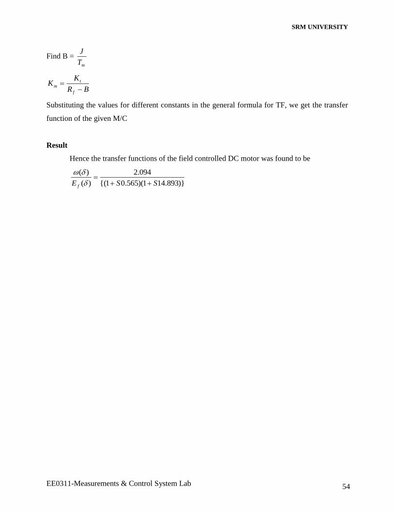
Result
Hence the transfer functions of the field controlled DC motor was found to be
)}893.141)(565.01{(
094.2
)(
)(
SSE f
SRM UNIVERSITY
EE0311-Measurements & Control System Lab 55
TRANSFER FUNCTION OF LAG, LEAD NETWORK
Aim
To obtain the transfer function of a lag, lead network
Apparatus Required
Sl. No. Apparatus Type & Range Quantity
1 Resistor 1K
470
1
1
2 Capacitor 0.1f 1
3 Function Generator -- 1
4 CRO -- 1
Description
Compensation is essentially a compromise between steady state accuracy and relative
stability.
a) Load Compensation: There are many ways to realize continuous time lead
compensators of which one is an electrical RC network. Lead compensators
essentially yields an appreciable improvement in transient response and a small
change in steady state accuracy. It way accentuate high frequency noise effects. A
lead compensator is basically a high pass filter i. high frequencies are passed.
b) Lag Compensation: This yields an appreciable improvement in steady state accuracy
at the expense of increasing the transient response time. It will suppers the effect of
high frequency noise effects. It permits a high gain at low frequencies which
improves steady state performance. In lag compensation we use attenuation
characteristic at high frequencies rather than the phase lag characteristic. Lag
compensation increases the low frequency gain and thus improves the steady
accuracy of the system, but reduced the speed of response due to reduced bandwidth.
Procedure
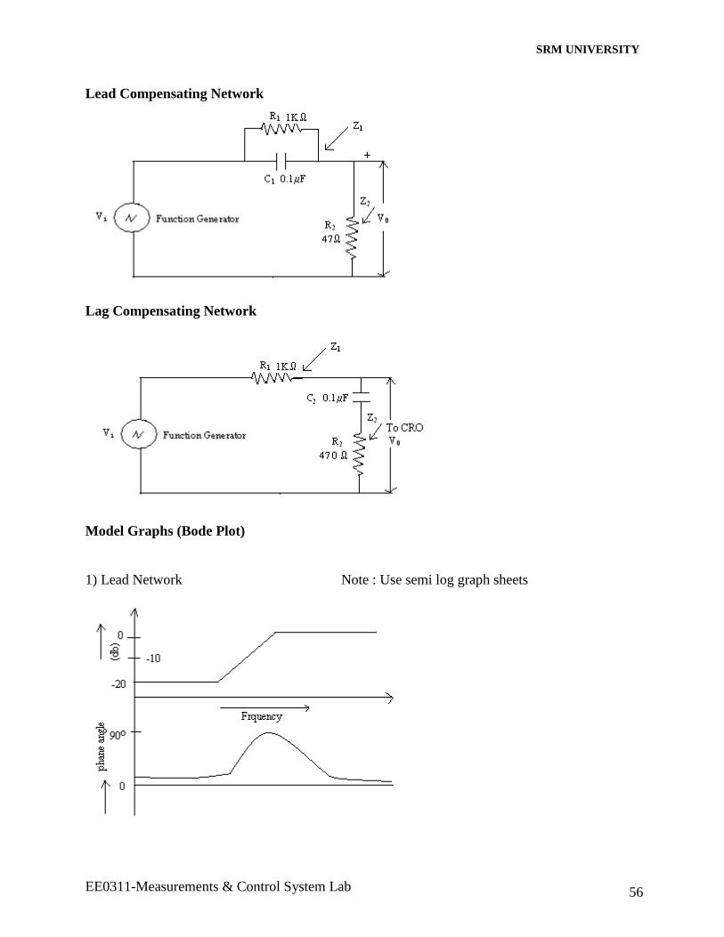
1. The connections are given as per the circuit diagram
2. Using function generator, input is given and the output is observed at the CRO
3. For different values of frequencies, the values of a, b and output voltage are
determined.
4. The graph is drawn by taking frequencies along X-axis and magnitude and phase
along Y-axis.
SRM UNIVERSITY
EE0311-Measurements & Control System Lab 56
Lead Compensating Network
Lag Compensating Network
Model Graphs (Bode Plot)
1) Lead Network Note : Use semi log graph sheets
SRM UNIVERSITY
EE0311-Measurements & Control System Lab 57
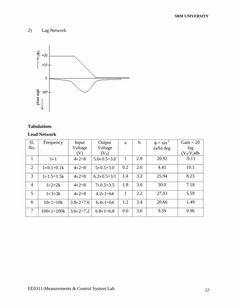
2) Lag Network
Tabulations
Lead Network
Sl.
No.
Frequency Input
Voltage
(V)
Output
Voltage
(V0)
a b = sin-1
(a/b) deg
Gain = 20
log
(V0/Vi)db
1 11 42=8 5.60.5=3.0 1 2.8 20.92 -9.11
2 10.1=0.1k 42=8 50.5=3.0 0.2 2.6 4.41 10.1
3 11.5=1.5k 42=8 6.20.5=3.1 1.4 3.2 25.94 8.23
4 12=2k 42=8 70.5=3.5 1.8 3.6 30.0 7.18
5 13=3k 42=8 4.21=64 1 2.2 27.03 5.59
6 101=10k 3.82=7.6 6.41=64 1.2 3.4 20.66 1.49
7 1001=100k 3.62=7.2 6.81=6.8 0.6 3.6 9.59 0.96
SRM UNIVERSITY
EE0311-Measurements & Control System Lab 58
Lag Network
Sl.
No.
Frequency Input
Voltage
(V)
Output
Voltage
(V0)
a b = sin-1
(a/b) deg
Gain = 20
log
(V0/Vi)db
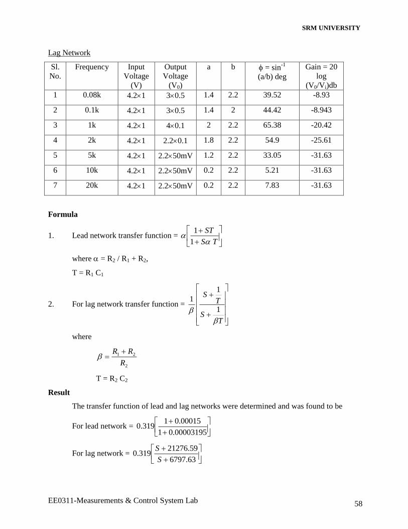
1 0.08k 4.21 30.5 1.4 2.2 39.52 -8.93
2 0.1k 4.21 30.5 1.4 2 44.42 -8.943
3 1k 4.21 40.1 2 2.2 65.38 -20.42
4 2k 4.21 2.20.1 1.8 2.2 54.9 -25.61
5 5k 4.21 2.250mV 1.2 2.2 33.05 -31.63
6 10k 4.21 2.250mV 0.2 2.2 5.21 -31.63
7 20k 4.21 2.250mV 0.2 2.2 7.83 -31.63
Formula
1. Lead network transfer function =
TS
ST
1
1
where = R2 / R1 + R2,
T = R1 C1
2. For lag network transfer function =
TS
TS
1
1
1
where
2
21
R
RR
T = R2 C2
Result
The transfer function of lead and lag networks were determined and was found to be
For lead network =
00003195.01
00015.01319.0
For lag network =
63.6797
59.21276319.0
S
S
SRM UNIVERSITY
EE0311-Measurements & Control System Lab 59
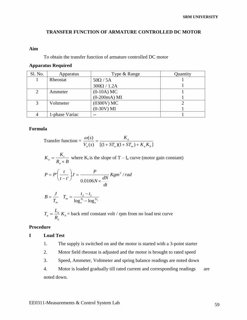
TRANSFER FUNCTION OF ARMATURE CONTROLLED DC MOTOR
Aim
To obtain the transfer function of armature controlled DC motor
Apparatus Required
Sl. No. Apparatus Type & Range Quantity
1 Rheostat 50 / 5A
300 / 1.2A
1
1
2 Ammeter (0-10A) MC
(0-200mA) MI
1
1
3 Voltmeter (0300V) MC
(0-30V) MI
2
1
4 1-phase Variac -- 1
Formula
Transfer function = ])1)(1[()(
)(
bama
a
a KKSTST
K
sV
s
BR
KK
a
t
a
where Kt is the slope of T – Ia curve (motor gain constant)
radKgm
dt
dNN
PJ
tt
tPP /
0106.0
.'
' 2
21 loglog
12
N
e
N
e
m
m
ttT
T
JB
b
a
a
a KR
LT = back emf constant volt / rpm from no load test curve
Procedure
I Load Test
1. The supply is switched on and the motor is started with a 3-point starter
2. Motor field rheostat is adjusted and the motor is brought to rated speed
3. Speed, Ammeter, Voltmeter and spring balance readings are noted down
4. Motor is loaded gradually till rated current and corresponding readings are
noted down.
SRM UNIVERSITY
EE0311-Measurements & Control System Lab 60
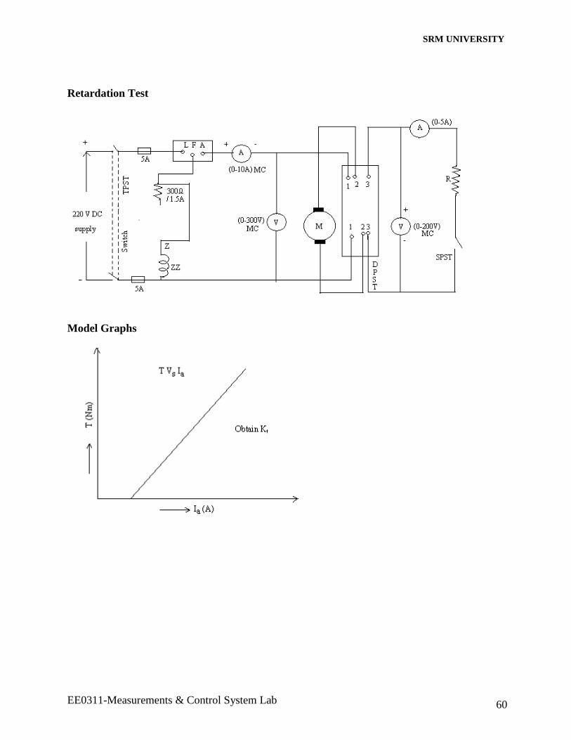
Retardation Test
Model Graphs
SRM UNIVERSITY
EE0311-Measurements & Control System Lab 61
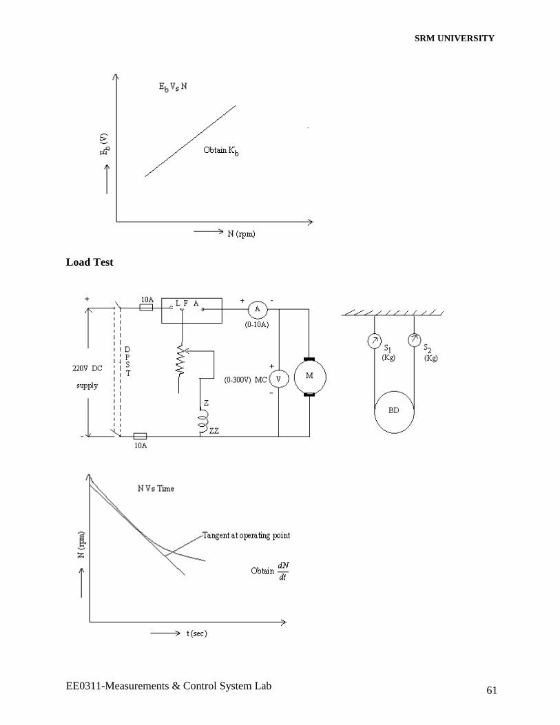
Load Test
SRM UNIVERSITY
EE0311-Measurements & Control System Lab 62
To find Ra
To find La
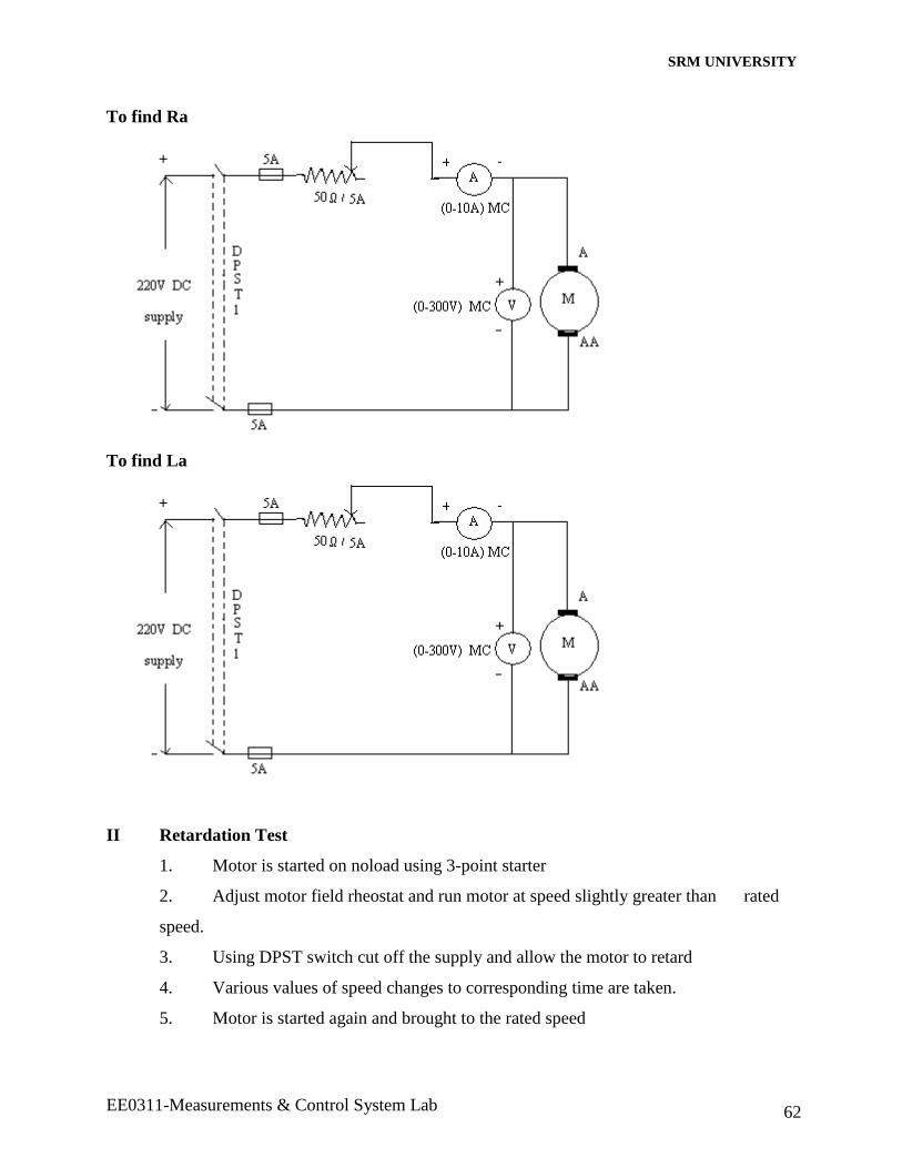
II Retardation Test
1. Motor is started on noload using 3-point starter
2. Adjust motor field rheostat and run motor at speed slightly greater than rated
speed.
3. Using DPST switch cut off the supply and allow the motor to retard
4. Various values of speed changes to corresponding time are taken.
5. Motor is started again and brought to the rated speed
SRM UNIVERSITY
EE0311-Measurements & Control System Lab 63
6. DPST switch is used to cut off armature supply but a known resistance is added
to armature circuit & motor is allowed to retard.
7. Time for 5% fall on speed & corresponding voltmeter, ammeter readings are
noted down.
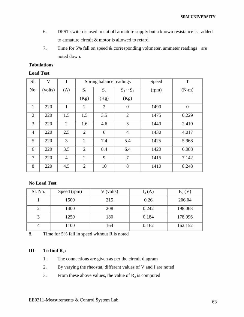
Tabulations
Load Test
Sl.
No.
V
(volts)
I
(A)
Spring balance readings Speed
(rpm)
T
(N-m) S1
(Kg)
S2
(Kg)
S1 ~ S2
(Kg)
1 220 1 2 2 0 1490 0
2 220 1.5 1.5 3.5 2 1475 0.229
3 220 2 1.6 4.6 3 1440 2.410
4 220 2.5 2 6 4 1430 4.017
5 220 3 2 7.4 5.4 1425 5.968
6 220 3.5 2 8.4 6.4 1420 6.088
7 220 4 2 9 7 1415 7.142
8 220 4.5 2 10 8 1410 8.248
No Load Test
Sl. No. Speed (rpm) V (volts) Ia (A) Eb (V)
1 1500 215 0.26 206.04
2 1400 208 0.242 198.068
3 1250 180 0.184 178.096
4 1100 164 0.162 162.152
8. Time for 5% fall in speed without R is noted
III To find Ra:
1. The connections are given as per the circuit diagram
2. By varying the rheostat, different values of V and I are noted
3. From these above values, the value of Ra is computed
SRM UNIVERSITY
EE0311-Measurements & Control System Lab 64
IV To find La:
1. The connections are given as per the circuit diagram
2. By varying the 1 phase variac, different values of V and I are noted
3. From these values, the values of Z are obtained. From Z and Ra, the value of Xa
(and hence La) are computed.
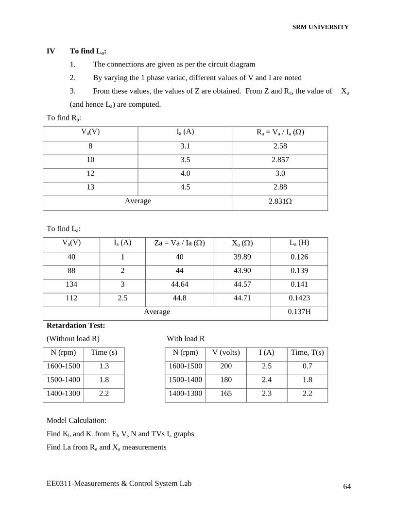
To find Ra:
Va(V) Ia (A) Ra = Va / Ia ()
8 3.1 2.58
10 3.5 2.857
12 4.0 3.0
13 4.5 2.88
Average 2.831
To find La:
Va(V) Ia (A) Za = Va / Ia () Xa () La (H)
40 1 40 39.89 0.126
88 2 44 43.90 0.139
134 3 44.64 44.57 0.141
112 2.5 44.8 44.71 0.1423
Average 0.137H
Retardation Test:
(Without load R) With load R
N (rpm) Time (s) N (rpm) V (volts) I (A) Time, T(s)
1600-1500 1.3 1600-1500 200 2.5 0.7
1500-1400 1.8 1500-1400 180 2.4 1.8
1400-1300 2.2 1400-1300 165 2.3 2.2
Model Calculation:
Find Kb and Kt from Eb Vs N and TVs Ia graphs
Find La from Ra and Xa measurements
SRM UNIVERSITY
EE0311-Measurements & Control System Lab 65
Determine dN / dt, the slope of NVs Time graph
)(2
1)(
2
1' 2
2
2
12211 aa RIRIIVIVP from retardation test values with load
t1 = Time in ‘sec’ for retardation of the machine with resistive load
t = Time in ‘sec’ for retardation of the machine without resistive load
find
dt
dNN
PJ
ttT
NNm
0109.0
,loglog 21
12
wheremT
JB
tt
tPP
''
BR
KK
a
t
a
. Obtain transfer function by substitution of constants.
Result
Hence the transfer function of the given armature controlled DC motor was found to be
}67.5)783.51)(0412.01{(
61.38
)(
)(
SSsR
s
a
SRM UNIVERSITY
EE0311-Measurements & Control System Lab 66
STABILITY ANALYSIS OF LINEAR SYSTEMS
Aim
To analyze the stability of the linear systems using Bode / Root locus / Nyquist plot,
using MATLAB Software tool.
Theory
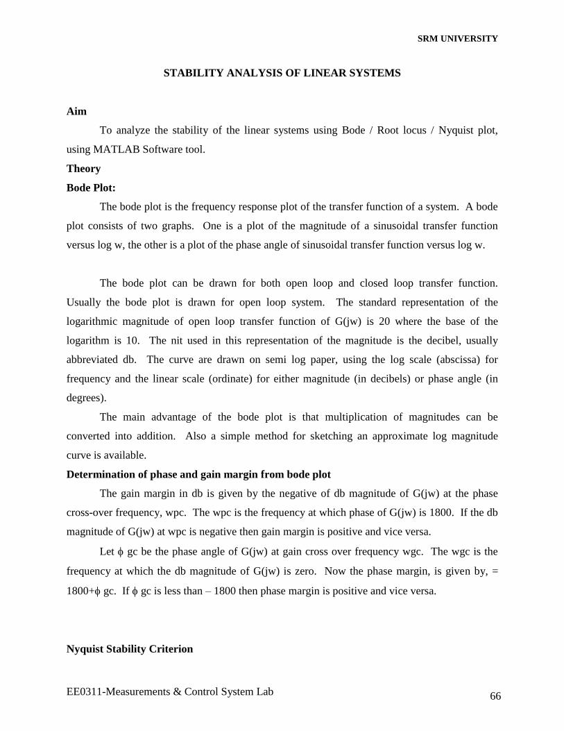
Bode Plot:
The bode plot is the frequency response plot of the transfer function of a system. A bode
plot consists of two graphs. One is a plot of the magnitude of a sinusoidal transfer function
versus log w, the other is a plot of the phase angle of sinusoidal transfer function versus log w.
The bode plot can be drawn for both open loop and closed loop transfer function.
Usually the bode plot is drawn for open loop system. The standard representation of the
logarithmic magnitude of open loop transfer function of G(jw) is 20 where the base of the
logarithm is 10. The nit used in this representation of the magnitude is the decibel, usually
abbreviated db. The curve are drawn on semi log paper, using the log scale (abscissa) for
frequency and the linear scale (ordinate) for either magnitude (in decibels) or phase angle (in
degrees).
The main advantage of the bode plot is that multiplication of magnitudes can be
converted into addition. Also a simple method for sketching an approximate log magnitude
curve is available.
Determination of phase and gain margin from bode plot
The gain margin in db is given by the negative of db magnitude of G(jw) at the phase
cross-over frequency, wpc. The wpc is the frequency at which phase of G(jw) is 1800. If the db
magnitude of G(jw) at wpc is negative then gain margin is positive and vice versa.
Let gc be the phase angle of G(jw) at gain cross over frequency wgc. The wgc is the
frequency at which the db magnitude of G(jw) is zero. Now the phase margin, is given by, =
1800+ gc. If gc is less than – 1800 then phase margin is positive and vice versa.
Nyquist Stability Criterion
SRM UNIVERSITY
EE0311-Measurements & Control System Lab 67
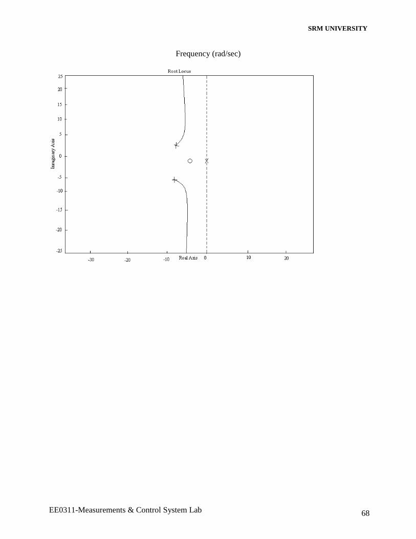
If the G(S) H(S) contour in the G(S) H(S) plane corresponding to Nyquist contour in the
s-plane encircles the point (-1+j0) in the anticlockwise direction as many times as the number of
halfs-plan poles of G(S) H(S), then the closed loop system is stable.
In examining the stability of linear control systems using the Nyquist stability criterion,
the following three situations.
1. There is no encirclement of -1+j0 point. This implies that the system is stable if there are
no poles of G(S) H(S) in the right half s-plan. If there are poles on right half s-plane then
the system is unstable.
Bode Diagram
SRM UNIVERSITY
EE0311-Measurements & Control System Lab 68
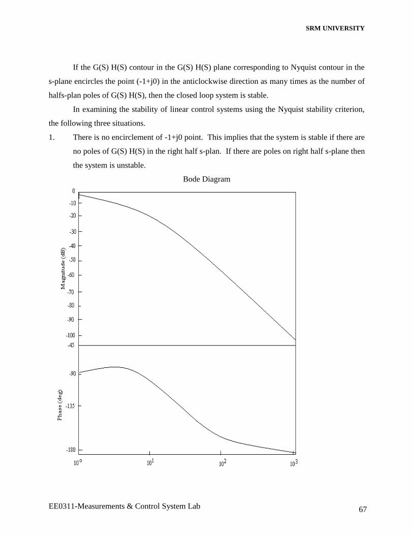
Frequency (rad/sec)
SRM UNIVERSITY
EE0311-Measurements & Control System Lab 69
2. An anticlowise encirclement or (or encirclements) of -1+j0 point. In this case the system
is stable if the number of anticlociwise encirclement is same as the number of poles of
G(S) H(S) in the right half s-plane. If the number of encirclement is not equal to number
of poles on right half s-plane then the system is unstable.
3. There is a clockwise encirclement (or encirclement) of the -1+j0 point. In this case the
system is always unstable.
Procedure
1. Write programs for the given transfer function
2. Simulate it using MATLAB software
3. Observe the graph
4. Calculate the theoretical values for the time domain specifications and compare with the
observed values.

SRM UNIVERSITY
EE0311-Measurements & Control System Lab 70
Programme & Plots
%Root locus;
% G is the transfer function
s=tf(‘s’)
G=75*(1+0.2*s)/(s*(s^s+16*s+100));
rlocus(G);
axis equal;
% Nyquist plot
s=tf(‘s’);
G=75*(1+0.2*s)/(s*(s^s+16*s+100));
nyquist(G);
axis equal;
% Bode plot
s=tf(‘s’);
G=75*(1+0.2*s)/(s*(s^s+16*s+100));
bode(G);
axis equal;
Result
The response of the given transfer using Bode plot, Nyquist Plot & Root locus obtained
using the MATLAB. The theoretical values and practical values are compared.


![BT 0502 - M.Tech r-DNA Technology lab manual[1]webstor.srmist.edu.in/web_assets/srm_mainsite/files... · enzyme has a specific restriction site at which it cuts a DNA molecule. For](https://img.pdfslide.net/doc/110x75/5e4d1c525de91f77ce488c04/bt-0502-mtech-r-dna-technology-lab-manual1-enzyme-has-a-specific-restriction.jpg)