Reference Prices, Costs and Nominal Rigidities�

Martin Eichenbaumy, Nir Jaimovichz, and Sergio Rebelox

August 18, 2009

Abstract

We assess the importance of nominal rigidities using a new weekly scan-ner data set. We �nd that nominal rigidities are important but do nottake the form of sticky prices. Instead, they take the form of inertia inreference prices and costs, de�ned as the most common prices and costswithin a given quarter. Reference prices are particularly inertial and havean average duration of roughly one year, even though weekly prices changeroughly once every two weeks. We document the relation between pricesand costs and �nd sharp evidence of state dependence in the probability ofreference price changes and in the magnitude of these changes. We use asimple model to argue that reference prices and costs are useful statisticsfor macroeconomic analysis.

�We would like to thank Eric Anderson, Liran Einav, Pete Klenow, John Leahy, Aviv Nevo,Frank Smets, and So�a Villas-Boas for their comments. We gratefully acknowledge �nancialsupport from the National Science Foundation.

yNorthwestern University and NBER.zStanford University and NBER.xNorthwestern University, NBER, and CEPR.

1. Introduction

A central question in macroeconomics is whether nominal rigidities are important.

In addressing this question the literature generally assumes that these rigidities

take the form of sticky prices, i.e. prices that do not respond quickly to shocks.

An important new literature discussed below assesses the importance of nominal

rigidities by measuring how often prices change. In this paper we argue that

nominal rigidities are important but they do not necessarily take the form of sticky

prices or, for that matter, sticky costs. Instead, they take the form of inertia in

�reference prices� and �reference costs.� By reference price (cost) we mean the

most often quoted price (cost) within a given time period, say a quarter.1 In our

data set prices and costs change very frequently: the median duration is only three

weeks for prices and two weeks for costs. However, the duration of reference prices

is almost one year, while the duration of reference costs is almost two quarters.

So both reference prices and reference costs are much more inertial than weekly

prices and weekly costs.

What determines the duration of reference prices? Our analysis focuses on the

relation between prices and costs paying particular attention to their reference

values. We rely on a unique data set that consists of weekly observations on price

and cost measures for each item sold by a major U.S. retailer in over 1,000 stores.

We �nd that prices are systematically but imperfectly related to costs. Strikingly,

prices rarely change unless there is a change in cost. However, prices do not always

change when costs change, so there is substantial variation in realized markups.

Our analysis suggests that the retailer chooses the duration of reference prices

1The existence of reference prices has been noted by various authors in the industrial organi-zation literature (see, for example Warner and Barsky (1995), Slade (1998), Ariga, Matsui, andWatanabe (2001), Pesendorfer (2002), Hosken and Rei¤en (2004), and Goldberg and Hellerstein(2008)). With the exception of Goldberg and Hellerstein (2007) who use the Dominick�s dataon the cost of beer, the other papers do not have data on cost.

1

so as to limit markup variation. We base this inference on three �ndings. First,

in over 90 percent of the observations the realized weekly markup is between plus

and minus 10 percent of the average markup.2 Signi�cantly, this pattern holds for

groups of goods with di¤erent reference price durations. Second, there is sharp

evidence of state dependence in the probability of reference price changes. The

probability of a reference price change is increasing in the di¤erence between the

markup that would obtain if the price did not change and the average value of

the markup. Third, when the retailer changes reference prices it re-establishes the

value of the unconditional markup, i.e. the retailer passes through all the changes

in reference costs that have occurred since the last reference price change. Taken

together, these �ndings support the view that the retailer chooses the duration of

reference prices to keep markups within relatively narrow bounds.

We argue that our evidence is inconsistent with the three most widely used

pricing models in macroeconomics: �exible-price models, standard menu-cost

models, and Calvo-style pricing models. There is, however, a simple pricing rule

that is consistent with our evidence. This rule can be described as follows. Prices

do not generally change unless costs change. The unconditional markup and the

duration of the reference price is good speci�c. For any given good the nominal

reference price is on average a particular markup over nominal reference cost.

The retailer resets the reference price so as to keep the actual markup within

plus/minus 10 percent of the desired markup over reference cost. On average

when the retailer changes the reference price it reestablishes the unconditional

markup. With this rule reference prices can exhibit substantial nominal rigidities

even though weekly prices change frequently.

Our results raise an obvious question: why should a macroeconomist care

2Our agreement with the retailer does not permit us to report information about the level ofthe markup for any one item or group of items.

2

about reference prices and costs? One possibility is that macroeconomists can

safely abstract from high-frequency movements in prices and costs when analyz-

ing the nature of the monetary transmission mechanism. From this perspective,

signi�cant persistence in reference prices and costs are a manifestation of a type

of rigidity not present in conventional macro models. Another possibility is that

high-frequency movements in prices and cost are important for understanding the

monetary transmission mechanism.

To explore these issues we develop a simple partial-equilibrium model which

captures key features of the data that we document in our empirical work. In

our set up the �rm chooses a �price plan�which consists of a small set of prices.

The �rm can move between prices in this set without incurring any cost. How-

ever, there is a �xed cost of changing the price plan. The model is calibrated so

that, amongst other things, it is consistent with the observed duration of weekly

and reference price changes. We mimic the e¤ect of a monetary policy shock by

considering a shock that, absent pricing frictions, would have no e¤ect on quanti-

ties. In the presence of sticky plans a monetary policy shock has a large e¤ect on

quantities and very little e¤ect on prices. So, monetary policy has important real

e¤ects in our model even though prices change frequently.

Taking our model as the true data-generating process we proceed in the spirit of

Kehoe and Midrigan (2007) and address the question: do simpler models provide

a good approximation to the real e¤ects of monetary policy? We focus attention

on two calibrations of the standard menu-cost model. In the �rst calibration we

choose the menu cost so that the model matches the frequency of observed weekly

price changes. As a result, prices are quite �exible and the model generates the

misleading conclusion that a monetary policy shock has a very small e¤ect on

the level of economic activity. In the second calibration we choose the menu cost

so that the model reproduces the observed frequency of reference price changes.

3

As a result, prices are quite sticky and the model does a very good job of re-

producing the real e¤ects of a monetary policy shock. These results suggest that

the frequency of reference price changes are more revealing about the underlying

nature of nominal rigidities than the simple frequency with which prices and costs

change.

Our paper is related to the recent literature which uses micro data sets to

measure the frequency of price changes. The seminal article by Bils and Klenow

(2004) argues that prices are quite �exible. Using monthly consumer prices index

(CPI) data, they �nd that median duration of prices is 4:3 months. This estimate

has became a litmus test for the plausibility of monetary models.3 In contrast,

Nakamura and Steinsson (2007) focus on non-sale prices and argue that these

prices are quite inertial. When sales are excluded, prices change on average every

eight to 11 months. Kehoe and Midrigan (2007) also examine the impact of sales

on price inertia. They use an algorithm to de�ne sales prices that they apply to

weekly supermarket scanner data. They �nd that, when sales observations are

excluded, prices change once every 4:5 months. When sales are included, prices

change every three weeks. Excluding �sales prices� from the data has a major

impact on inference about price inertia. Not surprisingly, there is an ongoing

debate in the literature about how to de�ne a sale and whether one should treat

�regular�and �sales�prices asymmetrically. An advantage of working with reference

prices is that we do not need to take a stand on what sales are or whether they

are special events that should be disregarded by macroeconomists.

This paper is organized as follows. Section 2 describes our data and discusses

the relation between our measure of cost and marginal cost. In Section 3 we

compare the behavior of weekly prices and reference prices. In Section 4 we

3See, for example, Altig, Christiano, Eichenbaum, and Linde (2004), and Golosov and Lucas(2006).

4

contrast the behavior of weekly costs and reference costs. In Section 5 we examine

the relation between cost and price changes. In Section 6 we document additional

features of the data that are useful for evaluating the plausibility of di¤erent

pricing models. In Section 7 we discuss the implications of our empirical �ndings

for various price-setting models. In Section 8 we present a simple sticky-plan

model which we use to discuss the relevance of reference prices and costs. Section

9 concludes.

2. Data

Our analysis is primarily based on scanner data from a large food and drug retailer

that operates more than 1; 000 stores in di¤erent U.S. states. The sample period

is 2004 to 2006. We have observations on weekly quantities and sales revenue

for roughly 60; 000 items in each of the retailer�s stores. By an item we mean a

good, as de�ned by its universal product code (UPC), in a particular store. We

only include items that are in the data set for a minimum of 12 weeks in every

quarter of the entire three-year period. This requirement reduces our sample to

243 stores and 405 thousand UPC-store pairs. Most of the items in our data set

are in the processed food, unprocessed food, household furnishings, and �other

goods�categories of the CPI.4 The retailer classi�es items as belonging to one of

200 categories (e.g. cold cereal) and we use the retailer�s category classi�cation in

our analysis.

We use our data on sales revenue and quantities sold to compute the price

for each individual item. The retailer adjusts prices on a weekly basis, so daily

movements in prices are not a source of measurement error in our weekly prices

measures. Despite the high quality of scanner data there are several potential

4Examples of items in the �other goods�category include laundry detergents, �owers, andmagazines.

5

sources of measurement error associated with our price measure. First, some items

are sold at a discount to customers who have a loyalty card. Second, some items

are discounted with coupons. Third, there are two, or more, for one promotions.

If there are changes over time in the fraction of customers who take advantage of

these types of discounts, then our procedure for computing prices would induce

spurious price changes. For these reasons, our estimates of the duration of weekly

and reference prices provide lower bounds on the true duration statistics.

We construct a weekly measure of the retailer�s cost for each item in each store,

using data on sales and adjusted gross pro�t. The latter is de�ned as:

Adjusted gross pro�t = Sales� Cost of goods.

The cost of goods is the vendor cost net of discounts and inclusive of shipping

costs. This measure is the most comprehensive cost measure available to us. This

cost measure is viewed by the retailer as measuring the replacement cost of an

item and it is the cost measure which they use in their pricing decisions.

The relation between our cost measure and marginal cost depends on the

nature of the retailer�s production function. Suppose, for example, that to sell

one unit of an item, the retailer must have one unit of that item and one unit of a

composite factor produced using labor and capital. We denote by L the number of

units of the composite factor and by w the price of this factor. The wholesale price

of the item is given by c. We assume that in the short run L is predetermined.

Suppose that the cost of selling Y units of the item is given by:

C(Y ) =

�wL+ cY

wL+ cL+ (Y � L)if Y � L,if Y > L.

The �rm chooses a scale of operation which is summarized by its choice of

L. At any point in time, the number of customers entering the store, Y , need

6

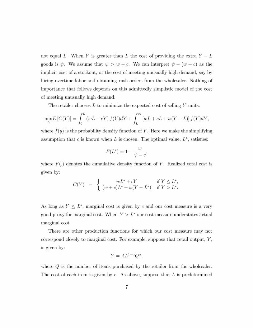
not equal L. When Y is greater than L the cost of providing the extra Y � L

goods is . We assume that > w + c. We can interpret � (w + c) as the

implicit cost of a stockout, or the cost of meeting unusually high demand, say by

hiring overtime labor and obtaining rush orders from the wholesaler. Nothing of

importance that follows depends on this admittedly simplistic model of the cost

of meeting unusually high demand.

The retailer chooses L to minimize the expected cost of selling Y units:

minLE [C(Y )] =

Z L

0

(wL+ cY ) f(Y )dY +

Z 1

L

[wL+ cL+ (Y � L)] f(Y )dY ,

where f(y) is the probability density function of Y . Here we make the simplifying

assumption that c is known when L is chosen. The optimal value, L�, satis�es:

F (L�) = 1� w

� c,

where F (:) denotes the cumulative density function of Y . Realized total cost is

given by:

C(Y ) =

�wL� + cY

(w + c)L� + (Y � L�)if Y � L�,if Y > L�.

As long as Y � L�, marginal cost is given by c and our cost measure is a very

good proxy for marginal cost. When Y > L� our cost measure understates actual

marginal cost.

There are other production functions for which our cost measure may not

correspond closely to marginal cost. For example, suppose that retail output, Y ,

is given by:

Y = AL1��Q�,

where Q is the number of items purchased by the retailer from the wholesaler.

The cost of each item is given by c. As above, suppose that L is predetermined

7

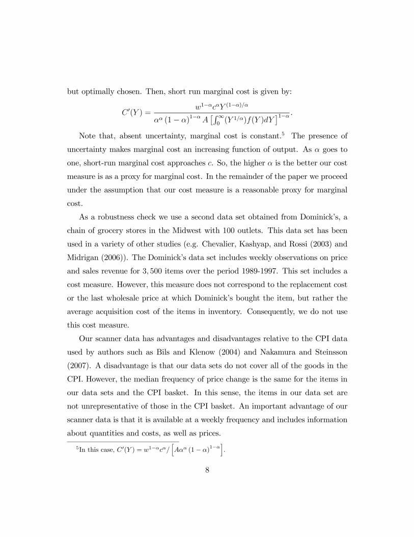
but optimally chosen. Then, short run marginal cost is given by:

C 0(Y ) =w1��c�Y (1��)=�

�� (1� �)1��A�R10(Y 1=�)f(Y )dY

�1�� .Note that, absent uncertainty, marginal cost is constant.5 The presence of

uncertainty makes marginal cost an increasing function of output. As � goes to

one, short-run marginal cost approaches c. So, the higher � is the better our cost

measure is as a proxy for marginal cost. In the remainder of the paper we proceed

under the assumption that our cost measure is a reasonable proxy for marginal

cost.

As a robustness check we use a second data set obtained from Dominick�s, a

chain of grocery stores in the Midwest with 100 outlets. This data set has been

used in a variety of other studies (e.g. Chevalier, Kashyap, and Rossi (2003) and

Midrigan (2006)). The Dominick�s data set includes weekly observations on price

and sales revenue for 3; 500 items over the period 1989-1997. This set includes a

cost measure. However, this measure does not correspond to the replacement cost

or the last wholesale price at which Dominick�s bought the item, but rather the

average acquisition cost of the items in inventory. Consequently, we do not use

this cost measure.

Our scanner data has advantages and disadvantages relative to the CPI data

used by authors such as Bils and Klenow (2004) and Nakamura and Steinsson

(2007). A disadvantage is that our data sets do not cover all of the goods in the

CPI. However, the median frequency of price change is the same for the items in

our data sets and the CPI basket. In this sense, the items in our data set are

not unrepresentative of those in the CPI basket. An important advantage of our

scanner data is that it is available at a weekly frequency and includes information

about quantities and costs, as well as prices.

5In this case, C 0(Y ) = w1��c�=hA�� (1� �)1��

i.

8

Given the large number of items in our data set we must adopt a procedure

to parsimoniously report our �ndings. Unless stated otherwise, the statistics that

we report are computed as follows. First, we calculate the median value of a

statistic across all items in a given category. We then compute the median of the

200 category medians. As a robustness check we also report results for revenue-

weighted medians across categories.

3. The behavior of weekly prices and reference prices

In this section we compare the behavior of weekly and reference prices. Recall that

the reference price of an item is the most commonly observed price for that item

within a quarter. We refer to all other prices as nonreference prices. Our basic

�ndings in this section are twofold. First, according to various metrics reference

prices are important. Second, reference prices are much more persistent than

weekly prices.

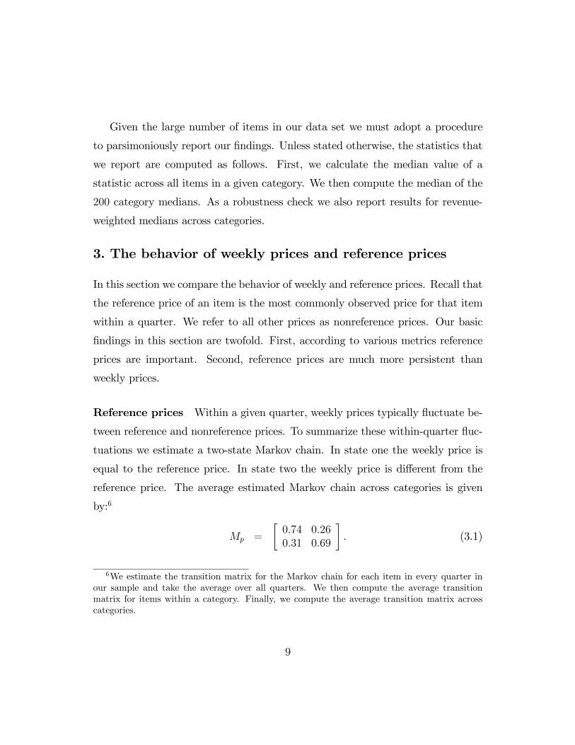
Reference prices Within a given quarter, weekly prices typically �uctuate be-

tween reference and nonreference prices. To summarize these within-quarter �uc-

tuations we estimate a two-state Markov chain. In state one the weekly price is

equal to the reference price. In state two the weekly price is di¤erent from the

reference price. The average estimated Markov chain across categories is given

by:6

Mp =

�0:740:31

0:260:69

�. (3.1)

6We estimate the transition matrix for the Markov chain for each item in every quarter inour sample and take the average over all quarters. We then compute the average transitionmatrix for items within a category. Finally, we compute the average transition matrix acrosscategories.

9

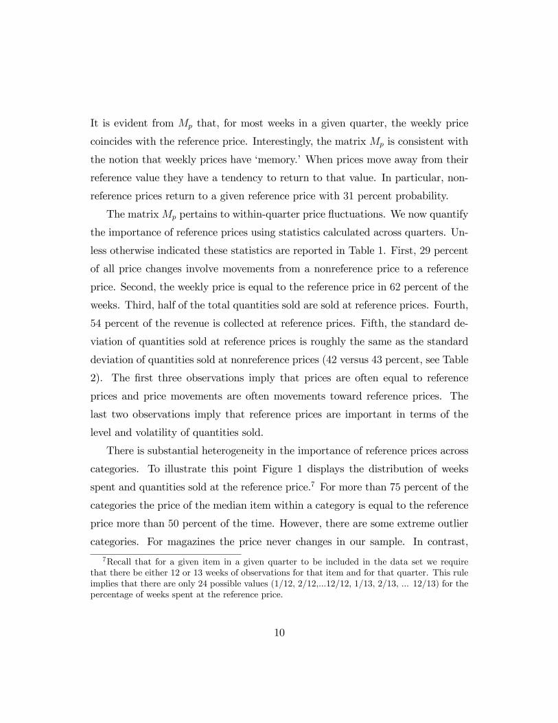
It is evident from Mp that, for most weeks in a given quarter, the weekly price

coincides with the reference price. Interestingly, the matrix Mp is consistent with

the notion that weekly prices have �memory.�When prices move away from their

reference value they have a tendency to return to that value. In particular, non-

reference prices return to a given reference price with 31 percent probability.

The matrixMp pertains to within-quarter price �uctuations. We now quantify

the importance of reference prices using statistics calculated across quarters. Un-

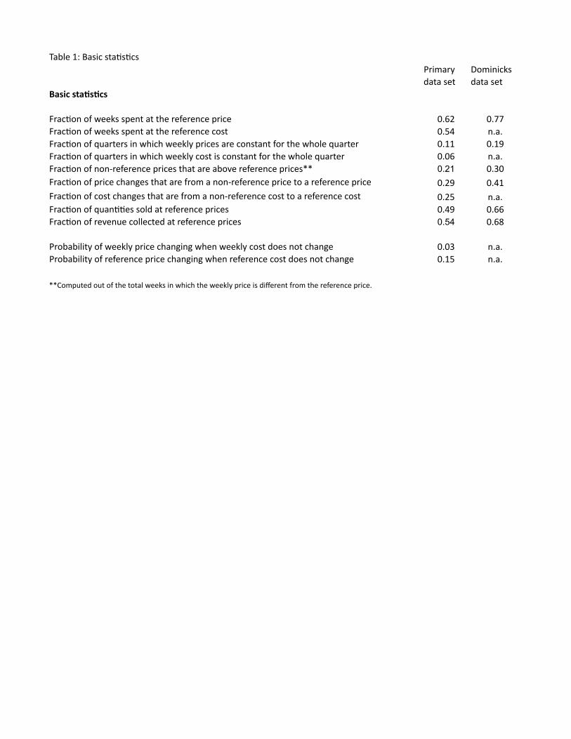
less otherwise indicated these statistics are reported in Table 1. First, 29 percent

of all price changes involve movements from a nonreference price to a reference

price. Second, the weekly price is equal to the reference price in 62 percent of the

weeks. Third, half of the total quantities sold are sold at reference prices. Fourth,

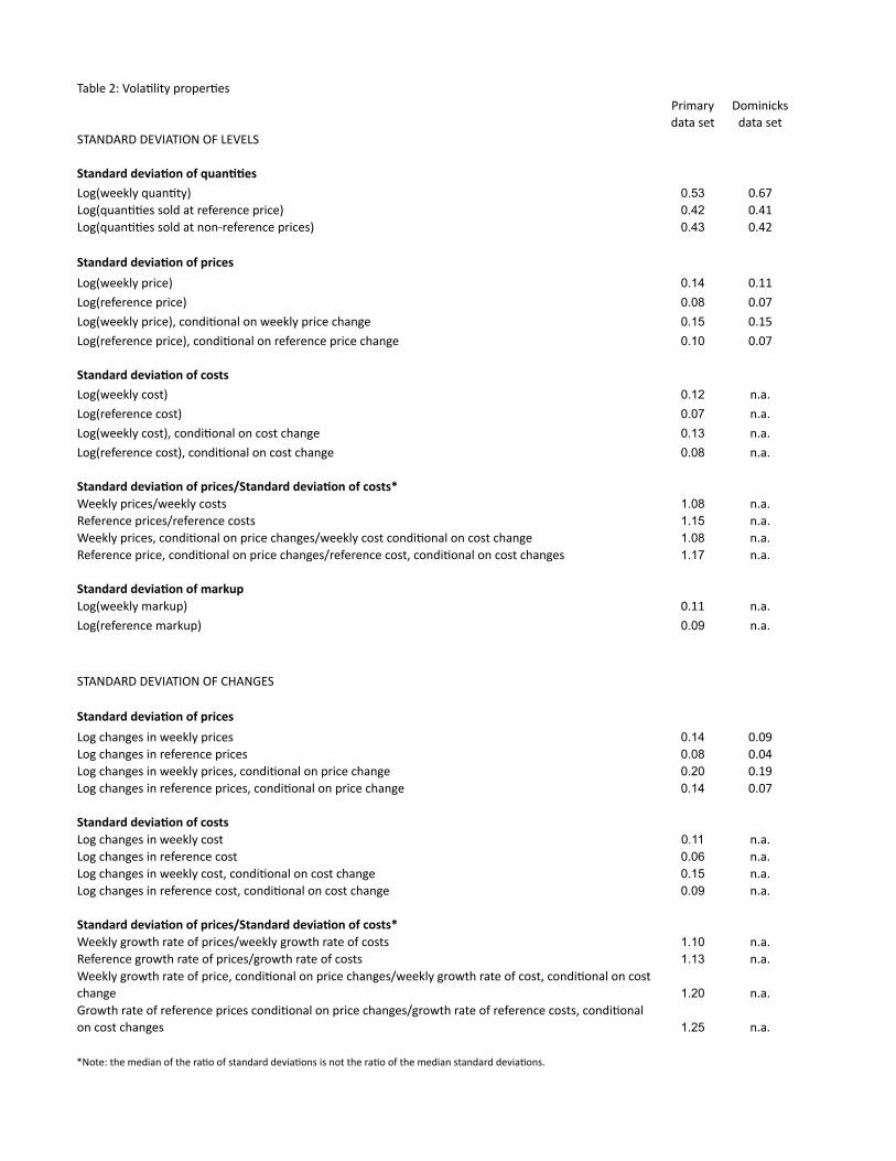
54 percent of the revenue is collected at reference prices. Fifth, the standard de-

viation of quantities sold at reference prices is roughly the same as the standard

deviation of quantities sold at nonreference prices (42 versus 43 percent, see Table

2). The �rst three observations imply that prices are often equal to reference

prices and price movements are often movements toward reference prices. The

last two observations imply that reference prices are important in terms of the

level and volatility of quantities sold.

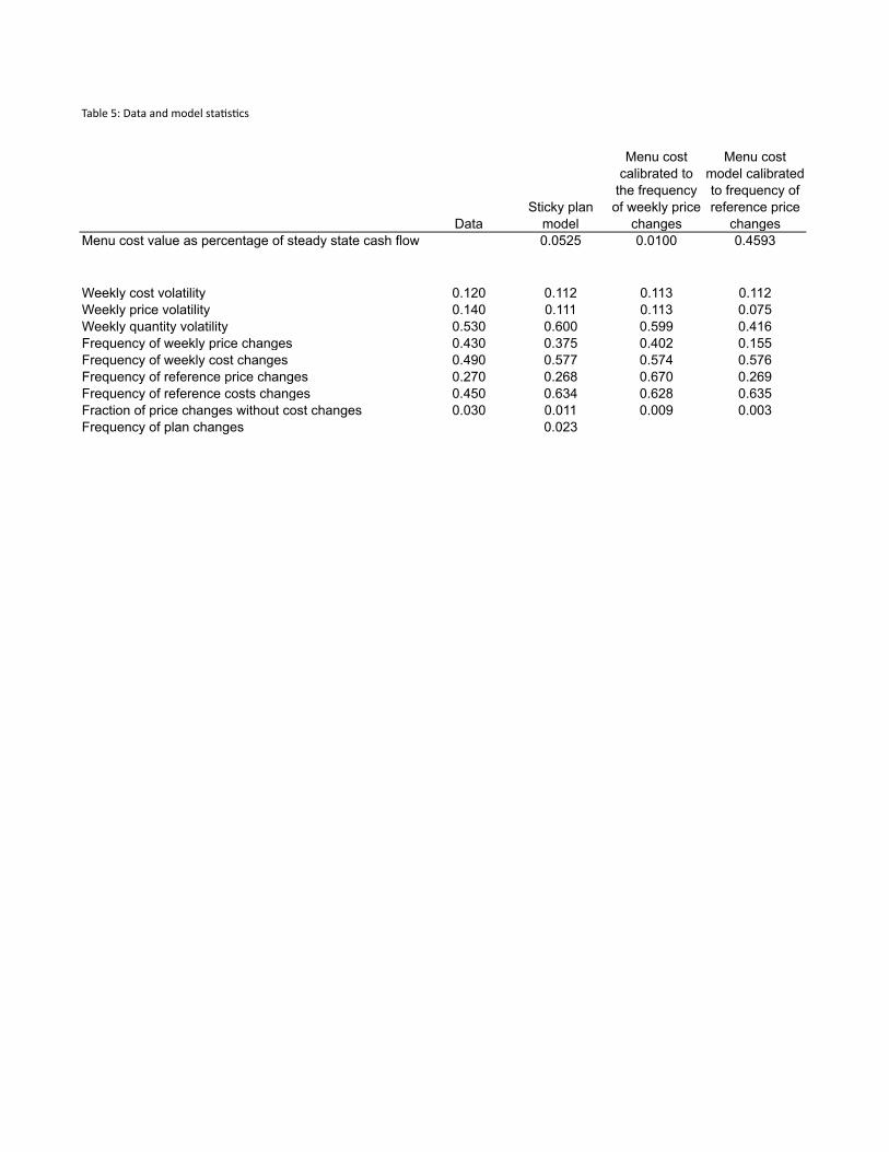
There is substantial heterogeneity in the importance of reference prices across

categories. To illustrate this point Figure 1 displays the distribution of weeks

spent and quantities sold at the reference price.7 For more than 75 percent of the

categories the price of the median item within a category is equal to the reference

price more than 50 percent of the time. However, there are some extreme outlier

categories. For magazines the price never changes in our sample. In contrast,

7Recall that for a given item in a given quarter to be included in the data set we requirethat there be either 12 or 13 weeks of observations for that item and for that quarter. This ruleimplies that there are only 24 possible values (1/12, 2/12,...12/12, 1/13, 2/13, ... 12/13) for thepercentage of weeks spent at the reference price.

10

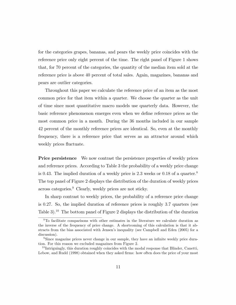
for the categories grapes, bananas, and pears the weekly price coincides with the

reference price only eight percent of the time. The right panel of Figure 1 shows

that, for 70 percent of the categories, the quantity of the median item sold at the

reference price is above 40 percent of total sales. Again, magazines, bananas and

pears are outlier categories.

Throughout this paper we calculate the reference price of an item as the most

common price for that item within a quarter. We choose the quarter as the unit

of time since most quantitative macro models use quarterly data. However, the

basic reference phenomenon emerges even when we de�ne reference prices as the

most common price in a month. During the 36 months included in our sample

42 percent of the monthly reference prices are identical. So, even at the monthly

frequency, there is a reference price that serves as an attractor around which

weekly prices �uctuate.

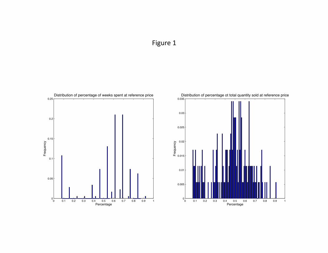
Price persistence We now contrast the persistence properties of weekly prices

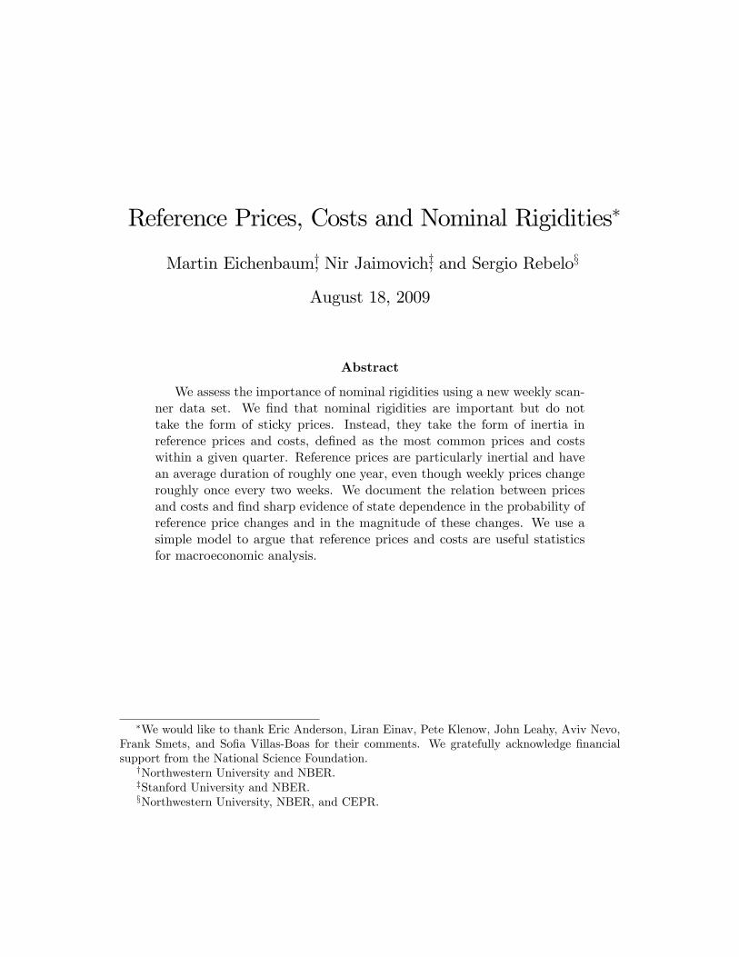
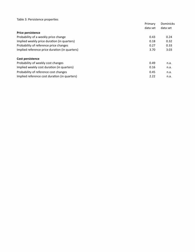
and reference prices. According to Table 3 the probability of a weekly price change

is 0:43. The implied duration of a weekly price is 2:3 weeks or 0:18 of a quarter.8

The top panel of Figure 2 displays the distribution of the duration of weekly prices

across categories.9 Clearly, weekly prices are not sticky.

In sharp contrast to weekly prices, the probability of a reference price change

is 0:27. So, the implied duration of reference prices is roughly 3:7 quarters (see

Table 3).10 The bottom panel of Figure 2 displays the distribution of the duration

8To facilitate comparisons with other estimates in the literature we calculate duration asthe inverse of the frequency of price change. A shortcoming of this calculation is that it ab-stracts from the bias associated with Jensen�s inequality (see Campbell and Eden (2005) for adiscussion).

9Since magazine prices never change in our sample, they have an in�nite weekly price dura-tion. For this reason we excluded magazines from Figure 2.10Intriguingly, this duration roughly coincides with the modal response that Blinder, Canetti,

Lebow, and Rudd (1998) obtained when they asked �rms: how often does the price of your most

11

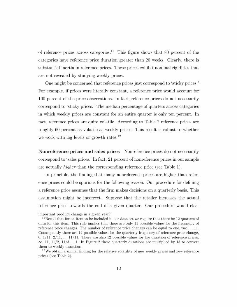
of reference prices across categories.11 This �gure shows that 80 percent of the

categories have reference price duration greater than 20 weeks. Clearly, there is

substantial inertia in reference prices. These prices exhibit nominal rigidities that

are not revealed by studying weekly prices.

One might be concerned that reference prices just correspond to �sticky prices.�

For example, if prices were literally constant, a reference price would account for

100 percent of the price observations. In fact, reference prices do not necessarily

correspond to �sticky prices.�The median percentage of quarters across categories

in which weekly prices are constant for an entire quarter is only ten percent. In

fact, reference prices are quite volatile. According to Table 2 reference prices are

roughly 60 percent as volatile as weekly prices. This result is robust to whether

we work with log levels or growth rates.12

Nonreference prices and sales prices Nonreference prices do not necessarily

correspond to �sales prices.�In fact, 21 percent of nonreference prices in our sample

are actually higher than the corresponding reference price (see Table 1).

In principle, the �nding that many nonreference prices are higher than refer-

ence prices could be spurious for the following reason. Our procedure for de�ning

a reference price assumes that the �rm makes decisions on a quarterly basis. This

assumption might be incorrect. Suppose that the retailer increases the actual

reference price towards the end of a given quarter. Our procedure would clas-

important product change in a given year?11Recall that for an item to be included in our data set we require that there be 12 quarters of

data for this item. This rule implies that there are only 11 possible values for the frequency ofreference price changes. The number of reference price changes can be equal to one, two,..., 11.Consequently there are 12 possible values for the quarterly frequency of reference price change,0, 1/11, 2/11, ... 11/11. There are also 12 possible values for the duration of reference prices:1, 11, 11/2, 11/3,... 1. In Figure 2 these quarterly durations are multiplied by 13 to convertthem to weekly durations.12We obtain a similar �nding for the relative volatility of new weekly prices and new reference

prices (see Table 2).

12

sify those prices as nonreference prices that are higher than the reference price.

Similarly, suppose the retailer lowers the reference price near the beginning of the

quarter. Our procedure would classify the actual old reference prices that occur

in the beginning of the quarter as higher than the measured reference price for

that quarter.

To produce an upper bound on the quantitative importance of these two sce-

narios we compute the fraction of the high nonreference prices that are not equal

to the reference price in the previous or subsequent quarter. We �nd that this

fraction is equal to 60 percent. So, a lower bound for the fraction of nonreference

prices that are actually higher than the corresponding reference price is 12 percent

(0:21 times 0:60). Taken as a whole our results indicate that nonreference prices

are not necessarily �sale prices.�

Some robustness checks As discussed above there can be spurious changes

in prices in our data set associated with the time-varying use of loyalty cards,

coupons, and promotions. Consequently, our estimate of the duration of weekly

prices (0:18 of a quarter) is a lower bound on the true duration of weekly prices.

From this perspective prices could be more inertial than suggested by our point

estimates. We use two approaches to assess the potential impact of measurement

error on our duration estimates.

First, we recompute the probability of a price change assuming that an actual

price change occurs only when our price measure changes by more than x percent,

for x = 1, 2, : : :,5. Weekly price duration is an increasing function of x and peaks

at 0:27 of a quarter when x = 5 (recall that our benchmark value of weekly price

duration is 0:18 of a quarter). Signi�cantly, the reference price duration remains

equal to our benchmark estimate of 3:7 quarters for all the values of x that we

consider. So, the basic �nding that reference prices are much more persistent than

13

weekly prices is una¤ected by this type of measurement error.

Second, we use an additional data set from the retailer that contains the actual

price associated with each transaction for 374 stores in Arizona, California, Col-

orado, Oregon, Washington, and Wyoming. Because prices are observed directly,

there is no measurement error associated with the time-varying use of discounts,

coupons, loyalty cards, and other promotions. This data set is only available for

a short time period (January 4 to December 31, 2004). The average number of

days in which we observe the same item is 14. So, while we cannot use this data

set to compute price duration, we can use it to quantify the bias introduced by

the use of unit-value prices.

For the new data set we identify all UPCs that are sold three or more times

in the same store in the same day and are included in the data for at least seven

days. There are 1:7 million such observations. In 70 percent of these observations

the same good is sold at the same price in all transactions that occur in the same

store and on the same day. So, in this data set, measurement error can at most

a¤ect 30 percent of the observations. We can use this statistic to quantify the

impact of measurement error on the duration of weekly prices. The probability of

a weekly price change is 0:41. Suppose that 30 percent of these changes are indeed

spurious. Then, the true probability of a weekly price change is 0:7� 0:41 = 0:29.This probability of a weekly price change implies a duration of weekly prices of

0:27 quarters. Interestingly, this estimate coincides with the one we obtained

using our �rst method for assessing the importance of measurement error.

This new data set is not long enough to allow us to compute reference prices.

But any correction for measurement error would only increase the duration of

reference prices. So, by correcting the duration of weekly prices but not the dura-

tion of reference prices we are providing a conservative estimate of the di¤erence

between the two. This estimate is 3:43 quarters (3:7 � 0:27). We conclude that,

14

even taking measurement error into account, the duration of reference prices is

much longer than the duration of weekly prices.

Our main results pertain to statistics calculated using medians across cate-

gories. To assess the robustness of these results we also compute statistics using

revenue-weighted medians across categories. We �nd that, with one possible ex-

ception, our results are robust to this alternative procedure. The one exception

is that the point estimate of the duration of reference prices goes from 3:7 to 2:7

quarters. The duration of weekly prices is essentially unchanged. So, the ba-

sic qualitative result that reference prices are much more persistent than weekly

prices is una¤ected.

Results for Dominick�s data set We conclude this section by brie�y dis-

cussing the results that we obtain with the Dominick�s data set. As Tables 1

through 3 show, these results are very similar to those obtained with our primary

data set. Reference prices are important. First, weekly prices are often equal to

reference prices (77 percent of the weeks). Second, price movements are often

movements toward reference prices. The fraction of price changes that are from a

nonreference price to a reference price is 41 percent. Third, reference prices con-

tinue to be important in terms of the fraction of quantities sold at reference prices

(66 percent) and the volatility of quantities sold at reference prices (41 percent).

Finally, we �nd the same sharp contrast between the duration of weekly and

reference prices. The duration of weekly prices is 0:32 quarters while the duration

of reference prices is roughly three quarters.

4. The behavior of weekly costs and reference costs

In this section we compare the behavior of weekly and reference costs. The latter

is de�ned as the most commonly observed cost for that item within a quarter. We

15

refer to all other costs as nonreference costs. Our basic �ndings in this section can

be summarized as follows. First, judging by various measures, reference cost are

important. Second, reference costs are much more persistent than weekly costs.

Third, reference costs are less persistent than reference prices.

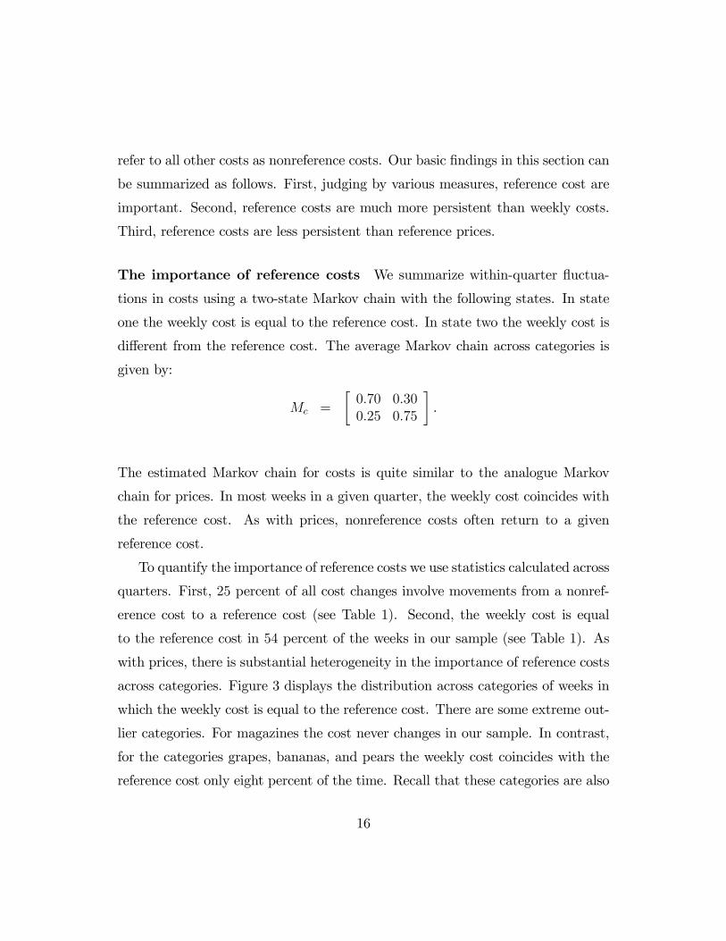
The importance of reference costs We summarize within-quarter �uctua-

tions in costs using a two-state Markov chain with the following states. In state

one the weekly cost is equal to the reference cost. In state two the weekly cost is

di¤erent from the reference cost. The average Markov chain across categories is

given by:

Mc =

�0:700:25

0:300:75

�.

The estimated Markov chain for costs is quite similar to the analogue Markov

chain for prices. In most weeks in a given quarter, the weekly cost coincides with

the reference cost. As with prices, nonreference costs often return to a given

reference cost.

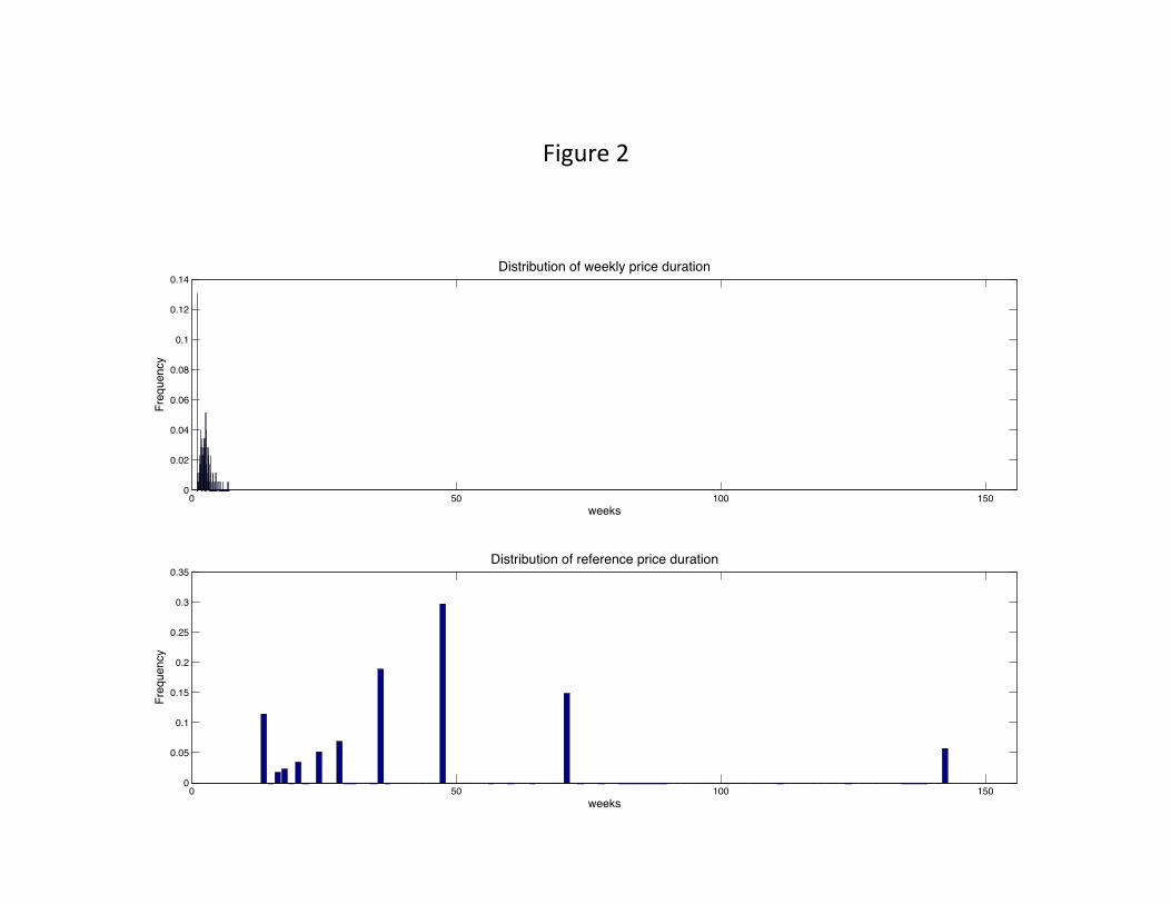
To quantify the importance of reference costs we use statistics calculated across

quarters. First, 25 percent of all cost changes involve movements from a nonref-

erence cost to a reference cost (see Table 1). Second, the weekly cost is equal

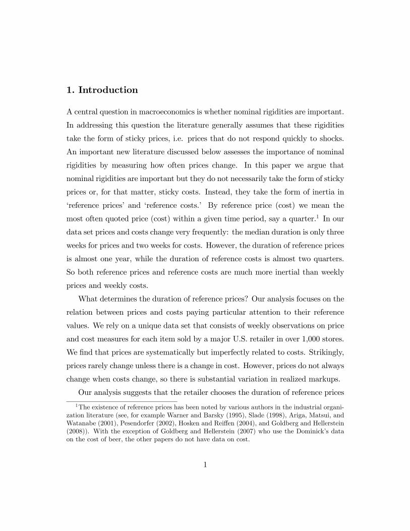
to the reference cost in 54 percent of the weeks in our sample (see Table 1). As

with prices, there is substantial heterogeneity in the importance of reference costs

across categories. Figure 3 displays the distribution across categories of weeks in

which the weekly cost is equal to the reference cost. There are some extreme out-

lier categories. For magazines the cost never changes in our sample. In contrast,

for the categories grapes, bananas, and pears the weekly cost coincides with the

reference cost only eight percent of the time. Recall that these categories are also

16

outliers in terms of the fraction of weeks in which the weekly price is equal to the

reference price.

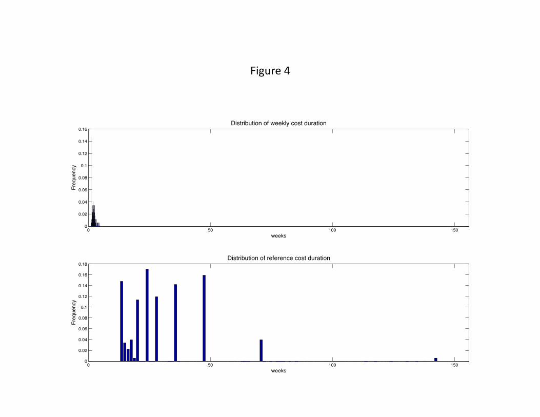
Cost persistence As with prices, there is a sharp contrast between the persis-

tence properties of weekly costs and reference costs. From Table 3 we see that

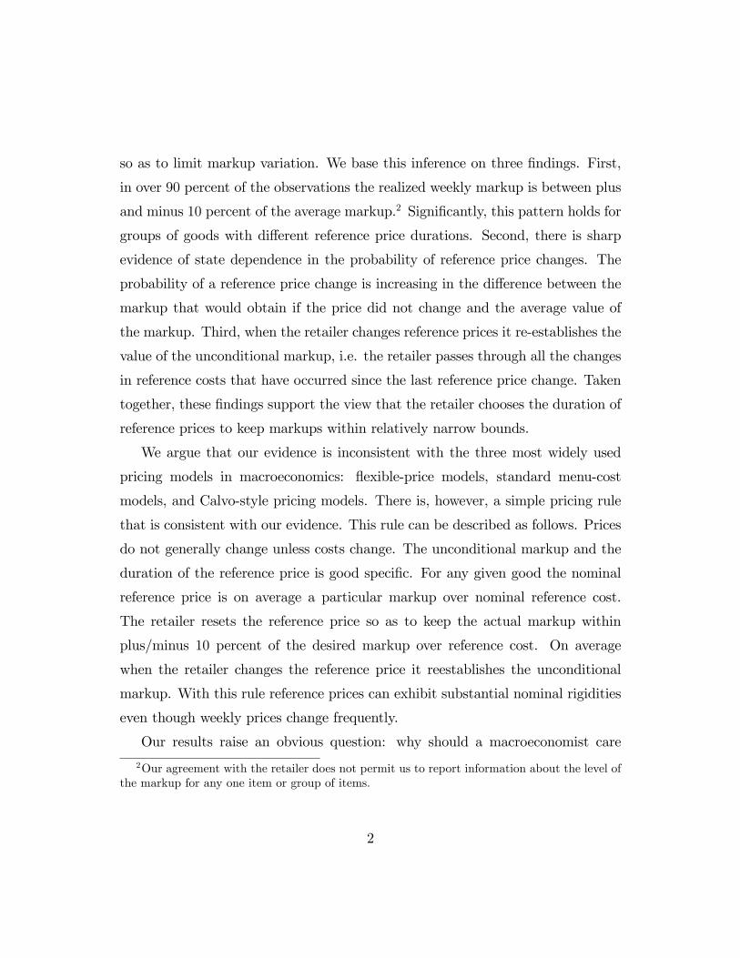
the probability of a weekly cost change is 0:49. So, the implied duration of a

weekly cost is 0:16 of a quarter, or roughly 2:1 weeks. The top panel of Figure

4 displays the distribution of duration of weekly costs across categories. Clearly,

weekly costs are not sticky.

The probability of a reference cost change is 0:45. So, the implied duration

of reference costs is roughly 2:2 quarters. The bottom panel of Figure 4 displays

the distribution of reference cost duration across categories. Roughly two-thirds

of the categories have reference cost duration exceeding 20 weeks. Clearly, there

is substantial inertia in reference costs. The existence of stickiness in costs would

not be revealed by analyzing weekly costs.

As with reference prices, one might be concerned that reference costs just

correspond to sticky costs. This concern is not warranted. Across all categories,

the median percentage of quarters in which weekly costs are constant is only six

percent. In fact reference costs are quite volatile. According to Table 2 reference

costs are roughly 60 percent as volatile as weekly costs.13

We conclude this section by noting that our weekly cost measures can have an

endogenous component associated with trade promotions. As discussed in Mara-

tou (2006) and Maratou, Gómez, and Just (2004), there are basically two types

of trade promotions: performance-based contracts and discount-based contracts.

Performance-based contracts give retailers incentives to sell the manufacturer�s

product. These incentives are tied to a measure of retailer performance (e.g.,

13We obtain a similar �nding for the relative volatility of new weekly costs and new referencecosts (see Table 2).

17

units sold, displayed or price discounts in e¤ect during a given period). We think

of these contracts as exogenous price schedules that are non-linear in nature. The

main impact of this non-linearity is to potentially introduce measurement error

into our analysis by driving a wedge between the retailer�s average and marginal

cost.

Discount-based promotions can induce a di¤erent type of endogeneity. These

promotions generally take the following form: suppliers provide merchandise to

retailers at a discount, usually for a brief, speci�ed period (two to three weeks

is standard). Changes in cost and prices induced by these types of promotions

are likely to be transitory in nature. For this reason they are unlikely to a¤ect

reference costs and prices, which have an average duration of six months and one

year, respectively.

5. The determinants of price changes

In this section we investigate the relation between reference prices and costs and

�nd that there is a very important form of state dependence in reference prices.

Speci�cally, the duration of reference prices is chosen to limit markup varation.

This �nding is based on four observations that we document below. First, the

duration of reference prices is such that the variation of markups within the spell of

a reference price is within �10% of the average markup. Second, there is evidenceof state dependence in the probability of reference price changes. Third, when

the retailer changes reference prices it reestablishes the value of the unconditional

markup. Finally, in periods in which the reference price is constant before it rises

(falls), the markup falls (rises).

The relation between prices and cost changes A striking property of our

data is that prices generally do not change absent a change in costs. The probabil-

18

ity that the weekly price changes without a change in the weekly cost is only three

percent (see Table 1). The probability that the reference price changes without a

change in reference cost is 15 percent.

We do not �nd an important lag or lead in the relation between changes in

costs and changes in prices. We assess whether there is a lag in the response of

prices to changes in cost by computing the probability of a price change at time

t+ 1, conditional on a cost change occurring at time t, no price change occurring

at time t, and no cost change occurring at t+ 1. This probability is four percent

and 15 percent for weekly and reference prices, respectively. So, there does not

seem to be an important lag in the response of prices to changes in costs.

To see if there is a lead in the response of prices to changes in cost we compute

the probability of a price change at time t � 1, conditional on a cost changeoccurring at time t, no price change occurring at time t, and no cost change

occurring at t� 1. This probability is four percent and 16 percent for weekly andreference prices, respectively. These results suggest that there are no important

leads in the response of prices to changes in costs.

While prices generally do not change absent a change in costs, a change in

cost is not su¢ cient to induce a change in price. This fact means that there are

substantial variations in markups. According to Table 2 the standard deviation of

the weekly markup is 11 percent. The standard deviation of the reference markup,

de�ned as the standard deviation of the ratio of reference prices to reference costs,

is 9 percent.

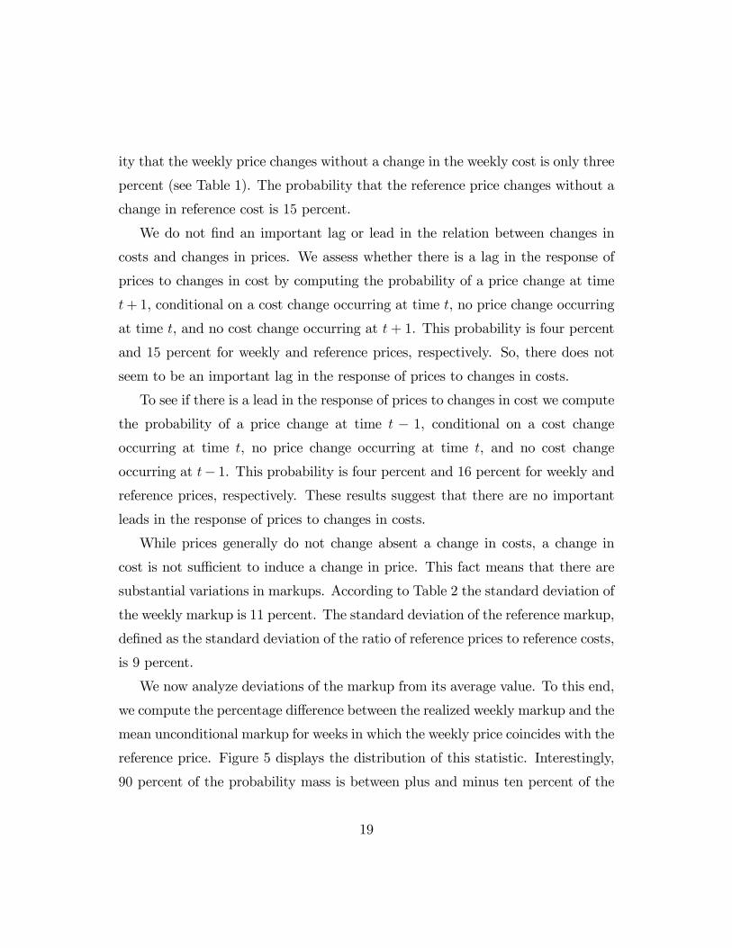
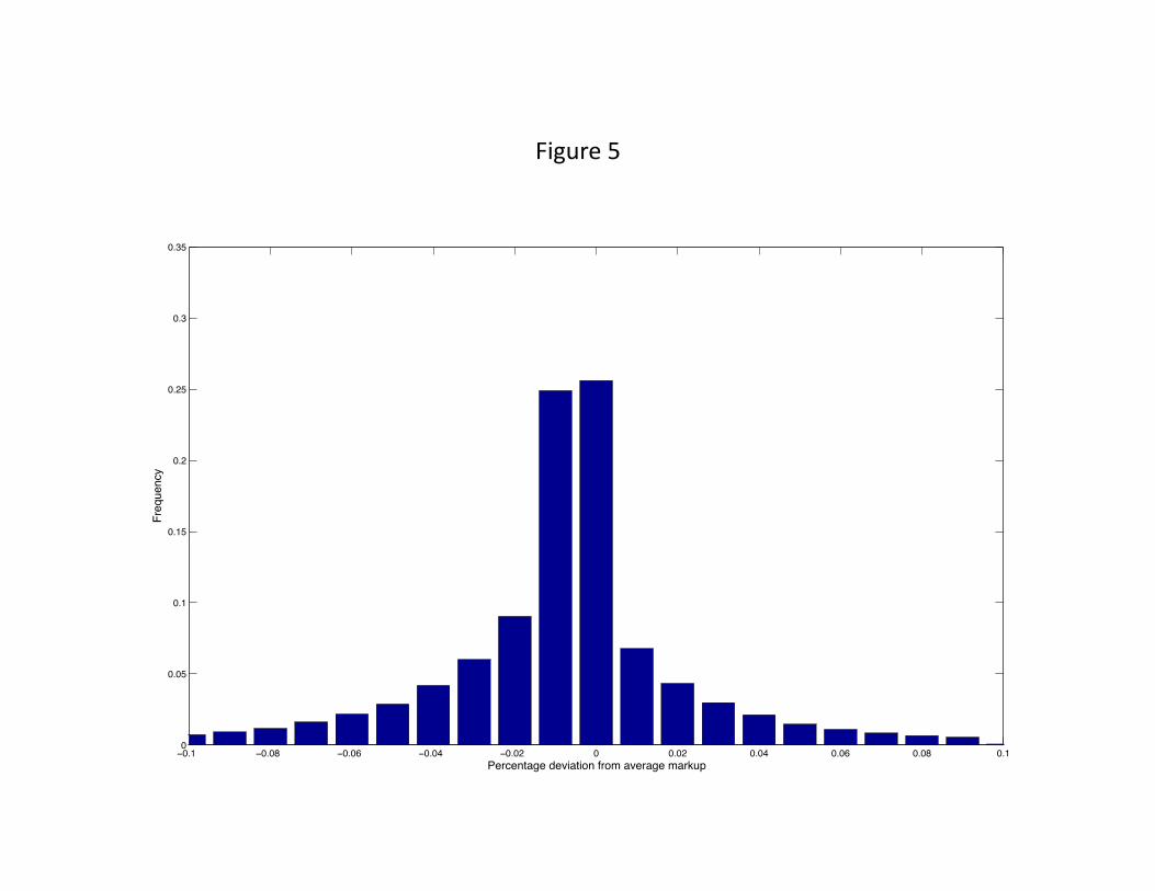
We now analyze deviations of the markup from its average value. To this end,

we compute the percentage di¤erence between the realized weekly markup and the

mean unconditional markup for weeks in which the weekly price coincides with the

reference price. Figure 5 displays the distribution of this statistic. Interestingly,

90 percent of the probability mass is between plus and minus ten percent of the

19

average markup. This �nding suggests that the retailer resets its reference prices

so that variations in the realized markup fall within a reasonably small interval.

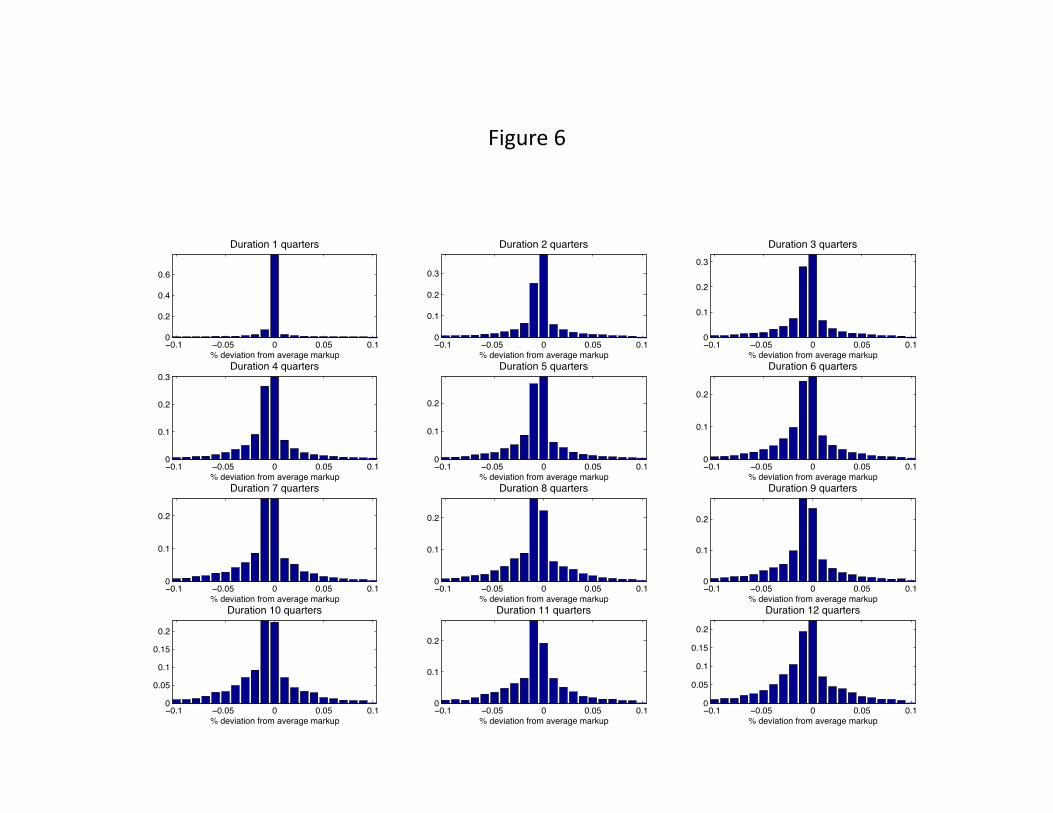
To assess this hypothesis, we compute the analogue of Figure 5 for di¤erent

categories of goods, classi�ed according to the median duration of the reference

price. The results are displayed in Figure 6 for groups of goods with median

durations ranging from one to twelve quarters. These distributions are generally

similar to those displayed in Figure 5. This �nding is consistent with the hy-

pothesis that the retailer chooses the duration of the reference price for each item

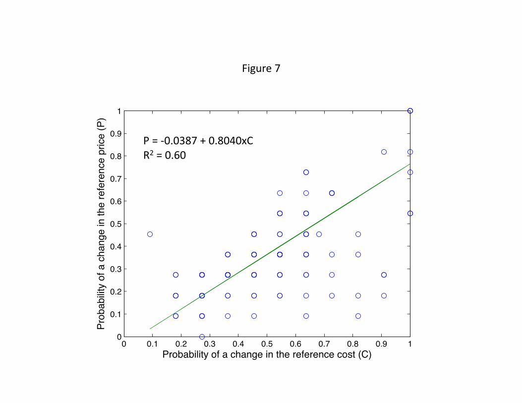
to keep realized markups within similar small bounds. Figure 7 provides further

evidence in support of this hypothesis. This �gure shows that categories with a

high probability of a reference cost change have a high probability of a reference

price change.14

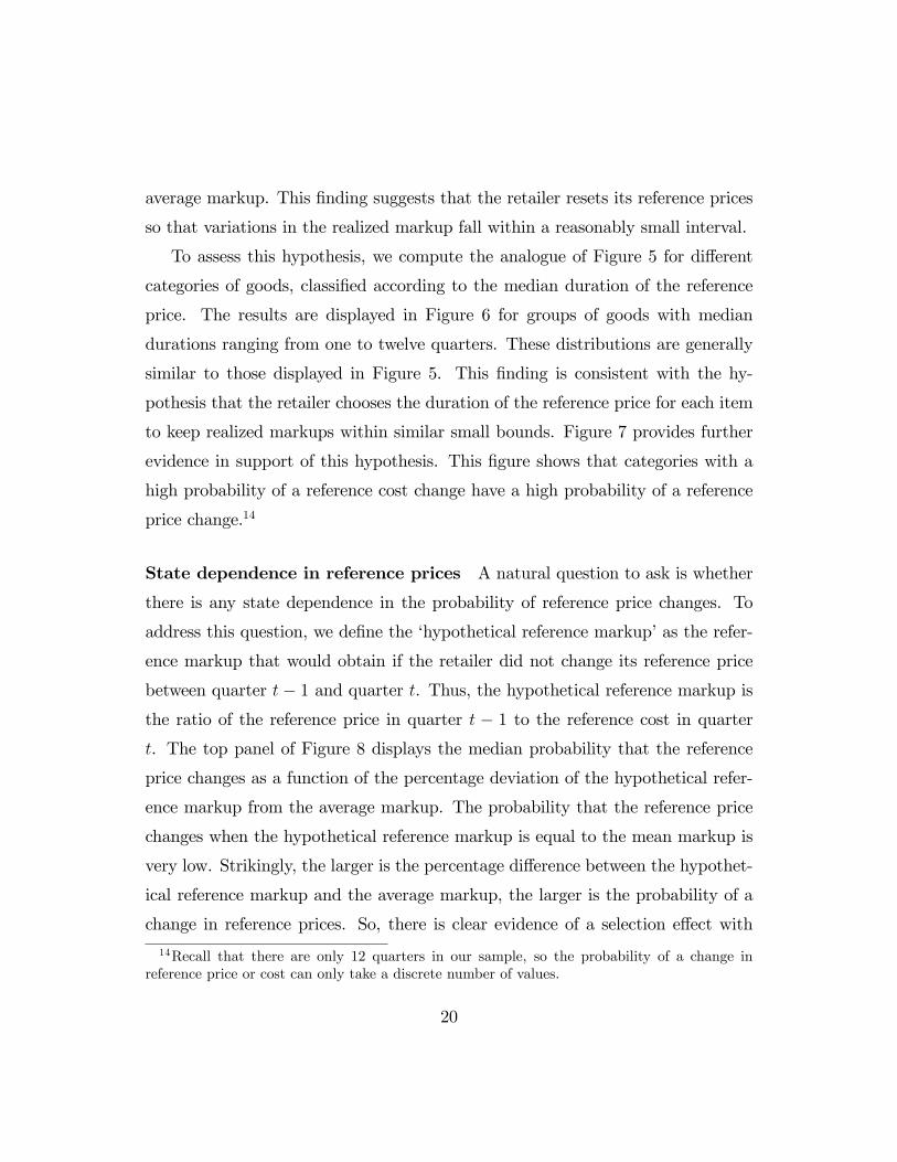
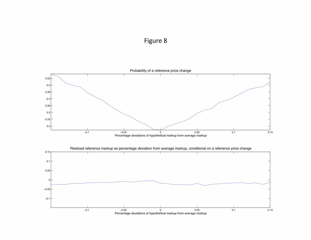
State dependence in reference prices A natural question to ask is whether

there is any state dependence in the probability of reference price changes. To

address this question, we de�ne the �hypothetical reference markup�as the refer-

ence markup that would obtain if the retailer did not change its reference price

between quarter t� 1 and quarter t. Thus, the hypothetical reference markup isthe ratio of the reference price in quarter t � 1 to the reference cost in quartert. The top panel of Figure 8 displays the median probability that the reference

price changes as a function of the percentage deviation of the hypothetical refer-

ence markup from the average markup. The probability that the reference price

changes when the hypothetical reference markup is equal to the mean markup is

very low. Strikingly, the larger is the percentage di¤erence between the hypothet-

ical reference markup and the average markup, the larger is the probability of a

change in reference prices. So, there is clear evidence of a selection e¤ect with

14Recall that there are only 12 quarters in our sample, so the probability of a change inreference price or cost can only take a discrete number of values.

20

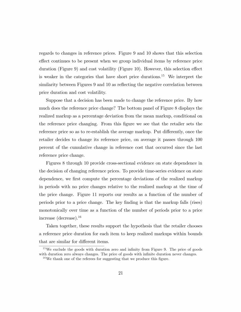
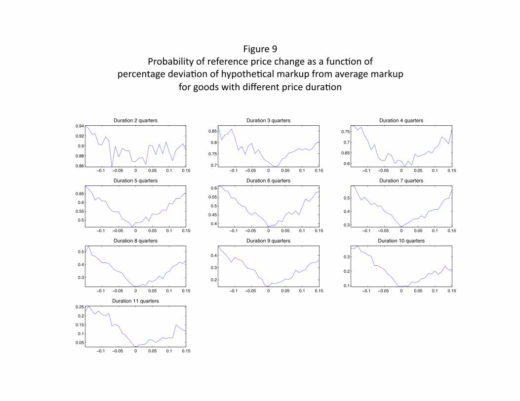
regards to changes in reference prices. Figure 9 and 10 shows that this selection

e¤ect continues to be present when we group individual items by reference price

duration (Figure 9) and cost volatility (Figure 10). However, this selection e¤ect

is weaker in the categories that have short price durations.15 We interpret the

similarity between Figures 9 and 10 as re�ecting the negative correlation between

price duration and cost volatility.

Suppose that a decision has been made to change the reference price. By how

much does the reference price change? The bottom panel of Figure 8 displays the

realized markup as a percentage deviation from the mean markup, conditional on

the reference price changing. From this �gure we see that the retailer sets the

reference price so as to re-establish the average markup. Put di¤erently, once the

retailer decides to change its reference price, on average it passes through 100

percent of the cumulative change in reference cost that occurred since the last

reference price change.

Figures 8 through 10 provide cross-sectional evidence on state dependence in

the decision of changing reference prices. To provide time-series evidence on state

dependence, we �rst compute the percentage deviations of the realized markup

in periods with no price changes relative to the realized markup at the time of

the price change. Figure 11 reports our results as a function of the number of

periods prior to a price change. The key �nding is that the markup falls (rises)

monotonically over time as a function of the number of periods prior to a price

increase (decrease).16

Taken together, these results support the hypothesis that the retailer chooses

a reference price duration for each item to keep realized markups within bounds

that are similar for di¤erent items.15We exclude the goods with duration zero and in�nity from Figure 9. The price of goods

with duration zero always changes. The price of goods with in�nite duration never changes.16We thank one of the referees for suggesting that we produce this �gure.

21

6. Other features of the data

In this section we document two additional features of the data that are useful for

evaluating the plausibility of di¤erent pricing models.

Volatility of prices and marginal cost In our data set prices are more volatile

than our measure of marginal cost. This result holds for weekly prices and costs

as well as for reference prices and costs. The basic intuition for this result is that

prices often do not change much in response to small changes in cost. But small

cost changes that cumulate and create large deviations from the average markup

can trigger very large changes in price. This pattern of behavior generates prices

that have a larger standard deviation than cost.

The median of the ratio of the standard deviation of log(weekly price) to the

standard deviation of log(weekly cost) is 1:08. The median of the ratio of the stan-

dard deviation of log(reference price) to the standard deviation of log(reference

cost) is 1:15. We also �nd that prices are more volatile than costs if we focus on

new prices and new costs or if we work in growth rates (see Table 2). We conclude

that, regardless of whether we work with weekly or reference prices and costs, the

volatility of prices generally exceeds that of marginal cost.

Demand shocks Conditional on the weekly price being constant and equal

to the reference price, the standard deviation of quantities sold is roughly 42

percent.17 This conditional volatility is roughly 79 percent of the unconditional

volatility of quantities sold. We infer that demand shocks are quantitatively im-

portant.

17A caveat to our calculation is that we are conditioning on the nominal price being constantinstead of the real price being constant. By real price we mean the price of the good relativeto the CPI basket. Since we focus on a short time period during which in�ation is quite low, itseems unlikely that in�ation e¤ects are important for this calculation.

22

7. Reconciling di¤erent pricing models with our �ndings

In this section we discuss the implications of our empirical �ndings for three pricing

models that are widely used in macroeconomics: �exible price models, menu cost

models, and Calvo models.

Flexible price models The Dixit-Stiglitz model of monopolistic competition

lies at the core of many �exible price macroeconomic models. In this model, the

elasticity of substitution across di¤erent goods is constant. The optimal policy

for each monopolist is to set the price (Pt) equal to a constant markup (�) over

marginal cost (Ct), Pt = �Ct. This model is clearly inconsistent with our data,

since it implies that there should be no variation in the markup. Table 2 indicates

that the standard deviation of the logarithm of the realized weekly markup and

reference markup is 0:11 and 0:09, respectively.

It is possible to reconcile a �exible price model with the data by introduc-

ing demand shocks that generate markup �uctuations. But, matching the data

requires an incredible con�guration of cost and demand shocks. Consider the

following simple speci�cation in which demand is linear:

Pt = at � btQt,

where Qt represents the quantity sold. The variables at and bt are stochastic

demand shifters. Variable pro�ts, �t are given by: �t = PtQt �CtQt, where Ct is

the monopolist�s cost. The monopolist�s optimal price and quantity are given by:

P �t =at + Ct2

,

Q�t =at � Ct2bt

.

23

Changes in bt only a¤ect the quantity sold. Changes in at a¤ect both price

and quantity. Given observations on P �t , Q�t , and Ct, we can deduce the time

series for at and bt such that P �t and Q�t match the data exactly. We perform

this calculation for each of the items in our sample. Three key results emerge.

First, the median standard deviation of log(at) and log(bt) are 0:16 and 0:77,

respectively. So, to match the data the variable at must be roughly as as volatile

as prices and cost (see Table 2). The volatility of bt must be higher than the

volatility of quantities and roughly four times more volatile than prices and costs.

We conclude that an empirically plausible �exible price speci�cation must allow

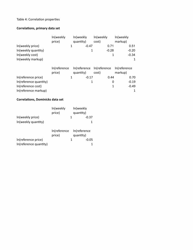
for volatile demand shocks. Second, the correlation between log(at) and log(bt)

is positive (0:7). This positive correlation helps the model match the negative

unconditional correlation between prices and quantities, reported in Table 4, while

allowing for volatile demand. Third, and most importantly, matching the data

requires an implausible pattern of comovement between at and Ct. In at least 40

percent of our observations the same price corresponds to di¤erent costs.18 To

match these observations, the change in at must exactly o¤set the change in Ct.

Although possible, this pattern of shocks strikes us as incredible.

A similar argument applies to Dixit-Stiglitz demand with stochastic elasticity

of substitution between goods. This speci�cation generates variability in markups.

However, it requires that in 40 percent of the observations shocks to the elasticity

of substitution exactly o¤set movements in marginal cost in order to rationalize a

constant price.

18This statistic is computed as follows. For each good we identify the modal price and costover the three-year sample period. We then compute the fraction of weeks in which the price isequal to the modal price but the cost is not equal to the modal cost. This calculation provides alower bound on the percentage of weeks in which the same price corresponds to di¤erent costs.

24

Menu cost models Standard menu cost models have three shortcomings with

respect to our data. First, Table 2 documents that prices are more volatile than

marginal cost, whether we work with levels or growth rates. However, calibrated

versions of menu cost models imply that prices are less volatile than marginal

cost. For example, Golosov and Lucas�(2006) model implies that the uncondi-

tional standard deviation of cost changes are 40 percent more volatile than the

unconditional standard deviation of price changes. A similar pattern obtains in

Burstein and Hellwig�s (2007) model, which incorporates demand shocks into the

Golosov-Lucas framework. The unconditional standard deviation of cost changes

is twice as large as the unconditional standard deviation of price changes in the

Burstein-Hellwig model.19 Second, we need an incredible con�guration of cost

and demand shocks to explain why �rms return often to an old (reference) price.

Third, as we discuss in Section 8, it is di¢ cult for menu cost models to match

both the frequency of weekly price changes and the frequency of reference price

changes.

Kehoe and Midrigan (2007) make progress on the second shortcoming by as-

suming that �rms set two kinds of prices, �regular�prices and �sales�prices. Sales

prices are temporary price reductions. After a sale is over the price returns to the

�regular�price. Kehoe and Midrigan assume that the menu cost associated with

a sales price change is lower than the menu cost associated with a regular price

change. It remains an open question whether such a model can rationalize the

fact that prices, both weekly and reference, are more volatile than marginal cost.

19We thank Ariel Burstein for computing the volatility of prices and costs in the Golosov-Lucasmodel and in the Burstein-Hellwig model.

25

Calvo models Perhaps the most widely used pricing model in macroeconomics

is the one associated with Calvo (1983).20 An obvious failing of the standard

Calvo (1983) pricing model is that it is inconsistent with the selection e¤ects that

we document in Figures 8-10. The Calvo model assumes that the probability of

a price change is constant. In fact, we �nd that the probability of a reference

price change is increasing in the deviation of the hypothetical markup from its

unconditional mean. It also remains an open question whether standard Calvo

pricing models are useful to understand data sets like ours in which prices are

more volatile than costs.

8. Are reference prices useful for macroeconomists?

In this section we consider a simple partial-equilibriummodel that accounts for the

key features of the data that we document in Sections 3 and 4. In this model mon-

etary policy shocks have important real e¤ects even though weekly prices change

very frequently. We use this model to illustrate the sense in which the frequency

of reference price changes can be a useful statistic to guide macroeconomists.

In our model the �rm chooses a �price plan�which consists of a small set of

prices, .21 The �rm can move between prices in this set without incurring any

cost, i.e. there are no menu costs of changing between prices in . The key friction

is that there is a �xed cost, �, of changing the price plan.

The �rm faces the following demand and cost functions:

Qt = �tP��tt ,

Ct = �1=�t ctQt,

20See, for example, Rotemberg and Woodford (1997), Gali and Gertler (1999), Smets andWouters (2003), and Christiano, Eichenbaum, and Evans (2005).21See Burstein (2006) for a di¤erent formulation of price plans in which �rms choose a deter-

ministic price sequence.

26

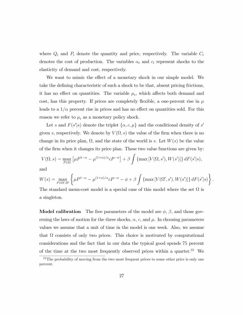
where Qt and Pt denote the quantity and price, respectively. The variable Ct

denotes the cost of production. The variables �t and ct represent shocks to the

elasticity of demand and cost, respectively.

We want to mimic the e¤ect of a monetary shock in our simple model. We

take the de�ning characteristic of such a shock to be that, absent pricing frictions,

it has no e¤ect on quantities. The variable �t, which a¤ects both demand and

cost, has this property. If prices are completely �exible, a one-percent rise in �

leads to a 1=� percent rise in prices and has no e¤ect on quantities sold. For this

reason we refer to �t as a monetary policy shock.

Let s and F (s0js) denote the triplet f�; c; �g and the conditional density of s0

given s, respectively. We denote by V (; s) the value of the �rm when there is no

change in its price plan, , and the state of the world is s. Let W (s) be the value

of the �rm when it changes its price plan. These two value functions are given by:

V (; s) = maxP2

��P 1�� � �(1+�)=�cP��

�+ �

Zfmax [V (; s0);W (s0)]g dF (s0js),

and

W (s) = maxP20;0

��P 1�� � �(1+�)=�cP�� � �+ �

Zfmax [V (0; s0);W (s0)]g dF (s0js)

�.

The standard menu-cost model is a special case of this model where the set is

a singleton.

Model calibration The free parameters of the model are �, �, and those gov-

erning the laws of motion for the three shocks, �, c, and �. In choosing parameters

values we assume that a unit of time in the model is one week. Also, we assume

that consists of only two prices. This choice is motivated by computational

considerations and the fact that in our data the typical good spends 75 percent

of the time at the two most frequently observed prices within a quarter.22 We22The probability of moving from the two most frequent prices to some other price is only one

percent.

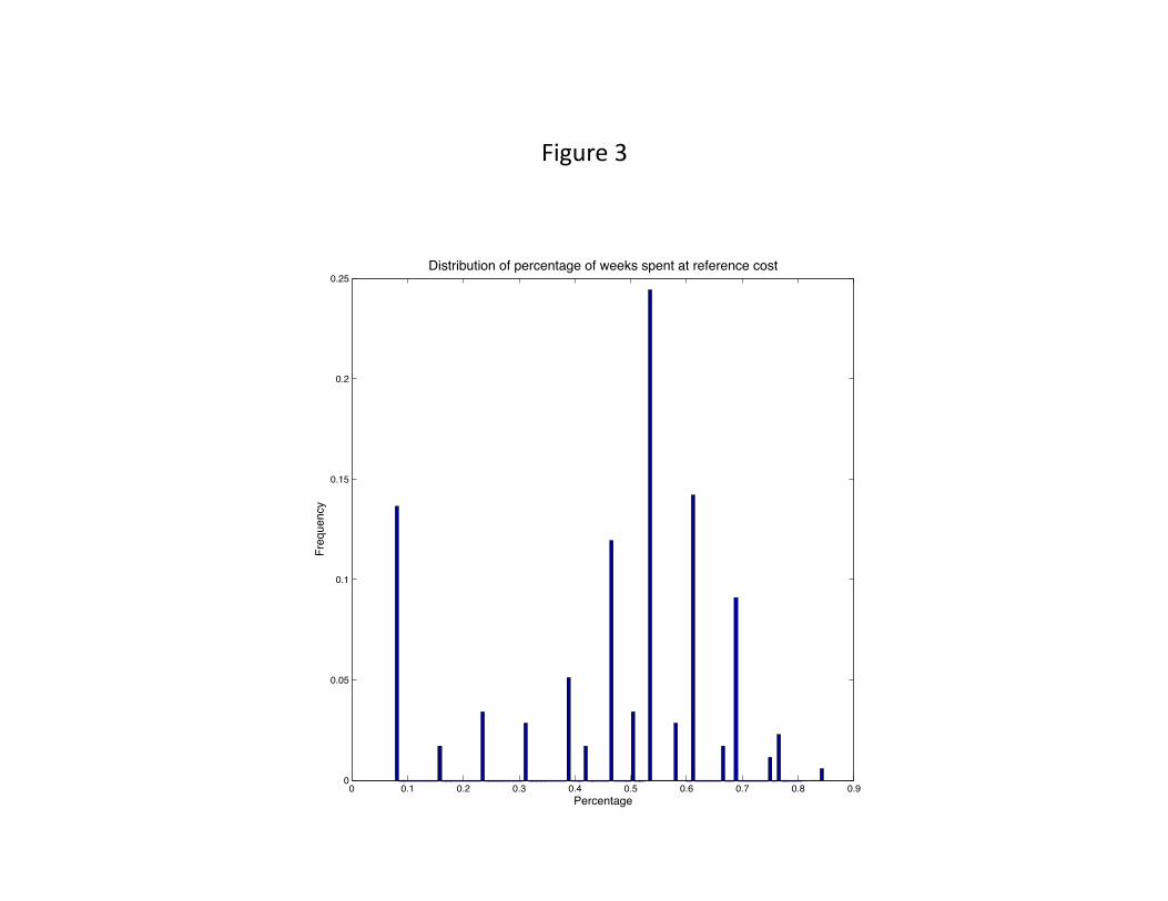
27

then choose the parameters of the model to match, as closely as possible, the mo-

ments of the data listed in Table 5. We compute the frequency of reference price

changes using the same algorithm that we use in our empirical work. Speci�cally,

we simulate the model and calculate the reference price as the modal price per

quarter.

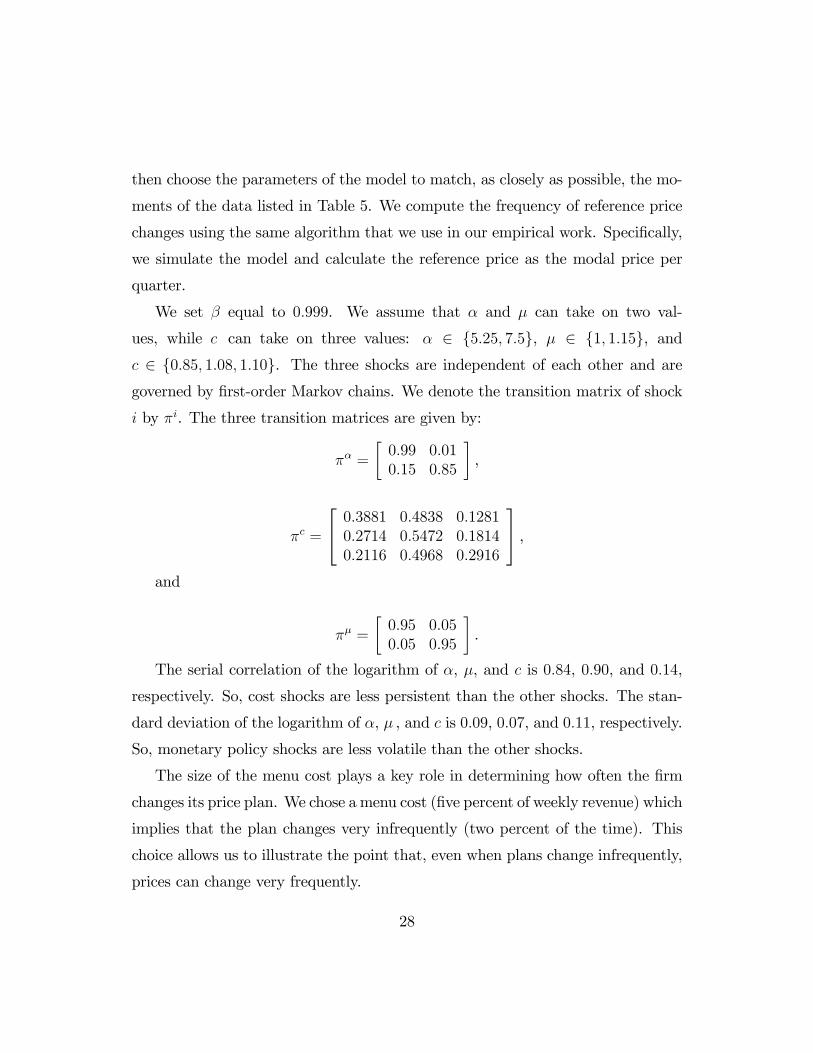
We set � equal to 0:999. We assume that � and � can take on two val-

ues, while c can take on three values: � 2 f5:25; 7:5g, � 2 f1; 1:15g, andc 2 f0:85; 1:08; 1:10g. The three shocks are independent of each other and aregoverned by �rst-order Markov chains. We denote the transition matrix of shock

i by �i. The three transition matrices are given by:

�� =

�0:990:15

0:010:85

�,

�c =

24 0:38810:27140:2116

0:48380:54720:4968

0:12810:18140:2916

35 ,and

�� =

�0:950:05

0:050:95

�.

The serial correlation of the logarithm of �, �, and c is 0:84, 0:90, and 0:14,

respectively. So, cost shocks are less persistent than the other shocks. The stan-

dard deviation of the logarithm of �, � , and c is 0:09, 0:07, and 0:11, respectively.

So, monetary policy shocks are less volatile than the other shocks.

The size of the menu cost plays a key role in determining how often the �rm

changes its price plan. We chose a menu cost (�ve percent of weekly revenue) which

implies that the plan changes very infrequently (two percent of the time). This

choice allows us to illustrate the point that, even when plans change infrequently,

prices can change very frequently.

28

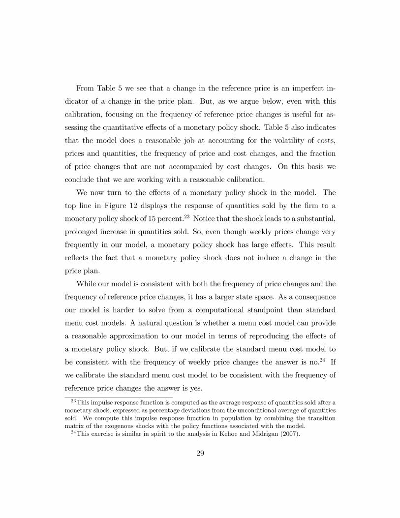
From Table 5 we see that a change in the reference price is an imperfect in-

dicator of a change in the price plan. But, as we argue below, even with this

calibration, focusing on the frequency of reference price changes is useful for as-

sessing the quantitative e¤ects of a monetary policy shock. Table 5 also indicates

that the model does a reasonable job at accounting for the volatility of costs,

prices and quantities, the frequency of price and cost changes, and the fraction

of price changes that are not accompanied by cost changes. On this basis we

conclude that we are working with a reasonable calibration.

We now turn to the e¤ects of a monetary policy shock in the model. The

top line in Figure 12 displays the response of quantities sold by the �rm to a

monetary policy shock of 15 percent.23 Notice that the shock leads to a substantial,

prolonged increase in quantities sold. So, even though weekly prices change very

frequently in our model, a monetary policy shock has large e¤ects. This result

re�ects the fact that a monetary policy shock does not induce a change in the

price plan.

While our model is consistent with both the frequency of price changes and the

frequency of reference price changes, it has a larger state space. As a consequence

our model is harder to solve from a computational standpoint than standard

menu cost models. A natural question is whether a menu cost model can provide

a reasonable approximation to our model in terms of reproducing the e¤ects of

a monetary policy shock. But, if we calibrate the standard menu cost model to

be consistent with the frequency of weekly price changes the answer is no.24 If

we calibrate the standard menu cost model to be consistent with the frequency of

reference price changes the answer is yes.

23This impulse response function is computed as the average response of quantities sold after amonetary shock, expressed as percentage deviations from the unconditional average of quantitiessold. We compute this impulse response function in population by combining the transitionmatrix of the exogenous shocks with the policy functions associated with the model.24This exercise is similar in spirit to the analysis in Kehoe and Midrigan (2007).

29

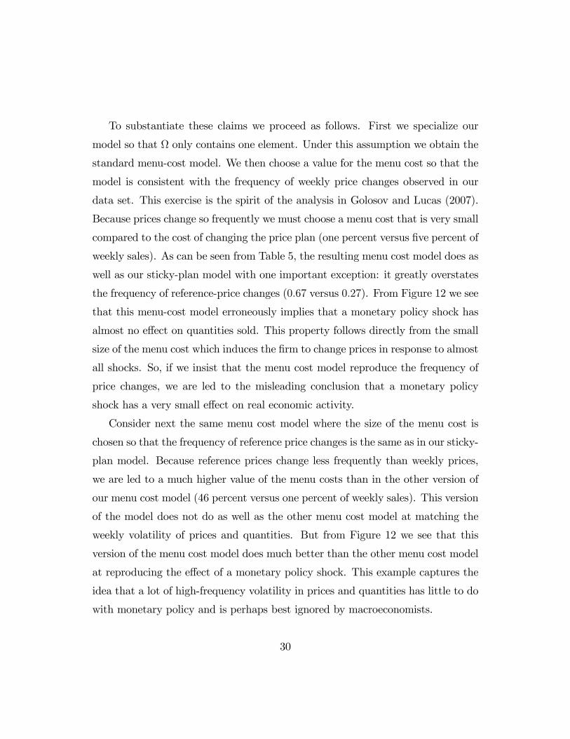
To substantiate these claims we proceed as follows. First we specialize our

model so that only contains one element. Under this assumption we obtain the

standard menu-cost model. We then choose a value for the menu cost so that the

model is consistent with the frequency of weekly price changes observed in our

data set. This exercise is the spirit of the analysis in Golosov and Lucas (2007).

Because prices change so frequently we must choose a menu cost that is very small

compared to the cost of changing the price plan (one percent versus �ve percent of

weekly sales). As can be seen from Table 5, the resulting menu cost model does as

well as our sticky-plan model with one important exception: it greatly overstates

the frequency of reference-price changes (0:67 versus 0:27). From Figure 12 we see

that this menu-cost model erroneously implies that a monetary policy shock has

almost no e¤ect on quantities sold. This property follows directly from the small

size of the menu cost which induces the �rm to change prices in response to almost

all shocks. So, if we insist that the menu cost model reproduce the frequency of

price changes, we are led to the misleading conclusion that a monetary policy

shock has a very small e¤ect on real economic activity.

Consider next the same menu cost model where the size of the menu cost is

chosen so that the frequency of reference price changes is the same as in our sticky-

plan model. Because reference prices change less frequently than weekly prices,

we are led to a much higher value of the menu costs than in the other version of

our menu cost model (46 percent versus one percent of weekly sales). This version

of the model does not do as well as the other menu cost model at matching the

weekly volatility of prices and quantities. But from Figure 12 we see that this

version of the menu cost model does much better than the other menu cost model

at reproducing the e¤ect of a monetary policy shock. This example captures the

idea that a lot of high-frequency volatility in prices and quantities has little to do

with monetary policy and is perhaps best ignored by macroeconomists.

30

9. Conclusion

We present evidence that is consistent with the view that nominal rigidities are

important. However, these rigidities do not take the form of sticky prices, i.e.

prices that remain constant over time. Instead, nominal rigidities take the form

of inertia in reference prices and costs. Weekly prices and costs �uctuate around

reference values which tend to remain constant over extended periods of time.

Reference prices are particularly inertial and have an average duration of roughly

one year. So, nominal rigidities are present in our data, even though prices and

cost change very frequently, roughly once every two weeks. We document the

relation between prices and costs and argue that reference prices and costs are

useful statistics for macroeconomic analysis.

31

References

[1] Altig, David, Lawrence Christiano, Martin Eichenbaum, and Jesper Linde

�Firm-speci�c capital, nominal rigidities and the business cycle,� mimeo,

Northwestern University, 2004.

[2] Arigaa, Kenn, Kenji Matsuib, Makoto Watanabeb �Hot and spicy: ups and

downs on the price �oor and ceiling at Japanese supermarkets,�mimeo, Grad-

uate School of Economics, Kyoto University, 2001.

[3] Bils, Mark, and Peter J. Klenow. �Some evidence on the importance of sticky

prices,�Journal of Political Economy 112 (October): 947�85, 2004.

[4] Blinder, Alan S., Elie R. D. Canetti, David E. Lebow, and Jeremy B. Rudd

�Asking about prices: a new approach to understanding price stickiness,�

New York: Sage Found, 1998.

[5] Burstein, Ariel �In�ation and output dynamics with state dependent pricing

decisions,�Journal of Monetary Economics, 53: 7, pp. 1235-1257, October

2006.

[6] Burstein, Ariel and Christian Hellwig, �Prices and market shares in a menu

cost model,�mimeo, UCLA, 2007.

[7] Calvo, Guillermo, A. �Staggered prices in a utility-maximizing framework,�

Journal of Monetary Economics 12 (September): 383�98, 1983.

[8] Campbell, Je¤rey and Benjamin Eden �Rigid Prices: Evidence from U.S.

Scanner Data,�mimeo, Vanderbilt University, October, 2005.

32

[9] Chevalier, Judith A., Anil Kashyap and Peter E. Rossi �Why don�t prices

rise during periods of peak demand? Evidence from scanner data,�American

Economic Review, 93 (1), pp. 15-37, 2003.

[10] Christiano, Lawrence, Eichenbaum, Martin and Charles Evans, �Nominal

rigidities and the dynamic e¤ects of a shock to monetary policy,�Journal of

Political Economy, 113 (1), 1-45, 2005.

[11] Gali, Jordi, and Mark Gertler, �In�ation dynamics: a structural econometric

analysis,�Journal of Monetary Economics, 1999, 44, pp. 195-222.

[12] Goldberg, Pinelopi K. and Rebecca Hellerstein �A Framework for Identifying

the Sources of Local-currency Price Stability with an Empirical Application,�

National Bureau of Economic Research, Working Paper 13183, June 2007.

[13] Golosov, Mikhail, and Robert E. Lucas, Jr. �Menu costs and Phillips curves,�

Journal of Political Economy, 115: 171-199, 2007.

[14] Hosken, Daniel and David Rei¤en �Patterns of retail price variation,�The

RAND Journal of Economics, 35, 1: 128-146, 2004.

[15] Kehoe, Patrick and Virgiliu Midrigan �Sales and the real e¤ects of monetary

policy,�mimeo, University of Minnesota, 2007.

[16] Kimball, Miles, �The quantitative analytics of the basic neomonetarist

model,� Journal of Money, Credit, and Banking, 27(4), Part 2, pp. 1241-

1277, 1995.

[17] Maratou, Laoura �Bargaining power impact on o¤-invoice trade promotions

in U.S. grocery retailing,�mimeo, Cornell University, 2006.

33

[18] Maratou, Laoura, Miguel Gómez, and David Just �Market power impact on

o¤-invoice trade promotions in US grocery retailing,�mimeo, Cornell Uni-

versity, 2004.

[19] Midrigan, Virgiliu �Menu costs, multiproduct �rms, and aggregate �uctua-

tions,�Mimeo, Federal Reserve Bank of Minneapolis, 2006.

[20] Nakamura, Emi, and Jón Steinsson �Five facts about prices: A reevaluation

of menu cost models,�Mimeo, Harvard University, 2007.

[21] Pesendorfer, Martin �Retail Sales: A Study of Pricing Behavior in Super-

markets,�Journal of Business, 75: 33-66, 2002.

[22] Rotemberg, Julio J. and Michael Woodford, �An optimization-based econo-

metric framework for the evaluation of monetary policy,�National Bureau of

Economic Research Macroeconomics Annual, 1997.

[23] Slade, Margaret E. �Optimal Pricing with Costly Adjustment: Evidence from

Retail-Grocery Prices,�Review of Economic Studies 65, 87-107, 1998.

[24] Smets, Frank and Raf Wouters �An estimated dynamic stochastic general

equilibrium model of the Euro area,�Journal of the European Economic As-

sociation, September 2003, Vol. 1, No. 5, 1123-1175.

[25] Warner, Elizabeth and Robert Barsky �The timing and magnitude of re-

tail store markdowns: evidence from weekends and holidays,�The Quarterly

Journal of Economics, 321-351, 1995.

34

!"#$%&'(&)"*+,&*-".*.,*&

/0+1"02&

3"-"&*%-

451+6+,7*&

3"-"&*%-

!"#$%&#'"(#(%#

80",.56&59&:%%7*&*;%6-&"-&-<%&0%9%0%6,%&;0+,% =>?@ =>AA

80",.56&59&:%%7*&*;%6-&"-&-<%&0%9%0%6,%&,5*- =>BC 6>">

80",.56&59&DE"0-%0*&+6&:<+,<&:%%7$2&;0+,%*&"0%&,56*-"6-&950&-<%&:<5$%&DE"0-%0 =>'' =>'F

80",.56&59&DE"0-%0*&+6&:<+,<&:%%7$2&,5*-&+*&,56*-"6-&950&-<%&:<5$%&DE"0-%0 =>=? 6>">

80",.56&59&656G0%9%0%6,%&;0+,%*&-<"-&"0%&"#5H%&0%9%0%6,%&;0+,%*II 0.21 =>J=

80",.56&59&;0+,%&,<"6K%*&-<"-&"0%&9051&"&656G0%9%0%6,%&;0+,%&-5&"&0%9%0%6,%&;0+,% =>@F =>C'

80",.56&59&,5*-&,<"6K%*&-<"-&"0%&9051&"&656G0%9%0%6,%&,5*-&-5&"&0%9%0%6,%&,5*- =>@B 6>">

80",.56&59&DE"6..%*&*5$3&"-&0%9%0%6,%&;0+,%* =>CF =>??

80",.56&59&0%H%6E%&,5$$%,-%3&"-&0%9%0%6,%&;0+,%* 0.54 =>?L

/05#"#+$+-2&59&:%%7$2&;0+,%&,<"6K+6K&:<%6&:%%7$2&,5*-&35%*&65-&,<"6K% =>=J 6>">

/05#"#+$+-2&59&0%9%0%6,%&;0+,%&,<"6K+6K&:<%6&0%9%0%6,%&,5*-&35%*&65-&,<"6K% =>'B 6>">

IIM51;E-%3&5E-&59&-<%&-5-"$&:%%7*&+6&:<+,<&-<%&:%%7$2&;0+,%&+*&3+N%0%6-&9051&-<%&0%9%0%6,%&;0+,%>

!"#$%&'(&)*$"+$,-.&/0*/%0+%1

20,3"0.&

4"-"&1%-

5*3,6,781&

4"-"&1%-

9!:;5:<5&5=)>:!>?;&?@&A=)=A9

!"#$%#&%'%()*#+,$',-'./#$++(0

A*BCD%%8$.&EF"6+-.G& 0.53 HIJK

A*BCEF"6++%1&1*$4&"-&0%L%0%67%&/0,7%G& 0.42 HIMN

A*BCEF"6++%1&1*$4&"-&6*6O0%L%0%67%&/0,7%1G& 0.43 HIM'

!"#$%#&%'%()*#+,$',-'1&*2(0

A*BCD%%8$.&/0,7%G& 0.14 HINN

A*BC0%L%0%67%&/0,7%G& 0.08 HIHK

A*BCD%%8$.&/0,7%GP&7*64,+*6"$&*6&D%%8$.&/0,7%&7Q"6B% 0.15 HINR

A*BC0%L%0%67%&/0,7%GP&7*64,+*6"$&*6&0%L%0%67%&/0,7%&7Q"6B% 0.10 HIHK

!"#$%#&%'%()*#+,$',-'2,0"0

A*BCD%%8$.&7*1-G 0.12 6I"I

A*BC0%L%0%67%&7*1-G 0.07 6I"I

A*BCD%%8$.&7*1-GP&7*64,+*6"$&*6&7*1-&7Q"6B% 0.13 6I"I

A*BC0%L%0%67%&7*1-GP&7*64,+*6"$&*6&7*1-&7Q"6B% 0.08 6I"I

!"#$%#&%'%()*#+,$',-'1&*2(03!"#$%#&%'%()*#+,$',-'2,0"04

S%%8$.&/0,7%1TD%%8$.&7*1-1 1.08 6I"I

<%L%0%67%&/0,7%1T0%L%0%67%&7*1-1 1.15 6I"I

S%%8$.&/0,7%1P&7*64,+*6"$&*6&/0,7%&7Q"6B%1TD%%8$.&7*1-&7*64,+*6"$&*6&7*1-&7Q"6B% 1.08 6I"I

<%L%0%67%&/0,7%P&7*64,+*6"$&*6&/0,7%&7Q"6B%1T0%L%0%67%&7*1-P&7*64,+*6"$&*6&7*1-&7Q"6B%1 1.17 6I"I

!"#$%#&%'%()*#+,$',-'5#&6/1

A*BCD%%8$.&3"08F/G& HINN 6I"I

A*BC0%L%0%67%&3"08F/G& 0.09 6I"I

9!:;5:<5&5=)>:!>?;&?@&UV:;W=9

!"#$%#&%'%()*#+,$',-'1&*2(0

A*B&7Q"6B%1&,6&D%%8$.&/0,7%1 0.14 HIHX

A*B&7Q"6B%1&,6&0%L%0%67%&/0,7%1 0.08 HIHM

A*B&7Q"6B%1&,6&D%%8$.&/0,7%1P&7*64,+*6"$&*6&/0,7%&7Q"6B% 0.20 HINX

A*B&7Q"6B%1&,6&0%L%0%67%&/0,7%1P&7*64,+*6"$&*6&/0,7%&7Q"6B% 0.14 HIHK

!"#$%#&%'%()*#+,$',-'2,0"0

A*B&7Q"6B%1&,6&D%%8$.&7*1- 0.11 6I"I

A*B&7Q"6B%1&,6&0%L%0%67%&7*1- 0.06 6I"I

A*B&7Q"6B%1&,6&D%%8$.&7*1-P&7*64,+*6"$&*6&7*1-&7Q"6B% 0.15 6I"I

A*B&7Q"6B%1&,6&0%L%0%67%&7*1-P&7*64,+*6"$&*6&7*1-&7Q"6B% 0.09 6I"I

!"#$%#&%'%()*#+,$',-'1&*2(03!"#$%#&%'%()*#+,$',-'2,0"04

S%%8$.&B0*D-Q&0"-%&*L&/0,7%1TD%%8$.&B0*D-Q&0"-%&*L&7*1-1 1.10 6I"I

<%L%0%67%&B0*D-Q&0"-%&*L&/0,7%1TB0*D-Q&0"-%&*L&7*1-1 1.13 6I"I

S%%8$.&B0*D-Q&0"-%&*L&/0,7%P&7*64,+*6"$&*6&/0,7%&7Q"6B%1TD%%8$.&B0*D-Q&0"-%&*L&7*1-P&7*64,+*6"$&*6&7*1-&

7Q"6B% 1.20 6I"I

W0*D-Q&0"-%&*L&0%L%0%67%&/0,7%1&7*64,+*6"$&*6&/0,7%&7Q"6B%1TB0*D-Q&0"-%&*L&0%L%0%67%&7*1-1P&7*64,+*6"$&

*6&7*1-&7Q"6B%1 1.25 6I"I

Y;*-%(&-Q%&3%4,"6&*L&-Q%&0"+*&*L&1-"64"04&4%Z,"+*61&,1&6*-&-Q%&0"+*&*L&-Q%&3%4,"6&1-"64"04&4%Z,"+*61I

!"#$%&'(&)%*+,+-%./%&0*10%*2%+

)*,3"*4&

5"-"&+%-

613,.,/7+&

5"-"&+%-

!"#$%&'%"(#()%*$%

)*1#"#,$,-4&18&"&9%%7$4&0*,/%&/:".;% <=>' <=?>

@30$,%5&9%%7$4&0*,/%&5A*"21.&B,.&CA"*-%*+D <=EF <='?

)*1#"#,$,-4&18&*%8%*%./%&0*,/%&/:".;%+ <=?G <=''

@30$,%5&*%8%*%./%&0*,/%&5A*"21.&B,.&CA"*-%*+D '=G< '=<'

+,()&'%"(#()%*$%

)*1#"#,$,-4&18&9%%7$4&/1+-&/:".;%+ <=>H .="=

@30$,%5&9%%7$4&/1+-&5A*"21.&B,.&CA"*-%*+D <=EI .="=

)*1#"#,$,-4&18&*%8%*%./%&/1+-&/:".;%+ <=>J .="=

@30$,%5&*%8%*%./%&/1+-&5A*"21.&B,.&CA"*-%*+D ?=?? .="=

!"#$%&'(&)*++%$",*-&.+*.%+,%/

!"##$%&'"()*+,#-.&#/+0&1&+)$1

$-01%%2$3&

.+45%6

$-01%%2$3&

78"-,936

$-01%%2$3&

5*/96

$-01%%2$3&

:"+28.6

$-01%%2$3&.+45%6 ; -0.47 0.71 0.51

$-01%%2$3&78"-,936 ; -0.28 -0.20

$-01%%2$3&5*/96 ; -0.34

$-01%%2$3&:"+28.6 ;

$-0+%<%+%-5%&

.+45%6

$-0+%<%+%-5%&

78"-,936

$-0+%<%+%-5%&

5*/96

$-0+%<%+%-5%&

:"+28.6

$-0+%<%+%-5%&.+45%6 ; =>?;@ >?'' >?@>

$-0+%<%+%-5%&78"-,936 ; > =>?;A

$-0+%<%+%-5%&5*/96 ; =>?'A

$-0+%<%+%-5%&:"+28.6 ;

!"##$%&'"()*+2".-(-34)+0&1&+)$1

$-01%%2$3&

.+45%6

$-01%%2$3&

78"-,936

$-01%%2$3&.+45%6 ; =>?B@

$-01%%2$3&78"-,936 ;

$-0+%<%+%-5%&

.+45%6

$-0+%<%+%-5%&

78"-,936

$-0+%<%+%-5%&.+45%6 ; =>?>C

$-0+%<%+%-5%&78"-,936 ;

!"#$%&'(&)"*"&"+,&-.,%$&/*"0/01/

Data

Sticky plan

model

Menu cost

calibrated to

the frequency

of weekly price

changes

Menu cost

model calibrated

to frequency of

reference price

changes

Menu cost value as percentage of steady state cash flow 0.0525 0.0100 0.4593

Weekly cost volatility 0.120 0.112 0.113 0.112

Weekly price volatility 0.140 0.111 0.113 0.075

Weekly quantity volatility 0.530 0.600 0.599 0.416

Frequency of weekly price changes 0.430 0.375 0.402 0.155

Frequency of weekly cost changes 0.490 0.577 0.574 0.576

Frequency of reference price changes 0.270 0.268 0.670 0.269

Frequency of reference costs changes 0.450 0.634 0.628 0.635

Fraction of price changes without cost changes 0.030 0.011 0.009 0.003

Frequency of plan changes 0.023

!"#$%&'('

0 0.1 0.2 0.3 0.4 0.5 0.6 0.7 0.8 0.9 10

0.05

0.1

0.15

0.2

0.25

Distribution of percentage of weeks spent at reference price

Percentage

Fre

quency

0 0.1 0.2 0.3 0.4 0.5 0.6 0.7 0.8 0.9 10

0.005

0.01

0.015

0.02

0.025

0.03

0.035

Distribution of percentage ot total quantity sold at reference price

Percentage

Fre

quency

!"#$%&'('

0 50 100 1500

0.02

0.04

0.06

0.08

0.1

0.12

0.14

Distribution of weekly price duration

weeks

Fre

quency

0 50 100 1500

0.05

0.1

0.15

0.2

0.25

0.3

0.35

Distribution of reference price duration

weeks

Fre

quency

!"#$%&'('

0 0.1 0.2 0.3 0.4 0.5 0.6 0.7 0.8 0.90

0.05

0.1

0.15

0.2

0.25

Distribution of percentage of weeks spent at reference cost

Percentage

Fre

quency

!"#$%&'('

0 50 100 1500

0.02

0.04

0.06

0.08

0.1

0.12

0.14

0.16

Distribution of weekly cost duration

weeks

Fre

quency

0 50 100 1500

0.02

0.04

0.06

0.08

0.1

0.12

0.14

0.16

0.18

Distribution of reference cost duration

weeks

Fre

quency

!"#$%&'('

!!"# !!"!$ !!"!% !!"!& !!"!' ! !"!' !"!& !"!% !"!$ !"#!

!"!(

!"#

!"#(

!"'

!"'(

!")

!")(

*+,-+./01+23+450/56.27,68204+,01+280,9:;

<,+=:+.->

!"#$%&'('

!!"# !!"!$ ! !"!$ !"#!

!"%

!"&

!"'

()*+,-./0#01)+*,2*3

40526-+,-./07*.80+62*+9208+*:);

!!"# !!"!$ ! !"!$ !"#!

!"#

!"%

!"<

()*+,-./0%01)+*,2*3

40526-+,-./07*.80+62*+9208+*:);

!!"# !!"!$ ! !"!$ !"#!

!"#

!"%

!"<

()*+,-./0<01)+*,2*3

40526-+,-./07*.80+62*+9208+*:);

!!"# !!"!$ ! !"!$ !"#!

!"#

!"%

!"<

()*+,-./0&01)+*,2*3

40526-+,-./07*.80+62*+9208+*:);

!!"# !!"!$ ! !"!$ !"#!

!"#

!"%

()*+,-./0$01)+*,2*3

40526-+,-./07*.80+62*+9208+*:);

!!"# !!"!$ ! !"!$ !"#!

!"#

!"%

()*+,-./0'01)+*,2*3

40526-+,-./07*.80+62*+9208+*:);

!!"# !!"!$ ! !"!$ !"#!

!"#

!"%

()*+,-./0=01)+*,2*3

40526-+,-./07*.80+62*+9208+*:);

!!"# !!"!$ ! !"!$ !"#!

!"#

!"%

()*+,-./0>01)+*,2*3

40526-+,-./07*.80+62*+9208+*:);

!!"# !!"!$ ! !"!$ !"#!

!"#

!"%

()*+,-./0?01)+*,2*3

40526-+,-./07*.80+62*+9208+*:);

!!"# !!"!$ ! !"!$ !"#!

!"!$

!"#

!"#$

!"%

()*+,-./0#!01)+*,2*3

40526-+,-./07*.80+62*+9208+*:);

!!"# !!"!$ ! !"!$ !"#!

!"#

!"%

()*+,-./0##01)+*,2*3

40526-+,-./07*.80+62*+9208+*:);

!!"# !!"!$ ! !"!$ !"#!

!"!$

!"#

!"#$

!"%

()*+,-./0#%01)+*,2*3

40526-+,-./07*.80+62*+9208+*:);

0 0.1 0.2 0.3 0.4 0.5 0.6 0.7 0.8 0.9 10

0.1

0.2

0.3

0.4

0.5

0.6

0.7

0.8

0.9

1

Pro

babili

ty o

f a c

hange in the r

efe

rence p

rice

(P

)

Probability of a change in the reference cost (C)

!"#$%&'('

)'*'+,-,./('0',-/,1,23'

45'*',-6,'

!"#$%&'('

!!"# !!"!$ ! !"!$ !"# !"#$

!"%

!"%$

!"&

!"&$

!"'

!"'$

!"$

!"$$

()*+,+-.-/01*21,1)323)345316)-53157,483

(3)534/,83193:-,/-*4;1*21706*/73/-5,.1<,)=>612)*<1,:3),831<,)=>6

!!"# !!"!$ ! !"!$ !"# !"#$

!!"#

!!"!$

!

!"!$

!"#

!"#$

?3,.-@391)323)34531<,)=>61,;163)534/,83193:-,/-*412)*<1,:3),831<,)=>6A15*49-/-*4,.1*41,1)323)345316)-53157,483

(3)534/,83193:-,/-*4;1*21706*/73/-5,.1<,)=>612)*<1,:3),831<,)=>6

!"#$%&'('

)%*+,+"-"./'*0'%&0&%&12&'3%"2&'24,1#&',5','0$126*1'*0'

3&%2&1.,#&'7&8",6*1'*0'4/3*.4&62,-'9,%:$3'0%*9',8&%,#&'9,%:$3''

0*%'#**75';".4'7"<&%&1.'3%"2&'7$%,6*1'

!!"# !!"!$ ! !"!$ !"# !"#$!"%&

!"%%

!"'

!"'(

!"')

*+,-./012(23+-,.4,5

!!"# !!"!$ ! !"!$ !"# !"#$

!"6

!"6$

!"%

!"%$

*+,-./012723+-,.4,5

!!"# !!"!$ ! !"!$ !"# !"#$

!"&

!"&$

!"6

!"6$

*+,-./012)23+-,.4,5

!!"# !!"!$ ! !"!$ !"# !"#$

!"$

!"$$

!"&

!"&$

*+,-./012$23+-,.4,5

!!"# !!"!$ ! !"!$ !"# !"#$

!")

!")$

!"$

!"$$

!"&

*+,-./012&23+-,.4,5

!!"# !!"!$ ! !"!$ !"# !"#$

!"7

!")

!"$

*+,-./012623+-,.4,5

!!"# !!"!$ ! !"!$ !"# !"#$

!"7

!")

!"$

*+,-./012%23+-,.4,5

!!"# !!"!$ ! !"!$ !"# !"#$

!"(

!"7

!")

*+,-./012'23+-,.4,5

!!"# !!"!$ ! !"!$ !"# !"#$

!"#

!"(

!"7

*+,-./012#!23+-,.4,5

!!"# !!"!$ ! !"!$ !"# !"#$

!"!$

!"#

!"#$

!"(

!"($

*+,-./012##23+-,.4,5

!"#$%&'()'

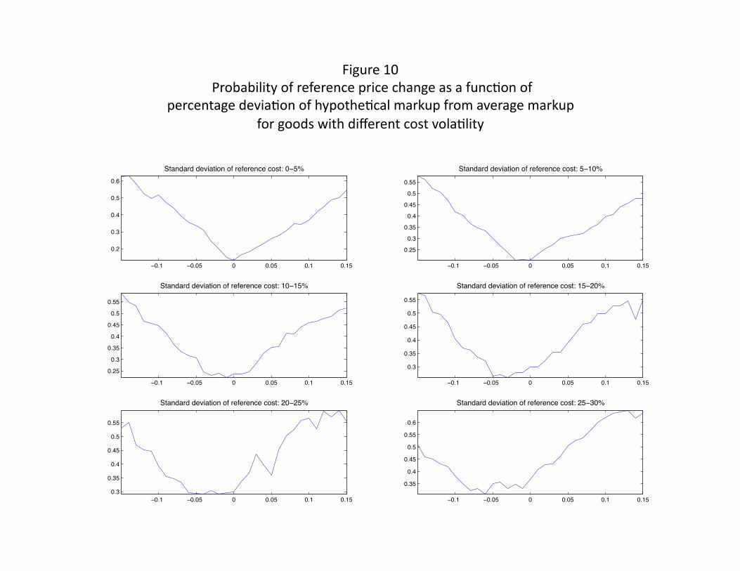
'*%+,-,"."/0'+1'%&1&%&23&'4%"3&'35-2#&'-6'-'1$237+2'+1'

4&%3&2/-#&'8&9"-7+2'+1'504+/5&73-.':-%;$4'1%+:'-9&%-#&':-%;$4''

1+%'#++86'<"/5'8"=&%&2/'3+6/'9+.-7."/0'

!!"# !!"!$ ! !"!$ !"# !"#$

!"%

!"&

!"'

!"$

!"(

)*+,-+.-/-012+*23,/34/.040.0,50/536*7/!!$8

!!"# !!"!$ ! !"!$ !"# !"#$

!"%$

!"&

!"&$

!"'

!"'$

!"$

!"$$

)*+,-+.-/-012+*23,/34/.040.0,50/536*7/$!#!8

!!"# !!"!$ ! !"!$ !"# !"#$

!"%$

!"&

!"&$

!"'

!"'$

!"$

!"$$

)*+,-+.-/-012+*23,/34/.040.0,50/536*7/#!!#$8

!!"# !!"!$ ! !"!$ !"# !"#$

!"&

!"&$

!"'

!"'$

!"$

!"$$

)*+,-+.-/-012+*23,/34/.040.0,50/536*7/#$!%!8

!!"# !!"!$ ! !"!$ !"# !"#$

!"&

!"&$

!"'

!"'$

!"$

!"$$

)*+,-+.-/-012+*23,/34/.040.0,50/536*7/%!!%$8

!!"# !!"!$ ! !"!$ !"# !"#$

!"&$

!"'

!"'$

!"$

!"$$

!"(

)*+,-+.-/-012+*23,/34/.040.0,50/536*7/%$!&!8

!"#$%&'(('

!!" !# !$ !% !& !' !( !) !* !! "

!"+"%

!"+"&

!"+"'

!"+"(

!"+")

!"+"*

!"+"!

"

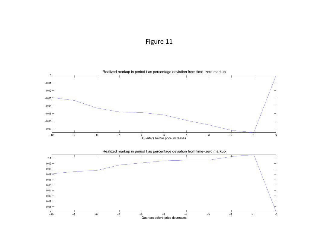
,-./01-234.567830938-50:23;3.<38-5=-9;.>-32-?0.;0:93@5:43;04-!1-5:34.5678

A7.5;-5<3B-@:5-3850=-309=5-.<-<

!!" !# !$ !% !& !' !( !) !* !! ""

"+"!

"+"*

"+")

"+"(

"+"'

"+"&

"+"%

"+"$

"+"#

"+!

,-./01-234.567830938-50:23;3.<38-5=-9;.>-32-?0.;0:93@5:43;04-!1-5:34.5678

A7.5;-5<3B-@:5-3850=-32-=5-.<-<

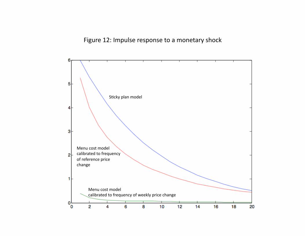
!"#$%&'()*'+,-$./&'%&/-01/&'20'3',01&23%4'/5067'

89674'-.31',0:&.'

;&1$'60/2',0:&.'

63."<%32&:'20'=%&>$&164'

0='%&=&%&16&'-%"6&'

6531#&'

;&1$'60/2',0:&.'

63."<%32&:'20'=%&>$&164'0='?&&7.4'-%"6&'6531#&'