Nominal Rigidities and the Dynamic Effects of a Shock to ...faculty.wcas.northwestern.edu/~lchrist/research/modeling/... · Nominal Rigidities and the Dynamic ... see Sims (1998),

1

[Journal of Political Economy, 2005, vol. 113, no. 1]� 2005 by The University of Chicago. All rights reserved. 0022-3808/2005/11301-0003$10.00

Nominal Rigidities and the Dynamic Effects of a

Shock to Monetary Policy

Lawrence J. Christiano and Martin EichenbaumNorthwestern University, National Bureau of Economic Research, and Federal Reserve Bank ofChicago

Charles L. EvansFederal Reserve Bank of Chicago

We present a model embodying moderate amounts of nominal rigid-ities that accounts for the observed inertia in inflation and persistencein output. The key features of our model are those that prevent asharp rise in marginal costs after an expansionary shock to monetarypolicy. Of these features, the most important are staggered wage con-tracts that have an average duration of three quarters and variablecapital utilization.

I. Introduction

This paper seeks to understand the observed inertial behavior of infla-tion and persistence in aggregate quantities. To this end, we formulateand estimate a dynamic, general equilibrium model that incorporatesstaggered wage and price contracts. We use our model to investigatethe mix of frictions that can account for the evidence of inertia andpersistence. For this exercise to be well defined, we must characterize

The first two authors are grateful for the financial support of a National Science Foun-dation grant to the National Bureau of Economic Research. We would like to acknowledgehelpful comments from Lars Hansen and Mark Watson. We particularly want to thankLevon Barseghyan for his superb research assistance, as well as his insightful commentson various drafts of the paper. This paper does not necessarily reflect the views of theFederal Reserve Bank of Chicago or the Federal Reserve System.

2 journal of political economy

inertia and persistence precisely. We do so using estimates of the dy-namic response of inflation and aggregate variables to a monetary policyshock. With this characterization, the question we ask reduces to thefollowing: Can models with moderate degrees of nominal rigidities gen-erate inertial inflation and persistent output movements in response toa monetary policy shock?1 Our answer to this question is yes.

The model that we construct has two key features. First, it embedsCalvo-style nominal price and wage contracts. Second, the real side ofthe model incorporates four departures from the standard textbook,one-sector dynamic stochastic growth model. These departures are mo-tivated by recent research on the determinants of consumption, assetprices, investment, and productivity. The specific departures that weinclude are habit formation in preferences for consumption, adjustmentcosts in investment, and variable capital utilization. In addition, we as-sume that firms must borrow working capital to finance their wage bill.

Our key findings are as follows. First, the average duration of priceand wage contracts in the estimated model is roughly two and threequarters, respectively. Despite the modest nature of these nominal ri-gidities, the model does a very good job of accounting quantitativelyfor the estimated response of the U.S. economy to a policy shock. Inaddition to reproducing the dynamic response of inflation and output,the model also accounts for the delayed, hump-shaped response in con-sumption, investment, profits, and productivity and the weak responseof the real wage.2 Second, the critical nominal friction in our model iswage contracts, not price contracts. A version of the model with onlynominal wage rigidities does almost as well as the estimated model. Incontrast, with only nominal price rigidities, the model performs verypoorly. Consistent with existing results in the literature, the version ofthe model with only price rigidities cannot generate persistent move-ments in output unless we assume price contracts of extremely longduration. The model with only nominal wage rigidities does not havethis problem.

Third, we document how inference about nominal rigidities variesacross different specifications of the real side of our model.3 Estimated

1 This question is the focus of a large and growing literature. See, e.g., Rotemberg andWoodford (1999), Chari, Kehoe, and McGrattan (2000), Mankiw (2001), and the refer-ences therein.

2 In related work, Sbordone (2000) argues that, when aggregate real variables are takenas given, a model with staggered wages and prices does well at accounting for the time-series properties of wages and prices. See also Ambler, Guay, and Phaneuf (1999) andHuang and Liu (2002) for interesting work on the role of wage contracts.

3 For early discussions about the impact of real frictions on the effects of nominalrigidities, see Blanchard and Fischer (1989), Ball and Romer (1990), and Romer (1996).For more recent quantitative discussions, see Sims (1998), McCallum and Nelson (1999),Chari et al. (2000), Edge (2000), and Fuhrer (2000).

nominal rigidities 3

versions of the model that do not incorporate our departures from thestandard growth model imply implausibly long price and wage contracts.Fourth, we find that if one wants to generate inertia in inflation andpersistence in output in a model while imposing only moderate wageand price stickiness, then it is crucial to allow for variable capital util-ization. To understand why this feature is so important, note that in ourmodel, firms set prices as a markup over marginal costs. The majorcomponents of marginal costs are wages and the rental rate of capital.By allowing the services of capital to increase after a positive monetarypolicy shock, variable capital utilization helps dampen the large rise inthe rental rate of capital that would otherwise occur. This in turn damp-ens the rise in marginal costs and, hence, prices. The resulting inertiain inflation implies that the rise in nominal spending that occurs aftera positive monetary policy shock produces a persistent rise in real out-put. Similar intuition explains why sticky wages play a critical role inallowing our model to explain inflation inertia and output persistence.It also explains why our assumption about working capital plays a usefulrole: Other things equal, a decline in the interest rate lowers marginalcosts.

Fifth, although investment adjustment costs and habit formation donot play a central role with respect to inflation inertia and output per-sistence, they do play a critical role in accounting for the dynamics ofother variables. Sixth, the major role played by the working capitalchannel is to reduce the model’s reliance on sticky prices. Specifically,if we estimate a version of the model that does not allow for workingcapital, the average duration of price contracts increases dramatically.Finally, we find that our model embodies strong internal propagationmechanisms. The impact of a monetary policy shock on aggregate ac-tivity continues to grow and persist even beyond the time at which thetypical contract that was in place at the time of the shock has beenreoptimized. In addition, the effects on real variables persist well beyondthe effects of the shock on the interest rate and the growth rate ofmoney.

We pursue a particular limited information econometric strategy toestimate and evaluate our model. To implement this strategy we firstestimate the impulse response of eight key macroeconomic variables toa monetary policy shock, using an identified vector autoregression(VAR). We then choose six model parameters to minimize the differencebetween the estimated impulse response functions and the analogousobjects in our model.4

The remainder of this paper is organized as follows. In Section II, we

4 Rotemberg and Woodford (1997), Christiano, Eichenbaum, and Evans (1998), andEdge (2000) have also applied this strategy in the context of monetary policy shocks.


briefly describe our estimates of the way the U.S. economy responds toa monetary policy shock. Section III displays our economic model. InSection IV, we discuss our econometric methodology. Our empiricalresults are reported in Section V and analyzed in Section VI. Concludingcomments are contained in Section VII.

II. The Consequences of a Monetary Policy Shock

This section begins by describing how we estimate a monetary policyshock. We then report estimates of how major macroeconomic variablesrespond to a monetary policy shock. Finally, we report the fraction ofthe variance in these variables that is accounted for by monetary policyshocks.

The starting point of our analysis is the following characterization ofmonetary policy:

R p f(Q ) � e . (1)t t t

Here, is the federal funds rate, f is a linear function, is an infor-R Qt t

mation set, and is the monetary policy shock. We assume that the Fedet

allows money growth to be whatever is necessary to guarantee that (1)holds. Our basic identifying assumption is that is orthogonal to theet

elements in . Below, we describe the variables in and elaborate onQ Qt t

the interpretation of this orthogonality assumption.We now discuss how we estimate the dynamic response of key mac-

roeconomic variables to a monetary policy shock. Let denote theYt

vector of variables included in the analysis. We partition as follows:Yt

′Y p [Y , R , Y ] .t 1t t 2t

The vector is composed of the variables whose time t values areY1t

contained in and that are assumed not to respond contemporaneouslyQt

to a monetary policy shock. The vector consists of the time t valuesY2t

of all the other variables in . The variables in are real gross domesticQ Yt 1t

product, real consumption, the GDP deflator, real investment, the realwage, and labor productivity. The variables in are real profits andY2t

the growth rate of M2. All these variables, except money growth, havebeen logged. We measure the interest rate, , using the federal fundsR t

rate. The data sources are in an appendix, available from the authors.With one exception (the growth rate of money), all the variables inare included in levels. In Altig et al. (2003), we adopt an alternativeYt

specification of in which we impose cointegrating relationships amongYt

the variables. For example, we include the growth rate of GDP and thelog difference between labor productivity and the real wage. The keyproperties of the impulse responses to a monetary policy shock areinsensitive to this alternative specification.


The ordering of the variables in embodies two key identifying as-Yt

sumptions. First, the variables in do not respond contemporaneouslyY1t

to a monetary policy shock. Second, the time t information set of themonetary authority consists of current and lagged values of the variablesin and only past values of the variables in .Y Y1t 2t

Our decision to include all variables except for the growth rate ofM2 and real profits in reflects a long-standing view that many mac-Y1t

roeconomic variables do not respond instantaneously to policy shocks(see Friedman 1968). We refer the reader to Christiano et al. (1999)for a discussion of sensitivity of inference to alternative assumptionsabout the variables included in . While our assumptions are certainlyY1t

debatable, the analysis is internally consistent in the sense that we makethe same assumptions in our economic model. To maintain consistencywith the model, we place profits and the growth rate of money in .Y2t

The VAR contains four lags of each variable, and the sample periodis 1965:3–1995:3.5 When the constant term is ignored, the VAR can bewritten as follows:

…Y p A Y � � A Y � Ch , (2)t 1 t�1 4 t�4 t

where C is a lower triangular matrix with diagonal terms equal9 # 9to unity, and is a nine-dimensional vector of zero-mean, serially un-ht

correlated shocks with a diagonal variance-covariance matrix. Sincethere are six variables in , the monetary policy shock, , is the seventhY e1t t

element of . A positive shock to corresponds to a contractionaryh et t

monetary policy shock. We estimate the parameters , , C,A i p 1, … , 4i

and the variances of the elements of using standard least-squaresht

methods. Using these estimates, we compute the dynamic path of Yt

following a one-standard-deviation shock in , setting initial conditionset

to zero. This path, which corresponds to the coefficients in the impulseresponse functions of interest, is invariant to the ordering of the vari-ables within and within (see Christiano et al. 1999).Y Y1t 2t

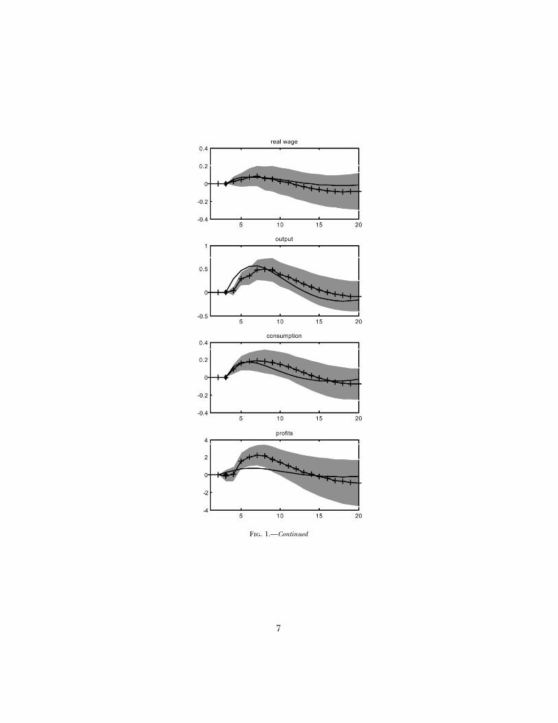
The impulse response functions of all variables in are displayed inYt

figure 1. Lines marked with a plus sign correspond to the point esti-mates. The shaded areas indicate 95 percent confidence intervals aboutthe point estimates.6 The solid lines pertain to the properties of ourstructural model, which will be discussed in Section III. The resultssuggest that after an expansionary monetary policy shock,

1. output, consumption, and investment respond in a hump-shapedfashion, peaking after about one and a half years and returning topreshock levels after about three years;

5 This sample period is the same as in Christiano et al. (1999).6 We use the method described in Sims and Zha (1999).

6

Fig. 1.—Model- and VAR-based impulse responses. Solid lines are benchmark modelimpulse responses; solid lines with plus signs are VAR-based impulse responses. Grey areasare 95 percent confidence intervals about VAR-based estimates. Units on the horizontalaxis are quarters. An asterisk indicates the period of policy shock. The vertical axis unitsare deviations from the unshocked path. Inflation, money growth, and the interest rateare given in annualized percentage points (APR); other variables are given in percentages.

7

Fig. 1.—Continued


TABLE 1Percentage Variance Due to Monetary Policy Shocks

4 QuartersAhead

8 QuartersAhead

20 QuartersAhead

Output 15(4,26)

38(15,48)

27(9,35)

Inflation 1(0,8)

4(1,11)

7(3,18)

Consumption 14(4,26)

21(5,37)

14(4,26)

Investment 10(2,21)

26(7,39)

23(6,32)

Real wage 2(0,8)

2(0,14)

4(0,15)

Productivity 15(3,25)

14(3,26)

10(3,20)

Federal funds rate 32(18,44)

19(8,27)

18(5,27)

M2 growth 19(8,29)

19(8,26)

19(8,24)

Real profits 13(5,25)

18(6,31)

7(2,20)

Note.—Numbers in parentheses are the boundaries of the associated 95 percent confidence interval.

2. inflation responds in a hump-shaped fashion, peaking after abouttwo years;

3. the interest rate falls for roughly one year;4. real profits, real wages, and labor productivity rise; and5. the growth rate of money rises immediately.

Interestingly, these results are consistent with the claims in Friedman(1968). For example, Friedman argued that an exogenous increase inthe money supply leads to a drop in the interest rate, which lasts oneto two years, and a rise in output and employment, which lasts two tofive years. Finally, the robustness of the qualitative features of our find-ings to alternative identifying assumptions and sample subperiods, aswell as the use of monthly data, is discussed in Christiano et al. (1999).

Our strategy for estimating the parameters of our model focuses ononly a component of the fluctuations in the data, namely the portionthat is caused by a monetary policy shock. It is natural to ask how largethat component is, since ultimately we are interested in a model thatcan account for all of the variation in the data. With this question inmind, table 1 reports variance decompositions. In particular, it displaysthe percentage of variance of the k-step-ahead forecast error in theelements of due to monetary policy shocks, for , 8, and 20.Y k p 4t

Numbers in parentheses are the boundaries of the associated 95 percent


confidence intervals.7 Notice that policy shocks account for only a smallfraction of inflation. At the same time, with the exception of real wages,monetary policy shocks account for a nontrivial fraction of the variationin the real variables. This last conclusion should be treated with caution.The confidence intervals about the point estimates are rather large.Also, while the impulse response functions are robust to the variousperturbations discussed in Christiano et al. (1999) and Altig et al.(2003), the variance decompositions can be sensitive. For example, theanalogous point estimates reported in Altig et al. are substantiallysmaller than those reported in table 1.

III. The Model Economy

In this section we describe our model economy and display the problemssolved by firms and households. In addition, we describe the behaviorof financial intermediaries and the monetary and fiscal authorities. Theonly source of uncertainty in the model is a shock to monetary policy.

A. Final-Good Firms

At time t, a final consumption good, , is produced by a perfectlyYt

competitive, representative firm. The firm produces the final good bycombining a continuum of intermediate goods, indexed by ,j � (0, 1)using the technology

1

1/lfY p Y dj , (3)( )t � jt0

where , and denotes the time t input of intermediate good1 ≤ l ! � Yf jt

j. The firm takes its output price, , and its input prices, , as givenP Pt jt

and beyond its control. Profit maximization implies the Euler equation

l /(l �1)f fP Yjtt p . (4)( )P Yjt t

Integrating (4) and imposing (3), we obtain the following relationshipbetween the price of the final good and the price of the intermediate

7 These confidence intervals are computed on the basis of bootstrap simulations of theestimated VAR. In each artificial data set we computed the variance decompositions cor-responding to the ones in table 1. The lower and upper bounds of the confidence intervalscorrespond to the 2.5 and 97.5 percentiles of simulated variance decompositions.


good:

1�lf1

1/(1�l )fP p P dj . (5)t � jt[ ]0

B. Intermediate-Goods Firms

Intermediate good is produced by a monopolist who uses thej � (0, 1)following technology:

a 1�a a 1�ak L � f if k L ≥ fjt jt jt jtY p (6)jt {0 otherwise,

where . Here, and denote the time t labor and capital0 ! a ! 1 L kjt jt

services used to produce the jth intermediate good. Also, denotesf 1 0the fixed cost of production. We rule out entry into and exit out of theproduction of intermediate good j.

Intermediate firms rent capital and labor in perfectly competitivefactor markets. Profits are distributed to households at the end of eachtime period. Let and denote the nominal rental rate on capitalkR Wt t

services and the wage rate, respectively. Workers must be paid in advanceof production. As a result, the jth firm must borrow its wage bill,

, from the financial intermediary at the beginning of the period.W Lt jt

Repayment occurs at the end of time period t at the gross interest rate,.R t

The firm’s real marginal cost is , wheres p �S(Y )/�Y S(Y ) pt t t

given by (6)}, where and .k k kmin {r k � w R l, Y r p R /P w p W /Pk,l t t t t t t t t t

Given our functional forms, we have

1�a a1 1 k a 1�as p (r ) (w R ) . (7)t t t t( ) ( )1 � a a

Apart from fixed costs, the firm’s time t profits are , where[(P /P) � s ]PYjt t t t jt

is firm j’s price.Pjt

We assume that firms set prices according to a variant of the mech-anism spelled out in Calvo (1983). This model has been widely used tocharacterize price-setting frictions. A useful feature of the model is thatit can be solved without explicitly tracking the distribution of pricesacross firms. In each period, a firm faces a constant probability, 1 �

, of being able to reoptimize its nominal price. The ability to reopti-yp

mize its price is independent across firms and time. If a firm can reop-timize its price, it does so before the realization of the time t growthrate of money. Firms that cannot reoptimize their price simply index


to lagged inflation:

P p p P . (8)jt t�1 j,t�1

Here, . We refer to this price-setting rule as lagged inflationp p P/Pt t t�1

indexation.Let denote the value of set by a firm that can reoptimize at timeP Pt jt

t. Our notation does not allow to depend on j. We do this in antic-Pt

ipation of the well-known result that, in models like ours, all firms thatcan reoptimize their price at time t choose the same price (see Woodford1996; Yun 1996). The firm chooses to maximizePt

�

l ˜E (by )v (P X � s P )Y , (9)�t�1 p t�l t tl t�l t�l j,t�llp0

subject to (4), (7), and

…p # p # # p for l ≥ 1t t�1 t�l�1X p (10)tl {1 for l p 0.

In (9), is the marginal value of a dollar to the household, which isvt

treated as exogenous by the firm. Later, we show that the value of adollar, in utility terms, is constant across households. Also, denotesEt�1

the expectations operator conditioned on lagged growth rates of money,, . This specification of the information set captures our as-m l ≥ 1t�l

sumption that the firm chooses before the realization of the time tPt

growth rate of money. To understand (9), note that influences firmPt

j’s profits only as long as it cannot reoptimize its price. The probabilitythat this happens for l periods is , in which case . Thel ˜(y ) P p P Xp j,t�l t tl

presence of in (9) has the effect of isolating future realizations ofl(y )p

idiosyncratic uncertainty in which continues to affect the firm’s profits.Pt

C. Households

There is a continuum of households, indexed by . The jthj � (0, 1)household makes a sequence of decisions during each period. First, itmakes a consumption decision and a capital accumulation decision, andit decides how many units of capital services to supply. Second, it pur-chases securities, whose payoffs are contingent on whether it can reop-timize its wage decision. Third, it sets its wage rate after finding outwhether it can reoptimize or not. Fourth, it receives a lump-sum transferfrom the monetary authority. Finally, it decides how much of its financialassets to hold in the form of deposits with a financial intermediary andhow much to hold in the form of cash.

Since the uncertainty faced by the household over whether it canreoptimize its wage is idiosyncratic in nature, households work different


amounts and earn different wage rates. So, in principle, they are alsoheterogeneous with respect to consumption and asset holdings. Astraightforward extension of arguments in Woodford (1996) and Erceg,Henderson, and Levin (2000) establishes that the existence of state-contingent securities ensures that, in equilibrium, households are ho-mogeneous with respect to consumption and asset holdings. Reflectingthis result, our notation assumes that households are homogeneous withrespect to consumption and asset holdings but heterogeneous with re-spect to the wage rate they earn and the hours they work.

The preferences of the jth household are given by

�

j l�tE b [u(c � bc ) � z(h ) � v(q )]. (11)�t�1 t�l t�l�1 j,t�l t�llp0

Here, is the expectation operator, conditional on aggregate andjEt�1

household j’s idiosyncratic information up to, and including, time t �; denotes time t consumption; denotes time t hours worked;1 c ht jt

denotes real cash balances; and denotes nominal cashq { Q /P Qt t t t

balances. When , (11) allows for habit formation in consumptionb 1 0preferences.

The household’s asset evolution equation is given by

aM p R [M � Q � (m � 1)M ] � A � Q � W ht�1 t t t t t j,t t j,t j,t

k ¯ ¯� R u k � D � P[i � c � a(u )k ]. (12)t t t t t t t t t

Here, is the household’s beginning of period t stock of money andMt

is time t labor income. In addition, , , and denote, respec-¯W h k D Aj,t j,t t t j,t

tively, the physical stock of capital, firm profits, and the net cash inflowfrom participating in state-contingent security markets at time t. Thevariable represents the gross growth rate of the economywide permt

capita stock of money, . The quantity is a lump-sum pay-a aM (m � 1)Mt t t

ment made to households by the monetary authority. The quantityis deposited by the household with a financialaM � Pq � (m � 1)Mt t t t t

intermediary, where it earns the gross nominal rate of interest, .R t

The remaining terms in (12), aside from , pertain to the stock ofPct t

installed capital, which we assume is owned by the household. Thehousehold’s stock of physical capital, , evolves according tokt

¯ ¯k p (1 � d)k � F(i , i ). (13)t�1 t t t�1

Here, d denotes the physical rate of depreciation, and denotes timeit

t purchases of investment goods. The function, F, summarizes the tech-nology that transforms current and past investment into installed capitalfor use in the following period. We discuss the properties of F below.

Capital services, , are related to the physical stock of capital bykt


. Here, denotes the utilization rate of capital, which we assume¯k p u k ut t t t

is set by the household.8 In (12), represents the household’s earn-k ¯R u kt t t

ings from supplying capital services. The increasing, convex functiondenotes the cost, in units of consumption goods, of setting the¯a(u )kt t

utilization rate to .ut

D. The Wage Decision

As in Erceg et al. (2000), we assume that the household is a monopolysupplier of a differentiated labor service, . It sells this service to ahjt

representative, competitive firm that transforms it into an aggregatelabor input, , using the following technology:Lt

1 lw

1/lwL p h dj .( )t � jt0

The demand curve for is given byhjt

l /(l �1)w wWth p L , 1 ≤ l ! �. (14)jt t w( )Wjt

Here, is the aggregate wage rate, that is, the price of . It is straight-W Lt t

forward to show that is related to via the relationshipW Wt jt

1�lw1

1/(1�l )wW p (W ) dj . (15)t � jt[ ]0

The household takes and as given.L Wt t

Households set their wage rate according to a variant of the mech-anism used to model price setting by firms. In each period, a householdfaces a constant probability, , of being able to reoptimize its nom-1 � yw

inal wage. The ability to reoptimize is independent across householdsand time. If a household cannot reoptimize its wage at time t, it sets

according toWjt

W p p W . (16)j,t t�1 j,t�1

8 Our assumption that households make the capital accumulation and utilization de-cisions is a matter of convenience. At the cost of more complicated notation, we couldwork with an alternative decentralization scheme in which firms make these decisions.


E. Monetary and Fiscal Policy

We assume that monetary policy is given by

…m p m � v e � v e � v e � . (17)t 0 t 1 t�1 2 t�2

Here, m denotes the mean growth rate of money, and is the responsevj

of to a time t monetary policy shock. We assume that the govern-E mt t�j

ment has access to lump-sum taxes and pursues a Ricardian fiscal policy.Under this type of policy, the details of tax policy have no impact oninflation and other aggregate economic variables. As a result, we neednot specify the details of fiscal policy.9

F. Loan Market Clearing, Final-Goods Clearing, and Equilibrium

Financial intermediaries receive from households and a trans-M � Qt t

fer, , from the monetary authority. Our notation here reflects(m � 1)Mt t

the equilibrium condition, . Financial intermediaries lend allaM p Mt t

their money to intermediate-goods firms, which use the funds to payfor . Loan market clearing requiresLt

W L p m M � Q . (18)t t t t t

The aggregate resource constraint is

c � i � a(u ) ≤ Y .t t t t

We adopt a standard sequence-of-markets equilibrium concept. In ourappendix, available on request, we discuss our computational strategyfor approximating that equilibrium. This strategy involves taking a linearapproximation about the nonstochastic steady state of the economy andusing the solution method discussed in Christiano (2002). For details,see the previous version of this paper (Christiano et al. 2001). In prin-ciple, the nonnegativity constraint on intermediate-goods output in (6)is a problem for this approximation. It turns out that the constraint isnot binding for the experiments that we consider, and so we ignore it.Finally, it is worth noting that since profits are stochastic, the fact thatthey are zero, on average, implies that they are often negative. As aconsequence, our assumption that firms cannot exit is binding. Allowingfor firm entry and exit dynamics would considerably complicate ouranalysis.

9 See Sims (1994) or Woodford (1994) for a further discussion.


G. Functional Form Assumptions

We assume that the functions characterizing utility are given by

u(7) p log (7),2z(7) p w (7) ,0

1�jq(7)v(7) p w . (19)q 1 � jq

In addition, investment adjustment costs are given by

itF(i , i ) p 1 � S i . (20)t t�1 t( )[ ]it�1

We restrict the function S to satisfy the following properties: S(1) p, and . It is easy to verify that the steady state of′ ′′S (1) p 0 k { S (1) 1 0

the model does not depend on the adjustment cost parameter, k. Ofcourse, the dynamics of the model are influenced by k. Given our so-lution procedure, no other features of the S function need to be spec-ified for our analysis.

We impose two restrictions on the capital utilization function, .a(u )tFirst, we require that in steady state. Second, we assumeu p 1t

. Under our assumptions, the steady state of the model is in-a(1) p 0dependent of . The dynamics do depend on . Given′′ ′j p a (1)/a (1) ja a

our solution procedure, we do not need to specify any other featuresof the function a.

IV. Econometric Methodology

In this section we discuss our methodology for estimating and evaluatingour model. We partition the model parameters into three groups. Thefirst group is composed of b, f, a, d, , , , and m. We setw w l b p0 q w

, which implies a steady-state annualized real interest rate of 3�0.251.03percent. We set , which corresponds to a steady-state share ofa p 0.36capital income roughly equal to 36 percent. We set , whichd p 0.025implies an annual rate of depreciation on capital equal to 10 percent.This value of d is roughly equal to the estimate reported in Christianoand Eichenbaum (1992a). The parameter f is set to guarantee thatprofits are zero in steady state. This value is consistent with the resultsof Hall (1988), Basu and Fernald (1994), and Rotemberg and Woodford(1999), who argue that economic profits are close to zero, on average.Although there are well-known problems with the measurement of prof-its, we think that zero profits is a reasonable benchmark.

The parameter was chosen to imply a steady-state value of L equalw0


to unity. Similarly, the parameter was set to ensure inw Q /M p 0.44q

steady state. This value is equal to the ratio of M1 to M2 at the beginningof our sample period. The rationale for using this ratio is that M1 is ameasure of money used for transactions, whereas M2 is a broader mon-etary aggregate. We reestimated the model calibrating to differentwq

steady-state values of . The primary impact on our parameter es-Q /Mtimates was to change the estimate of . The impulse response functionsjq

were relatively unaffected by different values of . The parameter m wasjq

set to 1.017, which equals the postwar quarterly average gross growthrate of M2. At our assumed parameter values, the steady-state velocityof money is given by

PY bp (m � q)(1 � a) p 0.36.

M m

This ratio is slightly below the average value, 0.44, of M2 velocity in oursample.

We set the parameter to 1.05. In numerical simulations we foundlw

that our results are robust to perturbations in this parameter.10 Ourspecification of implies a Frisch labor supply elasticity equal to unity.z(7)This elasticity is low by comparison with the values assumed in the realbusiness cycle literature.11 However, it is well within the range of pointestimates reported in the labor literature (see Rotemberg and Woodford1999).

We characterize monetary policy by (17), where the ’s are the im-vi

pulse responses implied by our estimated VAR:

4 �1…m p t(I � A L � � A L ) ce .t 1 4 t

Here, c is the last column of C, and , C are the estimatedA , … , A1 4

parameters of our VAR. In addition, t is a row vector with zeros every-where, except unity in the last element. The moving average parameter,

, is the coefficient on in the expansion of the polynomial to theiv Li

right of the equality in the previous expression, for . Toi p 0, 1, …incorporate this representation of monetary policy into the model, weuse the procedure described by King and Watson (1996). Christiano etal. (1998) show that this representation is not statistically significantlydifferent from the one generated by a first-order autoregression with acoefficient roughly equal to 0.5.

The third group of model parameters is .g { (l , y , y , j , k, b, j )f w p q a

10 Holding fixed the other parameter values at their benchmark values reported below,we found that the impulse response functions implied by the model are insensitive todifferent values of .lw

11 For example, the Frisch elasticity implicit in the “divisible labor” model in Christianoand Eichenbaum (1992a) is roughly 2.5 percent.


TABLE 2Estimated Parameter Values

Model lf yw yp jq k b ja n

Benchmark 1.20(.06)

.64(.03)

.60(.08)

10.62(.67)

2.48(.43)

.65(.04)

.01 NA

Flexible prices 1.11(.05)

.65(.02)

0 8.63(.63)

3.24(.47)

.66(.04)

.01 NA

Unconditionalindexation

1.36(.09)

.49(.07)

.72(.16)

11.09(.67)

1.92(.35)

.63(.05)

.01 NA

No variable capitalutilization

1.85(.13)

.42(.05)

.92(.02)

10.83(.67)

1.58(.28)

.62(.05)

100 NA

No habit formation 1.01(.04)

.80(.02)

.28(.15)

10.12(.70)

.91(.18)

0 .01 NA

Small adjustmentcosts ininvestment

1.06(.04)

.76(.03)

.64(.08)

10.92(.70)

.5 .52(.11)

.01 NA

Lucas-Prescott in-vestment adjust-ment costs

1.08(.06)

.62(.03)

.53(.23)

10.60(.60)

NA .71(.03)

.01 �.74(.22)

No working capital 1.25(.06)

.46(.05)

.89(.02)

10.85(.67)

1.89(.37)

.62(.05)

.01 NA

Note.—Standard errors are in parentheses.

These parameters were estimated by minimizing a measure of the dis-tance between the model and empirical impulse response functions.Let denote the mapping from g to the model impulse responseW(g)functions, and let denote the corresponding empirical estimates. WeW

include the first 25 elements of each response function, excluding thosethat are zero by assumption. Our estimator of g is the solution to

′ �1ˆ ˆJ p min [W � W(g)] V [W � W(g)]. (21)g

Here, V is a diagonal matrix with the sample variances of the ’s alongW

the diagonal. These variances are the basis for the confidence intervalsreported in figure 1. So, with this choice of V, g is effectively chosenso that lies as much as possible inside these confidence intervals.W(g)

V. Empirical Results

In this section we discuss the estimated parameter values. In addition,we assess the ability of the estimated model to account for the impulseresponse functions discussed in Section II.

A. Parameter Estimates

The row labeled “benchmark” in table 2 summarizes our point estimatesof the parameters in the vector g. With the exception of , standardja


errors are reported in parentheses.12 We do not report a standard errorfor because our estimation procedure drives that parameter towardja

zero, at which point the algorithm breaks down. As a result, we simplyset and optimize the estimation criterion over the remainingj p 0.01a

elements in g. To interpret this low value of , consider the Eulerja

equation associated with the household’s capital utilization decision:

k ′E w[r � a (u )] p 0. (22)t�1 t t t

According to this expression, the expected marginal benefit of raisingutilization must equal the associated expected marginal cost. After lin-earizing this expression about the nonstochastic steady state, we obtain13

1 kˆ Ê r � u p 0. (23)t�1 t t[ ]ja

From this expression we can see that is the elasticity of capital1/ja

utilization with respect to the rental rate of capital. So a small value ofcorresponds to a large elasticity. Below, we provide evidence on theja

empirical plausibility of our model’s implications for capacity utilization.We now discuss the remaining parameters in table 2. Our point es-

timate of implies that wage contracts last, on average, 2.8 quarters.yw

Our point estimate of implies that price contracts last, on average,yp

2.5 quarters. While the standard errors on and are small, later wey yp w

shall see that, in fact, sticky wages play a more important role in themodel fit than sticky prices.

To interpret the point estimate of , it is useful to note that thejq

household’s first-order condition for cash balances, , isQ t

′v (q ) � w p wR , (24)t t t t

where . Here, is the marginal utility of units of currency.q p Q /P w Pt t t t t

That is, , where is the Lagrange multiplier on the household’sw p v P vt t t t

budget constraint, (12). According to (24), the marginal utility of adollar allocated to cash balances must equal the marginal utility of adollar allocated to the financial intermediary. To interpret , note thatwt

the household’s optimization problem implies

E u p E w. (25)t�1 c,t t�1 t

Here, is the realized value of the marginal utility of consumption atuc,t

12 Standard errors were computed using the asymptotic delta function method appliedto the first-order condition associated with (21).

13 Here, we have used the fact that we impose , where denotes the rental ratek ′ kr p a ron capital in steady state. This rental rate is determined solely by b and d.


date t:

�u(c � bc ) �u(c � bc )t t�1 t�1 tu p � bE . (26)c,t t�c �ct t

According to (25) and (26), in the absence of uncertainty, would bewt

the marginal utility of consumption. So (24) relates real cash balancesto the nominal interest rate as well as to consumption flows.

Log-linearizing (24) and imposing (19), we obtain

1 R ˆˆq p � R � w . (27)t t t( )j R � 1q

Here and throughout the paper, a hat over a variable denotes thepercentage deviation from its steady-state value. Equation (27) impliesthat, with held constant, the interest semielasticity of money demandwt

is

� log q 1t� p .�R 4j (R � 1)t q

This expression takes into account that the time period of the modelis quarterly and the elasticity is measured with respect to the annualizedrate of interest. Our parameter estimates imply that this elasticity is 0.96;that is, a one-percentage-point rise in the annualized rate of interestleads to a 0.96 percent reduction in real balances. This elasticity isconsiderably smaller than standard estimates reported for static moneydemand equations. For example, the analogous number in Lucas (1988)is 8.0. We found that our estimate of is driven primarily by the model’sjq

attempt to replicate the initial responses of the interest rate to a mon-etary policy shock. Consequently, we interpret our interest semielasticityas pertaining to the short-run response of money demand. This semi-elasticity is often estimated to be quite small (see Christiano et al. 1999).

To interpret the point estimate of k, it is useful to consider the house-hold’s first-order condition for investment:

E w p E [wP F � bw P F ]. (28)′ ′t�1 t t�1 t k ,t 1,t t�1 k ,t�1 2,t�1

Here, is the partial derivative of the investment adjustment cost func-Fj,t

tion, , defined in (20), with respect to its jth argument, ,F(i , i ) j p 1t t�1

2. Also, is the shadow value, in consumption units, of a unit ofP ′k ,t

as of the time that the household makes its period t investment andkt�1

capital utilization decision. The variable is what the price of installedP ′k ,t

capital would be if there were a market for at the beginning ofkt�1

period t.The left side of (28) is the marginal cost, in utility terms, of a unit

of investment goods. The right side of (28) is the associated marginal


benefit. To understand the benefit, note that an extra unit of investmentgoods produces extra units of . The value of these goods, in utility¯F k1,t t�1

terms, is . An increase in also affects the quantity of installedP F E w i′k ,t 1,t t�1 t t

capital produced in the next period by . The last term in (28)F2,t�1

measures the utility value of these additional capital goods.Log-linearizing (28) about the steady state, we obtain

ˆ ˆ ˆ ˆ ˆP p kE [ı � ı � b(ı � ı )],′k ,t t�1 t t�1 t�1 t

so that

�1 j ˆˆ ˆı p ı � b E P .′�t t�1 t�1 k ,t�jk jp0

According to this expression, is the elasticity of investment with1/k

respect to a 1 percent temporary increase in the current price of in-stalled capital. Our point estimate implies that this elasticity is equal to0.40. A more persistent change in the price of capital induces a largerpercentage change in investment because adjustment costs induceagents to be forward looking. For example, a permanent 1 percentchange in the price of capital induces a percent1/[k(1 � b)] p 55change in investment.

The literature on Tobin’s q also reports empirical estimates of in-vestment elasticities. It is difficult to compare these estimates with oursbecause the Tobin’s q literature is based on a first-order specificationof adjustment costs, that is, one in which adjustment costs depend onlyon the current level of investment (i.e., the first derivative of the capitalstock). Given this specification, only the current value of enters intoP ′k ,t

. In contrast, we assume a second-order specification of adjustmentıt

costs, that is, one in which the costs depend on the second derivativeof the capital stock. From our perspective, the elasticities reported inthe Tobin’s q literature represent a combination of k and the degree ofpersistence in . Later, we document why it is important to allow forP ′k ,t

second-order rather than first-order adjustment costs in our analysis.Our point estimate of the habit parameter b is 0.65. This value is close

to the point estimate of 0.7 reported in Boldrin, Christiano, and Fisher(2001). Those authors argue that the ability of standard general equi-librium models to account for the equity premium and other asset mar-ket statistics is considerably enhanced by the presence of habit formationin preferences. Below we discuss the role that habit formation plays inthe fit of our model. Finally, the estimated value of , 1.20, is close tol f

the values used in the literature (see, e.g., Rotemberg and Woodford1995).


B. Properties of the Estimated Model

The impulse response functions of the model to a one-standard-devia-tion monetary policy shock are represented by the solid lines in figure1. A number of results are worth emphasizing here. First, the modeldoes well at accounting for the dynamic response of the U.S. economyto a monetary policy shock. Most of the model responses lie within thetwo-standard-deviation confidence interval computed from the data.Second, the model succeeds in accounting for the inertial response ofinflation. Indeed, there is no noticeable rise in inflation until roughlythree years after the policy shock. This result is particularly notable,since firms and households in our model change prices and wages, onaverage, only once every 2.5 quarters.

Third, the model generates a very persistent response in output. Thepeak effect occurs roughly one year after the shock. The output responseis positive for nine quarters, during which the cumulative output re-sponse is 3.14 percent. Over 78 percent of this cumulative rise occursafter the typical wage and price contract in effect at the time of theshock has been reoptimized. The part of the output response that occursbeyond the length of the typical contract reflects, to a first approxi-mation, the staggering of wages and prices. A different way to quantifythe effect of staggering is to consider a statistic that is analogous to theone proposed by Chari et al. (2000). This statistic is constructed asfollows. First, calculate the amount of time it takes the output expansioncaused by a positive policy shock to go to zero. Then, calculate the ratioof this number to the number of periods in a typical contract. FollowingChari et al., we call this ratio the contract multiplier. In our benchmarkmodel, this statistic is 3.7.14 So, both of our statistics indicate that stag-gering of contracts contributes substantially to the propagation of mon-etary policy shocks. As we show below, this property depends criticallyon the real frictions embedded in our benchmark model.

Figure 2 provides a different way of illustrating the persistent outputresponse and the inertial inflation response to a monetary policy shock.There, we display the response of the price level, the money stock, andoutput in the model. Each is expressed as a percentage of its level alongthe unshocked growth path. Notice how the money stock rises to itspeak level by the third quarter after the shock and is roughly back towhere it started by the middle of the third year. Despite the prolongedrise in the money stock, there is essentially no change in the price level.

14 Our measure of the contract multiplier differs from the one in Chari et al. (2000).Theirs is based on a measure of the half-life of a shock, namely the number of periodsit takes for the response of a variable to fall to one-half of its response in the initial periodof the shock. We cannot apply this half-life measure to output because the initial responseof output to a policy shock is zero.


Fig. 2.—Response of price level, output, and money stock to an expansionary monetarypolicy shock in the benchmark model.

At the same time, there is a prolonged boom in output that lasts evenafter the boom in the money supply is over. The peak in output is almosttwice as big as the peak in the money supply, with the former occurringone-half of a year after the latter.

Returning to figure 1, notice that the model is able to account forthe dynamic response of the interest rate to a monetary policy shock.


Consistent with the data, an expansionary monetary policy shock in-duces a sharp decline in the interest rate, which then returns to itspreshock level within a year. It is interesting that a policy shock inducesa more persistent effect on output than on the interest rate. Indeed,the peak effect on output occurs one quarter after the policy variablehas returned to its steady-state value. So, regardless of whether we mea-sure policy by the money stock or the interest rate, the effects of a policyshock on aggregate variables persist beyond the effects on the policyvariable itself. This property reflects the strong internal propagationmechanisms in the model.

Next note that, as in the data, the real wage rises by a small positiveamount in response to the policy shock. In addition, consumption andinvestment exhibit persistent, hump-shaped rises that are consistent withour VAR-based estimates. Figure 1 also shows that both productivity andprofits rise in response to a monetary policy shock. While the extent ofthe rise is not as large as our VAR-based estimates, it is interesting thatthere is any rise at all. We discuss this further below.

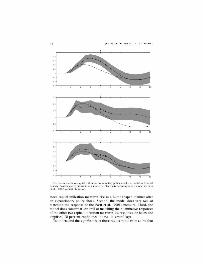
We conclude by assessing the model’s implications for capital utili-zation. In practice, there are several competing measures of capitalutilization, each of which is imperfect in a different way.15 We consideredthree alternatives and compared their response to a policy shock withthe implications of our model. The first is the Federal Reserve Board’stime series on capacity utilization, which measures the intensity withwhich all factors of production are used in the industrial productionsector (see Christiano 1984; Shapiro 1989). The second is the FederalReserve Board’s time series on electricity consumption in the industrialproduction sector. This is a useful measure of capital utilization underthe assumption that capital services and electricity are used in fixedproportions (see Burnside, Eichenbaum, and Rebelo 1995). The thirdmeasure of capital utilization, developed in Basu, Fernald, and Shapiro(2001), pertains to the economy as a whole. This measure is based onthe assumption that capital services are tied to the workweek of capital,as measured by average hours worked.

Figure 3 displays the dynamic response of capital utilization in ourestimated model, along with the corresponding empirical estimates,based on our three measures of capital utilization. These estimates wereobtained by constructing three different VARs. Each augments ourbenchmark VAR with one of the alternative measures of capital utili-zation. Consistent with our model, we assume that capital utilizationdoes not respond contemporaneously to a monetary policy shock. Anumber of results are worth noting. First, consistent with the model, all

15 For surveys of different approaches to measuring capacity utilization, see Christiano(1984) and Shapiro (1989).


Fig. 3.—Response of capital utilization to monetary policy shocks: a, model vs. FederalReserve Board capacity utilization; b, model vs. electricity consumption; c, model vs. Basuet al. (2000) capital utilization.

three capital utilization measures rise in a hump-shaped manner afteran expansionary policy shock. Second, the model does very well atmatching the response of the Basu et al. (2001) measure. Third, themodel does somewhat less well at matching the quantitative responsesof the other two capital utilization measures. Its responses lie below theempirical 95 percent confidence interval at several lags.

To understand the significance of these results, recall from above that


our estimation procedure drives to its lower bound in an attempt toja

increase the elasticity of the supply of capital services. As we explainbelow, the resulting strong response of capital utilization to a monetarypolicy shock plays a significant role in the model’s performance. So itis important to determine whether the model relies too heavily on acounterfactually strong response of utilization. The results in figure 3indicate that, if anything, the model understates the response ofutilization.

VI. Understanding the Key Features of the Model

This section is organized into two parts. First, we provide intuition forhow the different features of our model contribute to our results. Sec-ond, we illustrate this intuition through a series of quantitative exercises.

A. Qualitative Considerations

To describe the intuition for the monetary transmission mechanism inour model, it is useful to proceed in two steps. First, we provide intuitionfor why consumption, investment, output, employment, productivity,profits, and capital utilization rise whereas the interest rate falls. Thisdiscussion takes as given the inertial behavior of prices and wages. Inour second step, we provide intuition for why prices and wages respondslowly to a monetary policy shock. Of course, in general equilibrium,all effects occur simultaneously. Still, to highlight the different frictionsin our model, we find it useful to proceed in this sequential manner.

To understand the contemporaneous effect of a policy shock, it isuseful to focus on the money market–clearing condition, (18), and thehousehold’s first-order condition, (24), for cash balances, . Given ourQ t

assumptions, the full amount of a policy shock–induced money injectionmust be absorbed by household cash holdings, . Firms do not wishQ t

to absorb any part of a cash infusion because does not respond toW Lt t

a policy shock. The wage rate, , is predetermined because the ’sW Wt jt

are predetermined by assumption. Employment, , is predeterminedLt

because we assume that consumption, investment, and capital utilizationare predetermined. It follows from (18) that a period t money injectionmust be accompanied by an equal increase in .Q t

To understand the impact of the rise in on , suppose for theQ Rt t

moment that is constant. Since is predetermined, the rise inw P Qt t t

corresponds to a rise in real balances. According to (24), must fallR t

to induce households to increase real cash balances, . In practice,Q /Pt t

we found that falls, but by only a relatively small amount. Finally, sincewt

falls and the firm’s wage bill and revenues are unaffected by theR t

shock, profits must rise.


We now turn to the dynamic effects of a monetary shock on , ,R Ct t

, , , , productivity, and profits. The persistent drop in reflectsI Y L u Rt t t t t

the slow adjustment of relative to its high value in the period ofQ /Pt t

the shock. In part, this sluggish adjustment is due to the inertia in .Pt

But it is also the case that households are slow to reduce their cashholdings from their high level in the impact period of the shock. Thisslow response in reflects money market clearing, (18), the inertialQ t

behavior of , and the slow rise of after a policy shock. The slowW Lt t

expansion in hours worked occurs because household demand for goodsrises slowly, in a hump-shaped manner, reflecting habit formation inpreferences and second-order adjustment costs in investment. Theseconsiderations provide intuition for the persistent rise in after anQ /Pt t

expansionary monetary policy shock. It then follows from (24) that R t

must be low for a prolonged period of time.16 The hump-shaped re-sponse in and implies that output, employment, and capital utili-C It t

zation rates also rise in a hump-shaped manner. Finally, the rise inproductivity reflects the effects of capital utilization, as well as the pres-ence of the fixed cost in the production function.

Note that our mechanism for generating a persistent liquidity effectcontrasts with the approach in the recent literature, which emphasizesfrictions in the adjustment of financial portfolios (see, e.g., Christianoand Eichenbaum 1992b; Alvarez, Atkeson, and Kehoe 2002). These typesof frictions are absent from our model, where the liquidity effect is anindirect consequence of nonfinancial market frictions.

The previous intuition takes as given the inertial responses of pricesand wages to a monetary policy shock. We now discuss the features ofour model that allow it to generate inertial price and wage behavior.

To understand price inertia, recall that the firm chooses to maxi-Pt

mize (9) subject to (4), (7), and (10). The log-linearized first-ordercondition associated with this problem is

� �

l lˆ ˆ ˆ ˆ ˆ ˆp p E s � (by )(s � s ) � (by )(p � p ) . (29)� �t t�1 t p t�l t�l�1 p t�l t�l�1[ ]lp1 lp1

Here, , and recall that a hat over a variable indicates the per-˜p p P /Pt t t

centage deviation from its steady-state value. That is, . Aˆ ˜ ˜ ˜p p (p � p)/pt t

variable without a hat or a subscript indicates its nonstochastic steady-state value. Several features of (29) are worth noting. First, if inflationand real marginal cost are expected to remain at their time t levels,then the firm sets . Second, suppose that the firm expects realˆ ˆp p E st t�1 t

marginal costs to be higher in the future than at time t. Anticipating

16 As in the impact period, the movements in are sufficiently small that they can bewt

ignored for purposes of intuition.


those future marginal costs, the firm sets higher than . It doesˆ ˆp E st t�1 t

so because it understands that it may not be able to raise its price whenthose higher marginal costs materialize. We refer to this type of forward-looking behavior as “front-loading.” Third, suppose that firms expectinflation in the future to rise above . The one-period lag in theÊ pt�1 t

dynamic price-setting rule, (8), implies that the firm’s relative pricewould fall.

It follows from well-known results in the literature that (5) can beexpressed as

1/(1�l ) 1/(1�l ) 1�l˜ f f fP p [(1 � y )(P ) � y (p P ) ] . (30)t p t p t�1 t�1

Dividing by , linearizing, and rearranging, we obtainPt

ypˆ ˆ ˆp p (p � p ). (31)t t t�11 � yp

Relations (29) and (31) imply

1 b (1 � by )(1 � y )p p ˆˆ ˆ ˆp p p � E p � E s . (32)t t�1 t�1 t�1 t�1 t1 � b 1 � b (1 � b)yp

When we impose , (32) is equivalent toj ˆ Ê b (p � p ) r 0t�1 t�j t�j�1

�(1 � by )(1 � y )p p jˆˆ ˆp � p p E b s . (33)�t t�1 t�1 t�jy jp0p

Four features of (33) are worth noting. First, consistent with ourtiming assumptions, (33) implies that does not respond to a periodpt

t monetary policy shock. Second, inflation depends on expected futuremarginal costs. So, other things equal, the more inertial marginal costsare, the more inertial inflation is. Relation (7) implies that marginalcost is an increasing function of the wage rate, the rental rate on capital,and the interest rate. From this perspective, a key function of nominalwage rigidities is to induce inertia in inflation. Variable capital utiliza-tion, by increasing the elasticity of the supply of capital services, dampensthe rise in the rental rate of capital. For this effect to be operative, ut

must rise in the wake of an expansionary policy shock. Our assumptionthat the cost of increased capital utilization is given in terms of outputplays a role in ensuring that this rise occurs. If, for example, the costwere a higher capital depreciation rate, then could actually fall. Tout

see this, note that after an expansionary policy shock, investment in-creases. In the presence of investment adjustment costs, this implies thatthe marginal cost of physical capital rises. This increase in turn leadsto a rise in the cost of , which could lead to a fall in the utilizationut

of capital.


The third feature of relation (33) worth noting follows from the factthat the interest rate appears in firms’ marginal cost. Since the interestrate drops after an expansionary monetary policy shock, the modelembeds a force that pushes marginal costs down for a period of time.Indeed, in the estimated benchmark model the effect is strong enoughto induce a transient fall in inflation.

Fourth, according to (33), current inflation depends on lagged in-flation. This induces an extra source of inertia in the rate of inflation,which is not present in the standard formulation of Calvo-style pricingfrictions. For example, Yun (1996) and others assume that firms thatdo not reoptimize their price reset it according to . Here, pP p pPjt jt�1

is the steady-state inflation rate. With this static indexation formulation,(32) is replaced by

(1 � by )(1 � y )p p ˆˆ ˆp p bE p � E s , (34)t t�1 t�1 t�1 typ

and (33) holds without the lagged inflation term. Authors like Fuhrerand Moore (1995) and Gali and Gertler (1999) argue on empiricalgrounds that lagged inflation belongs in an expression like (34). Ourlagged inflation indexation pricing rule provides one way to rationalizethe presence of such an inflation term.

B. Quantitative Considerations

We now analyze how the various features of the model contribute quan-titatively to its performance. We do this by considering two sets of modelperturbations. The first pertains to the nominal part of the model andfocuses on the role of price and wage frictions, as well as the represen-tation of monetary policy. The second focuses on the role of severalfeatures of the real economy.

1. Nominal Side of the Model Economy

It is commonplace in the literature to represent monetary policy as aparsimonious Taylor rule. To assess the model’s properties when werepresent policy this way, we replace the money growth rule, (17), withthe following Taylor rule:

ˆ ˆ ˆˆR p rR � (1 � r)(a E p � a y ) � e .t t�1 p t�1 t�1 y t t

Here, is a shock to monetary policy. In addition, we chose values foret

the parameters consistent with the post-1979 era estimates reported byClarida, Gali, and Gertler (1999): , , and . Rowr p 0.80 a p 1.5 a p 0.1p y

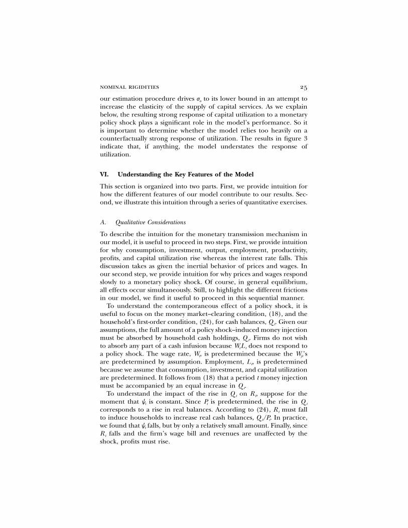
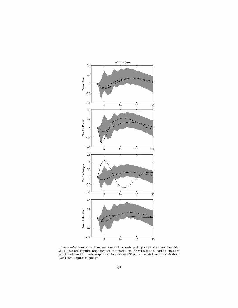
1 of figure 4 displays the dynamic response of inflation and output in


this version of the model, along with the benchmark responses. Noticethat the response functions are similar in the two versions of the model.The main difference is that the overall rise in output is smaller in theTaylor rule version. Still, inflation exhibits substantial inertia, and outputexhibits substantial persistence.

Next, we consider the role of sticky prices in the performance of thebenchmark model. Row 2 in figure 4 displays the impulse responsefunctions for a version of the model in which we set and holdy p 0p

the remaining parameters at their benchmark values. Notice that theresponse of inflation and output is not substantially affected by thischange. The main impact is that inflation falls more and there is a largerrise in output in the immediate aftermath of a shock relative to thebenchmark model. The fall in inflation reflects the impact of the fallin the interest rate on marginal cost. Somewhat paradoxically, stickyprices play the role of muting the fall in prices that would otherwiseoccur after an expansionary monetary policy shock. In any event, evenwithout sticky prices, inflation continues to display substantial inertia,and output continues to rise in a hump-shaped manner.

A different way to assess the impact of sticky prices is to reestimateour model, subject to the constraint . The resulting point esti-y p 0p

mates are reported in table 2. Interestingly, inference about model pa-rameters is quite robust to imposing the restriction . Notice iny p 0p

particular that our point estimate of is virtually unaffected. The im-yw

pulse response functions for inflation and output are very similar towhat is displayed in row 2 of figure 4. So, with , the model stilly p 0p

generates large, persistent increases in output and an inertial responsein inflation. These observations substantiate our claim that sticky pricesplay a limited role in accounting for the good fit of the benchmarkmodel.

We now turn to sticky wages, which turn out to play a crucial role inthe model’s performance. Row 3 in figure 4 displays the impulse re-sponse functions for a version of the model in which we set andy p 0w

hold the remaining parameters at their benchmark values. Now inflationsurges in the aftermath of a policy shock. This surge reflects a sharp,persistent rise in real wages (not displayed). Notice also that outputrises only a small amount in the first period after the shock and thenquickly returns to its preshock growth path. When we attempted toestimate the model with , the estimate of was driven to unity.y p 0 yw p

Evidently, the estimation criterion prefers extreme degrees of price stick-iness when there are no sticky wages. Clearly, sticky wages play a crucialrole in allowing the model to account for the effects of a monetarypolicy shock.

Next, we turn to the role of lagged versus static inflation indexation.Row 4 in figure 4 displays the impulse response functions for a version

30

Fig. 4.—Variants of the benchmark model: perturbing the policy and the nominal side.Solid lines are impulse responses for the model on the vertical axis; dashed lines arebenchmark model impulse responses. Grey areas are 95 percent confidence intervals aboutVAR-based impulse responses.

31

Fig. 4.—Continued


of the model in which prices are set according to the static inflationindexation scheme. Notice that the model properties are not substan-tially affected by this change. Inflation continues to be inertial, andthere is still a persistent rise in output after a monetary policy shock.Another way to assess the impact of the price-setting scheme is to rees-timate the model under static inflation indexation. The parameter es-timates are reported in table 2. Two things are worth noting. First,consistent with the discussion in subsection A, the degree of price stick-iness required to match the empirical impulse response functions isgreater under the static price-updating scheme. For example, the av-erage duration of price contracts rises from 2.5 quarters to almost ayear. In contrast, the average duration of wage contracts declines fromroughly 2.8 quarters to about two quarters. Of course, once samplinguncertainty is taken into account, the differences between the two mod-els are less dramatic. Second, the estimated degree of market powerrises from 1.20 to 1.36 in the static price-updating version of the model.Again, if sampling uncertainty is taken into account, the differences arenot significant. So, while there are marginal improvements with ourlagged inflation indexation scheme, they are not critical to the model’sperformance.

2. The Role of Timing Assumptions in the Model

Our benchmark model incorporates various timing assumptions thatensure it is consistent with the assumptions used to identify a monetarypolicy shock in our VAR. These assumptions do not have a substantialimpact on the dynamic properties of the model. Here, we illustrate thisclaim by examining the impact of timing on the output and inflationresponse to a policy shock. The solid line in row 1 of figure 5 displaysthe response of inflation and output when we drop the assumption thatconsumption, investment, and capital utilization are predetermined. Forconvenience, the dashed line reproduces the responses in the bench-mark model. While output now rises in the impact period of the shock,the magnitude and persistence of the response, as well as its hump-shaped pattern, are similar across the two models. Notice also that theproperties of inflation are virtually unaffected.

The solid line in row 2 of figure 5 displays the response of inflationand output when we drop the assumption that wages and prices are setbefore the policy shock is realized. With this change, inflation drops bya small amount in the impact period of a shock, reflecting the drop inthe interest rate. Still, the dynamic response of inflation in the twomodels is very similar. Moreover, the response of output is virtuallyidentical in the two models.


Fig. 5.—Role of timing in model dynamics. Solid lines are impulse responses for themodel on the vertical axis; dashed lines are benchmark model impulse responses. Greyareas are 95 percent confidence intervals about VAR-based impulse responses.

3. Real Side of the Model Economy

In this subsection, we evaluate the role of the different real frictionsembedded in our benchmark model. Our primary conclusions are asfollows. The key real friction that allows the model to generate an inertialinflation response and a persistent output response to a policy shock isvariable capital utilization. The primary role of the other frictions—investment adjustment costs, habit formation in consumption, and work-ing capital—is to enable the benchmark model to account for the re-sponse of other variables to a policy shock.

Row 1 in figure 6 reports the effects of a monetary policy shock oninflation and output when we do not allow for variable capital utilization

. The remaining model parameters are fixed at their bench-(j p 100)a

mark values. Notice that the output effect of a monetary shock is roughlycut in half when variable capitalization is dropped from the model. Also,inflation rises substantially more in the immediate aftermath of a mon-etary policy shock. A different way to assess the importance of variablecapital utilization is to consider the results in table 2. There we reportthe results of reestimating the parameters of the benchmark model,fixing . Note that our point estimate of is now 0.92, implyingj p 1,000 ya p

an average duration of price contracts equal to a little over three years.This is clearly inconsistent with existing microeconomic evidence (see,e.g., Bils and Klenow 2004). In addition, our point estimate for jumpsl f

to 1.85, implying a markup well above standard estimates. We conclude

34

Fig. 6.—Variants of the benchmark model: perturbing the real side of the model econ-omy. Solid lines are impulse responses for the model on the vertical axis; dashed linesare benchmark model impulse responses. Grey areas are 95 percent confidence intervalsabout VAR-based impulse responses.

35

Fig. 6.—Continued


that variable capital utilization plays a critical role in the model’s per-formance.

Row 2 in figure 6 reports the effects of a monetary policy shock oninflation and output when we eliminate habit formation (i.e., )b p 0and hold all other parameters at their benchmark values. Now, a policyshock leads to a larger initial rise in output and a slightly larger rise ininflation than in the benchmark model. The increase in output reflectsthe way that consumption responds to the policy shock. In results notdisplayed here, we found that the maximal impact on consumptionoccurs in the period immediately after the shock. After that, consump-tion slowly declines back to its preshock level. This temporal patterncan be understood as follows. When , households relate the growthb p 0rate of consumption to the level of the interest rate, which is low aftera shock. Intertemporal budget balance requires that this downward-sloped consumption profile start from an initially high level of con-sumption.

An implication of the previous argument is that, with , there isb p 0no way to reconcile a hump-shaped response of consumption with alow interest rate. With habit formation , it is possible to reconcile(b 1 0)the two. Roughly speaking, with habit formation, households relate thechange in the growth rate of consumption to the interest rate. So, witha low interest rate, households choose a consumption profile charac-terized by a declining growth rate of consumption. Intertemporal bud-get balance implies that this profile begins with a positive growth rate.This explains why the benchmark model with generates a hump-b 1 0shaped consumption profile in conjunction with a low interest rate.

Table 2 reports the results of reestimating the parameters of thebenchmark model, subject to . Notice that inference about pa-b p 0rameters is sensitive to this change in the real side of the model economy.For example, our estimate of the parameter k drops from 2.48 in thebenchmark model to 0.91 in the model with . In an experimentb p 0not reported here, we found that the drop in k encourages a strongerinvestment response and a weaker consumption response. The lattereffect moves the no habit formation model into closer conformity withthe data.

Row 3 in figure 6 reports the effects of a monetary policy shock oninflation and output when investment adjustment costs are very small(i.e., ) and we hold all other parameters at their benchmarkk p 0.5values.17 Now, a policy shock leads to a substantially larger initial rise inoutput and inflation relative to the benchmark model. This patternreflects the fact that investment surges more than in the benchmark

17 We encountered difficulties with our solution algorithm when we tried to solve themodel setting k equal to zero. This is why we do not report results for the case .k p 0


model. To understand why, it is useful to consider the rate of returnon capital. Holding capital utilization constant, we have

kr � P (1 � d)′t�1 k ,t�1 ,P ′k ,t

where is defined after equation (28). Our model implies that anP ′k ,t

expansionary monetary policy shock leads to a persistent fall in the realinterest rate, . When one abstracts from risk considerations, equi-R /pt t�1

librium requires that the rate of return on capital fall with the realinterest rate. Suppose that there are no adjustment costs, so that

. In this case, the rate of return formula reduces toP p P p 1′ ′k ,t k ,t�1

. When we hold the markup constant, the only way the ratekr � 1 � dt�1

of return on capital can fall is if its rental rate and marginal productfall. This fall in turn requires a surge in investment. This rise in in-vestment is what accounts for the strong rise in output observed in row3 of figure 6. When there are adjustment costs in investment, it is pos-sible for the rate of return on capital to fall without any counterfactuallylarge rise in investment, as long as there is an appropriate intertemporalpattern in . Table 2 reports the results of reestimating the parametersP ′k ,t

of the benchmark model subject to . Interestingly, here there isk p 0.5very little sensitivity in parameters.

We now consider the impact of the way we modeled adjustment costsin investment. Recall that in the benchmark model, firms face second-order costs of changing investment. It is more typical in the businesscycle literature to work with the first-order adjustment costs. For earlyreferences, see Eisner and Strotz (1963), Lucas (1967a, 1967b), andLucas and Prescott (1971). For more recent examples, see McCallumand Nelson (1999) and Chari et al. (2000). To assess the performanceof the model with first-order adjustment costs, we replace (13) with theadjustment cost formulation in Christiano and Fisher (1998):

¯ ¯k ≤ Q((1 � d)k , i ).t�1 t t

Here

n n 1/nQ(x, z) p (a x � a z ) ,1 2

and . In this expression, x denotes previously installed capital aftern ≤ 1depreciation and z denotes new investment goods. The scalars ,a 1

were chosen to guarantee that in the nonstochastica 1 0 Q p Q p 12 x z

steady state.18 When , the above technology corresponds to then p 1conventional linear capital accumulation equation. The case of adjust-

18 In steady state, , and . It is straightforward to confirm that, with¯ ¯x p (1 � d)k z p dkand , in steady state.1�w 1�wa p (1 � d) a p d Q p Q p 11 2 x z


ment costs corresponds to . Here, the marginal product of newn ! 1investment goods is decreasing in the flow of investment.

We reestimated all the parameters of this model, including n. We referto this model as the alternative adjustment cost model. Our results arereported in table 2. Two results are of interest. First, apart from n, theestimated parameters of this model are very similar to those of thebenchmark model. Second, our point estimate of n is equal to �0.47.This parameter estimate implies an elasticity of Tobin’s q with respectto the price of installed capital roughly equal to 0.70. This value is wellwithin the range of estimates reported in the literature (see Christianoand Fisher 1998).19

Row 4 of figure 6 displays the response of inflation and output in theestimated version of the alternative adjustment cost model. Two resultsare worth noting. First, the implications of this model and the bench-mark model for the response of inflation are very similar. Second, theresponse of output in this model over the first two years is somewhatweaker than it is in the benchmark model. The output response is alsoless persistent. These problems with persistence and magnitude reflectthe alternative adjustment cost model’s counterfactual implications forinvestment. In particular, in results not reported here, we found thatthe alternative adjustment cost model does not match the strong, hump-shaped response of investment in the data. Instead, investment peaksin the period after the shock and then quickly reverts to its preshocklevel. The overall magnitude of the response of investment is far weakerthan either the benchmark model or the VAR-based estimates. Thealternative adjustment cost model is still able to produce a reasonablylarge response of output, but it leads to a counterfactually large surgein consumption. We conclude that the second-order adjustment costassumption leads to a significantly better overall account of the responseof the economy to a monetary policy shock.

Row 5 in figure 6 reports the effects of a monetary policy shock oninflation and output when we drop the assumption that firms mustborrow their wage bill in advance. The model’s parameters are fixed attheir benchmark values. The key results to note are as follows. First,consistent with our previous discussion, inflation no longer declinesafter a monetary policy shock. The absence of a decline reflects the factthat, without a working capital channel, a drop in the interest rate doesnot reduce firms’ marginal costs. Nevertheless, inflation still displays

19 We identify with Tobin’s q. Household optimization implies that the marginal costP ′k

of a unit of investment—unity in our model—equals the marginal benefit, . FollowingP Q′k z

Christiano and Fisher (1998), we identify the elasticity of investment with respect to Tobin’sq as the percentage change in household investment associated with a percentage changein Tobin’s q, holding the stock of capital, x, fixed. It is straightforward to confirm thatthis elasticity, evaluated in steady state, is .1/[(1 � w)(1 � d)]


substantial inertia. Second, the rise in output is very similar to what itis in the benchmark model.

These results suggest that the role of the working capital assumptionin our model is relatively minor. A different picture emerges when wereestimate the model, dropping this feature. Table 2 reports the results.Notice that our point estimate of rises to 0.89, which corresponds toyp

an average duration of price contracts equal to 2.5 years. This value isimplausible in the light of the available microeconomic evidence. Weconclude that the working capital channel plays an important role inthe benchmark model’s performance.

Finally, row 6 in figure 6 shows what happens when we drop all thereal frictions discussed in this subsection. In particular, we make in-vestment adjustment costs very small , set the habit formation(k p 0.5)parameter b to zero, and drop the assumption that firms must borrowtheir wage bill in advance. The remaining parameters are set at theirbenchmark values. For convenience we refer to this version of our modelas the no real frictions model. Notice that this model’s properties are verydifferent from those of the benchmark model. There is no inertia ininflation, and the output effects are not persistent. For example, thecontract multiplier drops from its value of 3.7 in the benchmark modelto 2.3 in the no real frictions model. Recall that, in the benchmarkmodel, over 78 percent of the increase in output occurs after the typicalwage and price contracts in effect at the time of the shock are reopti-mized. In contrast, the corresponding statistic in the no real frictionsmodel is 46 percent.

Not surprisingly, other properties of the no real frictions model alsodiffer sharply from those of the benchmark model. In results not dis-played here, we found that the no real frictions model does not generatea persistent drop in the interest rate. This result is not surprising inlight of the sharp rise in inflation. In addition, investment surges in thewake of the shock but exhibits little persistence. There is a notable dropin productivity. This decline is to be expected, in view of the fact thatutilization cannot rise. Finally, consumption and profits exhibit essen-tially no response to the policy shock. When we attempted to reestimatethe parameters of the no real frictions model, and were driven toy yw p

unity. This result is a dramatic illustration of our claim that inferenceabout nominal rigidities is sensitive to getting the real side of the modelright. Of course, the no real frictions model with only sticky wages andflexible prices would do quite poorly as well.

In the previous discussion, we evaluated the real frictions in our modelby deleting different frictions from the benchmark model. An alternativeis to add frictions to the no real frictions model. When we did this, weobtained several results, which complement the experiments reportedabove. First, if one is interested only in inflation inertia and output


persistence, then the key real-side friction that must be included isvariable capital utilization. To reach this conclusion we took the no realfrictions model, added variable capital utilization to it, and then cal-culated the consequences of a monetary policy shock. The resultinginflation path lies within the confidence intervals associated with ourestimated VAR. While the model’s performance with respect to outputis not as good as the benchmark model’s, the output response stillexhibits substantial persistence. For example, the contract multiplier isequal to three. In addition, 65 percent of the increase in output aftera policy shock occurs after the typical wage and price contract in effectat the time of the shock has been reoptimized. Second, we found thathabit formation and investment adjustment costs play a much smallerrole than variable capital utilization in promoting inflation inertia andoutput persistence. Indeed, when we add these features to the no realfrictions model, the response of output is actually weaker and less per-sistent. Consistent with the results discussed above, the primary role ofthese two features is to help account for the temporal response of othervariables in the model, such as consumption, investment, and the in-terest rate.

We conclude by briefly discussing the relationship of our results tothose in Chari et al. (2000). These authors pose a challenge they callthe persistence problem. This is the problem associated with the work ofAkerlof and Yellen (1985), Mankiw (1985), and others, which seeks toidentify small frictions that can account for the observed degree ofinertia in prices and persistence in output. The frictions Chari et al.explore are staggered price contracts, as modeled in Taylor (1980). Theythink of these frictions as small if contracts have a duration of onequarter or less. Chari et al. perform a series of computational exercisesusing models with various frictions on the real side of the economy.They find that, for plausible parameterization of the real frictions, smallnominal frictions do not solve the persistence problem. Moreover, theyargue that even with contracts of longer duration, one cannot accountfor the persistence in output. Seemingly, this stands in contrast to theclaim that our model can account for the dynamic response of outputto a monetary policy shock.

There are three key differences between our analysis and that of Chariet al. (2000). First, we take a different position on what constitutes areasonable contract length to use in a model. Second, we have a differentway of assessing whether a model matches the persistence of the re-sponse of output to a monetary policy shock. Third, they consider adifferent set of real frictions.

Regarding the first difference, our position is that a reasonable con-tract length is one that matches the duration of contracts found in surveyevidence. In this respect, we follow the empirical literature on wage and


price frictions (see, e.g., Taylor 1980, 1999; Gali and Gertler 1999). Ifwe instead proceed as suggested by Chari et al. (2000) and adopt con-tracts of one-quarter duration, then our model also generates little per-sistence in output. So, in this respect our conclusion does not conflictwith theirs.

The results in Chari et al. (2000) imply that even if they had adoptedour estimated contract length of 2.5 quarters, their model still wouldnot have matched their estimate of the degree of output persistence.This brings us to the other two differences between our analysis andtheirs. Consider the measurement of output persistence. Their measureis based on an estimate of the dynamic response of output to the in-novation in its estimated univariate representation. This representationis obtained by fitting a second-order autoregression to quadraticallydetrended log output. Their measure of persistence is the half-life of ashock in this autoregression. They estimate that the half-life of a policyshock on output is 10 quarters; that is, it takes 10 quarters for the outputresponse to a shock to be one-half its value in the impact period. Chariet al. define the contract multiplier to be the ratio of the half-life of amonetary policy shock to what the half-life of the shock would havebeen if contracts were fully synchronized. They approximate the latterby one-half the duration of the contract. They conclude that the largestmultiplier that can be rationalized with a model that does not haveextraordinarily implausible parameter values is 4.17. This multiplier im-plies that with contracts of duration 2.5 quarters, the half-life of a mon-etary shock is a little over five quarters. This is far short of their targetof 10 quarters.

The apparent difference in our results is due to one or both of twofactors: the different frictions in our respective models or the differenttargets. Disentangling the role played by these two factors is beyond thescope of this paper. To this end, it would be of interest to evaluate therobustness of their conclusions and ours to the presence of differentsets of frictions.

At the same time, we are skeptical about Chari et al.’s (2000) measureof persistence. Recall that their measure is a particular function of thedynamic response of output to the shock in a univariate autoregressionfor detrended output. One interpretation of this shock is that it is pro-portional to a monetary policy shock. This interpretation requires thatdisturbances to monetary policy are the only shocks driving aggregateoutput. This conflicts with results in the literature that suggest thataggregate data are driven by several shocks (see, e.g., Quah and Sargent1993; Uhlig 2002) as well as our own variance decomposition results. Adifferent interpretation of Chari et al.’s procedure is that the distur-bance term in the autoregression is a combination of various shocks.


But this interpretation is also unappealing because it means that theirmodel-based and data-based experiments are different.

A natural question is whether the apparent conflict in results simplyreflects the fact that our impulse response function exhibits less per-sistence than that of Chari et al. (2000). It is not possible to answer thisusing their measure of persistence. The reason is that their half-lifemeasure is not defined for an impulse response function like ours, inwhich the initial output response is zero. An alternative approach isbased on the persistence measure discussed above: the percentage ofthe positive output response that occurs after the typical contract inplace at the time of the shock has been reoptimized. This is 90 percentin our VAR-based estimates, for contracts of length 2.5 quarters. Theanalogous number for Chari et al. is only 71 percent.20 By this measure,our impulse response function for output exhibits more persistence thantheirs.

VII. Conclusion

We present a model embodying moderate amounts of nominal rigidities,which accounts well for our estimate of the dynamic response of theU.S. economy to a monetary policy shock. Specifically, the model gen-erates an inertial response in inflation and a persistent, hump-shapedresponse in output after a policy shock. In addition, the model generateshump-shaped responses in investment, consumption, employment, prof-its, and productivity, as well as a small response in the real wage. Also,the interest rate and the money growth rate move persistently in op-posite directions after a monetary policy shock. A key finding of theanalysis is that stickiness in nominal wages is crucial for the model’sperformance. Stickiness in prices plays a relatively small role.

An important direction for future research is to incorporate addi-tional shocks into the analysis. A test of the model structure developedhere is whether it can account for the consequences of other shocks.Preliminary results in Altig et al. (2003) suggest that the answer to thisquestion is yes, at least for aggregate technology shocks.

We conclude by remarking on our decision to model nominal rigid-ities using the familiar Calvo framework. We think of the Calvo modelas a useful reduced form for capturing the factors that contribute tonominal sluggishness. Given the key role of wages in our results, thissuggests the importance of modeling these factors in a structural manner

20 The time-series representation for output that they estimate is (1 � 1.03L �, where denotes log, detrended output and denotes the shock. The total20.38L )y p e y et t t t

output response to a unit shock in is . The percentage of this responsee 1/(1 � 1.03 � .38)t

occurring after the third period is obtained by subtracting the first three elements in theimpulse response function.


and integrating them into dynamic, general equilibrium models. Thisconclusion is consistent with a long strand in the macroeconomicsliterature.

References

Akerlof, George A., and Janet L. Yellen. 1985. “A Near-Rational Model of theBusiness Cycle, with Wage and Price Inertia.” Q.J.E. 100 (suppl.): 823–38.

Altig, David, Lawrence J. Christiano, Martin Eichenbaum, and Jesper Linde.2003. “The Role of Monetary Policy in the Propagation of Technology Shocks.”Manuscript, Northwestern Univ.

Alvarez, Fernando, Andrew Atkeson, and Patrick J. Kehoe. 2002. “Money, InterestRates, and Exchange Rates with Endogenously Segmented Markets.” J.P.E. 110(February): 73–112.

Ambler, Steve, Alain Guay, and Louis Phaneuf. 1999. “Wage Contracts and LaborAdjustment Costs as Endogenous Propagation Mechanisms.” Working Paperno. 69, Centre de Recherche sur l’Emploi et les Fluctuations Economiques,Univ. Quebec a Montreal.

Ball, Laurence, and David Romer. 1990. “Real Rigidities and the Non-neutralityof Money.” Rev. Econ. Studies 57 (April): 183–203.

Basu, Susanto, and John G. Fernald. 1994. “Constant Returns and Small Markupsin U.S. Manufacturing.” International Finance Discussion Paper no. 483, Bd.Governors Fed. Reserve System, Washington, DC.

Basu, Susanto, John G. Fernald, and Matthew D. Shapiro. 2001. “ProductivityGrowth in the 1990s: Technology, Utilization, or Adjustment?” Carnegie-Roch-ester Conf. Ser. Public Policy 55 (December): 117–65.

Bils, Mark, and Peter J. Klenow. 2004. “Some Evidence on the Importance ofSticky Prices.” J.P.E. 112 (October): 947–85.

Blanchard, Olivier J., and Stanley Fischer. 1989. Lectures on Macroeconomics. Cam-bridge, MA: MIT Press.

Boldrin, Michele, Lawrence J. Christiano, and Jonas D. M. Fisher. 2001. “HabitPersistence, Asset Returns, and the Business Cycle.” A.E.R. 91 (March): 149–66.

Burnside, Craig, Martin Eichenbaum, and Sergio T. Rebelo. 1995. “CapacityUtilization and Returns to Scale.” In NBER Macroeconomics Annual 1995, editedby Ben S. Bernanke and Julio J. Rotemberg. Cambridge, MA: MIT Press.

Calvo, Guillermo A. 1983. “Staggered Prices in a Utility-Maximizing Framework.”J. Monetary Econ. 12 (September): 383–98.

Chari, V. V., Patrick J. Kehoe, and Ellen R. McGrattan. 2000. “Sticky Price Modelsof the Business Cycle: Can the Contract Multiplier Solve the Persistence Prob-lem?” Econometrica 68 (September): 1151–79.

Christiano, Lawrence J. 1984. “A Reexamination of the Theory of AutomaticStabilizers.” Carnegie-Rochester Conf. Ser. Public Policy 20 (Spring): 142–206.

———. 2002. “Solving Dynamic Equilibrium Models by a Method of Undeter-mined Coefficients.” Computational Econ. 20 (October): 21–55.

Christiano, Lawrence J., and Martin Eichenbaum. 1992a. “Current Real-Business-Cycle Theories and Aggregate Labor-Market Fluctuations.” A.E.R. 82 (June):430–50.

———. 1992b. “Liquidity Effects and the Monetary Transmission Mechanism.”A.E.R. Papers and Proc. 82 (May): 346–53.


Christiano, Lawrence J., Martin Eichenbaum, and Charles L. Evans. 1998. “Mod-eling Money.” Working Paper no. 6371 (January), NBER, Cambridge, MA.

———. 1999. “Monetary Policy Shocks: What Have We Learned and to WhatEnd?” In Handbook of Macroeconomics, vol. 1A, edited by John B. Taylor andMichael Woodford. Amsterdam: Elsevier Sci.

———. 2001. “Nominal Rigidities and the Dynamic Effects of a Shock to Mon-etary Policy.” Working Paper no. 8403 (July), NBER, Cambridge, MA.

Christiano, Lawrence J., and Jonas D. M. Fisher. 1998. “Stock Market and In-vestment Good Prices: Implications for Macroeconomics.” Working Paper no.98-6, Fed. Reserve Bank Chicago.

Clarida, Richard, Jordi Gali, and Mark Gertler. 1999. “The Science of MonetaryPolicy: A New Keynesian Perspective.” J. Econ. Literature 37 (December): 1661–1707.

Edge, Rochelle M. 2000. “Time-to-Build, Time-to-Plan, Habit-Persistence, andthe Liquidity Effect.” International Finance Discussion Paper no. 673 (July),Bd. Governors Fed. Reserve System, Washington, DC.

Eisner, Robert, and Robert H. Strotz. 1963. “Determinants of Business Invest-ment.” In Impacts of Monetary Policy, by the Commission on Money and Credit.Englewood Cliffs, NJ: Prentice-Hall.

Erceg, Christopher J., Dale W. Henderson, and Andrew T. Levin. 2000. “OptimalMonetary Policy with Staggered Wage and Price Contracts.” J. Monetary Econ.46 (October): 281–313.

Friedman, Milton. 1968. “The Role of Monetary Policy.” A.E.R. 58 (March): 1–17.

Fuhrer, Jeffrey C. 2000. “Habit Formation in Consumption and Its Implicationsfor Monetary-Policy Models.” A.E.R. 90 (June): 367–90.

Fuhrer, Jeffrey C., and George Moore. 1995. “Inflation Persistence.” Q.J.E. 110(February): 127–59.

Gali, Jordi, and Mark Gertler. 1999. “Inflation Dynamics: A Structural Econo-metric Analysis.” J. Monetary Econ. 44 (October): 195–222.

Hall, Robert E. 1988. “The Relation between Price and Marginal Cost in U.S.Industry.” J.P.E. 96 (October): 921–47.

Huang, Kevin X. D., and Zheng Liu. 2002. “Staggered Price-Setting, StaggeredWage-Setting, and Business Cycle Persistence.” J. Monetary Econ. 49 (March):405–33.

King, Robert G., and Mark W. Watson. 1996. “Money, Prices, Interest Rates andthe Business Cycle.” Rev. Econ. and Statis. 78 (February): 35–53.

Lucas, Robert E., Jr. 1967a. “Adjustment Costs and the Theory of Supply.” J.P.E.75, no. 4, pt. 1 (August): 321–34.

———. 1967b. “Optimal Investment Policy and the Flexible Accelerator.” Inter-nat. Econ. Rev. 8 (February): 78–85.

———. 1988. “Money Demand in the United States: A Quantitative Review.”Carnegie-Rochester Conf. Ser. Public Policy 29 (Autumn): 137–67.

Lucas, Robert E., Jr., and Edward C. Prescott. 1971. “Investment under Uncer-tainty.” Econometrica 39 (September): 659–81.

Mankiw, N. Gregory. 1985. “Small Menu Costs and Large Business Cycles: AMacroeconomic Model.” Q.J.E. 100 (May): 529–38.

———. 2001. “The Inexorable and Mysterious Tradeoff between Inflation andUnemployment.” Econ. J. 111 (May): C45–C61.

McCallum, Bennett T., and Edward Nelson. 1999. “Nominal Income Targetingin an Open-Economy Optimizing Model.” J. Monetary Econ. 43 (June): 553–78.


Quah, Danny, and Thomas J. Sargent. 1993. “A Dynamic Index Model for LargeCross Sections.” In Business Cycles, Indicators, and Forecasting, edited by JamesH. Stock and Mark W. Watson. Studies in Business Cycles, vol. 28. Chicago:Univ. Chicago Press (for NBER).

Romer, David. 1996. Advanced Macroeconomics. New York: McGraw-Hill.Rotemberg, Julio J., and Michael Woodford. 1995. “Dynamic General Equilib-

rium Models with Imperfectly Competitive Product Markets.” In Frontiers ofBusiness Cycle Research, edited by Thomas F. Cooley. Princeton, NJ: PrincetonUniv. Press.

———. 1997. “An Optimization-Based Econometric Framework for the Evalu-ation of Monetary Policy.” In NBER Macroeconomics Annual 1997, edited byBen S. Bernanke and Julio J. Rotemberg. Cambridge, MA: MIT Press.

———. 1999. “The Cyclical Behavior of Prices and Costs.” In Handbook of Mac-roeconomics, vol. 1B, edited by John B. Taylor and Michael Woodford. Amster-dam: Elsevier Sci.

Sbordone, Argia. 2000. “An Optimizing Model of U.S. Wage and Price Dy-namics.” Manuscript, Rutgers Univ.

Shapiro, Matthew D. 1989. “Assessing the Federal Reserve’s Measures of Capacityand Utilization.” Brookings Papers Econ. Activity, no. 1, 181–225.

Sims, Christopher A. 1994. “A Simple Model for Study of the Determination ofthe Price Level and the Interaction of Monetary and Fiscal Policy.” Econ. Theory4 (3): 381–99.

———. 1998. “Stickiness.” Carnegie-Rochester Conf. Ser. Public Policy 49 (December):317–56.

Sims, Christopher A., and Tao Zha. 1999. “Error Bands for Impulse Responses.”Econometrica 67 (September): 1113–55.

Taylor, John B. 1980. “Aggregate Dynamics and Staggered Contracts.” J.P.E. 88(February): 1–23.

———. 1999. “Staggered Prices and Wage Setting in Macroeconomics.” In Hand-book of Macroeconomics, vol. 1B, edited by John B. Taylor and Michael Woodford.Amsterdam: Elsevier Sci.

Uhlig, Harald. 2002. “What Moves Real GNP?” Manuscript, Humboldt Univ.,Berlin.

Woodford, Michael. 1994. “Monetary Policy and Price Level Determinacy in aCash-in-Advance Economy.” Econ. Theory 4 (3): 345–80.

———. 1996. “Control of the Public Debt: A Requirement for Price Stability?”Working Paper no. 5684 (July), NBER, Cambridge, MA.

Yun, Tack. 1996. “Nominal Price Rigidity, Money Supply Endogeneity, and Busi-ness Cycles.” J. Monetary Econ. 37 (April): 345–70.

Documents

Nominal Rigidities and the Dynamic Effects of a Shock to ...faculty.wcas.northwestern.edu/~lchrist/research/modeling/... · Nominal Rigidities and the Dynamic ... see Sims (1998),