Portland State University Portland State University

PDXScholar PDXScholar

Dissertations and Theses Dissertations and Theses

10-4-1994

Reflection and Refraction of Light from Nonlinear Reflection and Refraction of Light from Nonlinear

Boundaries Boundaries

Mohammad Azadeh Portland State University

Follow this and additional works at: https://pdxscholar.library.pdx.edu/open_access_etds

Part of the Electrical and Computer Engineering Commons

Let us know how access to this document benefits you.

Recommended Citation Recommended Citation Azadeh, Mohammad, "Reflection and Refraction of Light from Nonlinear Boundaries" (1994). Dissertations and Theses. Paper 4715. https://doi.org/10.15760/etd.6599

This Thesis is brought to you for free and open access. It has been accepted for inclusion in Dissertations and Theses by an authorized administrator of PDXScholar. Please contact us if we can make this document more accessible: pdxscholar@pdx.edu.

THESIS APPROVAL

The abstract and thesis of Mohammad Azadeh for the Master of Science in Electrical

and Computer Engineering were presented October 4, 1994, and accepted by the thesis

committee and the department.

COMMITTEE APPROVALS:

DEPARTMENT APPROVAL:

Dr. Lee Casperson, Chair

Dr. Branimir Pejcinovic

Dr. Carl Bachhuber Representative of the Office of Graduate Studies

Dr. Rolf Schaumann, Chair Department of Electrical Engineering

~-->

************** *********************************

ACCEPTED FOR PORTLAND STATE UNIVERSITY BY THE LIERAR"I

oiwt2:~& /9tf'<f

ABSTRACT

An abstract of the thesis of Mohammad Azadeh for the Master of Science in Electrical

and Computer Engineering presented October 4, 1994.

Title: Reflection and Refraction of Light from Nonlinear Boundaries.

This thesis deals with the topic of reflection and refraction of light from the boundary of

nonlinear materials in general, and saturating amplifiers in particular. We first study some

of the basic properties of the light waves in nonlinear materials. We then develop a general

formalism to model the reflection and refraction of light with an arbitrary angle of incidence

from the boundary of a nonlinear medium. This general formalism is then applied to the case

of reflection and refraction from the boundary of linear dielectrics. It will be shown that in

this limit, it reduces to the well known Fresnel and Snell's formulas. We also study the inter­

face of a saturating amplifier. The wave equation we use for this purpose is approximate, in

the sense that it assumes the amplitude of the wave does not vary significantly in a distance

of a wave length. The limits and implications of this approximation are also investigated.

We derive expressions for electric field and intensity reflection and transmission coefficients

for such materials. In doing so, we make sure that the above mentioned approximation is not

violated. These results are compared with the case of reflection and refraction from the inter­

face of a linear dielectric.

REFLECTION AND REFRACTION OF LIGHT FROM NONLINEAR

BOUNDARIES

by

MOHAMMAD AZADEH

A thesis submitted in partial fulfillment of the

requirements for the degree of

MASTER OF SCIENCE

m

ELECTRICAL AND COMPUTER ENGINEERING

Portland State University

1994

TABLE OF CONTENTS

ACKNOWLEDGMENTS . . . . . . . . . . . . . . . . . . . . . . . . . . . . . . . . v

LIST OF FIGURES . . . . . . . . . . . . . . . . . . . . . . . . . . . . . . . . . . . . . v1

NOTATION AND TERMINOLOGY . . . . . . . . . . . . . . . . . . . . . . vu

1. INTRODUCTION . . . . . . . . . . . . . . . . . . . . . . . . . . . . . . . . . . . . 1

2. REFLECTION, REFRACTION, AND BOUNDARY CONDITIONS . . . . . . . . . . . . . . . . . . . . . . . . . . . . . . . . . . . . . . . 6

2.1. Preliminaries . . . . . . . . . . . . . . . . . . . . . . . . . . . . . . . . . . . . . . . . 6 2.2. The Wave Representation And Boundary Conditions . . . . . . 12 2.3. Plane Waves . . . . . . . . . . . . . . . . . . . . . . . . . . . . . . . . . . . . . . . . . 23

3. REFLECTION AND REFRACTION FROM LINEAR DIELECTRICS . . . . . . . . . . . . . . . . . . . . . . . . . . . . . . . . . . . . . . 32

4. REFLECTION AND REFRACTION AT A SATURABLE INTERFACE . . . . . . . . . . . . . . . . . . . . . . . . . . . . . . . . . . . . . . . . 31

4.1. Light Propagation In Saturable Amplifiers . . . . . . . . . . . . . . . 31 4.2. External Reflection And Refraction . . . . . . . . . . . . . . . . . . . . . 38

5. CONCLUSION . . . . . . . . . . . . . . . . . . . . . . . . . . . . . . . . . . . . . . . 47

REFERENCES . . . . . . . . . . . . . . . . . . . . . . . . . . . . . . . . . . . . . . . . . 49

APPENDIX . . . . . . . . . . . . . . . . . . . . . . . . . . . . . . . . . . . . . . . . . . . . 51 A. Integration Of A Function In Terms Of Its Complex Amplitude 51 B. Conservation Of Energy In External Reflection And Refraction 54

v

ACKNOWLEDGEMENTS

I want to take this opportunity to thank the many individuals who have provided assis­

tance for me in doing this work. I want to thank Dr. Lee Casperson, my advisor, for giving

me invaluable advice on my courses, research topics, and the problems I had to face while

doing this research. I would also like to express my appreciation to the faculty and staff of

the Electrical Engineering Department for all kinds of facilities they have provided me dur­

ing my stay at PSU and doing this work. I want to thank the National Science Foundation,

for their generous support of this work. I should also be thankful to my friends, especially

Andisheh Sarabi, who have helped me during the many discussions we have had.

Last but not the least, I want to thank my parents, who have been a great support for me

during all stages of my life. If it were not for their encouragement and support, I would have

not been in the stage that I am now.

LIST OF FIGURES

Fig.(2.1) Definition of the reference coordinate system and the primed coordinate system attached to the beam with respect to the interface . . . . . . . . . . . . . . . . . . . . . . . . . . . . . . . . . . . . . . . 23

Fig.(2.2) Definition of the angles of incidence, reflection, and refraction . . . . . . . . . . . . . . . . . . . . . . . . . . . . . . . . . . . . . . . . . . . . 24

Fig.(3.1) External reflection and refraction................... 46

Fig.(3.2) Transmission & reflection coefficients and the parameter G vs. the normalized amplitude of the transmitted electric field. . . . . . . . . . . . . . . . . . . . . . . . . . . . . . . . . . . . . . . . . . 50

Fig.(3.3) External reflectance & transmittance and the parameter G vs. the normalized magnitude of the transmitted electric field. 53

Vl

E1

ER

Er

h

IR

Ir

(}J

(JR

Or

RE

TE

R

T

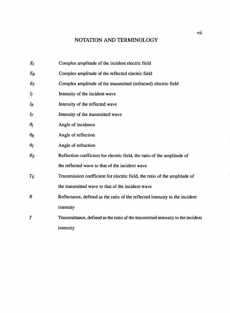
NOTATION AND TERMINOLOGY

Complex amplitude of the incident electric field

Complex amplitude of the reflected electric field

Complex amplitude of the transmitted (refracted) electric field

Intensity of the incident wave

Intensity of the reflected wave

Intensity of the transmitted wave

Angle of incidence

Angle of reflection

Angle of refraction

Reflection coefficient for electric field, the ratio of the amplitude of

the reflected wave to that of the incident wave

Transmission coefficient for electric field, the ratio of the amplitude of

the transmitted wave to that of the incident wave

Reflectance, defined as the ratio of the reflected intensity to the incident

intensity

Vll

Transmittance, defined as the ratio of the transmitted intensity to the incident

intensity

1

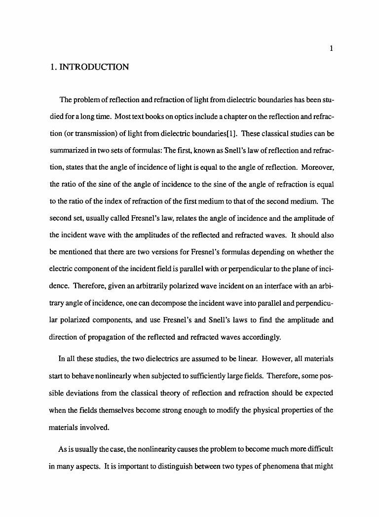
1. INTRODUCTION

The problem of reflection and refraction of light from dielectric boundaries has been stu­

died for a long time. Most text books on optics include a chapter on the reflection and refrac­

tion (or transmission) of light from dielectric boundaries[ 1 ]. These classical studies can be

summarized in two sets of formulas: The first, known as Snell's law of reflection and refrac­

tion, states that the angle of incidence of light is equal to the angle of reflection. Moreover,

the ratio of the sine of the angle of incidence to the sine of the angle of refraction is equal

to the ratio of the index of refraction of the first medium to that of the second medium. The

second set, usually called Fresnel's law, relates the angle of incidence and the amplitude of

the incident wave with the amplitudes of the reflected and refracted waves. It should also

be mentioned that there are two versions for Fresnel's formulas depending on whether the

electric component of the incident field is parallel with or perpendicular to the plane of inci­

dence. Therefore, given an arbitrarily polarized wave incident on an interface with an arbi­

trary angle of incidence, one can decompose the incident wave into parallel and perpendicu­

lar polarized components, and use Fresnel's and Snell's laws to find the amplitude and

direction of propagation of the reflected and refracted waves accordingly.

In all these studies, the two dielectrics are assumed to be linear. However, all materials

start to behave nonlinearly when subjected to sufficiently large fields. Therefore, some pos­

sible deviations from the classical theory of reflection and refraction should be expected

when the fields themselves become strong enough to modify the physical properties of the

materials involved.

As is usually the case, the nonlinearity causes the problem to become much more difficult

in many aspects. It is important to distinguish between two types of phenomena that might

2

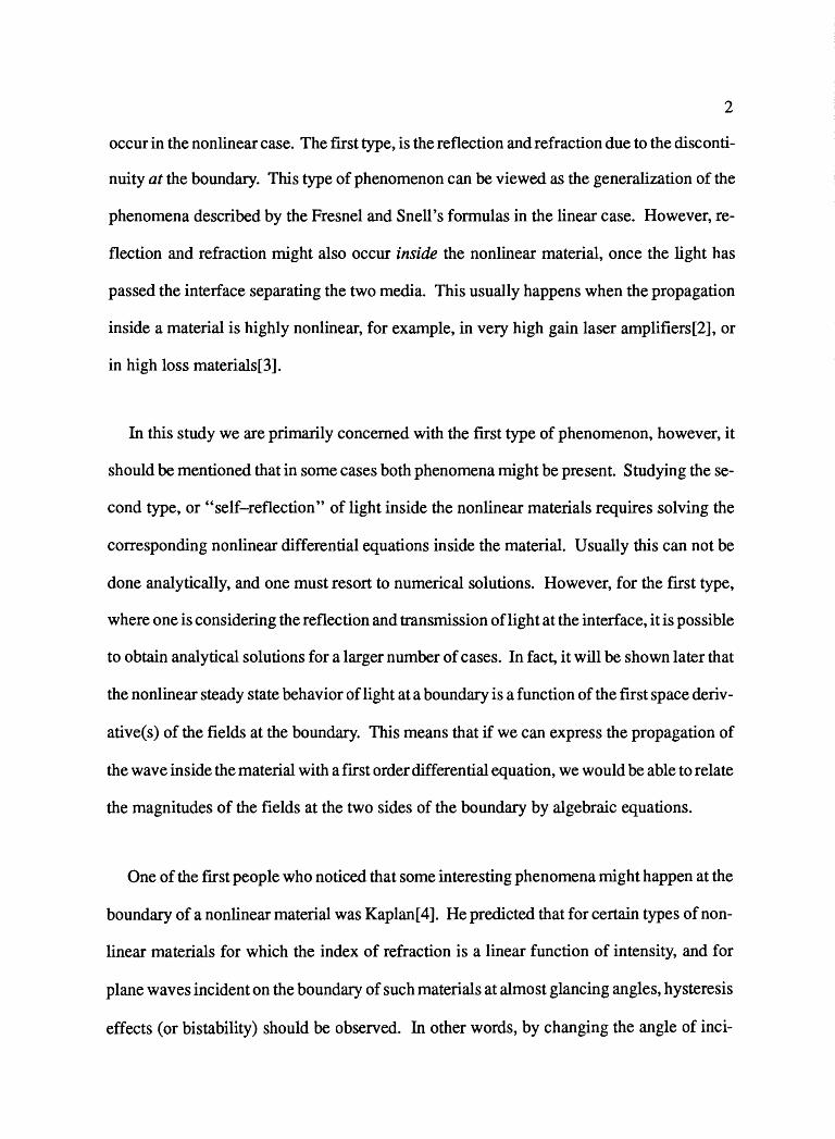
occur in the nonlinear case. The first type, is the reflection and refraction due to the disconti­

nuity at the boundary. This type of phenomenon can be viewed as the generalization of the

phenomena described by the Fresnel and Snell's formulas in the linear case. However, re­

flection and refraction might also occur inside the nonlinear material, once the light has

passed the interface separating the two media. This usually happens when the propagation

inside a material is highly nonlinear, for example, in very high gain laser amplifiers[2], or

in high loss materials[3].

In this study we are primarily concerned with the first type of phenomenon, however, it

should be mentioned that in some cases both phenomena might be present. Studying the se­

cond type, or "self-reflection" of light inside the nonlinear materials requires solving the

corresponding nonlinear differential equations inside the material. Usually this can not be

done analytically, and one must resort to numerical solutions. However, for the first type,

where one is considering the reflection and transmission oflight at the interface, it is possible

to obtain analytical solutions for a larger number of cases. In fact, it will be shown later that

the nonlinear steady state behavior oflight at a boundary is a function of the first space deriv­

ative(s) of the fields at the boundary. This means that if we can express the propagation of

the wave inside the material with a first order differential equation, we would be able to relate

the magnitudes of the fields at the two sides of the boundary by algebraic equations.

One of the first people who noticed that some interesting phenomena might happen at the

boundary of a nonlinear material was Kaplan[ 4]. He predicted that for certain types of non­

linear materials for which the index of refraction is a linear function of intensity, and for

plane waves incident on the boundary of such materials at almost glancing angles, hysteresis

effects (or bistability) should be observed. In other words, by changing the angle of inci-

3

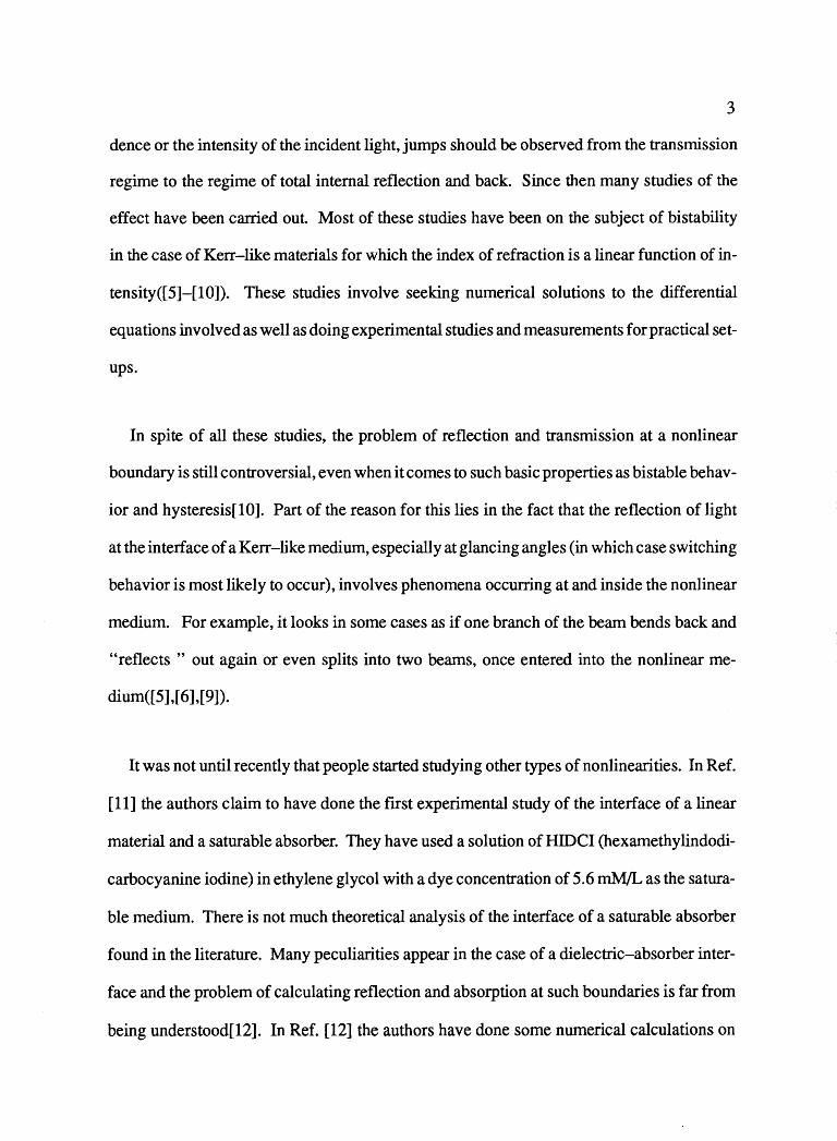
dence or the intensity of the incident light, jumps should be observed from the transmission

regime to the regime of total internal reflection and back. Since then many studies of the

effect have been carried out. Most of these studies have been on the subject of bistability

in the case of Kerr-like materials for which the index of refraction is a linear function of in­

tensity([ 5]-[ 10]). These studies involve seeking numerical solutions to the differential

equations involved as well as doing experimental studies and measurements for practical set­

ups.

In spite of all these studies, the problem of reflection and transmission at a nonlinear

boundary is still controversial, even when it comes to such basic properties as bistable behav­

ior and hysteresis[lO]. Part of the reason for this lies in the fact that the reflection of light

at the interface of a Kerr-like medium, especially at glancing angles (in which case switching

behavior is most likely to occur), involves phenomena occurring at and inside the nonlinear

medium. For example, it looks in some cases as if one branch of the beam bends back and

"reflects " out again or even splits into two beams, once entered into the nonlinear me-

di um([ 5] ,[ 6] ,[9]).

It was not until recently that people started studying other types of nonlinearities. In Ref.

[11] the authors claim to have done the first experimental study of the interface of a linear

material and a saturable absorber. They have used a solution of HIDCI (hexamethylindodi­

carbocyanine iodine) in ethylene glycol with a dye concentration of 5.6 mM/L as the satura­

ble medium. There is not much theoretical analysis of the interface of a saturable absorber

found in the literature. Many peculiarities appear in the case of a dielectric-absorber inter­

face and the problem of calculating reflection and absorption at such boundaries is far from

being understood[12]. In Ref. [12] the authors have done some numerical calculations on

4

this problem. They have not made the assumption of low gain per wave length, and therefore

they have used a second order differential equation for propagation of light inside the nonlin­

ear medium. Numerical solution of the differential equation inside the boundary and ap­

plication of the boundary conditions at the interface then results in nonlinear reflection coef­

ficients at the boundary, and self-reflection of light inside the nonlinear absorber.

This work is ordered as follows. First some necessary concepts are developed which will

be needed later in this study. These concepts include some mathematical relations and ex­

pressions which relate the electric and magnetic complex amplitudes of the wave inside the

nonlinear medium. Also an expression relating the intensity of the wave with the complex

amplitude of the electric field in the general nonlinear case is derived. These results will

prove to be useful later, because usually, one is interested in what happens to the intensity

of the wave upon reflection or transmission from the boundary. The complex amplitudes

of the fields which are not directly measurable quantities are usually of secondary impor­

tance. Also these expressions become handy in finding the magnetic component of the field

once the electric component is found.

Next, starting from Maxwell's equations and boundary conditions, a rather general for­

malism to handle the reflection and transmission of light from the interface between two ar­

bitrary nonlinear media is worked out. It is also shown that all the interesting physics in­

volved in the problem can be described by the space derivative(s) of the electric field at the

two sides of the boundary.

In the next two chapters some special cases of this general formalism are considered. As

the simplest special case, and also as a check on the theory, the limit where both media are

linear dielectrics will be discussed. In this way, the familiar Fresnel and Snell's laws will

5

be derived as special cases of the previous expressions. Then the case where one of the mate­

rials is a linear dielectric and the other one is a saturable absorber or amplifier is studied.

Here a low gain (loss) per wave length is assumed, which allows for using first order diff eren­

tial equations for the propagation of the waves inside the nonlinear material. While making

this assumption will probably result in the neglecting of some interesting phenomena, it en­

ables the expression of the space derivatives of the fields in terms of the fields themselves.

Thus it would be possible to obtain algebraic equations for the amplitudes of the fields at the

two sides of the boundary.

6

2. REFLECTION, REFRACTION, AND BOUNDARY CONDITIONS

2.1. PRELIMINARIES

One of the important aspects of propagation of electromagnetic waves in nonlinear media

is that unlike the linear case, there is not a simple relationship between the electric and mag­

netic components of the field. For example, in a very high gain laser amplifier the electric

and magnetic components of the wave might become partially decoupled. Moreover, each

might have a different "local" wavelength[2] or a different "instantaneous" frequency[13].

In the context of this study, we might be able to find the reflection coefficient for the electric

component of the wave, but we might also be interested to find the same coefficient for the

magnetic component of the wave. If we have an expression to relate the electric and magnet­

ic components of the waves in the general nonlinear case, our task would become simpler.

Once we find such an expression, we would also be able to express the intensity of the wave

in terms of the electric field. This is not obvious in the nonlinear case, and is of importance

to us because the intensity is the primary measurable quantity.

Usually the electric or magnetic field of an electromagnetic wave is represented as the

product of a slowly varying function of time and space and an exponential function which

represents the rapid periodic changes in time and space. Often times it becomes necessary

to integrate such expressions either with respect to time or space. Let us assume two arbitrary

complex functions F(z,t) andf(z,t) defined as:

F(z, t) = f (z, t) exp(ikz - iwt) (2.1)

In other words, we have assumed that/is the complex amplitude of F. It is possible to express

7

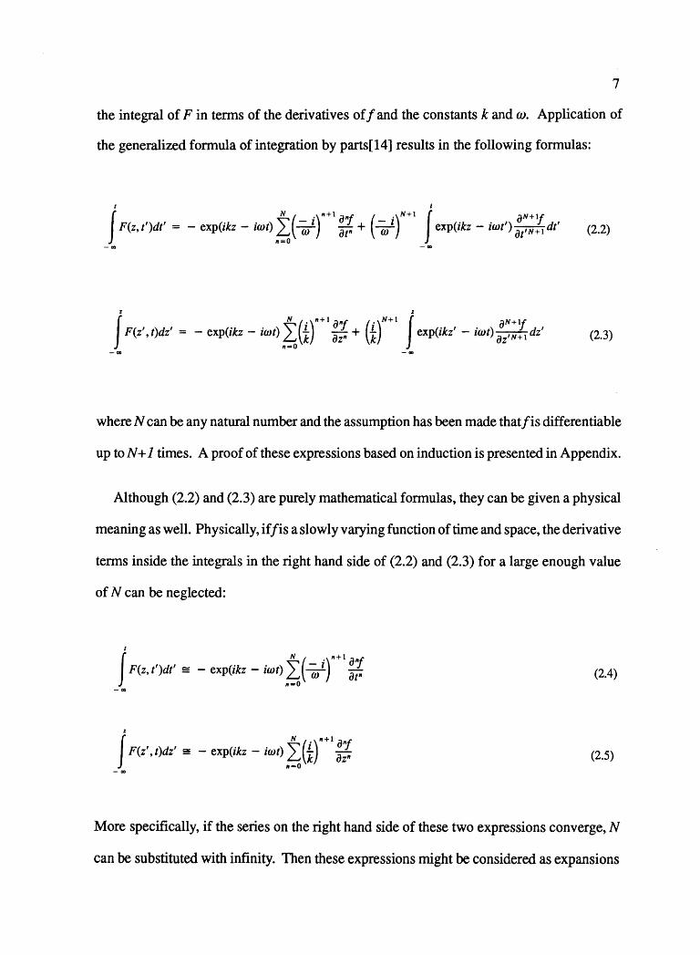
the integral of F in terms of the derivatives off and the constants k and w. Application of

the generalized formula of integration by parts[l4] results in the following formulas:

ft N (- .)11+1 iJ"f (- .)N+l ft iJN+1j F(z, t')dt' = - exp(ikz - iwt) L w 1 iJt11 + w 1

exp(ikz - iwt') iJt'N+l dt' 11=0

(2.2) -~ -~

fz N ( .)11+1 iJllf ( .)N+l fz iJN+1f F(z', t)dz' = - exp(ikz - iwt) I t iJz11 + t exp(ikz' - iwt) iJz'N+l dz'

11-=0 (2.3)

where N can be any natural number and the assumption has been made thatf is differentiable

up to N+ 1 times. A proof of these expressions based on induction is presented in Appendix.

Although (2.2) and (2.3) are purely mathematical formulas, they can be given a physical

meaning as well. Physically, if fis a slowly varying function of time and space, the derivative

terms inside the integrals in the right hand side of (2.2) and (2.3) for a large enough value

of N can be neglected:

ft N (- .)11+1 iJ"f F(z, t')dt' = - exp(ikz - iwt) ~ w 1 iJt11

fz N ( .)11+1 iJ"f F(z', t)dz' = - exp(ikz - iwt) L i az11

11•0 - DO

(2.4)

(2.5)

More specifically, if the series on the right hand side of these two expressions converge, N

can be substituted with infinity. Then these expressions might be considered as expansions

8

of the integral of a physical quantity (electric or magnetic field) in terms of the derivatives

of the complex amplitude of that quantity.

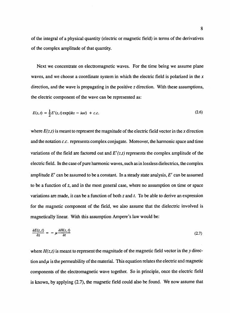
Next we concentrate on electromagnetic waves. For the time being we assume plane

waves, and we choose a coordinate system in which the electric field is polarized in the x

direction, and the wave is propagating in the positive z direction. With these assumptions,

the electric component of the wave can be represented as:

E(z, t) = !E'(z, t) exp(ikz - imt) + c.c. (2.6)

where E( z ,t) is meant to represent the magnitude of the electric field vector in the x direction

and the notation c.c. represents complex conjugate. Moreover, the harmonic space and time

variations of the field are factored out and E' (z,t) represents the complex amplitude of the

electric field. In the case of pure harmonic waves, such as in lossless dielectrics, the complex

amplitude E' can be assumed to be a constant. In a steady state analysis, E' can be assumed

to be a function of z, and in the most general case, where no assumption on time or space

variations are made, it can be a function of both z and t. To be able to derive an expression

for the magnetic component of the field, we also assume that the dielectric involved is

magnetically linear. With this assumption Ampere's law would be:

iJE(z, t) iJH(z, t) -az- = - µ-a-t- (2.7)

where H(z,t) is meant to represent the magnitude of the magnetic field vector in they direc-

tion andµ is the permeability of the material. This equation relates the electric and magnetic

components of the electromagnetic wave together. So in principle, once the electric field

is known, by applying (2.7), the magnetic field could also be found. We now assume that

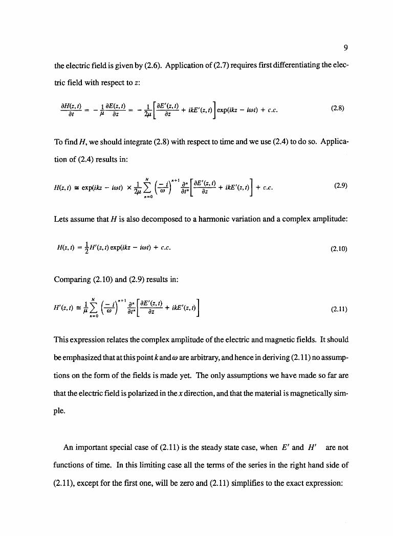
9

the electric field is given by (2.6). Application of (2.7) requires first differentiating the elec-

tric field with respect to z:

iJH(z, t) = _ l iJE(z, t) = _ L [iJE~(z, t) + ikE'(z, t)] exp(ikz - iwt) + c.c. at µ (Jz ~ z

(2.8)

To findH, we should integrate (2.8) with respect to time and we use (2.4) to do so. Applica-

tion of (2.4) results in:

H(z, t) "' exp(ikz - iwt) X ~ ~0 ( ~ f 1

;1: [OE~~· t) + ikE'(z, t)] + c.c. (2.9)

Lets assume that H is also decomposed to a harmonic variation and a complex amplitude:

H(z, t) = ! H' (z, t) exp(ikz - iwt) + c .c. (2.10)

Comparing (2.10) and (2.9) results in:

H'(z, t) " fr i: ( ~ f 1

:;. [iJE~~' t) + ikE'(z, t)] n"'O

(2.11)

This expression relates the complex amplitude of the electric and magnetic fields. It should

be emphasized that at this point k andm are arbitrary, and hence in deriving (2.11) no assump-

tions on the form of the fields is made yet. The only assumptions we have made so far are

that the electric field is polarized in the x direction, and that the material is magnetically sim-

ple.

An important special case of (2.11) is the steady state case, when E' and H' are not

functions of time. In this limiting case all the terms of the series in the right hand side of

(2.11 ), except for the first one, will be zero and (2.11) simplifies to the exact expression:

10

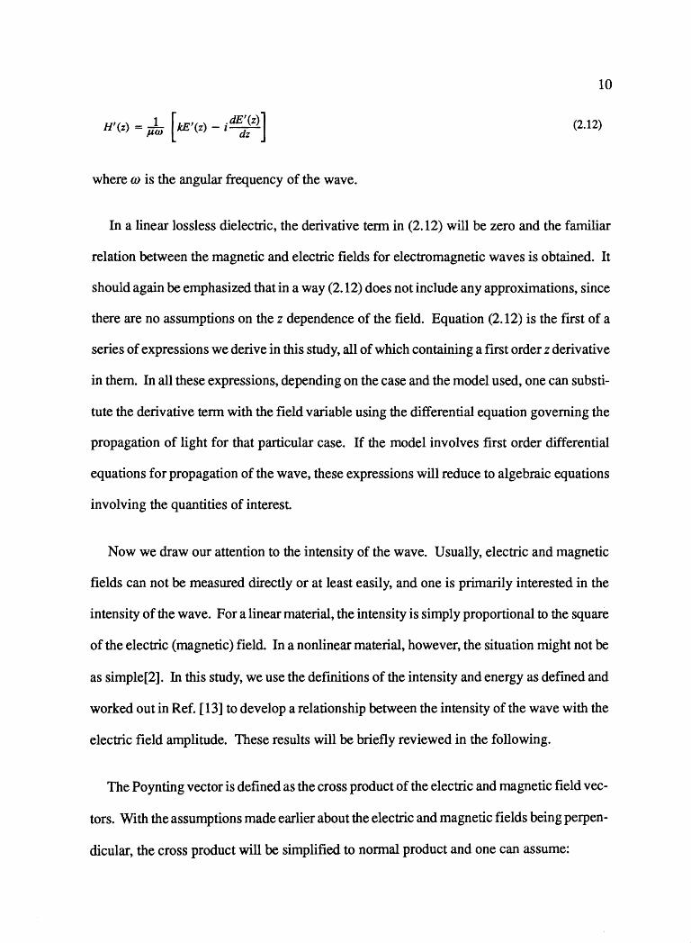
H'(z) = µ~ [ kE'(z) _ /lE,;;z)] (2.12)

where w is the angular frequency of the wave.

In a linear lossless dielectric, the derivative term in (2.12) will be zero and the familiar

relation between the magnetic and electric fields for electromagnetic waves is obtained. It

should again be emphasized that in a way (2.12) does not include any approximations, since

there are no assumptions on the z dependence of the field. Equation (2.12) is the first of a

series of expressions we derive in this study, all of which containing a first order z derivative

in them. In all these expressions, depending on the case and the model used, one can substi-

tute the derivative term with the field variable using the differential equation governing the

propagation of light for that particular case. If the model involves first order differential

equations for propagation of the wave, these expressions will reduce to algebraic equations

involving the quantities of interest

Now we draw our attention to the intensity of the wave. Usually, electric and magnetic

fields can not be measured directly or at least easily, and one is primarily interested in the

intensity of the wave. For a linear material, the intensity is simply proportional to the square

of the electric (magnetic) field. In a nonlinear material, however, the situation might not be

as simple[2]. In this study, we use the definitions of the intensity and energy as defined and

worked out in Ref. [13] to develop a relationship between the intensity of the wave with the

electric field amplitude. These results will be briefly reviewed in the following.

The Poynting vector is defined as the cross product of the electric and magnetic field vec-

tors. With the assumptions made earlier about the electric and magnetic fields being perpen-

dicular, the cross product will be simplified to normal product and one can assume:

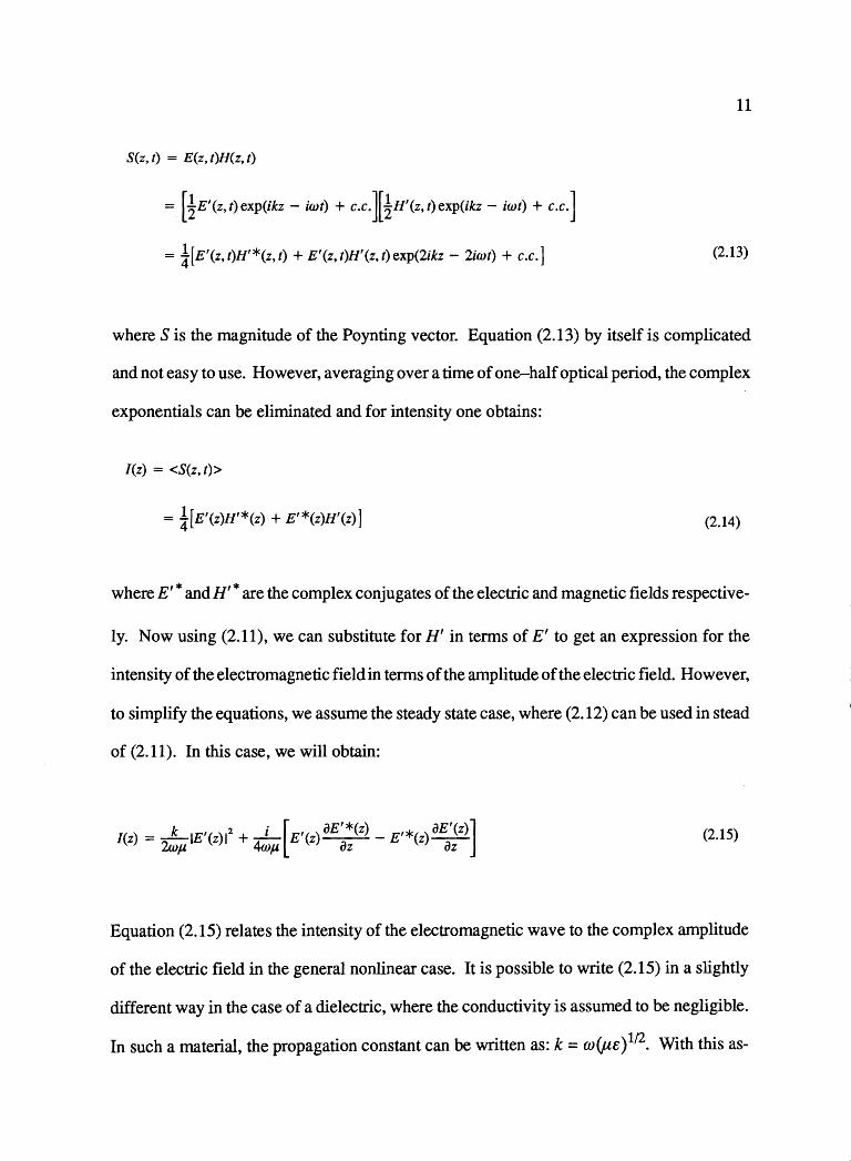
11

S{z, t) = E(z, t)H(z, t)

= [!E'(z,t)exp(ikz - iwt) + c.c.][!H'(z,t)exp(ikz - iwt) + c.c.]

= i[E'(z, t)H'*(z, t) + E'(z, t)H'(z, t) exp(2ikz - 2iwt) + c.c.] (2.13)

where S is the magnitude of the Poynting vector. Equation (2.13) by itself is complicated

and not easy to use. However, averaging over a time of one-half optical period, the complex

exponentials can be eliminated and for intensity one obtains:

I(z) = <S(z, t)>

= i[E'(z)H'*(z) + E'*(z)H'(z)] (2.14)

where E' *and H' *are the complex conjugates of the electric and magnetic fields respective-

ly. Now using (2.11), we can substitute for H' in terms of E' to get an expression for the

intensity of the electromagnetic field in terms of the amplitude of the electric field. However,

to simplify the equations, we assume the steady state case, where (2.12) can be used in stead

of (2.11). In this case, we will obtain:

I(z) = ~ IE'(z)l2 + _z_· [E'(z) iJE'*(z) - E'*( ) iJE'(z)] µ 4wµ az z az

(2.15)

Equation (2.15) relates the intensity of the electromagnetic wave to the complex amplitude

of the electric field in the general nonlinear case. It is possible to write (2.15) in a slightly

different way in the case of a dielectric, where the conductivity is assumed to be negligible.

In such a material, the propagation constant can be written as: k = w(µe )112. With this as-

12

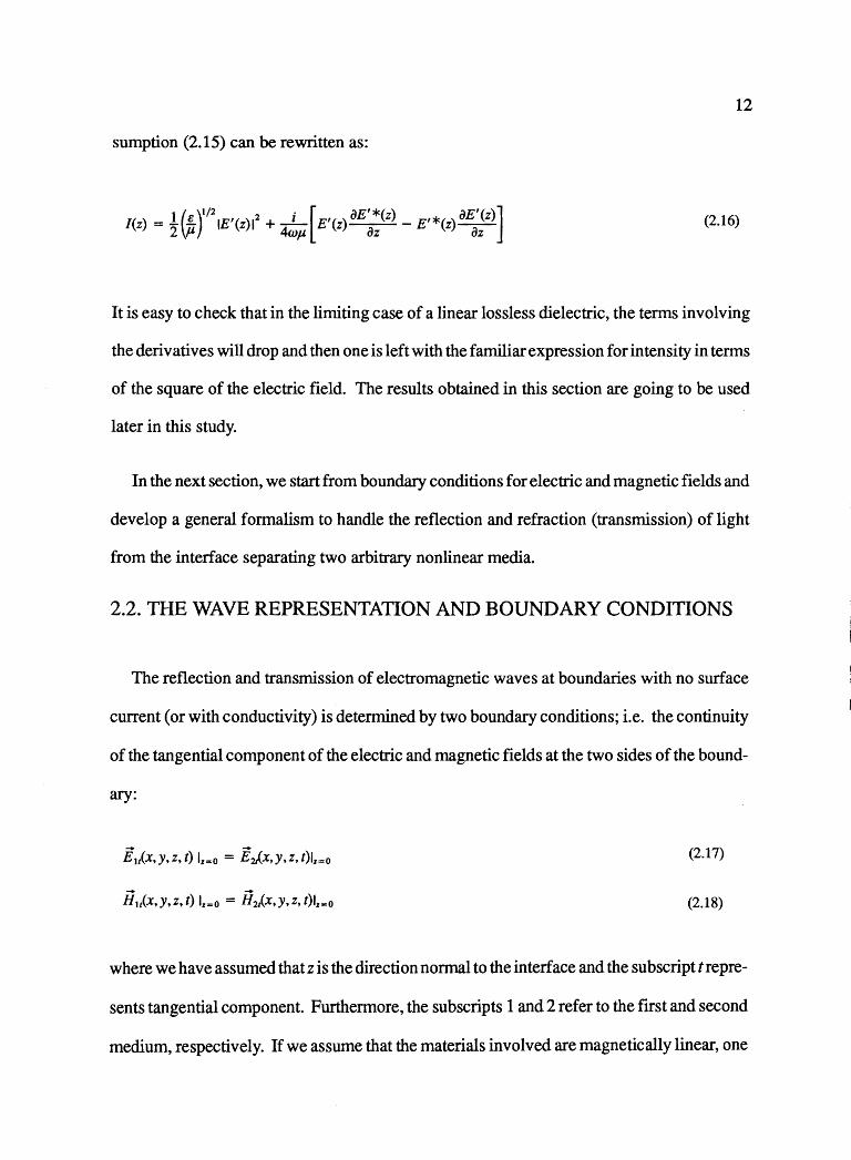
sumption (2.15) can be rewritten as:

I(z) = !(!.)1121E'(z)l2 +-1-· [E'(z) CJE'*(z) - E'*( )aE'(z)]

2 µ 4wµ az z az (2.16)

It is easy to check that in the limiting case of a linear lossless dielectric, the terms involving

the derivatives will drop and then one is left with the familiar expression for intensity in terms

of the square of the electric field. The results obtained in this section are going to be used

later in this study.

In the next section, we start from boundary conditions for electric and magnetic fields and

develop a general formalism to handle the reflection and refraction (transmission) of light

from the interface separating two arbitrary nonlinear media.

2.2. THE WAVE REPRESENTATION AND BOUNDARY CONDITIONS

The reflection and transmission of electromagnetic waves at boundaries with no surface

current (or with conductivity) is determined by two boundary conditions; i.e. the continuity

of the tangential component of the electric and magnetic fields at the two sides of the bound-

ary:

E11(x, y, z, t) 1.r-o = Eu(x, y, z, t)l.r=o (2.17)

H11(X,y,z,t) 1.r=O = H2l_x,y,z, t)l1 ... o (2.18)

where we have assumed that z is the direction normal to the interface and the subscript t repre-

sents tangential component. Furthermore, the subscripts 1 and 2 refer to the first and second

medium, respectively. If we assume that the materials involved are magnetically linear, one

13

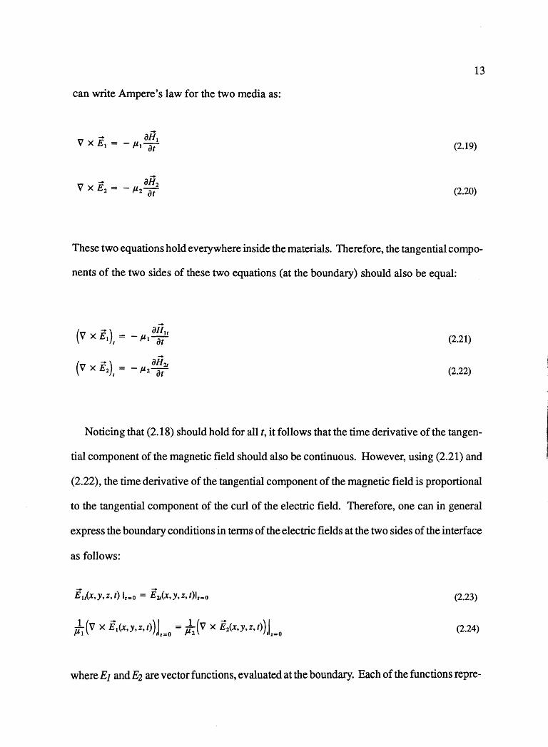
can write Ampere's law for the two media as:

... aii1 V X Ei = - µiTt (2.19)

... ... 0H2

V x E 2 = - µ2Tf (2.20)

These two equations hold everywhere inside the materials. Therefore, the tangential compo-

nents of the two sides of these two equations (at the boundary) should also be equal:

... (

... ) 0H11 V x E = -µi-1 t i)t (2.21)

... ) aiiu (v x E2 , = - µ2-af (2.22)

Noticing that (2.18) should hold for all t, it follows that the time derivative of the tangen-

tial component of the magnetic field should also be continuous. However, using (2.21) and

(2.22), the time derivative of the tangential component of the magnetic field is proportional

to the tangential component of the curl of the electric field. Therefore, one can in general

express the boundary conditions in terms of the electric fields at the two sides of the interface

as follows:

E1,(x,y,z,t) 1,,..0 = E21(x,y,z,t)l, ... o (2.23)

µ1 (v x E1(x,y,z,t)) I = µ1 (v x E2(x,y,z,t)) I

1 tz=O 2 tz=O (2.24)

where E1 and E2 are vector functions, evaluated at the boundary. Each of the functions repre-

14

sents the total electric field inside each of the materials and the subscript t represents tangen-

tial component.

In a way (2.23) and (2.24) are the most general form of the boundary conditions in terms

of the electric fields. Nevertheless, we are primarily interested in waves. In particular, we

want to consider a beam of light incident on the interface from the first medium, resulting

a reflected beam in the first medium and a transmitted beam in the second medium. To ac-

complish this we should adopt a more specific form for the electric field.

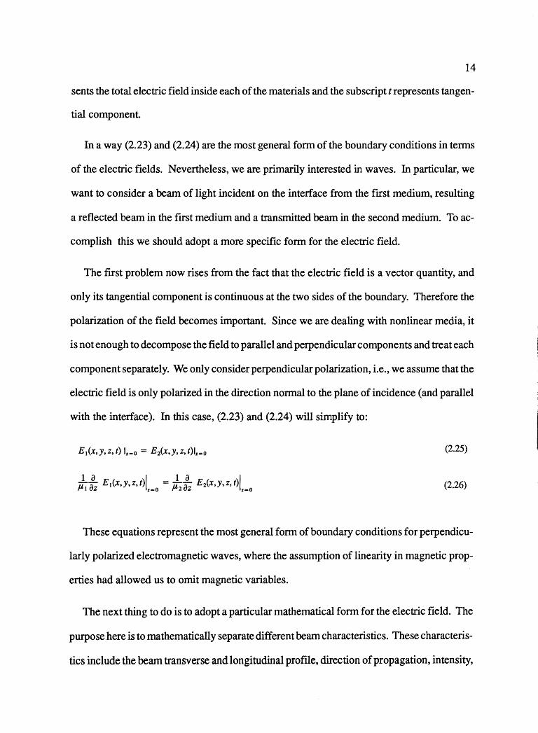
The first problem now rises from the fact that the electric field is a vector quantity, and

only its tangential component is continuous at the two sides of the boundary. Therefore the

polarization of the field becomes important. Since we are dealing with nonlinear media, it

is not enough to decompose the field to parallel and perpendicular components and treat each

component separately. We only consider perpendicular polarization, i.e., we assume that the

electric field is only polarized in the direction normal to the plane of incidence (and parallel

with the interface). In this case, (2.23) and (2.24) will simplify to:

E 1(x,y,z,t) lz=o = E2(x,y,z,t)l1 • 0 (2.25)

1 a I 1 a I µ-!! E1(x,y,z,t) = µ-!! E2(x,y,z,t) 1 uZ z=O 2 uZ z=O (2.26)

These equations represent the most general form of boundary conditions for perpendicu-

larly polarized electromagnetic waves, where the assumption of linearity in magnetic prop-

erties had allowed us to omit magnetic variables.

The next thing to do is to adopt a particular mathematical form for the electric field. The

purpose here is to mathematically separate different beam characteristics. These characteris-

tics include the beam transverse and longitudinal profile, direction of propagation, intensity,

15

etc. Once a particular mathematical representation for the beam is adopted, substituting it

into (2.25) and (2.26) results in the necessary relations to find the characteristics of the re­

flected and transmitted beams.

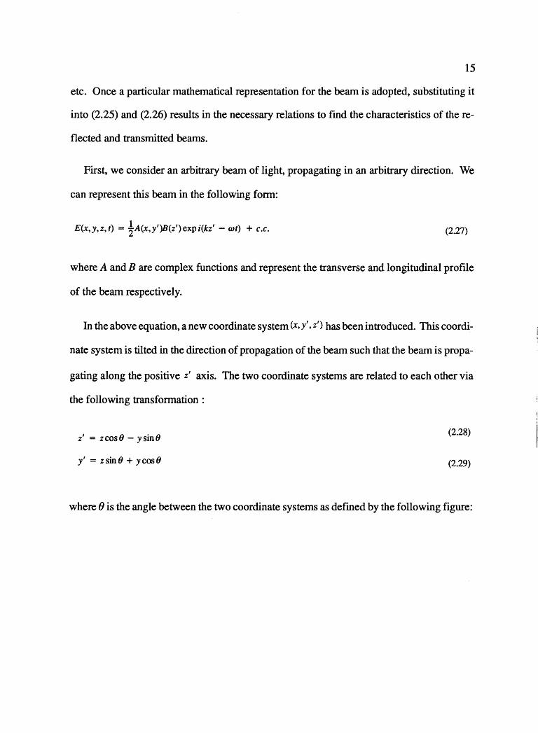
First, we consider an arbitrary beam of light, propagating in an arbitrary direction. We

can represent this beam in the following form:

E(x,y,z,t) = !A(x,y')B(z')expi(kz' - wt) + c.c. (2.27)

where A and B are complex functions and represent the transverse and longitudinal profile

of the beam respectively.

In the above equation, a new coordinate system (x, y'. z') has been introduced. This coordi­

nate system is tilted in the direction of propagation of the beam such that the beam is propa-

gating along the positive z' axis. The two coordinate systems are related to each other via

the following transformation :

z' = zcos8 - ysin8

y' = zsin8 + ycos8

(2.28)

(2.29)

where (} is the angle between the two coordinate systems as defined by the following figure:

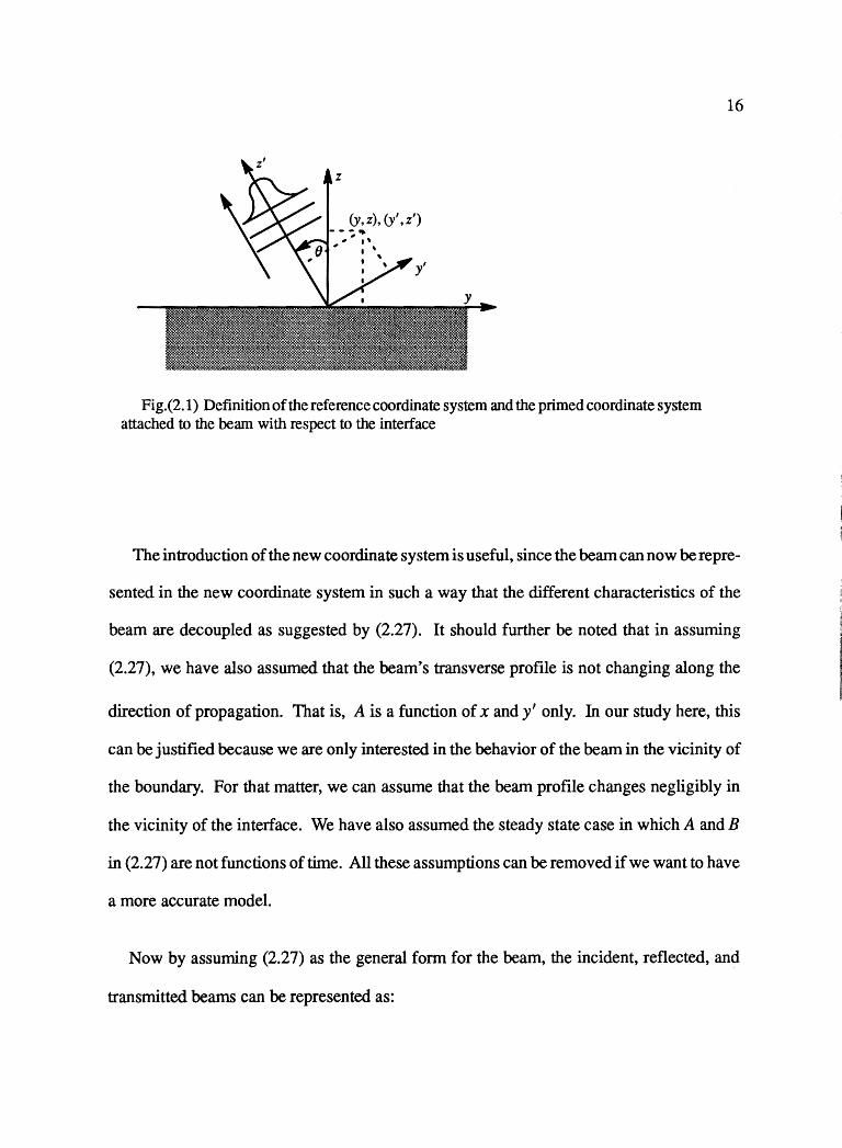
(y,z), (y' ,z')

Fig.(2.1) Definition of the reference coordinate system and the primed coordinate system attached to the beam with respect to the interface

16

The introduction of the new coordinate system is useful, since the beam can now be repre-

sented in the new coordinate system in such a way that the different characteristics of the

beam are decoupled as suggested by (2.27). It should further be noted that in assuming

(2.27), we have also assumed that the beam's transverse profile is not changing along the

direction of propagation. That is, A is a function of x and y' only. In our study here, this

can be justified because we are only interested in the behavior of the beam in the vicinity of

the boundary. For that matter, we can assume that the beam profile changes negligibly in

the vicinity of the interface. We have also assumed the steady state case in which A and B

in (2.27) are not functions of time. All these assumptions can be removed if we want to have

a more accurate model.

Now by assuming (2.27) as the general form for the beam, the incident, reflected, and

transmitted beams can be represented as:

17

Ei(_x,y, z, t) = !Ai(_x,y')Bi(z') expi(k1z' - wt) + c.c. (2.30)

E R(x, y, z, t) = ! AR(x, y')B R(z') exp i(k1z' - wt) + c .c. (2.31)

Ei(_x,y, z, t) = !Art.x,y')Bi(_z') exp i(k2z' - wt) + c.c. (2.32)

where the subscripts/, R, and T represent the incident, reflected, and transmitted beams re­

spectively. It should be mentioned that in each of these equations, the primed coordinate

system is with reference to the beam itself. Hence, each primed coordinate system is differ­

ent from the primed coordinate system used to represent another beam. Therefore, for each

of the equations (2.30), (2.31), and (2.32), the coordinate system (x,y',z') is related to the

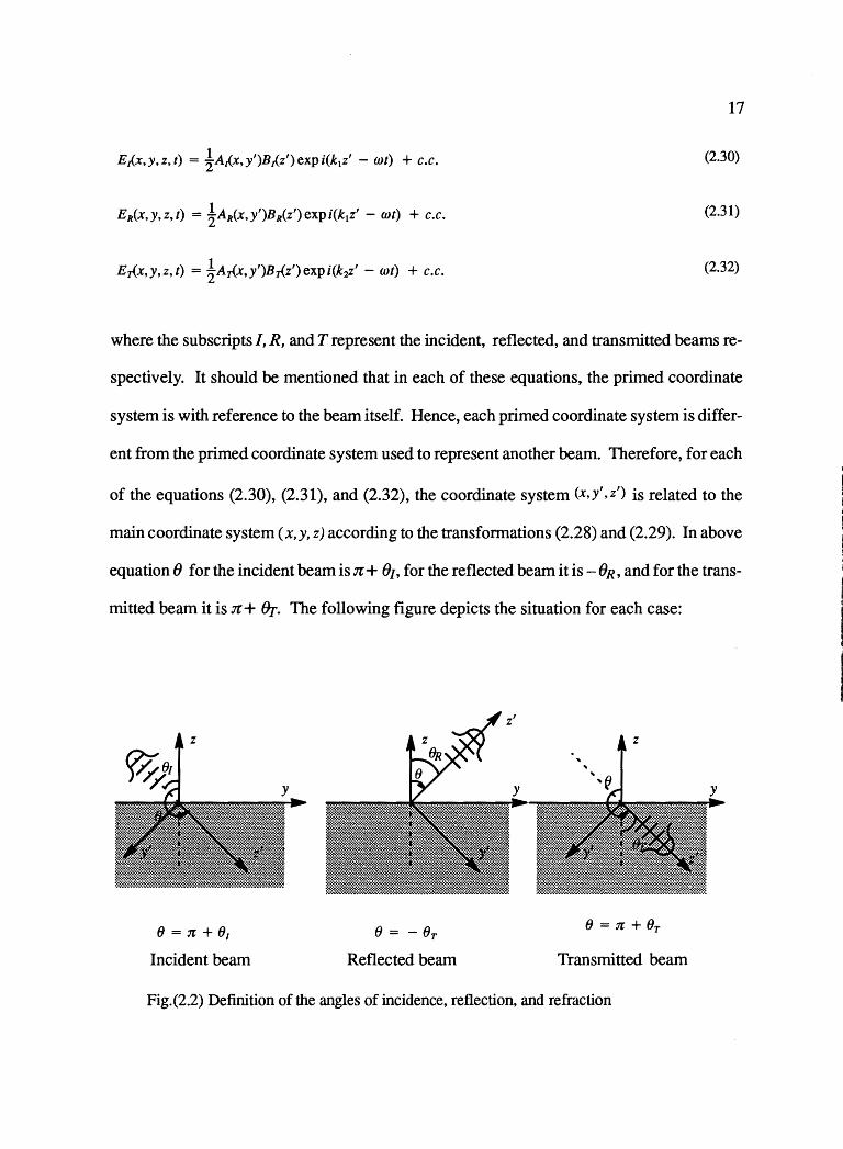
main coordinate system (x,y, z) according to the transformations (2.28) and (2.29). In above

equation (J for the incident beam is n + 01, for the reflected beam it is - (JR, and for the trans­

mitted beam it is n + &r. The following figure depicts the situation for each case:

(J = :re + 81

Incident beam

(J = - (JT

Reflected beam

(J = 1C + (JT

Transmitted beam

Fig.(2.2) Definition of the angles of incidence, reflection, and refraction

18

Also it should be noted that at this point we have not necessarily assumed that the angle of

incidence is equal to the angle of reflection.

The next step is to apply the boundary conditions (2.25) and (2.26) using the beam repre­

sentation just introduced. Using (2.25), one will obtain:

Ei(x,y,z, t)lz=O + ER(x,y,z, t)lz=O = Ei{x,y,z, t)lz=O (2.33)

And substituting from(2.30)-(2.32) and cancelling the exp(iw) terms from both sides of the

equation, one obtains:

A.r(.x,y')Bi(z')expi(k1z')l1

= 0 + Aix,y')Biz')expi(k1z')l1

= 0 = A:r(x,y')Br(z')expi(k2z')l1

... 0 (2.34)

However, one should remember that the primed coordinates used in (2.34) are relative to the

beams themselves. In each case the beam is propagating along the positive z' direction of

that coordinate system, furthermore, these coordinates are not the same in the incident, re­

flected, and transmitted beams. Therefore the next step is to write (2.34) with respect to the

"absolute" coordinate system which is attached to the interface. In doing so, the transforma:..

tions (2.28) and (2.29) can be used, replacing (} in each of the beams with the appropriate

angle, i.e., the angle between the beam and the normal to the interface:

Ai(x, - ycos 81)Bjy sin81) exp i(k1Y sin81)l1 = 0 + Aix,y cos 8R)B R(y sin 8R) exp i(k1y sin 8R)lz=o

= A:r(x, - ycos8T)B:r(ysin8T)expi(k2Jsin8T)lz=o

(2.35)

where the substitution z=O was made wherever z had appeared explicitly.

19

This equation relates the characteristics of the incident beam with those of the reflected

and transmitted beams. In the linear theory of reflection of plane waves from dielectric me­

dia, all the A and B functions in the above equation are simply constants. Therefore, one is

left with the exponential terms and the only way to satisfy (2.35) for all x and y is to require:

k1ysin01 = k1ysin0R = ki}'sinOT (2.36)

which is Snell's law of reflection and refraction stating the fact that the angle of incidence

is equal to the angle of reflection, and the ratio of the angle of incidence to the angle of refrac­

tion is equal to the ratio of the indices of refraction of the two media.

It is evident from (2.35) that in the general nonlinear case the above condition might not

be the case. In fact, the only thing one can say at this point is:

Br(y sin01) exp i(k1y sin 01) + BR(y sin OR) exp i(k1y sin OR) = B:r(y sin OT) exp i(kiY sin OT) (2.37)

In other words, the phase expressions which contain the angles are now coupled with the gain

expressions. It is worth asking that under what conditions it is possible to deduce (2.36) from

(2.37). One possible answer might be related to how fast the amplitude terms in (2.37) vary

with distance. The exponential terms in (2.37) are periodic functions changing in distances

of the order of the wavelength. On the other hand, the B functions in (2.37) which represent

the amplitude of the wave along the surface are usually slowly varying functions. Therefore,

it seems one can reach at the following conclusion : If the gain or loss is small enough so that

the amplitude of the wave changes negligibly in a wavelength, it is possible to deduce (2.36)

from (2.37) ,i.e., Snell's law of reflection and refraction holds. If this assumption is not true,

20

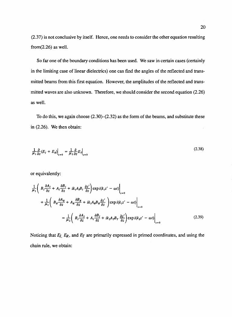
(2.37) is not conclusive by itself. Hence, one needs to consider the other equation resulting

from(2.26) as well.

So far one of the boundary conditions has been used. We saw in certain cases (certainly

in the limiting case of linear dielectrics) one can find the angles of the reflected and trans-

mitted beams from this first equation. However, the amplitudes of the reflected and trans-

mitted waves are also unknown. Therefore, we should consider the second equation (2.26)

as well.

To do this, we again choose (2.30)-(2.32) as the form of the beams, and substitute these

in (2.26). We then obtain:

1 o I 1 o tj --(E1 + ER) = --E µ1 OZ .r•O µ2 OZ .r-0

(2.38)

or equivalently:

1 ( B aAr A oB I .k A "R oz') .(k I )I µ1 ITz + ITz + l 1 JL'l az expz 1Z - Wt z=O

1 ( oAR A aBR .k A B oz' ) .(k , )I + µ1 BRTz + RTz + l 1 R RTz expz 1Z - wt z=O

1 ( aAr A oBr .k A oz') .(k I )I = µ2 Br-az + ITz + l PiBr Tz expz 2Z - wt z=O

(2.39)

Noticing that E1, ER, and Er are primarily expressed in primed coordinates, and using the

chain rule, we obtain:

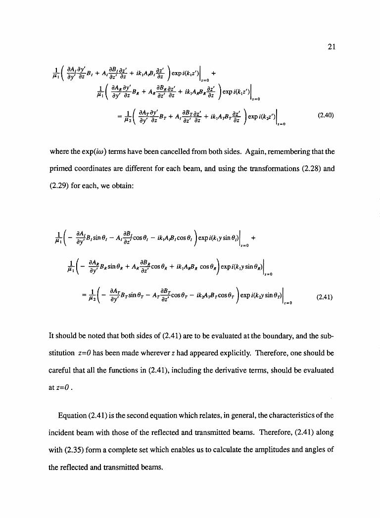
21

J_( oA1oy' B +A 0B1oz' + ik A!J oz' ) expi(k1z')I +

µ1 oy' OZ I I oz' OZ l I OZ z=O

J_ ( oAR oy' B + A oB Roz' + ik A B oz' ) exp i(k1z')I µ1 oy' OZ R R oz' OZ 1 R R OZ z=O

_ 1 ( oAToy' oBToz' . oz' ) I - µ2 ay' a;BT + A1 oz' Tz + lk1A1'1TTz exp i(k2z') z=O (2.40)

where the exp(iw) terms have been cancelled from both sides. Again, remembering that the

primed coordinates are different for each beam, and using the transformations (2.28) and

(2.29) for each, we obtain:

J1 (- ~A:B1 sin01 - A1 :~,1cos01 - ik1A/J1cos01 )expi(k1ysin01)I + y z=O

J1(- O::BRsinOR +AR ~~~cos(JR + ik1ARBR coseR)expi(k1ysinOR)I y z=O

= µ1 (- oA; BT sin OT - AT :B; cos OT - ik-ifiiBTcosOT) exp i(k2Y sinOT)I (2 41) 2 oy vZ z=O •

It should be noted that both sides of (2.41) are to be evaluated at the boundary, and the sub-

stitution z=O has been made wherever z had appeared explicitly. Therefore, one should be

careful that all the functions in (2.41 ), including the derivative terms, should be evaluated

at z=O.

Equation (2.41) is the second equation which relates, in general, the characteristics of the

incident beam with those of the reflected and transmitted beams. Therefore, (2.41) along

with (2.35) form a complete set which enables us to calculate the amplitudes and angles of

the reflected and transmitted beams.

22

Considering (2.41) carefully reveals that the reflection and transmission characteristics

of the beam are related to:

1) The amplitudes of the beams at the boundary;

2) The derivative of the transverse profile of the beam along the direction perpendicular; to

the direction of the propagation at the boundary. Obviously, this is a consequent of the beam

(transverse) profile inside the boundary;

3) The derivative of the longitudinal profile of the beam along the direction of the propaga­

tion at the boundary. Of course, this is again the propagation characteristic of the beam inside

either medium, and is a result of the solution of the nonlinear wave equation inside either

medium;

4) The angle of propagation of the beam with respect to the interface.

Again it should be emphasized that in general (2.41) and (2.35) should be considered to­

gether. Using them, one should be able to calculate the amplitudes and angles of propagation

of the reflected and transmitted beams, given the amplitude and angle of propagation of the

input beam and the propagation characteristics for beams inside both media close to the in­

terface. It is clear that(2.41) and (2.35) are in general coupled, and one can not simply deduce

Snell's law for the angles of propagation of the beams, as would be the case with the limiting

case of linear dielectrics.

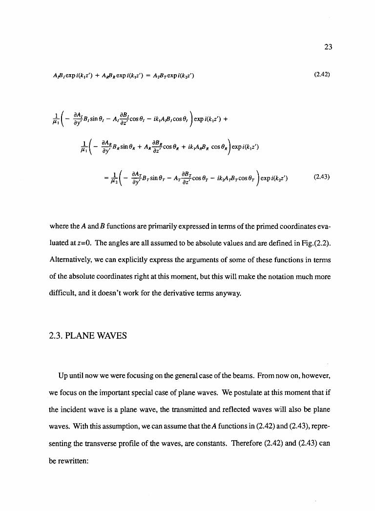
In conclusion, in this section we obtained two general equations. In this way, given the

amplitude and angle of the incident beam, one should be able to calculate those of the re­

flected and transmitted beams. For further reference we rewrite these two equations together

again.

23

Aj11expi(k1z') + AaBRexpi(k1z') = ArBTexpi(k2z') (2.42)

J, (- :~{B1 sin81 -A, :!:cos81 - ik1A,B1 cos81 )expi(k1z') +

J, ( - :~~ B •sin 8 • + A, :~~cos 8, + ik1A,,B • cos 8 •)exp i(k1z')

_ 1 ( aAT . aB T . ) - µ

2 - ay' BT sm 9T - AT oz' cos 9T - zk-iAifJ Tcos eT exp i(k2z') (2.43)

where the A andB functions are primarily expressed in terms of the primed coordinates eva­

luated at z=O. The angles are all assumed to be absolute values and are defined in Fig.(2.2).

Alternatively, we can explicitly express the arguments of some of these functions in terms

of the absolute coordinates right at this moment, but this will make the notation much more

difficult, and it doesn't work for the derivative terms anyway.

2.3. PLANE WAVES

Up until now we were focusing on the general case of the beams. From now on, however,

we focus on the important special case of plane waves. We postulate at this moment that if

the incident wave is a plane wave, the transmitted and reflected waves will also be plane

waves. With this assumption, we can assume that the A functions in (2.42) and (2.43), repre­

senting the transverse profile of the waves, are constants. Therefore (2.42) and (2.43) can

be rewritten:

A!J h') exp i(k1z') + ARB R(z') exp i(k1z') = A~ :r(z') exp i(k2z')

J, ( - A, a~~;'> coslJ1 - ik1A/Jh')coslJ,) expi(k,z') +

J, (A. a~';;') cos IJ • + ik,A,!J .~') cos IJ •) exp i(k,z')

= J2

( - Ar aBf,;'> cos Or - ik,A,B,{z')coslJr) expi(k,z')

24

(2.44)

(2.45)

The above equations, not being with reference to one single coordinate system, are not very

useful. Therefore, we should express these equations in terms of the absolute coordinate sys­

tem. Using the transformations (2.28) and (2.29), and with appropriate choice of() for each

case, we will obtain:

A1Bi()'sin01)expi(k1ysin01) + ARBR(ysinOR)expi(k1ysinOR) = AJJ:r(ysinOT)expi(k2)'sinOT)

(2.46)

J, cos o{ -A/8 j,;'> - ik,A/l ,(y sin IJ ,) ) exp i(k1y sin IJ 1) +

;, cos IJ •(A• a Ba:~') + ik1A•B .(y sin IJ .) ) exp i(k,y sin IJ•)

= J2 cos Br( - Ar aBa~;'> - ik,A,B.,{y sin Br) ) exp i(k,y sin Br) (2.47)

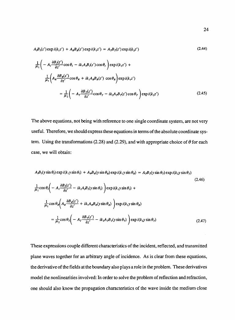
These expressions couple different characteristics of the incident, reflected, and transmitted

plane waves together for an arbitrary angle of incidence. As is clear from these equations,

the derivative of the fields at the boundary also plays a role in the problem. These derivatives

model the nonlinearities involved: In order to solve the problem of reflection and refraction,

one should also know the propagation characteristics of the wave inside the medium close

25

to the boundary. In general this requires solving the nonlinear wave equation in either me­

dium. So in a way the problem of nonlinear reflection and refraction of light is reduced to

nonlinear propagation of light. However, in some cases these derivatives can be expressed

without having to solve the nonlinear wave equation. This can be done when the wave equa­

tion governing the propagation of light in the medium is of first order.

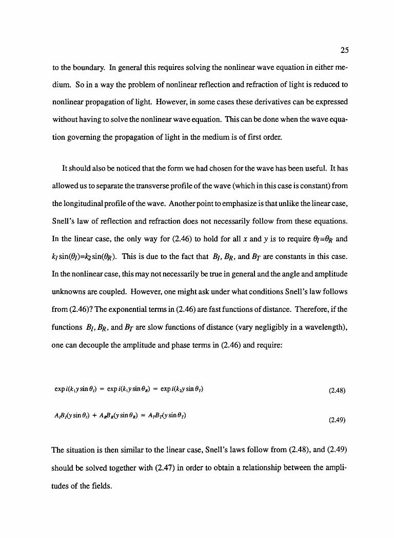
It should also be noticed that the form we had chosen for the wave has been useful. It has

allowed us to separate the transverse profile of the wave (which in this case is constant) from

the longitudinal profile of the wave. Another point to emphasize is that unlike the linear case,

Snell's law of reflection and refraction does not necessarily follow from these equations.

In the linear case, the only way for (2.46) to hold for all x and y is to require 01=0R and

ki sin(01)=k2 sin( OR). This is due to the fact that B1, BR, and BT are constants in this case.

In the nonlinear case, this may not necessarily be true in general and the angle and amplitude

unknowns are coupled. However, one might ask under what conditions Snell's law follows

from (2.46)? The exponential terms in (2.46) are fast functions of distance. Therefore, if the

functions B1, BR, andBT are slow functions of distance (vary negligibly in a wavelength),

one can decouple the amplitude and phase terms in (2.46) and require:

expi(k1ysin81) = expi(k1ysin8R) = expi(k2,}'sin8T) (2.48)

A1Bhsin81) + AJ1R(ysin8R) = AiBT(ysinOT) (2.49)

The situation is then similar to the linear case, Snell's laws follow from (2.48), and (2.49)

should be solved together with (2.47) in order to obtain a relationship between the ampli­

tudes of the fields.

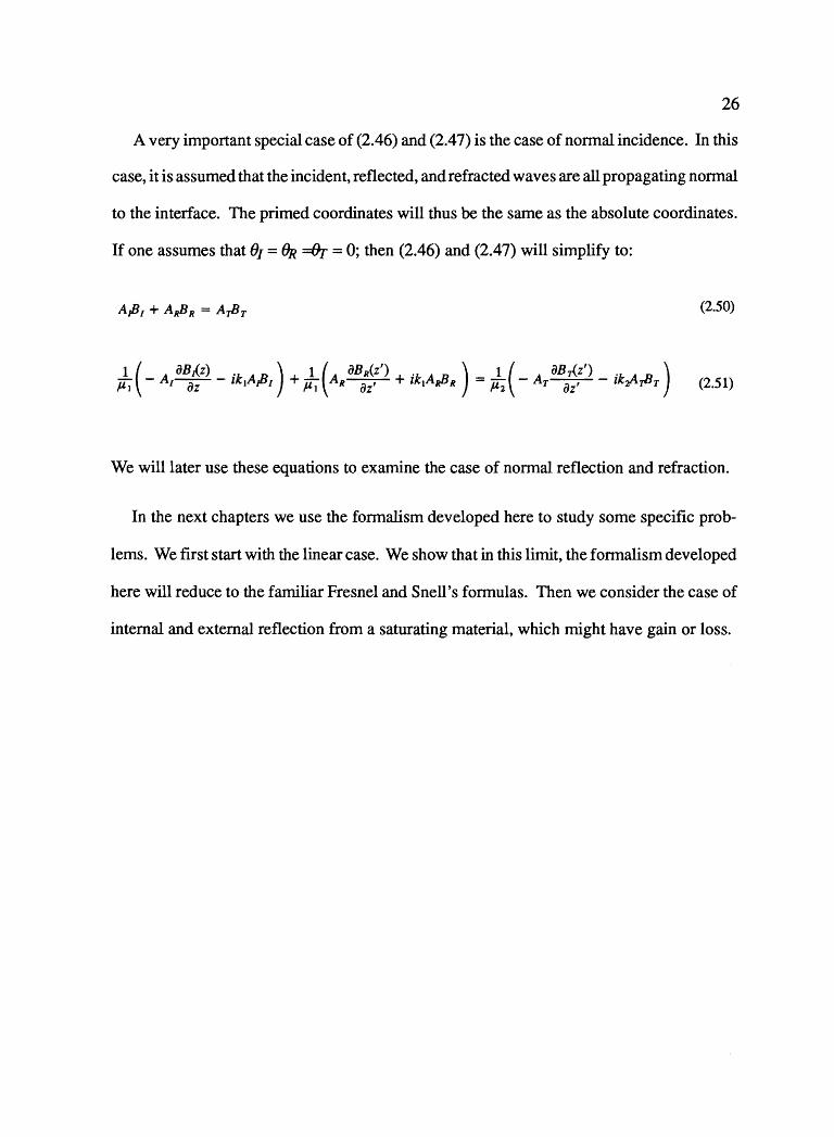
26

A very important special case of (2.46) and (2.47) is the case of normal incidence. In this

case, it is assumed that the incident, reflected, and refracted waves are all propagating normal

to the interface. The primed coordinates will thus be the same as the absolute coordinates.

If one assumes that 01 = (}R ~ = O; then (2.46) and (2.47) will simplify to:

A/11 + ARBR = A.,JJT (2.50)

1-(- A oBJ(z) - ik A 11 ) + 1-(A oBiz') + ik A 11 ) =..!..(-A oBr(z') - ik ~ 11 ) µ1 I OZ l /L'/ µ1 R oz' l JlUR µ2 T oz' 2'1'?T (2.51)

We will later use these equations to examine the case of normal reflection and refraction.

In the next chapters we use the formalism developed here to study some specific prob-

lems. We first start with the linear case. We show that in this limit, the formalism developed

here will reduce to the familiar Fresnel and Snell's formulas. Then we consider the case of

internal and external reflection from a saturating material, which might have gain or loss.

27

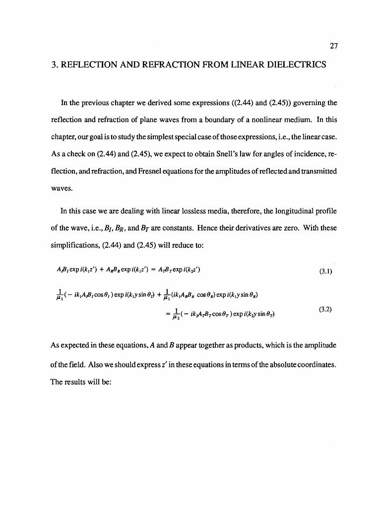
3. REFLECTION AND REFRACTION FROM LINEAR DIELECTRICS

In the previous chapter we derived some expressions ((2.44) and (2.45)) governing the

reflection and refraction of plane waves from a boundary of a nonlinear medium. In this

chapter, our goal is to study the simplest special case of those expressions, i.e., the linear case.

As a check on (2.44) and (2.45), we expect to obtain Snell's law for angles of incidence, re­

flection, and refraction, and Fresnel equations for the amplitudes of reflected and transmitted

waves.

In this case we are dealing with linear lossless media, therefore, the longitudinal profile

of the wave, i.e., B1, BR, and Br are constants. Hence their derivatives are zero. With these

simplifications, (2.44) and (2.45) will reduce to:

A/J1exp i(k1z') + A_JJR exp i(k1z') = ArBTexp i(k2z') (3.1)

J1 (- ik1A/J1cos81 )expi(k1ysin81) + J

1 (ik1Ar/JR cos8R)expi(k1ysin8R)

= J/- ik~ilJTcos8T) exp i(kiY sin8T) (3.2)

As expected in these equations, A and B appear together as products, which is the amplitude

of the field. Also we should express z' in these equations in terms of the absolute coordinates.

The results will be:

28

E1expi(k1ysin01) + ERexpi(k1ysinOR) = ETexpi(k2,}'sinOT) (3.3)

J1

( - ik1E1cos 01) exp i(k1Y sin 01) + J1 (ik1ER cos OR) exp i(k1y sin OR)

= J2

( - ik2ETcos OT) exp i(k2,}' sin OT) (3.4)

The first expression should be valid for all values of y. The only way for this to happen is

require:

exp i(k1y sin 01) = exp i(k1y sin OR) = exp i(k2,}' sin OT)

E1 +ER= ET

Expression (3.5) results in Snell's law of reflection and refraction:

k1sin01 = ki sin OR = k2 sin OT

sin01 _ k2 01 = OR ' sin OT - ki

(3.5)

(3.6)

(3.7)

Expression (3.6) relates the amplitudes of the waves, but is not conclusive by itself. We

should consider (3.4) now, which will further simplify if we use (3.7):

1 1 1 µ1 (k1E1COS01) - µ1 (k1ERcosOR) = µ2 (ki£Tcos0T) (3.8)

Combining (3.8) with (3.6) results in the familiar Fresnel formulas[l]:

29

TE = Er= 2k~2 cos01 E1 k~2 cos 01 + k'J}l1 cos Or (3.9)

RE =ER = k~2cos01 - k'lfl1 cos Or E1 k~1 cos (JI + k'J}l1 cos Or (3.10)

where TE and RE are defined as the transmission and reflection coefficients for the electric

field. Expressions (3. 9) and (3.10) are Fresnel equations for the transmission and reflection

coefficients for the case of perpendicularly polarized electric fields. Usually the materials

involved are magnetically similar, that is, µi = µ2 = µo • Also, the materials are assumed to

be pure dielectrics which means one can assumek1=mn1/c andk2=mn2/c. Substituting these

in (3.9) and (3.10), we get:

T = Er = 2n1 cos01 E - E1 n1 cos01 + n2cos0r

(3.11)

RE = ER = n1 cos01 - n2cos0r E1 n1 cos01 + n2cos0r

(3.12)

These two equations are the more familiar forms of Fresnel's equations for the reflection and

refraction of a perpendicularly polarized plane wave from the boundary of a dielectric.

It is also useful to derive the reflection and transmission coefficients for the intensity of

the waves. The transmittance of the surface is defined as the ratio of the transmitted power

to the incident power. Remembering that the power crossing a certain area is proportional

to the cosine of the angle of incidence, one can write:

2

T = Transmitted power = Ir cos 8r = n2 cos 8r (Er) = n2 cos 8r (T )2 - Incidentpower I1cosfJ1 n1cosfJ1 E1 n1cosfJ1 E

(3.13)

30

So by knowing the transmission coefficient for the electric field, one can find the transmit-

tance of the surface using (3.13).

The reflectance of an interface is defined as the ratio of the reflected power to the incident

power. So the reflectance is related to the reflection coefficient for the electric field by:

2

R = Refl~cted power = IRcosOR = IR = (ER) = (RE)2 Incident power I1cos 01 h E1 (3.14)

In chapter 4, we will generalize these formulas for the case of a nonlinear saturating medium.

We do not continue the subject of linear reflection and refraction any further as complete

discussion on this topic can be found in any standard text book[l]. Our purpose, however,

was to check the formalism developed earlier in the easiest special case and to make sure that

the reduction will result in the familiar Fresnel and Snell's formulas. Also it would be useful

to compare the expressions we derive in chapter 4 for a nonlinear interface with these stan-

dard expressions for a linear interface. In the next chapter, we study the case of a saturable

material.

~

31

4. REFLECTION AND REFRACTION AT A SATURABLE INTERFACE

4.1. LIGHT PROPAGATION IN SATURABLE AMPLIFIERS

As was discussed earlier, reflection and refraction from a nonlinear boundary is a direct

consequence of nonlinear propagation characteristics inside the materials at the two sides of

the interface. Our purpose now is to examine the case of saturable materials. These materials

might act as amplifiers, or as absorbers. The formalism for the two types is not very different.

In this study we consider the case of amplifiers.

To find the governing equation for the propagation of the light waves in a saturating am-

plifier, one might start from Maxwell's equations. Using these equations and adopting a

propagating wave form for the electric field and the polarization, one would obtain a second

order differential equation for the complex amplitude of the electric field with the polariza-

ti.on as the driving factor. For convenience, we rewrite equation (7) in ref. [2] which is the

result of the procedure just mentioned :

c2d2!~z) + 2iQcdE~z) + [w2 - Q2 + i~w jE'(z) = - 0:2 r r. P'(v,w.,z)dvdw. (4.1)

where E' ( z) is the complex amplitude of the electric field vector in x direction, c=(µe J-1/2

and !2=k(µe)-ll2, and P' is the complex amplitude of the polarization. It is also assumed

that the field is propagating in the z direction. This equation is a second order differential

equation, and it is usual to eliminate the second derivative with respect to the first derivative,

by arguing that the field envelope varies negligibly in a wave length. The resulting equation

( equation (8) in ref. [2] ) is then of first order.

32

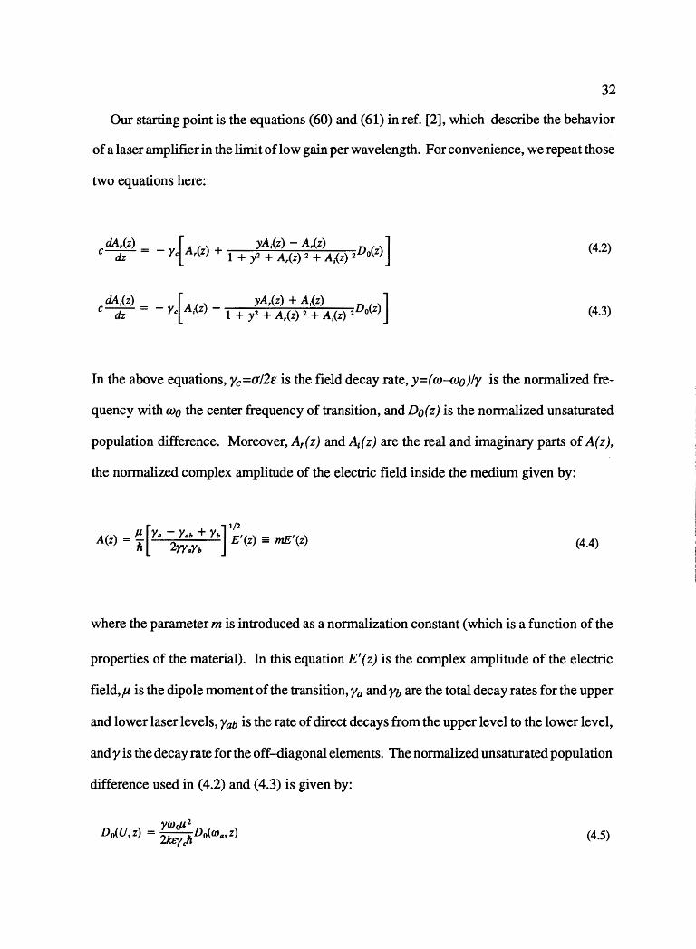
Our starting point is the equations (60) and (61) in ref. [2], which describe the behavior

of a laser amplifier in the limit oflow gain per wavelength. For convenience, we repeat those

two equations here:

dAh) [ yA;(z) - Ah) ] c~ = - Ye Ah)+ 1 + y2 +Ah) 2 + A,{z) 2Do(z) (4.2)

dA;(z) [ yAr(z) + A,{z) ] c~ = - Ye A,{z) - 1 + y2 + A,(z) 2 + A,{z) 2Do(z) (4.3)

In the above equations, Yc=a/2e is the field decay rate, y=(m--OJo)ly is the normalized fre-

quency with mo the center frequency of transition, and Do( z) is the normalized unsaturated

population difference. Moreover, A,(z) and A;(z) are the real and imaginary parts of A(z),

the normalized complex amplitude of the electric field inside the medium given by:

A(z) = /!_ Ya - Yab +Yb E'(z) = mE'(z) [ ]

1/2

Ii 2YYaYb (4.4)

where the parameter mis introduced as a normalization constant (which is a function of the

properties of the material). In this equation E'(z) is the complex amplitude of the electric

field,µ is the dipole moment of the transition, Ya and Yb are the total decay rates for the upper

and lower laser levels, Yab is the rate of direct decays from the upper level to the lower level,

and y is the decay rate for the off-diagonal elements. The normalized unsaturated population

difference used in ( 4.2) and ( 4.3) is given by:

YWcJl2 lJ0(l.J,z) = 'lkeycli[)o(Wa,z) (4.5)

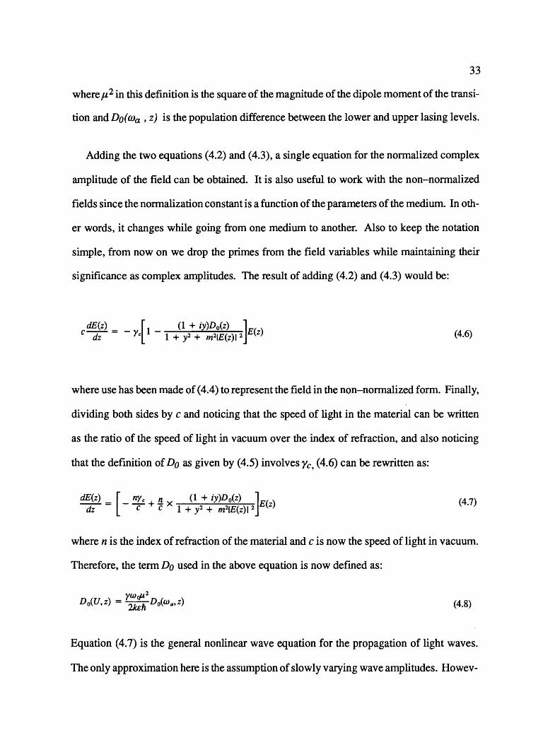
33

whereµ 2 in this definition is the square of the magnitude of the dipole moment of the transi-

ti.on andDo(ma, z) is the population difference between the lower and upper lasing levels.

Adding the two equations ( 4.2) and ( 4.3), a single equation for the normalized complex

amplitude of the field can be obtained. It is also useful to work with the non-normalized

fields since the normalization constant is a function of the parameters of the medium. In oth-

er words, it changes while going from one medium to another. Also to keep the notation

simple, from now on we drop the primes from the field variables while maintaining their

significance as complex amplitudes. The result of adding (4.2) and (4.3) would be:

dE(z) = _ [ 1 _ (1 + iy)D0(z) ]E( ) c dz Ye 1 + y2 + m21E(z}l 2 z (4.6)

where use has been made of ( 4.4) to represent the field in the non-normalized form. Finally,

dividing both sides by c and noticing that the speed of light in the material can be written

as the ratio of the speed of light in vacuum over the index of refraction, and also noticing

that the definition of Do as given by (4.5) involves Ye, (4.6) can be rewritten as:

dE(z} = [- ny c + !! X (1 + iy)D0(z) ]E(z) dz c c 1 + y2 + m21E(z}l 2

(4.7)

where n is the index of refraction of the material and c is now the speed of light in vacuum.

Therefore, the term Do used in the above equation is now defined as:

)1Wr}l2 D 0(U,z) = 2/ali D 0(w 0 ,z) (4.8)

Equation ( 4. 7) is the general nonlinear wave equation for the propagation of light waves.

The only approximation here is the assumption of slowly varying wave amplitudes. Howev-

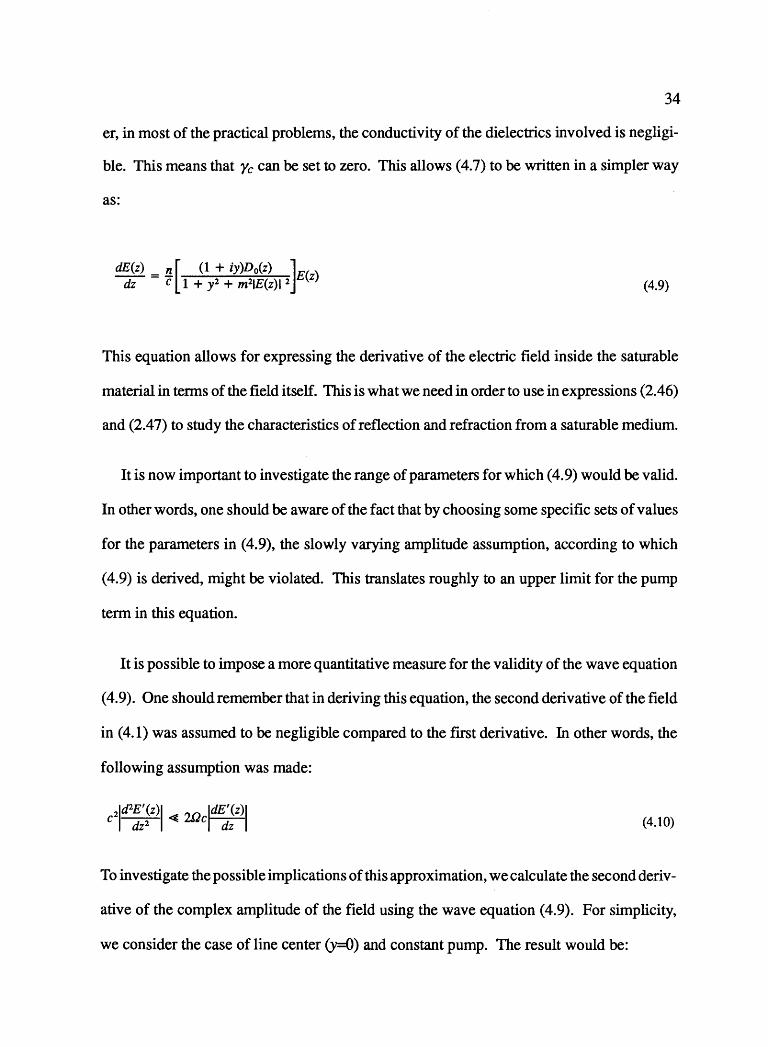
34

er, in most of the practical problems, the conductivity of the dielectrics involved is negligi-

ble. This means that Ye can be set to zero. This allows (4.7) to be written in a simpler way

as:

dE(z) = !1.[ (1 + iy)Do(z) ]E(z) dz c 1 + y2 + m21E(z)I 2 (4.9)

This equation allows for expressing the derivative of the electric field inside the saturable

material in terms of the field itself. This is what we need in order to use in expressions (2.46)

and (2.4 7) to study the characteristics of reflection and refraction from a saturable medium.

It is now important to investigate the range of parameters for which ( 4.9) would be valid.

In other words, one should be aware of the fact that by choosing some specific sets of values

for the parameters in (4.9), the slowly varying amplitude assumption, according to which

( 4.9) is derived, might be violated. This translates roughly to an upper limit for the pump

term in this equation.

It is possible to impose a more quantitative measure for the validity of the wave equation

( 4.9). One should remember that in deriving this equation, the second derivative of the field

in ( 4.1) was assumed to be negligible compared to the first derivative. In other words, the

following assumption was made:

21d2E' (z)I ,,I'"} ldE' (z)I

c dz2 ~ ~"c dz (4.10)

To investigate the possible implications of this approximation, we calculate the second deriv-

ative of the complex amplitude of the field using the wave equation ( 4.9). For simplicity,

we consider the case of line center (y=O) and constant pump. The result would be:

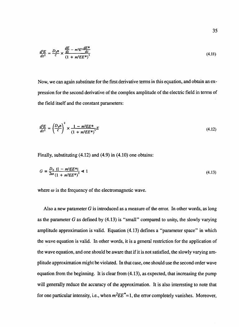
35

dE 2E2 dE* d 2E Don dz - m <iZ -=-x~---=-dz2 c (1 + m2EE*) 2

(4.11)

Now, we can again substitute for the first derivative terms in this equation, and obtain an ex-

pression for the second derivative of the complex amplitude of the electric field in terms of

the field itself and the constant parameters:

2

d2E (Don) 1 - m2EE* E dz2 = -c- X (1 + m2EE*)3

Finally, substituting (4.12) and (4.9) in (4.10) one obtains:

Do 11 - m2EE*I ~ 1 G = 2m (1 + m2EE*)2

where w is the frequency of the electromagnetic wave.

(4.12)

(4.13)

Also a new parameter G is introduced as a measure of the error. In other words, as long

as the parameter Gas defined by (4.13) is "small" compared to unity, the slowly varying

amplitude approximation is valid. Equation ( 4.13) defines a "parameter space" in which

the wave equation is valid. In other words, it is a general restriction for the application of

the wave equation, and one should be aware that if it is not satisfied, the slowly varying am-

plitude approximation might be violated. In that case, one should use the second order wave

equation from the beginning. It is clear from ( 4.13), as expected, that increasing the pump

will generally reduce the accuracy of the approximation. It is also interesting to note that

for one particular intensity, i.e., when m2EE* = 1, the error completely vanishes. Moreover,

36

in general, the condition (4.13) is better satisfied with higherintensities. This can easily be

described, since higher intensities cause a decrease in the effective gain.

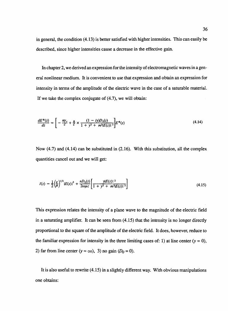
In chapter 2, we derived an expression for the intensity of electromagnetic waves in a gen-

eral nonlinear medium. It is convenient to use that expression and obtain an expression for

intensity in terms of the amplitude of the electric wave in the case of a saturable material.

If we take the complex conjugate of (4.7), we will obtain:

dE*(z) = [- ny c + !! X (1 - iy)Do(z) ]E*(z) dz c c 1 + y2 + m21E(z)l 2

(4.14)

Now (4.7) and (4.14) can be substituted in (2.16). With this substitution, all the complex

quantities cancel out and we will get:

1 (e )t/2 2 nD0(z) [ ylE(z) I 2 ] /(z) = '2 µ IE(z)I + 'lwµc 1 + y2 + m21E(z)l 2 (4.15)

This expression relates the intensity of a plane wave to the magnitude of the electric field

in a saturating amplifier. It can be seen from (4.15) that the intensity is no longer directly

proportional to the square of the amplitude of the electric field. It does, however, reduce to

the familiar expression for intensity in the three limiting cases of: 1) at line center (y = 0),

2) far from line center (y = oo ), 3) no gain (Do = 0).

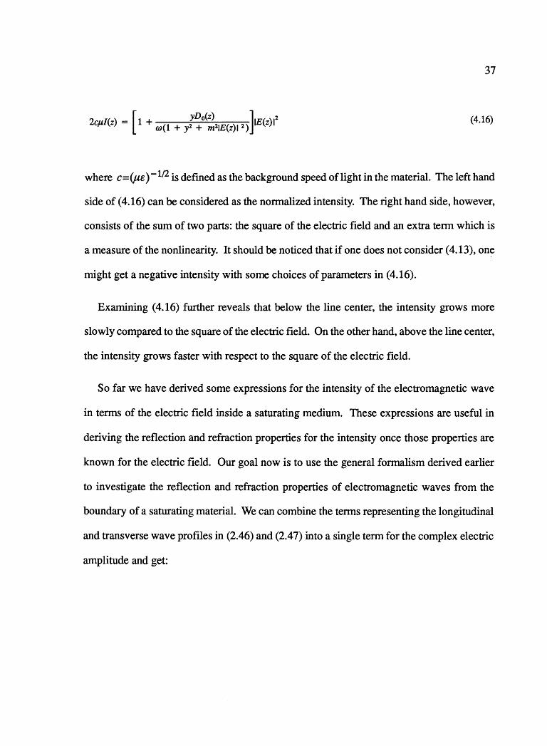
It is also useful to rewrite (4.15) in a slightly different way. With obvious manipulations

one obtains:

37

[ yDo(z) ]1E(z)l2

2cµI(z) = 1 + w(l + y2 + m21E(z)I 2 ) (4.16)

where c=(µe )-112 is defined as the background speed of light in the material. The left hand

side of ( 4.16) can be considered as the normalized intensity. The right hand side, however,

consists of the sum of two parts: the square of the electric field and an extra term which is

a measure of the nonlinearity. It should be noticed that if one does not consider ( 4.13), one

might get a negative intensity with some choices of parameters in (4.16).

Examining (4.16) further reveals that below the line center, the intensity grows more

slowly compared to the square of the electric field. On the other hand, above the line center,

the intensity grows faster with respect to the square of the electric field.

So far we have derived some expressions for the intensity of the electromagnetic wave

in terms of the electric field inside a saturating medium. These expressions are useful in

deriving the reflection and refraction properties for the intensity once those properties are

known for the electric field. Our goal now is to use the general formalism derived earlier

to investigate the reflection and refraction properties of electromagnetic waves from the

boundary of a saturating material. We can combine the terms representing the longitudinal

and transverse wave profiles in (2.46) and (2.47) into a single term for the complex electric

amplitude and get:

38

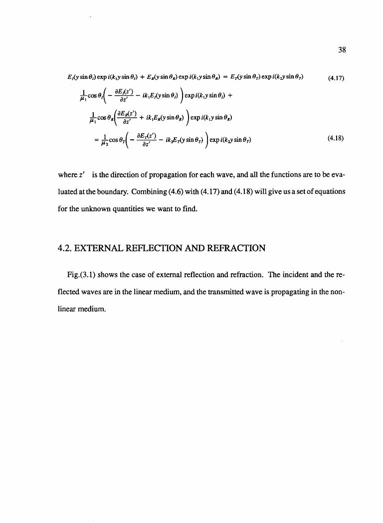
Ei(y sin81) exp i(k1y sin81) + ER(y sin BR) exp i(k1ysin8R) = E:,{y sin OT) expi(k:i.Y sin OT) (4.17)

J1 cos 61( - a~~;'> - ik1E ,(y sin 6,) ) exp i(k1y sin 6,) +

J. ros 6 .(a~~;'> + ik1E.(y sin 6 .) ) exp i(k1Y sin 6.)

= J2 cos 6,( - aEfz;'> - ik,E,{y sin 6,) ) exp i(k,y sin 6,) ( 4 .18)

where z' is the direction of propagation for each wave, and all the functions are to be eva­

luated at the boundary. Combining ( 4.6) with ( 4.17) and ( 4.18) will give us a set of equations

for the unknown quantities we want to find.

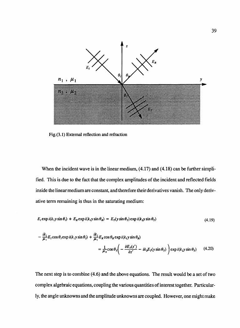
4.2. EXTERNAL REFLECTION AND REFRACTION

Fig.(3.1) shows the case of external reflection and refraction. The incident and the re­

flected waves are in the linear medium, and the transmitted wave is propagating in the non­

linear medium.

39

z

Fig.(3.1) External reflection and refraction

When the incident wave is in the linear medium, ( 4.17) and ( 4.18) can be further simpli­

fied. This is due to the fact that the complex amplitudes of the incident and reflected fields

inside the linear medium are constant, and therefore their derivatives vanish. The only deriv-

ative term remaining is thus in the saturating medium:

E1expi(k1ysin81) + ERexpi(k1ysin8R) = E:r{ysin8T)expi(k2}'sin8T) (4.19)

- ~: E1cos8,expi(k1ysin81) + ~11 ERcos8Rexpi(k1ysin8R)

= J2 cos II~ - a~~;'> - ik,E,(y sin II,) ) exp i(k,y sin II,) ( 4.20)

The next step is to combine (4.6) and the above equations. The result would be a set of two

complex algebraic equations, coupling the various quantities of interest together. Particular­

ly, the angle unknowns and the amplitude unknowns are coupled. However, one might make

40

some arguments to separate the angle and amplitude unknowns in (4.19). One, for instance,

might argue that the amplitude term in the right hand side of ( 4.19) which represents the mag­

nitude of the electric field inside the saturating medium along the boundary should be

constant because for semi-infinite plane waves there should not be any variations along the

boundary. In other words, the wave amplitudes have long reached a steady state value and

are therefore constants. With this argument, the amplitude and angle terms in (4.19) decou-

ple, and we get Snell's law of reflection and refraction, and an expression relating the ampli-

tudes of the fields:

E1 +ER= Er

81 = OR ; ki sin81 = k2 sin8r

Moreover, combining (4.9) and (4.20) will give us another expression:

(4.21)

(4.22)

;: cos IJ, (E, - E.) = ;, cos o,[ k,E, + in~. E, - i n,D/O) ( 1 + ) : ~'IE,l 2 )E,] ( 4.23)

where n2 andk2 are defined for the nonlinear medium. The two expressions ( 4.21) and ( 4.23)

can now be solved for either the reflected or transmitted amplitude in terms of the incident

amplitude. The easiest thing to do is to omit ER between (4.21) and (4.23). The result would

be:

E = (!+ µicos8r [k + .nU'c_ .n,P0(0)( 1 +iy )])E l 2 '2µ.iJc1COS81 2 l C l C l+y2+ m21E~2 T (4.24)

where n2 is the index of refraction of the nonlinear medium. Equation ( 4.24) is an algebraic

equation which relates Er and E1. So for a given angle of incidence and incident field E1,

41

( 4.24) can be solved for the transmitted field Er. Once Er is found, it can be substituted in

(4.21) to find ER. As can be seen from (4.24), to find Er in terms of E1 explicitly, one should

solve a rather difficult nonlinear complex algebraic equation. However, it is possible to treat

the saturation term in the denominator as a parameter, and obtain:

E 2µ2'c1 cos81 T=2= ]

E - E1 .nU'c .nJJo(O) 1 +iy µ,k, cos81 + µ, cos8, [ k, + •-c- - 1 c ( 1 +y'+ m'\E~ 2)

(4.25)

[ .nU'c .nPo(O) ( 1 +iy )]

E µ 2k1 cos81 - µ 1 cos8T k2 + 1-c- - z c l+y2+ m21En 2

R = _!!. = )] E - E1 .nU'c .n2Do(O) l+iy

µ,k1cos81 + µ, cos8, [ k, + 1-c- - 1 c ( 1 +y'+ m'\E~' (4.26)

where TE and RE are defined as the transmission and reflection coefficients for the electric

wave.

This representation allows us, for instance, to plot the transmission and reflection coeffi-

cients versus Er, which is related to the intensity of the incident wave. These two expres-

sions can be viewed as the generalization of the Fresnel formulas, and it is in fact easy to

check that they reduce to the Fresnel equations (3. 9) and (3.10) in the limit of no initial popu-

lation inversion (Do = 0) or in the limit of far away from the line center ( y being infinity).

The two equations ( 4.25) and ( 4.26) are a bit too complicated to use, and we can make

some simplifying assumptions to make them look simpler and easier, without loosing much

generality. In practical situations, usually the permeability of the materials involved is not

different from that of vacuum, that is: µi = µ2 = µo . Also it can be assumed that the conduc-

tivity of the materials involved is negligible. Consequently, the background propagation

42

constants of the materials ki and k2 can be assumed to be: ki = w(µoe1) 112 = wlc1 = niwlc

andk2 = w(l'<Je2) 112 = wlc2 = n2wlc. With these assumptions, (4.25) and (4.26) can be re-

written as:

E 2n1 cos01

TE = E~ = [ .D(O) ( 1 +iy )] ni cos01 + n2cos0T 1 - z-w 1 +y2+ m21En 2

(4.27)

[ .D(O) ( 1 +iy )]

ni cos01 - n2cos0T 1 - z-w 1 +y2+ m21En 2

~ ] RE = E1 = .D(O) 1 +iy n1 coslJ1 + n2cos1Jr [ 1 - •--;;;-( 1 +y2+ m2JE,j 2)

(4.28)

These equations express the external reflection and refraction coefficients for the electric

field in terms of more familiar parameters such as the indices of refraction of the two materi-

als.

It should be noticed that all these equations are based on the wave equation, which is valid

as long as the condition (4.13) is satisfied. Therefore, in using these expressions, the condi-

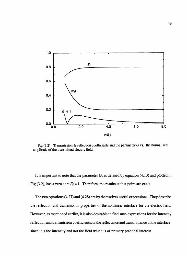
tion ( 4.13) should also be remembered. The following figure shows a typical plot of the mag-

nitude of the reflection and refraction coefficients at line center vs. the normalized magni-

tude of the transmitted electric field for a somewhat extreme choice of parameters. Also the

parameter G which was defined by ( 4.13) is plotted. As it can be seen from this figure, in-

creasing the intensity causes the transmission and reflection coefficients to approach their

saturated values, which is what Fresnel's formulas predict as well. Also, it should be noticed

that we have chosen the parameters in a way that the maximum of the parameter G is much

less than 1 (less than 0.15). The parameters used in this figure are: y=O, w =10, Do=20,

ni =l,and n2=1.5, (l/=9r=O.

1.0 ------------------~------.

0.8

0.6

0.4

0.2

0.0 0.0

G <e 1

2.0

ITEI

4.0 6.0 8.0

mlE~

Fig.(3.2) Transmission & reflection coefficients and the parameter G vs. the nonnalized amplitude of the transmitted electric field.

43

It is important to note that the parameter G, as defined by equation (4.13) and plotted in

Fig.(3.2), has a zero at mlETl=l. Therefore, the results at that point are exact.

The two equations ( 4.27) and ( 4.28) are by themselves useful expressions. They describe

the reflection and transmission properties of the nonlinear interlace for the electric field.

However, as mentioned earlier, it is also desirable to find such expressions for the intensity

reflection and transmission coefficients, or the reflectance and transmittance of the interface,

since it is the intensity and not the field which is of primary practical interest.

44

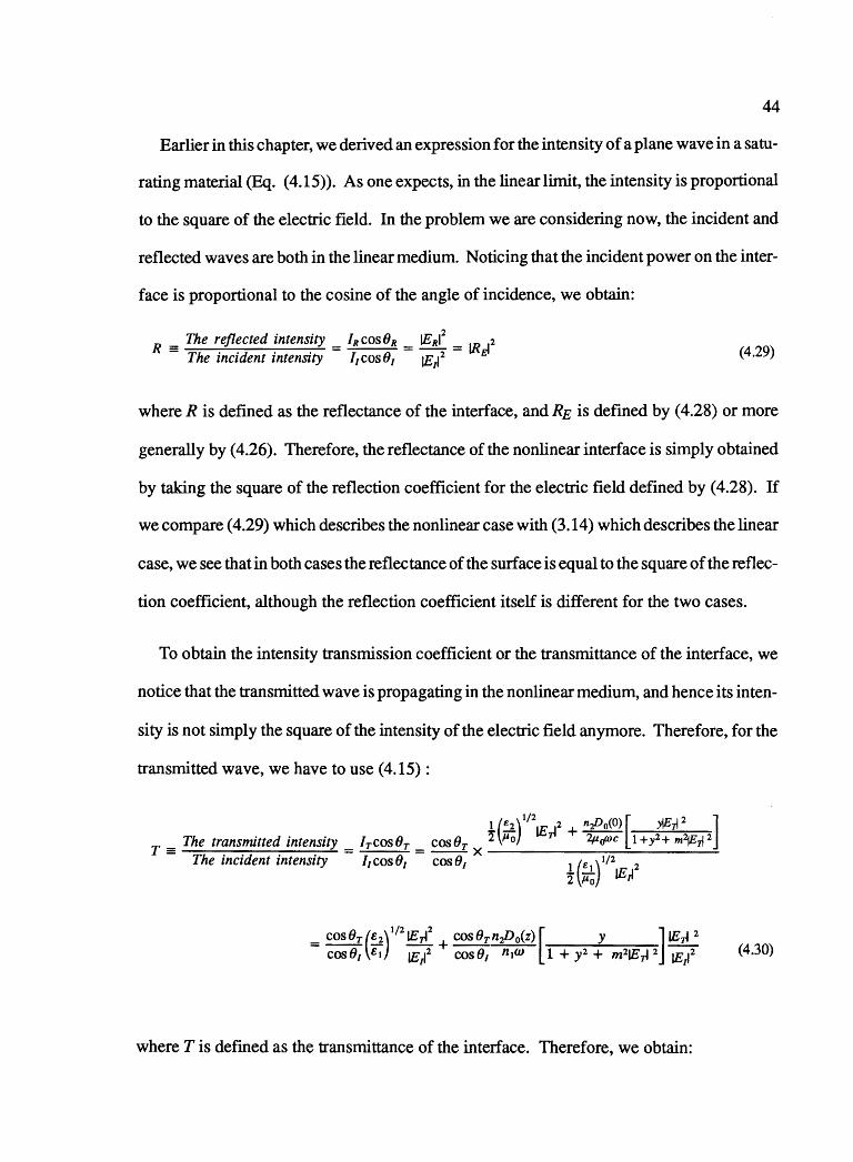
Earlier in this chapter, we derived an expression for the intensity of a plane wave in a satu-

rating material (Eq. ( 4.15) ). As one expects, in the linear limit, the intensity is proportional

to the square of the electric field. In the problem we are considering now, the incident and

reflected waves are both in the linear medium. Noticing that the incident power on the inter-

face is proportional to the cosine of the angle of incidence, we obtain:

R = The reflected intensity = IRcos(JR = IEi = IRi - The incident intensity I1cos01 IE/ (4.29)

where R is defined as the reflectance of the interface, and RE is defined by ( 4.28) or more

generally by ( 4.26). Therefore, the reflectance of the nonlinear interface is simply obtained

by taking the square of the reflection coefficient for the electric field defined by ( 4.28). If

we compare ( 4.29) which describes the nonlinear case with (3.14) which describes the linear

case, we see that in both cases the reflectance of the surface is equal to the square of the reflec-

tion coefficient, although the reflection coefficient itself is different for the two cases.

To obtain the intensity transmission coefficient or the transmittance of the interface, we

notice that the transmitted wave is propagating in the nonlinear medium, and hence its in ten-

sity is not simply the square of the intensity of the electric field anymore. Therefore, for the

transmitted wave, we have to use (4.15):

1/2 [ ] ! E2 IE 2 + n-JJ0(0) ffi'~ 2

T ,., The transmitted intensity = I ,cos 6, = cos Or x 2 ~.) :rl 2/<rfDc I+ y2 + m'IE~ 2

The incident intensity l1cos01 cos01 1 {e1)1/2 2 2 µo IEA

_ cos(JT(e 2 )112

1Ei + cos0Tn,P0(z)[ y ] IE~ 2

- cos 01 £7 IE/ cos 01 n;a> 1 + y 2 + m21E~ 2 IE/

where T is defined as the transmittance of the interface. Therefore, we obtain:

(4.30)

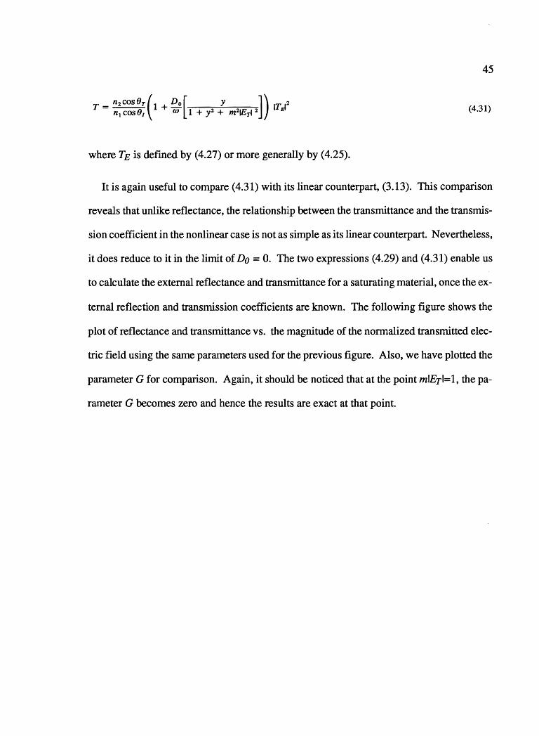
45

T _ n2 cos(JT(l +Do[ Y ]) IT 2 - n1 cosf:Jr w 1 + y2 + m21ETI 2 El (4.31)

where TE is defined by (4.27) or more generally by (4.25).

It is again useful to compare (4.31) with its linear counterpart, (3.13). This comparison

reveals that unlike reflectance, the relationship between the transmittance and the transmis-

sion coefficient in the nonlinear case is not as simple as its linear counterpart. Nevertheless,

it does reduce to it in the limit of Do = 0. The two expressions ( 4.29) and ( 4.31) enable us

to calculate the external reflectance and transmittance for a saturating material, once the ex-

ternal reflection and transmission coefficients are known. The following figure shows the

plot of reflectance and transmittance vs. the magnitude of the normalized transmitted elec-

tric field using the same parameters used for the previous figure. Also, we have plotted the

parameter G for comparison. Again, it should be noticed that at the point mlErl=l, the pa-

rameter G becomes zero and hence the results are exact at that point.

1.0 T+R

0.8

0.6

0.4

0.2

~ G

0.0 0.0 2.0 4.0 6.0

mlErl

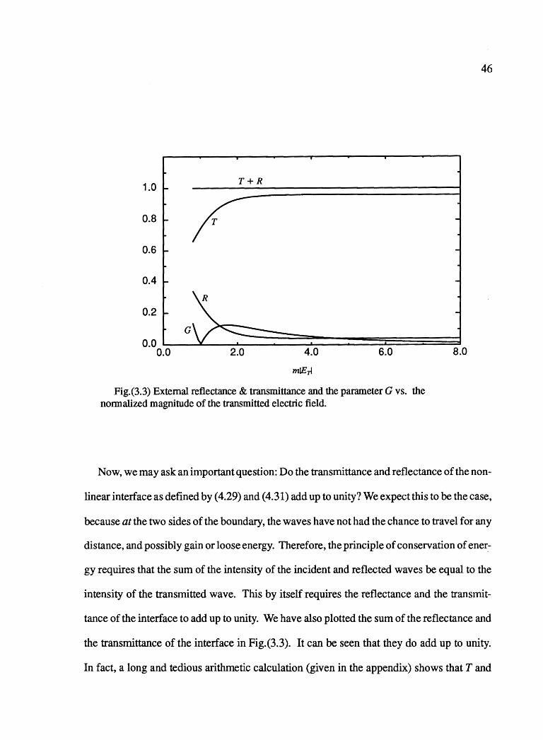
Fig.(3.3) External reflectance & transmittance and the parameter G vs. the normalized magnitude of the transmitted electric field.

46

8.0

Now, we may ask an important question: Do the transmittance and reflectance of the non-

linear interface as defined by (4.29) and (4.31) add up to unity? We expect this to be the case,

because at the two sides of the boundary, the waves have not had the chance to travel for any

distance, and possibly gain or loose energy. Therefore, the principle of conservation of ener-

gy requires that the sum of the intensity of the incident and reflected waves be equal to the

intensity of the transmitted wave. This by itself requires the reflectance and the transmit-

tance of the interface to add up to unity. We have also plotted the sum of the reflectance and

the transmittance of the interface in Fig.(3.3). It can be seen that they do add up to unity.

In fact, a long and tedious arithmetic calculation (given in the appendix) shows that T and

47

R, as defined by (4.29) and (4.31), do add up identically to unity, which is a check for them

as well.

48

5. CONCLUSION

In this study, we first developed an expression for the magnetic component of an electro­

magnetic plane wave propagating in a nonlinear material in terms of the electric component

of the wave. This expression reduced to an exact expression in the steady state case, and al­

lowed us to express the energy content or the intensity of the electromagnetic wave in terms

of the electric field component.

In chapter 2, we worked out a general frame work for the reflection and refraction of elec­

tromagnetic beams from the interface separating two nonlinear materials for arbitrary angles

of incidence. Then we discussed the special case of plane waves as beams with constant

transverse profile. It was shown that in a steady state analysis, the problem of reflection and

refraction from a nonlinear boundary can be reduced to the problem of expressing the first

derivative of the electric field amplitude at the two sides of the boundary.

Next in chapter 3, we showed that in the case of linear lossless dielectrics, the formalism

previously developed indeed reduces to the familiar Fresnel and Snell's formulas for reflec­

tion and refraction.

In chapter 4, we first discussed the propagation of light in a saturating amplifier. We fur­

ther studied the validity of the slowly varying amplitude approximation. We derived an in­

equality for the parameters which had to be satisfied if the approximation was to remain val­

id. Based on this inequality, we defined a parameter which had to be small compared to one,

if the validity of the aforementioned approximation was to be maintained.

Then we discussed the problem of external reflection and refraction from the boundary

of a saturating amplifier as a special case of the general formalism developed earlier. We

49

derived some expressions for the reflection and transmission coefficients for the electric

field component of the wave. These expressions could be considered as generalizations of

Fresnel's formulas for linear dielectrics.

Since the primary quantity of interest is usually the intensity, we also derived the same

expressions for the reflectance and transmittance of the interface using the results of the first

section. We further showed that the sum of the two is unity-consistent with the principle of

conservation of energy.

An important point in these expressions was that although the approximations for the

most part grew larger as the interface became less saturated (or equivalently, as the gain was

higher), there was one point at which they became exact: For one specific value of the trans­

mitted electric field, the parameter which we had defined as a measure of error becomes zero

and in that case, the expressions would be exact.

50

REFERENCES

[1] Hecht, "Optics", Addison-Wesley Publishing Company, second edition, 1987

[2] L. Casperson, " Field equation approximations and amplification in high-gain lasers:

Numerical results ",Physical Rev. A, Vol. 44, No. 5, Sept. 1991, p3291-3304

[3] L. Roso-Franco," Propagation of light in a nonlinear absorber", J. Opt. Soc. Am. B, Vol.

4, No. 11, Nov. 1987, p1878-1884

[ 4] A. E. Kaplan, "Theory of hysteresis reflection and refraction of light by a boundary of

a nonlinear medium", Sov. Phys. JEPT, Vol. 45, May 1977, p896-905

[5] D. Marcuse, "Reflection of a Gaussian beam from a nonlinear interface", Applied Op­

tics, Vol. 19, No. 18, Sept. 1980, p3130-3139

[6] W. Tomlinson, J. Gordon, P. Smith, A. Kaplan, "Reflection of a Gaussian beam at a non­

linear interface" Applied Optics, Vol. 21, No. 11, June 1982, p2041-2051

[7] P. Smith, W. Tomlinson, "Nonlinear Optical Interfaces: Switching Behavior", IEEE J.

Quantum Electron., Vol. QE-20, No. 1, Jan. 1984, p30-36

[8] A. Kaplan, "Conditions of Excitation of new waves (LITW) at nonlinear interface and

diagram of wave states of the system", IEEE J. Quantum Electron., Vol. QE-17, No. 3,

March 1981, p336-340

[9] P. Smith, W. Tomlinson, P. Maloney, J. Hermann, "Experimental Studies of a nonlinear

interface", IEEE J. Quantum Electron., Vol. QE-17, No. 3, March 1981, p340-348

[ 10] K. Strobl, I. Golub, " All-optical switching of reflectivity and transmissivity by a non-

51

linear sandwich", IEEE J. Quantum Electron., Vol. 28, No. 6, June 1992, p1435-1438

[11] M. Mohebi, B. Jean-Jean, J. Diels, "Self-induced reflection at a saturable interface",

Optics Lett., Vol. 14, No. 24, Dec. 1989, p1353-1355

[ 12] M. Pons, L. Roso-Franco," Reflection of a plane wave at the boundary of a saturable

absorber: Perpendicular polarization", J. Opt. Soc. Am. B, Vol. 8, No. 9, Sept. 1991,

p1876-1879

[13] L. Casperson, "Field equation approximation and the dynamics of high gain lasers",

Physical Rev. A, Vol. 43, No. 9, May 1991, p5057-5067

[14] Murry S. Spiegel, "Mathematical Handbook", Schaum's Outline Series, Mc Graw Hill,

Inc., page 59, formula 14.48

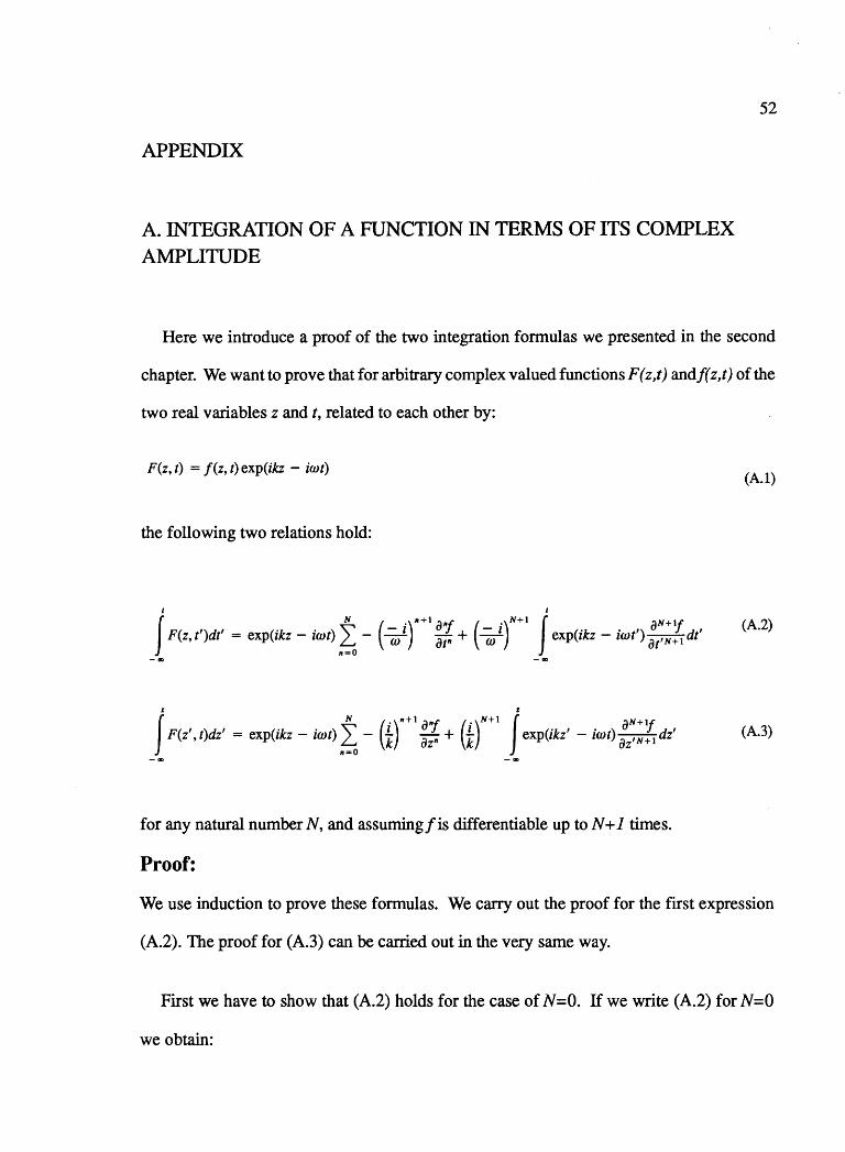
APPENDIX

A. INTEGRATION OF A FUNCTION IN TERMS OF ITS COMPLEX AMPLITUDE

52

Here we introduce a proof of the two integration formulas we presented in the second

chapter. We want to prove that for arbitrary complex valued functions F ( z,t) and/( z,t) of the

two real variables z and t, related to each other by:

F(z, t) = f (z, t) exp(ikz - iwt) (A.l)

the following two relations hold:

t t

I N (- .)"+1 o"f (- .)N+1 J 0N+1f

F(z, t')dt' = exp(ikz - iwt) ~ - w 1 ot" + w 1 exp(ikz - iwt') ot'N+t dt'

(A.2)

-~ -~

fz N (. )n+l o"f (. )N+l fz oN+1f F(z'' t)dz' = exp(ikz - iwt) I - t oz" + t exp(ikz' - iwt) oz' N + 1 dz'

,. ... o (A.3)

for any natural number N, and assuming/is differentiable up to N+l times.

Proof:

We use induction to prove these formulas. We carry out the proof for the first expression

(A.2). The proof for (A.3) can be carried out in the very same way.

First we have to show that (A.2) holds for the case of N=O. If we write (A.2) for N=O

we obtain:

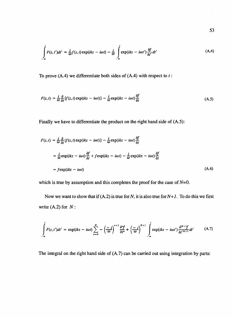
53

t t f F(z, t')dt' = !f(z, t) exp(ikz - iwt) - ! f exp(ikz - iwt') :;. dt' (A.4)

-m -m

To prove (A.4) we differentiate both sides of (A.4) with respect tot:

F(z, t) = /n :t ff (z, t) exp(ikz - iwt)] - /n exp(ikz - iwt) Z (A.5)

Finally we have to differentiate the product on the right hand side of (A.5):

F(z, t) = /n :t ff (z, t) exp(ikz - iwt)] - ~ exp(ikz - iwt) Z

= ! exp(ikz - iwt) Z + /exp(ikz - iwt) - ! exp(ikz - iwt) Z = /exp(ikz - iwt) (A.6)

which is true by assumption and this completes the proof for the case of N=O.

Now we want to show that if (A.2) is true for N, it is also true for N + 1. To do this we first

write (A.2) for N :

t t

I N (- .)11+1 o"f (- .)N+1 J aN+1f

F(z, t')dt' = exp(ikz - iwt) ~ - w l ot" + w l exp(ikz - iwt') ot'N+l dt' (A.7)

The integral on the right hand side of (A. 7) can be carried out using integration by parts:

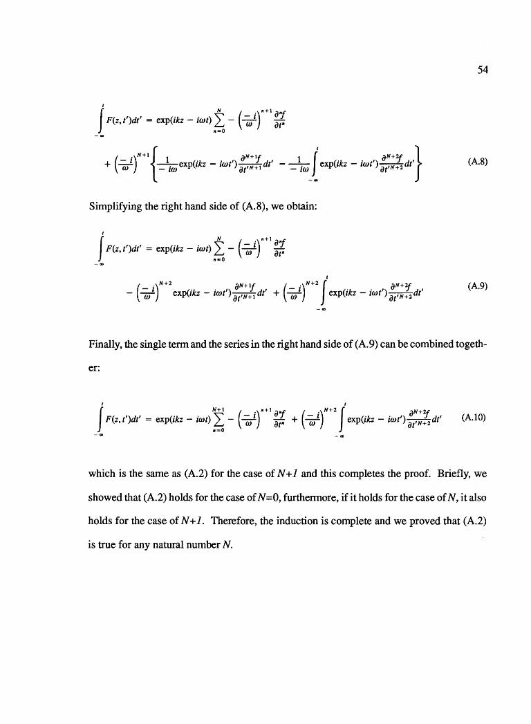
54

It N (- ,)11+1 iJ"f F(z, t')dt' = exp(ikz - iwt) b - w

1 iJtll

. N+l iJN+U iJN+U: -J 1 • • I J I 1 • • I J I

{

t } + (-;;;-) _ iw exp(zkz - zwt) at•N+• dt - _ iw_[ exp(zkz - 1wt) Ot'N+2 dt (A.8)

Simplifying the right hand side of (A.8), we obtain:

It N (- ,)11+1 iJ"f F(z, t')dt' = exp(ikz - iwt) L - w 1 iJtll

11=0

t

(- ')N+2 iJN+1f (- .)N+2 I iJN+2f (A 9)

- w 1 exp(ikz - iwt') iJt'N+l dt' + w 1

exp(ikz - iwt') iJt'N+2 dt' · ·

Finally, the single term and the series in the right hand side of (A.9) can be combined togeth-

er:

It N+l (- ')11+1 iJ"f (- ')N+2 It iJN+2f

_ • F(z, t')dt' = exp(ikz - iwt) b - ,,, 1 at• + ,,, 1 exp(ikz - iw t'} Ot' N + 2 dt' ( A.10)

which is the same as (A.2) for the case of N + 1 and this completes the proof. Briefly, we

showed that (A.2) holds for the case of N=O, furthermore, if it holds for the case of N, it also

holds for the case of N + 1. Therefore, the induction is complete and we proved that (A.2)

is true for any natural number N.

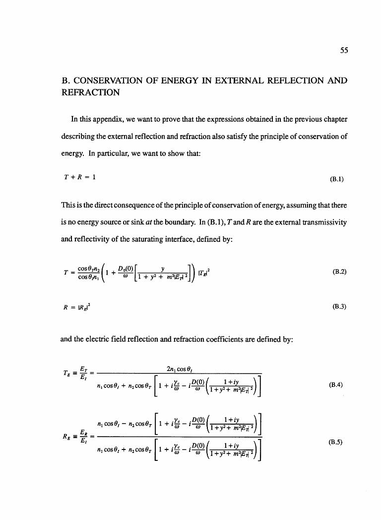
55

B. CONSERVATION OF ENERGY IN EXTERNAL REFLECTION AND REFRACTION

In this appendix, we want to prove that the expressions obtained in the previous chapter

describing the external reflection and refraction also satisfy the principle of conservation of

energy. In particular, we want to show that:

T+R = 1 (B.l)

This is the direct consequence of the principle of conservation of energy, assuming that there

is no energy source or sink at the boundary. In (B.1 ), T and R are the external transmissivity

and reflectivity of the saturating interface, defined by:

T _ cos8-in2 (i + D 0(0) [ y ]) T 2 - cos 8rn1 ---aJ 1 + y2 + m21E~ 2 I El

2 R = IREI

and the electric field reflection and refraction coefficients are defined by:

E 2n 1 cos81

TE = E~ = [ .)le .D(O) ( 1 +iy )] n1cos81 + n2cos8T 1 + 'w - 1--W- 1+y2+ m2!E~ 2

[ ·Ye .D(O) ( 1 +iy )]

E n1 cos81 - n2cos8T 1 + 'w - l(i) 1 +y2+ m2!E~ 2

R = ....!!. = )] E - E1 .Ye .D(Q) 1 +iy

n1 cos91 + n2 cos9, [ 1 + 1 m - 1w-( 1 +y•+ m2jE~ 2

(B.2)

(B.3)

(B.4)

(B.5)

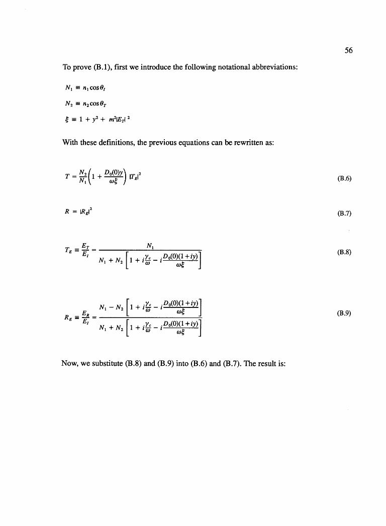
56

To prove (B.l), first we introduce the following notational abbreviations:

Ni = ni cos 81

N 2 = n2 cos8T

~ = 1 + y2 + m2IE:rf 2

With these definitions, the previous equations can be rewritten as:

T = N2 (1 + Do(O)y) ITEl2 Ni w~ (B.6)

2 R = IREI (B.7)

T, = !; = [ N1

N, + N2 1 + i~ _ iD,(0~~ +iy)] (B.8)

ER Ni - N 2 [1 + i~ _ iDo(O)(l +iy)] RE= - = w~

Er [ N1 + N2

1 + i~ _ iD,(0~~ +iy)]

(B.9)

Now, we substitute (B.8) and (B.9) into (B.6) and (B.7). The result is:

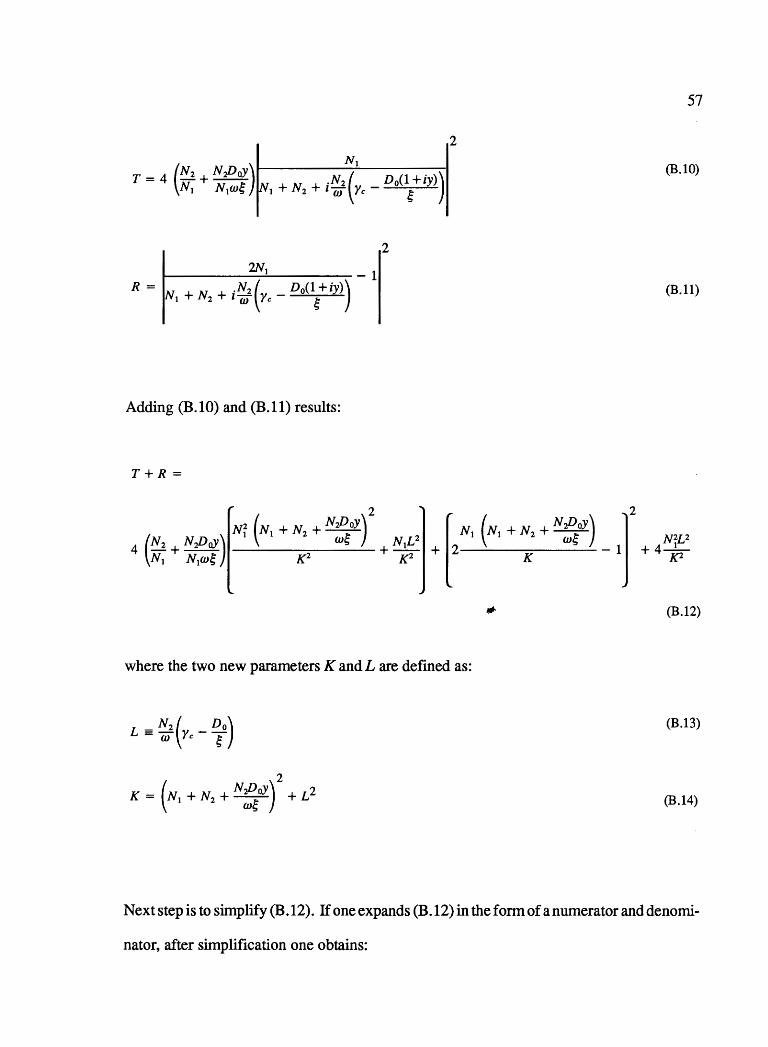
57

2

T = 4 (N2 + N PoY) Ni Niwg

Ni (B.10)

, + N 2 + i!'(r, _ Do(ltiy))

2

R= 'lNi

N( . -1 ' + N, + i w' y, - Do(lt1y)) (B.11)

Adding (B.10) and (B.11) results:

T+R =

4 (Z2 + NPoY)I~ (N, + N, + N'/:.y)2

' N,wl;, !;, N L2 K2 +-i-K2

2

[

Ni (N, + N, + N~t) l N~L2 + 2 K - 1 + 4 K2

.. (B.12)

where the two new parameters K andL are defined as:

N2 ( Do) L = w rc-T (B.13)

2

K = (N + N + NPoY) + L2 i 2 w; (B.14)

Next step is to simplify (B.12). If one expands (B.12) in the form of a numerator and denomi-

nator, after simplification one obtains:

Numerator = w 3s3(N'fw2s2 + 2N1N1fJJ 2s 2 + 2N1N,P~wy + N¥o2s 2 + 2N'f/JoYws + N'fp~2 +

+ N~~2 - 2N~ JJrl + N2,Po)

Denomi.nator = w3~3(N~w2~2 + 2N1Niro2~2 + 2N1N,Pclwy + N'~.m2~2 + 2N'¥JoYw~ + N'¥J~2 +

+ N~~2 - 2N~ JJcl + N'¥Jo)

58

The numerator and denominator are equal, and hence the right hand side of (B .12) is identi­

cally one, and the proof is complete.