Regional Development in India: Paradigms Lost in a … Geography and Economics, 2012, 53, ... Paradigms Lost in a Period of Great Change ... The number of districts changes frequently

21

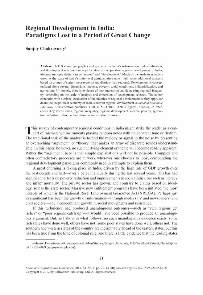
Eurasian Geography and Economics, 2012, 53, No. 1, pp. 21–43. http://dx.doi.org/10.2747/1539-7216.53.1.21Copyright © 2012 by Bellwether Publishing, Ltd. All rights reserved.

Regional Development in India: Paradigms Lost in a Period of Great Change

Sanjoy Chakravorty1

Abstract: A U.S.-based geographer and specialist in India’s urbanization, industrialization, and development outcomes surveys the state of comparative regional development in India, utilizing multiple definitions of “region” and “development.” Much of the analysis is under-taken at the scale of India’s state-level administrative units, with some additional analysis based on groups of states (meta-regions) and districts (sub-regions). Development is concep-tualized along several dimensions: income, poverty, social conditions, industrialization, and agriculture. Ultimately, there is evidence of both increasing and decreasing regional inequal-ity, depending on the scale of analysis and dimension of development selected. The author concludes with a critical evaluation of the theories of regional development as they apply (or do not) to the political economy of India’s uneven regional development. Journal of Economic Literature, Classification Numbers: I300, O150, O180, R120. 2 figures, 7 tables, 35 refer-ences. Key words: India, regional inequality, regional development, income, poverty, agricul-ture, industrialization, urbanization, administrative divisions.

This survey of contemporary regional conditions in India might strike the reader as a con-cert of mismatched instruments playing random notes with no apparent tune or rhythm.

The traditional task of the analyst is to find the melody or signal in the noise by presenting an overarching “argument” or “theory” that makes an array of disparate sounds understand-able. In this paper, however, no such unifying element or theme will become readily apparent. Rather the “argument” here is that simple explanations will not be possible. Complex and often contradictory processes are at work wherever one chooses to look, confounding the regional development paradigms commonly used in attempts to explain them.

A great churning is taking place in India, driven by the high rate of GDP growth over the past decade and half—over 7 percent annually during the last several years. This has had significant effects on poverty reduction and improvements in social indicators such as literacy and infant mortality. The private sector has grown, and contrary to claims based on ideol-ogy, so has the state sector. Massive new entitlement programs have been initiated, the most notable of which is the National Rural Employment Guarantee Act (NREGA). Perhaps just as significant has been the growth of information—through media (TV and newspapers) and civil society—and a concomitant growth in social movements and resistance.

If this turbulence had produced unambiguous outcomes—such as “rich regions get richer” or “poor regions catch up”—it would have been possible to produce an unambigu-ous argument. But, as I show in what follows, no such unambiguous evidence exists: some rich states have done well, others have not; some poor states have done well, others not. The southern and western states of the country are indisputably ahead of the eastern states, but this has been true from the time of colonial rule, and there is little evidence that the leading states

1Professor, Department of Geography and Urban Studies, Temple University, 1115 West Berks Street, Philadelphia, PA 19122-6089 ([email protected]).

22 EURASIAN GEOGRAPHY AND ECONOMICS

have forged ahead of the laggards in recent years. On the other hand, Bihar, the emblematic “basket case” of India, has been perhaps the fastest-growing state (in economic terms) over the last half decade.

Manufacturing industry may have concentrated in the leading industrial states, but it has spread from them outward to adjacent districts. At the same time, much of the job growth has been in the service sector, which is far more evenly distributed over space. Meanwhile, the agricultural sector, which still provides work for half of India’s labor force, is experiencing slow growth, most notably in the most advanced agricultural states.

A brave analyst, or an ideologically committed one, may be able to find a compelling nar-rative or argument in this. It may be possible to detect spatial patterns by looking at specific variables at specific scales. But when all the data are considered together—and for a com-prehensive view of this large and diverse country it is necessary to evaluate as much data as feasible, even in a short paper such as this one—it is intellectually indefensible to champion any particular argument. There are many spatial narratives in India today, but not a single grand story that explains everything.

My paper begins with a basic and brief description of India’s regional system and its multiple definitions. This is necessary to orient readers who are less familiar with India and to reorient those whose familiarity with the country may be limited to popular accounts: Mumbai, Bangalore, poverty, IT, slums, caste, religion, and violence. The introduction is fol-lowed by two sections. The first and longer covers the recent and current condition of regional development along several dimensions, namely income, poverty, social conditions, industri-alization, and agriculture. A second and shorter one returns to the anti-argument argument outlined above; it is an attempt to make sense of the vast variety of information presented in the first section. This final section is also where we encounter “theory,” only to dismiss (or accept) it all because, I argue, the reality of India today is too complex and fluid to be explained by any narrow theoretical or ideological approach.2

ADMINISTRATIVE AND REGIONAL SYSTEMS

Some facts about India are well known. It is a large country, more so by population than physical size. The census of 2011 counted over 1.21 billion people, a total second only to that of China (currently at about 1.33 billion), and demographers expect that by the time the 2031 census is taken, India will have overtaken China to become the world’s most populous coun-try. Between the previous census in 2001 and the current one, over 181 million people were added (Government of India, 2011). This increment alone is between the total populations of Brazil and Pakistan, the fifth- and sixth-largest countries in the world.

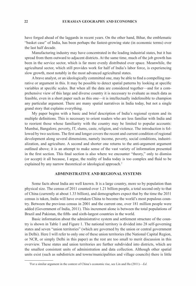
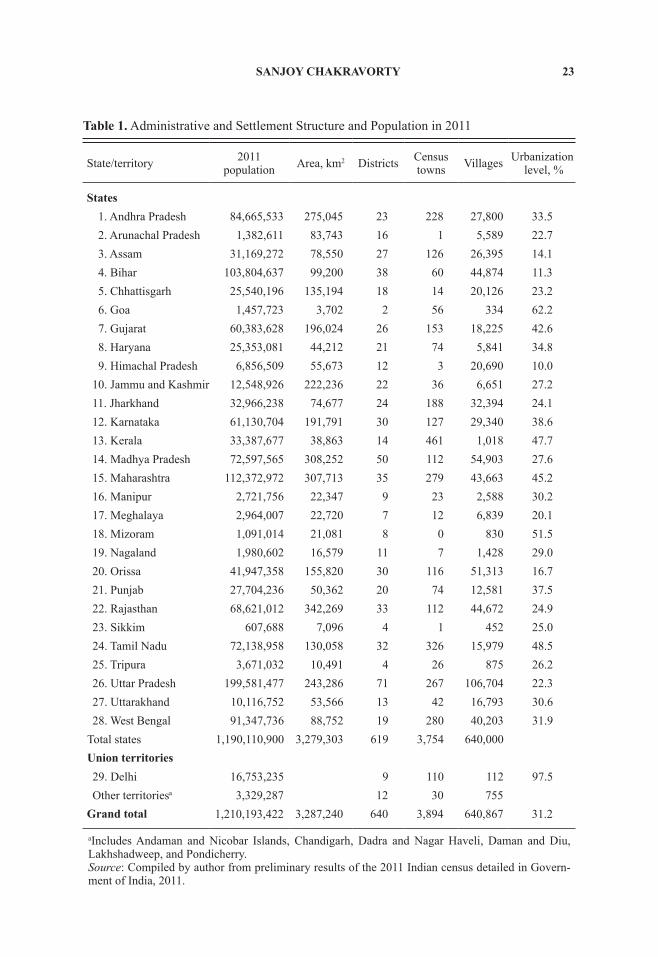
Basic information about the administrative system and settlement structure of the coun-try is shown in Table 1 and Figure 1. The national territory is divided into 28 self-governing states and seven “union territories” (which are governed by the union or central government in Delhi). Here I will refer to only one of these union territories (the National Capital Region, or NCR, or simply Delhi in this paper) as the rest are too small to merit discussion in this overview. These states and union territories are further subdivided into districts, which are the smallest consistent units of administration and data collection. Although other spatial units exist (such as subdistricts and towns/municipalities and village councils) there is little

2For a similar argument in the context of China’s economic rise, see Lin and Hu (2011)—Ed.

SANJOY CHAKRAVORTY 23

Table 1. Administrative and Settlement Structure and Population in 2011

State/territory 2011 population Area, km2 Districts Census

towns Villages Urbanization level, %

States 1. Andhra Pradesh 84,665,533 275,045 23 228 27,800 33.5 2. Arunachal Pradesh 1,382,611 83,743 16 1 5,589 22.7 3. Assam 31,169,272 78,550 27 126 26,395 14.1 4. Bihar 103,804,637 99,200 38 60 44,874 11.3 5. Chhattisgarh 25,540,196 135,194 18 14 20,126 23.2 6. Goa 1,457,723 3,702 2 56 334 62.2 7. Gujarat 60,383,628 196,024 26 153 18,225 42.6 8. Haryana 25,353,081 44,212 21 74 5,841 34.8 9. Himachal Pradesh 6,856,509 55,673 12 3 20,690 10.010. Jammu and Kashmir 12,548,926 222,236 22 36 6,651 27.211. Jharkhand 32,966,238 74,677 24 188 32,394 24.112. Karnataka 61,130,704 191,791 30 127 29,340 38.613. Kerala 33,387,677 38,863 14 461 1,018 47.714. Madhya Pradesh 72,597,565 308,252 50 112 54,903 27.615. Maharashtra 112,372,972 307,713 35 279 43,663 45.216. Manipur 2,721,756 22,347 9 23 2,588 30.217. Meghalaya 2,964,007 22,720 7 12 6,839 20.118. Mizoram 1,091,014 21,081 8 0 830 51.519. Nagaland 1,980,602 16,579 11 7 1,428 29.020. Orissa 41,947,358 155,820 30 116 51,313 16.721. Punjab 27,704,236 50,362 20 74 12,581 37.522. Rajasthan 68,621,012 342,269 33 112 44,672 24.923. Sikkim 607,688 7,096 4 1 452 25.024. Tamil Nadu 72,138,958 130,058 32 326 15,979 48.525. Tripura 3,671,032 10,491 4 26 875 26.226. Uttar Pradesh 199,581,477 243,286 71 267 106,704 22.327. Uttarakhand 10,116,752 53,566 13 42 16,793 30.628. West Bengal 91,347,736 88,752 19 280 40,203 31.9

Total states 1,190,110,900 3,279,303 619 3,754 640,000Union territories29. Delhi 16,753,235 9 110 112 97.5Other territoriesa 3,329,287 12 30 755

Grand total 1,210,193,422 3,287,240 640 3,894 640,867 31.2

aIncludes Andaman and Nicobar Islands, Chandigarh, Dadra and Nagar Haveli, Daman and Diu, Lakhshadweep, and Pondicherry. Source: Compiled by author from preliminary results of the 2011 Indian census detailed in Govern-ment of India, 2011.


consistent data available at these other scales. There are 640 districts in India, 3,894 census towns,3 and over 640,000 villages.

The states vary substantially in population size, with the largest, Uttar Pradesh, having almost 200 million people. If that state were an independent country, it would be the fifth-largest in the world; larger than Brazil, but smaller than Indonesia. The current chief minister of the state has recently argued that it should be split into four parts. Maharashtra, the second-largest state, has over 112 million people, followed by Bihar, with almost 104 million (the third state with a nine-digit population). The smallest state, Sikkim, at the other extreme, has a little over half a million people. Sikkim and the other mountainous states in the northeast

3These are to be distinguished from “statutory towns” defined during the colonial period.

Fig. 1. States and union territories of India. Parts of the northern state of Jammu and Kashmir depicted on the map are currently controlled by China and Pakistan and claimed by India.


region of the country—Arunachal Pradesh, Manipur, Meghalaya, Mizoram, and Nagaland—all have small populations (relative to India); Meghalaya at 3 million is the largest. These states will generally be ignored in much of the analysis that follows, as together they account for less than 1 percent of India’s population.

One of the difficulties in assembling consistent long-term data for India’s administrative units is that they keep changing. The number of districts changes frequently. At the time of the 2001 census there were 594 districts; by 2011 this number had grown to 640. Not only do districts change, but states do too. The last major exercise in changing state boundaries took place in 2000, when three new states were carved out of existing ones: Uttarakhand was created out of Uttar Pradesh, Jharkhand by dividing Bihar, and Chhattisgarh out of Madhya Pradesh. Therefore, Uttar Pradesh and Bihar (which are the first- and third-largest by popula-tion) and Madhya Pradesh (which is the largest by area) would have been even larger than they are presently.

Three points should be noted here. First, this review will focus on the large states because that is where 99 percent of India’s population lives. The only small state that will receive some attention is Goa, on the country’s west coast, because it is one of the leading states in terms of economic and human development. Second, many of the large states are so large that state-level averages mask significant intra-state variation. It is, therefore, appropriate to undertake sub-state or district-level analysis for such states, although this will not be pos-sible in the present brief review.4 Third, there are processes and outcomes that are discernible at scales larger than states (i.e., relevant to groups of adjacent states), and we may think of this as the meta-regional scale. It will become apparent that geographical meta-regions such as south/north/east/west do matter, as do “cultural” meta-regions such as the Hindu-Hindi heartland and the “Dravidian” south, and “developmental” regions such as “industrial” and “agricultural” states or “advanced” and “backward” ones.

Finally, a sense of how much variation may exist in development levels at the scale of states is suggested by the data on urbanization level. India is a slowly urbanizing nation. At the time of the 2001 census this level was about 28 percent and is now slightly over 31 percent. The absolute growth of the urban population outstripped that of the rural (by a few thousand people) for the first time last decade; both were about 90 million each. But despite this low level of national urbanization, there are significant state-to-state differences. Himachal Pradesh, in the foothills of the Himalayas, has reached 10 percent, Bihar is barely above 11, and Orissa is under 17 percent. On the other hand, the industrially advanced states of Maharashtra (where Mumbai is located) and Tamil Nadu (with its capital in Chennai) have crossed the 45 percent threshold. Even higher levels can be found, but they are in small and/or entirely urban states (Delhi, Goa, Mizoram).

DIMENSIONS OF STATE-LEVEL REGIONAL DEVELOPMENT

The word “development” has a rather complicated meaning. For several decades after decolonization, development was conceived in simple terms—as the growth of per capita income. But over the last three decades it has become clear that development has multiple dimensions and that its original conceptualization is best thought of as “economic develop-ment.” A region may have both relatively high levels of per capita income and poverty, which suggests that the level of inequality may be high. There is a literature on how to rank these

4In general, the analytical scale here is the state level; the small subsection presenting district-level analysis later in the paper does not do justice to the complexities at this scale.


combinations of income and inequality, but we are not interested in ranking here because grouping may be the best we can do. Also, high levels of income may coexist with relatively inferior conditions as measured by what have been called “human development” variables (e.g., life expectancy, infant mortality, literacy, nutrition, women’s empowerment, democ-racy). Sen (1985) has written extensively about “capabilities and functionings,” which, to simplify, suggests that a good society is one that allows individuals to function to the limit of their capabilities. The relevant questions to ask include: Are people free to make their own political and life decisions? Are they educated to their capacity for learning? Are they healthy? Are their children healthy? Do they live as long as their genetic inheritance allows them to? It is hence necessary to look at social or human development indicators.

Then there is the idea of “sustainable development”—that is, economic/social develop-ment that is inter-generationally transmittable by using sustainable practices (without depleting natural resources or despoiling environments). There is less clarity on the meaning of sustain-able development (Satthertwaite, 1997) and no consensus on how to measure it. Moreover, there are little data available for Indian regions that would allow us to make even first approxi-mations of sustainable development. As a result, this subject is not covered in this paper.

Income

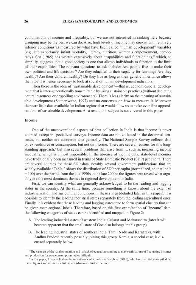
One of the unconventional aspects of data collection in India is that income is never counted except in specialized surveys. Income data are not collected in the decennial cen-suses, but neither are economic data generally. The National Sample Survey collects data on expenditures or consumption, but not on income. There are several reasons for this long-standing approach,5 but also several problems that arise from it, such as measuring income inequality, which is almost impossible. In the absence of income data, state-level incomes have traditionally been measured in terms of State Domestic Product (SDP) per capita. There are several sources for these SDP data, notably several government publications that are widely available.6 Table 2 shows the distribution of SDP per capita (normalized, so that India = 100) over the period from the late 1990s to the late 2000s; the figures here reveal what argu-ably are the most dominant themes in regional development in India.

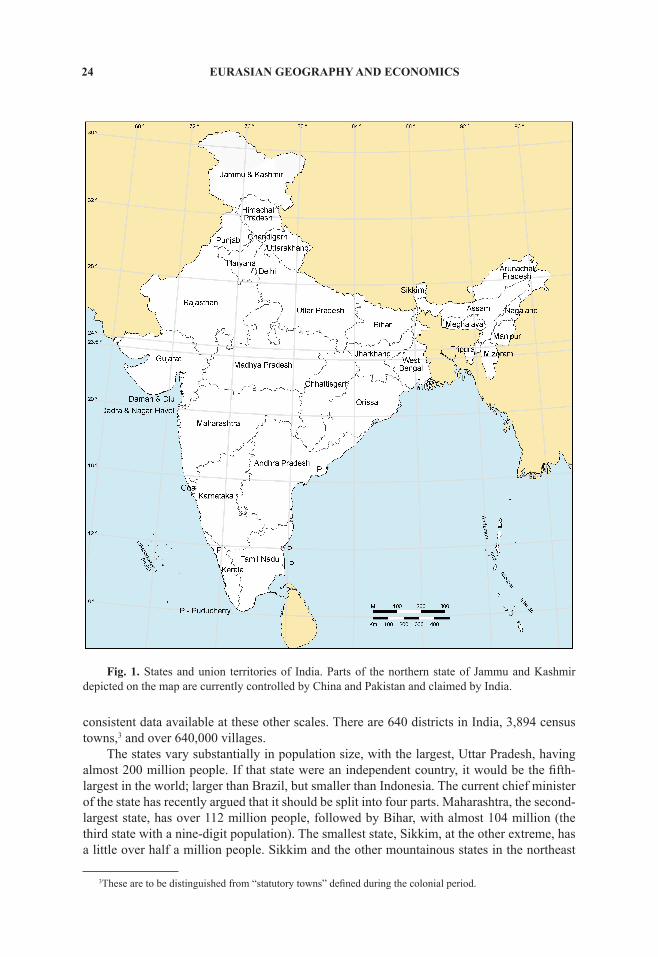
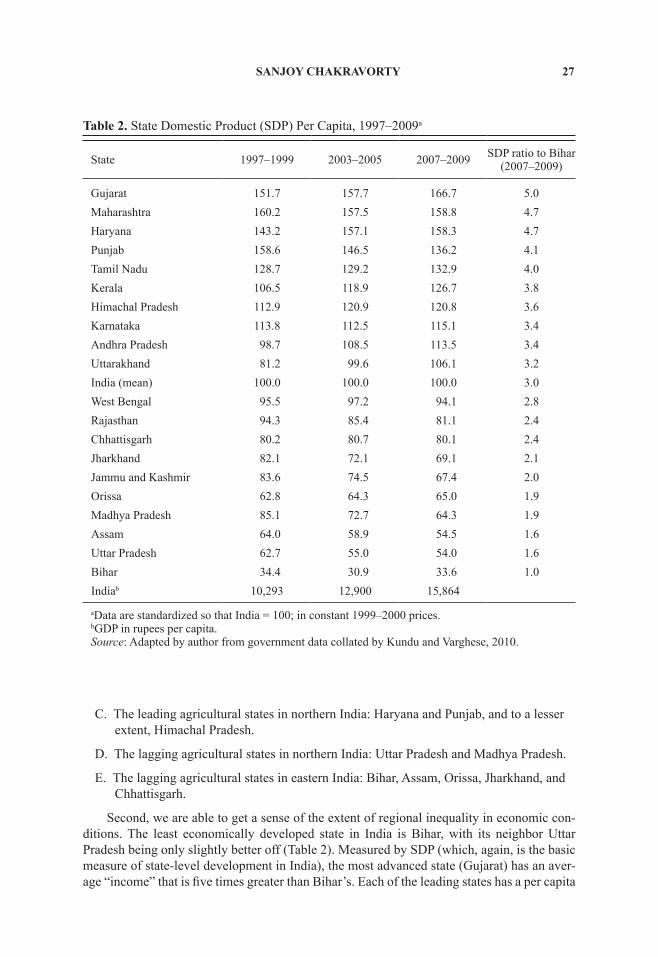
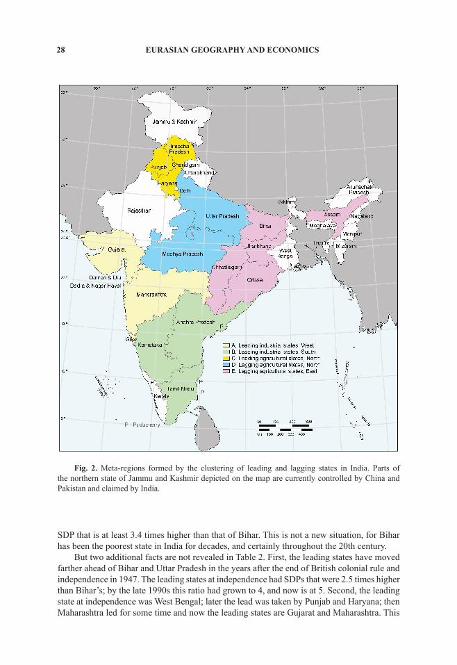
First, we can identify what are generally acknowledged to be the leading and lagging states in the country. At the same time, because something is known about the extent of industrialization and agricultural conditions in these states (detailed later in this paper), it is possible to identify the leading industrial states separately from the leading agricultural ones. Finally, it is evident that these leading and lagging states tend to form spatial clusters that can be given meta-regional labels. Therefore, based on this first examination of “income” data, the following categories of states can be identified and mapped in Figure 2:

A. The leading industrial states of western India: Gujarat and Maharashtra (later it will become apparent that the small state of Goa also belongs in this group).

B. The leading industrial states of southern India: Tamil Nadu and Karnataka, with Andhra Pradesh recently possibly joining this group. Kerala, a special case, is dis-cussed separately below.

5The vastness of the rural population and its lack of education combine to make estimations of fluctuating incomes and production for own consumption rather difficult.

6In this paper, I have relied on the recent work of Kundu and Varghese (2010), who have carefully compiled the recent figures and created useful indices (discussed further below).


C. The leading agricultural states in northern India: Haryana and Punjab, and to a lesser extent, Himachal Pradesh.

D. The lagging agricultural states in northern India: Uttar Pradesh and Madhya Pradesh.

E. The lagging agricultural states in eastern India: Bihar, Assam, Orissa, Jharkhand, and Chhattisgarh.

Second, we are able to get a sense of the extent of regional inequality in economic con-ditions. The least economically developed state in India is Bihar, with its neighbor Uttar Pradesh being only slightly better off (Table 2). Measured by SDP (which, again, is the basic measure of state-level development in India), the most advanced state (Gujarat) has an aver-age “income” that is five times greater than Bihar’s. Each of the leading states has a per capita

Table 2. State Domestic Product (SDP) Per Capita, 1997–2009a

State 1997–1999 2003–2005 2007–2009 SDP ratio to Bihar (2007–2009)

Gujarat 151.7 157.7 166.7 5.0Maharashtra 160.2 157.5 158.8 4.7Haryana 143.2 157.1 158.3 4.7Punjab 158.6 146.5 136.2 4.1Tamil Nadu 128.7 129.2 132.9 4.0Kerala 106.5 118.9 126.7 3.8Himachal Pradesh 112.9 120.9 120.8 3.6Karnataka 113.8 112.5 115.1 3.4Andhra Pradesh 98.7 108.5 113.5 3.4Uttarakhand 81.2 99.6 106.1 3.2India (mean) 100.0 100.0 100.0 3.0West Bengal 95.5 97.2 94.1 2.8Rajasthan 94.3 85.4 81.1 2.4Chhattisgarh 80.2 80.7 80.1 2.4Jharkhand 82.1 72.1 69.1 2.1Jammu and Kashmir 83.6 74.5 67.4 2.0Orissa 62.8 64.3 65.0 1.9Madhya Pradesh 85.1 72.7 64.3 1.9Assam 64.0 58.9 54.5 1.6Uttar Pradesh 62.7 55.0 54.0 1.6Bihar 34.4 30.9 33.6 1.0Indiab 10,293 12,900 15,864

aData are standardized so that India = 100; in constant 1999–2000 prices.bGDP in rupees per capita.Source: Adapted by author from government data collated by Kundu and Varghese, 2010.


SDP that is at least 3.4 times higher than that of Bihar. This is not a new situation, for Bihar has been the poorest state in India for decades, and certainly throughout the 20th century.

But two additional facts are not revealed in Table 2. First, the leading states have moved farther ahead of Bihar and Uttar Pradesh in the years after the end of British colonial rule and independence in 1947. The leading states at independence had SDPs that were 2.5 times higher than Bihar’s; by the late 1990s this ratio had grown to 4, and now is at 5. Second, the leading state at independence was West Bengal; later the lead was taken by Punjab and Haryana; then Maharashtra led for some time and now the leading states are Gujarat and Maharashtra. This

Fig. 2. Meta-regions formed by the clustering of leading and lagging states in India. Parts of the northern state of Jammu and Kashmir depicted on the map are currently controlled by China and Pakistan and claimed by India.


Table 3. Average Annual Growth of State Domestic Product, by Plan Period (ranked)

StateEighth Plan

(1992–1997)

StateNinth Plan

(1997–2002)

StateTenth Plan

(2002–2007)

Gujarat 12.4 Sikkim 8.3 Manipur 11.6Goa 8.9 Tripura 7.4 Jharkhand 11.1Maharashtra 8.9 Karnataka 7.2 Gujarat 10.6Nagaland 8.9 West Bengal 6.9 Chhattisgarh 9.2Rajasthan 7.3 Manipur 6.4 Orissa 9.1Tamil Nadu 7.0 Tamil Nadu 6.3 Uttarakhand 8.8Tripura 6.6 Meghalaya 6.2 Tripura 8.7Himachal Pradesh 6.5 Himachal Pradesh 5.9 Nagaland 8.3Kerala 6.5 Kerala 5.7 Maharashtra 7.9Madhya Pradesh 6.3 Goa 5.5 Goa 7.8West Bengal 6.3 Jammu & Kashmir 5.2 Sikkim 7.7Karnataka 6.2 Orissa 5.1 Haryana 7.6Andhra Pradesh 5.4 Maharashtra 4.7 Himachal Pradesh 7.3Sikkim 5.3 Andhra Pradesh 4.6 Kerala 7.2Haryana 5.2 Arunachal Pradesh 4.4 Karnataka 7.0Arunachal Pradesh 5.1 Punjab 4.4 Andhra Pradesh 6.7Jammu and Kashmir 5.0 Haryana 4.1 Tamil Nadu 6.6Uttar Pradesh 4.9 Bihar 4.0 Assam 6.1Punjab 4.7 Gujarat 4.0 West Bengal 6.1Manipur 4.6 Madhya Pradesh 4.0 Mizoram 5.9Meghalaya 3.8 Uttar Pradesh 4.0 Arun. Pradesh 5.8Assam 2.8 Rajasthan 3.5 Meghalaya 5.6Bihar 2.2 Nagaland 2.6 Jammu & Kashmir 5.2Orissa 2.1 Assam 2.1 Rajasthan 5.0Chhattisgarh n.a. Chhattisgarh n.a. Bihar 4.7Jharkhand n.a. Jharkhand n.a. Uttar Pradesh 4.6Mizoram n.a. Mizoram n.a. Punjab 4.5Uttarakhand n.a. Uttarakhand n.a. Madhya Pradesh 4.3India 6.5 India 5.5 India 7.7

Summary growth ratesMore developed states 7.2 5.2 7.0Special Category states 5.7 5.8 7.3Less developed states 3.7 3.8 7.2CV in growth rates 38.8 29.9 27.8

an.a. = not available; CV = coefficient of variation. The leading (more developed) states are Gujarat, Maharashtra, Haryana, Punjab, Tamil Nadu, and Karnataka. The lagging (less developed) states are Assam, Bihar, Orissa, Jharkhand, Chhattisgarh, Madhya Pradesh, Uttar Pradesh, and Uttarakhand. The Special Category states (as identified by the government of India) are Arunachal Pradesh, Assam, Manipur, Meghalaya, Mizoram, Nagaland, Jammu and Kashmir, Himachal Pradesh, and Uttarakhand.. Note that these are not mutually exclusive categories, nor do the three categories together account for all of India’s states.Source: Adapted by author from government data collated by Kundu and Varghese, 2010.


suggests that the leading edge of the economy has shifted from agriculture-based to manufac-turing-based activities.7 I will return to this idea in the paper’s concluding section.

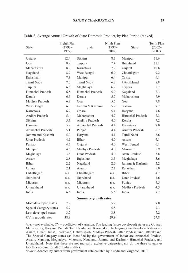
If these figures suggest a familiar narrative—rich regions get richer—the data in Table 3 give cause for pause. Here we can examine average annual rates of growth in SDP by plan period over the last three completed plans.8 The Eighth Plan (1992–1997), the first period for which data are presented here, began the year after what is widely considered to be the point of departure for the political economy of modern India—the start of economic reforms that began to move India from a command-and-control state economy to a more lib-eral, market-oriented economy with fewer restrictions on activities and decisions. Among the restrictions that were relaxed were investment location decisions of private firms, including multinationals.9

In those first years after liberalization, the narrative of “rich get richer” seemed to be obviously true. The leading states, especially the industrial states of Gujarat, Maharashtra, and Goa (all in the west), had the fastest-growing economies, and the lagging agricultural states in the east (Orissa, Bihar, and Assam) experienced the slowest growth. The more devel-oped states had growth rates almost twice as high as the less developed ones. The average annual growth rate in Gujarat was almost six times higher than the growth rates in Orissa and Bihar; in Maharashtra it was about four times higher.

But by the time the Ninth Plan (1997–2002) had concluded, the simple narrative had become more complicated. The “more developed states” as a group grew faster than the “less developed states” as a group, but the growth of both groups was less than that of India as a whole. This means that a middle category of states—neither more nor less developed in this categorical system—which included states like West Bengal and Kerala, grew faster; and the small, special category states of the northeast grew fastest. Gujarat, the undisputed leader of the Eighth Plan, grew by 4 percent, only one-third of its earlier annual rate, and considerably below the national average. In fact, it recorded the fourth-lowest rate of the states listed in the table. Maharashtra’s growth, at 4.7 per cent, was almost halved. Punjab and Haryana, the leading agricultural states, grew even more slowly than that.

The Tenth Plan (2002–2007) yielded additional surprises. Among the growth leaders were Jharkhand (over 11 percent per year), Chhattisgarh, and Orissa (both over 9 percent)—three of the least-developed states in the country. Gujarat rebounded (average annual growth of >10 percent) and Maharashtra did well (at almost 8 per cent), but Punjab, at 4.5 percent, emerged as the second-slowest growing state.

A note on Bihar is warranted. Although its growth through the Tenth Plan period was low (4.7 percent annually), data released more recently show that by the end of the Tenth Plan, under a new government with new leadership, Bihar had started to grow rapidly. It is now estimated that between 2004–2005 and 2008–2009 Bihar’s economy grew at >11 per-cent annually and in 2010–2011 by >14 percent (Bihar, 2011). There is much discussion in the media about “India’s new miracle economy” and whether these growth rates are real and sustainable. This debate is all the more relevant because recent media reports suggest that the best growth performers in the Eleventh Plan period have been the eastern lagging states of Bihar, Chhattisgarh, and West Bengal, whereas the established leaders like Gujarat and Maharashtra are no better than middle-of-the pack performers (Mayawati, 2011).

7For details see Chakravorty (2000), Chakravorty and Lall (2007), and Singh et al. (n.d.).8India follows a system of five-year plans inspired by the Soviet Union, a system that continues, perhaps more

stronger than ever, despite the demise of the inspiration.9There are many reviews of this significant structural shift, many of them ideological. Dehejia (1993) represents

an early version.


Poverty and Social Development

State-level data on poverty and social development are presented in Tables 4 and 5, respectively. Poverty is addressed first, as it is an important and widely discussed phenom-enon in India. One of the main points of discussion is the meaning and measurement of pov-erty. There are several ways of giving measurable meaning to poverty; the two more common methods use either the income equivalent of a minimum “calorie intake” (ranging from 1,800 to 2,500 calories per day) or the income equivalent of a “basket of goods” (that includes food, housing, clothing, energy, and other basic needs). Measurement has its own pitfalls and chal-lenges, including issues relating to family size, spatial adjustment of cost of living indices, and the specific thresholds to use to identify individuals below the poverty line. In India, there are also questions about the quality of the data used to identify and count the poor, because the methods used by the data gathering agency, the National Sample Survey Organization, may be outdated. For the purposes of this paper, it is not necessary to delve into the details, which tend to be more relevant to policymaking than an intellectual understanding of poverty. Here I use what is considered a standard measure (used by India’s Planning Commission) that in a sense is the country’s “official” rate. It is worth noting, however, that this poverty line is low by international standards,10 which means that it is relatively easier for Indians to be counted as non-poor while at the same time having a living standard that is indistinguishable from that of being poor.

The most recent and exhaustive analysis of poverty in India is a World Bank (2011) report (carefully and methodically prepared, it should be of great interest to researchers). The present paper utilizes poverty data collected by the Government of India, because the World Bank report does not present comprehensive data on regional poverty differences at the state level. As a test of the comparability of Indian Government and World Bank data, Table 4 pres-ents results for 2004–2005 (the most recent period analyzed in the World Bank report). The two sources are very close when areas of coverage overlap, such as for urban poverty rates by state (presented as Table 2.2 in World Bank, 2011, p. 84).

The salient trends in Indian poverty are summarized in the World Bank (2011) report:

(a) India has continued to record steady progress in reducing consumption poverty. (p. 4)

In 1983, rural and urban poverty rates were 47 and 42 percent respectively; these had fallen to 28 and 26 percent in 2004–2005. But because of the tremendous growth in population over the same period, the absolute number of poor has not declined appreciably and remains around 300 million.

(b) Growth has tended to reduce poverty. But problems with data cloud our assessment of whether the growth process has become more or less pro-poor in the postreform period. (pp. 6–7)

This is a contentious subject in India—whether the 1991 reforms are pro-capitalist, neolib-eral, pro-poor, anti-state, etc.—and infused with rhetoric and emotion. I return to this issue in the concluding section of the paper.

(c) Large differences in poverty levels persist across India’s states and indeed are growing in urban areas … [and] rural areas of India’s poorest states have poverty rates that are comparable to the highest anywhere in the developing world. (p. 8)

10It represents the Purchasing Power Parity (PPP) equivalent of approximately US$1.30 per person per day, com-pared to the more common international rate of $2 per person per day.


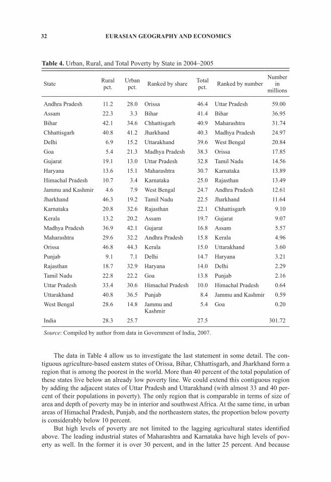
The data in Table 4 allow us to investigate the last statement in some detail. The con-tiguous agriculture-based eastern states of Orissa, Bihar, Chhattisgarh, and Jharkhand form a region that is among the poorest in the world. More than 40 percent of the total population of these states live below an already low poverty line. We could extend this contiguous region by adding the adjacent states of Uttar Pradesh and Uttarakhand (with almost 33 and 40 per-cent of their populations in poverty). The only region that is comparable in terms of size of area and depth of poverty may be in interior and southwest Africa. At the same time, in urban areas of Himachal Pradesh, Punjab, and the northeastern states, the proportion below poverty is considerably below 10 percent.

But high levels of poverty are not limited to the lagging agricultural states identified above. The leading industrial states of Maharashtra and Karnataka have high levels of pov-erty as well. In the former it is over 30 percent, and in the latter 25 percent. And because

Table 4. Urban, Rural, and Total Poverty by State in 2004–2005

State Rural pct.

Urban pct. Ranked by share Total

pct. Ranked by numberNumber

in millions

Andhra Pradesh 11.2 28.0 Orissa 46.4 Uttar Pradesh 59.00Assam 22.3 3.3 Bihar 41.4 Bihar 36.95Bihar 42.1 34.6 Chhattisgarh 40.9 Maharashtra 31.74Chhattisgarh 40.8 41.2 Jharkhand 40.3 Madhya Pradesh 24.97Delhi 6.9 15.2 Uttarakhand 39.6 West Bengal 20.84Goa 5.4 21.3 Madhya Pradesh 38.3 Orissa 17.85Gujarat 19.1 13.0 Uttar Pradesh 32.8 Tamil Nadu 14.56Haryana 13.6 15.1 Maharashtra 30.7 Karnataka 13.89Himachal Pradesh 10.7 3.4 Karnataka 25.0 Rajasthan 13.49Jammu and Kashmir 4.6 7.9 West Bengal 24.7 Andhra Pradesh 12.61Jharkhand 46.3 19.2 Tamil Nadu 22.5 Jharkhand 11.64Karnataka 20.8 32.6 Rajasthan 22.1 Chhattisgarh 9.10Kerala 13.2 20.2 Assam 19.7 Gujarat 9.07Madhya Pradesh 36.9 42.1 Gujarat 16.8 Assam 5.57Maharashtra 29.6 32.2 Andhra Pradesh 15.8 Kerala 4.96Orissa 46.8 44.3 Kerala 15.0 Uttarakhand 3.60Punjab 9.1 7.1 Delhi 14.7 Haryana 3.21Rajasthan 18.7 32.9 Haryana 14.0 Delhi 2.29Tamil Nadu 22.8 22.2 Goa 13.8 Punjab 2.16Uttar Pradesh 33.4 30.6 Himachal Pradesh 10.0 Himachal Pradesh 0.64Uttarakhand 40.8 36.5 Punjab 8.4 Jammu and Kashmir 0.59West Bengal 28.6 14.8 Jammu and

Kashmir 5.4 Goa 0.20

India 28.3 25.7 27.5 301.72

Source: Compiled by author from data in Government of India, 2007.


Maharashtra is a large state (second in both area and population), the absolute number of poor is also high—almost 32 million. This is less than the very large numbers in Uttar Pradesh (59 million) and Bihar (37 million), but a very significant number indeed (Government of India, 2007).

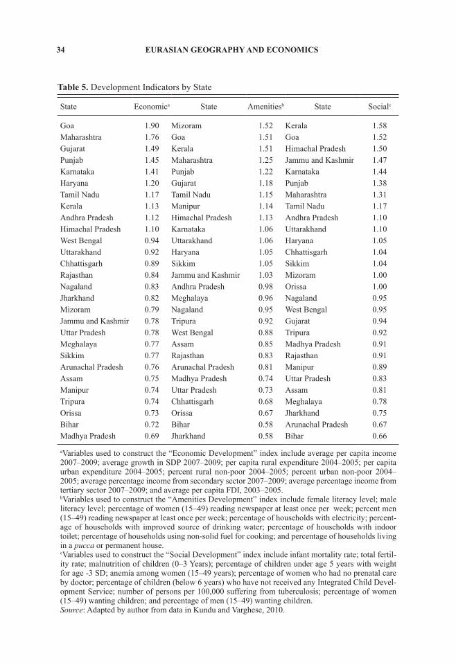
This seeming contradiction—between the label “leading industrial state” (used justifi-ably for Maharashtra) and its high level of poverty—is brought to the fore when one examines the three indicators of development presented in Table 5. The indicators “economic,” “ameni-ties,” and “social” are composite indices created by the combination of several variables (see the notes in Table 5); like all composite indices their values will fluctuate depending on the variables selected and the weights assigned to them. It is hence possible to quibble with these indexes, perhaps dispute some of the rankings, but heuristically they make sense to me. The general orders and magnitudes seem about right.

Rankings on the economic index indicate what we have come to expect at this point. The large states identified as leading states from Table 2 also constitute the upper tier of this list, topped by Goa (a small state), followed by Maharashtra. Gujarat, Punjab, and Karnataka form a cluster some distance behind the two leaders, but some distance ahead of the next cluster consisting of Haryana, Tamil Nadu, Kerala, Andhra Pradesh, and Himachal Pradesh. Madhya Pradesh, Bihar, and Orissa are at the bottom; the only surprise is that Bihar is not last. The upper tier of the amenities index exhibits a significant degree of overlap with the economic index; more or less the same states show up in the top tier, although not ranked quite as high as before because Mizoram (a very small state) and Kerala have moved up. The expected states comprise the bottom tier: Jharkhand, Bihar, Orissa, Chhattisgarh, Uttar Pradesh, and Madhya Pradesh.

The social index, however, reveals a significantly different picture. If the amenities index is constructed by use of education and housing variables, the social index broadly consists of health variables. Kerala and Goa top this list, followed by Himachal Pradesh and Jammu and Kashmir. Several leaders from the other lists rank much lower here. Maharashtra is seventh and Haryana eleventh. Gujarat ranks 18th and has a score that is lower than the national aver-age and even below Chhattisgarh and Orissa. The bottom of the list includes some expected members (Bihar, Jharkhand, Uttar Pradesh) and states from the northeast (Arunachal Pradesh, Meghalaya, Assam). Media reporting on the Human Development Report 2011 indicate simi-lar rankings—Kerala, Delhi, Himachal Pradesh, and Goa on top, followed by Punjab, the northeast, Maharashtra, Tamil Nadu, and Haryana, with Gujarat further below. This much is clear: a high level of economic development does not necessarily lead to a high level of human or social development in India.

By now it is also clear that Goa is a special state. It is small but highly developed (by Indian standards) on all economic and human development scales. Kerala too is special; although its economy is not as developed as its neighbors in southern or western India, the quality of life is excellent. Kerala’s virtues are well known in India. It was the first state to achieve 100 percent literacy, first to lower its fertility rate to the replacement level, and is the only large state to have more women than men.11 Kerala has also been run by communist parties, off and on, for the last several decades.12

11Without female foeticide, this would be the case throughout the country.12Before one gets carried away with the social virtues of communist parties of India, it is useful to note that the

two other states with long-term communist administrations—West Bengal and Tripura—rank below the national average and in the bottom half or third in all the indices.


Table 5. Development Indicators by State

State Economica State Amenitiesb State Socialc

Goa 1.90 Mizoram 1.52 Kerala 1.58Maharashtra 1.76 Goa 1.51 Goa 1.52Gujarat 1.49 Kerala 1.51 Himachal Pradesh 1.50Punjab 1.45 Maharashtra 1.25 Jammu and Kashmir 1.47Karnataka 1.41 Punjab 1.22 Karnataka 1.44Haryana 1.20 Gujarat 1.18 Punjab 1.38Tamil Nadu 1.17 Tamil Nadu 1.15 Maharashtra 1.31Kerala 1.13 Manipur 1.14 Tamil Nadu 1.17Andhra Pradesh 1.12 Himachal Pradesh 1.13 Andhra Pradesh 1.10Himachal Pradesh 1.10 Karnataka 1.06 Uttarakhand 1.10West Bengal 0.94 Uttarakhand 1.06 Haryana 1.05Uttarakhand 0.92 Haryana 1.05 Chhattisgarh 1.04Chhattisgarh 0.89 Sikkim 1.05 Sikkim 1.04Rajasthan 0.84 Jammu and Kashmir 1.03 Mizoram 1.00Nagaland 0.83 Andhra Pradesh 0.98 Orissa 1.00Jharkhand 0.82 Meghalaya 0.96 Nagaland 0.95Mizoram 0.79 Nagaland 0.95 West Bengal 0.95Jammu and Kashmir 0.78 Tripura 0.92 Gujarat 0.94Uttar Pradesh 0.78 West Bengal 0.88 Tripura 0.92Meghalaya 0.77 Assam 0.85 Madhya Pradesh 0.91Sikkim 0.77 Rajasthan 0.83 Rajasthan 0.91Arunachal Pradesh 0.76 Arunachal Pradesh 0.81 Manipur 0.89Assam 0.75 Madhya Pradesh 0.74 Uttar Pradesh 0.83Manipur 0.74 Uttar Pradesh 0.73 Assam 0.81Tripura 0.74 Chhattisgarh 0.68 Meghalaya 0.78Orissa 0.73 Orissa 0.67 Jharkhand 0.75Bihar 0.72 Bihar 0.58 Arunachal Pradesh 0.67Madhya Pradesh 0.69 Jharkhand 0.58 Bihar 0.66

aVariables used to construct the “Economic Development” index include average per capita income 2007–2009; average growth in SDP 2007–2009; per capita rural expenditure 2004–2005; per capita urban expenditure 2004–2005; percent rural non-poor 2004–2005; percent urban non-poor 2004–2005; average percentage income from secondary sector 2007–2009; average percentage income from tertiary sector 2007–2009; and average per capita FDI, 2003–2005.bVariables used to construct the “Amenities Development” index include female literacy level; male literacy level; percentage of women (15–49) reading newspaper at least once per week; percent men (15–49) reading newspaper at least once per week; percentage of households with electricity; percent-age of households with improved source of drinking water; percentage of households with indoor toilet; percentage of households using non-solid fuel for cooking; and percentage of households living in a pucca or permanent house.cVariables used to construct the “Social Development” index include infant mortality rate; total fertil-ity rate; malnutrition of children (0–3 Years); percentage of children under age 5 years with weight for age -3 SD; anemia among women (15–49 years); percentage of women who had no prenatal care by doctor; percentage of children (below 6 years) who have not received any Integrated Child Devel-opment Service; number of persons per 100,000 suffering from tuberculosis; percentage of women (15–49) wanting children; and percentage of men (15–49) wanting children.Source: Adapted by author from data in Kundu and Varghese, 2010.


Industry and Agriculture

The focus now turns to two major sectors of the Indian economy, namely industry and agriculture. It would have been useful to include a third, the services sector, in the discussion, but this sector is highly diverse13 and relevant data on it are not yet well organized. The sector therefore is omitted from my analysis.

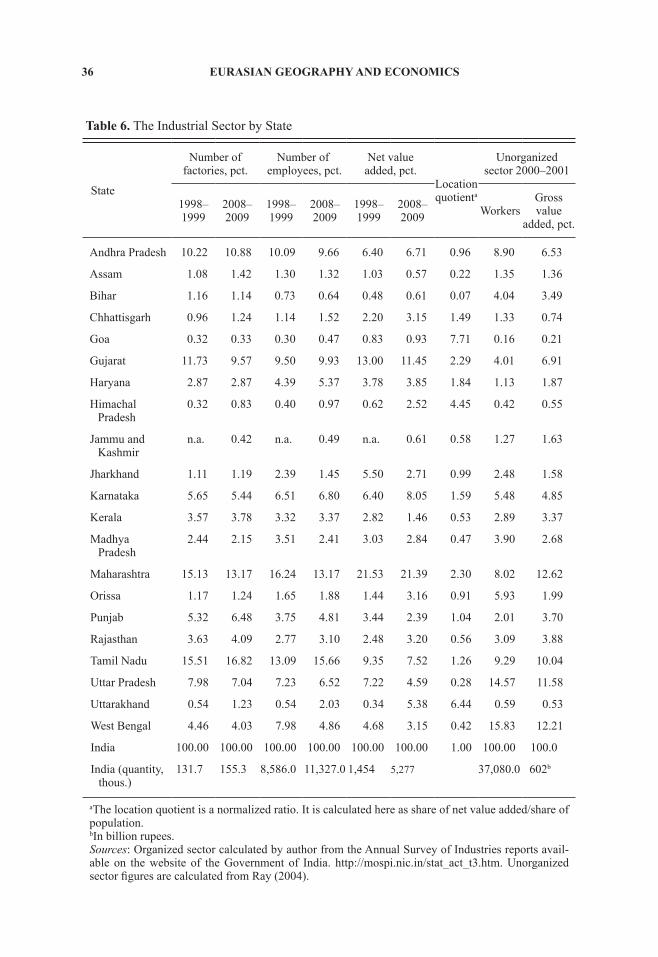
The leading industrial states were identified earlier in this paper, and the numbers in Table 6 confirm this earlier assessment using two sets of data. The first set covers the orga-nized industrial sector and includes factories registered under the Factories Act of 1948,14 and the second covers the unorganized sector (i.e., small or otherwise unregistered industrial or manufacturing units). It is useful to compare the two sectors using the 1998–1999 data for the organized sector, which is chronologically sufficiently close to the 2000–2001 data for the unorganized sector to be comparable. The total number of workers in the country’s organized sector in 1998–1999 was 8.6 million, only roughly one-fourth the 37 million in the unorganized sector. However, when the values of the two sectors’ output are compared, the organized sector outproduced its counterpart by more than a factor of two. This suggests that productivity in the organized sector is an order of magnitude higher.

The regional distribution of activity in the two sectors is also somewhat different. Maharashtra and Gujarat are the clear leaders in value addition in the organized sector, while Karnataka, Tamil Nadu, and Andhra Pradesh form a solid second tier. In terms of the number of employees, however, Tamil Nadu and Maharashtra are the frontrunners, with Gujarat and Andhra Pradesh forming the second tier. The location quotient, which here compares the dis-tribution of industry’s net value added to that of population, shows that Goa, Uttarakhand, and Himachal Pradesh have value added from organized industries that far exceeds their popula-tion base. Bihar and Uttar Pradesh, conversely, have far less industrial output than their shares of India’s total population would suggest.15

In the unorganized sector, Maharashtra and Tamil Nadu continue to be important, but two different states, West Bengal and Uttar Pradesh, are equally significant. These four states account for almost half of the country’s entire unorganized industrial workforce and close to half the value added in the sector. Gujarat, Andhra Pradesh, and Karnataka also appear sig-nificant, but less so than they are in the organized sector. Himachal Pradesh and Uttarakhand, which have disproportionately large organized industries, are almost insignificant as locations for unorganized industry.

Thus, the picture revealed by considering both the organized and unorganized industrial sectors is more complicated than that presented in most analyses, which tends to cover the data-rich organized sector. The leading edge of high-value, large-scale industry in India is undoubtedly found in Maharashtra and Gujarat, but industry as a whole is more widely dis-tributed, so that Tamil Nadu, West Bengal, and Uttar Pradesh also are important states, as are Karnataka and Andhra Pradesh.

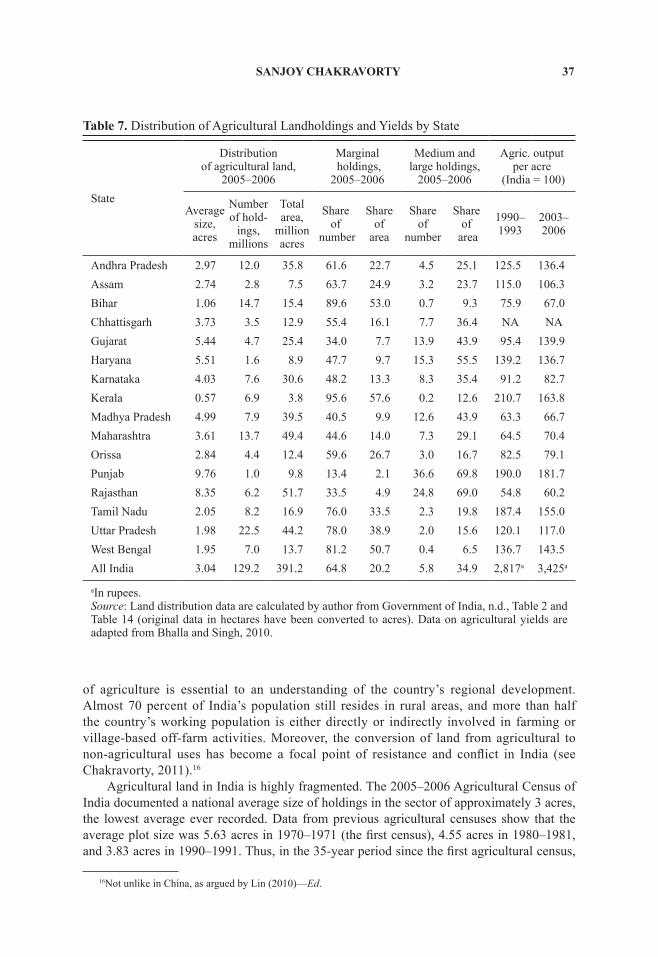
The final set of data examined here is devoted to Indian agriculture (Table 7). The regional development literature tends to ignore this sector because its value added is low, and the point of “development” is to move away from agriculture into manufacturing and services. These arguments notwithstanding, basic knowledge of the regional distribution

13It includes activities as diverse as finance, information technology, and other knowledge work (at the high end) as well as domestic servants and petty transport workers and shopkeepers.

14These data are reported in India’s Annual Survey of Industries (ASI). 15Bihar, for instance, has only 7 percent of the value addition in organized industry that would have been pre-

dicted if the organized industrial sector were evenly spread across India’s states.


Table 6. The Industrial Sector by State

State

Number of factories, pct.

Number of employees, pct.

Net value added, pct.

Location quotienta

Unorganized sector 2000–2001

1998–1999

2008–2009

1998–1999

2008–2009

1998–1999

2008–2009 Workers

Gross value

added, pct.

Andhra Pradesh 10.22 10.88 10.09 9.66 6.40 6.71 0.96 8.90 6.53

Assam 1.08 1.42 1.30 1.32 1.03 0.57 0.22 1.35 1.36

Bihar 1.16 1.14 0.73 0.64 0.48 0.61 0.07 4.04 3.49

Chhattisgarh 0.96 1.24 1.14 1.52 2.20 3.15 1.49 1.33 0.74

Goa 0.32 0.33 0.30 0.47 0.83 0.93 7.71 0.16 0.21

Gujarat 11.73 9.57 9.50 9.93 13.00 11.45 2.29 4.01 6.91

Haryana 2.87 2.87 4.39 5.37 3.78 3.85 1.84 1.13 1.87

Himachal Pradesh

0.32 0.83 0.40 0.97 0.62 2.52 4.45 0.42 0.55

Jammu and Kashmir

n.a. 0.42 n.a. 0.49 n.a. 0.61 0.58 1.27 1.63

Jharkhand 1.11 1.19 2.39 1.45 5.50 2.71 0.99 2.48 1.58

Karnataka 5.65 5.44 6.51 6.80 6.40 8.05 1.59 5.48 4.85

Kerala 3.57 3.78 3.32 3.37 2.82 1.46 0.53 2.89 3.37

Madhya Pradesh

2.44 2.15 3.51 2.41 3.03 2.84 0.47 3.90 2.68

Maharashtra 15.13 13.17 16.24 13.17 21.53 21.39 2.30 8.02 12.62

Orissa 1.17 1.24 1.65 1.88 1.44 3.16 0.91 5.93 1.99

Punjab 5.32 6.48 3.75 4.81 3.44 2.39 1.04 2.01 3.70

Rajasthan 3.63 4.09 2.77 3.10 2.48 3.20 0.56 3.09 3.88

Tamil Nadu 15.51 16.82 13.09 15.66 9.35 7.52 1.26 9.29 10.04

Uttar Pradesh 7.98 7.04 7.23 6.52 7.22 4.59 0.28 14.57 11.58

Uttarakhand 0.54 1.23 0.54 2.03 0.34 5.38 6.44 0.59 0.53

West Bengal 4.46 4.03 7.98 4.86 4.68 3.15 0.42 15.83 12.21

India 100.00 100.00 100.00 100.00 100.00 100.00 1.00 100.00 100.0

India (quantity, thous.)

131.7 155.3 8,586.0 11,327.0 1,454 5,277 37,080.0 602b

aThe location quotient is a normalized ratio. It is calculated here as share of net value added/share of population.bIn billion rupees.Sources: Organized sector calculated by author from the Annual Survey of Industries reports avail-able on the website of the Government of India. http://mospi.nic.in/stat_act_t3.htm. Unorganized sector figures are calculated from Ray (2004).


of agriculture is essential to an understanding of the country’s regional development. Almost 70 percent of India’s population still resides in rural areas, and more than half the country’s working population is either directly or indirectly involved in farming or village-based off-farm activities. Moreover, the conversion of land from agricultural to non-agricultural uses has become a focal point of resistance and conflict in India (see Chakravorty, 2011).16

Agricultural land in India is highly fragmented. The 2005–2006 Agricultural Census of India documented a national average size of holdings in the sector of approximately 3 acres, the lowest average ever recorded. Data from previous agricultural censuses show that the average plot size was 5.63 acres in 1970–1971 (the first census), 4.55 acres in 1980–1981, and 3.83 acres in 1990–1991. Thus, in the 35-year period since the first agricultural census,

16Not unlike in China, as argued by Lin (2010)—Ed.

Table 7. Distribution of Agricultural Landholdings and Yields by State

State

Distribution of agricultural land,

2005–2006

Marginal holdings,

2005–2006

Medium and large holdings,

2005–2006

Agric. output per acre

(India = 100)

Average size, acres

Number of hold-

ings, millions

Total area,

million acres

Share of

number

Share of

area

Share of

number

Share of

area

1990–1993

2003–2006

Andhra Pradesh 2.97 12.0 35.8 61.6 22.7 4.5 25.1 125.5 136.4Assam 2.74 2.8 7.5 63.7 24.9 3.2 23.7 115.0 106.3Bihar 1.06 14.7 15.4 89.6 53.0 0.7 9.3 75.9 67.0Chhattisgarh 3.73 3.5 12.9 55.4 16.1 7.7 36.4 NA NAGujarat 5.44 4.7 25.4 34.0 7.7 13.9 43.9 95.4 139.9Haryana 5.51 1.6 8.9 47.7 9.7 15.3 55.5 139.2 136.7Karnataka 4.03 7.6 30.6 48.2 13.3 8.3 35.4 91.2 82.7Kerala 0.57 6.9 3.8 95.6 57.6 0.2 12.6 210.7 163.8Madhya Pradesh 4.99 7.9 39.5 40.5 9.9 12.6 43.9 63.3 66.7Maharashtra 3.61 13.7 49.4 44.6 14.0 7.3 29.1 64.5 70.4Orissa 2.84 4.4 12.4 59.6 26.7 3.0 16.7 82.5 79.1Punjab 9.76 1.0 9.8 13.4 2.1 36.6 69.8 190.0 181.7Rajasthan 8.35 6.2 51.7 33.5 4.9 24.8 69.0 54.8 60.2Tamil Nadu 2.05 8.2 16.9 76.0 33.5 2.3 19.8 187.4 155.0Uttar Pradesh 1.98 22.5 44.2 78.0 38.9 2.0 15.6 120.1 117.0West Bengal 1.95 7.0 13.7 81.2 50.7 0.4 6.5 136.7 143.5All India 3.04 129.2 391.2 64.8 20.2 5.8 34.9 2,817a 3,425a

aIn rupees.Source: Land distribution data are calculated by author from Government of India, n.d., Table 2 and Table 14 (original data in hectares have been converted to acres). Data on agricultural yields are adapted from Bhalla and Singh, 2010.


mean plot size has decreased by almost one-half. Furthermore, these national averages mask quite significant state-to-state and within-state variation in plot size. Some states (especially Kerala and Bihar) have fragmented, very small holdings. Others (Punjab, Rajasthan, Haryana, Gujarat, and Madhya Pradesh, in descending order) have much larger, more consolidated ones. These latter states have only a small portion of their lands in “marginal holdings” (defined as plots smaller than 2.5 acres).

In Kerala, where over 95 percent of all landholdings are marginal, the average plot size is 0.57 acres. In Bihar, where almost 90 percent of holdings are marginal, the average hold-ing size is roughly 1 acre. Even in Tamil Nadu, Uttar Pradesh, and West Bengal, over three-fourths of all landholdings are designated as marginal. It may be fair to say that the political economy of these states is largely driven by this extremely fragmented distribution of agri-cultural land—i.e., the interests of marginal and small rural landholders. Conversely, less than 6 percent of all landholdings in the country account for almost 35 percent of all agricultural land. Therefore, in states with large holdings (Punjab, Rajasthan, Haryana, Gujarat), it can be argued that the interests of larger farmers is a key driver of state policy.

The states with highly fragmented land, with the exception of Bihar, are also among the leaders in agricultural output per acre. Other productivity leaders are states where land is relatively plentiful (or at least less fragmented) and the majority is held in medium and large plots. These include Punjab and Haryana, which are considered India’s agricultural leaders, with Gujarat possibly a late entrant into this club. But large landholdings do not guarantee high output; Rajasthan and Madhya Pradesh, with among the largest average hold-ings, offer difficult agricultural terrains and two of the lowest productivity figures. Similarly, Maharashtra’s landholding size is higher than the national average but its productivity is much lower. Therefore, just as the industrial sector yields surprises when both its organized and unorganized elements are considered, so the agricultural sector presents all combinations of land fragmentation and productivity: high fragmentation–high productivity, high fragmen-tation–low productivity, low fragmentation–high productivity, and low fragmentation–low productivity.

THE POTENTIAL FOR DISTRICT-LEVEL ANALYSIS

In the introduction, I observed that many states in India are so large that state-level analy-sis may be inappropriate to an understanding of regional development processes and out-comes—that it may be more useful to look at district level outcomes. This is not a new idea. In fact, the Indian government has attempted since 1960 to identify “backward” districts,17 and such attempts continue to this day. In 1997, the Sarma Committee identified the 100 most lagging districts in the country, including 38 in Bihar (before Jharkhand was created), 19 in Madhya Pradesh (before Chhattisgarh was created), 17 in Uttar Pradesh (before Uttarakhand was created), and 10 in Maharashtra. No such districts were identified in the states of Gujarat, Goa, Kerala, Punjab, Andhra Pradesh, and Tamil Nadu.18 In 2002, the Planning Commission created a list of 100 lagging districts, and another list of 177 lagging districts in 2005.19 Indi-vidual states have their own lists of lagging districts and have created tax and other incentives to direct industrial investment into them, with little success to date.

17This is the official term; here I use “lagging” districts.18Jammu and Kashmir and the northeastern states were not considered as they had “peculiar” issues—namely,

insurgencies.19All three lists (the Sarma and two Planning Commission lists) are cited in Planning Commission (2005).


Several non-government efforts also have been initiated to identify lagging districts. Debroy and Bhandari (2003) created their own list of 69 lagging districts, and The World Bank (2011) has undertaken a series of poverty-mapping exercises in eastern India. Jalan and Ravallion (1997) have written extensively about “spatial poverty traps” in Indian dis-tricts, and Chakravorty (2000) identified clusters of districts that receive little or no industrial investment. Many analysts, including those employed by the Government of India, agree that there is a significant overlap between the concentration of tribals (the country’s historically socially marginalized groups) and lagging districts.

Maharashtra provides a good example of the magnitude of variance in living standards that is possible at the intra-state and intra-metropolitan levels. At one end there is Mumbai, an aspiring global city, the hub of India’s financial and entertainment sectors, a major manufac-turing base and port, with the highest land costs and per capita incomes in the country. At the same time, Mumbai is home to Asia’s largest slum (Dharavi, where about 1 million people live); it is estimated that over 40 percent, perhaps as much as 45 percent of the metropolitan population lives in slums. Maharashtra itself has identified 14 districts as lagging, including Parbhani, Yavatmal, and Gadchiroli, which are among the poorest in the country. Similar intra-state variances are evident in states such as Uttar Pradesh (highly developed Noida in the greater Delhi region versus many impoverished districts in the southern and eastern parts of the state) and West Bengal (developed Kolkata versus Puruliya, Birbhum, and districts farther north).

Variance in development indicators (on income or poverty or any of the other variables considered above) is undoubtedly higher at the district level than at the state level. This is to be expected because spatial disaggregation increases spatial variance. But whether these dis-trict-level variances are increasing or decreasing over time cannot be determined with much certainty. Some of the indeterminacy arises from differences in the variables themselves, and some of it results from issues of scale. For instance, it is quite possible that decreasing intra-state inequality in manufacturing output is occurring at the same time that there is increasing intra-national inequality in manufacturing output at the district level (Chakravorty, 2000). But it is equally possible to find that for other variables (such as poverty) there is increasing intra-state inequality accompanied by decreasing intra-national inequality. What the observer sees depends on the variable, the scale, and the range of units under observation. Remember: the story of the blind men and the elephant originated in India.

EXPLANATION

Broadly considered, there are two theoretical approaches to understanding changes in comparative regional development (or regional inequality) over time—from separate traditions in economics and geography. Let us briefly consider the principal strands in these approaches and test them against the regional reality of India presented above. This review is quite brief, and for this reason may be overly reductive and simplistic.

The oldest economic approach to studying comparative regional development over the long run stems from the work of Gunnar Myrdal (1957) and Albert Hirschman (1958). Both argued for an initial period of “cumulative causation” (Myrdal) or “polarization” (Hirschman), during which, because of increasing returns to scale and positive externalities in industrial growth, leading regions would move farther ahead of the rest. These initial advantages would eventually decline, there would be diminishing returns, political demands would arise from the lagging regions, etc.—all of which would lead to “backwash” or “polarization reversal.” These ideas were empirically investigated by Jeffrey Williamson (1965) who extended the


work of Simon Kuznets (1955) on income inequality to the regional domain. Williamson argued that regional inequality would increase and then decline through the process of devel-opment—divergence followed by convergence—drawing the now famous inverted-U curve. There have been numerous tests of the Williamson thesis, with Alonso (1980) arguing that it was one of five “stylized facts” of development.

More recently, following the endogenous growth literature and stressing the idea of diminishing returns, Robert Barro and Xavier Sala-i-Martin (1992, 1995) have argued for two types of regional convergence over the long term. When the divergence of real per capita income across a group of economies decreases over time, there is σ-convergence. And when the partial correlation between growth in income over time and its initial level is negative, there is β-convergence. Empirical tests of these ideas have generally been successful using North American and European data (σ-convergence is viewed as more likely), but less so with data from the rest of the world (Milanovic, 2005).

Geographical approaches to the regional development question have generally proceeded in two directions. One has highlighted the importance of scale. Much depends on how a region is defined (administrative boundaries may be convenient data holders but may not have much organic meaning). In the Indian case, are states appropriate units of measure-ment, or meta-regions consisting of several states, or districts, or clusters of districts? It is possible that divergence and convergence are scale-dependent rather than time- or variable-dependent (Chakravorty, 1994). The second geographical approach comes from the Marxist tradition exemplified in the works of David Harvey, Neil Smith, Richard Peet, and others (see Harvey, 1982; Smith, 1984). Here, comparative regional development does not necessarily have determinate outcomes because capitalists configure space to generate profit in ways that are dynamic and contingent. More recently, the “critical” discourse on regional development has been subsumed under the banner of “neoliberalism,” which appears to suggest that inter-regional divergence is the most likely outcome of neoliberal policies enacted by governments for the benefit of private capital.

I suggest that our just-concluded examination of the recent evidence on regional perfor-mance in India could lead us to accept (or reject) all of these approaches. There is evidence favoring divergence caused by cumulative causation if one looks at the continued growth of the organized industrial sector in Gujarat and Maharashtra. There is divergence in per capita “income,” at least until the mid-2000s, especially if Bihar is used as the basis of comparison. But, at the same time, if we examine the growth rate of state domestic product over the last two plan periods (plus the current, ongoing one), several low-income states, including Bihar, have outperformed many high income ones. And if the focus shifts to the formation of the unorganized industrial sector, one can see that it is far more evenly spread, especially in middle- and low-income states, than the data on the organized sector would suggest. For the organized industrial sector, a deeper probing into its history reveals an extreme concentration in the early 1900s, with up to three-quarters of all industry concentrated in the then-leading centers of Calcutta, Bombay, and Madras (Awasthi, 1991); yet there is no doubt that industry has and continues to spread far beyond those initial concentrations. Similar notes of disso-nance are evident in the data on agriculture, where the acknowledged leaders (Punjab and Haryana) are matched and even outperformed (in terms of output per acre) by states with very fragmented landholdings (Kerala and West Bengal).

The long history of regional development in India (not covered here) also provides sup-port for both divergence and convergence. Evidence supporting the former can be found in the example of Bihar’s steady backward slide in SDP relative to the leading states and the


Indian average.20 This is tempered, however, by more recent growth rates that suggest that Bihar is now outperforming the leading states. But more important is the fluctuating identity of India’s “leading state” through the decades, the antipodal state with which Bihar is com-pared. At independence it was West Bengal, now only a middle-rung state with an average income below that of India as a whole. It was succeeded, after the Green Revolution, by Punjab, a state that has now been in relative decline for at least two decades, its growth rate consistently below the Indian average, and among the lowest in the country. Punjab’s decline allowed Maharashtra to become the leading state based on strong industrial growth. But over the past decade Maharashtra appears to have been overtaken by Gujarat,21 based again on strong industrial growth.

There is turbulence at the top. The leading states of past decades have converged toward the middle and different states have taken their place. Even the bottom has been unsteady. Not long ago, it was common to discuss the pathologies of the BIMARU states of Bihar, Madhya Pradesh, Rajasthan, and Uttar Pradesh.22 Rajasthan no longer belongs in this group, and with Jharkhand, Chhattisgarh, and Uttarakhand having been created out the remaining three states, the BIMARU terminology no longer has meaning. It may be more appropriate to think of an area starting from central Uttar Pradesh, stretching through all of Bihar, Jharkhand, Orissa, Chhattisgarh, and into eastern Madhya Pradesh as India’s “heart of darkness.” This is where poverty is concentrated (although it exists in districts across the nation, especially in Maharashtra and West Bengal), human development is low, and capital investment (other than in extractive industries) meager. Yet, even these districts have lowered poverty and elevated their human development indicators over the past two decades. And starting from a low base, small gains in these regions appear more impressive than equal gains in already developed regions such as Goa or Kerala.

It is necessary to look beyond the numbers and scale effects and the straightjacket of theory. Once we do, it is clear that “history matters” and “governance matters.” Banerjee and Iyer (2005) and Kapur and Kim (2006) have shown that regional development outcomes (especially agricultural performance) in independent India can be substantially explained by the land revenue extraction system used by the British colonizers in the 18th and 19th centu-ries. I have recently argued that because the British revenue extraction system was largely an extension of pre-colonial systems, it is even possible to see the long shadow of 16th and 17th century India in regional performance today (Chakravorty, 2011). History matters because institutions, laws, and norms matter. They condition individual and group behavior and class relations and conflict. These are the fundamentals that lead to production and consumption and economic and social development—i.e., the variables we attempt to measure in an effort to understand what is going on.

The institution of governance matters perhaps more than anything else, especially in developmental states where government is the most important institution. Government makes, enforces, and extracts rents from the policies and rules that direct the economic and social life of its citizens. The importance of regional governance has been underlined by the recent expe-rience of Bihar, where a “developmental” government headed by a reformer (Nitish Kumar) appears to have pulled the state out of its nosedive, a condition that had been worsened by the previous long-term governance of Lalu Yadav and his “populist” government that was widely known for corruption and inefficiency. The importance of governance is highlighted also by

20Recall that at independence the leading state’s income was 2.5 times that of Bihar, whereas by 2007–2009 it was five times higher (Table 2).

21I am ignoring Goa in this discussion.22BIMARU is an acronym of the state names that plays on the Hindi word “bimar” (ill).


the contrasting experiences in Kerala and West Bengal, both ruled by communist parties for long stretches, but with starkly different outcomes—inclusive and generative in Kerala, par-tisan and autocratic in West Bengal.

I end with a note of dissent on regional development theory. Both increasing and dimin-ishing returns are possible, simultaneously. Cumulative causation is a real possibility in many settings and can persist for extended periods, but cities and metropolises can become too expensive to carry out many types of work efficiently, and new work can and does seek new locations. The state in India is not one thing—neoliberal or pro-business or pro-poor or redistributive. It is all of these things, simultaneously. Therefore, simple explanations are not possible. We encounter complexity and contradiction in every sphere. Regional development in India is no exception.

REFERENCES

Alonso, W., “Five Bell Shapes in Development,” Papers of the Regional Science Association, 45, 1:5–16, 1980.

Awasthi, D., Regional Patterns of Industrial Growth in India. New Delhi, India: Concept Publishing, 1991.

Banerjee, A. and L. Iyer, “History, Institutions and Economic Performance: The Legacy of Colonial Land Tenure Systems in India,” American Economic Review, 95, 4:1190–1213.

Barro, R. J. and X. Sala-i-Martin, “Convergence,” Journal of Political Economy, 100, 2:223–51, 1992.

Barro, R. J. and X. Sala-i-Martin, Economic Growth. New York, NY: McGraw Hill, 1995.Bhalla, G. S. and G. Singh, Growth of Indian Agriculture: A District Level Study. New Delhi, India:

Planning Commission, Government of India, 2010 (mimeo).“Bihar to Outpace its Own Growth Rate This Fiscal: Nitish,” Times of India, October 16, 2011.Chakravorty, S., The Price of Land: Acquisition and Conflict in India, 2011 (in progress).Chakravorty, S., “How Does Structural Reform Affect Regional Development? Resolving Contradic-

tory Theory with Evidence from India,” Economic Geography, 76, 4:367–394, 2000.Chakravorty, S., “Equity and the Big City,” Economic Geography, 70, 1:1–22, 1994.Chakravorty, S. and S. V. Lall, Made in India: The Economic Geography and Political Economy of

Industrialization. New Delhi, India: Oxford University Press, 2007.Debroy, B. and L. Bhandari, District-Level Deprivation in the New Millennium. New Delhi, India:

Konark Publishers, 2003.Dehejia, J., “Economic Reforms: Birth of an ‘Asian Tiger’,” in P. Oldenburg, ed., India Briefing.

Boulder, CO: Westview, 1993, 75–102.Government of India, Ministry of Home Affairs, “Provisional Population Totals Paper 2 of 2011 in

India,” 2011 [http://www.censusindia.gov.in/2011-prov-results/paper2/prov_results_paper2_india .html], last accessed January 11, 2012.

Government of India, Press Information Bureau, “Poverty Estimates for 2004–2005,” March 2007 [http://planningcommission.nic.in/news/prmar07.pdf], last accessed January 12, 2002.

Government of India, Department of Agriculture and Cooperation, Agriculture Census 2005–2007, n.d. [http://agcensus.nic.in/document/agcensus2005/agcen2005rep.htm], last accessed January 12, 2011.

Harvey, D., Limits to Capital. Oxford, UK: Basil Blackwell, 1982. Hirschman, A. O., The Strategy of Economic Development. New Haven, CT: Yale University Press,

1958.Jalan, J. and M. Ravallion, Spatial Poverty Traps? Washington, DC: World Bank, Development

Research Group Working Paper No. 1862, 1997.Kapur, S. and S. Kim, British Colonial Institutions and Economic Development in India. Cambridge,

MA: National Bureau of Economic Research Working Paper No. w.12613, 2006.


Kundu, A. and K. Varghese, Regional Inequality and “Inclusive Growth” in India under Globaliza-tion: Identification of Lagging States for Strategic Intervention. New Delhi, India: Oxfam India Working Paper Series, 2010.

Kuznets, S., “Economic Growth and Income Inequality,” American Economic Review, 45, 1:1–28, 1955.

Lin, G. C. S., “Understanding Land Development Problems in Globalizing China,” Eurasian Geogra-phy and Economics, 51, 1:80–103, 2010.

Lin, G. C. S. and F. Z. Y. Hu, “Getting the China Story Right: Insights from National Economic Censuses,” Eurasian Geography and Economics, 52, 5:712–746, 2011.

“Mayawati Bursts Narendra Modi’s Economic Growth Myth,” Times of India, October 22, 2011.Milanovic, B., Worlds Apart: Measuring International and Global Inequality. Princeton, NJ: Princeton

University Press, 2005.Myrdal, G., Economic Theory and Underdeveloped Regions. London, UK: Duckworth, 1957.Planning Commission, Report of the Inter-Ministry Task Group on Redressing Growing Regional

Imbalances. New Delhi, India: Planning Commission, 2005 [http://planningcommission.nic.in/aboutus/taskforce/inter/inter_reg.pdf ], last accessed January 24, 2012.

Ray, N., Unorganized vis-à-vis Organized Manufacturing Sector in India. New Delhi, India: Govern-ment of India, Ministry of Statistics and Programme Implementation, 2004 (mimeo).

Satthertwaite, D., “Sustainable Cities or Cities that Contribute to Sustainable Development?,” Urban Studies, 34, 10:1667–1691, 1997.

Sen, A. K., Commodities and Capabilities. Amsterdam, The Netherlands: North Holland, 1985.Singh, N., J. Kendall, R. K. Jain, and J. Chander, Regional Inequality in India in the 1990s: Trends

and Policy Implications. Mumbai, India: Development Research Group, Reserve Bank of India, n.d. (mimeo).

Smith, N., Uneven Development: Nature, Capital, and the Production of Space. Athens, GA: University of Georgia Press, 1984.

Williamson, J. G., “Regional Inequality and the Process of National Development,” Economic Devel-opment and Cultural Change, 13, 1:3–45, 1965.

World Bank, Perspectives on Poverty in India: Stylized Facts from Survey Data. Washington, DC: The World Bank, 2011.

Documents

Regional Development in India: Paradigms Lost in a … Geography and Economics, 2012, 53, ... Paradigms Lost in a Period of Great Change ... The number of districts changes frequently