Embed Size (px)
Citation preview
Regional variations in labor demand
elasticity: evidence from U.S. counties
Abhradeep Maiti
Assistant Professor (Economics)
Indian Institute of Management Kashipur
and
Debarshi Indra
Senior Manager-Economic Research
Nielsen India
Abstract
We use a large panel dataset covering the period 1988-2010 to estimate county specific
own-wage elasticity of labor demand in the United States for four highly aggregated industries:
construction, finance/insurance/real-estate/ service, manufacturing, and retail trade. Our
estimation of a random parameter panel data model yields significant evidence of spatial
variations in wage elasticity of labor demand. We relate the spatial variation in elasticity to
differences in county characteristics like industry specialization, industry competition, levels of
natural amenity and urbanization. Using a regression discontinuity approach we also find that
pro-business states have higher labor demand elasticity.
Keywords: Control function, labor demand elasticity, random parameter model, right to work
law.
Acknowledgments: Debarshi Indra acknowledges the support of the Multi-campus Research
Program and Initiative (MRPI) grant from the Office of the President, University of California
(award number 142934). Views expressed in the article are solely those of the authors and not of
the financial supporters or the authors' affiliations. The authors are grateful to Alex Anas, E.
Anthon Eff, Daniel Hamermesh, Thomas Holmes, Peter Morgan, Mark D. Partridge, Neel Rao,
Joachim Zietz, and three anonymous referees for valuable comments and suggestions. The
authors are however solely responsible for any errors.

1
1. Introduction
The estimation of wage elasticity of labor demand has attracted significant attention in
empirical labor economics. Hamermesh (1993) provides an exhaustive review of the early
research in this field. A more recent survey can be found in Lichter, Peichi, and Siegloch (2014)
who tabulate 151 studies conducted between 1980 and 2012 on 37 different countries. Most
studies listed in these articles estimate wage elasticity of labor demand for one sector or industry,
in particular the manufacturing sector, and assume no spatial variation in elasticity. In this paper
we document spatial heterogeneity in U.S. labor demand elasticity by estimating industry-county
elasticity for four aggregated industries1: construction, finance/insurance/real-estate/service,
manufacturing, and retail trade. There are other studies which also find significant spatial
heterogeneity in U.S. labor market outcomes. For example, after a comprehensive survey of the
local labor market literature, Moretti (2011) catalogs spatial variations in nominal wages, real
wages, productivity, and innovation across U.S. labor markets. He also finds evidence that these
variations have persisted over many decades.
We use a large panel dataset based on the County Business Patterns and a two-step
procedure to estimate industry-county labor demand elasticity. In step-one we specify a random
parameter panel data model, where we assume that industry-county labor demand elasticity is not
constant, but has a lognormal distribution in the population of counties. The lognormal
distribution ensures that the absolute value of labor demand elasticity is always positive. We
estimate the parameters of this model using the method of Maximum Simulated Likelihood
(MSL). Once we have information regarding the distributions of labor demand elasticity, in step-
1 Together these four industries account for-on average-about 87 percent of annual employment
in the private non-farm sector in the U.S.

2
two, we retrieve county level estimates using Bayes’ rule. We believe that this two-step approach
provides an alternative method for estimating spatially heterogeneous parameters2. In the extant
literature on labor demand elasticity—variation in elasticity is usually introduced either by
estimating separate regression models on subsets of data (Slaughter, 2001), or by interacting the
elasticity parameter with some spatially heterogeneous variable (Hasan et al., 2007). In our
approach, we do not need to subset our data in estimation, and more importantly, we do not need
to make any assumption regarding which variable to interact with the elasticity parameter. A
drawback of our approach is that it is computationally more challenging than linear models; plus
we also need to make an assumption regarding the distribution of parameters.
The labor demand elasticity in the four industries are distributed lognormal with the
following means and standard deviations3: 0.15 (0.13) for construction, 0.005 (0.05) for
finance/insurance/real-estate/service, 0.21 (0.38) for manufacturing and 0.09 (0.25) for retail
trade. We find that the scale parameter of the lognormal distribution is statistically significant for
all four industries which confirm the presence of spatial heterogeneity in labor demand elasticity.
How do our results compare with existing estimates in the literature on labor demand elasticity?
Lichter, Peichi, and Siegloch (2014) report a mean value of 0.50 (0.77) for overall labor demand
elasticity. In their analysis they classify elasticity estimates based on a number of factors—time
period, dataset, workforce, industry, and country; and report mean values for each group. In the
short-run, the mean value of elasticity is 0.21 (0.40) while in the long-run it is 0.34 (0.47). At the
industry level the mean value of elasticity is 0.53 (0.49), 0.04 (0.20), and 0.05 (0.23) in the
2A popular and widely used nonparametric method that deals with estimation of spatially
heterogeneous parameters is called Geographically Weighted Regression (GWR) (Brunsdon et
al., 1996). McMillen (2010) summarizes the application of GWR and other parametric and semi-
parametric methods in regional science and urban economics. 3Standard deviation in parenthesis.

3
manufacturing, service, and construction sectors respectively. They do not report any estimates
for the retail trade sector. Our average elasticity estimates for all the industries fall in the ranges
reported in Lichter, Peichi, and Siegloch (2014) albeit they are on the lower side of the ranges.
Our county level estimates of labor demand elasticity allow us to test if they are related to
other features of the spatial landscape of the U.S. economy. In particular, we test if labor demand
elasticity can be classified on the basis of natural amenity, industry-county specialization and
competition, urbanization, and government policies (Glaeser et al., 1992; Holmes and Stevens,
2004). Our findings can be summarized as follows:
(1) Counties with better natural amenity have higher labor demand elasticity.
(2) More industry-county specialization and competition reduces labor demand elasticity.
(3) Urbanization and labor demand elasticity is negatively related.
(4) Counties which belong to more pro-business states have higher labor demand
elasticity.
The last result is found using a regression discontinuity design described in Holmes (1998)4,
where pro-business states are defined as those states which have adopted the right-to-work law.
Our findings have important policy implications. In the U.S., Federal, State, and Local
governments intervene—in a variety of ways—in labor markets. For example, wage subsidy
programs seek to boost earnings and employment among the weaker sections of society (Katz,
1996). In addition, State and Local governments implement policies to try and attract firms by
providing them a variety of incentives, to either relocate, or open a new establishment in their
jurisdiction. Bartik (1991) provides a comprehensive list of such policies and Bartik (2002)
4We are grateful to Prof Thomas Holmes for sharing his data with us.

4
claims that these policies costs approximately 30-40 billion Dollars to implement. It is easy to
see in a partial equilibrium setting with perfectly elastic labor supply, that ceteris paribus, in
response to a wage subsidy program, counties with higher labor demand elasticity will generate
larger employment gains as compared to counties with lower labor demand elasticity. The entry
of a new firm and a subsequent output shock, will however, have the opposite effect, as labor
demand will rise more in a county with lower labor demand elasticity as compared to a county
with higher labor demand elasticity. This means that these policies need to be adjusted spatially
to generate similar effects across regions. In addition, the differential effect of output on
employment is also useful for investigating how employment levels in different regions reacts
differently during a recession5. Our results imply that differences in regional unemployment
levels might arise not only because different regions have different industry compositions, but
also because different regions have different labor demand elasticity.
Policy recommendations based on a partial equilibrium framework, however, can be
misleading, since we ignore the effects of other markets, in particular the housing market6. To
get accurate results we must rely on general equilibrium models. Partridge and Rickman (2010)
provide a thorough discussion on the increasing use of CGE models to assess local regional
development policies. Our industry-county labor demand estimates can be used to calibrate labor
demand functions in such CGE models and perform policy evaluations.
This paper proceeds as follows. In Section 2 we describe the data. Section 3 presents the
theory behind labor demand elasticity and outlines the estimation procedures. Section 4 discusses
5See Fingleton, Garretsen, and Martin (2012) and Curtis (2014) for a discussion of this issue. 6The Rosen-Roback (Rosen, 1979; Roback, 1982) model is a popular spatial general equilibrium
model which illuminates the tight link between the labor market and the housing market in a
region. See Glaeser and Gottlieb (2009) for a thorough discussion of the Rosen-Roback model.

5
the estimation results and classifies the elasticity estimates based on county and industry
characteristics mentioned earlier. We conclude in Section 5 by summarizing our results and
pointing to some future extension.
2. Data
We use the County Business Patterns (CBP) dataset from the period 1988 to 2010 to get
annual industry level data on total employees and total payroll for counties in the conterminous
U.S. Data in the CBP is available at various industry aggregation levels. For reasons we explain
below we use data based on the 2-digit industry classification system—this is the highest
industry aggregation level available in the CBP. We then further categorize (see Table 1) a
subset of these 2-digit industries into four major industry groups7—construction,
finance/insurance/real-estate/service, manufacturing, and retail trade.
The CBP has strength and weaknesses (Isserman and Westervelt, 2006). Its advantages are
that it is it is establishment8 based-making it ideal for spatial analysis, highly accurate9,
industrially detailed, and is available every year since 1964. The CBP, however, has its
drawbacks. For one thing, it does not include all employment10. In addition, the industry
classification system used in the CBP changes periodically. During 1988-2010, the CBP
followed two different industry classification systems—the Standard Industry Classification
(SIC) system for the period leading up to 1997 and the North American Industry Classification 7These four industry groups together account for 87 percent of total employment reported in the
CBP every year. We leave out agriculture, mining, transportation, and wholesale trade from our
analysis. 8 Establishments, according to the Census Bureau are physical locations of economic activity. 9 The accuracy of the CBP comes from the fact that it is based on administrative records of the
Internal Revenue Service, the Social Security Administration, and the Bureau of Labor Statistics. 10It covers private, nonfarm employment, but ignores agricultural production employees,
majority of government employees, self-employed individuals, employees of private households,
and railroad employees. It only counts full- and part-time employees on the payroll in the mid-
March period. This introduces a seasonal component in the data for certain industries.
6
System (NAICS) thereafter. However, the biggest problem with the CBP is data suppression due
to confidentiality reasons. This problem rises with industrial detail and in such cases the CBP
provides an interval for industry employment level, but sets payroll data equal to zero.
The choice of using the 2-digit industry classification system makes our industry
definition less sensitive to changes in the industry classification system but more importantly it
minimizes the effects of data suppression in our analysis. We now describe some statistics
regarding data suppression at the 2-digit industry level. In the construction industry 9 percent of
71,153 observations (an observation is a 2-digit industry-county-year combination) suffer from
data suppression and 96 percent of the missing data are from non-metro counties (see Appendix
A for definition of non-metro counties). The finance/insurance/real-estate/service industry has
400,534 observations, 21 percent of which have missing data, and 79 percent of the missing data
belong to non-metro counties. The manufacturing sector has 70,314 observations, 14 percent of
which have missing data, and 92 percent of the missing data belong to non-metro counties.
Finally, in the retail trade sector, 13 percent of 150,001 observations have missing data and 83
percent of the missing data belong to non-metro counties. The finance/insurance/real-
estate/service and retail trade industry groups have significantly larger number of observations
than the construction and manufacturing sectors since the former two are made up of
significantly more 2-digit industries (see Table 1).
While we lose a large number of observations due to data suppression, a more important
question for our empirical analysis is to know the number of industry employees we fail to
include due to missing data. In the CBP, while data suppression affects individual 2-digit
industries, it does not affect the reporting of total employment across all industries for a county-
7
year combination11. This allows us to calculate the number of employees we lose due to data
suppression. Our calculation shows that, on average, every year we lose about 1 percent of total
employment. This means that the observations with the missing employment data can be safely
dropped from our analysis without biasing our results—the remaining data set is able to capture
99 percent of all employment fluctuations recorded in the CBP. After dropping the observations
with missing employment data we aggregate the 2-digit industry data into our four major
industry groups based on the classification in Table 1. This yields a datasets consisting of
64,832; 70,166; 60,331; and 70,484 observations for the construction, finance/insurance/real-
estate/service, manufacturing, and retail trade industries respectively.
The industry datasets have an unbalanced panel structure as not all counties appear every
year in each industry dataset. The construction, finance/insurance/real-estate/service,
manufacturing, and retail trade datasets contain 3078, 3100, 2982, and 3103 distinct counties.
The average length of appearance for each county in these four datasets are 21, 22, 20, and 22
years respectively. In the period 1988-2010 there were 3114 distinct counties in the
conterminous U.S. implying that the industry datasets cover on average 98 percent of counties
and these counties on average appear 90 percent of the time. As mentioned earlier the counties
absent from the industry datasets are mostly non-metro counties with sparse employment levels.
The CBP follows the U.S. census definition for counties: the independent cities in Virginia
are treated as separate counties. This is unlike cities in other states which are part of the counties
in which they are located. Following Holmes (1998) we merge the independent cities in Virginia
with the counties that surround them—this definition of counties comes from the Regional
Economic Information System (REIS). This consolidation of cities in Virginia with surrounding
11As Isserman and Westervelt (2006) reports, in 2002, only 77,331 total jobs were subject to
suppression out of 112.4 million, a negligible quantity.
8
counties reduces the number of observations in the industry datasets. Now construction,
finance/insurance/real-estate/service, manufacturing, and retail trade have 64,051; 69,376;
59,578; and 66,648 observations respectively.
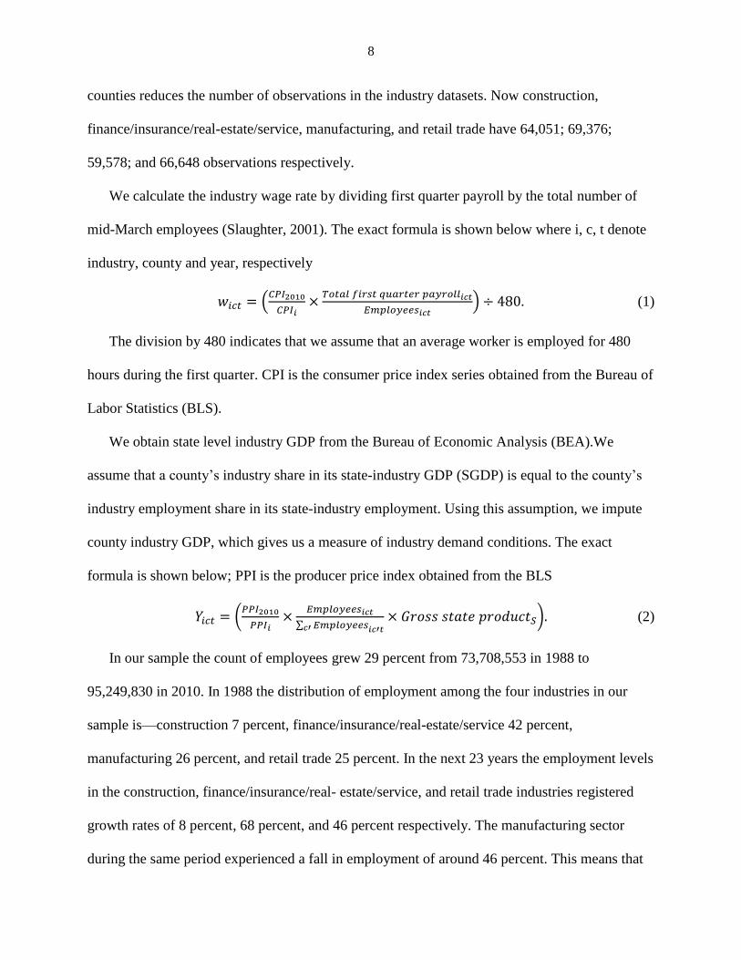
We calculate the industry wage rate by dividing first quarter payroll by the total number of
mid-March employees (Slaughter, 2001). The exact formula is shown below where i, c, t denote
industry, county and year, respectively
𝑤𝑖𝑐𝑡 = (𝐶𝑃𝐼2010
𝐶𝑃𝐼𝑖×𝑇𝑜𝑡𝑎𝑙 𝑓𝑖𝑟𝑠𝑡 𝑞𝑢𝑎𝑟𝑡𝑒𝑟 𝑝𝑎𝑦𝑟𝑜𝑙𝑙𝑖𝑐𝑡
𝐸𝑚𝑝𝑙𝑜𝑦𝑒𝑒𝑠𝑖𝑐𝑡) ÷ 480. (1)
The division by 480 indicates that we assume that an average worker is employed for 480
hours during the first quarter. CPI is the consumer price index series obtained from the Bureau of
Labor Statistics (BLS).
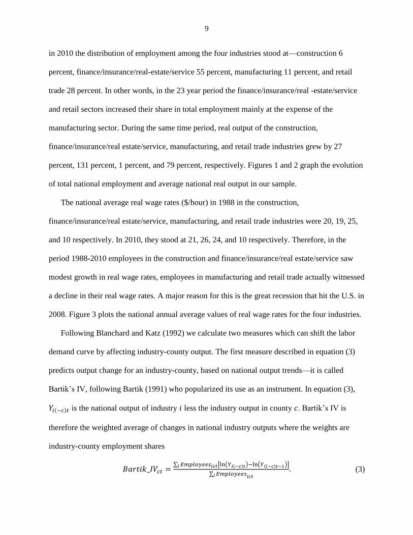
We obtain state level industry GDP from the Bureau of Economic Analysis (BEA).We
assume that a county’s industry share in its state-industry GDP (SGDP) is equal to the county’s
industry employment share in its state-industry employment. Using this assumption, we impute
county industry GDP, which gives us a measure of industry demand conditions. The exact
formula is shown below; PPI is the producer price index obtained from the BLS
𝑌𝑖𝑐𝑡 = (𝑃𝑃𝐼2010
𝑃𝑃𝐼𝑖×
𝐸𝑚𝑝𝑙𝑜𝑦𝑒𝑒𝑠𝑖𝑐𝑡
∑ 𝐸𝑚𝑝𝑙𝑜𝑦𝑒𝑒𝑠𝑐′ 𝑖𝑐′𝑡
× 𝐺𝑟𝑜𝑠𝑠 𝑠𝑡𝑎𝑡𝑒 𝑝𝑟𝑜𝑑𝑢𝑐𝑡𝑆). (2)
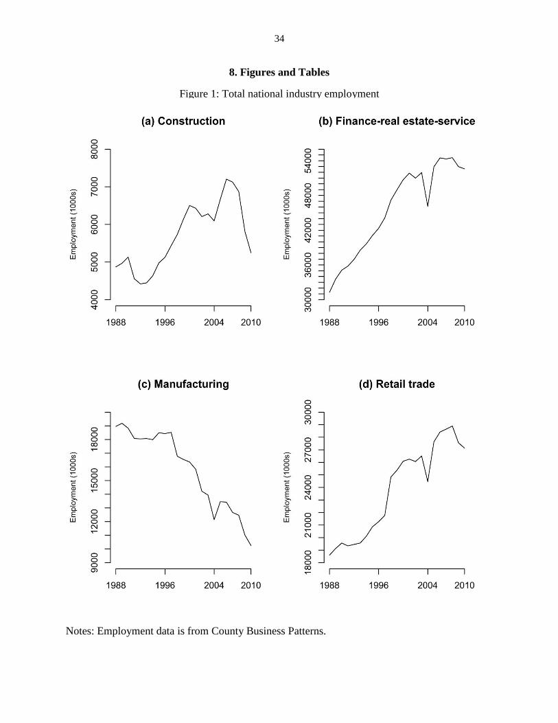
In our sample the count of employees grew 29 percent from 73,708,553 in 1988 to
95,249,830 in 2010. In 1988 the distribution of employment among the four industries in our
sample is—construction 7 percent, finance/insurance/real-estate/service 42 percent,
manufacturing 26 percent, and retail trade 25 percent. In the next 23 years the employment levels
in the construction, finance/insurance/real- estate/service, and retail trade industries registered
growth rates of 8 percent, 68 percent, and 46 percent respectively. The manufacturing sector
during the same period experienced a fall in employment of around 46 percent. This means that
9
in 2010 the distribution of employment among the four industries stood at—construction 6
percent, finance/insurance/real-estate/service 55 percent, manufacturing 11 percent, and retail
trade 28 percent. In other words, in the 23 year period the finance/insurance/real -estate/service
and retail sectors increased their share in total employment mainly at the expense of the
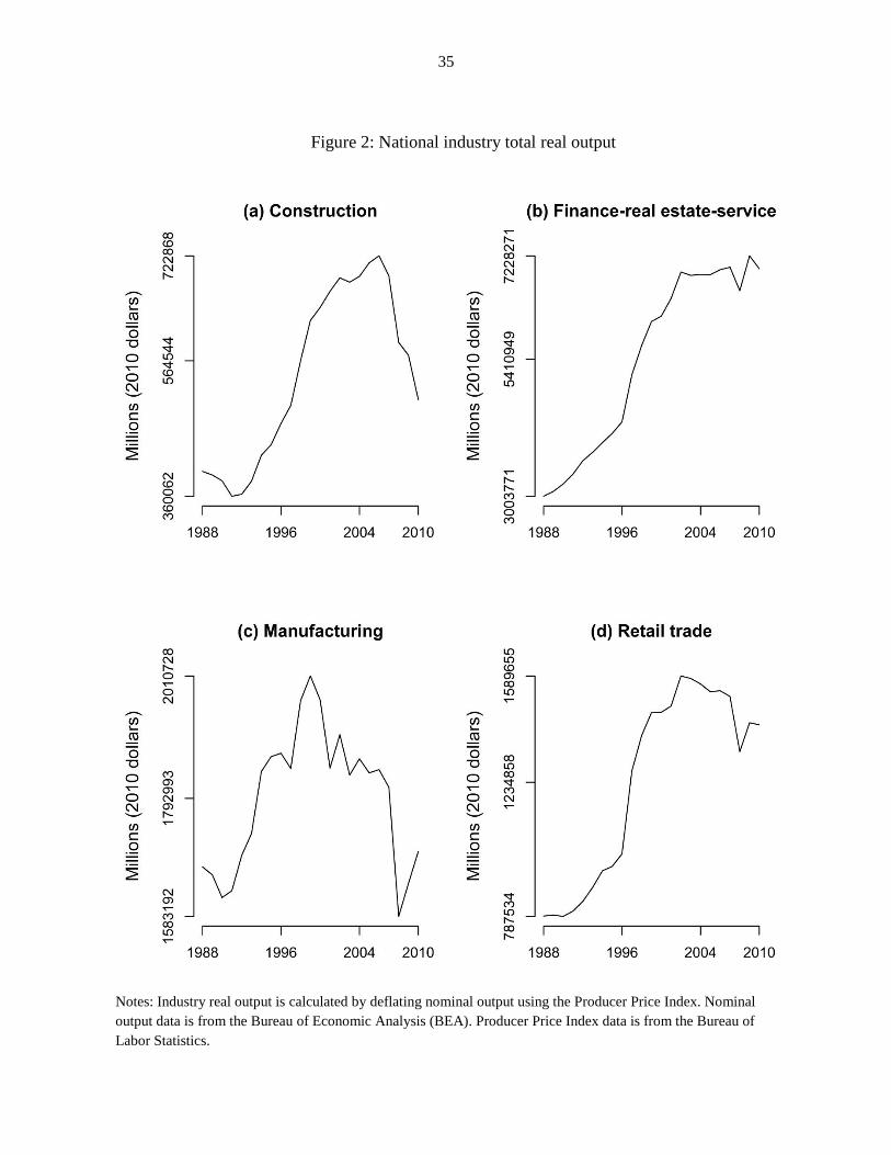
manufacturing sector. During the same time period, real output of the construction,
finance/insurance/real estate/service, manufacturing, and retail trade industries grew by 27
percent, 131 percent, 1 percent, and 79 percent, respectively. Figures 1 and 2 graph the evolution
of total national employment and average national real output in our sample.
The national average real wage rates ($/hour) in 1988 in the construction,
finance/insurance/real estate/service, manufacturing, and retail trade industries were 20, 19, 25,
and 10 respectively. In 2010, they stood at 21, 26, 24, and 10 respectively. Therefore, in the
period 1988-2010 employees in the construction and finance/insurance/real estate/service saw
modest growth in real wage rates, employees in manufacturing and retail trade actually witnessed
a decline in their real wage rates. A major reason for this is the great recession that hit the U.S. in
2008. Figure 3 plots the national annual average values of real wage rates for the four industries.
Following Blanchard and Katz (1992) we calculate two measures which can shift the labor
demand curve by affecting industry-county output. The first measure described in equation (3)
predicts output change for an industry-county, based on national output trends—it is called
Bartik’s IV, following Bartik (1991) who popularized its use as an instrument. In equation (3),
𝑌𝑖(−𝑐)𝑡 is the national output of industry 𝑖 less the industry output in county 𝑐. Bartik’s IV is
therefore the weighted average of changes in national industry outputs where the weights are
industry-county employment shares
𝐵𝑎𝑟𝑡𝑖𝑘_𝐼𝑉𝑐𝑡 =∑ 𝐸𝑚𝑝𝑙𝑜𝑦𝑒𝑒𝑠𝑖𝑐𝑡[ln(𝑌𝑖(−𝑐)𝑡)−ln(𝑌𝑖(−𝑐)𝑡−1)]𝑖
∑ 𝐸𝑚𝑝𝑙𝑜𝑦𝑒𝑒𝑠𝑖 𝑖𝑐𝑡
. (3)
10
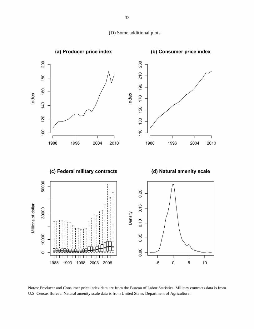
The second measure is dollar amounts in federal defense contracts received by each state in
the period 1988-2010. Data on federal defense contracts from the U.S. Census Bureau are not
available for every year, so the missing years were imputed using a linear interpolation method.
In Appendix (D) plot (c) we show a Box-plot for the federal defense contract.
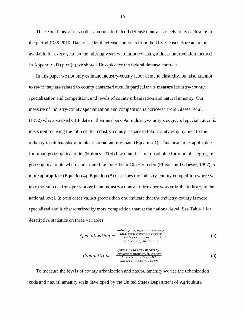
In this paper we not only estimate industry-county labor demand elasticity, but also attempt
to see if they are related to county characteristics. In particular we measure industry-county
specialization and competition, and levels of county urbanization and natural amenity. Our
measure of industry-county specialization and competition is borrowed from Glaeser et al.
(1992) who also used CBP data in their analysis. An industry-county’s degree of specialization is
measured by using the ratio of the industry-county’s share in total county employment to the
industry’s national share in total national employment (Equation 4). This measure is applicable
for broad geographical units (Holmes, 2004) like counties, but unsuitable for more disaggregate
geographical units where a measure like the Ellison-Glaeser index (Ellison and Glaeser, 1997) is
more appropriate (Equation 4). Equation (5) describes the industry-county competition where we
take the ratio of firms per worker in an industry-county to firms per worker in the industry at the
national level. In both cases values greater than one indicate that the industry-county is more
specialized and is characterized by more competition than at the national level. See Table 1 for
descriptive statistics on these variables.
𝑆𝑝𝑒𝑐𝑖𝑎𝑙𝑖𝑧𝑎𝑡𝑖𝑜𝑛 =
𝑖𝑛𝑑𝑢𝑠𝑡𝑟𝑦 𝑒𝑚𝑝𝑙𝑜𝑦𝑚𝑒𝑛𝑡 𝑖𝑛 𝑐𝑜𝑢𝑛𝑡𝑦
𝑡𝑜𝑡𝑎𝑙 𝑒𝑚𝑝𝑙𝑜𝑦𝑚𝑒𝑛𝑡 𝑖𝑛 𝑐𝑜𝑢𝑛𝑡𝑦𝑖𝑛𝑑𝑢𝑠𝑡𝑟𝑦 𝑒𝑚𝑝𝑙𝑜𝑦𝑚𝑒𝑛𝑡 𝑖𝑛 𝑈𝑆
𝑡𝑜𝑡𝑎𝑙 𝑒𝑚𝑝𝑙𝑜𝑦𝑚𝑒𝑛𝑡 𝑖𝑛 𝑈𝑆
. (4)
𝐶𝑜𝑚𝑝𝑒𝑡𝑖𝑡𝑖𝑜𝑛 =
𝑓𝑖𝑟𝑚𝑠 𝑖𝑛 𝑖𝑛𝑑𝑢𝑠𝑡𝑟𝑦 𝑖𝑛 𝑐𝑜𝑢𝑛𝑡𝑦
𝑤𝑜𝑟𝑘𝑒𝑟𝑠 𝑖𝑛 𝑖𝑛𝑑𝑢𝑠𝑡𝑟𝑦 𝑖𝑛 𝑐𝑜𝑢𝑛𝑡𝑦𝑓𝑖𝑟𝑚𝑠 𝑖𝑛 𝑖𝑛𝑑𝑢𝑠𝑡𝑟𝑦 𝑖𝑛 𝑈𝑆
𝑤𝑜𝑟𝑘𝑒𝑟𝑠 𝑖𝑛 𝑖𝑛𝑑𝑢𝑠𝑡𝑟𝑦 𝑖𝑛 𝑈𝑆
. (5)
To measure the levels of county urbanization and natural amenity we use the urbanization
code and natural amenity scale developed by the United States Department of Agriculture

11
(USDA)12. Based on this urbanization code we classify counties into three groups: metro
counties, non-metro counties that are urban and non-metro counties that are rural. In Appendix
(D) plot (d) we show a density plot for the natural amenity scale.
In this paper we also investigate the effect of government policies on industry-county labor
demand elasticity. In particular, we test if the presence of pro-business policies raises or lowers
labor demand elasticity. We classify states as pro-business if they have implemented a right-to-
work law, since Holmes (1998) claims that such states also tend to have a host of other pro-
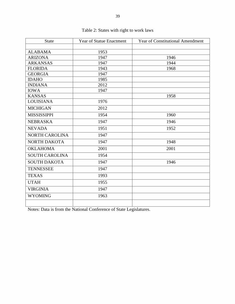
business policies. Table 2 lists the states that have adopted the right-to-work law along with the
year of adoption13.
If a union is certified at a place of work, then an employee might be required to join the
union or pay membership dues. This practice deals with the free rider problem where a worker
does not pay the cost of negotiation (membership fee, wage loss during the negotiation period if
a strike is called), but enjoys the benefits made possible by negotiations between management
and union. A right to work law removes the requirement of being a union member in order to
gain employment, or paying membership fees even if the non-union member worker will enjoy
the benefits arising from the union’s negotiations with the management (Leap, 1995). The right-
to-work law therefore can be viewed as pro-business since it weakens the power of unions and
strengthen employers’ position in bargaining.
3. Wage elasticity of labor demand: theory and estimation
12We would like to thank a referee for pointing us to this data source. 13Texas and Oklahoma implemented the right-to-work law in 1993 and 2001 respectively, which
straddle our study period, and Indiana and Michigan implemented them in 2012, which falls
outside our study period, we assume for our empirical analysis that these states are pro-business.
This is because, the eventual implementation of this law in these states signify the presence of
other pro-business policies (1998).
12
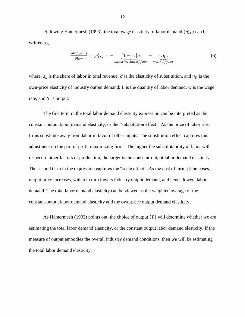
Following Hamermesh (1993), the total wage elasticity of labor demand (𝜂𝐿𝐿′ ) can be
written as,
𝛿𝑙𝑛𝐿(𝑤,𝑌)
𝛿𝑙𝑛𝑤= (𝜂𝐿𝐿
′ ) = − [1 − 𝑠𝐿]𝜎⏟ 𝑠𝑢𝑏𝑠𝑡𝑖𝑡𝑢𝑡𝑖𝑜𝑛 𝑒𝑓𝑓𝑒𝑐𝑡
− 𝑠𝐿𝜂𝐷⏟𝑠𝑐𝑎𝑙𝑒 𝑒𝑓𝑓𝑒𝑐𝑡
, (6)
where, 𝑠𝐿 is the share of labor in total revenue, 𝜎 is the elasticity of substitution, and 𝜂𝐷 is the
own-price elasticity of industry output demand; L is the quantity of labor demand, w is the wage
rate, and Y is output.
The first term in the total labor demand elasticity expression can be interpreted as the
constant-output labor demand elasticity, or the “substitution effect”. As the price of labor rises,
firms substitute away from labor in favor of other inputs. The substitution effect captures this
adjustment on the part of profit maximizing firms. The higher the substitutability of labor with
respect to other factors of production, the larger is the constant-output labor demand elasticity.
The second term in the expression captures the “scale effect”. As the cost of hiring labor rises,
output price increases, which in turn lowers industry output demand, and hence lowers labor
demand. The total labor demand elasticity can be viewed as the weighted average of the
constant-output labor demand elasticity and the own-price output demand elasticity.
As Hamermesh (1993) points out, the choice of output (𝑌) will determine whether we are
estimating the total labor demand elasticity, or the constant output labor demand elasticity. If the
measure of output embodies the overall industry demand conditions, then we will be estimating
the total labor demand elasticity.
13
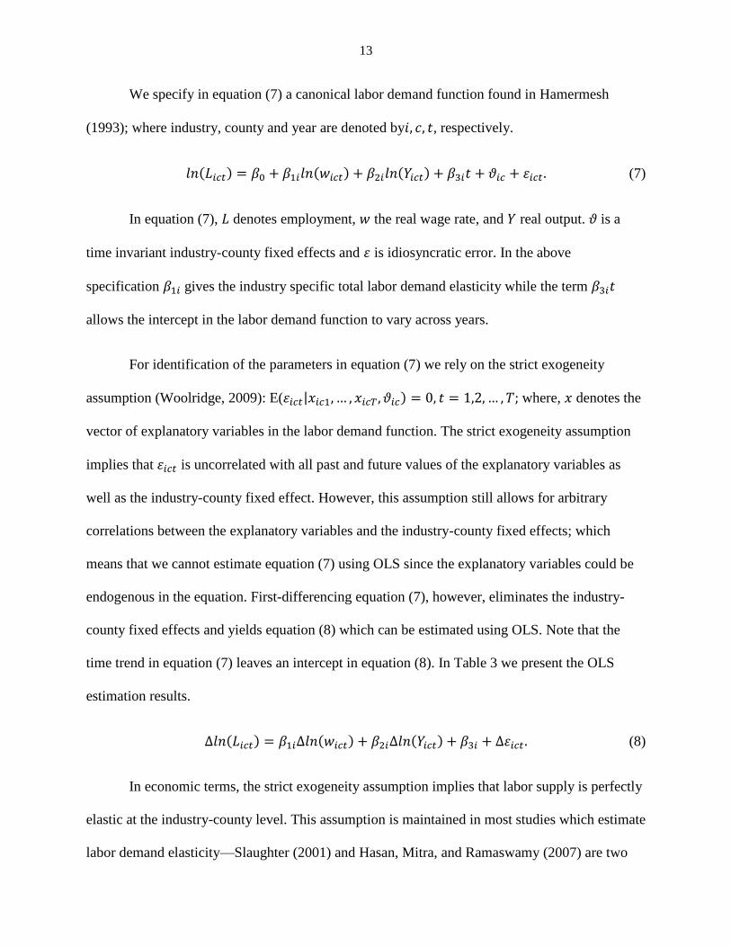
We specify in equation (7) a canonical labor demand function found in Hamermesh
(1993); where industry, county and year are denoted by𝑖, 𝑐, 𝑡, respectively.
𝑙𝑛(𝐿𝑖𝑐𝑡) = 𝛽0 + 𝛽1𝑖𝑙𝑛(𝑤𝑖𝑐𝑡) + 𝛽2𝑖𝑙𝑛(𝑌𝑖𝑐𝑡) + 𝛽3𝑖𝑡 + 𝜗𝑖𝑐 + 휀𝑖𝑐𝑡. (7)
In equation (7), 𝐿 denotes employment, 𝑤 the real wage rate, and 𝑌 real output. 𝜗 is a
time invariant industry-county fixed effects and 휀 is idiosyncratic error. In the above
specification 𝛽1𝑖 gives the industry specific total labor demand elasticity while the term 𝛽3𝑖𝑡
allows the intercept in the labor demand function to vary across years.
For identification of the parameters in equation (7) we rely on the strict exogeneity
assumption (Woolridge, 2009): E(휀𝑖𝑐𝑡|𝑥𝑖𝑐1, … , 𝑥𝑖𝑐𝑇 , 𝜗𝑖𝑐) = 0, 𝑡 = 1,2, … , 𝑇; where, 𝑥 denotes the
vector of explanatory variables in the labor demand function. The strict exogeneity assumption
implies that 휀𝑖𝑐𝑡 is uncorrelated with all past and future values of the explanatory variables as
well as the industry-county fixed effect. However, this assumption still allows for arbitrary
correlations between the explanatory variables and the industry-county fixed effects; which
means that we cannot estimate equation (7) using OLS since the explanatory variables could be
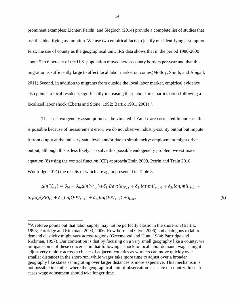
endogenous in the equation. First-differencing equation (7), however, eliminates the industry-
county fixed effects and yields equation (8) which can be estimated using OLS. Note that the
time trend in equation (7) leaves an intercept in equation (8). In Table 3 we present the OLS
estimation results.
Δ𝑙𝑛(𝐿𝑖𝑐𝑡) = 𝛽1𝑖Δ𝑙𝑛(𝑤𝑖𝑐𝑡) + 𝛽2𝑖Δ𝑙𝑛(𝑌𝑖𝑐𝑡) + 𝛽3𝑖 + Δ휀𝑖𝑐𝑡. (8)
In economic terms, the strict exogeneity assumption implies that labor supply is perfectly
elastic at the industry-county level. This assumption is maintained in most studies which estimate
labor demand elasticity—Slaughter (2001) and Hasan, Mitra, and Ramaswamy (2007) are two
14
prominent examples; Lichter, Peichi, and Siegloch (2014) provide a complete list of studies that
use this identifying assumption. We use two empirical facts to justify our identifying assumption.
First, the use of county as the geographical unit: IRS data shows that in the period 1980-2000
about 5 to 6 percent of the U.S. population moved across county borders per year and that this
migration is sufficiently large to affect local labor market outcomes(Molloy, Smith, and Abigail,
2011).Second, in addition to migrants from outside the local labor market, empirical evidence
also points to local residents significantly increasing their labor force participation following a
localized labor shock (Eberts and Stone, 1992; Bartik 1991, 2001)14.
The strict exogeneity assumption can be violated if 𝑌and 휀 are correlated.In our case this
is possible because of measurement error: we do not observe industry-county output but impute
it from output at the industry-state level and/or due to simultaneity: employment might drive
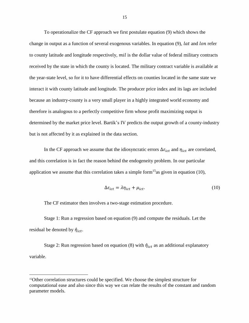
output, although this is less likely. To solve this possible endogeneity problem we estimate
equation (8) using the control function (CF) approach(Train 2009, Petrin and Train 2010,
Woolridge 2014) the results of which are again presented in Table 3.
Δ𝑙𝑛(𝑌𝑖𝑐𝑡) = 𝛿0𝑖 + 𝛿0𝑖Δ𝑙𝑛(𝑤𝑖𝑐𝑡)+𝛿1𝑖𝐵𝑎𝑟𝑡𝑖𝑘𝐼𝑉𝑐𝑡 + 𝛿2𝑖𝑙𝑎𝑡𝑖𝑚𝑖𝑙𝑠(𝑐)𝑡 + 𝛿3𝑖𝑙𝑜𝑛𝑖𝑚𝑖𝑙𝑠(𝑐)𝑡 +
𝛿4𝑖𝑙𝑜𝑔(𝑃𝑃𝐼𝑡) + 𝛿5𝑖𝑙𝑜𝑔(𝑃𝑃𝐼𝑡−1) + 𝛿6𝑖𝑙𝑜𝑔(𝑃𝑃𝐼𝑡−2) + 𝜂𝑖𝑐𝑡 . (9)
14A referee points out that labor supply may not be perfectly elastic in the short-run (Bartik,
1993; Partridge and Rickman, 2003, 2006; Rowthorn and Glyn, 2006) and analogous to labor
demand elasticity might vary across regions (Greenwood and Hunt, 1984; Partridge and
Rickman, 1997). Our contention is that by focusing on a very small geography like a county, we
mitigate some of these concerns, in that following a shock to local labor demand, wages might
adjust very rapidly across a cluster of adjacent counties as workers can move quickly over
smaller distances in the short-run, while wages take more time to adjust over a broader
geography like states as migrating over larger distances is more expensive. This mechanism is
not possible in studies where the geographical unit of observation is a state or country. In such
cases wage adjustment should take longer time.
15
To operationalize the CF approach we first postulate equation (9) which shows the
change in output as a function of several exogenous variables. In equation (9), 𝑙𝑎𝑡 and 𝑙𝑜𝑛 refer
to county latitude and longitude respectively, 𝑚𝑖𝑙 is the dollar value of federal military contracts
received by the state in which the county is located. The military contract variable is available at
the year-state level, so for it to have differential effects on counties located in the same state we
interact it with county latitude and longitude. The producer price index and its lags are included
because an industry-county is a very small player in a highly integrated world economy and
therefore is analogous to a perfectly competitive firm whose profit maximizing output is
determined by the market price level. Bartik’s IV predicts the output growth of a county-industry
but is not affected by it as explained in the data section.
In the CF approach we assume that the idiosyncratic errors Δ휀𝑖𝑐𝑡 and 𝜂𝑖𝑐𝑡 are correlated,
and this correlation is in fact the reason behind the endogeneity problem. In our particular
application we assume that this correlation takes a simple form15as given in equation (10),
Δ휀𝑖𝑐𝑡 = 𝜆𝜂𝑖𝑐𝑡 + 𝜇𝑖𝑐𝑡. (10)
The CF estimator then involves a two-stage estimation procedure.
Stage 1: Run a regression based on equation (9) and compute the residuals. Let the
residual be denoted by �̂�𝑖𝑐𝑡.
Stage 2: Run regression based on equation (8) with �̂�𝑖𝑐𝑡 as an additional explanatory
variable.
15Other correlation structures could be specified. We choose the simplest structure for
computational ease and also since this way we can relate the results of the constant and random
parameter models.
16
The resulting estimator is the CF estimator and it provides consistent estimates of the
parameters in equation (7). This particular CF estimator is equivalent to a 2SLS estimator
(Hausman, 1978).
In the labor demand equation presented in the previous section the coefficient of log
wage is a constant: there is no variation in the wage elasticity of labor demand across counties
and/or over time. In the constant parameter linear panel data framework discussed earlier we
cannot estimate a 𝛽1𝑖for each county-year combination, otherwise, the number of parameters to
estimate will be greater than the number of observations in the data. To incorporate regional
variation in labor demand elasticity, we can estimate a 𝛽1𝑖 for each county. The problem with
this approach is that there is no guarantee that all the 𝛽1𝑖 will have the correct sign and the
sample sizes will be significantly smaller making the estimates unreliable.
An alternative approach to incorporate spatial heterogeneity in labor demand elasticity
would be to interact log wage with some variable which we believe affects labor demand
elasticity and which itself varies across counties. However, there are two drawbacks with this
approach. One, since multiple factors influence labor demand elasticity, the result will crucially
depend on the choice of the interaction variables. Two, theory provides little guidance as to what
these interaction variables should be.
Borrowing from ideas in the random parameter discrete choice literature (Train, 2009) we
use a more robust approach to incorporate spatial heterogeneity in labor demand elasticity: we
assume that the parameter 𝛽1𝑖 is a random variable16. In which case we cannot estimate 𝛽1𝑖, but
we can estimate the parameters which describe the distribution of 𝛽1𝑖 in the population of
16See Hsiao and Pesaran (2004) for other approaches in specification and estimation of random
parameter panel data models.
17
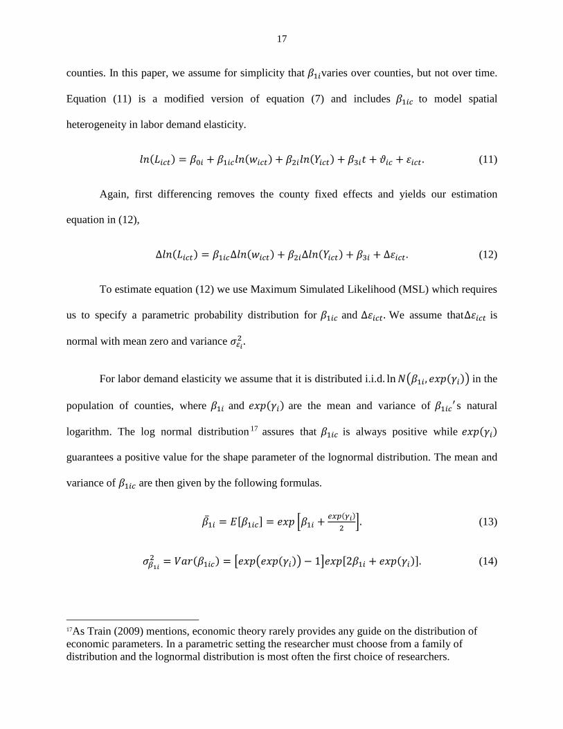
counties. In this paper, we assume for simplicity that 𝛽1𝑖varies over counties, but not over time.
Equation (11) is a modified version of equation (7) and includes 𝛽1𝑖𝑐 to model spatial
heterogeneity in labor demand elasticity.
𝑙𝑛(𝐿𝑖𝑐𝑡) = 𝛽0𝑖 + 𝛽1𝑖𝑐𝑙𝑛(𝑤𝑖𝑐𝑡) + 𝛽2𝑖𝑙𝑛(𝑌𝑖𝑐𝑡) + 𝛽3𝑖𝑡 + 𝜗𝑖𝑐 + 휀𝑖𝑐𝑡. (11)
Again, first differencing removes the county fixed effects and yields our estimation
equation in (12),
Δ𝑙𝑛(𝐿𝑖𝑐𝑡) = 𝛽1𝑖𝑐Δ𝑙𝑛(𝑤𝑖𝑐𝑡) + 𝛽2𝑖Δ𝑙𝑛(𝑌𝑖𝑐𝑡) + 𝛽3𝑖 + Δ휀𝑖𝑐𝑡. (12)
To estimate equation (12) we use Maximum Simulated Likelihood (MSL) which requires
us to specify a parametric probability distribution for 𝛽1𝑖𝑐 and Δ휀𝑖𝑐𝑡. We assume thatΔ휀𝑖𝑐𝑡 is
normal with mean zero and variance 𝜎𝑖
2 .
For labor demand elasticity we assume that it is distributed i.i.d. ln𝑁(𝛽1𝑖, 𝑒𝑥𝑝(𝛾𝑖)) in the
population of counties, where 𝛽1𝑖 and 𝑒𝑥𝑝(𝛾𝑖) are the mean and variance of 𝛽1𝑖𝑐′ s natural
logarithm. The log normal distribution 17 assures that 𝛽1𝑖𝑐 is always positive while 𝑒𝑥𝑝(𝛾𝑖)
guarantees a positive value for the shape parameter of the lognormal distribution. The mean and
variance of 𝛽1𝑖𝑐 are then given by the following formulas.
�̅�1𝑖 = 𝐸[𝛽1𝑖𝑐] = 𝑒𝑥𝑝 [𝛽1𝑖 +𝑒𝑥𝑝(𝛾𝑖)
2]. (13)
𝜎𝛽1𝑖2 = 𝑉𝑎𝑟(𝛽1𝑖𝑐) = [𝑒𝑥𝑝(𝑒𝑥𝑝(𝛾𝑖)) − 1]𝑒𝑥𝑝[2𝛽1𝑖 + 𝑒𝑥𝑝(𝛾𝑖)]. (14)
17As Train (2009) mentions, economic theory rarely provides any guide on the distribution of
economic parameters. In a parametric setting the researcher must choose from a family of
distribution and the lognormal distribution is most often the first choice of researchers.
18
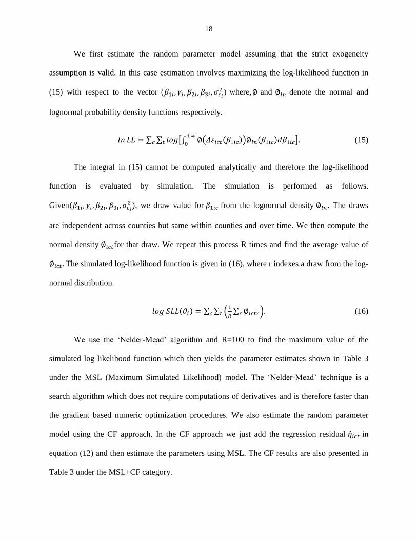
We first estimate the random parameter model assuming that the strict exogeneity
assumption is valid. In this case estimation involves maximizing the log-likelihood function in
(15) with respect to the vector (𝛽1𝑖, 𝛾𝑖, 𝛽2𝑖, 𝛽3𝑖, 𝜎 𝑖
2) where,∅ and ∅𝑙𝑛 denote the normal and
lognormal probability density functions respectively.
𝑙𝑛 𝐿𝐿 = ∑ ∑ 𝑙𝑜𝑔[∫ ∅(𝛥휀𝑖𝑐𝑡(𝛽1𝑖𝑐))∅𝑙𝑛(𝛽1𝑖𝑐)𝑑𝛽1𝑖𝑐+∞
0].𝑡𝑐 (15)
The integral in (15) cannot be computed analytically and therefore the log-likelihood
function is evaluated by simulation. The simulation is performed as follows.
Given(𝛽1𝑖, 𝛾𝑖, 𝛽2𝑖, 𝛽3𝑖, 𝜎 𝑖
2), we draw value for 𝛽1𝑖𝑐 from the lognormal density ∅𝑙𝑛. The draws
are independent across counties but same within counties and over time. We then compute the
normal density ∅𝑖𝑐𝑡for that draw. We repeat this process R times and find the average value of
∅𝑖𝑐𝑡. The simulated log-likelihood function is given in (16), where r indexes a draw from the log-
normal distribution.
𝑙𝑜𝑔 𝑆𝐿𝐿(𝜃𝑖) = ∑ ∑ (1
𝑅∑ ∅𝑖𝑐𝑡𝑟𝑟 )𝑡𝑐 . (16)
We use the ‘Nelder-Mead’ algorithm and R=100 to find the maximum value of the
simulated log likelihood function which then yields the parameter estimates shown in Table 3
under the MSL (Maximum Simulated Likelihood) model. The ‘Nelder-Mead’ technique is a
search algorithm which does not require computations of derivatives and is therefore faster than
the gradient based numeric optimization procedures. We also estimate the random parameter
model using the CF approach. In the CF approach we just add the regression residual �̂�𝑖𝑐𝑡 in
equation (12) and then estimate the parameters using MSL. The CF results are also presented in
Table 3 under the MSL+CF category.
19
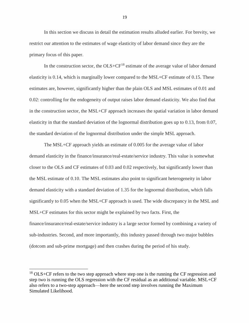
In this section we discuss in detail the estimation results alluded earlier. For brevity, we
restrict our attention to the estimates of wage elasticity of labor demand since they are the
primary focus of this paper.
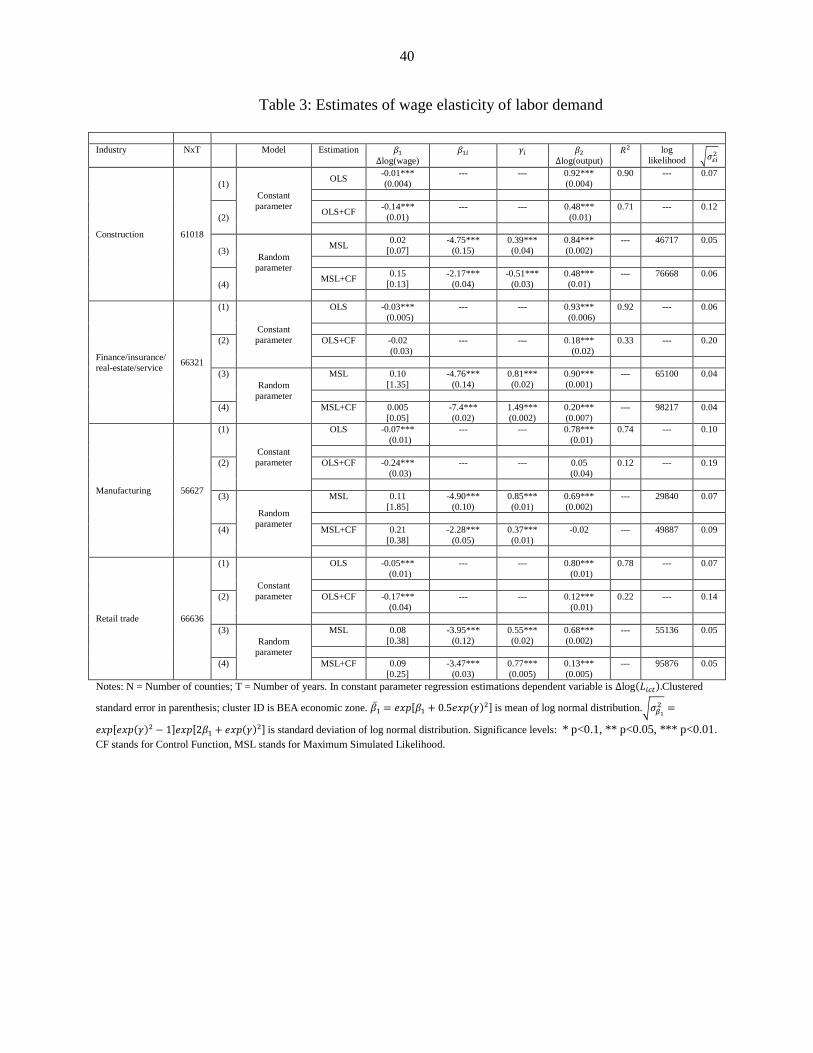
In the construction sector, the OLS+CF18 estimate of the average value of labor demand
elasticity is 0.14, which is marginally lower compared to the MSL+CF estimate of 0.15. These
estimates are, however, significantly higher than the plain OLS and MSL estimates of 0.01 and
0.02: controlling for the endogeneity of output raises labor demand elasticity. We also find that
in the construction sector, the MSL+CF approach increases the spatial variation in labor demand
elasticity in that the standard deviation of the lognormal distribution goes up to 0.13, from 0.07,
the standard deviation of the lognormal distribution under the simple MSL approach.
The MSL+CF approach yields an estimate of 0.005 for the average value of labor
demand elasticity in the finance/insurance/real-estate/service industry. This value is somewhat
closer to the OLS and CF estimates of 0.03 and 0.02 respectively, but significantly lower than
the MSL estimate of 0.10. The MSL estimates also point to significant heterogeneity in labor
demand elasticity with a standard deviation of 1.35 for the lognormal distribution, which falls
significantly to 0.05 when the MSL+CF approach is used. The wide discrepancy in the MSL and
MSL+CF estimates for this sector might be explained by two facts. First, the
finance/insurance/real-estate/service industry is a large sector formed by combining a variety of
sub-industries. Second, and more importantly, this industry passed through two major bubbles
(dotcom and sub-prime mortgage) and then crashes during the period of his study.
18 OLS+CF refers to the two step approach where step one is the running the CF regression and
step two is running the OLS regression with the CF residual as an additional variable. MSL+CF
also refers to a two-step approach—here the second step involves running the Maximum
Simulated Likelihood.
20
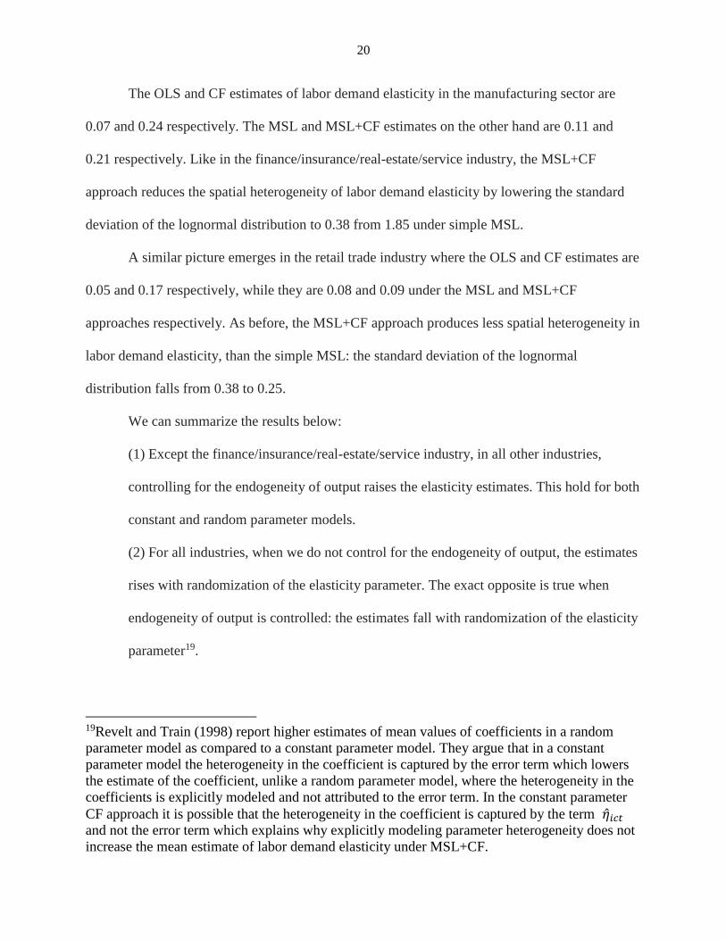
The OLS and CF estimates of labor demand elasticity in the manufacturing sector are
0.07 and 0.24 respectively. The MSL and MSL+CF estimates on the other hand are 0.11 and
0.21 respectively. Like in the finance/insurance/real-estate/service industry, the MSL+CF
approach reduces the spatial heterogeneity of labor demand elasticity by lowering the standard
deviation of the lognormal distribution to 0.38 from 1.85 under simple MSL.
A similar picture emerges in the retail trade industry where the OLS and CF estimates are
0.05 and 0.17 respectively, while they are 0.08 and 0.09 under the MSL and MSL+CF
approaches respectively. As before, the MSL+CF approach produces less spatial heterogeneity in
labor demand elasticity, than the simple MSL: the standard deviation of the lognormal
distribution falls from 0.38 to 0.25.
We can summarize the results below:
(1) Except the finance/insurance/real-estate/service industry, in all other industries,
controlling for the endogeneity of output raises the elasticity estimates. This hold for both
constant and random parameter models.
(2) For all industries, when we do not control for the endogeneity of output, the estimates
rises with randomization of the elasticity parameter. The exact opposite is true when
endogeneity of output is controlled: the estimates fall with randomization of the elasticity
parameter19.
19Revelt and Train (1998) report higher estimates of mean values of coefficients in a random
parameter model as compared to a constant parameter model. They argue that in a constant
parameter model the heterogeneity in the coefficient is captured by the error term which lowers
the estimate of the coefficient, unlike a random parameter model, where the heterogeneity in the
coefficients is explicitly modeled and not attributed to the error term. In the constant parameter
CF approach it is possible that the heterogeneity in the coefficient is captured by the term �̂�𝑖𝑐𝑡 and not the error term which explains why explicitly modeling parameter heterogeneity does not
increase the mean estimate of labor demand elasticity under MSL+CF.

21
(3) In the random parameter model the CF approach estimates less spatial heterogeneity
in labor demand elasticity as compared to the simple MSL approach. This result,
however, does not hold for the construction sector.
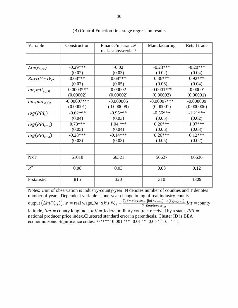
Before we move on, it is important to mention briefly the results (Appendix B) of the
first-stage regression in the CF approach. We find that all the regressions are highly significant,
as pointed out by the very high values of the F-statistics, plus, most of the coefficients in the
regression are also individually highly statistically significant20. Exceptions are the military
contract variables which are not significant in the finance/insurance/real-estate/service and retail
trade industries. This is expected as most of the benefits of such contract likely fall on the other
two sectors: construction and manufacturing, for which they are highly statistically significant.
4. Regional variations in labor demand elasticity and its determinants
In the previous section we presented estimates for the mean and standard deviation of the
lognormal distributions which describe the spatial variations in labor demand elasticity for four
industries in the U.S. These distributions then allows us to calculate average labor demand
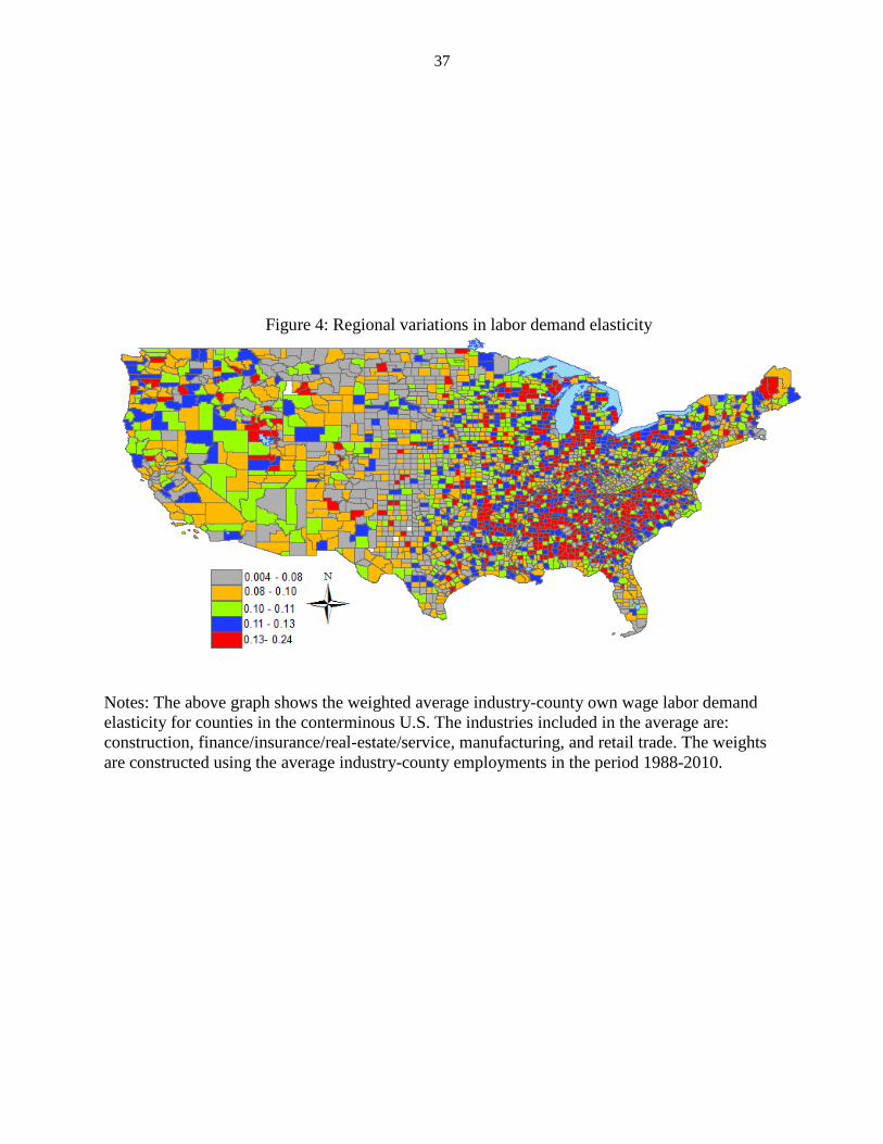
elasticity for each industry-county (see Appendix C)--in Figure 4 we map the weighted averages
of the four industry-county elasticity using industry-county employment shares as weights. In
this section we attempt to relate these variations in labor demand elasticity to differences in other
county characteristics. This analysis will reveal if the variations in labor demand elasticity is
random or is systematically related to other county characteristics.
In Table 4 we present regression results which show some clear trends in the spatial
variations in labor demand elasticity. We find that counties with higher levels of natural amenity
have higher labor demand elasticity. Industry-county competition has a negative relationship
20This result alleviates concerns of weak instruments (Stock and Yogo, 2005).

22
with labor demand elasticity. Industry-county specialization also has a negative relationship, as
long as we control for industry-county competition, otherwise it has a statistically insignificant
positive relationship. The level of urbanization as measured by the dummy variables has a
positive relationship with labor demand elasticity: more urbanized counties have higher labor
demand elasticity. Finally, counties with right-to-work laws have lower labor demand elasticity--
this relationship is not statistically significant. This result, however, goes contrary to economic
sense which says that right-to-work laws should make firms more flexible to hire/fire workers
and therefore push up labor demand elasticity. Given that a lot of government policies are at play
at the county level, we need a more sophisticated approach to elicit the relationship between the
right-to-work law and labor demand elasticity (Holmes, 1998). The next section describes just
such an approach.
What explains the relationships in Table 4? One interpretation is that some of the
relationships in Table 4 captures the biases in our elasticity estimates because of our assumption
of perfectly elastic labor supply. For example, a county with higher level of natural amenity
might have a better chance of attracting workers than a comparable county with lower natural
amenity level, thereby implying different supply elasticity for the two counties. Similarly,
metropolitan and urban counties might be able to attract more workers given that they offer
better consumption opportunities to its inhabitants than rural counties. However, given the very
small magnitudes of the effects in Table 4, we can be reasonably confident that the biases--if
they exist--are very small.
The effect of industry-specialization and industry-competition on labor demand elasticity
is more difficult to explain since economic theory does not provide any guide as to what these
relationships should be. One possible explanation for industry-county competition is that more
23
firms in an industry increases firms' search and matching costs of hiring/firing workers and so
they become less responsive to wage shocks. The effect of industry-county specialization is more
ambiguous and difficult to explain.
To find the effect of pro-business policies on labor demand elasticity we follow the
research design laid out in Holmes (1998): we look for abrupt changes in labor demand elasticity
at borders which divide states with and without right-to-work laws. At state borders factors that
affect labor demand elasticity are approximately same on both sides of the border and so the
difference in labor demand elasticity on two sides can only be attributed to government policy.
Equation (17) describes the regression equation that is used to test this hypothesis,
�̌�1𝑖𝑐 = 𝜃𝑟𝑐 + 𝛼(𝑥𝑐) + 𝛿𝑦𝑐 + 𝜖𝑖𝑐. (17)
In equation (17), 𝜃𝑟𝑐 is a shift parameter which equals 𝜃 if the county belongs to a right-
to-work state, zero otherwise. Following Holmes (1998) we consider two border segments21.
Segment 1 begins at the western end of the Oklahoma-Texas border and ends where the
Maryland-Virginia border meets the Atlantic Ocean. Segment 2 begins where the Minnesota-
North Dakota border intersects the boundary with Canada and it ends at the western end of the
Oklahoma-Kansas border. Segment 1 is 2386 miles long while segment 2 has a length of 1891
miles. The variable 𝑥𝑐 is used to mark points every one-mile along these two-border segments.
For example, 𝑥𝑐 = 0 and 𝑥𝑐 = 2386 are at the start and end of border segment 1 respectively. In
equation (17), 𝑥𝑐 is the mile marker closest to the centroid of the county polygon and 𝑦𝑐
measures the distance between them—𝑦𝑐 is negative if the county is in a right to work state and
positive otherwise. 𝛼(𝑥𝑐) represents a general continuous function of 𝑥𝑐 . Following Holmes
(1998) we restrict ourselves to counties within 100 miles of the two border segment. Holmes
21See Holmes (1998) for the map which outlines the two border segments.
24
(1998) justifies a nonlinear relationship between the dependent variable and 𝑥𝑐 since movement
along 𝑥 covers a large distance while movement along 𝑦 is small—100 miles on each side of the
border, and so a linear relationship between the dependent variable and 𝑦 is reasonable.
In Table 5 we show the OLS estimates of 𝜃𝑟𝑐 for two different specifications. In both
specifications we use a fourth-degree polynomial to approximate 𝛼(𝑥𝑐). In specification 1, 𝛿 is
same for both border segments while in specification 2 they are different. The positive estimate
of 𝜃 under both specifications supports our hypothesis that labor demand elasticity is higher in
states with right-to-work laws or more precisely states which are more pro-business22.
5. Conclusion
In this study we find evidence of spatial variations in labor demand elasticity and provide
point estimates for them at the industry-county level. We also find that the spatial variations in
elasticity are not the result of some random assignment but are systematically related to certain
spatial features of the U.S. economy and urban landscape. In this section we discuss some future
research ideas that could extend and improve this study.
One obvious extension of this study will be to relax the assumption of perfectly elastic
labor supply. This can be done either by finding a reliable instrument for wage or by explicitly
modeling labor supply and taking the simultaneous equations estimation approach. In the latter
approach labor supply can emerge from workers metropolitan residence location choice--which
can be modeled using random utility models. Such an approach will also allow the joint
estimation of the labor and land/housing markets since labor supply and housing demand are two
22As a robustness check we re-estimated the parameters in equation 17 after assigning Texas,
Oklahoma, Michigan, and Indiana as non-right-to-work states, since in these states the laws were
implemented either during or after our study period. This reassignment does not change the
results reported in Table 5 significantly.

25
sides of the same coin, at least at a metropolitan area level. Another direction of research should
be to explore the theoretical underpinnings of the relationships between labor demand elasticity
and county characteristics, especially industry-county specialization and industry-county
competition. This will improve our understanding of the dynamics of local labor markets and
how they are related to the spatial organization of economic activity and urban structure.
26
6. References
Bartik, Timothy J. 1991. "Who benefits from state and local economic development policies?,"
Kalamazoo, MI: W.E. Upjohn Institute for Employment Research.
Bartik, Timothy J. 2002. "Evaluating the impacts of local economic development policies on
local economic outcomes: what has been done and what is doable?" Kalamazoo, MI: W.E.
Upjohn Institute for Employment Research.
Blanchard, Olivier Jean, and Lawrence F. Katz. 1992. "Regional evolutions," Brookings Papers
on Economic Activity, 1992(1), 1-75.
Brent, Richard. 1973. Algorithms for minimization without derivatives. Englewood Cliffs, New
Jersey: Prentice-Hall.
Brunsdon, Chris, A. Stewart Fotheringham, and Martin E. Charlton. 1996. "Geographically
weighted regression: a method for exploring spatial non-stationarity," Geographical Analysis,
28(4), 281-298.
Eberts, Randall, and Joe A. Stone. 1992. "Wage and employment adjustment in local labor
markets," Kalamazoo, MI: W.E. Upjohn Institute for Employment Research.
Ellison, Glenn, and Edward L. Glaeser. 1997. "Geographic concentration in U.S. manufacturing
industries: a dartboard approach," Journal of Political Economy, 105(5), 889-927.
Fingleton, Bernard, Harry Garretsen, and Ron Martin. 2012. "Recessionary shocks and regional
employment: evidence on the resilience of U.K. regions," Journal of Regional Science, 52(1),
109-133.
Glaeser, Edward L., Hedi D. Kallal, José A. Scheinkman, and Andrei Shleifer. 1992. "Growth in
cities," Journal of Political Economy, 100(6), 1126-1152.
Glaeser, Edward, and Joshua D. Gottlieb. 2009. "The wealth of cities: agglomeration economies
and spatial equilibrium in the United States," Journal of Economic Literature, 47 (4), 983-1028.
Hamermesh, Daniel S. 1993. Labor demand. Princeton, New Jersey: Princeton University Press.
Hasan, Rana, Devashish Mitra, and K.V. Ramaswamy. 2007. "Trade reforms, labor regulations,
and labour-demand elasticities: empirical evidence from India," The Review of Economics and
Statistics, 89(3), 466-481.
Hausman, J. A. 1978. "Specification tests in econometrics," Econometrica, 46(6), 1251-1271.
Holmes, Thomas J. 1998. "The evidence of state policies on the location of industry: evidence
from state borders," Journal of Political Economy, 106 (4), 667-705.
27
Holmes, Thomas J., and John J. Stevens. 2004. “Spatial distribution of economic activities in
North America,” in Handbook of Regional and Urban Economics, V. Henderson and J.F. Thisse
(eds.), Vol. 4, 2797-2843.
Hsiao, Cheng, and M. Hashem Pesaran. 2004. “Random coefficient panel data model,” IZA
Discussion Paper Series, No. 1236.
Isserman, Andrew M., and James Westervelt. 2006. "1.5 million missing numbers: overcoming
employment suppression in County Business Patterns data," International Regional Science
Review, 29(3), 311-335.
Katz, Lawrence F. 1996. “Wage subsidies for the disadvantaged,” NBER working paper 5679,
National Bureau of Economic Research.
Leap, Terry L. 1995. Collective bargaining and labor relations. Englewood Cliffs, New Jersey:
Prentice Hall.
Lichter, Andreas, Andreas Peichl, and Sebastian Siegloch. 2014. “The own-wage elasticity of
labor demand: a meta-regression analysis,” Discussion Paper, IZA.
McMillen, Daniel P. 2010. "Issues in spatial analysis." Journal of Regional Science, 50(1), 119-
141.
Molloy, Raven, Christopher L. Smith, and Abigail Wozniak. 2011. "Internal migration in the
United States," Journal of Economic Perspectives, 25(3), 173-196.
Moretti, Enrico. 2011. "Local labor markets," In Handbook of Labor Economics, David Card and
Orley Ashenfelter (eds.), Vol 4(B), 1237-1313.
Partridge, Mark D, and Dan S Rickman. 2006. "An SVAR model of fluctuations in U.S.
migration flows and state labor market dynamics," Southern Economic Journal, 72(4), 958-980.
Partridge, Mark D., and Dan S. Rickman. 2010. "Computable general equilibrium (CGE)
modelling for regional development analysis," Regional Studies, 44(10), 1311-1328.
Partridge, Mark D., and Dan S. Rickman. 1997. "The dispersion of U.S. State unemployment
rates: the role of market and non-market equilibrium factors," Regional Studies, 31(6), 593-606.
Partridge, Mark D., and Dan S. Rickman. 2003. "The waxing and waning of regional economies:
the chicken-egg question of jobs versus people," Journal of Urban Economics, 53(1), 76-97.
Petrin, Amil, and Kenneth Train. 2010. "A control function approach to endogeneity in consumer
choice models," Journal of Marketing Research, 47(1), 3-13.
Revelt, David, and Kenneth Train. 1998. "Mixed logit with repeated choices: households'
choices of appliance efficiency level," The Review of Economics and Statistics, 80(4), 647-657.
28
Roback, Jennifer. 1982. "Wages, rents, and the quality of life," Journal of Political Economy,
90(6), 1257-1278.
Rosen, Sherwin. 1979. "Wage-based indexes of urban quality of life,” In Current Issues in Urban
Economics, Miezkowski, and Straszheim (eds.), Baltimore, Maryland: John Hopkins University
Press.
Rowthorn, Robert, and Andrew Glyn. 2006. "Convergence and stability in U.S. employment
rates." The B.E. Journal of Macroeconomics, 6(1), 1-43.
Simon, Curtis. 2014. "Sectoral change and unemployment during the great recession in historical
perspective," Journal of Regional Science, 54(5), 828-855.
Slaughter, Matthew J. 2001. "International trade and labor-demand elasticities," Journal of
International Economics, 54(1), 27-56.
Stock, James H., and Motohiro Yogo. 2005. "Testing for weak instruments in linear IV
regression," In Identification and inference for econometric models: essays in honor of Thomas
Rothenberg, D.W.K. Andrews and James H. Stock (eds.). Cambridge, United Kingdom:
Cambridge University Press.
Train, Kenneth. 2009. Discrete choice methods with simulation. Cambridge, United Kingdom:
Cambridge University Press.
Wooldridge, Jeffrey M. 2014. "Quasi-maximum likelihood estimation and testing for nonlinear
models with endogenous explanatory variables," Journal of Econometrics, 182(1), 226-234.
Woolridge, Jeffrey. 2010. Econometric analysis of cross section and panel data. Cambridge,
Massachusetts: MIT press.

29
7. Appendix
(A) 1993 rural-urban continuum code (also known as the "Beale code")
Metro counties:
0 Central counties of metro areas of 1 million population or more
1 Fringe counties of metro areas of 1 million population or more
2 Counties in metro areas of 250,000 to 1 million population
3 Counties in metro areas of fewer than 250,000 population
Non-metro counties:
4 Urban population of 20,000 or more, adjacent to a metro area
5 Urban population of 20,000 or more, not adjacent to a metro area
6 Urban population of 2,500 to 19,999, adjacent to a metro area
7 Urban population of 2,500 to 19,999, not adjacent to a metro area
8 Completely rural or fewer than 2,500 urban population, adjacent to a
metro area
9 Completely rural or fewer than 2,500 urban population, not adjacent
to a metro area
Population is 1990.
Source: http://www.ers.usda.gov/briefing/rurality/ruralurbcon/.
30
(B) Control Function first-stage regression results
Variable Construction Finance/insurance/
real-estate/service/
Manufacturing Retail trade
Δ𝑙𝑛(𝑤𝑖𝑐𝑡) -0.29***
(0.02)
-0.02
(0.03)
-0.23***
(0.02)
-0.20***
(0.04)
𝐵𝑎𝑟𝑡𝑖𝑘′𝑠 𝐼𝑉𝑐𝑡 0.68***
(0.07)
0.68***
(0.05)
0.36***
(0.06)
0.92***
(0.04)
𝑙𝑎𝑡𝑐𝑚𝑖𝑙𝑠(𝑐)𝑡 -0.0003***
(0.00002)
0.00002
(0.00002)
-0.0001***
(0.00003)
-0.00001
(0.00001)
𝑙𝑜𝑛𝑐𝑚𝑖𝑙𝑠(𝑐)𝑡 -0.00007***
(0.00001)
-0.000005
(0.000009)
-0.00007***
(0.00001)
-0.000009
(0.000006)
𝑙𝑜𝑔(𝑃𝑃𝐼𝑡) -0.62***
(0.04)
-0.95***
(0.03)
-0.56***
(0.05)
-1.21***
(0.02)
𝑙𝑜𝑔(𝑃𝑃𝐼𝑡−1) 0.73***
(0.05)
1.04 ***
(0.04)
0.26***
(0.06)
1.07***
(0.03)
𝑙𝑜𝑔(𝑃𝑃𝐼𝑡−2) -0.28***
(0.03)
-0.14***
(0.03)
0.26***
(0.05)
0.12***
(0.02)
NxT 61018 66321 56627 66636
𝑅2 0.08 0.03 0.03 0.12
F-statistic 815 320 310 1309
Notes: Unit of observation is industry-county-year. N denotes number of counties and T denotes
number of years. Dependent variable is one-year change in log of real industry-county
output (Δ𝑙𝑛(𝑌𝑖𝑐𝑡)). 𝑤 = real wage,𝐵𝑎𝑟𝑡𝑖𝑘′𝑠 𝐼𝑉𝑐𝑡 =∑ 𝐸𝑚𝑝𝑙𝑜𝑦𝑒𝑒𝑠𝑖𝑐𝑡[ln(𝑌𝑖(−𝑐)𝑡)−ln(𝑌𝑖(−𝑐)𝑡−1)]𝑖
∑ 𝐸𝑚𝑝𝑙𝑜𝑦𝑒𝑒𝑠𝑖 𝑖𝑐𝑡
,𝑙𝑎𝑡 =county
latitude, 𝑙𝑜𝑛 = county longitude, 𝑚𝑖𝑙 = federal military contract received by a state, 𝑃𝑃𝐼 =
national producer price index.Clustered standard error in parenthesis. Cluster ID is BEA
economic zone. Significance codes: 0 ‘***’ 0.001 ‘**’ 0.01 ‘*’ 0.05 ‘.’ 0.1 ‘ ’ 1.
31
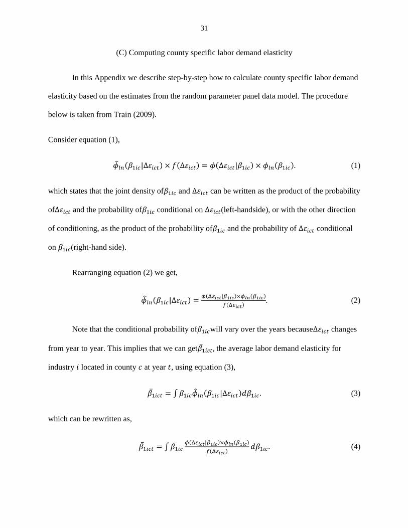
(C) Computing county specific labor demand elasticity
In this Appendix we describe step-by-step how to calculate county specific labor demand
elasticity based on the estimates from the random parameter panel data model. The procedure
below is taken from Train (2009).
Consider equation (1),
�̂�𝑙𝑛(𝛽1𝑖𝑐|Δ휀𝑖𝑐𝑡) × 𝑓(Δ휀𝑖𝑐𝑡) = 𝜙(Δ휀𝑖𝑐𝑡|𝛽1𝑖𝑐) × 𝜙𝑙𝑛(𝛽1𝑖𝑐). (1)
which states that the joint density of𝛽1𝑖𝑐 and Δ휀𝑖𝑐𝑡 can be written as the product of the probability
ofΔ휀𝑖𝑐𝑡 and the probability of𝛽1𝑖𝑐 conditional on Δ휀𝑖𝑐𝑡(left-handside), or with the other direction
of conditioning, as the product of the probability of𝛽1𝑖𝑐 and the probability of Δ휀𝑖𝑐𝑡 conditional
on 𝛽1𝑖𝑐(right-hand side).
Rearranging equation (2) we get,
�̂�𝑙𝑛(𝛽1𝑖𝑐|Δ휀𝑖𝑐𝑡) =𝜙(Δ 𝑖𝑐𝑡|𝛽1𝑖𝑐)×𝜙𝑙𝑛(𝛽1𝑖𝑐)
𝑓(Δ 𝑖𝑐𝑡). (2)
Note that the conditional probability of𝛽1𝑖𝑐will vary over the years becauseΔ휀𝑖𝑐𝑡 changes
from year to year. This implies that we can get�̅�1𝑖𝑐𝑡, the average labor demand elasticity for
industry 𝑖 located in county 𝑐 at year 𝑡, using equation (3),
�̅�1𝑖𝑐𝑡 = ∫𝛽1𝑖𝑐�̂�𝑙𝑛(𝛽1𝑖𝑐|Δ휀𝑖𝑐𝑡)𝑑𝛽1𝑖𝑐. (3)
which can be rewritten as,
�̅�1𝑖𝑐𝑡 = ∫𝛽1𝑖𝑐𝜙(Δ 𝑖𝑐𝑡|𝛽1𝑖𝑐)×𝜙𝑙𝑛(𝛽1𝑖𝑐)
𝑓(Δ 𝑖𝑐𝑡)𝑑𝛽1𝑖𝑐. (4)
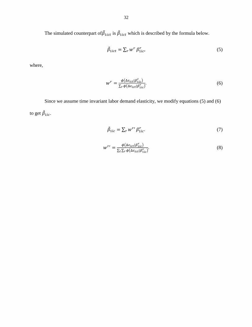
32
The simulated counterpart of�̅�1𝑖𝑐𝑡 is �̌�1𝑖𝑐𝑡 which is described by the formula below.
�̌�1𝑖𝑐𝑡 = ∑ 𝑤𝑟𝑟 𝛽1𝑖𝑐𝑟 , (5)
where,
𝑤𝑟 =𝜙(Δ 𝑖𝑐𝑡|𝛽1𝑖𝑐
𝑟 )
∑ 𝜙(Δ 𝑖𝑐𝑡|𝛽1𝑖𝑐𝑟 )𝑟. (6)
Since we assume time invariant labor demand elasticity, we modify equations (5) and (6)
to get �̌�1𝑖𝑐.
�̌�1𝑖𝑐 = ∑ 𝑤𝑟′𝑟 𝛽1𝑖𝑐𝑟 . (7)
𝑤𝑟′ =𝜙(Δ 𝑖𝑐𝑡|𝛽1𝑖𝑐
𝑟 )
∑ ∑ 𝜙(Δ 𝑖𝑐𝑡|𝛽1𝑖𝑐𝑟 )𝑟𝑡. (8)
33
(D) Some additional plots
Notes: Producer and Consumer price index data are from the Bureau of Labor Statistics. Military contracts data is from
U.S. Census Bureau. Natural amenity scale data is from United States Department of Agriculture.
34
Notes: Employment data is from County Business Patterns.
8. Figures and Tables
Figure 1: Total national industry employment
35
Figure 2: National industry total real output
Notes: Industry real output is calculated by deflating nominal output using the Producer Price Index. Nominal
output data is from the Bureau of Economic Analysis (BEA). Producer Price Index data is from the Bureau of
Labor Statistics.
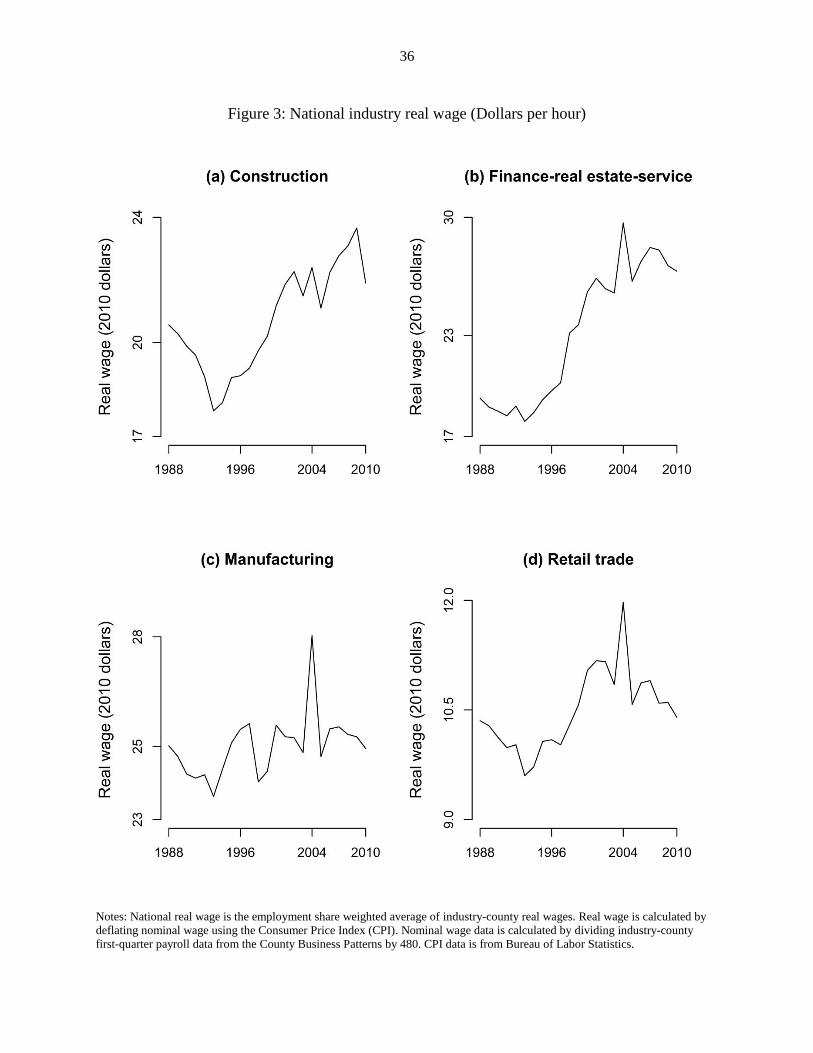
36
Notes: National real wage is the employment share weighted average of industry-county real wages. Real wage is calculated by
deflating nominal wage using the Consumer Price Index (CPI). Nominal wage data is calculated by dividing industry-county
first-quarter payroll data from the County Business Patterns by 480. CPI data is from Bureau of Labor Statistics.
Figure 3: National industry real wage (Dollars per hour)
37
Notes: The above graph shows the weighted average industry-county own wage labor demand
elasticity for counties in the conterminous U.S. The industries included in the average are:
construction, finance/insurance/real-estate/service, manufacturing, and retail trade. The weights
are constructed using the average industry-county employments in the period 1988-2010.
Figure 4: Regional variations in labor demand elasticity
38
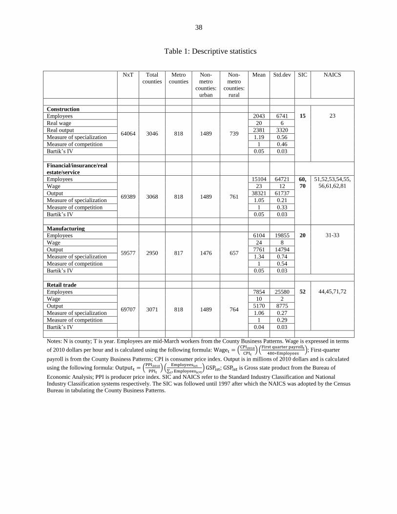
Table 1: Descriptive statistics
NxT Total
counties
Metro
counties
Non-
metro
counties:
urban
Non-
metro
counties:
rural
Mean Std.dev SIC NAICS
Construction
15
23 Employees
64064 3046 818 1489 739
2043 6741
Real wage 20 6
Real output 2381 3320
Measure of specialization 1.19 0.56
Measure of competition 1 0.46
Bartik’s IV 0.05 0.03
Financial/insurance/real
estate/service
Employees
69389 3068 818 1489 761
15104 64721 60,
70
51,52,53,54,55,
56,61,62,81 Wage 23 12
Output 38321 61737
Measure of specialization 1.05 0.21
Measure of competition 1 0.33
Bartik’s IV 0.05 0.03
Manufacturing
20
31-33 Employees
59577 2950 817 1476 657
6104 19855
Wage 24 8
Output 7761 14794
Measure of specialization 1.34 0.74
Measure of competition 1 0.54
Bartik’s IV 0.05 0.03
Retail trade
52
44,45,71,72 Employees
69707 3071 818 1489 764
7854 25580
Wage 10 2
Output 5170 8775
Measure of specialization 1.06 0.27
Measure of competition 1 0.29
Bartik’s IV 0.04 0.03
Notes: N is county; T is year. Employees are mid-March workers from the County Business Patterns. Wage is expressed in terms
of 2010 dollars per hour and is calculated using the following formula: Waget = (CPI2010
CPIt) (
First quarter payrollt
480∗Employees); First-quarter
payroll is from the County Business Patterns; CPI is consumer price index. Output is in millions of 2010 dollars and is calculated
using the following formula: Outputt = (PPI2010
PPIt) (
Employeesict
∑ Employeesic′tc′)GSPist; GSPist is Gross state product from the Bureau of
Economic Analysis; PPI is producer price index. SIC and NAICS refer to the Standard Industry Classification and National
Industry Classification systems respectively. The SIC was followed until 1997 after which the NAICS was adopted by the Census
Bureau in tabulating the County Business Patterns.
39
Table 2: States with right to work laws
State Year of Statue Enactment Year of Constitutional Amendment
ALABAMA 1953
ARIZONA 1947 1946
ARKANSAS 1947 1944
FLORIDA 1943 1968
GEORGIA 1947
IDAHO 1985
INDIANA 2012
IOWA 1947
KANSAS 1958
LOUISIANA 1976
MICHIGAN 2012
MISSISSIPPI 1954 1960
NEBRASKA 1947 1946
NEVADA 1951 1952
NORTH CAROLINA 1947
NORTH DAKOTA 1947 1948
OKLAHOMA 2001 2001
SOUTH CAROLINA 1954
SOUTH DAKOTA 1947 1946
TENNESSEE 1947
TEXAS 1993
UTAH 1955
VIRGINIA 1947
WYOMING 1963
Notes: Data is from the National Conference of State Legislatures.
40
Table 3: Estimates of wage elasticity of labor demand
Industry NxT Model Estimation 𝛽1
Δlog(wage)
𝛽1𝑖 𝛾𝑖 𝛽2
Δlog(output)
𝑅2 log
likelihood √𝜎 𝑖2
Construction 61018
(1)
Constant
parameter
OLS -0.01***
(0.004)
--- --- 0.92***
(0.004)
0.90
--- 0.07
(2) OLS+CF
-0.14***
(0.01)
--- --- 0.48***
(0.01)
0.71
--- 0.12
(3) Random
parameter
MSL 0.02
[0.07]
-4.75***
(0.15)
0.39***
(0.04)
0.84***
(0.002)
--- 46717 0.05
(4) MSL+CF
0.15
[0.13]
-2.17***
(0.04)
-0.51***
(0.03)
0.48***
(0.01)
--- 76668 0.06
Finance/insurance/
real-estate/service 66321
(1)
Constant
parameter
OLS -0.03***
(0.005)
--- --- 0.93***
(0.006)
0.92
--- 0.06
(2) OLS+CF -0.02
(0.03)
--- --- 0.18***
(0.02)
0.33
--- 0.20
(3)
Random
parameter
MSL 0.10
[1.35]
-4.76***
(0.14)
0.81***
(0.02)
0.90***
(0.001)
--- 65100 0.04
(4) MSL+CF 0.005
[0.05]
-7.4***
(0.02)
1.49***
(0.002)
0.20***
(0.007)
--- 98217 0.04
Manufacturing 56627
(1)
Constant
parameter
OLS -0.07***
(0.01)
--- --- 0.78***
(0.01)
0.74
--- 0.10
(2) OLS+CF -0.24***
(0.03)
--- --- 0.05
(0.04)
0.12
--- 0.19
(3)
Random
parameter
MSL 0.11
[1.85]
-4.90***
(0.10)
0.85***
(0.01)
0.69***
(0.002)
--- 29840 0.07
(4) MSL+CF 0.21
[0.38]
-2.28***
(0.05)
0.37***
(0.01)
-0.02 --- 49887 0.09
Retail trade 66636
(1)
Constant
parameter
OLS -0.05***
(0.01)
--- --- 0.80***
(0.01)
0.78
--- 0.07
(2) OLS+CF -0.17***
(0.04)
--- --- 0.12***
(0.01)
0.22
--- 0.14
(3)
Random
parameter
MSL 0.08
[0.38]
-3.95***
(0.12)
0.55***
(0.02)
0.68***
(0.002)
--- 55136 0.05
(4) MSL+CF
0.09
[0.25]
-3.47***
(0.03)
0.77***
(0.005)
0.13***
(0.005)
--- 95876 0.05
Notes: N = Number of counties; T = Number of years. In constant parameter regression estimations dependent variable is ∆log(𝐿𝑖𝑐𝑡).Clustered
standard error in parenthesis; cluster ID is BEA economic zone. �̅�1 = 𝑒𝑥𝑝[𝛽1 + 0.5𝑒𝑥𝑝(𝛾)2] is mean of log normal distribution.√𝜎𝛽1
2 =
𝑒𝑥𝑝[𝑒𝑥𝑝(𝛾)2 − 1]𝑒𝑥𝑝[2𝛽1 + 𝑒𝑥𝑝(𝛾)2] is standard deviation of log normal distribution. Significance levels: * p<0.1, ** p<0.05, *** p<0.01.
CF stands for Control Function, MSL stands for Maximum Simulated Likelihood.
41
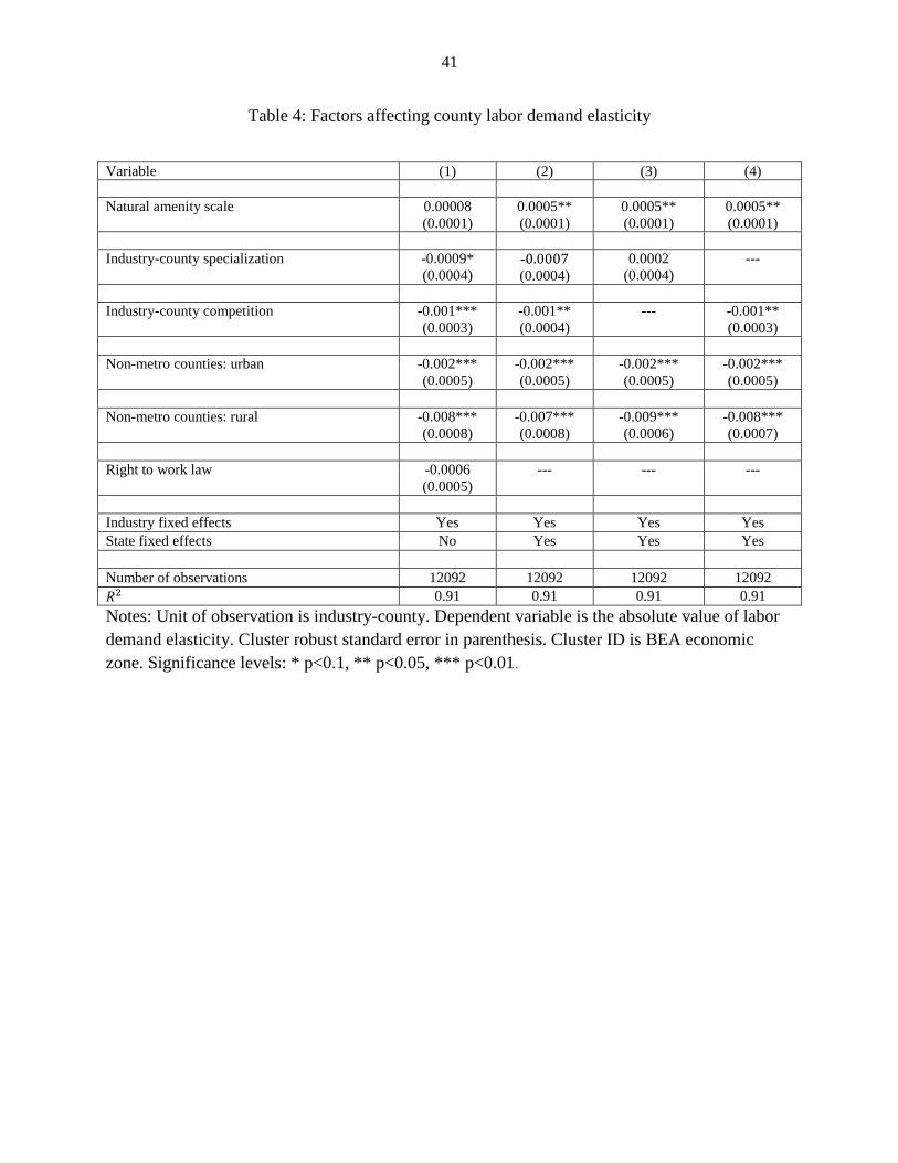
Table 4: Factors affecting county labor demand elasticity
Variable (1) (2) (3) (4)
Natural amenity scale 0.00008
(0.0001)
0.0005**
(0.0001)
0.0005**
(0.0001)
0.0005**
(0.0001)
Industry-county specialization -0.0009*
(0.0004) -0.0007
(0.0004)
0.0002
(0.0004)
---
Industry-county competition -0.001***
(0.0003)
-0.001**
(0.0004)
--- -0.001**
(0.0003)
Non-metro counties: urban -0.002***
(0.0005)
-0.002***
(0.0005)
-0.002***
(0.0005)
-0.002***
(0.0005)
Non-metro counties: rural -0.008***
(0.0008)
-0.007***
(0.0008)
-0.009***
(0.0006)
-0.008***
(0.0007)
Right to work law -0.0006
(0.0005)
--- --- ---
Industry fixed effects Yes Yes Yes Yes
State fixed effects No Yes Yes Yes
Number of observations 12092 12092 12092 12092
𝑅2 0.91 0.91 0.91 0.91
Notes: Unit of observation is industry-county. Dependent variable is the absolute value of labor
demand elasticity. Cluster robust standard error in parenthesis. Cluster ID is BEA economic
zone. Significance levels: * p<0.1, ** p<0.05, *** p<0.01.
42
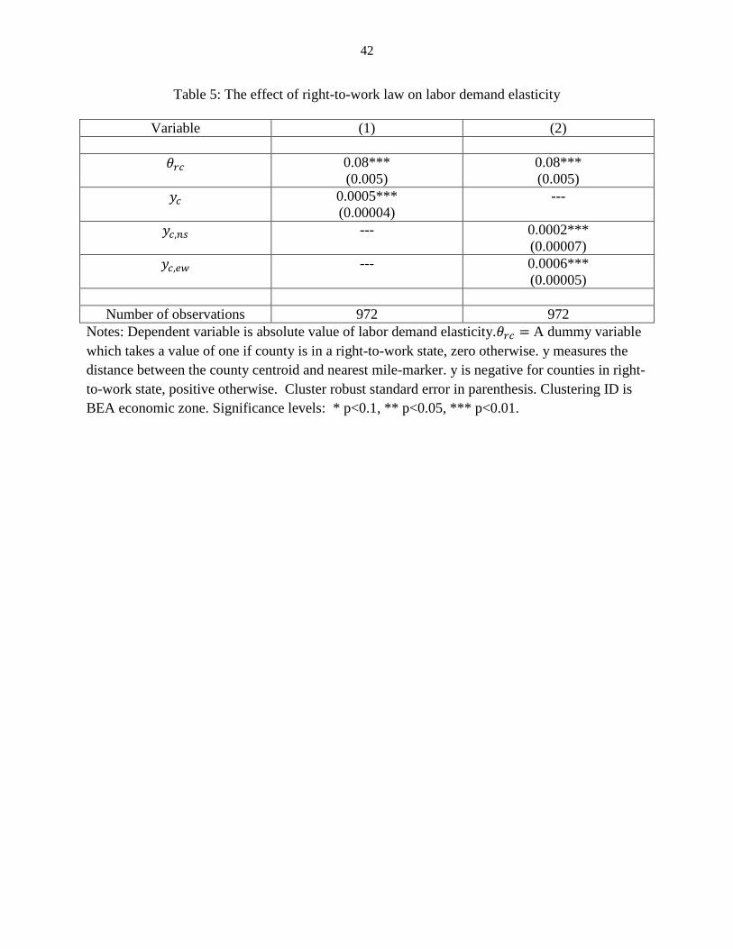
Table 5: The effect of right-to-work law on labor demand elasticity
Variable (1) (2)
𝜃𝑟𝑐 0.08***
(0.005)
0.08***
(0.005)
𝑦𝑐 0.0005***
(0.00004)
---
𝑦𝑐,𝑛𝑠 --- 0.0002***
(0.00007)
𝑦𝑐,𝑒𝑤 --- 0.0006***
(0.00005)
Number of observations 972 972
Notes: Dependent variable is absolute value of labor demand elasticity.𝜃𝑟𝑐 = A dummy variable
which takes a value of one if county is in a right-to-work state, zero otherwise. y measures the
distance between the county centroid and nearest mile-marker. y is negative for counties in right-
to-work state, positive otherwise. Cluster robust standard error in parenthesis. Clustering ID is
BEA economic zone. Significance levels: * p<0.1, ** p<0.05, *** p<0.01.