Embed Size (px)
Citation preview


Sebastian Hack
Register Allocation for Programs in SSA Form

Register Allocation forPrograms in SSA Form
by Sebastian Hack
Impressum
Universitätsverlag Karlsruhec/o UniversitätsbibliothekStraße am Forum 2D-76131 Karlsruhewww.uvka.de
Dieses Werk ist unter folgender Creative Commons-Lizenz lizenziert: http://creativecommons.org/licenses/by-nc-nd/2.0/de/
Universitätsverlag Karlsruhe 2007 Print on Demand
ISBN: 978-3-86644-180-4
Dissertation, Universität Karlsruhe (TH)Fakultät für Informatik, 2006


Register Allocation for Programs in SSA Form
zur Erlangung des akademischen Grades eines
Doktors der Naturwissenschaften
der Fakultat fur Informatikder Universitat Fridericiana zu Karlsruhe (TH)
genehmigte
Dissertation
von
Sebastian Hack
aus Heidelberg
Tag der mundlichen Prufung: 31.10.2006Erster Gutachter: Prof. em. Dr. Dr. h. c. Gerhard GoosZweiter Gutachter: Prof. Dr. Alan Mycroft

Acknowledgements
This thesis is the result of the research I did at the chair of Prof. Goos at theUniversitat Karlsruhe from May 2004 until October 2006. In these two and ahalf years I had the chance to meet, work and be with so many great people.I here want to take the opportunity to express my gratitude to them.
I am very obliged to Gerhard Goos. He supported my thesis from the verybeginning and was at any time open for discussions not only regarding thethesis. I definitely learned a lot from him. I thank him for granting me thenecessary freedom to pursue my ideas, for his faith in me and all the supportI received from him.
Alan Mycroft very unexpectedly invited my to Cambridge to give a talkabout my early results. I enjoyed many discussions with him and am verythankful for his advice and support through the years as well as being theexternal examiner for this thesis.
Both referees provided many excellent comments which improved this the-sis significantly.
I am very thankful to my colleagues Mamdouh Abu-Sakran, Michael Beck,Boris Boesler, Rubino Geiß, Dirk Heuzeroth, Florian Liekweg, Gotz Linden-maier, Markus Noga, Bernd Traub and Katja Weißhaupt for such a pleasanttime in Karlsruhe, their friendship and many interesting and fruitful discus-sions and conversations from which I had the chance to learn so much; notonly regarding computer science.
I had immense help from many master students in Karlsruhe to realisethis project. Their scientific vitality was essential for my work. I already misstheir extraordinary dedication and the high quality of their work. Thank youVeit Batz, Matthias Braun, Daniel Grund, Kimon Hoffmann, Enno Hofmann,Hannes Jakschitsch, Moritz Kroll, Christoph Mallon, Johannes Spallek, AdamM. Szalkowski and Christian Wurdig.
I would also like to thank many people outside Karlsruhe who helped toimprove my research with many insightful discussions. I would like to thank:
ix
x
Benoit Boissinot, Florent Bouchez, Philip Brisk, Alain Darte, Jens Palsberg,Fernando Pereira, Fabrice Rastello and Simon Peyton-Jones.
I thank Andre Rupp for the many opportunities he opened for me and hisfriendship over the last years.
Nothing would have been possible without my family. I thank my parentsand my brother for their support. My beloved wife Kerstin accompanied methrough all the ups and downs a PhD thesis implies and always supportedme. Thank you for being there.
Lyon, September 2007Sebastian Hack
Contents
List of Symbols xv
1 Introduction 1
1.1 Graph-Coloring Register Allocation . . . . . . . . . . . . . . . . 21.2 SSA-based Register Allocation . . . . . . . . . . . . . . . . . . 31.3 Overview of this Thesis . . . . . . . . . . . . . . . . . . . . . . 6
2 Foundations 7
2.1 Lists and Linearly Ordered Sets . . . . . . . . . . . . . . . . . . 72.2 Programs . . . . . . . . . . . . . . . . . . . . . . . . . . . . . . 82.3 Static Single Assignment (SSA) . . . . . . . . . . . . . . . . . . 11
2.3.1 Semantics of Φ-operations . . . . . . . . . . . . . . . . . 122.3.2 Non-Strict Programs and the Dominance Property . . . 132.3.3 SSA Destruction . . . . . . . . . . . . . . . . . . . . . . 15
2.4 Global Register Allocation . . . . . . . . . . . . . . . . . . . . . 162.4.1 Interference . . . . . . . . . . . . . . . . . . . . . . . . . 172.4.2 Coalescing and Live Range Splitting . . . . . . . . . . . 182.4.3 Spilling . . . . . . . . . . . . . . . . . . . . . . . . . . . 192.4.4 Register Targeting . . . . . . . . . . . . . . . . . . . . . 21
3 State of the Art 23
3.1 Graph-Coloring Register Allocation . . . . . . . . . . . . . . . . 243.1.1 Extensions to the Chaitin-Allocator . . . . . . . . . . . 263.1.2 Splitting-Based Approaches . . . . . . . . . . . . . . . . 283.1.3 Region-Based Approaches . . . . . . . . . . . . . . . . . 293.1.4 Other Graph-Coloring Approaches . . . . . . . . . . . . 303.1.5 Practical Considerations . . . . . . . . . . . . . . . . . . 31
xi
xii Contents
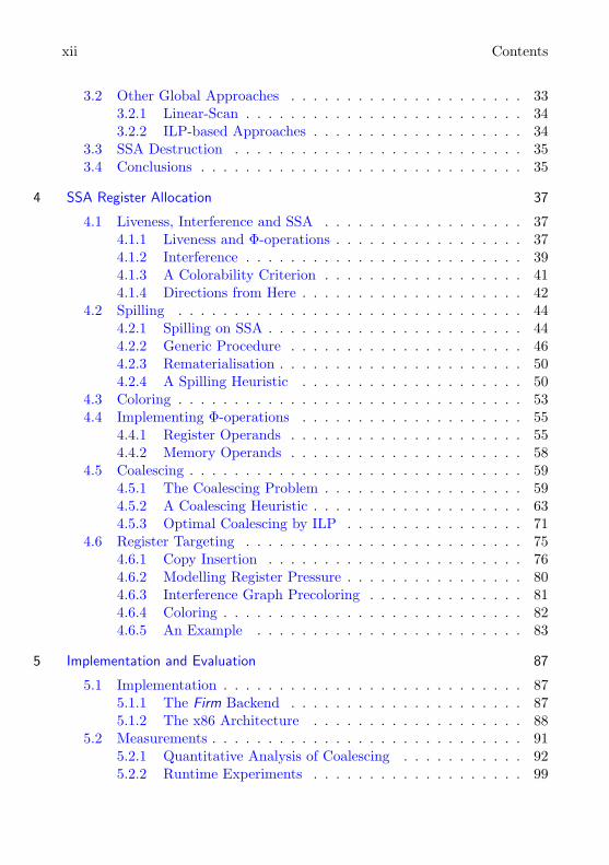
3.2 Other Global Approaches . . . . . . . . . . . . . . . . . . . . . 333.2.1 Linear-Scan . . . . . . . . . . . . . . . . . . . . . . . . . 343.2.2 ILP-based Approaches . . . . . . . . . . . . . . . . . . . 34
3.3 SSA Destruction . . . . . . . . . . . . . . . . . . . . . . . . . . 353.4 Conclusions . . . . . . . . . . . . . . . . . . . . . . . . . . . . . 35
4 SSA Register Allocation 37
4.1 Liveness, Interference and SSA . . . . . . . . . . . . . . . . . . 374.1.1 Liveness and Φ-operations . . . . . . . . . . . . . . . . . 374.1.2 Interference . . . . . . . . . . . . . . . . . . . . . . . . . 394.1.3 A Colorability Criterion . . . . . . . . . . . . . . . . . . 414.1.4 Directions from Here . . . . . . . . . . . . . . . . . . . . 42
4.2 Spilling . . . . . . . . . . . . . . . . . . . . . . . . . . . . . . . 444.2.1 Spilling on SSA . . . . . . . . . . . . . . . . . . . . . . . 444.2.2 Generic Procedure . . . . . . . . . . . . . . . . . . . . . 464.2.3 Rematerialisation . . . . . . . . . . . . . . . . . . . . . . 504.2.4 A Spilling Heuristic . . . . . . . . . . . . . . . . . . . . 50
4.3 Coloring . . . . . . . . . . . . . . . . . . . . . . . . . . . . . . . 534.4 Implementing Φ-operations . . . . . . . . . . . . . . . . . . . . 55
4.4.1 Register Operands . . . . . . . . . . . . . . . . . . . . . 554.4.2 Memory Operands . . . . . . . . . . . . . . . . . . . . . 58
4.5 Coalescing . . . . . . . . . . . . . . . . . . . . . . . . . . . . . . 594.5.1 The Coalescing Problem . . . . . . . . . . . . . . . . . . 594.5.2 A Coalescing Heuristic . . . . . . . . . . . . . . . . . . . 634.5.3 Optimal Coalescing by ILP . . . . . . . . . . . . . . . . 71
4.6 Register Targeting . . . . . . . . . . . . . . . . . . . . . . . . . 754.6.1 Copy Insertion . . . . . . . . . . . . . . . . . . . . . . . 764.6.2 Modelling Register Pressure . . . . . . . . . . . . . . . . 804.6.3 Interference Graph Precoloring . . . . . . . . . . . . . . 814.6.4 Coloring . . . . . . . . . . . . . . . . . . . . . . . . . . . 824.6.5 An Example . . . . . . . . . . . . . . . . . . . . . . . . 83
5 Implementation and Evaluation 87
5.1 Implementation . . . . . . . . . . . . . . . . . . . . . . . . . . . 875.1.1 The Firm Backend . . . . . . . . . . . . . . . . . . . . . 875.1.2 The x86 Architecture . . . . . . . . . . . . . . . . . . . 88
5.2 Measurements . . . . . . . . . . . . . . . . . . . . . . . . . . . . 915.2.1 Quantitative Analysis of Coalescing . . . . . . . . . . . 925.2.2 Runtime Experiments . . . . . . . . . . . . . . . . . . . 99
Contents xiii
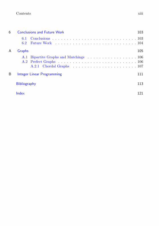
6 Conclusions and Future Work 103
6.1 Conclusions . . . . . . . . . . . . . . . . . . . . . . . . . . . . . 1036.2 Future Work . . . . . . . . . . . . . . . . . . . . . . . . . . . . 104
A Graphs 105
A.1 Bipartite Graphs and Matchings . . . . . . . . . . . . . . . . . 106A.2 Perfect Graphs . . . . . . . . . . . . . . . . . . . . . . . . . . . 106
A.2.1 Chordal Graphs . . . . . . . . . . . . . . . . . . . . . . 107
B Integer Linear Programming 111
Bibliography 113
Index 121

xiv Contents
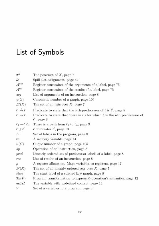
List of Symbols
2X The powerset of X, page 7
& Spill slot assignment, page 44
Aarg Register constraints of the arguments of a label, page 75
Ares Register constraints of the results of a label, page 75
arg List of arguments of an instruction, page 8
χ(G) Chromatic number of a graph, page 106
L (X) The set of all lists over X, page 7
`′i→ ` Predicate to state that the i-th predecessor of ` is `′, page 8
`′ → ` Predicate to state that there is a i for which ` is the i-th predecessor of`′, page 8
`1 →∗ `n There is a path from `1 to `n, page 9
` � `′ ` dominates `′, page 10
L Set of labels in the program, page 8
m A memory variable, page 44
ω(G) Clique number of a graph, page 105
op Operation of an instruction, page 8
pred Linearly ordered set of predecessor labels of a label, page 8
res List of results of an instruction, page 8
ρ A register allocation. Maps variables to registers, page 17
S (X) The set of all linearly ordered sets over X, page 7
start The start label of a control flow graph, page 8
TΦ(P ) Program transformation to express Φ-operation’s semantics, page 12
undef The variable with undefined content, page 14
V Set of a variables in a program, page 8
xv

xvi Contents
1 Introduction
One major benefit of higher-level programming languages over machine codeis, that the programmer is relieved of assigning storage locations to the val-ues the program is processing. To store the results of computations, almostevery processor provides a set of registers with very fast access. However, thenumber of registers is often very small, usually from 8 to 32. So, for complexcomputations there might not be enough registers available. Then, some ofthe computed values have to be put into memory which is, in comparisonto the register bank, huge but much slower to access. Generally, one talksabout a memory hierarchy where the larger a memory is, the slower it is toaccess. The processor’s registers represent the smallest and fastest end of thishierarchy.
Common programming languages do not pay attention to the memory hi-erarchy for several reasons. First of all, the number, size and speed of thedifferent kinds of memory differ from one machine to another. Secondly, theprogrammer should be relieved of considering all the details concerning theunderlying hardware architecture since the program should efficiently run onas many architectures as possible. These details are covered by the compiler,which translates the program as it is written by the programmer into ma-chine code. Since the compiler targets a single processor architecture in sucha translation process, it takes care of these details in order to produce effi-cient code for the processor. Thus, the compiler should be concerned aboutassigning as many variables as possible to processor registers. In the case thatthe number of registers available does not suffice the compiler has to carefullydecide which variables will reside in main memory. This whole task is calledregister allocation.
The principle of register allocation is simple: the compiler has to determinefor each point in the program which variables are live, i.e. will be needed insome computation later on. If two variables being live at the same point in theprogram, i.e. they are still needed in some future computation, they must not
1
2 Introduction
occupy the same storage location, especially not the same register. We thensay the variables interfere. The register allocator then has to assign a registerto each variable while ensuring that all interfering variables have differentregisters. However, if the register allocator determines that the number ofregisters does not suffice to meet the demand of the program, it has to modifythe program by inserting explicit memory accesses for variables that could notbe assigned a register. This part, called spilling , is crucial since memory accessis comparatively slow. To quote [Hennessy and Patterson, 1997, page 92]:
Because of the central role that register allocation plays, bothin speeding up the code and in making other optimizations use-ful, it is one of the most important—if not the most important—optimizations.
1.1 Graph-Coloring Register Allocation
The most prominent approach to register allocation probably is graph col-oring . Thereby, interference is represented as a graph: each variable in theprogram corresponds to a node in the graph. Whenever two variables in-terfere, the respective nodes are connected by an edge. As we want to mapthe variables to registers, we assign registers to the nodes in the interferencegraph so that two adjacent nodes are assigned different registers.
In graph theory, such a mapping is called a coloring.1 The major problemis that an optimal coloring, i.e. one using as few colors as possible, is generallyhard to compute; it is NP-complete. Furthermore, the problems of checking agraph for its k-colorability and the problem of finding its chromatic number,i.e. the smallest number of colors needed to achieve a valid coloring of thegraph, are also NP-complete. In his seminal work, Chaitin et al. [1981] showedthat each graph is the interference graph of some program. Thus, registerallocation is NP-complete, also.
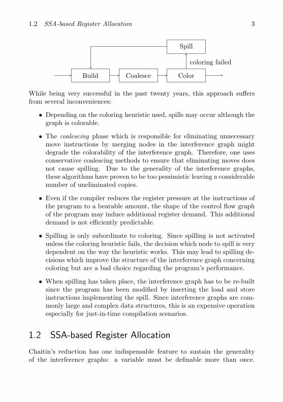
To color the interference graph, usually a heuristic is applied. The vari-ables which have to be spilled are determined during coloring when a nodecannot be assigned a color by the heuristic. This leads to an iterative approachas shown below:
1The term coloring originates from the famous four color problem: Given a map, arefour colors sufficient to color the countries on the map in a way that two adjacent countrieshave different colors? This question was positively answered in 1974 after being an openquestion for more than 100 years.
1.2 SSA-based Register Allocation 3
Build Coalesce Color
Spill
coloring failed
While being very successful in the past twenty years, this approach suffersfrom several inconveniences:
• Depending on the coloring heuristic used, spills may occur although thegraph is colorable.
• The coalescing phase which is responsible for eliminating unnecessarymove instructions by merging nodes in the interference graph mightdegrade the colorability of the interference graph. Therefore, one usesconservative coalescing methods to ensure that eliminating moves doesnot cause spilling. Due to the generality of the interference graphs,these algorithms have proven to be too pessimistic leaving a considerablenumber of uneliminated copies.
• Even if the compiler reduces the register pressure at the instructions ofthe program to a bearable amount, the shape of the control flow graphof the program may induce additional register demand. This additionaldemand is not efficiently predictable.
• Spilling is only subordinate to coloring. Since spilling is not activatedunless the coloring heuristic fails, the decision which node to spill is verydependent on the way the heuristic works. This may lead to spilling de-cisions which improve the structure of the interference graph concerningcoloring but are a bad choice regarding the program’s performance.
• When spilling has taken place, the interference graph has to be re-builtsince the program has been modified by inserting the load and storeinstructions implementing the spill. Since interference graphs are com-monly large and complex data structures, this is an expensive operationespecially for just-in-time compilation scenarios.
1.2 SSA-based Register Allocation
Chaitin’s reduction has one indispensable feature to sustain the generalityof the interference graphs: a variable must be definable more than once.
4 Introduction
This especially means that if a variable is defined multiple times, all valuescomputed at these definitions must be written to the same register. Whilethis seems to be an obvious presumption, it allows for generating arbitraryinterferences and thus arbitrary interference graphs.
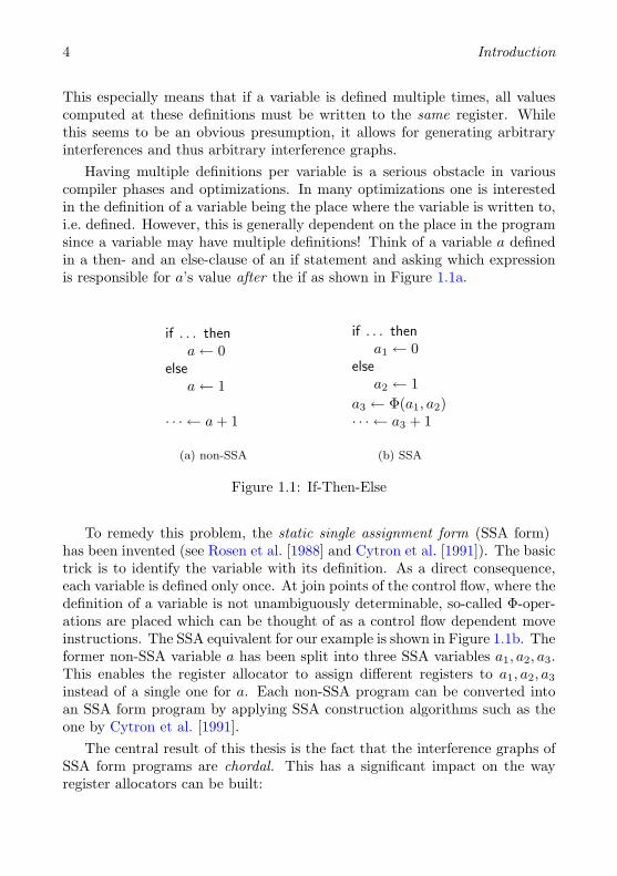
Having multiple definitions per variable is a serious obstacle in variouscompiler phases and optimizations. In many optimizations one is interestedin the definition of a variable being the place where the variable is written to,i.e. defined. However, this is generally dependent on the place in the programsince a variable may have multiple definitions! Think of a variable a definedin a then- and an else-clause of an if statement and asking which expressionis responsible for a’s value after the if as shown in Figure 1.1a.
if . . . thena← 0
elsea← 1
· · · ← a + 1
(a) non-SSA
if . . . thena1 ← 0
elsea2 ← 1
a3 ← Φ(a1, a2)· · · ← a3 + 1
(b) SSA
Figure 1.1: If-Then-Else
To remedy this problem, the static single assignment form (SSA form)has been invented (see Rosen et al. [1988] and Cytron et al. [1991]). The basictrick is to identify the variable with its definition. As a direct consequence,each variable is defined only once. At join points of the control flow, where thedefinition of a variable is not unambiguously determinable, so-called Φ-oper-ations are placed which can be thought of as a control flow dependent moveinstructions. The SSA equivalent for our example is shown in Figure 1.1b. Theformer non-SSA variable a has been split into three SSA variables a1, a2, a3.This enables the register allocator to assign different registers to a1, a2, a3
instead of a single one for a. Each non-SSA program can be converted intoan SSA form program by applying SSA construction algorithms such as theone by Cytron et al. [1991].
The central result of this thesis is the fact that the interference graphs ofSSA form programs are chordal. This has a significant impact on the wayregister allocators can be built:
1.2 SSA-based Register Allocation 5
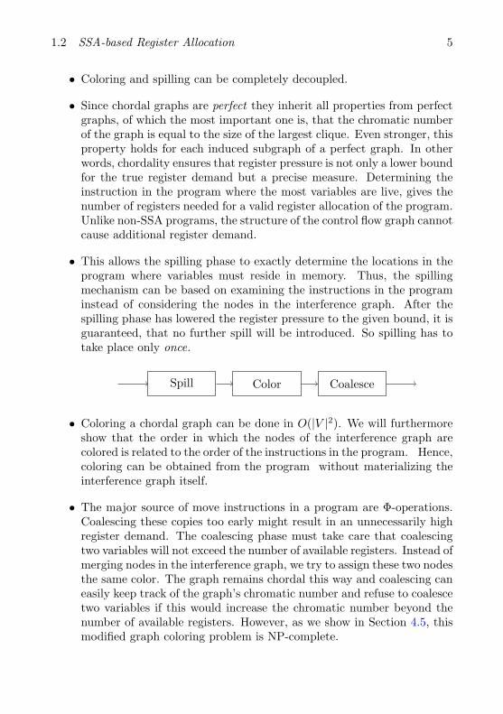
• Coloring and spilling can be completely decoupled.
• Since chordal graphs are perfect they inherit all properties from perfectgraphs, of which the most important one is, that the chromatic numberof the graph is equal to the size of the largest clique. Even stronger, thisproperty holds for each induced subgraph of a perfect graph. In otherwords, chordality ensures that register pressure is not only a lower boundfor the true register demand but a precise measure. Determining theinstruction in the program where the most variables are live, gives thenumber of registers needed for a valid register allocation of the program.Unlike non-SSA programs, the structure of the control flow graph cannotcause additional register demand.
• This allows the spilling phase to exactly determine the locations in theprogram where variables must reside in memory. Thus, the spillingmechanism can be based on examining the instructions in the programinstead of considering the nodes in the interference graph. After thespilling phase has lowered the register pressure to the given bound, it isguaranteed, that no further spill will be introduced. So spilling has totake place only once.
Spill Color Coalesce
• Coloring a chordal graph can be done in O(|V |2). We will furthermoreshow that the order in which the nodes of the interference graph arecolored is related to the order of the instructions in the program. Hence,coloring can be obtained from the program without materializing theinterference graph itself.
• The major source of move instructions in a program are Φ-operations.Coalescing these copies too early might result in an unnecessarily highregister demand. The coalescing phase must take care that coalescingtwo variables will not exceed the number of available registers. Instead ofmerging nodes in the interference graph, we try to assign these two nodesthe same color. The graph remains chordal this way and coalescing caneasily keep track of the graph’s chromatic number and refuse to coalescetwo variables if this would increase the chromatic number beyond thenumber of available registers. However, as we show in Section 4.5, thismodified graph coloring problem is NP-complete.
6 Introduction
1.3 Overview of this Thesis
Chapter 2 provides notational foundations and a more precise introductionto the register allocation problem and its components. Chapter 3 gives anoverview over the state of register allocation research that is relevant andrelated to this thesis. Chapter 4 establishes the chordal property of the in-terference graphs of SSA form programs. Based on this theoretic foundation,methods and algorithms for spilling, coalescing and the treatment of registerconstraints are developed to exploit the benefits of SSA-based register allo-cation. Please note that this chapter makes intensive use of terminologyof the theory of perfect graphs. (Readers not familiar with this should readAppendix A beforehand). Afterwards, an experimental evaluation of the newregister allocator proposed is presented in Chapter 5. The thesis ends withfinal conclusions and an outlook to further research. Finally, Appendices Aand B provide the terms and definitions of graph theory and integer linearprogramming which are needed in this thesis.
2 Foundations
In this chapter we present the formal foundations needed throughout thisthesis.
2.1 Lists and Linearly Ordered Sets
In the following we often deal with lists and sets where the order of theelements matter. A list of length n over a carrier set X is defined as a totalmap s : {1, . . . , n} → X. The set of all lists of length n over X is denoted byL n(X). Furthermore
L (X) =⋃i∈N
L i(X)
represents the set of all lists over X. For a list s ∈ L (X) with s(1) =x1, . . . , s(n) = xn we shortly write (x1, . . . , xn). The i-th element of a list sis denoted by s(i). If there is some i for which s(i) = x we also write x ∈ s.
A linearly ordered set is a list in which no element occurs twice, i.e. themap s is injective. The set S (X) of linearly ordered sets over X is thusdefined as
S (X) = {s | s ∈ L (X) and s injective}
If a list (x1, . . . , xn) is also a linearly ordered set, we sometimes emphasizethis property by writing 〈x1, . . . , xn〉.
In the following, we often will deal with maps returning a list or a linearlyordered set. For example, let X and Y be two sets and a : X → L (Y ) besuch a map. Instead of writing a(x)(i) for accessing the i-th element of thereturned list, we will write a(x, i) according to the isomorphy of A→ (B → C)and (A×B)→ C.
7
8 Foundations
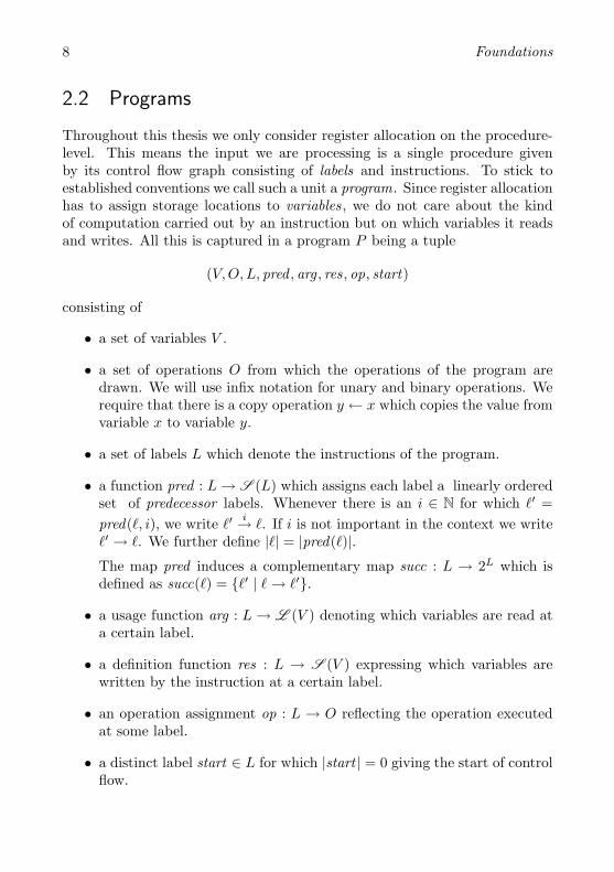
2.2 Programs
Throughout this thesis we only consider register allocation on the procedure-level. This means the input we are processing is a single procedure givenby its control flow graph consisting of labels and instructions. To stick toestablished conventions we call such a unit a program. Since register allocationhas to assign storage locations to variables, we do not care about the kindof computation carried out by an instruction but on which variables it readsand writes. All this is captured in a program P being a tuple
(V,O,L, pred , arg , res, op, start)
consisting of
• a set of variables V .
• a set of operations O from which the operations of the program aredrawn. We will use infix notation for unary and binary operations. Werequire that there is a copy operation y ← x which copies the value fromvariable x to variable y.
• a set of labels L which denote the instructions of the program.
• a function pred : L→ S (L) which assigns each label a linearly orderedset of predecessor labels. Whenever there is an i ∈ N for which `′ =pred(`, i), we write `′
i→ `. If i is not important in the context we write`′ → `. We further define |`| = |pred(`)|.The map pred induces a complementary map succ : L → 2L which isdefined as succ(`) = {`′ | `→ `′}.
• a usage function arg : L→ L (V ) denoting which variables are read ata certain label.
• a definition function res : L → S (V ) expressing which variables arewritten by the instruction at a certain label.
• an operation assignment op : L → O reflecting the operation executedat some label.
• a distinct label start ∈ L for which |start | = 0 giving the start of controlflow.
2.2 Programs 9
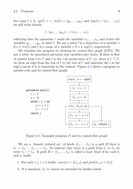
For some ` ∈ L, op(`) = τ , res(`) = (y1, . . . , ym) and arg(`) = (x1, . . . , xn)we will write shortly
` : (y1, . . . , ym)← τ (x1, . . . , xn)
reflecting that the operation τ reads the variables x1, . . . , xn and writes thevariables y1, . . . , ym at label `. We say a label ` is a definition of a variable xif x ∈ res(`) and ` is a usage of a variable x if x ∈ arg(`), respectively.
We visualize the program by drawing its control flow graph (CFG). Weput a label, its associated operation and variables into boxes. If there is flowof control from ` to `′ and ` is the i-th predecessor of `′, i.e. there is `
i→ `′,we draw an edge from the box of ` to the box of `′ and annotate the i at theedge’s arrow if it is important in the context. Figure 2.1 shows a program inpseudo-code and its control flow graph.
procedure sum(n)i← 1j ← 0while i ≤ n do
j ← j + ii← i + 1
return j
start : n← start
`1 : i← 1
`2 : j ← 0
`3 : if≤(i, n)
`4 : j ← j + i
`5 : i← i + 1 `6 : return j
Figure 2.1: Example program P and its control flow graph
We say a linearly ordered set of labels 〈`1, . . . , `n〉 is a path iff there is`1 → `2, . . . , `n−1 → `n. To indicate that there is a path from `1 to `n wewrite `1 →∗ `n. A path B = 〈`1, . . . , `n〉 is called a basic block if for each `i
and `j holds:
1. For each 1 ≤ i < n holds: succ(`i) = {`i+1} and pred(`i+1) = {`i}
2. B is maximal, i.e. it cannot be extended by further labels.
10 Foundations
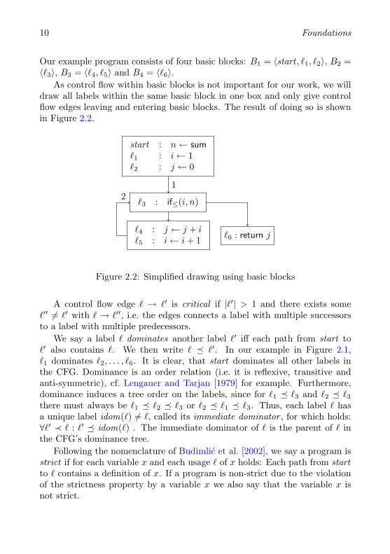
Our example program consists of four basic blocks: B1 = 〈start , `1, `2〉, B2 =〈`3〉, B3 = 〈`4, `5〉 and B4 = 〈`6〉.
As control flow within basic blocks is not important for our work, we willdraw all labels within the same basic block in one box and only give controlflow edges leaving and entering basic blocks. The result of doing so is shownin Figure 2.2.
start : n← sum`1 : i← 1`2 : j ← 0
`3 : if≤(i, n)
`4 : j ← j + i`5 : i← i + 1 `6 : return j
12
Figure 2.2: Simplified drawing using basic blocks
A control flow edge ` → `′ is critical if |`′| > 1 and there exists some`′′ 6= `′ with ` → `′′, i.e. the edges connects a label with multiple successorsto a label with multiple predecessors.
We say a label ` dominates another label `′ iff each path from start to`′ also contains `. We then write ` � `′. In our example in Figure 2.1,`1 dominates `2, . . . , `6. It is clear, that start dominates all other labels inthe CFG. Dominance is an order relation (i.e. it is reflexive, transitive andanti-symmetric), cf. Lengauer and Tarjan [1979] for example. Furthermore,dominance induces a tree order on the labels, since for `1 � `3 and `2 � `3there must always be `1 � `2 � `3 or `2 � `1 � `3. Thus, each label ` hasa unique label idom(`) 6= `, called its immediate dominator , for which holds:∀`′ ≺ ` : `′ � idom(`) . The immediate dominator of ` is the parent of ` inthe CFG’s dominance tree.
Following the nomenclature of Budimlic et al. [2002], we say a program isstrict if for each variable x and each usage ` of x holds: Each path from startto ` contains a definition of x. If a program is non-strict due to the violationof the strictness property by a variable x we also say that the variable x isnot strict.
2.3 Static Single Assignment (SSA) 11
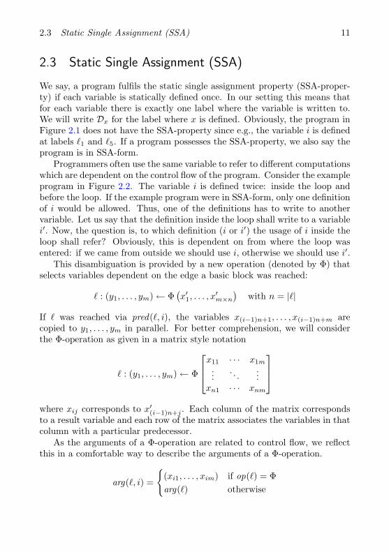
2.3 Static Single Assignment (SSA)
We say, a program fulfils the static single assignment property (SSA-proper-ty) if each variable is statically defined once. In our setting this means thatfor each variable there is exactly one label where the variable is written to.We will write Dx for the label where x is defined. Obviously, the program inFigure 2.1 does not have the SSA-property since e.g., the variable i is definedat labels `1 and `5. If a program possesses the SSA-property, we also say theprogram is in SSA-form.
Programmers often use the same variable to refer to different computationswhich are dependent on the control flow of the program. Consider the exampleprogram in Figure 2.2. The variable i is defined twice: inside the loop andbefore the loop. If the example program were in SSA-form, only one definitionof i would be allowed. Thus, one of the definitions has to write to anothervariable. Let us say that the definition inside the loop shall write to a variablei′. Now, the question is, to which definition (i or i′) the usage of i inside theloop shall refer? Obviously, this is dependent on from where the loop wasentered: if we came from outside we should use i, otherwise we should use i′.
This disambiguation is provided by a new operation (denoted by Φ) thatselects variables dependent on the edge a basic block was reached:
` : (y1, . . . , ym)← Φ(x′1, . . . , x
′m×n
)with n = |`|
If ` was reached via pred(`, i), the variables x(i−1)n+1, . . . , x(i−1)n+m arecopied to y1, . . . , ym in parallel. For better comprehension, we will considerthe Φ-operation as given in a matrix style notation
` : (y1, . . . , ym)← Φ
x11 · · · x1m
.... . .
...xn1 · · · xnm
where xij corresponds to x′(i−1)n+j . Each column of the matrix correspondsto a result variable and each row of the matrix associates the variables in thatcolumn with a particular predecessor.
As the arguments of a Φ-operation are related to control flow, we reflectthis in a comfortable way to describe the arguments of a Φ-operation.
arg(`, i) =
{(xi1, . . . , xim) if op(`) = Φarg(`) otherwise
12 Foundations
2.3.1 Semantics of Φ-operations
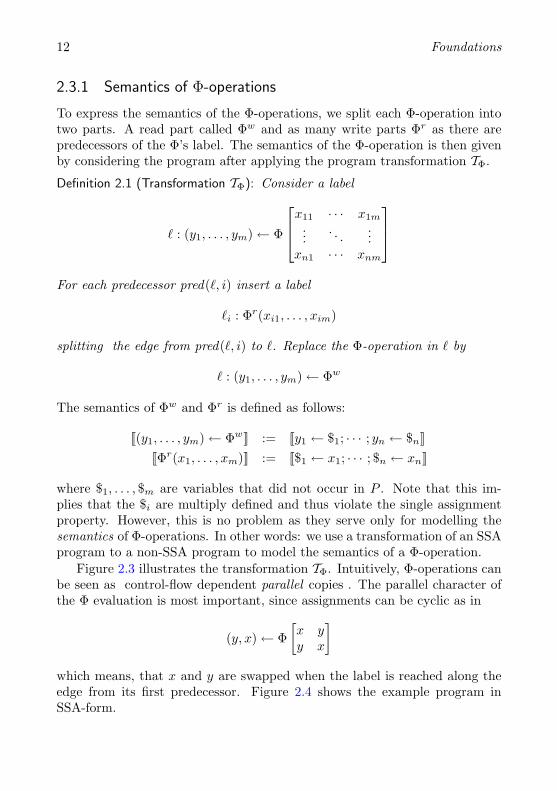
To express the semantics of the Φ-operations, we split each Φ-operation intotwo parts. A read part called Φw and as many write parts Φr as there arepredecessors of the Φ’s label. The semantics of the Φ-operation is then givenby considering the program after applying the program transformation TΦ.
Definition 2.1 (Transformation TΦ): Consider a label
` : (y1, . . . , ym)← Φ
x11 · · · x1m
.... . .
...xn1 · · · xnm
For each predecessor pred(`, i) insert a label
`i : Φr(xi1, . . . , xim)
splitting the edge from pred(`, i) to `. Replace the Φ-operation in ` by
` : (y1, . . . , ym)← Φw
The semantics of Φw and Φr is defined as follows:
J(y1, . . . , ym)← ΦwK := Jy1 ← $1; · · · ; yn ← $nKJΦr(x1, . . . , xm)K := J$1 ← x1; · · · ; $n ← xnK
where $1, . . . , $m are variables that did not occur in P . Note that this im-plies that the $i are multiply defined and thus violate the single assignmentproperty. However, this is no problem as they serve only for modelling thesemantics of Φ-operations. In other words: we use a transformation of an SSAprogram to a non-SSA program to model the semantics of a Φ-operation.
Figure 2.3 illustrates the transformation TΦ. Intuitively, Φ-operations canbe seen as control-flow dependent parallel copies . The parallel character ofthe Φ evaluation is most important, since assignments can be cyclic as in
(y, x)← Φ[x yy x
]which means, that x and y are swapped when the label is reached along theedge from its first predecessor. Figure 2.4 shows the example program inSSA-form.
2.3 Static Single Assignment (SSA) 13
(y1, y2)← Φ[x11 x12
x21 x22
]
A B
(a) A Φ-operation in some program P
(y1, y2)← Φw
Φr(x11, x12) Φr(x21, x22)
A B
(b) TΦ(P )
Figure 2.3: The program transformation TΦ
Remark 2.1: The matrix-style notation of Φ-instructions used in this thesisis not common in literature. Instead of a single Φ with a vector result anda matrix of operands one finds a φ for each column of the matrix with thearguments separated by commas. We find this misleading for two reasons:
1. it suggests that these φ-instructions are executed serially which is notthe case.
2. The commas make φ-instructions seem like each operand is needed to“compute” the results of the φ-instruction. This is also not the casesince only the i-th operand is needed when the φ’s label ` is reachedalong pred(`, i)
Figure 2.5 juxtaposes the style used in this thesis and the classical notation.
2.3.2 Non-Strict Programs and the Dominance Property
In principle, SSA-form programs can be non-strict (contain variables whichare not properly initialised). That is, there is a usage ` of some variable x forwhich there is a path from start to ` which does not contain Dx. However,almost every SSA-based algorithm only considers strict programs by relyingon the dominance property:
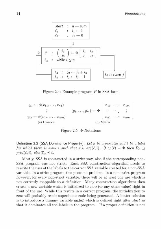
14 Foundations
start : n← sum`1 : i1 ← 1`2 : j1 ← 0
`′ :(
i3j3
)← Φ
[i1 i2j1 j2
]`3 : while i ≤ n
`4 : j2 ← j3 + i3`5 : i2 ← i3 + 1 `6 : return j
1
2
Figure 2.4: Example program P in SSA-form
y1 ← φ(x11, . . . , xn1)...
ym ← φ(x1m, . . . , xnm)(a) Classical
(y1, . . . , ym)← Φ
x11 · · · x1m
.... . .
...xn1 · · · xnm
(b) Matrix
Figure 2.5: Φ-Notations
Definition 2.2 (SSA Dominance Property): Let x be a variable and ` be a labelfor which there is some i such that x ∈ arg(`, i). If op(`) = Φ then Dx �pred(`, i), else Dx � `.
Mostly, SSA is constructed in a strict way, also if the corresponding non-SSA program was not strict. Each SSA construction algorithm needs torewrite the uses of the labels to the correct SSA variable created for a non-SSAvariable. In a strict program this poses no problem. In a non-strict programhowever, for every non-strict variable, there will be at least one use which isnot correctly mappable to a definition. Many construction algorithms thencreate a new variable which is initialized to zero (or any other value) right infront of the use. While this results in a correct program, the initialization tozero will probably result superfluous code being generated. A better solutionis to introduce a dummy variable undef which is defined right after start sothat it dominates all the labels in the program. If a proper definition is not
2.3 Static Single Assignment (SSA) 15
(y1, . . . , y3)← Φ[
x11 x12 x13
x21 x22 x23
](a) Program fragment
y1 ← x11
y2 ← x12
y3 ← x13
y1 ← x21
y2 ← x22
y3 ← x23
(b) Program fragment with copiesimplementing a Φ
Figure 2.6: SSA Destruction
(a3, b3)← Φ[
a1 b1
a2 b2
](a) SSA
a3 ← a1
b3 ← b1
(b) Post-SSA
Figure 2.7: Lost Copy Problem
found for some (non-strict) use, the use is rewritten to undef. Of course, nocode will ever be generated for the initialization of undef.
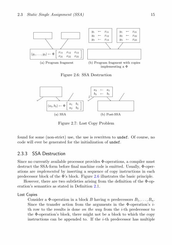
2.3.3 SSA Destruction
Since no currently available processor provides Φ-operations, a compiler mustdestruct the SSA-form before final machine code is emitted. Usually, Φ-oper-ations are implemented by inserting a sequence of copy instructions in eachpredecessor block of the Φ’s block. Figure 2.6 illustrates the basic principle.
However, there are two subtleties arising from the definition of the Φ-op-eration’s semantics as stated in Definition 2.1.
Lost CopiesConsider a Φ-operation in a block B having n predecessors B1, . . . , Bn.Since the transfer action from the arguments in the Φ-operation’s i-th row to the results is done on the way from the i-th predecessor tothe Φ-operation’s block, there might not be a block to which the copyinstructions can be appended to. If the i-th predecessor has multiple
16 Foundations
(a2, b2)← Φ[
b2 a2
· · · · · ·
](a) SSA
a2 ← b2
b2 ← a2
(b) Post-SSA
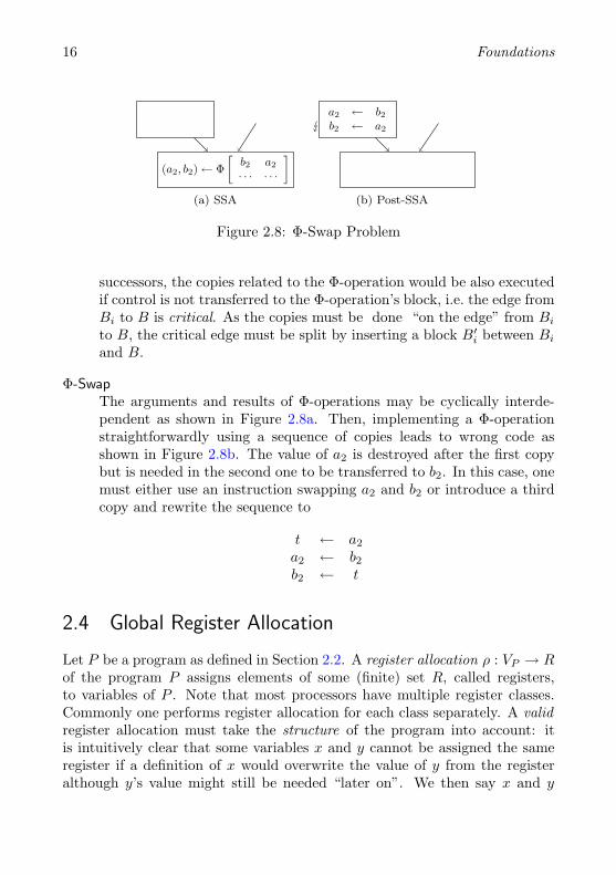
Figure 2.8: Φ-Swap Problem
successors, the copies related to the Φ-operation would be also executedif control is not transferred to the Φ-operation’s block, i.e. the edge fromBi to B is critical. As the copies must be done “on the edge” from Bi
to B, the critical edge must be split by inserting a block B′i between Bi
and B.
Φ-SwapThe arguments and results of Φ-operations may be cyclically interde-pendent as shown in Figure 2.8a. Then, implementing a Φ-operationstraightforwardly using a sequence of copies leads to wrong code asshown in Figure 2.8b. The value of a2 is destroyed after the first copybut is needed in the second one to be transferred to b2. In this case, onemust either use an instruction swapping a2 and b2 or introduce a thirdcopy and rewrite the sequence to
t ← a2
a2 ← b2
b2 ← t
2.4 Global Register Allocation
Let P be a program as defined in Section 2.2. A register allocation ρ : VP → Rof the program P assigns elements of some (finite) set R, called registers,to variables of P . Note that most processors have multiple register classes.Commonly one performs register allocation for each class separately. A validregister allocation must take the structure of the program into account: itis intuitively clear that some variables x and y cannot be assigned the sameregister if a definition of x would overwrite the value of y from the registeralthough y’s value might still be needed “later on”. We then say x and y
2.4 Global Register Allocation 17
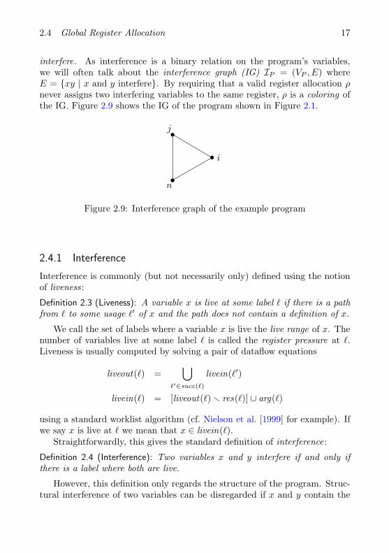
interfere. As interference is a binary relation on the program’s variables,we will often talk about the interference graph (IG) IP = (VP , E) whereE = {xy | x and y interfere}. By requiring that a valid register allocation ρnever assigns two interfering variables to the same register, ρ is a coloring ofthe IG. Figure 2.9 shows the IG of the program shown in Figure 2.1.
i
j
n
Figure 2.9: Interference graph of the example program
2.4.1 Interference
Interference is commonly (but not necessarily only) defined using the notionof liveness:
Definition 2.3 (Liveness): A variable x is live at some label ` if there is a pathfrom ` to some usage `′ of x and the path does not contain a definition of x.
We call the set of labels where a variable x is live the live range of x. Thenumber of variables live at some label ` is called the register pressure at `.Liveness is usually computed by solving a pair of dataflow equations
liveout(`) =⋃
`′∈succ(`)
livein(`′)
livein(`) = [liveout(`) r res(`)] ∪ arg(`)
using a standard worklist algorithm (cf. Nielson et al. [1999] for example). Ifwe say x is live at ` we mean that x ∈ livein(`).
Straightforwardly, this gives the standard definition of interference:
Definition 2.4 (Interference): Two variables x and y interfere if and only ifthere is a label where both are live.
However, this definition only regards the structure of the program. Struc-tural interference of two variables can be disregarded if x and y contain the
18 Foundations
start : · · ·
`1 : a← · · · `2 : b← · · ·
`3 : · · ·
`4 : · · · ← b `5 : · · · ← a
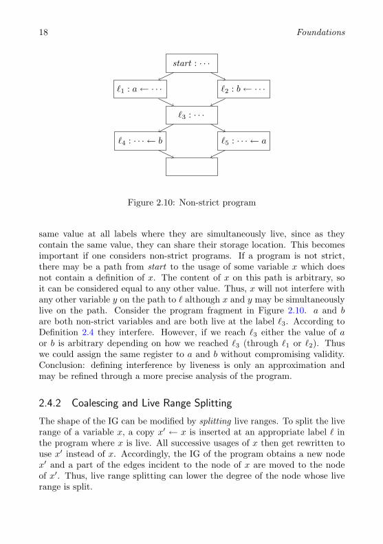
Figure 2.10: Non-strict program
same value at all labels where they are simultaneously live, since as theycontain the same value, they can share their storage location. This becomesimportant if one considers non-strict programs. If a program is not strict,there may be a path from start to the usage of some variable x which doesnot contain a definition of x. The content of x on this path is arbitrary, soit can be considered equal to any other value. Thus, x will not interfere withany other variable y on the path to ` although x and y may be simultaneouslylive on the path. Consider the program fragment in Figure 2.10. a and bare both non-strict variables and are both live at the label `3. According toDefinition 2.4 they interfere. However, if we reach `3 either the value of aor b is arbitrary depending on how we reached `3 (through `1 or `2). Thuswe could assign the same register to a and b without compromising validity.Conclusion: defining interference by liveness is only an approximation andmay be refined through a more precise analysis of the program.
2.4.2 Coalescing and Live Range Splitting
The shape of the IG can be modified by splitting live ranges. To split the liverange of a variable x, a copy x′ ← x is inserted at an appropriate label ` inthe program where x is live. All successive usages of x then get rewritten touse x′ instead of x. Accordingly, the IG of the program obtains a new nodex′ and a part of the edges incident to the node of x are moved to the nodeof x′. Thus, live range splitting can lower the degree of the node whose liverange is split.
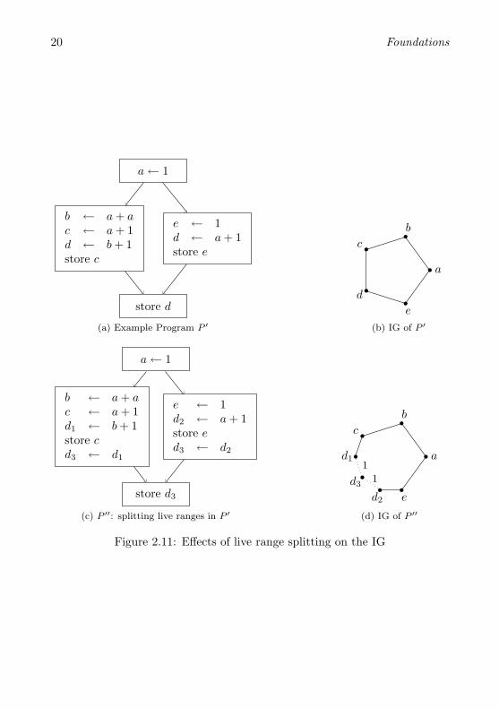
2.4 Global Register Allocation 19
Figure 2.11 shows an example program P ′, its IG and a program P ′′ whichresulted from P ′ by splitting the live range of variable d before the last basicblock. IP ′′ has a lower chromatic number (2) than IP ′ whose chromaticnumber is 3. Thus, live range splitting can have a positive effect on thecolorability of the interference graph. Consider the extreme case where thelive ranges of all live variables are split in front and behind each label. Then,the IG degenerates into a set of independent cliques where each clique consistsof the nodes corresponding to the variables live at that label. Each of thesecliques is trivially colorable using exactly as many colors as the size of theclique.
Note that constructing the SSA form breaks live ranges since Φ-operationsrepresent (parallel) copy instructions. The effect of this particular splitting onthe IG of the program will be thoroughly discussed in Chapter 4. Live rangesplitting obviously can improve the colorability of the IG, but it introduces anextensive amount of shuffle code, mainly copy instructions that transport thecontents of the split variable to new variables. As one is usually not willingto accept an arbitrary amount of inserted shuffle code, the register allocatortries to remove as many of the inserted copies as possible. This technique isknown as coalescing . The art of coalescing is to remove as many moves aspossible without pushing the chromatic number of the IG over the number ofregister available.
To express the information of variables emerging from split live ranges,we extend the IG of a program P with a set A ⊆ [VP ]2 of affinity edges (seeAppendix A for notation): xy ∈ A indicates that x and y are involved in acopy instruction and assigning x and y the same color or merging them intoone node will save a copy instruction. Furthermore, we also equip the IG witha cost function c : A→ N to weight the affinity edges arbitrarily . Thus, theIG will from now on be a quadruple IP = (VP , E, A, c). In drawings of theIG such as in Figure 2.11d, we indicate affinity edges with dotted edges andcosts superscripted.
2.4.3 Spilling
Not every program P has a valid register allocation. This is exactly the caseif the chromatic number of the interference graph is larger than the numberof available registers: χ(IP ) > |R| = k. In order to make IP k-colorable,the program must be transformed. This is achieved by writing the values ofsome set of variables to memory at some points of the program. By insertingload and store instructions for a variable x, the live range of x is fragmented.This lowers the register pressure at several other labels. The quality of the
20 Foundations
a← 1
b ← a + ac ← a + 1d ← b + 1store c
e ← 1d ← a + 1store e
store d
(a) Example Program P ′
a
b
c
d
e
(b) IG of P ′
a← 1
b ← a + ac ← a + 1d1 ← b + 1store cd3 ← d1
e ← 1d2 ← a + 1store ed3 ← d2
store d3
(c) P ′′: splitting live ranges in P ′
1
1a
b
c
d1
d3
d2 e
(d) IG of P ′′
Figure 2.11: Effects of live range splitting on the IG
2.4 Global Register Allocation 21
spilling process is crucial for the performance of the program, since the time foraccessing a memory location can exceed the time for accessing a register by atleast one order of magnitude in today’s processor architectures. An alternativeto storing and loading a variable is to recompute it. This is commonly knownas rematerialisation. Of course, all operands of the instruction writing to thevariable must be live at the point of rematerialisation. Thus, this techniqueis useful for operations with few or even no operands, such as constants.
2.4.4 Register Targeting
Up to now we assumed that each register is assignable to every variable.When compiling for real processor architectures this is rarely the case. Mostprocessors impose register constraints on several of their instructions. Thismay even lead to unallocatable programs in the first place. Assume twovariables x and y being defined by some instruction i at labels `1 and `2respectively. The instruction i has the constraint that its result is alwayswritten to a specific register. If x and y interfere, the interference graph of theprogram does not have a valid coloring since two interfering variables must beassigned the same register. Generally, one splits the live ranges of constrainedvariables at the labels where the instruction imposing the constraint is actingon the variable. This allows for moving the variable from/to the constrainedregister and place it in an arbitrary register. Common constraints of currentprocessor architectures and runtime systems are:
• An instruction requires an operand or a result to reside in a specificsubset of registers. Mostly, this subset is of size 1. We write x|S toexpress that x’s value has to be in one of the registers of the set S atits occurrence.
• The instruction requires an operand to have the same register as a result.This is commonly the case for two-address-code machines like x86.
• An instruction needs a result register to be different from some operandregister. This situation also occurs with two-address-code machines andsome RISC architectures like the ARM.
22 Foundations
3 State of the Art
The major distinction between register allocation approaches is global versuslocal register allocation. Global register allocation works at the procedurelevel, whereas local register allocation only considers basic blocks or onlysingle statements and their expression trees. Local register allocation is farless complex since it avoids all subtleties which arise from control flow split-and merge points. The drawback however is, that the local allocations haveto be combined across basic block borders. Very simple approaches store allvariables live at the end of a basic block to memory and reload all variableslive at the entrance to the successor. This approach is nowadays consideredunacceptable due to significant performance drawbacks arising from the hugeamount of memory traffic on block borders.
This problem becomes even worse when register allocation only considersa single expression tree. Although an optimal allocation for the tree can beobtained efficiently (cf. Sethi and Ullman [1970]) for standard register files,combining the allocation for each expression to acceptable fast code is diffi-cult. This problem is attacked by global register allocation which performs theallocation on the procedure level. Some compilers rely on a mixed local/globalallocation strategy reserving some registers for a local allocator inside the in-struction selector and using a global allocator to assign registers to variablesliving over multiple basic blocks.
Although global register allocation eliminates inter-block fixup-code, theproblem is algorithmically complex. Furthermore, common global registerallocators as presented in this chapter rely on heavy-weight data structuresthat need careful engineering.
The register allocation approach presented in this thesis certainly belongsto the “global” category. Thus, we will focus on global register allocationtechniques and mention other approaches along the way. The most prominenttechnique for global register allocation is graph coloring where the interfer-ence graph is materialized as a data structure and processed using coloringalgorithms.
23
24 State of the Art
3.1 Graph-Coloring Register Allocation
Graph coloring register allocation (GCRA) goes back to the 1960s whereErshov [1965] used “conflict matrices” to record interferences between vari-ables in a basic block. These matrices are basically the adjacency matrices ofthe interference graph. The breakthrough of GCRA is marked by the sem-inal work of Chaitin et al. [1981] rediscovering a coloring scheme by Kempe[1879]. Chaitin et al. proved that each undirected graph is the interferencegraph of some program. This assertion is very strong since it implies the NP-completeness of GCRA via the NP-completeness of general graph coloring(cf. [Garey and Johnson, 1979, Problem GT4]).
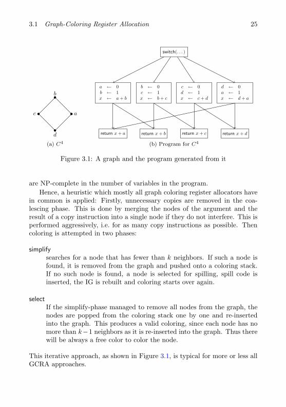
Let us revisit Chaitin’s proof since we will use a similar technique for ourpurposes in Section 4.5. Consider an arbitrary, undirected graph G = (V,E).Firstly, we augment V with an additional node, say x, giving V ′. We insertedges from x to all nodes in V resulting in a new edge set E′. An optimalcoloring for G′ = (V ′, E′) can be easily turned into a coloring for G by simplydeleting x. Since x is adjacent to all nodes in V , its color is different from thecolors assigned to the nodes in V . Now, a program is constructed from G′ inthe following way:
1. Add a start basic block S.
2. For each v ∈ V ′ add a basic block Bv containing the instruction return x+v
3. For each edge e = ab ∈ E′ add a basic block Bab containing the followinginstruction sequence:
a ← 1b ← 0x ← a + b
4. Add control flow edges from S to Bab, from Bab to Ba and Bb.
Consider figure 3.1. It shows the graph C4 and the program which is con-structed following the rules above. A valid register allocation for the programin figure 3.1b can be transformed into a valid coloring of the graph in fig-ure 3.1a simply by deleting the node for x and all its incident edges from theinterference graph of the program. Thus, not only the allocation problem butalso the problems
1. How many registers will be needed for a particular program?
2. Are k registers sufficient for a register allocation of a program?
3.1 Graph-Coloring Register Allocation 25
a
b
c
d
(a) C4
switch(. . . )
a ← 0b ← 1x ← a + b
return x + a
b ← 0c ← 1x ← b + c
return x + b
c ← 0d ← 1x ← c + d
return x + c
d ← 0a ← 1x ← d + a
return x + d
(b) Program for C4
Figure 3.1: A graph and the program generated from it
are NP-complete in the number of variables in the program.Hence, a heuristic which mostly all graph coloring register allocators have
in common is applied: Firstly, unnecessary copies are removed in the coa-lescing phase. This is done by merging the nodes of the argument and theresult of a copy instruction into a single node if they do not interfere. This isperformed aggressively, i.e. for as many copy instructions as possible. Thencoloring is attempted in two phases:
simplifysearches for a node that has fewer than k neighbors. If such a node isfound, it is removed from the graph and pushed onto a coloring stack.If no such node is found, a node is selected for spilling, spill code isinserted, the IG is rebuilt and coloring starts over again.
selectIf the simplify-phase managed to remove all nodes from the graph, thenodes are popped from the coloring stack one by one and re-insertedinto the graph. This produces a valid coloring, since each node has nomore than k−1 neighbors as it is re-inserted into the graph. Thus therewill be always a free color to color the node.
This iterative approach, as shown in Figure 3.1, is typical for more or less allGCRA approaches.
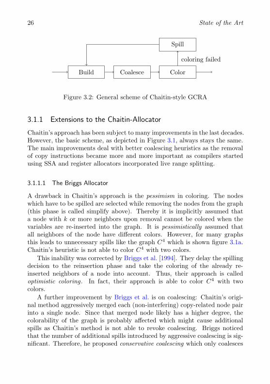
26 State of the Art
Build Coalesce Color
Spill
coloring failed
Figure 3.2: General scheme of Chaitin-style GCRA
3.1.1 Extensions to the Chaitin-Allocator
Chaitin’s approach has been subject to many improvements in the last decades.However, the basic scheme, as depicted in Figure 3.1, always stays the same.The main improvements deal with better coalescing heuristics as the removalof copy instructions became more and more important as compilers startedusing SSA and register allocators incorporated live range splitting.
3.1.1.1 The Briggs Allocator
A drawback in Chaitin’s approach is the pessimism in coloring. The nodeswhich have to be spilled are selected while removing the nodes from the graph(this phase is called simplify above). Thereby it is implicitly assumed thata node with k or more neighbors upon removal cannot be colored when thevariables are re-inserted into the graph. It is pessimistically assumed thatall neighbors of the node have different colors. However, for many graphsthis leads to unnecessary spills like the graph C4 which is shown figure 3.1a.Chaitin’s heuristic is not able to color C4 with two colors.
This inability was corrected by Briggs et al. [1994]. They delay the spillingdecision to the reinsertion phase and take the coloring of the already re-inserted neighbors of a node into account. Thus, their approach is calledoptimistic coloring . In fact, their approach is able to color C4 with twocolors.
A further improvement by Briggs et al. is on coalescing: Chaitin’s origi-nal method aggressively merged each (non-interfering) copy-related node pairinto a single node. Since that merged node likely has a higher degree, thecolorability of the graph is probably affected which might cause additionalspills as Chaitin’s method is not able to revoke coalescing. Briggs noticedthat the number of additional spills introduced by aggressive coalescing is sig-nificant. Therefore, he proposed conservative coalescing which only coalesces
3.1 Graph-Coloring Register Allocation 27
two nodes if the colorability of the graph is not affected. Thus, coalescing twonodes conservatively will never cause an additional spill.
More precisely, two nodes a and b are conservatively coalesceable if thenode c, resulting from merging a and b, will have fewer than k neighbors ofsignificant degree. The degree of a node is significant if it is larger than orequal to k. The reason for this is that all neighbors of c not of significantdegree can be removed before c is removed. Then, c surely can be removedsince there are at most k − 1 nodes which could not have been removed yet.
3.1.1.2 Iterated Register Coalescing
George and Appel [1996] extended Briggs’ approach by firstly sharpeningthe conservative coalescing criterion and secondly interleaving simplificationwith coalescing. Consider a pair of copy-related nodes a, b in the IG of someprogram. The nodes a and b can be coalesced, if each neighbor t of aeither already interferes with b, or t is of insignificant degree. For a proofconsult Appel and Palsberg [2002] for example.
Using this criterion, George and Appel [1996] modified the coloring schemeof Briggs by interleaving coalescing and simplification in the following way:
SimplifyRemove non-copy-related nodes with insignificant degree from the graph
CoalescePerform conservative coalescing on the graph resulting from simplifica-tion. The hope is that simplification already decreased the degrees ofmany nodes so that it is more likely that the criterion discussed abovematches. When there remains no pair of nodes to coalesce, simplificationis tried again.
FreezeIf the simplification/coalesce cycle could not eliminate/coalesce nodesfrom the graph, all nodes of insignificant degree which are still involvedin copies are marked as not copy-related which excludes them fromfurther coalescing attempts. These copies will be present in the resultingprogram. If a node was frozen, simplify/coalesce is resumed. Else, theallocator continues as the one of Briggs.
3.1.1.3 Optimistic Coalescing
Recognizing that conservative coalescing removes too few copies, Park andMoon [2004] revived the aggressive coalescing scheme as used in Chaitin’s
28 State of the Art
original allocator. However, their allocator is able to undo the coalescingdecision during the select phase. Assume a node a resulted from coalescingseveral nodes a1, . . . , an. If a cannot be assigned a color in the select phase,the coalescing is undone. Then each of the ai is inspected if it can be colored.If not, it is selected for spilling. For the remaining set A of not spilled nodes,each combination of subsets of A is checked if it can be colored with the samecolor. Each such subset S is rated by the spill costs all nodes in A r S wouldcause. The subset causing the least spill costs is then chosen and colored. Theremaining nodes are merged again and placed at the bottom of the coloringstack.
3.1.2 Splitting-Based Approaches
As shown in Section 2.4.2, splitting live ranges can have a positive impacton the colorability of the IG. This was firstly noticed by Fabri [1979] in amore general paper about storage optimization. Since then, there have beenmany attempts to integrate live range splitting in existing register allocatorsor build new algorithms having a live range splitting mechanism built-in.
3.1.2.1 Priority-Based Register Allocation
Based on Fabri’s observations, Chow and Hennessy [1984, 1990] presenteda graph coloring approach that differs from the Chaitin-style allocators invarious ways:
1. Register allocation is performed only on a subset of the registers. Apart of the register file are reserved for the allocation process inside theinstruction selector. Thus, this approach can be considered as a mixedlocal/global method.
2. Instead of considering the definitions and usages of variables at the in-struction level, basic blocks are used as the basic unit of allocation.A basic block is considered a single instruction and each variable de-fined/used inside the block is automatically used/defined by the block.This leads to significant smaller IGs, but it disallows a register to holddifferent quantities inside a single basic blocks which restricts the free-dom of allocation. To ease this problem, basic blocks are split after acertain number of instructions.
3. Live ranges whose nodes are of insignificant degree are removed from thegraph before starting. Thus, the algorithm only works on the criticalpart of the graph.
3.1 Graph-Coloring Register Allocation 29
4. Coloring does not follow the simplify/select-scheme but a priority-basedscheme. Live ranges with higher priorities get colored earlier. Thepriority represents the savings from assigning a live range to a registerinstead of keeping it in memory. If a live range cannot be colored itis attempted to split it. The basic block containing a definition of thelive range is inspected for a free register to contain a portion of thelive range. If there is a free register to contain the split live range, thesuccessor blocks are tried in breadth-first order.
3.1.2.2 Live Range Splitting in Chaitin-style Allocators
For Chaitin-style allocators live range splitting has a significant impact. Asthe coloring heuristic is very dependent on the degrees of the nodes in theIG, reducing the degree of a node generally results in better colorability. Re-consider the extreme example of Section 2.4.2. If the IG is decomposed intocliques and is k-colorable, i.e. there is no clique larger than k, each node hasat most k− 1 neighbors. Thus, all nodes have insignificant degree and can beeliminated by the simplify-phase.
Briggs [1992] intensively experimented with splitting live ranges beforestarting the allocation. In his PhD thesis, he mentions several split paradigms.Amongst others, he used the split points caused by Φ-operations which wereleft over after destructing SSA. His results were mixed. As colorability ofthe IG improved, his coalescing method was less able to remove a satisfactorynumber of copies. Recall that in his conservative coalescing scheme, two nodeswere only coalesced if the resulting node will have fewer than k neighbors ofsignificant degree.
3.1.3 Region-Based Approaches
Region-based register allocation performs the allocation on smaller parts, so-called regions of the program and combines the partial results to a single onefor the program. Considering regions enables the allocator to invest moreefforts in special parts of the program such as loops. A major drawback inthe general graph-coloring approaches is that the structure of the program isnot well represented by the interference graph: a node in the IG representinga “hot” variable inside a loop is hardly discriminable from some temporarywhich is used only once outside all the loops. Region based approaches mainlydiffer in the way they define a region.
Callahan and Koblenz [1991] compute a tile tree over the CFG that issimilar to the CFG part of the abstract syntax tree. The tiles are colored
30 State of the Art
separately using the standard simplify/select scheme in a bottom-up passover the tile tree. A second pass combines the results of the tile colorings intoa valid coloring for the whole program. They are furthermore able to selectgood locations for spills. By moving them up/down the tile tree, they areable to move them out of loops or inside branches. Norris and Pollock [1994]use the program dependence graph (PDG) mainly because their compilerinfrastructure is based on the PDG.
Lueh et al. [2000] provide a more general approach to region based registerallocation. First, each region is colored separately. If the IG for a region is notsimplifiable, a set of transparent live ranges (i.e. live ranges whose variablesdo not have any definition or use inside the region) is selected for spilling. Thespill is however delayed and performed in a later phase called graph fusion:The IGs of regions are fused along the control flow edges connecting theregions. If the fused IG is not simplifiable live range splitting is attempted onthe live ranges spanning the control flow edge on which fusion is attempted.In the worst case, all live ranges are split which corresponds to not fusingboth IGs. As a nice side-effect, delayed spilling regards the split live rangesand is able to spill portions of live ranges that do not contain definitions orusages of the live range’s variable.
3.1.4 Other Graph-Coloring Approaches
In the last years, the examination of the graph-theoretical structure of in-terference graphs has become of more interest in research. Andersson [2003]investigated more than 20000 IGs from existing compilers especially from theOptimal Coalescing Challenge (see Appel and George [2000] for 1-perfectness(see Section A.2) and found that all graphs he checked were 1-perfect.
Pereira and Palsberg [2005] went further and examined the interferencegraphs of the Java 1.4 standard library compiled by the JoeQ compiler afterSSA destruction and found that 95% of them were chordal. Based on thisobservation, they applied standard optimal coloring techniques for chordalgraphs like maximum cardinality search as described in Golumbic [1980].Since these coloring methods also work on non-chordal graph, although non-optimally, their allocator does not have to use the simplify/select mechanism.They furthermore present graph-based spilling and coalescing heuristics whichallow them to get rid of the iterative approach commonly found in GCRA:after spilling, coloring and coalescing the allocation is finished. This allowsfor very fast allocation, since the IG has to be built only once.
Independently and simultaneously, Brisk et al. [2005], Bouchez et al. [2005]and ourselves (see Hack [2005]) proved that the interference graphs of SSA-
3.1 Graph-Coloring Register Allocation 31
form programs are chordal. Brisk et al. are pursuing the application of SSA-based register allocation to hardware synthesis where SSA never has to bedestructed since Φ-operations are implementable with multiplexers. Bouchezet al. give a thorough complexity analysis of the spilling problem for SSA-form programs, showing the NP-completeness of several problem variants.Our consequence of the fact that SSA IGs are chordal is presented in thisthesis. Parts of this thesis have been published by the author and others inHack et al. [2005], Hack et al. [2006] and Hack and Goos [2006].
3.1.5 Practical Considerations
3.1.5.1 Register Targeting in Chaitin-style Allocators
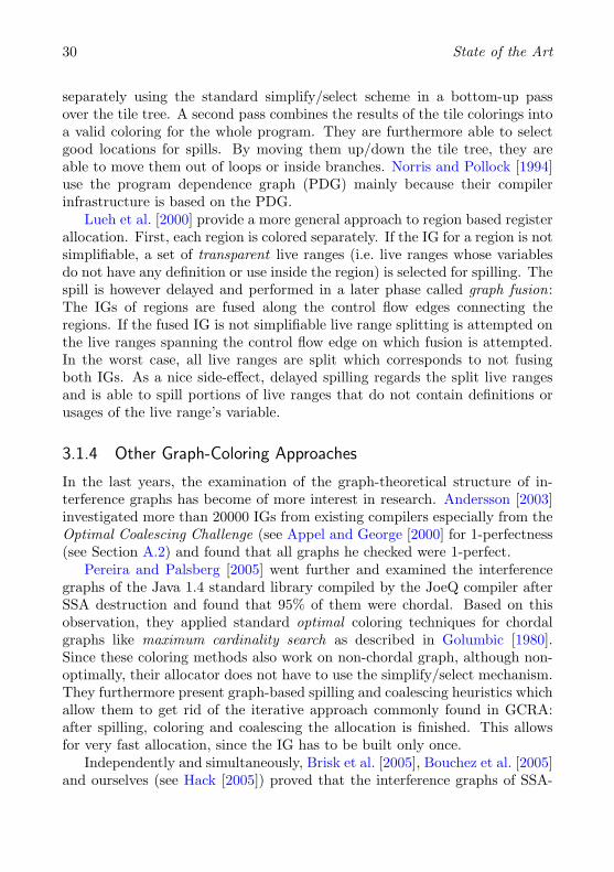
A common practice in research is to assume that each variable can be assignedevery register. For real-life processor architectures and runtime systems thisassumption is not true. Both constrain the set of assignable registers availableto the variables of the program. It might even occur that these constraintslead to an unallocatable program if a standard GCRA is applied withoutspecial preparation. This is the case if two interfering variables must residein the same register due to targeting constraints. Consider Figure 3.3a. Thevariables x and y must be both assigned to register R to fulfill the constraintsimposed by τ . Since both interfere, they cannot reside in the same register andthe constraints are not fulfillable. Instead of constraining x and y one insertscopies of both and rewrites the usages accordingly. Then, the constrained liverange is reduced to its minimum size and the interference of constrained liveranges is removed. A similar problem arises if the same variable is used atleast twice in the presence of disjunct constraints. Commonly GCRAs insertcopies behind/before each constrained definition/usage of a variable.
To express the register restriction, the IG is commonly enriched with pre-colored nodes, one for each register. If a variable cannot be assigned to registerRi, an edge from v’s node to Ri’s node is inserted. As a lot of constraints areof the type: instruction I writes its result always in register Ri thus variablev, as being the result of I, is pinned to register Ri. This introduces edgesfrom v’s node to all register nodes except the one of Ri.
Smith et al. [2004] propose an approach modifying the simplification crite-rion of the Chaitin/Briggs-allocators to handle aliased registers1 as they occurin several architectures.
1Some parts of a register can be accessed under different names. For example, bits 0-7and 8-15 of the 32-bit register eax on the x86-Architecture can be accessed with registersal and ah respectively.
32 State of the Art
x ← · · ·y ← · · ·
...· · · ← τ(x|{R}, . . . )
...· · · ← τ(y|{R}, . . . )(a) An uncolorable
Program
x ← · · ·y ← · · ·
...x′ ← x· · · ← τ(x′|{R}, . . . )
...y′ ← y· · · ← τ(y|{R}, . . . )(b) Fixed Program
Figure 3.3: A program uncolorable due to register constraints
3.1.5.2 Pre-Allocation Spilling
The spilling approach of Chaitin-style allocators is very crude since the spillingdecisions are only taken based on the coloring heuristic becoming stuck. As anode in the IG corresponds to a live range and the whole live range is selectedto be spilled, all uses and definitions are rewritten using loads and stores.However, it is not acceptable in practice to have a whole live range with fiveuses inside a loop spilled because of one use in a non-loop region of a programwhere the register pressure is too high. Region-based approaches, as presentedin the last paragraphs, try to attack this problem. In practice however, oneoften uses a spilling phase before starting the allocation (see Paleczny et al.[2001] or Morgan [1998]).
This re-allocation spilling phase lowers the register pressure at each labelto the number of available registers. This will not guarantee the allocation tosucceed without spilling but does the major amount of spilling in advance. Allspills in the allocator are then due to control flow effects or the imperfectionof the coloring heuristic. The pre-allocation spiller can be program sensitive.Morgan [1998] depicts the following procedure:
1. Before spilling some variable, determine all loops where register pressureis too high and select variables live through these loops without beingused inside of them to be spilled around the loop.
2. If this did not lower the register pressure to k everywhere, performBelady’s algorithm (see Belady [1966]) on the basic blocks where the
3.2 Other Global Approaches 33
register pressure is still too high. This algorithm was originally devel-oped for paging strategies in operating systems, selecting those pagesto be removed from main memory whose next use was furthest in thefuture. In terms of register allocation this means that if all registers areoccupied and a register is needed for a result or argument of a label,all variables currently in registers are examined and the one with thefurthest use is selected to be spilled.
This has been transferred to register allocation: if a variable has to bespilled, the one whose next use is furthest away is taken.
3. Belady’s algorithm will incur fixup loads and stores on the incomingcontrol flow edges of the block it is performed on. Attempts are madeto move these loads and stores to better places using techniques similarto partial redundancy elimination.
3.1.5.3 Storing the Interference Graph
All graph coloring approaches presented above need the IG as a data structurematerialized in memory. As interference graphs can have more than 10000nodes and are not sparse, they consume a significant amount of memoryand are time-consuming to build. Unfortunately, GCRA approaches needto perform neighbor checks (is a a neighbor of b) and the iteration over allneighbors of a node. So, an adjacency matrix or adjacency lists would bedesirable to perform both operations in acceptable time. Cooper et al. [1998]discuss engineering aspects of IGs in greater detail.
3.2 Other Global Approaches
Graph coloring has not been the only attempt to global register allocation.The costly iterative algorithm of the Chaitin-style allocators with the hugeIG as a data structure make graph coloring a technique which is not trivial toimplement, requires careful engineering and consumes a lot of compile time.Especially for the field of Just-In-Time (JIT) compilation where compile timematters, register allocation algorithms with emphasis on fast compile timehave been developed. They mostly work linearly in the size of the programand usually do not achieve the same quality as graph-coloring register allo-cators. Besides these fast algorithms, there are approaches which focus onobtaining optimal solutions for the register allcoation problem using integer
34 State of the Art
linear programming. Here, we shortly outline representative approaches forboth fields.
3.2.1 Linear-Scan
The linear-scan approach (cf. Poletto and Sarkar [1999]) aims at fast compiletimes which are of great importance in the field of JIT compilation. Unlikethe other approaches presented on the last pages, the linear-scan algorithmdoes not consider the control flow graph and precise liveness information dur-ing register allocation. It assumes that there exists a total order < of theinstructions. Using this total order, each variable has exactly one live inter-val [i, j] with i < j. These intervals can be computed by a single pass overprogram. However, since the instructions must be ordered linearly the liveintervals may cover instructions where the variable is not live according toliveness analysis (as presented in Definition 2.3).
Then, the intervals are sorted increasingly in order of their start points.In a second pass, registers are assigned first come first served to the intervals.When there is no register left to assign, one of the currently “active” intervalshas to be spilled. Different heuristics are applicable there. The one chosen byPoletto and Sarkar [1999] is to spill the interval whose end point is furthestaway which is similar to the heuristic presented in Section 3.1.5.2.
Linear-scan is very popular in JIT-compilers mainly because it runs fastand is easy to implement. Due to its simplicity and the imprecise livenessinformation the quality of the allocation is considered inferior to the oneproduced by GCRA. In the last years, several improvements were proposed tocope with the deficiencies of imprecise liveness information and incorporatingother register allocation tasks such as constraint handling and coalescing.For more details, see Traub et al. [1998], Wimmer and Mossenbock [2005] orMossenbock and Pfeiffer [2002].
3.2.2 ILP-based Approaches
Goodwin and Wilken [1996], Fu and Wilken [2002] were the first to give anILP (integer linear programming) formulation of the whole register allocationproblem including spilling, rematerialisation, live range splitting, coalescingand register targeting. Their measurements show that it takes about fiveseconds for 97% of the SPEC92 benchmark suite to be within 1% of theoptimal solution. They furthermore present a hybrid framework where criticalcontrol flow paths can be allocated with the ILP mechanism and the rest isprocessed with a standard graph coloring approach.
3.3 SSA Destruction 35
Appel and George [2001] focus on spilling and separate spilling and registerassignment. First, ILP-based spilling inserts spills and reloads and lowers theregister pressure to the number of available registers. To obtain a valid allo-cation, live ranges are split in front of each label as discussed in Section 2.4.2by inserting parallel copy instructions. Thus, the IG degenerates into a setof cliques which is trivially colorable. Now, it is up to the coalescing phaseto remove as many copies as necessary. Appel and George state this problemas finding a coloring of the IG which has minimal copy costs and name itOptimal Register Coalescing. In their experiments, they first tried iteratedregister coalescing which failed to remove a satisfactory number of copies dueto its conservatism. Second, they applied optimistic register coalescing whichproduced satisfactory results concerning the runtime of the program.
3.3 SSA Destruction
Although not being a register allocation approach SSA destruction has a sig-nificant influence on register allocation. It is common sense to destruct SSAbefore performing register allocation. This is mostly due to a historical rea-son: graph coloring register allocation was invented earlier than SSA. Tomake SSA-based compilers “compatible” with existent (non-SSA) backends,SSA has to be destructed before the code generation process starts.
As discussed in Section 2.4.2, Φ-operations induce a live range splittingon the program. Recent SSA destruction approaches which go beyond thesimple copy insertion scheme as presented in Section 2.3.3, try to subsumeas many variables of the same Φ-congruence class in the same non-SSA vari-able (see Sreedhar et al. [1999] and Rastello et al. [2004]). Thereby, theseapproaches perform a coalescing on SSA variables before register allocationand might accidentally increase the chromatic number of the graph as shownin Figure 2.11. The fact that many variables were merged into one is invisibleto the register allocator afterwards. It thus will be unable to undo this pre-allocation coalescing. To our knowledge, there is no register pressure sensitiveSSA destruction approach.
3.4 Conclusions
We presented an overview over existing approaches in global register alloca-tion which are relevant to this thesis. The salient approach is graph coloringas invented by Chaitin and improved by Briggs. The algorithm is dominated

36 State of the Art
by the generality of the occurring interference graphs; as shown in Section 3.1,each undirected graph can occur as an IG. Thus, the coloring scheme is de-signed to handle arbitrary graphs. However, the simplify/select-scheme favorsgraphs which contain some nodes of insignificant degree and eliminating anode causes more and more nodes to become eliminable.
We have seen that live range splitting is important since it renders the IGbetter colorable by the simplify/select-scheme at the costs of introducing copyinstructions which have to be eliminated using coalescing. As many compil-ers use the SSA-form at least in some optimizations, the copy instructionsintroduced by the SSA destruction are still present in the register allocationphase. This led to an increasing importance of coalescing which culminatedin the optimistic approach by Park and Moon.
4 SSA Register Allocation
4.1 Liveness, Interference and SSA
In this section, we investigate the properties of interference in strict SSA-form programs. We show that, using liveness-based interference (as given inDefinition 2.4), the interference graphs of SSA-form programs are chordal.Before turning to the discussion of liveness and interference, let us start witha remark on the special variable undef.
A Short Note on undef
In Section 2.3.2, we introduced the dummy variable undef as a means to con-struct strict SSA-form programs. At each use of undef, its value is undefined.Hence, its value can be read from an arbitrary register, i.e. it does not interferewith any other variable, although it might be simultaneously live. As wereare interested in keeping the liveness-based notion of interference, we will ex-clude undef from the set of variables on which register allocation is executed.Independently from the register allocation, we can assign an arbitrary registerto undef.
4.1.1 Liveness and Φ-operations
The standard definition of liveness, as given in Definition 2.3, is based on thenotion of usage. For ordinary operations, a variable x is used at a label ` ifx ∈ arg(`). However, this is not true for Φ-operations: control flow selects asingle row out of the Φ-matrix. The variables of this row are copied to theresult variables and the rest of the operands are ignored.
Applying the liveness-based definition of interference and treating Φ-op-erations like ordinary operations would directly lead to mutual interference
37
38 SSA Register Allocation
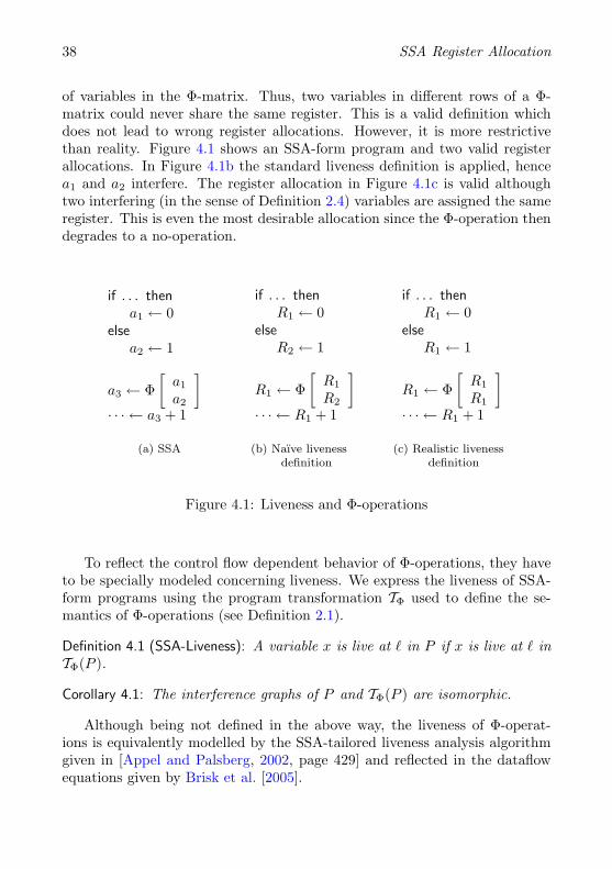
of variables in the Φ-matrix. Thus, two variables in different rows of a Φ-matrix could never share the same register. This is a valid definition whichdoes not lead to wrong register allocations. However, it is more restrictivethan reality. Figure 4.1 shows an SSA-form program and two valid registerallocations. In Figure 4.1b the standard liveness definition is applied, hencea1 and a2 interfere. The register allocation in Figure 4.1c is valid althoughtwo interfering (in the sense of Definition 2.4) variables are assigned the sameregister. This is even the most desirable allocation since the Φ-operation thendegrades to a no-operation.
if . . . thena1 ← 0
elsea2 ← 1
a3 ← Φ[
a1
a2
]· · · ← a3 + 1
(a) SSA
if . . . thenR1 ← 0
elseR2 ← 1
R1 ← Φ[
R1
R2
]· · · ← R1 + 1
(b) Naıve livenessdefinition
if . . . thenR1 ← 0
elseR1 ← 1
R1 ← Φ[
R1
R1
]· · · ← R1 + 1
(c) Realistic livenessdefinition
Figure 4.1: Liveness and Φ-operations
To reflect the control flow dependent behavior of Φ-operations, they haveto be specially modeled concerning liveness. We express the liveness of SSA-form programs using the program transformation TΦ used to define the se-mantics of Φ-operations (see Definition 2.1).
Definition 4.1 (SSA-Liveness): A variable x is live at ` in P if x is live at ` inTΦ(P ).
Corollary 4.1: The interference graphs of P and TΦ(P ) are isomorphic.
Although being not defined in the above way, the liveness of Φ-operat-ions is equivalently modelled by the SSA-tailored liveness analysis algorithmgiven in [Appel and Palsberg, 2002, page 429] and reflected in the dataflowequations given by Brisk et al. [2005].
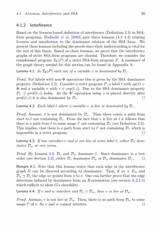
4.1 Liveness, Interference and SSA 39
4.1.2 Interference
Based on the liveness-based definition of interference (Definition 2.3) in SSA-form programs, Budimlic et al. [2002] gave three lemmas (4.2–4.4) relatingliveness and interference to the dominance relation of the SSA form. Wepresent these lemmas including the proofs since their understanding is vital forthe rest of this thesis. Based on these lemmas, we prove that the interferencegraphs of strict SSA-form programs are chordal. Therefore, we consider thetransformed program TΦ(P ) of a strict SSA-form program P . A summary ofthe graph theory needed for this section can be found in Appendix A.
Lemma 4.1: In TΦ(P ) each use of a variable v is dominated by Dv.
Proof. For labels with non-Φ operations this is given by the SSA dominanceproperty (Definition 2.2). Consider a strict program P , a label ` with op(`) =Φ and a variable v with v ∈ arg(`, i). Due to the SSA dominance propertyDv � pred(`, i) holds. As the Φr-operation using v is placed directly afterpred(`, i) it is also dominated by Dv.
Lemma 4.2: Each label ` where a variable v is live is dominated by Dv.
Proof. Assume, ` is not dominated by Dv. Then there exists a path fromstart to ` not containing Dv. From the fact that v is live at ` it follows thatthere is a path from ` to some usage `′ not containing Dv (see Definition 2.3).This implies, that there is a path from start to `′ not containing Dv which isimpossible in a strict program.
Lemma 4.3: If two variables v and w are live at some label `, either Dv dom-inates Dw or vice versa.
Proof. By Lemma 4.2, Dv and Dw dominate `. Since dominance is a treeorder (see Section 2.2), either Dv dominates Dw or Dw dominates Dv.
Remark 4.1: Note that this lemma states that each edge in the interferencegraph G can be directed according to dominance. Thus, if uv ∈ EG andDu � Dv the edge uv points from u to v. One can further prove that the edgedirections induced by dominance form an R-orientation (see section A.2.1.4)which suffices to show G’s chordality.
Lemma 4.4: If v and w interfere and Dv � Dw, then v is live at Dw.
Proof. Assume, v is not live at Dw. Then, there is no path from Dw to someusage `′ of v. So v and w cannot interfere.
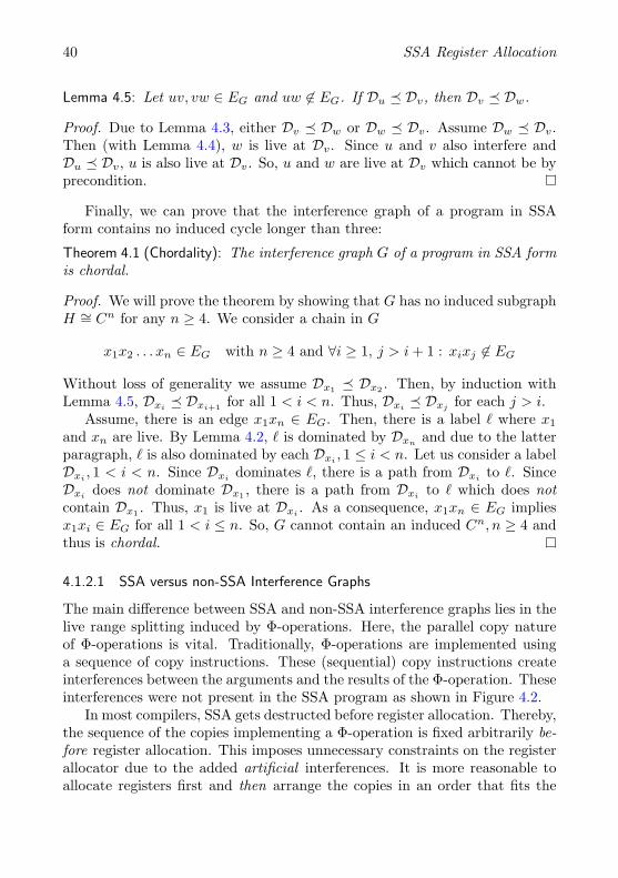
40 SSA Register Allocation
Lemma 4.5: Let uv, vw ∈ EG and uw 6∈ EG. If Du � Dv, then Dv � Dw.
Proof. Due to Lemma 4.3, either Dv � Dw or Dw � Dv. Assume Dw � Dv.Then (with Lemma 4.4), w is live at Dv. Since u and v also interfere andDu � Dv, u is also live at Dv. So, u and w are live at Dv which cannot be byprecondition.
Finally, we can prove that the interference graph of a program in SSAform contains no induced cycle longer than three:
Theorem 4.1 (Chordality): The interference graph G of a program in SSA formis chordal.
Proof. We will prove the theorem by showing that G has no induced subgraphH ∼= Cn for any n ≥ 4. We consider a chain in G
x1x2 . . . xn ∈ EG with n ≥ 4 and ∀i ≥ 1, j > i + 1 : xixj 6∈ EG
Without loss of generality we assume Dx1 � Dx2 . Then, by induction withLemma 4.5, Dxi � Dxi+1 for all 1 < i < n. Thus, Dxi � Dxj for each j > i.
Assume, there is an edge x1xn ∈ EG. Then, there is a label ` where x1
and xn are live. By Lemma 4.2, ` is dominated by Dxn and due to the latterparagraph, ` is also dominated by each Dxi , 1 ≤ i < n. Let us consider a labelDxi , 1 < i < n. Since Dxi dominates `, there is a path from Dxi to `. SinceDxi does not dominate Dx1 , there is a path from Dxi to ` which does notcontain Dx1 . Thus, x1 is live at Dxi . As a consequence, x1xn ∈ EG impliesx1xi ∈ EG for all 1 < i ≤ n. So, G cannot contain an induced Cn, n ≥ 4 andthus is chordal.
4.1.2.1 SSA versus non-SSA Interference Graphs
The main difference between SSA and non-SSA interference graphs lies in thelive range splitting induced by Φ-operations. Here, the parallel copy natureof Φ-operations is vital. Traditionally, Φ-operations are implemented usinga sequence of copy instructions. These (sequential) copy instructions createinterferences between the arguments and the results of the Φ-operation. Theseinterferences were not present in the SSA program as shown in Figure 4.2.
In most compilers, SSA gets destructed before register allocation. Thereby,the sequence of the copies implementing a Φ-operation is fixed arbitrarily be-fore register allocation. This imposes unnecessary constraints on the registerallocator due to the added artificial interferences. It is more reasonable toallocate registers first and then arrange the copies in an order that fits the
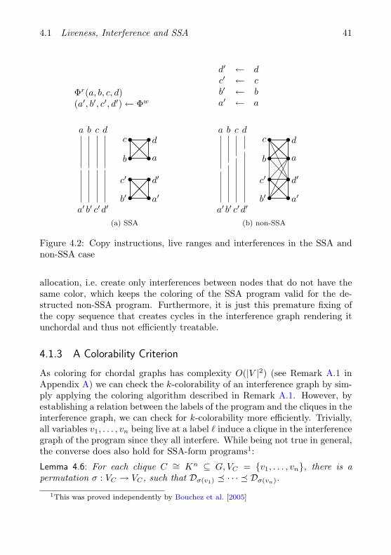
4.1 Liveness, Interference and SSA 41
Φr(a, b, c, d)(a′, b′, c′, d′)← Φw
a
a′
b
b′
c
c′
d
d′
dc
b a
d′c′
b′ a′
(a) SSA
d′ ← dc′ ← cb′ ← ba′ ← a
a
a′
b
b′
c
c′
d
d′
dc
b a
d′c′
b′ a′
(b) non-SSA
Figure 4.2: Copy instructions, live ranges and interferences in the SSA andnon-SSA case
allocation, i.e. create only interferences between nodes that do not have thesame color, which keeps the coloring of the SSA program valid for the de-structed non-SSA program. Furthermore, it is just this premature fixing ofthe copy sequence that creates cycles in the interference graph rendering itunchordal and thus not efficiently treatable.
4.1.3 A Colorability Criterion
As coloring for chordal graphs has complexity O(|V |2) (see Remark A.1 inAppendix A) we can check the k-colorability of an interference graph by sim-ply applying the coloring algorithm described in Remark A.1. However, byestablishing a relation between the labels of the program and the cliques in theinterference graph, we can check for k-colorability more efficiently. Trivially,all variables v1, . . . , vn being live at a label ` induce a clique in the interferencegraph of the program since they all interfere. While being not true in general,the converse does also hold for SSA-form programs1:
Lemma 4.6: For each clique C ∼= Kn ⊆ G, VC = {v1, . . . , vn}, there is apermutation σ : VC → VC , such that Dσ(v1) � · · · � Dσ(vn).
1This was proved independently by Bouchez et al. [2005]
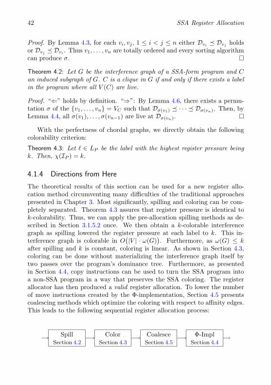
42 SSA Register Allocation
Proof. By Lemma 4.3, for each vi, vj , 1 ≤ i < j ≤ n either Dvi � Dvj holdsor Dvj � Dvi . Thus v1, . . . , vn are totally ordered and every sorting algorithmcan produce σ.
Theorem 4.2: Let G be the interference graph of a SSA-form program and Can induced subgraph of G. C is a clique in G if and only if there exists a labelin the program where all V (C) are live.
Proof. “⇐” holds by definition. “⇒”: By Lemma 4.6, there exists a permu-tation σ of the {v1, . . . , vn} = VC such that Dσ(v1) � · · · � Dσ(vn). Then, byLemma 4.4, all σ(v1), . . . , σ(vn−1) are live at Dσ(vn).
With the perfectness of chordal graphs, we directly obtain the followingcolorability criterion:
Theorem 4.3: Let ` ∈ LP be the label with the highest register pressure beingk. Then, χ(IP ) = k.
4.1.4 Directions from Here
The theoretical results of this section can be used for a new register allo-cation method circumventing many difficulties of the traditional approachespresented in Chapter 3. Most significantly, spilling and coloring can be com-pletely separated. Theorem 4.3 assures that register pressure is identical tok-colorability. Thus, we can apply the pre-allocation spilling methods as de-scribed in Section 3.1.5.2 once. We then obtain a k-colorable interferencegraph as spilling lowered the register pressure at each label to k. This in-terference graph is colorable in O
(|V | · ω(G)
). Furthermore, as ω(G) ≤ k
after spilling and k is constant, coloring is linear. As shown in Section 4.3,coloring can be done without materializing the interference graph itself bytwo passes over the program’s dominance tree. Furthermore, as presentedin Section 4.4, copy instructions can be used to turn the SSA program intoa non-SSA program in a way that preserves the SSA coloring. The registerallocator has then produced a valid register allocation. To lower the numberof move instructions created by the Φ-implementation, Section 4.5 presentscoalescing methods which optimize the coloring with respect to affinity edges.This leads to the following sequential register allocation process:
SpillSection 4.2
ColorSection 4.3
CoalesceSection 4.5
Φ-ImplSection 4.4
4.1 Liveness, Interference and SSA 43
Section 4.6 discusses how the allocator has to be modified in order to handleregister constraints imposed by the processor’s instruction set architectureand the runtime’s binary interface. This comprises an additional pass beforespilling and a slight modification to the coloring phase.
44 SSA Register Allocation
4.2 Spilling
To apply the coloring algorithm of Section 4.3 and to obtain a valid registerallocation, we need to establish that the program is k-colorable. In prac-tice, it is likely that the register pressure in a program exceeds the numberof available registers. Therefore, before coloring, spilling has to rewrite theprogram in order to make it k-colorable. This rewriting is done using load-and store-operations which transfer the values between the register file andthe main memory. As the access to main memory can be several orders ofmagnitude slower than the access to registers, load- and store-operations mustbe used very carefully. The complexity of minimizing this memory traffic hasbeen shown NP-complete by Farach and Liberatore [1998] and in particularby Bouchez et al. [2005] in the SSA context.
The failure-driven spilling of GCRAs is often not satisfactory, since theprogram’s structure is insufficiently represented in the interference graph.Hence, most compilers apply a pre-coloring spilling phase which lowers theregister pressure at the labels in the program to the amount of available regis-ters (see Section 3.1.5.2). Due to Theorem 4.3 this heuristic suffices to producea validly colorable program in the SSA-based setting.
Hence, the main focus of this section is to discuss how the existing andapproved program-sensitive spilling approaches can be applied to SSA-formprograms.
4.2.1 Spilling on SSA
Before presenting how existing techniques can be adapted to work in the SSA-based setting, we discuss several SSA specific issues a spilling algorithm hasto deal with. Let us first define what spilling means. If the register pressureis too high at a certain label, one of the variables live there cannot be heldin a register and must thus be moved to memory. Therefore, we enhancethe program with a second set of variables M = {m1, . . . } called memoryvariables. To make memory variables better distinguishable from ordinaryvariables, we typeset them in bold face. Memory variables are excluded fromregister allocation since they describe values in memory. However, each mem-ory variable must have a location in memory where its value is held. Similarlyto the map ρ which assigns each (ordinary) variable a register, we introducea map & : M → N which assigns each memory variable a memory address. Incontrast to the set of registers, we assume that there are at least as many mem-ory addresses as memory variables so that memory variables never compete
4.2 Spilling 45
for the same resource. Furthermore, we allow three operations to read/writememory variables:
1. An operation spill2 which reads an ordinary variable and writes to amemory variable.
2. An operation reload which reads a memory variable and writes to anordinary variable.
3. The Φ-operation.
All other operations must work on ordinary variables.3 A spilling algorithmhas to make sure that this condition is met by placing spill- and reload-operations at suitable places. Two aspects demand special attention and arespecific to spilling on the SSA form.
4.2.1.1 Φ-operations with Memory Operands
A Φ-operation may define more variables as registers are available. Thus, anSSA-based spiller must not only insert spill and reloads but also rewrite Φ-operations. Let k be the number of registers. After spilling, |res(`) r M | ≤ kmust hold for each label ` containing a Φ-operation.
Note carefully that a Φ-operation with memory operands may introducememory operations when the Φ-operation gets lowered by the Φ-implementationphase as described in Section 4.4.2. Whether a Φ-operation with memoryoperands causes memory traffic depends on the spill slot assignment &. Iffor each memory Φ-result y and each corresponding argument xi there is&y = &xi then no code has to be generated for the memory part of the Φ-operation at all. Thus, “optimal” spilling approaches must not only considerthe placement of spill and reload operations in order to fulfil the register pres-sure criterion but also the assignment of spill slots. To our knowledge, thisproblem has not been studied yet. Even the “optimal” approaches presentedin Section 3.2.2 ignore this fact.
We also require that if the result variable of a Φ-operation is a memoryvariable, all corresponding operands are memory variables as well. One couldalso allow having mixed memory/register operands for a result but this would
2The reason why we name these instructions spill and reload is that we want to keepthe spilling process as architecture-independent as possible. When the spiller insertedthese operations the instruction selection mechanism can turn them into actual machineinstructions.
3This reflects common load/store architectures. Some CISC machines, such as x86, havethe possibility to directly process memory operands.
46 SSA Register Allocation
defer a part of the spill and reload code insertion to the SSA destructionphase. We found it more elegant to have only the spiller handling the spilland reload code.
4.2.1.2 SSA Reconstruction
After spilling, the program must be in SSA form to benefit from the resultsof Section 4.1. However, if a variable v is reloaded at several locations, thesereloads form additional definitions of v. This clearly violates the static singleassignment property (see Figure 4.3). Therefore, for each variable v for whichreloads are introduced by the spiller, SSA has to be reconstructed.
Instead of performing an SSA construction algorithm on the whole pro-gram, we can restrict ourselves to the variables which were involved in spilling.All other variables still have only one definition.
We follow the same principles as the classical SSA construction algorithmby Cytron et al. [1991]: For each spilled variable x compute the iterateddominance frontier of the set of labels L containing the definition and alllabels containing a reload of x:
L = {` | res(`) = {x} ∧ op(`) = reload} ∪ {Dx}
Firstly, give each variable defined by the labels in L a new version number.This reinstalls the single assignment property. Secondly, we have to rewireeach use of former x to one of the variables defined at the labels in L. LetF bet the set of iterated dominance frontiers of L (for example, see [Appeland Palsberg, 2002, page 406] for an algorithm to compute these). Let U bethe set of uses of x. For each ` ∈ U we search up the dominator tree. If wereach a label `r in L, we subsitute x in arg(`) by res(`r). If ` is in the iterateddominance frontier F , we insert a Φ-operation and search the predecessors of` for valid definitions of x. Algorithm 4.1 shows this procedure in pseudo-code. Note that by re-wiring the usages of several variables, some variablesdefined by Φ-operations may not be used anymore. A dead code eliminationpass after spilling will remove these.
4.2.2 Generic Procedure
Assume some spilling algorithm produces a set of spills and reloads for somevariable y in the original program. The new program P ′ has to be rewrittento reflect the spilling algorithm’s results. Let us consider possible spills andreloads for y. Firstly, y can be the result of a Φ-operation or not. If it is,the spiller has to determine if y’s entry in the Φ-operation shall be completely
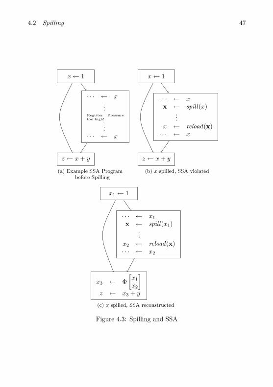
4.2 Spilling 47
x← 1
· · · ← x...
Register Pressuretoo high!
...· · · ← x
z ← x + y
(a) Example SSA Programbefore Spilling
x← 1
· · · ← xx ← spill(x)
...x ← reload(x)· · · ← x
z ← x + y
(b) x spilled, SSA violated
x1 ← 1
· · · ← x1
x ← spill(x1)...
x2 ← reload(x)· · · ← x2
x3 ← Φ[x1
x2
]z ← x3 + y
(c) x spilled, SSA reconstructed
Figure 4.3: Spilling and SSA
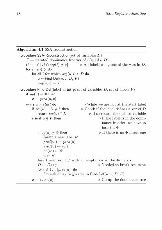
48 SSA Register Allocation
Algorithm 4.1 SSA reconstruction
procedure SSA-Reconstruction(set of variables D)F ← iterated dominance frontier of {Dd | d ∈ D}U ← {` | D ∩ arg(`) 6= ∅} . All labels using one of the vars in D.for all u ∈ U do
for all i for which arg(u, i) ∈ D dox←Find-Def(u, i, D, F )arg(u, i)← x
procedure Find-Def(label u, int p, set of variables D, set of labels F )if op(u) = Φ then
u← pred(u, p)while u 6= start do . While we are not at the start label
if res(u) ∩D 6= ∅ then . Check if the label defines a var of Dreturn res(u) ∩D . If so return the defined variable
else if u ∈ F then . If the label is in the domi-nance frontier, we have toinsert a Φ
if op(u) 6= Φ then . If there is no Φ insert oneInsert a new label u′
pred(u′)← pred(u)pred(u)← 〈u′〉op(u′)← Φu← u′
Insert new result y′ with an empty row in the Φ-matrixD ← D ∪ y′ . Needed to break recursionfor i ∈ 1 . . . |pred(u)| do
Set i-th entry in y’s row to Find-Def(u, i, D, F )u← idom(u) . Go up the dominance tree
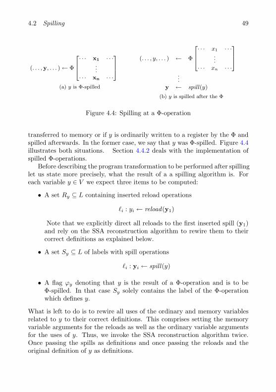
4.2 Spilling 49
(. . . ,y, . . . )← Φ
264· · · x1 · · ·...
· · · xn · · ·
375(a) y is Φ-spilled
(. . . , y, . . . ) ← Φ
264· · · x1 · · ·...
· · · xn · · ·
375...
y ← spill(y)
(b) y is spilled after the Φ
Figure 4.4: Spilling at a Φ-operation
transferred to memory or if y is ordinarily written to a register by the Φ andspilled afterwards. In the former case, we say that y was Φ-spilled. Figure 4.4illustrates both situations. Section 4.4.2 deals with the implementation ofspilled Φ-operations.
Before describing the program transformation to be performed after spillinglet us state more precisely, what the result of a a spilling algorithm is. Foreach variable y ∈ V we expect three items to be computed:
• A set Ry ⊆ L containing inserted reload operations
`i : yi ← reload(y1)
Note that we explicitly direct all reloads to the first inserted spill (y1)and rely on the SSA reconstruction algorithm to rewire them to theircorrect definitions as explained below.
• A set Sy ⊆ L of labels with spill operations
`i : yi ← spill(y)
• A flag ϕy denoting that y is the result of a Φ-operation and is to beΦ-spilled. In that case Sy solely contains the label of the Φ-operationwhich defines y.
What is left to do is to rewire all uses of the ordinary and memory variablesrelated to y to their correct definitions. This comprises setting the memoryvariable arguments for the reloads as well as the ordinary variable argumentsfor the uses of y. Thus, we invoke the SSA reconstruction algorithm twice.Once passing the spills as definitions and once passing the reloads and theoriginal definition of y as definitions.
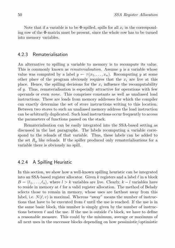
50 SSA Register Allocation
Note that if a variable is to be Φ-spilled, spills for all xi in the correspond-ing row of the Φ-matrix must be present, since the whole row has to be turnedinto memory variables.
4.2.3 Rematerialisation
An alternative to spilling a variable to memory is to recompute its value.This is commonly known as rematerialisation. Assume y is a variable whosevalue was computed by a label y ← τ(x1, . . . , xn). Recomputing y at someother place of the program obviously requires that the xi are live at thisplace. Hence, the spilling decisions for the xi influence the recomputabilityof y. Thus, rematerialisation is especially attractive for operations with fewoperands or even none. This comprises constants as well as unaliased loadinstructions. These are loads from memory addresses for which the compilercan exactly determine the set of store instructions writing to this location.Between two stores to such an unaliased memory address the load instructioncan be arbitrarily duplicated. Such load instructions occur frequently to accessthe parameters of functions passed on the stack.
Rematerialisation can be easily integrated into the SSA-based setting asdiscussed in the last paragraphs. The labels recomputing a variable corre-spond to the reloads of that variable. Thus, these labels can be added tothe set Ry like reloads. If the spiller produced only rematerialisations for avariable there is obviously no spill.
4.2.4 A Spilling Heuristic
In this section, we show how a well-known spilling heuristic can be integratedinto an SSA-based register allocator. Given k registers and a label ` in a blockB = 〈`1, . . . , `n〉, where l > k variables are live. Clearly, k − l variables haveto reside in memory at ` for a valid register allocation. The method of Beladyselects those to remain in memory, whose uses are farthest away from thislabel, i.e. N(`, v) is maximal. Whereas “away” means the number of instruc-tions that have to be executed from ` until the use is reached. If the use is inthe same basic block, this number is simply given by the number of instruc-tions between ` and the use. If the use is outside `’s block, we have to definea reasonable measure. This could by the minimum, average or maximum ofall next uses in the successor blocks depending on how pessimistic/optimistic
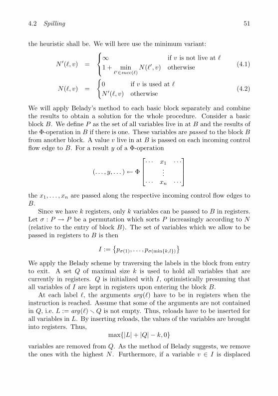
4.2 Spilling 51
the heuristic shall be. We will here use the minimum variant:
N ′(`, v) =
∞ if v is not live at `
1 + min`′∈succ(`)
N(`′, v) otherwise (4.1)
N(`, v) =
{0 if v is used at `
N ′(`, v) otherwise(4.2)
We will apply Belady’s method to each basic block separately and combinethe results to obtain a solution for the whole procedure. Consider a basicblock B. We define P as the set of all variables live in at B and the results ofthe Φ-operation in B if there is one. These variables are passed to the block Bfrom another block. A value v live in at B is passed on each incoming controlflow edge to B. For a result y of a Φ-operation
(. . . , y, . . . )← Φ
· · · x1 · · ·...
· · · xn · · ·
the x1, . . . , xn are passed along the respective incoming control flow edges toB.
Since we have k registers, only k variables can be passed to B in registers.Let σ : P → P be a permutation which sorts P increasingly according to N(relative to the entry of block B). The set of variables which we allow to bepassed in registers to B is then
I :={pσ(1), . . . , pσ(min{k,l})
}We apply the Belady scheme by traversing the labels in the block from entryto exit. A set Q of maximal size k is used to hold all variables that arecurrently in registers. Q is initialized with I, optimistically presuming thatall variables of I are kept in registers upon entering the block B.
At each label `, the arguments arg(`) have to be in registers when theinstruction is reached. Assume that some of the arguments are not containedin Q, i.e. L := arg(`) r Q is not empty. Thus, reloads have to be inserted forall variables in L. By inserting reloads, the values of the variables are broughtinto registers. Thus,
max{|L|+ |Q| − k, 0}
variables are removed from Q. As the method of Belady suggests, we removethe ones with the highest N . Furthermore, if a variable v ∈ I is displaced
52 SSA Register Allocation
before it was used, there is no sense in passing v to B in a register. inB
denotes the set of all v ∈ I which are used in B before they are displaced.We assume, that all variables defined by τ = op(`) are written to registers
upon executing τ . This means, that
max{|res(`)|+ |Q| − k, 0}
variables are displaced from Q when τ writes its results4. Note, that for allv ∈ arg(`), there is N(v, `) = 0 which implies that the arg(`) will be displacedlastly. However, it is not the uses at ` which decide but the uses after `. Thisis resembled by N ′ as defined above. We define the set outB to be the valueof Q after processing each label in the block.
Finally, after processing each block as described above, we have to combinethe results to form a valid solution for the whole program. In particular, wehave to assure, that each variable in inB for some block B must reach B ina register. Therefore, we have to check each predecessor P of B and insertreloads for all inB routP on the edge from P to B5. All the spills and reloadsdetermined by this procedure are then given to the algorithm described inSection 4.2.2 to restore the SSA property.
4Note, that Q ∩ res(`) = ∅ since the program is in SSA form.5Inserting code on an edge is possible by eliminating critical edges and placing the code
in the appropriate block.
4.3 Coloring 53
4.3 Coloring
Let us assume that the program is k-colorable, i.e. the spilling phase loweredthe register pressure to k at all labels where it exceeded k. Hence, the chro-matic number ω(G) of (chordal) interference graph G of the program is lessor equal to k. A chordal graph G can be efficiently colored in O
(|V | · ω(G)
)using perfect elimination orders (see Appendix A for the necessary graphtheory and specifically Remark A.1). The coloring process is similar to thesimplify/select-scheme presented in Section 3.1. The major difference is thata node has not only to be of insignificant degree but also simplicial6 to beremoved from the graph. Note that this is a strengthening of the criterionused in Chaitin-style allocators: if IP is k-colorable, the largest clique is ofsize k due to the perfectness of chordal graphs. All neighbors of a simplicialnode are contained in the same clique. Thus it has at most k − 1 neighborsand is of insignificant degree.
Lemma 4.5 directly leads to the fact that dominance induces a perfectelimination order on the interference graph. Assume P to be the transformedversion of an SSA-form program using TΦ and IP = (V,E, A, c).
Theorem 4.4: A variable v can be added to a PEO of IP if all variables whosedefinitions are dominated by the definition of v have been added to the PEO.
Proof. To be added to a PEO, v must be simplicial. Let us assume, v is notsimplicial. Then, by definition, there exist two neighbors a, b of v that arenot connected (va, vb ∈ E and ab 6∈ E). By proposition, all variables whosedefinitions are dominated by Dv have been added to the PEO and removedfrom IP . Thus, Da � Dv. Then, by Lemma 4.5, Dv � Db which contradictsthe proposition. Thus, v is simplicial.
Thus, we obtain a perfect elimination order on IP by a post-order traversalof the dominance tree of the program. Conversely, we can start coloring atthe label which dominates all other labels moving to the label dominatingall others but the former one and so on. Thus, coloring can be done in apre-order walk of the dominance tree as shown in Algorithm 4.2.
6i.e. all its neighbors form a clique.
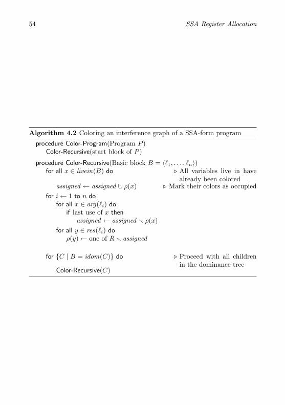
54 SSA Register Allocation
Algorithm 4.2 Coloring an interference graph of a SSA-form program
procedure Color-Program(Program P )Color-Recursive(start block of P )
procedure Color-Recursive(Basic block B = 〈`1, . . . , `n〉)for all x ∈ livein(B) do . All variables live in have
already been coloredassigned ← assigned ∪ ρ(x) . Mark their colors as occupied
for i← 1 to n dofor all x ∈ arg(`i) do
if last use of x thenassigned ← assigned r ρ(x)
for all y ∈ res(`i) doρ(y)← one of R r assigned
for {C | B = idom(C)} do . Proceed with all childrenin the dominance tree
Color-Recursive(C)
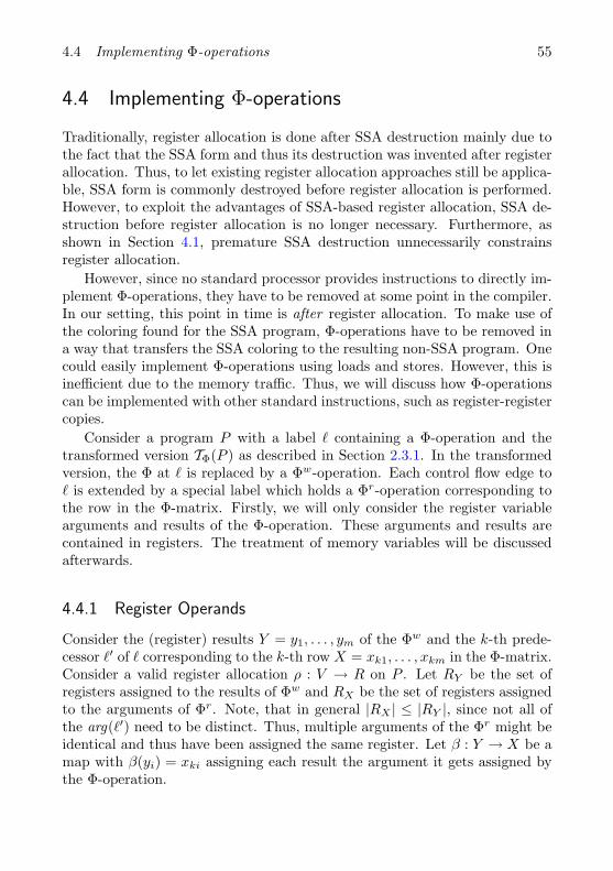
4.4 Implementing Φ-operations 55
4.4 Implementing Φ-operations
Traditionally, register allocation is done after SSA destruction mainly due tothe fact that the SSA form and thus its destruction was invented after registerallocation. Thus, to let existing register allocation approaches still be applica-ble, SSA form is commonly destroyed before register allocation is performed.However, to exploit the advantages of SSA-based register allocation, SSA de-struction before register allocation is no longer necessary. Furthermore, asshown in Section 4.1, premature SSA destruction unnecessarily constrainsregister allocation.
However, since no standard processor provides instructions to directly im-plement Φ-operations, they have to be removed at some point in the compiler.In our setting, this point in time is after register allocation. To make use ofthe coloring found for the SSA program, Φ-operations have to be removed ina way that transfers the SSA coloring to the resulting non-SSA program. Onecould easily implement Φ-operations using loads and stores. However, this isinefficient due to the memory traffic. Thus, we will discuss how Φ-operationscan be implemented with other standard instructions, such as register-registercopies.
Consider a program P with a label ` containing a Φ-operation and thetransformed version TΦ(P ) as described in Section 2.3.1. In the transformedversion, the Φ at ` is replaced by a Φw-operation. Each control flow edge to` is extended by a special label which holds a Φr-operation corresponding tothe row in the Φ-matrix. Firstly, we will only consider the register variablearguments and results of the Φ-operation. These arguments and results arecontained in registers. The treatment of memory variables will be discussedafterwards.
4.4.1 Register Operands
Consider the (register) results Y = y1, . . . , ym of the Φw and the k-th prede-cessor `′ of ` corresponding to the k-th row X = xk1, . . . , xkm in the Φ-matrix.Consider a valid register allocation ρ : V → R on P . Let RY be the set ofregisters assigned to the results of Φw and RX be the set of registers assignedto the arguments of Φr. Note, that in general |RX | ≤ |RY |, since not all ofthe arg(`′) need to be distinct. Thus, multiple arguments of the Φr might beidentical and thus have been assigned the same register. Let β : Y → X be amap with β(yi) = xki assigning each result the argument it gets assigned bythe Φ-operation.
56 SSA Register Allocation
`′ : Φr(R1, R1, R2, R5, R4)
` : (R1, R2, R3, R4, R5)← Φw
· · · ← τ(R6, . . . )
(a) Φr-Φw-pair
R1R2
R3
R4 R5
R6
(b) Register TransferGraph T
Figure 4.5: A register allocated Φw-Φr-pair and the corresponding registertransfer graphs T and T ′
Let us now consider the (directed) register transfer graph T = (R, TE).The nodes of the transfer graph are formed by the registers. The edges TE ⊆R×R represent the value transport between the registers caused by the Φ-op-eration at `: We draw an edge from Ri to Rj for each y ∈ Y with ρ(y) = Rj
and ρ(β(y)) = Ri to indicate that the value of Ri has to be moved to Rj .More formally:
TE ={(
ρ(β(y)), ρ(y))| y ∈ Y
}(4.3)
Note that each node has only one edge pointing at it since each register iswritten at most once by the Φw-instruction. However, a node might very wellhave more than one outgoing edge. This indicates that a variable is duplicatedby the Φ-operation.
Figure 4.5a shows an example for a Φw-Φr-pair and the correspondingregister transfer graph. The first two arguments of the Φr are the same asthey are kept in the same register (R1). The Φw creates a copy of the valuein R1 and stores it in R2. Hence, the node R1 in the corresponding transfergraph T (see Figure 4.5b) has two outgoing edges.
The register-register move instructions concerning T are now generated bythe following scheme:
1. First, consider the set of registers
U ={ρ(y) | y ∈ Y ∧ β(y) = undef
}which will hold a copy of the dummy variable undef (see Section 2.3.2).As their content is undefined, no move instruction has to be created toinitialize their value. Hence, all incoming edges to the nodes in U canbe deleted.
4.4 Implementing Φ-operations 57
2. Initialize a set F containing all unused registers at the label of the Φr-operation `′. Note that F is not the set of nodes in T which have noincident edges. It has to be calculated by regarding all variables live at`′ and the registers allocated to them. In our example in Figure 4.5b,R6 has no incident edges but is not in F since it is allocated to a variablewhich is live in at `.
3. While there is an edge e = (r, s), r 6= s for which the outdegree of sequals 0:The register s does not carry an argument value which has to be trans-ferred to a result. For example, the edge (R2, R3) in Figure 4.5b fulfillsthis property. Thus, we can safely write to register s by issuing a copy
s← r
Then, e is deleted from T as the move was issued. To free the registersas early as possible, we let all remaining outgoing edges of r originate ats except for self-loops. (Although it would not be incorrect to redirectself-loops, it would create unnecessary move instructions.) We add r tothe set of free registers F and remove s from F .
4. Now, T is either empty or contains one or more cycles of the formC = {(r1, r2), (r2, r2), . . . , (rn, r1)} such as the cycle (R4, R5), (R5, R4)in Figure 4.5b. Such a cycle corresponds to a permutation of registerswhich can be implemented in various ways:
(a) Trivially, self-loops (cycles of length 1) generate no instruction.(b) Assume F is not empty and contains a free register rt. Then we
can implement the cycle C by a sequence of copy instructions
rt ← r1
r1 ← r2
r2 ← r3
...rn ← rt
(c) Assume F is empty and thus there is no free register. Note thatthis is only the case if transfer graph solely consists of cycles (in-cluding self-loops) and the register pressure is at maximum at `′.As known from algebra, each permutation can be implemented us-ing a series of transpositions, in our case an instruction that swapstwo registers.
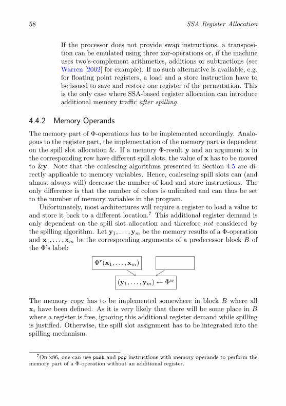
58 SSA Register Allocation
If the processor does not provide swap instructions, a transposi-tion can be emulated using three xor-operations or, if the machineuses two’s-complement arithmetics, additions or subtractions (seeWarren [2002] for example). If no such alternative is available, e.g.for floating point registers, a load and a store instruction have tobe issued to save and restore one register of the permutation. Thisis the only case where SSA-based register allocation can introduceadditional memory traffic after spilling.
4.4.2 Memory Operands
The memory part of Φ-operations has to be implemented accordingly. Analo-gous to the register part, the implementation of the memory part is dependenton the spill slot allocation &. If a memory Φ-result y and an argument x inthe corresponding row have different spill slots, the value of x has to be movedto &y. Note that the coalescing algorithms presented in Section 4.5 are di-rectly applicable to memory variables. Hence, coalescing spill slots can (andalmost always will) decrease the number of load and store instructions. Theonly difference is that the number of colors is unlimited and can thus be setto the number of memory variables in the program.
Unfortunately, most architectures will require a register to load a value toand store it back to a different location.7 This additional register demand isonly dependent on the spill slot allocation and therefore not considered bythe spilling algorithm. Let y1, . . . ,ym be the memory results of a Φ-operationand x1, . . . ,xm be the corresponding arguments of a predecessor block B ofthe Φ’s label:
(y1, . . . ,ym)← Φw
Φr(x1, . . . ,xm)
The memory copy has to be implemented somewhere in block B where allxi have been defined. As it is very likely that there will be some place in Bwhere a register is free, ignoring this additional register demand while spillingis justified. Otherwise, the spill slot assignment has to be integrated into thespilling mechanism.
7On x86, one can use push and pop instructions with memory operands to perform thememory part of a Φ-operation without an additional register.
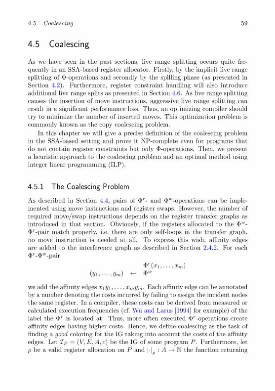
4.5 Coalescing 59
4.5 Coalescing
As we have seen in the past sections, live range splitting occurs quite fre-quently in an SSA-based register allocator. Firstly, by the implicit live rangesplitting of Φ-operations and secondly by the spilling phase (as presented inSection 4.2). Furthermore, register constraint handling will also introduceadditional live range splits as presented in Section 4.6. As live range splittingcauses the insertion of move instructions, aggressive live range splitting canresult in a significant performance loss. Thus, an optimizing compiler shouldtry to minimize the number of inserted moves. This optimization problem iscommonly known as the copy coalescing problem.
In this chapter we will give a precise definition of the coalescing problemin the SSA-based setting and prove it NP-complete even for programs thatdo not contain register constraints but only Φ-operations. Then, we presenta heuristic approach to the coalescing problem and an optimal method usinginteger linear programming (ILP).
4.5.1 The Coalescing Problem
As described in Section 4.4, pairs of Φr- and Φw-operations can be imple-mented using move instructions and register swaps. However, the number ofrequired move/swap instructions depends on the register transfer graphs asintroduced in that section. Obviously, if the registers allocated to the Φw-Φr-pair match properly, i.e. there are only self-loops in the transfer graph,no move instruction is needed at all. To express this wish, affinity edgesare added to the interference graph as described in Section 2.4.2. For eachΦr-Φw-pair
Φr(x1, . . . , xm)(y1, . . . , ym) ← Φw
we add the affinity edges x1y1, . . . , xmym. Each affinity edge can be annotatedby a number denoting the costs incurred by failing to assign the incident nodesthe same register. In a compiler, these costs can be derived from measured orcalculated execution frequencies (cf. Wu and Larus [1994] for example) of thelabel the Φr is located at. Thus, more often executed Φr-operations createaffinity edges having higher costs. Hence, we define coalescing as the task offinding a good coloring for the IG taking into account the costs of the affinityedges. Let IP = (V,E, A, c) be the IG of some program P . Furthermore, letρ be a valid register allocation on P and |·|ρ : A → N the function returning
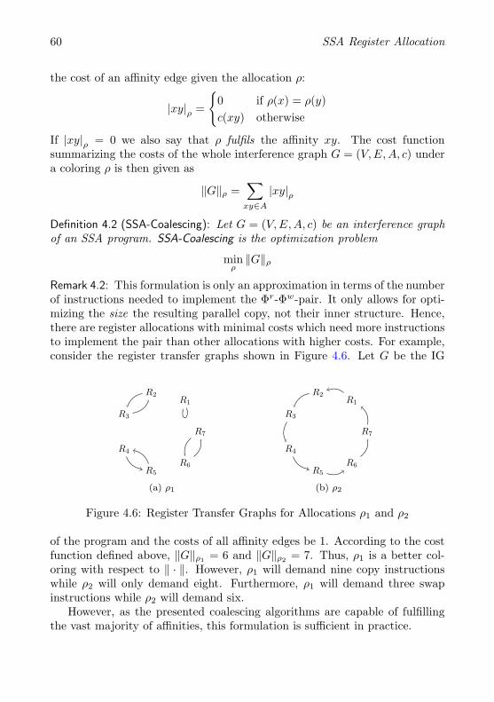
60 SSA Register Allocation
the cost of an affinity edge given the allocation ρ:
|xy|ρ =
{0 if ρ(x) = ρ(y)c(xy) otherwise
If |xy|ρ = 0 we also say that ρ fulfils the affinity xy. The cost functionsummarizing the costs of the whole interference graph G = (V,E, A, c) undera coloring ρ is then given as
‖G‖ρ =∑
xy∈A
|xy|ρ
Definition 4.2 (SSA-Coalescing): Let G = (V,E, A, c) be an interference graphof an SSA program. SSA-Coalescing is the optimization problem
minρ‖G‖ρ
Remark 4.2: This formulation is only an approximation in terms of the numberof instructions needed to implement the Φr-Φw-pair. It only allows for opti-mizing the size the resulting parallel copy, not their inner structure. Hence,there are register allocations with minimal costs which need more instructionsto implement the pair than other allocations with higher costs. For example,consider the register transfer graphs shown in Figure 4.6. Let G be the IG
R1
R2
R3
R4
R5
R6
R7
(a) ρ1
R1
R2
R3
R4
R5
R6
R7
(b) ρ2
Figure 4.6: Register Transfer Graphs for Allocations ρ1 and ρ2
of the program and the costs of all affinity edges be 1. According to the costfunction defined above, ‖G‖ρ1 = 6 and ‖G‖ρ2 = 7. Thus, ρ1 is a better col-oring with respect to ‖ · ‖. However, ρ1 will demand nine copy instructionswhile ρ2 will only demand eight. Furthermore, ρ1 will demand three swapinstructions while ρ2 will demand six.
However, as the presented coalescing algorithms are capable of fulfillingthe vast majority of affinities, this formulation is sufficient in practice.
4.5 Coalescing 61
4.5.1.1 The Complexity of SSA-Coalescing
Allowing arbitrary interference graphs G and especially arbitrary affinitiesbetween nodes of G, one can easily produce instances where coalescing directlycorresponds to a general graph coloring problem. This has also been notedby Appel and George [2001].
However, this does not provide the complexity of coalescing on graphsarising from SSA programs we are concerned with, since our graphs do notexhibit arbitrary structure. The interference part is chordal and the affinitypart is generated by live range splitting. For proving the NP-completenessof coalescing on this subset of graphs, we have to generate an SSA programfrom an instance of an NP-complete problem and show that coalescing onthe program’s interference graph induces a solution to the instance of theNP-complete problem.
The proof of the NP-completeness of SSA-Coalescing on SSA interferencegraphs is a classical reduction proof using graph coloring. First we select anarbitrary graph H and construct an SSA program from it. The Φ-operationsin that program are placed in a way that an optimal coalescing induces anoptimal coloring in H and vice versa. The technique is a variation of the oneused by Rastello et al. [2003].
Theorem 4.5: SSA-Coalescing is NP-complete concerning the number of Φ-op-erations in the program.
Proof. We reduce the NP-complete problem of finding a k-coloring of a graphH to SSA-Coalescing. We construct a SSA-form program from H in the fol-lowing way:
• There is one label ` containing a Φ-operation
(p1, . . . , pk)← Φ
v1 · · · v1
......
v|VH | · · · v|VH |
• For each node vi ∈ VH there is a variable vi, a label `i containing a
definition of vi and a control flow edge `i → `
• For each edge vivj ∈ EH we add two variables aij and aji and two labels`ij , `ji which contain a definition of aij and aji respectively.
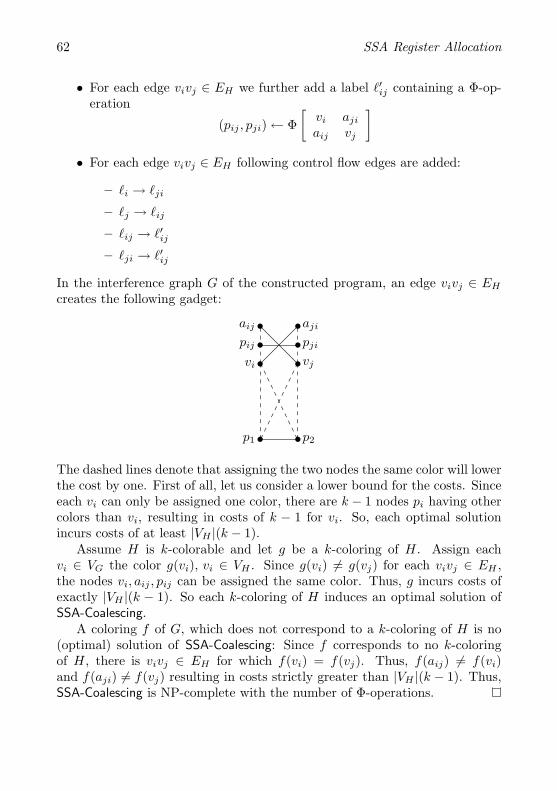
62 SSA Register Allocation
• For each edge vivj ∈ EH we further add a label `′ij containing a Φ-op-eration
(pij , pji)← Φ[
vi aji
aij vj
]• For each edge vivj ∈ EH following control flow edges are added:
– `i → `ji
– `j → `ij
– `ij → `′ij
– `ji → `′ij
In the interference graph G of the constructed program, an edge vivj ∈ EH
creates the following gadget:
vi
aij
vj
aji
pij pji
p1 p2
The dashed lines denote that assigning the two nodes the same color will lowerthe cost by one. First of all, let us consider a lower bound for the costs. Sinceeach vi can only be assigned one color, there are k − 1 nodes pi having othercolors than vi, resulting in costs of k − 1 for vi. So, each optimal solutionincurs costs of at least |VH |(k − 1).
Assume H is k-colorable and let g be a k-coloring of H. Assign eachvi ∈ VG the color g(vi), vi ∈ VH . Since g(vi) 6= g(vj) for each vivj ∈ EH ,the nodes vi, aij , pij can be assigned the same color. Thus, g incurs costs ofexactly |VH |(k − 1). So each k-coloring of H induces an optimal solution ofSSA-Coalescing.
A coloring f of G, which does not correspond to a k-coloring of H is no(optimal) solution of SSA-Coalescing: Since f corresponds to no k-coloringof H, there is vivj ∈ EH for which f(vi) = f(vj). Thus, f(aij) 6= f(vi)and f(aji) 6= f(vj) resulting in costs strictly greater than |VH |(k − 1). Thus,SSA-Coalescing is NP-complete with the number of Φ-operations.
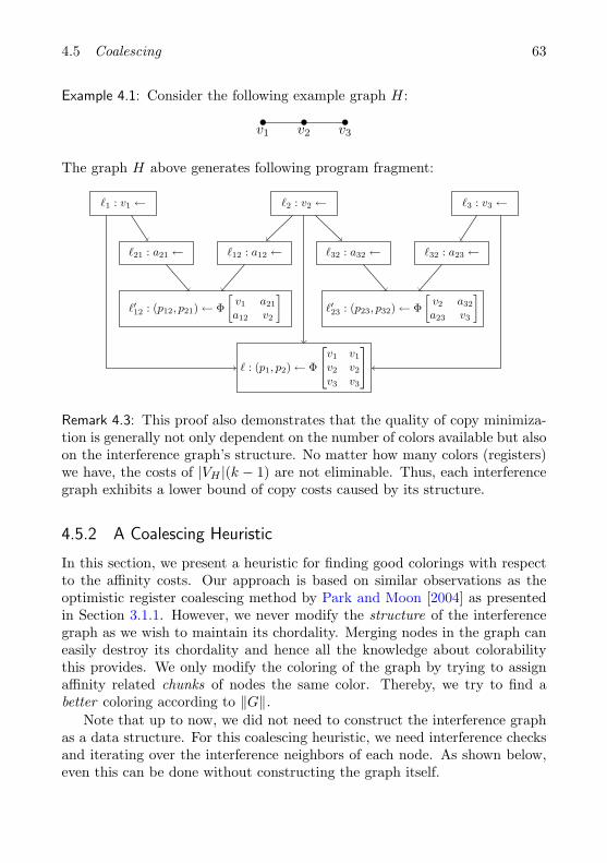
4.5 Coalescing 63
Example 4.1: Consider the following example graph H:
v1 v2 v3
The graph H above generates following program fragment:
`1 : v1 ← `2 : v2 ← `3 : v3 ←
`21 : a21 ← `12 : a12 ← `32 : a32 ← `32 : a23 ←
`′12 : (p12, p21)← Φ[
v1 a21
a12 v2
]`′23 : (p23, p32)← Φ
[v2 a32
a23 v3
]
` : (p1, p2)← Φ
v1 v1
v2 v2
v3 v3
Remark 4.3: This proof also demonstrates that the quality of copy minimiza-tion is generally not only dependent on the number of colors available but alsoon the interference graph’s structure. No matter how many colors (registers)we have, the costs of |VH |(k − 1) are not eliminable. Thus, each interferencegraph exhibits a lower bound of copy costs caused by its structure.
4.5.2 A Coalescing Heuristic
In this section, we present a heuristic for finding good colorings with respectto the affinity costs. Our approach is based on similar observations as theoptimistic register coalescing method by Park and Moon [2004] as presentedin Section 3.1.1. However, we never modify the structure of the interferencegraph as we wish to maintain its chordality. Merging nodes in the graph caneasily destroy its chordality and hence all the knowledge about colorabilitythis provides. We only modify the coloring of the graph by trying to assignaffinity related chunks of nodes the same color. Thereby, we try to find abetter coloring according to ‖G‖.
Note that up to now, we did not need to construct the interference graphas a data structure. For this coalescing heuristic, we need interference checksand iterating over the interference neighbors of each node. As shown below,even this can be done without constructing the graph itself.
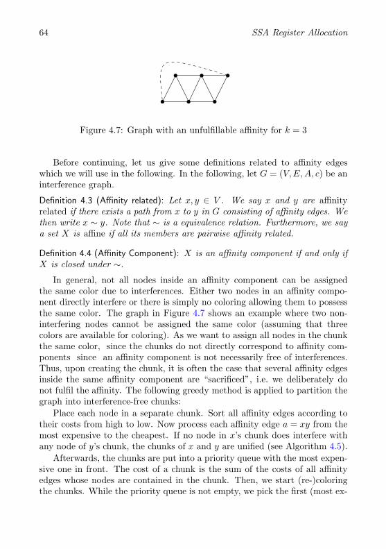
64 SSA Register Allocation
Figure 4.7: Graph with an unfulfillable affinity for k = 3
Before continuing, let us give some definitions related to affinity edgeswhich we will use in the following. In the following, let G = (V,E, A, c) be aninterference graph.
Definition 4.3 (Affinity related): Let x, y ∈ V . We say x and y are affinityrelated if there exists a path from x to y in G consisting of affinity edges. Wethen write x ∼ y. Note that ∼ is a equivalence relation. Furthermore, we saya set X is affine if all its members are pairwise affinity related.
Definition 4.4 (Affinity Component): X is an affinity component if and only ifX is closed under ∼.
In general, not all nodes inside an affinity component can be assignedthe same color due to interferences. Either two nodes in an affinity compo-nent directly interfere or there is simply no coloring allowing them to possessthe same color. The graph in Figure 4.7 shows an example where two non-interfering nodes cannot be assigned the same color (assuming that threecolors are available for coloring). As we want to assign all nodes in the chunkthe same color, since the chunks do not directly correspond to affinity com-ponents since an affinity component is not necessarily free of interferences.Thus, upon creating the chunk, it is often the case that several affinity edgesinside the same affinity component are “sacrificed”, i.e. we deliberately donot fulfil the affinity. The following greedy method is applied to partition thegraph into interference-free chunks:
Place each node in a separate chunk. Sort all affinity edges according totheir costs from high to low. Now process each affinity edge a = xy from themost expensive to the cheapest. If no node in x’s chunk does interfere withany node of y’s chunk, the chunks of x and y are unified (see Algorithm 4.5).
Afterwards, the chunks are put into a priority queue with the most expen-sive one in front. The cost of a chunk is the sum of the costs of all affinityedges whose nodes are contained in the chunk. Then, we start (re-)coloringthe chunks. While the priority queue is not empty, we pick the first (most ex-
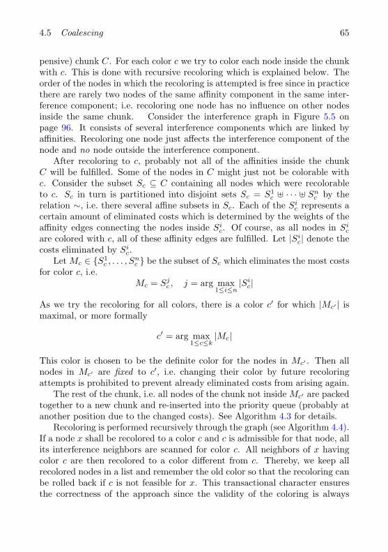
4.5 Coalescing 65
pensive) chunk C. For each color c we try to color each node inside the chunkwith c. This is done with recursive recoloring which is explained below. Theorder of the nodes in which the recoloring is attempted is free since in practicethere are rarely two nodes of the same affinity component in the same inter-ference component; i.e. recoloring one node has no influence on other nodesinside the same chunk. Consider the interference graph in Figure 5.5 onpage 96. It consists of several interference components which are linked byaffinities. Recoloring one node just affects the interference component of thenode and no node outside the interference component.
After recoloring to c, probably not all of the affinities inside the chunkC will be fulfilled. Some of the nodes in C might just not be colorable withc. Consider the subset Sc ⊆ C containing all nodes which were recolorableto c. Sc in turn is partitioned into disjoint sets Sc = S1
c ] · · · ] Snc by the
relation ∼, i.e. there several affine subsets in Sc. Each of the Sic represents a
certain amount of eliminated costs which is determined by the weights of theaffinity edges connecting the nodes inside Si
c. Of course, as all nodes in Sic
are colored with c, all of these affinity edges are fulfilled. Let |Sic| denote the
costs eliminated by Sic.
Let Mc ∈ {S1c , . . . , Sn
c } be the subset of Sc which eliminates the most costsfor color c, i.e.
Mc = Sjc , j = arg max
1≤i≤n|Si
c|
As we try the recoloring for all colors, there is a color c′ for which |Mc′ | ismaximal, or more formally
c′ = arg max1≤c≤k
|Mc|
This color is chosen to be the definite color for the nodes in Mc′ . Then allnodes in Mc′ are fixed to c′, i.e. changing their color by future recoloringattempts is prohibited to prevent already eliminated costs from arising again.
The rest of the chunk, i.e. all nodes of the chunk not inside Mc′ are packedtogether to a new chunk and re-inserted into the priority queue (probably atanother position due to the changed costs). See Algorithm 4.3 for details.
Recoloring is performed recursively through the graph (see Algorithm 4.4).If a node x shall be recolored to a color c and c is admissible for that node, allits interference neighbors are scanned for color c. All neighbors of x havingcolor c are then recolored to a color different from c. Thereby, we keep allrecolored nodes in a list and remember the old color so that the recoloring canbe rolled back if c is not feasible for x. This transactional character ensuresthe correctness of the approach since the validity of the coloring is always
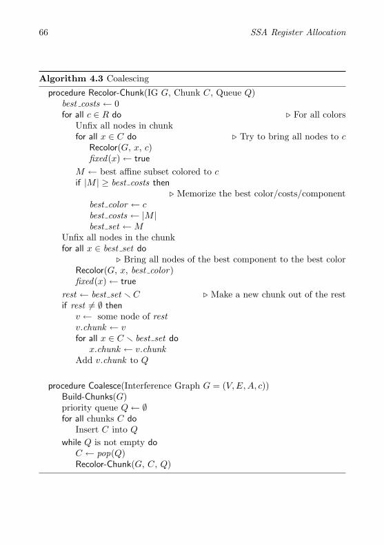
66 SSA Register Allocation
Algorithm 4.3 Coalescing
procedure Recolor-Chunk(IG G, Chunk C, Queue Q)best costs ← 0for all c ∈ R do . For all colors
Unfix all nodes in chunkfor all x ∈ C do . Try to bring all nodes to c
Recolor(G, x, c)fixed(x)← true
M ← best affine subset colored to cif |M | ≥ best costs then
. Memorize the best color/costs/componentbest color ← cbest costs ← |M |best set ←M
Unfix all nodes in the chunkfor all x ∈ best set do
. Bring all nodes of the best component to the best colorRecolor(G, x, best color)fixed(x)← true
rest ← best set r C . Make a new chunk out of the restif rest 6= ∅ then
v ← some node of restv.chunk ← vfor all x ∈ C r best set do
x.chunk ← v.chunkAdd v.chunk to Q
procedure Coalesce(Interference Graph G = (V,E, A, c))Build-Chunks(G)priority queue Q← ∅for all chunks C do
Insert C into Q
while Q is not empty doC ← pop(Q)Recolor-Chunk(G, C, Q)
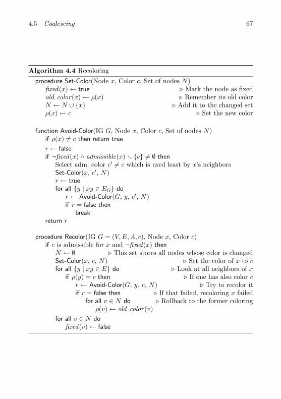
4.5 Coalescing 67
Algorithm 4.4 Recoloring
procedure Set-Color(Node x, Color c, Set of nodes N)fixed(x)← true . Mark the node as fixedold color(x)← ρ(x) . Remember its old colorN ← N ∪ {x} . Add it to the changed setρ(x)← c . Set the new color
function Avoid-Color(IG G, Node x, Color c, Set of nodes N)if ρ(x) 6= c then return true
r ← falseif ¬fixed(x) ∧ admissible(x) r {c} 6= ∅ then
Select adm. color c′ 6= c which is used least by x’s neighborsSet-Color(x, c′, N)r ← truefor all {y | xy ∈ EG} do
r ← Avoid-Color(G, y, c′, N)if r = false then
breakreturn r
procedure Recolor(IG G = (V,E, A, c), Node x, Color c)if c is admissible for x and ¬fixed(x) then
N ← ∅ . This set stores all nodes whose color is changedSet-Color(x, c, N) . Set the color of x to cfor all {y | xy ∈ E} do . Look at all neighbors of x
if ρ(y) = c then . If one has also color cr ← Avoid-Color(G, y, c, N) . Try to recolor itif r = false then . If that failed, recoloring x failed
for all v ∈ N do . Rollback to the former coloringρ(v)← old color(v)
for all v ∈ N dofixed(v)← false
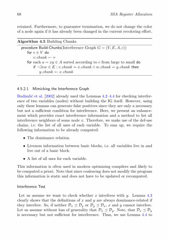
68 SSA Register Allocation
retained. Furthermore, to guarantee termination, we do not change the colorof a node again if it has already been changed in the current recoloring effort.
Algorithm 4.5 Building Chunks
procedure Build-Chunks(Interference Graph G = (V,E, A, c))for v ∈ V do
v.chunk ← vfor each a = xy ∈ A sorted according to c from large to small do
if ¬∃vw ∈ E : v.chunk = x.chunk ∧ w.chunk = y.chunk theny.chunk ← x.chunk
4.5.2.1 Mimicking the Interference Graph
Budimlic et al. [2002] already used the Lemmas 4.2–4.4 for checking interfer-ence of two variables (nodes) without building the IG itself. However, usingonly these lemmas can generate false positives since they are only a necessarybut not a sufficient condition for interference. Here, we present an enhance-ment which provides exact interference information and a method to list allinterference neighbors of some node x. Therefore, we make use of the def-usechains, i.e. the list of all uses of each variable. To sum up, we require thefollowing information to be already computed:
• The dominance relation.
• Liveness information between basic blocks, i.e. all variables live in andlive out of a basic block.
• A list of all uses for each variable.
This information is often used in modern optimizing compilers and likely tobe computed a priori. Note that since coalescing does not modify the programthis information is static and does not have to be updated or recomputed.
Interference Test
Let us assume we want to check whether x interferes with y. Lemma 4.3clearly shows that the definitions of x and y are always dominance-related ifthey interfere. So, if neither Dx � Dy or Dy � Dx, x and y cannot interfere.Let us assume without loss of generality that Dx � Dy. Note, that Dx � Dy
is necessary but not sufficient for interference. Thus, we use Lemma 4.4 to
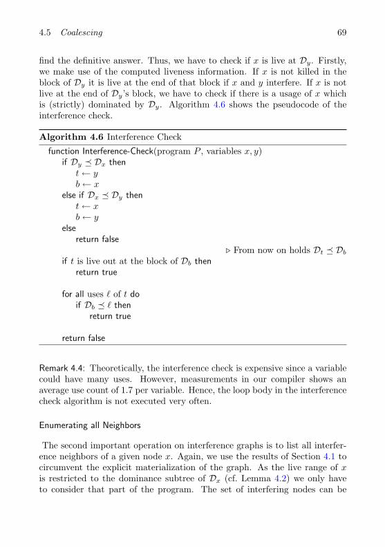
4.5 Coalescing 69
find the definitive answer. Thus, we have to check if x is live at Dy. Firstly,we make use of the computed liveness information. If x is not killed in theblock of Dy it is live at the end of that block if x and y interfere. If x is notlive at the end of Dy’s block, we have to check if there is a usage of x whichis (strictly) dominated by Dy. Algorithm 4.6 shows the pseudocode of theinterference check.
Algorithm 4.6 Interference Check
function Interference-Check(program P , variables x, y)if Dy � Dx then
t← yb← x
else if Dx � Dy thent← xb← y
elsereturn false
. From now on holds Dt � Db
if t is live out at the block of Db thenreturn true
for all uses ` of t doif Db � ` then
return true
return false
Remark 4.4: Theoretically, the interference check is expensive since a variablecould have many uses. However, measurements in our compiler shows anaverage use count of 1.7 per variable. Hence, the loop body in the interferencecheck algorithm is not executed very often.
Enumerating all Neighbors
The second important operation on interference graphs is to list all interfer-ence neighbors of a given node x. Again, we use the results of Section 4.1 tocircumvent the explicit materialization of the graph. As the live range of xis restricted to the dominance subtree of Dx (cf. Lemma 4.2) we only haveto consider that part of the program. The set of interfering nodes can be
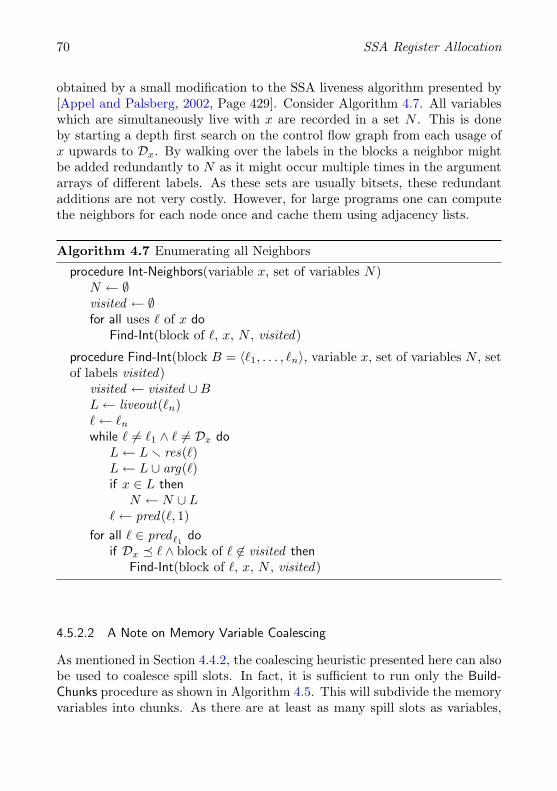
70 SSA Register Allocation
obtained by a small modification to the SSA liveness algorithm presented by[Appel and Palsberg, 2002, Page 429]. Consider Algorithm 4.7. All variableswhich are simultaneously live with x are recorded in a set N . This is doneby starting a depth first search on the control flow graph from each usage ofx upwards to Dx. By walking over the labels in the blocks a neighbor mightbe added redundantly to N as it might occur multiple times in the argumentarrays of different labels. As these sets are usually bitsets, these redundantadditions are not very costly. However, for large programs one can computethe neighbors for each node once and cache them using adjacency lists.
Algorithm 4.7 Enumerating all Neighbors
procedure Int-Neighbors(variable x, set of variables N)N ← ∅visited ← ∅for all uses ` of x do
Find-Int(block of `, x, N , visited)
procedure Find-Int(block B = 〈`1, . . . , `n〉, variable x, set of variables N , setof labels visited)
visited ← visited ∪BL← liveout(`n)`← `n
while ` 6= `1 ∧ ` 6= Dx doL← L r res(`)L← L ∪ arg(`)if x ∈ L then
N ← N ∪ L`← pred(`, 1)
for all ` ∈ pred `1 doif Dx � ` ∧ block of ` 6∈ visited then
Find-Int(block of `, x, N , visited)
4.5.2.2 A Note on Memory Variable Coalescing
As mentioned in Section 4.4.2, the coalescing heuristic presented here can alsobe used to coalesce spill slots. In fact, it is sufficient to run only the Build-Chunks procedure as shown in Algorithm 4.5. This will subdivide the memoryvariables into chunks. As there are at least as many spill slots as variables,
4.5 Coalescing 71
each resulting chunk can be assigned a different spill slot. Hence, recursiverecoloring is not necessary for memory variable coalescing.
4.5.3 Optimal Coalescing by ILP
In this section we describe a method yielding optimal solutions for SSA-Coalescing using integer linear programming (ILP). For readers not famil-iar with basic ILP terminology, we refer to Appendix B. Firstly, we give astandard problem formulation for SSA-Coalescing. Then, we present furtherrefinements of the formulation to prune the search space for the ILP solver.This work has been contributed by Grund [2005] in his diploma thesis and ispresented in Grund and Hack [2007].
4.5.3.1 Formalization
Let IP = (V,E, A, c) be the interference graph of some program P . Sinceevery solution of SSA-Coalescing is also a valid coloring, we start by modelinga common graph coloring problem. For each vi ∈ V and each possible color cthe binary variables xic indicate the color of node vi: if xic = 1 the variablexi has color c. The following constraint enforces that each node has exactlyone color:
∀vi ∈ V :∑
c
xic = 1
Furthermore, incident nodes must have different colors. Normally, constraintslike xic +xjc ≤ 1 are used for each edge xixj in the graph. For chordal graphsthe number of these inequalities can be drastically lowered using a minimumclique cover:
Definition 4.5 (Minimum Clique Cover, MCC): A minimum clique cover of agraph G is a minimal set of cliques {C1, . . . , Cm} such that VG = VC1 ∪ · · · ∪VCm .
For general graphs finding a MCC is NP-complete. However, for chordalgraphs a MCC can be computed in O(|V |2), see Gavril [1972] for example.Given a MCC {C1, . . . , Cm}, the edges in the graph can be modeled by cliqueinequations expressing that no two nodes in the same clique can have thesame color. Thus, we add for each Cj in the MCC and each color c:∑
vi∈Cj
xic ≤ 1
72 SSA Register Allocation
Register constraints (as discussed in Section 4.6) can be integrated in themodel by either setting the forbidden xic to 0, or by omitting the correspond-ing variables and adjusting the respective constraints accordingly.
So far, the model results in a valid coloring of G. Now we define the costfunction and add additional variables and constraints to model the affinities.For each edge vivj ∈ A the binary variable yij shall indicate, whether theincident nodes have the same color (yij = 0), or different colors (yij = 1).To model the positive costs c(vivj) arising from assigning vi and vj differentcolors, the cost function to be minimized is given by∑
vivj∈A
c(vivj) · yij
To relate the y to the x variables, we add a constraint per color and affinityedge in A. Since the yij are automatically forced towards 0 due to minimiza-tion, we only must enforce yij = 1, if vi and vj have different colors:
yij ≥ xic − xjc
yij ≥ xjc − xic
Our measurements (see Grund and Hack [2007]) showed that the ILPsolving process takes very long if the solver is provided solely the equationspresented above. Therefore, we present two improvements to the ILP for-mulation which significantly decrease the solution time of the ILP. The firstimprovement aims at reducing the size of the problem by modelling only “rel-evant” nodes of the IG in the ILP. This is achieved by exploiting a simplegraph theoretical observation. The second improvement increases the size ofthe problem by adding additional inequalities. However, these new inequal-ities are so called cuts, i.e. they do not rule out any feasible solutions butshrink the search space. One could say, they provide the solver with moreknowledge about the problem’s structure to enable it to detect and discardinvalid solutions earlier.
4.5.3.2 Reducing the Problem Size
To reduce the number of variables and constraints, we use the same observa-tion as the coloring heuristic presented in Section 3.1: if a node has less thank neighbors, it definitely can be colored. Hence, before setting up the ILP, weremove successively all nodes from G, which have less than k neighbors anddo exhibit neither affinities nor register constraints. The remaining graph G′
then represents the “core” of the problem. The coloring for G′ found by theILP solver can then be completed by adding the removed nodes again.
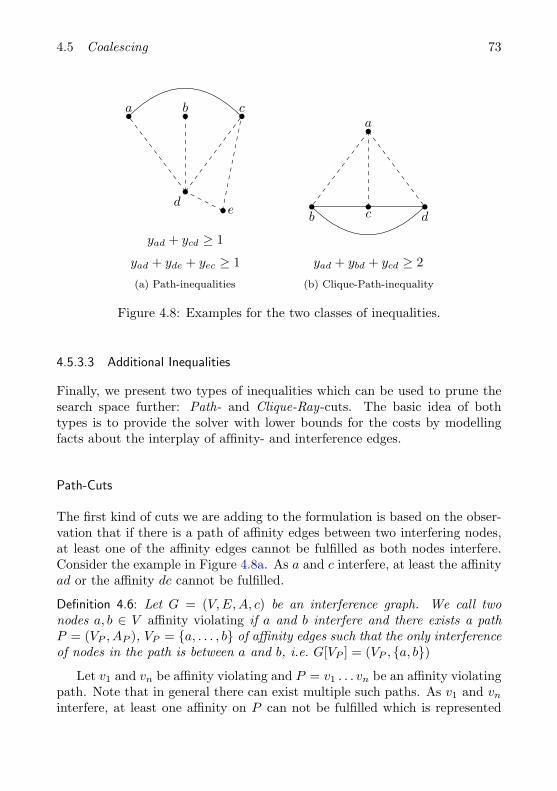
4.5 Coalescing 73
ed
a b c
yad + ycd ≥ 1
yad + yde + yec ≥ 1
(a) Path-inequalities
b c d
a
yad + ybd + ycd ≥ 2
(b) Clique-Path-inequality
Figure 4.8: Examples for the two classes of inequalities.
4.5.3.3 Additional Inequalities
Finally, we present two types of inequalities which can be used to prune thesearch space further: Path- and Clique-Ray-cuts. The basic idea of bothtypes is to provide the solver with lower bounds for the costs by modellingfacts about the interplay of affinity- and interference edges.
Path-Cuts
The first kind of cuts we are adding to the formulation is based on the obser-vation that if there is a path of affinity edges between two interfering nodes,at least one of the affinity edges cannot be fulfilled as both nodes interfere.Consider the example in Figure 4.8a. As a and c interfere, at least the affinityad or the affinity dc cannot be fulfilled.
Definition 4.6: Let G = (V,E, A, c) be an interference graph. We call twonodes a, b ∈ V affinity violating if a and b interfere and there exists a pathP = (VP , AP ), VP = {a, . . . , b} of affinity edges such that the only interferenceof nodes in the path is between a and b, i.e. G[VP ] = (VP , {a, b})
Let v1 and vn be affinity violating and P = v1 . . . vn be an affinity violatingpath. Note that in general there can exist multiple such paths. As v1 and vn
interfere, at least one affinity on P can not be fulfilled which is represented
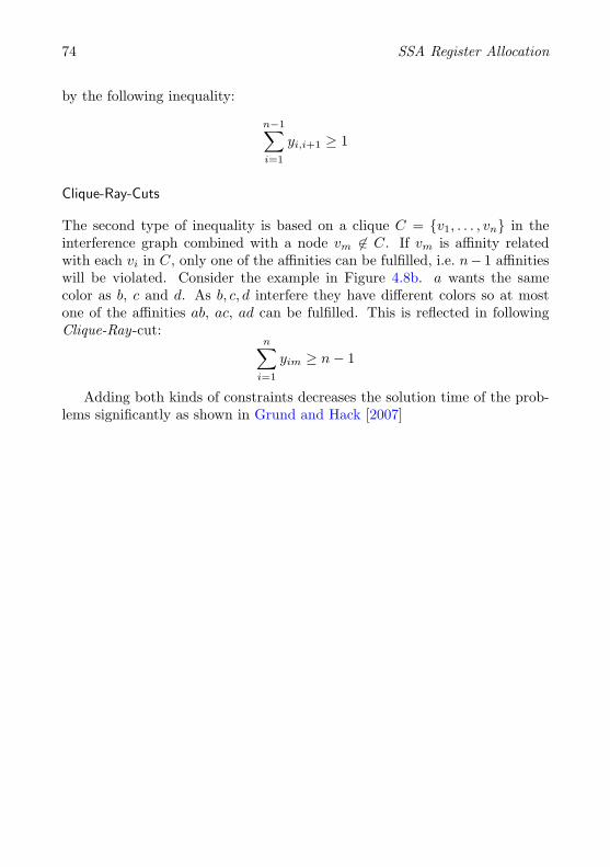
74 SSA Register Allocation
by the following inequality:
n−1∑i=1
yi,i+1 ≥ 1
Clique-Ray-Cuts
The second type of inequality is based on a clique C = {v1, . . . , vn} in theinterference graph combined with a node vm 6∈ C. If vm is affinity relatedwith each vi in C, only one of the affinities can be fulfilled, i.e. n− 1 affinitieswill be violated. Consider the example in Figure 4.8b. a wants the samecolor as b, c and d. As b, c, d interfere they have different colors so at mostone of the affinities ab, ac, ad can be fulfilled. This is reflected in followingClique-Ray-cut:
n∑i=1
yim ≥ n− 1
Adding both kinds of constraints decreases the solution time of the prob-lems significantly as shown in Grund and Hack [2007]
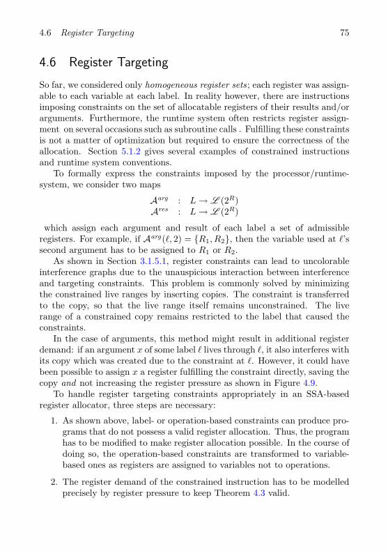
4.6 Register Targeting 75
4.6 Register Targeting
So far, we considered only homogeneous register sets; each register was assign-able to each variable at each label. In reality however, there are instructionsimposing constraints on the set of allocatable registers of their results and/orarguments. Furthermore, the runtime system often restricts register assign-ment on several occasions such as subroutine calls . Fulfilling these constraintsis not a matter of optimization but required to ensure the correctness of theallocation. Section 5.1.2 gives several examples of constrained instructionsand runtime system conventions.
To formally express the constraints imposed by the processor/runtime-system, we consider two maps
Aarg : L→ L (2R)Ares : L→ L (2R)
which assign each argument and result of each label a set of admissibleregisters. For example, if Aarg(`, 2) = {R1, R2}, then the variable used at `’ssecond argument has to be assigned to R1 or R2.
As shown in Section 3.1.5.1, register constraints can lead to uncolorableinterference graphs due to the unauspicious interaction between interferenceand targeting constraints. This problem is commonly solved by minimizingthe constrained live ranges by inserting copies. The constraint is transferredto the copy, so that the live range itself remains unconstrained. The liverange of a constrained copy remains restricted to the label that caused theconstraints.
In the case of arguments, this method might result in additional registerdemand: if an argument x of some label ` lives through `, it also interferes withits copy which was created due to the constraint at `. However, it could havebeen possible to assign x a register fulfilling the constraint directly, saving thecopy and not increasing the register pressure as shown in Figure 4.9.
To handle register targeting constraints appropriately in an SSA-basedregister allocator, three steps are necessary:
1. As shown above, label- or operation-based constraints can produce pro-grams that do not possess a valid register allocation. Thus, the programhas to be modified to make register allocation possible. In the course ofdoing so, the operation-based constraints are transformed to variable-based ones as registers are assigned to variables not to operations.
2. The register demand of the constrained instruction has to be modelledprecisely by register pressure to keep Theorem 4.3 valid.
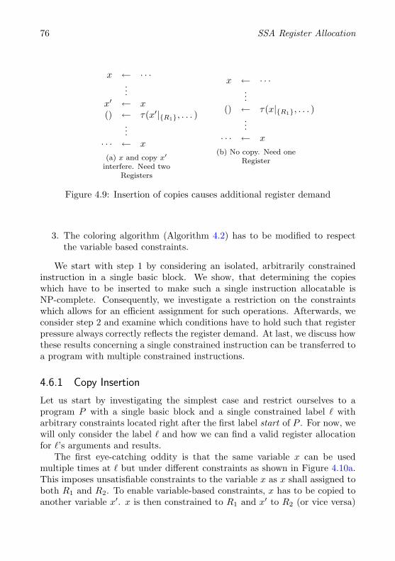
76 SSA Register Allocation
x ← · · ·...
x′ ← x() ← τ(x′|{R1}, . . . )
...· · · ← x
(a) x and copy x′
interfere. Need twoRegisters
x ← · · ·...
() ← τ(x|{R1}, . . . )...
· · · ← x
(b) No copy. Need oneRegister
Figure 4.9: Insertion of copies causes additional register demand
3. The coloring algorithm (Algorithm 4.2) has to be modified to respectthe variable based constraints.
We start with step 1 by considering an isolated, arbitrarily constrainedinstruction in a single basic block. We show, that determining the copieswhich have to be inserted to make such a single instruction allocatable isNP-complete. Consequently, we investigate a restriction on the constraintswhich allows for an efficient assignment for such operations. Afterwards, weconsider step 2 and examine which conditions have to hold such that registerpressure always correctly reflects the register demand. At last, we discuss howthese results concerning a single constrained instruction can be transferred toa program with multiple constrained instructions.
4.6.1 Copy Insertion
Let us start by investigating the simplest case and restrict ourselves to aprogram P with a single basic block and a single constrained label ` witharbitrary constraints located right after the first label start of P . For now, wewill only consider the label ` and how we can find a valid register allocationfor `’s arguments and results.
The first eye-catching oddity is that the same variable x can be usedmultiple times at ` but under different constraints as shown in Figure 4.10a.This imposes unsatisfiable constraints to the variable x as x shall assigned toboth R1 and R2. To enable variable-based constraints, x has to be copied toanother variable x′. x is then constrained to R1 and x′ to R2 (or vice versa)
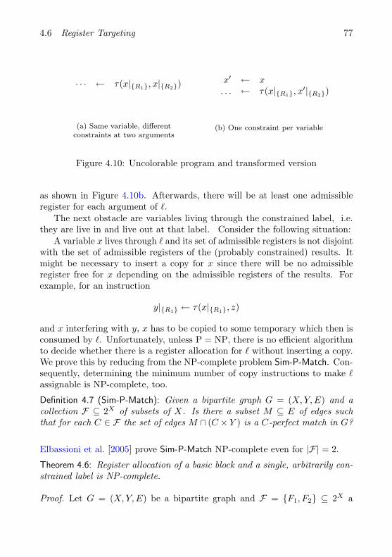
4.6 Register Targeting 77
· · · ← τ(x|{R1}, x|{R2})
(a) Same variable, differentconstraints at two arguments
x′ ← x. . . ← τ(x|{R1}, x
′|{R2})
(b) One constraint per variable
Figure 4.10: Uncolorable program and transformed version
as shown in Figure 4.10b. Afterwards, there will be at least one admissibleregister for each argument of `.
The next obstacle are variables living through the constrained label, i.e.they are live in and live out at that label. Consider the following situation:
A variable x lives through ` and its set of admissible registers is not disjointwith the set of admissible registers of the (probably constrained) results. Itmight be necessary to insert a copy for x since there will be no admissibleregister free for x depending on the admissible registers of the results. Forexample, for an instruction
y|{R1} ← τ(x|{R1}, z)
and x interfering with y, x has to be copied to some temporary which then isconsumed by `. Unfortunately, unless P = NP, there is no efficient algorithmto decide whether there is a register allocation for ` without inserting a copy.We prove this by reducing from the NP-complete problem Sim-P-Match. Con-sequently, determining the minimum number of copy instructions to make `assignable is NP-complete, too.
Definition 4.7 (Sim-P-Match): Given a bipartite graph G = (X, Y,E) and acollection F ⊆ 2X of subsets of X. Is there a subset M ⊆ E of edges suchthat for each C ∈ F the set of edges M ∩ (C × Y ) is a C-perfect match in G?
Elbassioni et al. [2005] prove Sim-P-Match NP-complete even for |F| = 2.
Theorem 4.6: Register allocation of a basic block and a single, arbitrarily con-strained label is NP-complete.
Proof. Let G = (X, Y,E) be a bipartite graph and F = {F1, F2} ⊆ 2X a
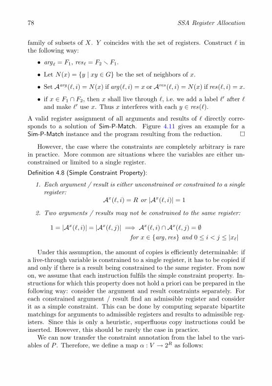
78 SSA Register Allocation
family of subsets of X. Y coincides with the set of registers. Construct ` inthe following way:
• arg` = F1, res` = F2 r F1.
• Let N(x) = {y | xy ∈ G} be the set of neighbors of x.
• Set Aarg(`, i) = N(x) if arg(`, i) = x or Ares(`, i) = N(x) if res(`, i) = x.
• if x ∈ F1 ∩ F2, then x shall live through `, i.e. we add a label `′ after `and make `′ use x. Thus x interferes with each y ∈ res(`).
A valid register assignment of all arguments and results of ` directly corre-sponds to a solution of Sim-P-Match. Figure 4.11 gives an example for aSim-P-Match instance and the program resulting from the reduction.
However, the case where the constraints are completely arbitrary is rarein practice. More common are situations where the variables are either un-constrained or limited to a single register.
Definition 4.8 (Simple Constraint Property):
1. Each argument / result is either unconstrained or constrained to a singleregister:
Ax(`, i) = R or |Ax(`, i)| = 1
2. Two arguments / results may not be constrained to the same register:
1 = |Ax(`, i)| = |Ax(`, j)| =⇒ Ax(`, i) ∩ Ax(`, j) = ∅for x ∈ {arg , res} and 0 ≤ i < j ≤ |x`|
Under this assumption, the amount of copies is efficiently determinable: ifa live-through variable is constrained to a single register, it has to be copied ifand only if there is a result being constrained to the same register. From nowon, we assume that each instruction fulfils the simple constraint property. In-structions for which this property does not hold a priori can be prepared in thefollowing way: consider the argument and result constraints separately. Foreach constrained argument / result find an admissible register and considerit as a simple constraint. This can be done by computing separate bipartitematchings for arguments to admissible registers and results to admissible reg-isters. Since this is only a heuristic, superfluous copy instructions could beinserted. However, this should be rarely the case in practice.
We can now transfer the constraint annotation from the label to the vari-ables of P . Therefore, we define a map α : V → 2R as follows:
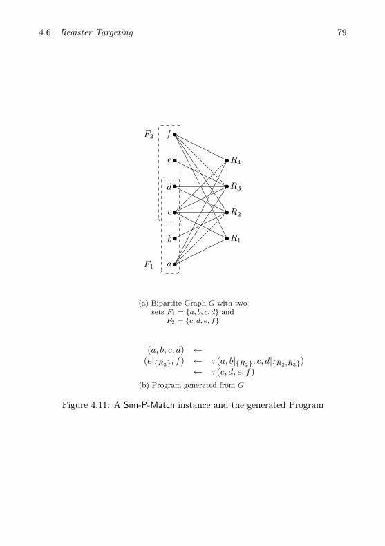
4.6 Register Targeting 79
a
b
c
d
e
f
R1
R2
R3
R4
F1
F2
(a) Bipartite Graph G with twosets F1 = {a, b, c, d} and
F2 = {c, d, e, f}
(a, b, c, d) ←(e|{R3}, f) ← τ(a, b|{R2}, c, d|{R2,R3})
← τ(c, d, e, f)(b) Program generated from G
Figure 4.11: A Sim-P-Match instance and the generated Program
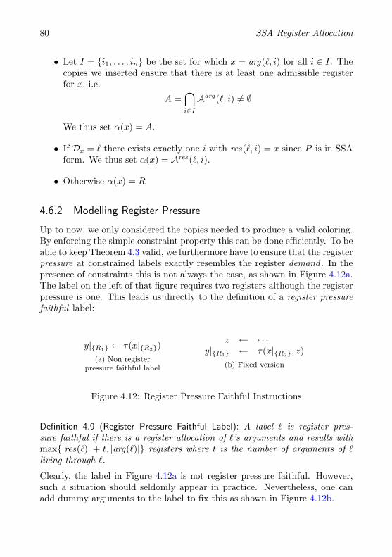
80 SSA Register Allocation
• Let I = {i1, . . . , in} be the set for which x = arg(`, i) for all i ∈ I. Thecopies we inserted ensure that there is at least one admissible registerfor x, i.e.
A =⋂i∈I
Aarg(`, i) 6= ∅
We thus set α(x) = A.
• If Dx = ` there exists exactly one i with res(`, i) = x since P is in SSAform. We thus set α(x) = Ares(`, i).
• Otherwise α(x) = R
4.6.2 Modelling Register Pressure
Up to now, we only considered the copies needed to produce a valid coloring.By enforcing the simple constraint property this can be done efficiently. To beable to keep Theorem 4.3 valid, we furthermore have to ensure that the registerpressure at constrained labels exactly resembles the register demand . In thepresence of constraints this is not always the case, as shown in Figure 4.12a.The label on the left of that figure requires two registers although the registerpressure is one. This leads us directly to the definition of a register pressurefaithful label:
y|{R1} ← τ(x|{R2})(a) Non register
pressure faithful label
z ← · · ·y|{R1} ← τ(x|{R2}, z)
(b) Fixed version
Figure 4.12: Register Pressure Faithful Instructions
Definition 4.9 (Register Pressure Faithful Label): A label ` is register pres-sure faithful if there is a register allocation of `’s arguments and results withmax{|res(`)| + t, |arg(`)|} registers where t is the number of arguments of `living through `.
Clearly, the label in Figure 4.12a is not register pressure faithful. However,such a situation should seldomly appear in practice. Nevertheless, one canadd dummy arguments to the label to fix this as shown in Figure 4.12b.
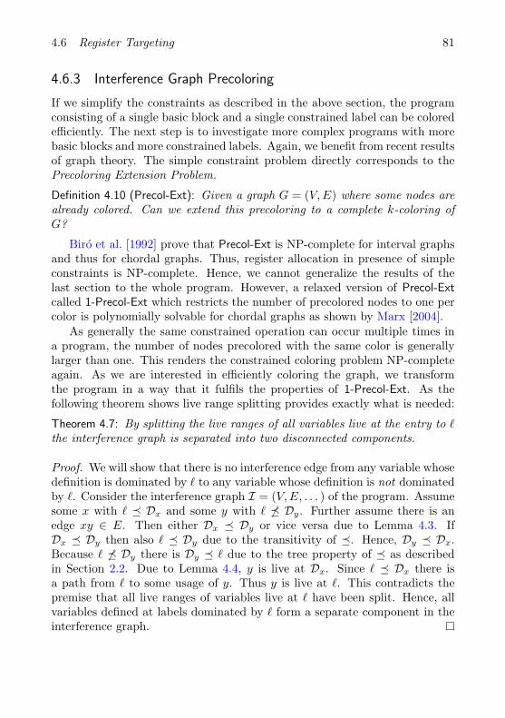
4.6 Register Targeting 81
4.6.3 Interference Graph Precoloring
If we simplify the constraints as described in the above section, the programconsisting of a single basic block and a single constrained label can be coloredefficiently. The next step is to investigate more complex programs with morebasic blocks and more constrained labels. Again, we benefit from recent resultsof graph theory. The simple constraint problem directly corresponds to thePrecoloring Extension Problem.
Definition 4.10 (Precol-Ext): Given a graph G = (V,E) where some nodes arealready colored. Can we extend this precoloring to a complete k-coloring ofG?
Biro et al. [1992] prove that Precol-Ext is NP-complete for interval graphsand thus for chordal graphs. Thus, register allocation in presence of simpleconstraints is NP-complete. Hence, we cannot generalize the results of thelast section to the whole program. However, a relaxed version of Precol-Extcalled 1-Precol-Ext which restricts the number of precolored nodes to one percolor is polynomially solvable for chordal graphs as shown by Marx [2004].
As generally the same constrained operation can occur multiple times ina program, the number of nodes precolored with the same color is generallylarger than one. This renders the constrained coloring problem NP-completeagain. As we are interested in efficiently coloring the graph, we transformthe program in a way that it fulfils the properties of 1-Precol-Ext. As thefollowing theorem shows live range splitting provides exactly what is needed:
Theorem 4.7: By splitting the live ranges of all variables live at the entry to `the interference graph is separated into two disconnected components.
Proof. We will show that there is no interference edge from any variable whosedefinition is dominated by ` to any variable whose definition is not dominatedby `. Consider the interference graph I = (V,E, . . . ) of the program. Assumesome x with ` � Dx and some y with ` 6� Dy. Further assume there is anedge xy ∈ E. Then either Dx � Dy or vice versa due to Lemma 4.3. IfDx � Dy then also ` � Dy due to the transitivity of �. Hence, Dy � Dx.Because ` 6� Dy there is Dy � ` due to the tree property of � as describedin Section 2.2. Due to Lemma 4.4, y is live at Dx. Since ` � Dx there isa path from ` to some usage of y. Thus y is live at `. This contradicts thepremise that all live ranges of variables live at ` have been split. Hence, allvariables defined at labels dominated by ` form a separate component in theinterference graph.
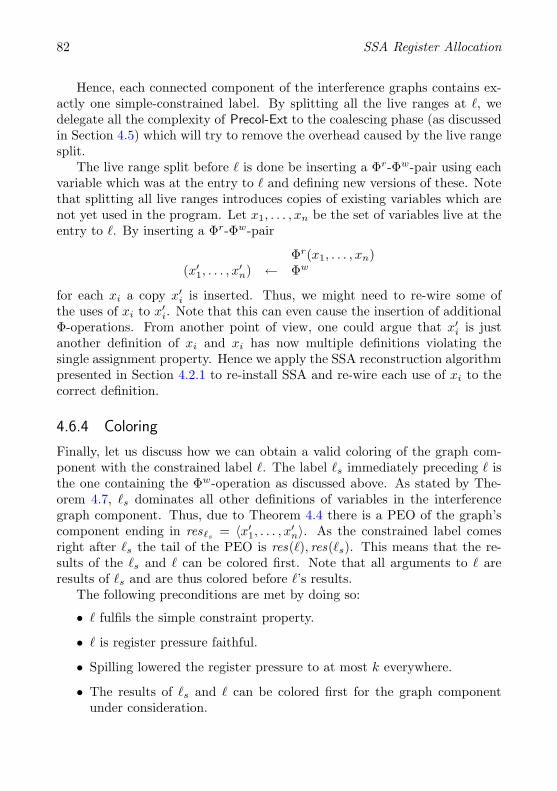
82 SSA Register Allocation
Hence, each connected component of the interference graphs contains ex-actly one simple-constrained label. By splitting all the live ranges at `, wedelegate all the complexity of Precol-Ext to the coalescing phase (as discussedin Section 4.5) which will try to remove the overhead caused by the live rangesplit.
The live range split before ` is done be inserting a Φr-Φw-pair using eachvariable which was at the entry to ` and defining new versions of these. Notethat splitting all live ranges introduces copies of existing variables which arenot yet used in the program. Let x1, . . . , xn be the set of variables live at theentry to `. By inserting a Φr-Φw-pair
Φr(x1, . . . , xn)(x′1, . . . , x
′n) ← Φw
for each xi a copy x′i is inserted. Thus, we might need to re-wire some ofthe uses of xi to x′i. Note that this can even cause the insertion of additionalΦ-operations. From another point of view, one could argue that x′i is justanother definition of xi and xi has now multiple definitions violating thesingle assignment property. Hence we apply the SSA reconstruction algorithmpresented in Section 4.2.1 to re-install SSA and re-wire each use of xi to thecorrect definition.
4.6.4 Coloring
Finally, let us discuss how we can obtain a valid coloring of the graph com-ponent with the constrained label `. The label `s immediately preceding ` isthe one containing the Φw-operation as discussed above. As stated by The-orem 4.7, `s dominates all other definitions of variables in the interferencegraph component. Thus, due to Theorem 4.4 there is a PEO of the graph’scomponent ending in res`s = 〈x′1, . . . , x′n〉. As the constrained label comesright after `s the tail of the PEO is res(`), res(`s). This means that the re-sults of the `s and ` can be colored first. Note that all arguments to ` areresults of `s and are thus colored before `’s results.
The following preconditions are met by doing so:
• ` fulfils the simple constraint property.
• ` is register pressure faithful.
• Spilling lowered the register pressure to at most k everywhere.
• The results of `s and ` can be colored first for the graph componentunder consideration.
4.6 Register Targeting 83
We thus assign all constrained variables their color. Note that the simple con-straint property restricts a constrained variable to a single register. Furthernote that the register pressure truth guarantees that there is a valid registerallocation of `’s arguments and results with r = max{|res(`)| + t, |arg(`)|}registers. As the register pressure before ` is at least |arg(`)| and after ` atleast t+ |res(`)|, there can only be k−r variables live through ` without beingused by `. As ` needs at most r registers there will be enough registers forall variables living by `. So our only task is to find a register allocation of `needing no more than r registers.
Algorithm 4.8 computes the initial coloring at a constrained label. Firstly,all constrained variables at ` are colored with their designated color. After-wards, all arguments dying at ` are colored. Thereby, colors used by theconstrained results are re-used if possible (not already in use by an argu-ment). The same applies to the remaining unconstrained results. At last, allarguments live through ` (set T ) have to be colored with colors different fromthose already used, since they interfere with both the dying variables (set A)and the variables defined (set D).
To complete the coloring for the labels `s and `, all variables defined bythe Φw at `s which are not used at ` have to be colored with colors not usedby any argument or result of `. The rest of the component can be coloredwith Algorithm 4.2 starting with the label after `.
4.6.5 An Example
To demonstrate the process of register targeting in an SSA-based registerallocator, we consider a call instruction on the x86 platform. Processors ofthe x86 family provide seven general purpose registers named eax, ebx, ecx,edx, esi, edi, ebp. The GNU C compiler provides a fast call extension bywhich the first two (integer) parameters to a function can be passed in theregisters ecx and edx. All other parameters are passed on the stack. Theregisters eax, ecx, edx may be overwritten by the callee, i.e. they are caller-save. The other registers have to be saved by the callee if necessary, i.e. theyare callee-save.
For functions returning an integer (which we assume for this example), theresult of the function call is passed in eax. As the caller has to assume thatthe contents of the caller-save registers are destroyed upon returning from thecall, they can be treated as if they were additional call results. Hence, weinsert two dummy variables d1 and d2 to model the destruction of edx andecx after the call. Let us furthermore assume that the call is indirect, i.e.the called address is passed in a register which is not constrained. Consider
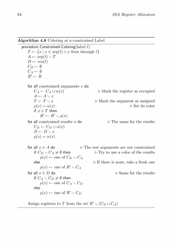
84 SSA Register Allocation
Algorithm 4.8 Coloring at a constrained Label
procedure Constrained-Coloring(label `)T ← {x | x ∈ arg(`) ∧ x lives through `}A← arg(`) r TD ← res(`)CR ← ∅CA ← ∅R′ ← R
for all constrained arguments x doCA ← CA ∪ α(x) . Mark the register as occupiedA← A r xT ← T r x . Mark the argument as assignedρ(x) = α(x) . Set its colorif x ∈ T then
R′ ← R′ r ρ(x)for all constrained results x do . The same for the results
CD ← CD ∪ α(x)D ← D r xρ(x) = α(x)
for all x ∈ A do . The rest arguments are not constrainedif CD r CA 6= ∅ then . Try to use a color of the results
ρ(x)← one of CD r CA
else . If there is none, take a fresh oneρ(x)← one of R′ r CA
for all x ∈ D do . Same for the resultsif CA r CD 6= ∅ then
ρ(x)← one of CA r CD
elseρ(x)← one of R′ r CD
Assign registers to T from the set R′ r (CD ∪ CA)
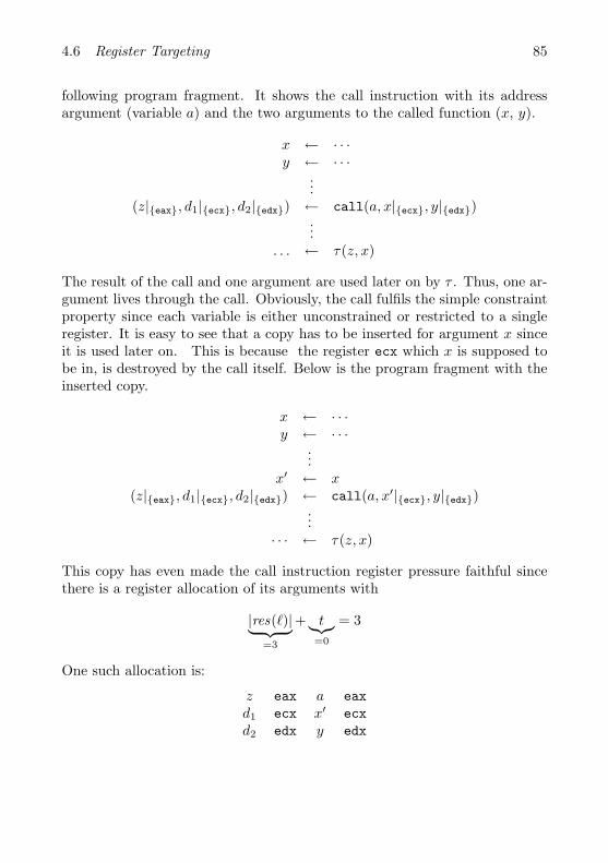
4.6 Register Targeting 85
following program fragment. It shows the call instruction with its addressargument (variable a) and the two arguments to the called function (x, y).
x ← · · ·y ← · · ·
...(z|{eax}, d1|{ecx}, d2|{edx}) ← call(a, x|{ecx}, y|{edx})
.... . . ← τ(z, x)
The result of the call and one argument are used later on by τ . Thus, one ar-gument lives through the call. Obviously, the call fulfils the simple constraintproperty since each variable is either unconstrained or restricted to a singleregister. It is easy to see that a copy has to be inserted for argument x sinceit is used later on. This is because the register ecx which x is supposed tobe in, is destroyed by the call itself. Below is the program fragment with theinserted copy.
x ← · · ·y ← · · ·
...x′ ← x
(z|{eax}, d1|{ecx}, d2|{edx}) ← call(a, x′|{ecx}, y|{edx})...
· · · ← τ(z, x)
This copy has even made the call instruction register pressure faithful sincethere is a register allocation of its arguments with
|res(`)|︸ ︷︷ ︸=3
+ t︸︷︷︸=0
= 3
One such allocation is:
z eax a eaxd1 ecx x′ ecxd2 edx y edx

86 SSA Register Allocation
5 Implementation and Evaluation
We conducted various measurements to show the competitiveness of the reg-ister allocator presented in this thesis. Since the pre-spilling heuristics aspresented in Section 3.1.5.2 are sufficient, our allocator will never introduceadditional spill code after spilling has happened. Thus, concerning spilling,the presented allocator is at least as good as any other allocator available,since it can use the same register-pressure-based spilling methods. The mainquestion arising from this paradigm, is whether the live range splitting im-plied by Φ-operations and register constraints causes significant performancepenalties. Thus, we chose the x86 architecture for measurements since it isknown to possess many irregularly constrained instructions. Therefore , weexpect a large amount of live range splits due to these constraints.
Before presenting the results of the experimental investigation, we describethe compiler used to conduct the measurements.
5.1 Implementation
We implemented the register allocator described in the previous chapter intothe C compiler developed at the Institut fur Programmstrukturen und Datenor-ganisation at the Universitat Karlsruhe. This compiler is built upon Firm(see Lindenmaier et al. [2005]), a graph-based SSA intermediate representa-tion which is similar to the Sea of Nodes IR described by Click and Paleczny[1995].
5.1.1 The Firm Backend
Based on the IR Firm, we implemented a completely SSA-based backend.After all architecture independent optimizations in the compiler’s “middleend” have been finished, the code represented by data and control flow graphs
87
88 Implementation and Evaluation
gets lowered successively. Firstly we implement the rules of the applicationbinary interface (ABI). This comprises building stack frames, deciding whichparameters of function calls will reside in registers or on the stack and soon. Afterwards, the architecture independent IR nodes are replaced by nodesrepresenting machine instructions.
As register allocation requires a totally ordered instruction sequence tocompute liveness (and thus interference) correctly, the data dependence graphsinside the basic blocks are scheduled using a common latency based listscheduling algorithm as described in Muchnick [1998].1
Now register allocation takes place. The allocation is performed separatelyfor each register class. As described in the previous chapter, the registerallocator runs in several phases:
1. Copy instructions for constrained instructions are inserted to make theregister pressure match the actual register demand (see Section 4.6).
2. Spilling is performed using the heuristic described in Section 3.1.5.2 andthe book of [Morgan, 1998, page 319]. It is adapted using the methodsdescribed in Section 4.2.1.
3. Then live range splits for constraint handling are inserted (see Sec-tion 4.6.3) and registers are assigned to the variables (see Section 4.3)
4. Afterwards, coalescing runs as an (optional) optimization of the coloring,trying to remove as many move instructions as possible.
5. Φ-operations are implemented as described in Section 4.4 and the as-sembly text file is emitted.
5.1.2 The x86 Architecture
In this section we describe how the features of the x86 are displayed to theregister allocator. Due to its long history, the x86 architecture exhibits sig-nificant differences compared to standard RISC architectures. We will brieflypresent the features which deserve special treatment:
1. x86 processors provide eight 32-bit integer registers. One register (esp)is reserved as the stack pointer and is hence excluded from registerallocation. The other registers are called eax, ebx, ecx, edx, esi, ediand ebp. Most instructions also allow to access the lower 16 bit of
1Future implementations could enhance the scheduling algorithm by heuristics whichkeep track of the register pressure as described in Hoxey et al. [1996].
5.1 Implementation 89
eax,. . . ,ebp through aliased registers ax,. . . ,bp. The lower 16 bit ofeax,. . . ,edx can also be accessed in 8 bit portions through registersal,ah,. . . ,dl,dh.
2. Almost all binary instructions use 2-address code, i.e. the first operandof the instruction is also the target of the instruction. Thus, if the firstoperand is assigned to register eax the result of the operation is writtento eax.
3. Several instructions exhibit register constraints. For the argument aswell as the result registers. Mostly, these constraints demand that anargument or result must reside in a specific register.
4. The floating point registers are organized as a stack. Most instructionsimplicitly use the top of the stack (TOS) as operand and result. Thus,registers cannot be assigned directly to floating point variables.
We address these irregularities as follows:
5.1.2.1 Aliased Registers
C dictates that all char and short operands are casted to int in integercomputations and as an int is 32-bit wide in our compiler, most integeroperations will be 32-bit operations. Thus, we do not support access to thealiased register parts of the integer registers. This sometimes leads to slightlyslower code since narrowing results in additional mask instructions thatclear the respective bits.
5.1.2.2 2-Address Code
If the operand variable assigned to the target register becomes dead at thatlabel in question, 2-address code can be seen as a kind of code compressionsince the instruction word needs to store only two registers. But if thatoperand (let us call it the overwritten operand) lives past the instruction ithas to be copied to the result register before the instruction.2 However, this“trick” bears a subtle problem. Consider a non-commutative operation suchas sub and a label
` : z ← sub(x, y)
2Note that these copies can be optimized away by the coalescing phase if they are notnecessary.
90 Implementation and Evaluation
where x lives through ` and y dies at `. Assume, the register allocator pro-duced a register allocation where ρ(z) = ρ(y) = eax and ρ(x) = ebx. Thenusing the “copy trick” would result in the following code sequence destroyingthe contents of eax before it is used:
x′ : eax ← x : ebxz : eax ← sub(x′ : eax, y : eax)
Some instructions such as sub can be re-formulated to circumvent this diffi-culty. In the example above, one could write
x′ : eax ← neg(x : eax)z : eax ← add(x′ : eax, y : ebx)
thereby making the dying operand the overwritten one. However, for themost non-commutative instructions this is not possible. Therefore, for non-commutative operations we have to ensure that the result register is differentfrom the register assigned to the overwritten operand. This is achieved byadding an artificial use after the label which forces this operand to live throughthe label. Then the not overwritten operand interferes with the result andnever gets assigned the same register. Concerning our example above thisyields the following code:
` : z ← sub(x, y)use(y)
Note that this artificial use can be omitted if both operands are the same.Furthermore, if the overwritten operand dies at the label and the second onelives through it a third register is needed. Thus, 2-address code can causeadditional register pressure.
5.1.2.3 Register Constraints
Almost all constrained instructions require that an operand (or result) mustreside in one specific register. Examples are shown in the table below.
Instruction Constraintsmultiplication one operand must be in eax; result is in edx:eax
division 64-bit operand and result must be in edx:eaxshift and rotate shift count must be in register ecx
byte load result is 8-bit register, i.e. one of eax, . . . , edx
5.2 Measurements 91
Besides the byte loads, all constrained x86 instructions only exhibit con-straints to single registers. For byte loads, only the subset eax, . . . , edxis admissible. To fulfill the single constraints property (see Section 4.6.1),one of these registers can be arbitrarily selected. However, our coalescingalgorithms (see 4.5) can take all admissible registers into account.
5.1.2.4 Stack-based FPU
Leung and George [2001] describe an approach which allows to assign vir-tual registers to the floating point variables and turn them into FPU stackoperands afterwards. Alternatively, on more modern incarnations of the x86architecture, the SSE2 instruction set is available which allows to performdouble precision floating point arithmetic in the lower halves of eight 128-bitvector registers.
5.2 Measurements
In principle, k-colorable chordal graphs can by colored optimally with thesimplify/select-scheme.3 Since the original allocator presented by Chaitinmerges nodes in the coalescing phase, spills might be introduced in favor ofcopies, which is unacceptable. This cannot happen using conservative coa-lescing allocators. However, they remove far too few copies (see Section 3.1.1and Appel and George [2001]) due to their conservative heuristic. We alsoexperimented with Park and Moon’s optimistic register coalescing (see Sec-tion 3.1.1) that is able to undo some coalescings. We found that it frequentlyinserted spills into the k-colorable chordal IGs. This is mainly because it canonly undo the coalescing of the node that is currently to be colored. If thecoloring for a node fails due to already colored coalesced nodes their coalesc-ing cannot be undone. This results in current allocators either inserting spillsin favor of copies or removing far too few copies to prevent spills from beinginserted.
In comparison to existing, non-SSA register allocators our allocator willnot add a single spill after a pressure-based spilling algorithm has run. Sincethese spilling heuristics are also applied by conventional register allocators, wenever insert more spills than a conventional allocator using the same pressure-based spilling heuristic. Hence, our investigations concentrate on the overheadcaused by the live range splitting due to Φ-operations, spilling and register
3A chordal graph always has a simplicial node and simplicial nodes have insignificantdegree, so there is always a node available for elimination.
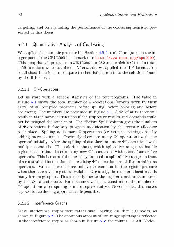
92 Implementation and Evaluation
targeting, and on evaluating the performance of the coalescing heuristic pre-sented in this thesis.
5.2.1 Quantitative Analysis of Coalescing
We applied the heuristic presented in Section 4.5.2 to all C programs in the in-teger part of the CPU2000 benchmark (see http://www.spec.org/cpu2000).This comprises all programs in CINT2000 but 252.eon which is C++. In total,4459 functions were examined. Afterwards, we applied the ILP formulationto all those functions to compare the heuristic’s results to the solutions foundby the ILP solver.
5.2.1.1 Φr-Operations
Let us start with a general statistics of the test programs. The table inFigure 5.1 shows the total number of Φr-operations (broken down by theirarity) of all compiled programs before spilling, before coloring and beforecoalescing. The numbers are presented in Figure 5.1. A Φr of arity three willresult in three move instructions if the respective results and operands couldnot be assigned the same color. The “Before Spill” column gives the numbersof Φ-operations before any program modification by the register allocatortook place. Spilling adds more Φ-operations (or extends existing ones byadding more columns). Obviously there are many Φr-operations with oneoperand initially. After the spilling phase there are more Φr-operations withmultiple operands. The coloring phase, which splits live ranges to handleregister constraints, inserts many new Φr-operations with about four or fiveoperands. This is reasonable since they are used to split all live ranges in frontof a constrained instruction, the resulting Φr-operation has all live variables asoperands. Values between three and five are common for the register pressurewhen there are seven registers available. Obviously, the register allocator addsmany live range splits. This is mostly due to the register constraints imposedby the x86 architecture. For machines with few constraints, the number ofΦr-operations after spilling is more representative. Nevertheless, this makesa powerful coalescing approach indispensable.
5.2.1.2 Interference Graphs
Most interference graphs were rather small having less than 500 nodes, asshown in Figure 5.2. The enormous amount of live range splitting is reflectedin the interference graphs as shown in Figure 5.3: the column “∅ Aff. Nodes”
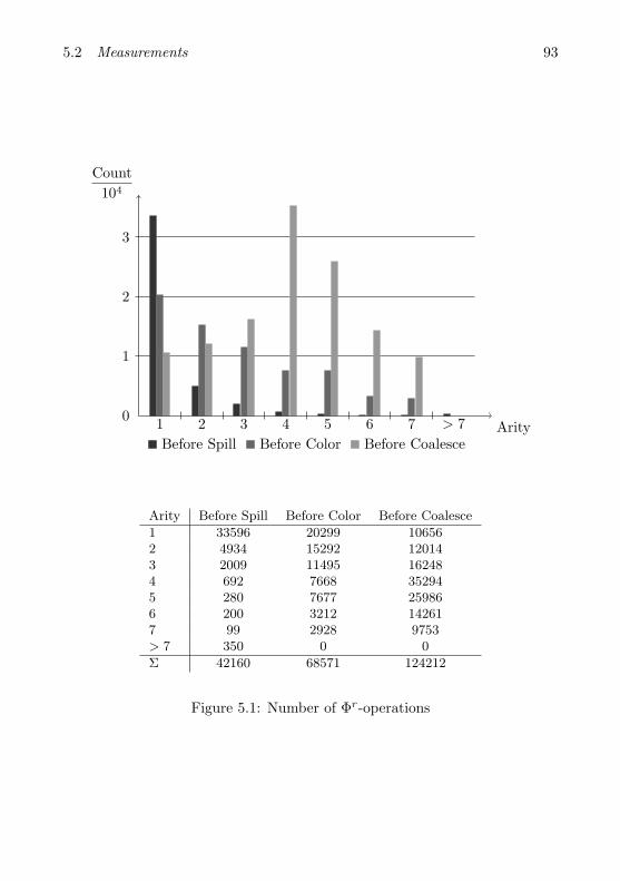
5.2 Measurements 93
0
1
2
3
1 2 3 4 5 6 7 > 7
Count104
ArityBefore Spill Before Color Before Coalesce
Arity Before Spill Before Color Before Coalesce
1 33596 20299 106562 4934 15292 120143 2009 11495 162484 692 7668 352945 280 7677 259866 200 3212 142617 99 2928 9753> 7 350 0 0
Σ 42160 68571 124212
Figure 5.1: Number of Φr-operations
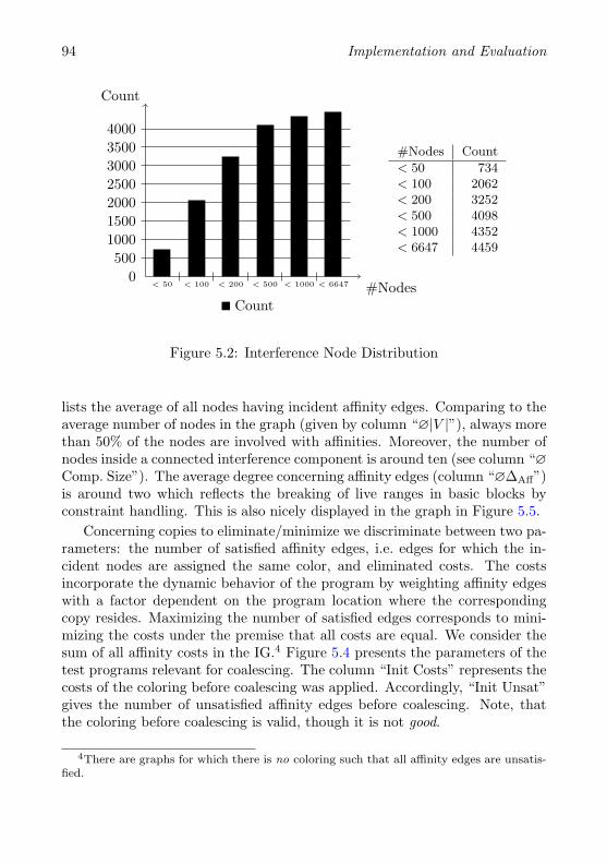
94 Implementation and Evaluation
0500
1000150020002500300035004000
< 50 < 100 < 200 < 500 < 1000 < 6647
Count
#NodesCount
#Nodes Count
< 50 734< 100 2062< 200 3252< 500 4098< 1000 4352< 6647 4459
Figure 5.2: Interference Node Distribution
lists the average of all nodes having incident affinity edges. Comparing to theaverage number of nodes in the graph (given by column “∅|V |”), always morethan 50% of the nodes are involved with affinities. Moreover, the number ofnodes inside a connected interference component is around ten (see column “∅Comp. Size”). The average degree concerning affinity edges (column “∅∆Aff”)is around two which reflects the breaking of live ranges in basic blocks byconstraint handling. This is also nicely displayed in the graph in Figure 5.5.
Concerning copies to eliminate/minimize we discriminate between two pa-rameters: the number of satisfied affinity edges, i.e. edges for which the in-cident nodes are assigned the same color, and eliminated costs. The costsincorporate the dynamic behavior of the program by weighting affinity edgeswith a factor dependent on the program location where the correspondingcopy resides. Maximizing the number of satisfied edges corresponds to mini-mizing the costs under the premise that all costs are equal. We consider thesum of all affinity costs in the IG.4 Figure 5.4 presents the parameters of thetest programs relevant for coalescing. The column “Init Costs” represents thecosts of the coloring before coalescing was applied. Accordingly, “Init Unsat”gives the number of unsatisfied affinity edges before coalescing. Note, thatthe coloring before coalescing is valid, though it is not good.
4There are graphs for which there is no coloring such that all affinity edges are unsatis-fied.
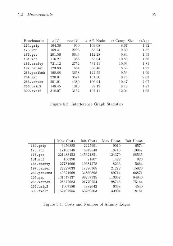
5.2 Measurements 95
Benchmarks ∅ |V | max |V | ∅ Aff. Nodes ∅ Comp. Size ∅∆Aff
164.gzip 164.38 930 109.08 8.67 1.92175.vpr 169.41 2293 85.24 9.30 1.82176.gcc 201.56 6646 112.28 9.84 1.95181.mcf 116.27 388 65.04 10.80 1.68186.crafty 721.12 2752 534.41 10.96 1.81197.parser 123.83 1684 68.48 8.53 1.92253.perlbmk 198.88 3658 122.55 9.53 1.99254.gap 220.01 3574 151.50 9.75 2.03255.vortex 201.01 4380 106.94 10.47 2.07256.bzip2 148.45 1016 92.12 8.43 1.87300.twolf 318.07 3152 197.11 12.04 1.65
Figure 5.3: Interference Graph Statistics
Max Costs Init Costs Max Unsat Init Unsat
164.gzip 3456885 2225991 9010 6574175.vpr 17105748 6949543 18716 13057176.gcc 221483452 145321851 124379 88535181.mcf 136390 71807 1422 928186.crafty 27781660 19681278 8233 5664197.parser 22227033 17270365 21272 15828253.perlbmk 49321969 34860898 89714 66871254.gap 131547137 89237335 113067 84846255.vortex 28572683 21770254 98745 75164256.bzip2 7007580 4882642 6368 4540300.twolf 162497955 63259503 30904 18151
Figure 5.4: Costs and Number of Affinity Edges
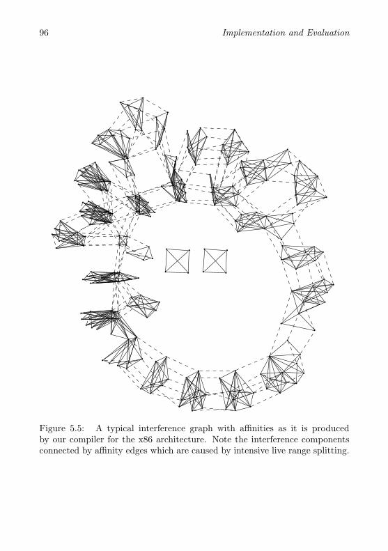
96 Implementation and Evaluation
Figure 5.5: A typical interference graph with affinities as it is producedby our compiler for the x86 architecture. Note the interference componentsconnected by affinity edges which are caused by intensive live range splitting.
5.2 Measurements 97
5.2.1.3 The Coalescing Heuristic
To improve their coloring with respect to affinity costs, all IGs were processedby coalescing heuristic presented in Section 4.5.2. The results are displayedin Figure 5.6. The diagram shows three columns per benchmark. The blackone shows the maximal costs of all IGs in the respective benchmark. Thedark grey column “Init” shows the costs before coloring and the light grayone “Heuristic” shows the costs after the coalescing heuristic ran. The tablein Figure 5.6 also lists the number of unsatisfied affinity edges after coalesc-ing (“After Unsat”) and the percentage with respect to the total number ofaffinity edges (“%After Unsat”). The column “%After Costs” gives the per-centage of affinity costs present in the IG after coalescing. We can see thatthe percentage of costs that are eliminated by the heuristic ranges from 91%to 98%. Hence, the presented heuristic is a reasonable means to eliminatemost of the copies inserted due to live range splitting. Figure 5.7 shows theruntime distribution of the coalescing heuristic. For 80% percent of all inter-ference graphs the heuristic takes less than 500ms to run. It should be notedthat the heuristic is written in Java and the compiler is implemented in C.This runtime includes the transfer of the interference information from C toJava. A pure C implementation would surely be faster.
5.2.1.4 ILP Coalescing
To better assess the quality of the coalescing heuristic we applied an ILPsolver to all benchmark programs.5 We used the ILP formulation presentedin Section 4.5.3 and set the time limit for the solver to five minutes. Priorto the ILP, we ran the heuristic on the graph and provided its solution as astart value to the ILP solver. Hence, the solver did not need to spend time onsearching a feasible solution in the beginning. Out of 4459 problems, only 211were not solved optimally within this time. In those cases we also recordedthe best lower bound (abbreviated BB in the following) known to the solverafter five minutes. The optimal solution of a problem lies between BB and theobjective value returned. However, a common observation in practice is thatthe solver starts lowering the objective value6 and then remains a long time atthe same best solution, only raising the lower bound. Therefore, there mightbe problems among the 211 non-optimal ones, for which the ILP solution isoptimal but the solver failed to prove it within the time limit.
5The solver was CPLEX 9.1 (see http://www.ilog.com) on a 2.4Ghz Pentium with 1GBmain memory.
6Note that we expressed coalescing as a minimization problem
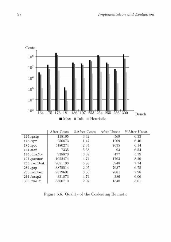
98 Implementation and Evaluation
103
104
105
106
107
108
164 175 176 181 186 197 253 254 255 256 300
Costs
BenchMax Init Heuristic
After Costs %After Costs After Unsat %After Unsat
164.gzip 118165 3.42 569 6.32175.vpr 250873 1.47 1209 6.46176.gcc 5180274 2.34 7635 6.14181.mcf 7335 5.38 93 6.54186.crafty 938870 3.38 477 5.79197.parser 1052474 4.74 1763 8.29253.perlbmk 2651188 5.38 6948 7.74254.gap 3875514 2.95 7637 6.75255.vortex 2379601 8.33 7881 7.98256.bzip2 331873 4.74 386 6.06300.twolf 3360710 2.07 1548 5.01
Figure 5.6: Quality of the Coalescing Heuristic
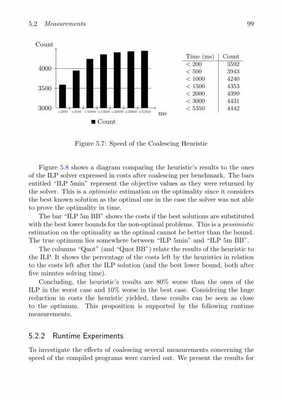
5.2 Measurements 99
3000
3500
4000
<200 <500 <1000 <1500 <2000 <3000 <5350
Count
msCount
Time (ms) Count
< 200 3592< 500 3943< 1000 4240< 1500 4353< 2000 4399< 3000 4431< 5350 4442
Figure 5.7: Speed of the Coalescing Heuristic
Figure 5.8 shows a diagram comparing the heuristic’s results to the onesof the ILP solver expressed in costs after coalescing per benchmark. The barsentitled “ILP 5min” represent the objective values as they were returned bythe solver. This is a optimistic estimation on the optimality since it considersthe best known solution as the optimal one in the case the solver was not ableto prove the optimality in time.
The bar “ILP 5m BB” shows the costs if the best solutions are substitutedwith the best lower bounds for the non-optimal problems. This is a pessimisticestimation on the optimality as the optimal cannot be better than the bound.The true optimum lies somewhere between “ILP 5min” and “ILP 5m BB”.
The columns “Quot” (and “Quot BB”) relate the results of the heuristic tothe ILP. It shows the percentage of the costs left by the heuristics in relationto the costs left after the ILP solution (and the best lower bound, both afterfive minutes solving time).
Concluding, the heuristic’s results are 80% worse than the ones of theILP in the worst case and 10% worse in the best case. Considering the hugereduction in costs the heuristic yielded, these results can be seen as closeto the optimum. This proposition is supported by the following runtimemeasurements.
5.2.2 Runtime Experiments
To investigate the effects of coalescing several measurements concerning thespeed of the compiled programs were carried out. We present the results for
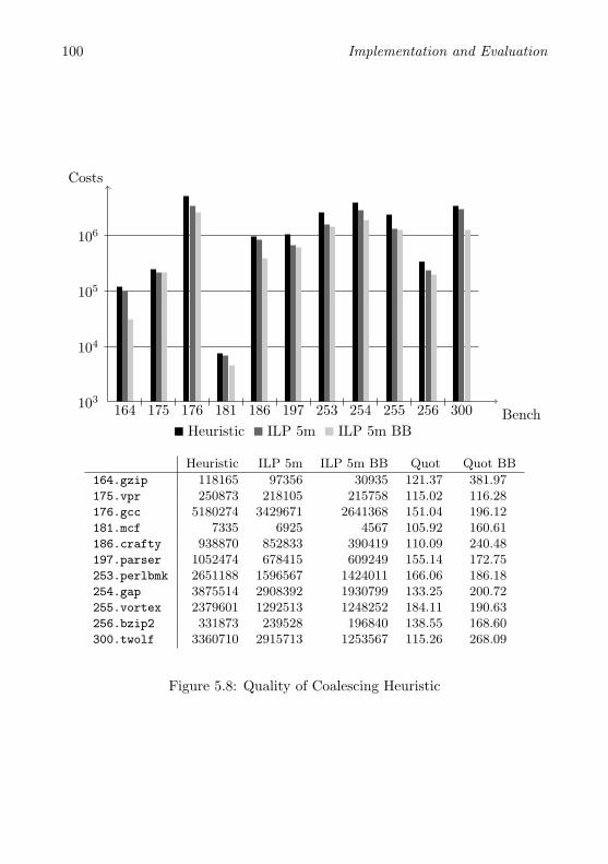
100 Implementation and Evaluation
103
104
105
106
164 175 176 181 186 197 253 254 255 256 300
Costs
BenchHeuristic ILP 5m ILP 5m BB
Heuristic ILP 5m ILP 5m BB Quot Quot BB
164.gzip 118165 97356 30935 121.37 381.97175.vpr 250873 218105 215758 115.02 116.28176.gcc 5180274 3429671 2641368 151.04 196.12181.mcf 7335 6925 4567 105.92 160.61186.crafty 938870 852833 390419 110.09 240.48197.parser 1052474 678415 609249 155.14 172.75253.perlbmk 2651188 1596567 1424011 166.06 186.18254.gap 3875514 2908392 1930799 133.25 200.72255.vortex 2379601 1292513 1248252 184.11 190.63256.bzip2 331873 239528 196840 138.55 168.60300.twolf 3360710 2915713 1253567 115.26 268.09
Figure 5.8: Quality of Coalescing Heuristic
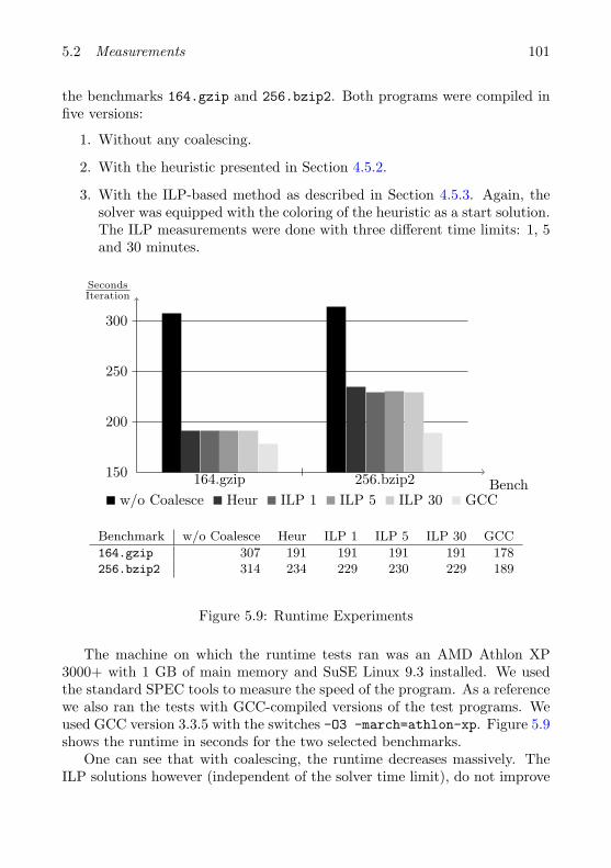
5.2 Measurements 101
the benchmarks 164.gzip and 256.bzip2. Both programs were compiled infive versions:
1. Without any coalescing.
2. With the heuristic presented in Section 4.5.2.
3. With the ILP-based method as described in Section 4.5.3. Again, thesolver was equipped with the coloring of the heuristic as a start solution.The ILP measurements were done with three different time limits: 1, 5and 30 minutes.
150
200
250
300
164.gzip 256.bzip2
SecondsIteration
Benchw/o Coalesce Heur ILP 1 ILP 5 ILP 30 GCC
Benchmark w/o Coalesce Heur ILP 1 ILP 5 ILP 30 GCC
164.gzip 307 191 191 191 191 178256.bzip2 314 234 229 230 229 189
Figure 5.9: Runtime Experiments
The machine on which the runtime tests ran was an AMD Athlon XP3000+ with 1 GB of main memory and SuSE Linux 9.3 installed. We usedthe standard SPEC tools to measure the speed of the program. As a referencewe also ran the tests with GCC-compiled versions of the test programs. Weused GCC version 3.3.5 with the switches -O3 -march=athlon-xp. Figure 5.9shows the runtime in seconds for the two selected benchmarks.
One can see that with coalescing, the runtime decreases massively. TheILP solutions however (independent of the solver time limit), do not improve

102 Implementation and Evaluation
the runtime significantly. The good values for GCC are mainly due to otherdeficiencies in our compiler, such as bad scheduling leading to many spills orlack of other optimizations such as loop unrolling and aggressive exploitationof machine features.
6 Conclusions and Future Work
6.1 Conclusions
In this thesis we present a novel approach of performing register allocation onthe SSA form. Our main contribution is the proof that interference graphsof SSA-form programs are chordal. This theoretical result has far reachingconsequences for the architecture of global register allocators which we com-prehensively cover in this thesis:
• Pressure based spilling heuristics as they are commonly used are nowsufficient to make the interference graph colorable. No further spills willbe introduced by the coloring phase. This allows to consider coloringand spilling separately, which is an enormous simplification to registerallocation since the expensive iterative approach used in most globalgraph-coloring register allocators can be abandoned.
• We provide a thorough analysis of the register targeting problem as itoccurs in all contemporary runtime systems and processor architectures.We show, that for general register constraints, register allocation is NP-complete even for a single constrained instruction in one basic block.Based on this result, we consider a restricted version of the targetingproblem and show how it can be seamlessly integrated in our registerallocator framework.
• We show that coloring the interference graph can actually be done with-out constructing the graph itself. This is very important for scenarioswhere compile speed matters, such as Just-In-Time compilers, as inter-ference graphs are usually complex data structures that are tedious toadminister.
• As our maxim is to never make spills in favor of copies, the elimination
103
104 Conclusions and Future Work
of copies (coalescing) may never be allowed to turn a valid coloringinto an invalid one. Thus, we express coalescing as an optimizationproblem over interference graphs: find not only a valid coloring buta good one with respect to copy costs. Thereby, we take care thatthe interference graph itself is never modified to preserve its chordality;the only thing that changes is its coloring. Furthermore, we describeefficient ways how coalescing algorithms can query the interference graphwithout materializing it as a data structure.
After laying the theoretical foundations, we evaluate our approach usinga modern C compiler targeted at the x86 architecture. Hereby, our focus isdirected on the quality of the proposed coalescing methods. As constrainedinstructions appear frequently in the code for x86 processors, a lot of live rangesplitting is performed by our allocator. As our runtime experiments show, thismakes coalescing crucial as it reduces the runtime of the test programs by 40%.
Furthermore, as the evaluation shows, the proposed coalescing heuristicdelivered solutions which are very close (between 10% and 80% worse) to theones found by an ILP solver. These ILP solutions were proven to be optimalin 95% of all compiled functions. Concerning the runtime of the compiled pro-grams, the better solutions of the ILP solver provide only marginal speedup.Hence, the proposed heuristic provides very good results.
6.2 Future Work
Future research in this area could include the following topics:
• We experimented with machines with few registers. Evaluating thisallocator for machines with more registers (especially newer DSPs with64 or 128 registers) is desirable. Especially the effects of having a largeregister file on coalescing have to be investigated.
• Our copy minimization problem only takes into account the given loca-tions for the live range splits. It is not capable of moving copies to otherplaces in the program. However, allowing live range splits at arbitrarylocations could result in lower total costs.
• The integration of more complicated register targeting issues like pairedregisters and aliased registers is important especially for DSPs.
• The potential compile time benefits of SSA-based register allocationcould be investigated in Just-In-Time compilation scenarios.
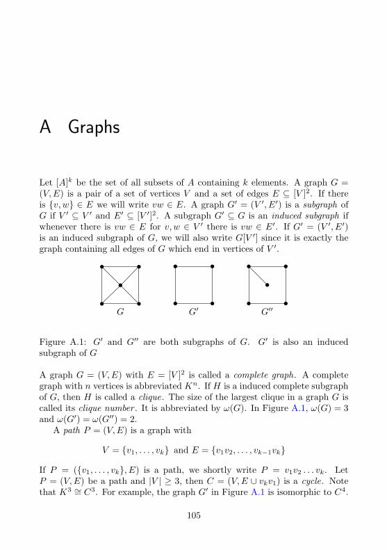
A Graphs
Let [A]k be the set of all subsets of A containing k elements. A graph G =(V,E) is a pair of a set of vertices V and a set of edges E ⊆ [V ]2. If thereis {v, w} ∈ E we will write vw ∈ E. A graph G′ = (V ′, E′) is a subgraph ofG if V ′ ⊆ V ′ and E′ ⊆ [V ′]2. A subgraph G′ ⊆ G is an induced subgraph ifwhenever there is vw ∈ E for v, w ∈ V ′ there is vw ∈ E′. If G′ = (V ′, E′)is an induced subgraph of G, we will also write G[V ′] since it is exactly thegraph containing all edges of G which end in vertices of V ′.
G G′ G′′
Figure A.1: G′ and G′′ are both subgraphs of G. G′ is also an inducedsubgraph of G
A graph G = (V,E) with E = [V ]2 is called a complete graph. A completegraph with n vertices is abbreviated Kn. If H is a induced complete subgraphof G, then H is called a clique. The size of the largest clique in a graph G iscalled its clique number . It is abbreviated by ω(G). In Figure A.1, ω(G) = 3and ω(G′) = ω(G′′) = 2.
A path P = (V,E) is a graph with
V = {v1, . . . , vk} and E = {v1v2, . . . , vk−1vk}
If P = ({v1, . . . , vk}, E) is a path, we shortly write P = v1v2 . . . vk. LetP = (V,E) be a path and |V | ≥ 3, then C = (V,E ∪ vkv1) is a cycle. Notethat K3 ∼= C3. For example, the graph G′ in Figure A.1 is isomorphic to C4.
105
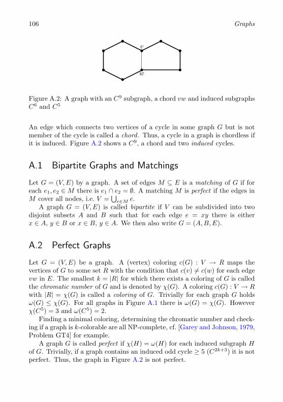
106 Graphs
v
w
Figure A.2: A graph with an C9 subgraph, a chord vw and induced subgraphsC6 and C5
An edge which connects two vertices of a cycle in some graph G but is notmember of the cycle is called a chord . Thus, a cycle in a graph is chordless ifit is induced. Figure A.2 shows a C9, a chord and two induced cycles.
A.1 Bipartite Graphs and Matchings
Let G = (V,E) by a graph. A set of edges M ⊆ E is a matching of G if foreach e1, e2 ∈M there is e1 ∩ e2 = ∅. A matching M is perfect if the edges inM cover all nodes, i.e. V =
⋃e∈M e.
A graph G = (V,E) is called bipartite if V can be subdivided into twodisjoint subsets A and B such that for each edge e = xy there is eitherx ∈ A, y ∈ B or x ∈ B, y ∈ A. We then also write G = (A,B, E).
A.2 Perfect Graphs
Let G = (V,E) be a graph. A (vertex) coloring c(G) : V → R maps thevertices of G to some set R with the condition that c(v) 6= c(w) for each edgevw in E. The smallest k = |R| for which there exists a coloring of G is calledthe chromatic number of G and is denoted by χ(G). A coloring c(G) : V → Rwith |R| = χ(G) is called a coloring of G. Trivially for each graph G holdsω(G) ≤ χ(G). For all graphs in Figure A.1 there is ω(G) = χ(G). Howeverχ(C5) = 3 and ω(C5) = 2.
Finding a minimal coloring, determining the chromatic number and check-ing if a graph is k-colorable are all NP-complete, cf. [Garey and Johnson, 1979,Problem GT4] for example.
A graph G is called perfect if χ(H) = ω(H) for each induced subgraph Hof G. Trivially, if a graph contains an induced odd cycle ≥ 5 (C2k+3) it is notperfect. Thus, the graph in Figure A.2 is not perfect.
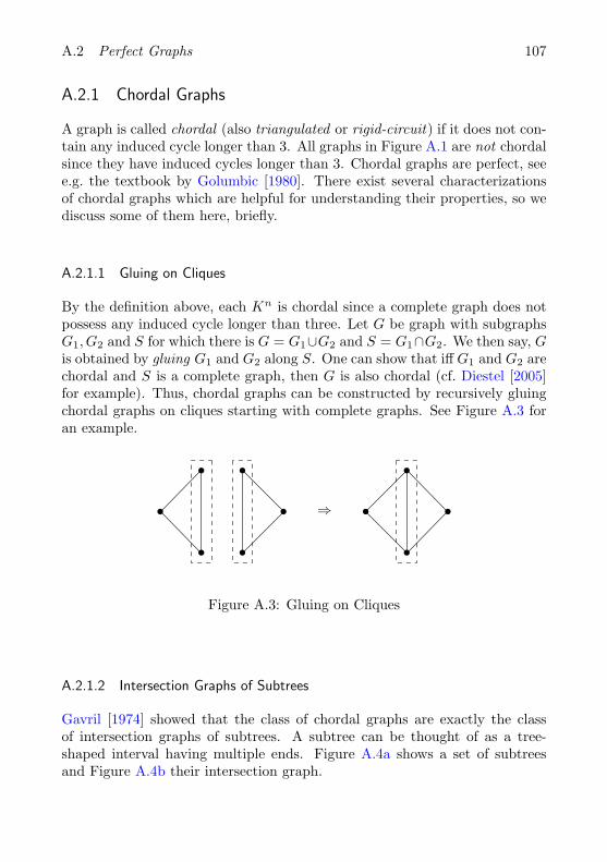
A.2 Perfect Graphs 107
A.2.1 Chordal Graphs
A graph is called chordal (also triangulated or rigid-circuit) if it does not con-tain any induced cycle longer than 3. All graphs in Figure A.1 are not chordalsince they have induced cycles longer than 3. Chordal graphs are perfect, seee.g. the textbook by Golumbic [1980]. There exist several characterizationsof chordal graphs which are helpful for understanding their properties, so wediscuss some of them here, briefly.
A.2.1.1 Gluing on Cliques
By the definition above, each Kn is chordal since a complete graph does notpossess any induced cycle longer than three. Let G be graph with subgraphsG1, G2 and S for which there is G = G1∪G2 and S = G1∩G2. We then say, Gis obtained by gluing G1 and G2 along S. One can show that iff G1 and G2 arechordal and S is a complete graph, then G is also chordal (cf. Diestel [2005]for example). Thus, chordal graphs can be constructed by recursively gluingchordal graphs on cliques starting with complete graphs. See Figure A.3 foran example.
⇒
Figure A.3: Gluing on Cliques
A.2.1.2 Intersection Graphs of Subtrees
Gavril [1974] showed that the class of chordal graphs are exactly the classof intersection graphs of subtrees. A subtree can be thought of as a tree-shaped interval having multiple ends. Figure A.4a shows a set of subtreesand Figure A.4b their intersection graph.
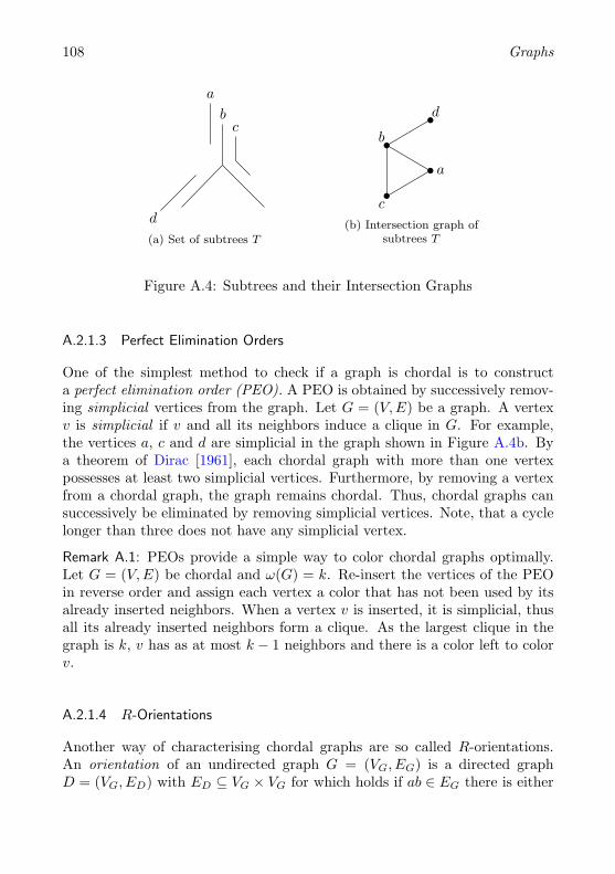
108 Graphs
a
bc
d
(a) Set of subtrees T
a
b
c
d
(b) Intersection graph ofsubtrees T
Figure A.4: Subtrees and their Intersection Graphs
A.2.1.3 Perfect Elimination Orders
One of the simplest method to check if a graph is chordal is to constructa perfect elimination order (PEO). A PEO is obtained by successively remov-ing simplicial vertices from the graph. Let G = (V,E) be a graph. A vertexv is simplicial if v and all its neighbors induce a clique in G. For example,the vertices a, c and d are simplicial in the graph shown in Figure A.4b. Bya theorem of Dirac [1961], each chordal graph with more than one vertexpossesses at least two simplicial vertices. Furthermore, by removing a vertexfrom a chordal graph, the graph remains chordal. Thus, chordal graphs cansuccessively be eliminated by removing simplicial vertices. Note, that a cyclelonger than three does not have any simplicial vertex.
Remark A.1: PEOs provide a simple way to color chordal graphs optimally.Let G = (V,E) be chordal and ω(G) = k. Re-insert the vertices of the PEOin reverse order and assign each vertex a color that has not been used by itsalready inserted neighbors. When a vertex v is inserted, it is simplicial, thusall its already inserted neighbors form a clique. As the largest clique in thegraph is k, v has as at most k − 1 neighbors and there is a color left to colorv.
A.2.1.4 R-Orientations
Another way of characterising chordal graphs are so called R-orientations.An orientation of an undirected graph G = (VG, EG) is a directed graphD = (VG, ED) with ED ⊆ VG × VG for which holds if ab ∈ EG there is either

A.2 Perfect Graphs 109
(a, b) ∈ ED or (b, a) ∈ ED. An R-orientation D of an undirected graph G isan orientation which further fulfills following properties:
1. D contains no directed cycles
2. If (b, a) ∈ ED and (c, a) ∈ ED then there is bc ∈ EG, i.e. (b, c) ∈ ED or(c, b) ∈ RD.
Rose [1970] shows that the graphs possessing an R-orientation are chordaland vice versa.

110 Graphs
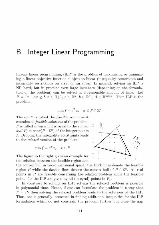
B Integer Linear Programming
Integer linear programming (ILP) is the problem of maximizing or minimiz-ing a linear objective function subject to linear (in)equality constraints andintegrality restrictions on a set of variables. In general, solving an ILP isNP hard, but in practice even large instances (depending on the formula-tion of the problem) can be solved in a reasonable amount of time. LetP = {x | Ax ≥ b, x ∈ Rn
+}, c ∈ Rn, b ∈ Rm, A ∈ Rm×n. Then ILP is theproblem:
min f = cT x, x ∈ P ∩ Zn
cut
PPI
I
The set P is called the feasible region as itcontains all feasible solutions of the problem.P is called integral if it is equal to the convexhull PI = conv(P ∩Zn) of the integer pointsI. Droping the integrality constraints leadsto the relaxed version of the problem:
min f = cT x, x ∈ P
The figure to the right gives an example forthe relation between the feasible region andthe convex hull in two-dimensional space: the thick lines denote the feasibleregion P while the dashed lines denote the convex hull of P ∩ Zn. All realpoints in P are feasible concerning the relaxed problem while the feasiblepoints for the ILP are given by all (integral) points in PI .
In constrast to solving an ILP, solving the relaxed problem is possiblein polynomial time. Hence, if one can formulate the problem in a way thatP = PI then solving the relaxed problem leads to the solutions of the ILP.Thus, one is generally interested in finding additional inequalties for the ILPformulation which do not constrain the problem further but close the gap
111

112 Integer Linear Programming
between the feasible region and the convex hull. Such inequalities are calledcuts. In our example, the dotted line represents a cut. Cuts are generally amean to provide the solver with more information of the problem’s structure sothat it can discard infeasible solutions more quickly. For an in-depth coverageon (I)LP we refer to Schrijver [1986], Nemhauser and Wolsey [1988].
Bibliography
C. Andersson. Register Allocation by Optimal Graph Coloring. In G. Hedin,editor, CC 2003, volume 2622 of LNCS, pages 33–45, Heidelberg, 2003.Springer-Verlag.
A. Appel and L. George. Optimal Coalescing Challenge. Website, August2000. URL http://www.cs.princeton.edu/∼appel/coalesce/.
A. W. Appel and L. George. Optimal Spilling for CISC Machines with FewRegisters. In ACM SIGPLAN 2001 Conference on Programming LanguageDesign and Implementation, pages 243–253, June 2001.
A. W. Appel and J. Palsberg. Modern Compiler Implementation in Java.Cambridge University Press, second edition, 2002.
L. Belady. A Study of Replacement of Algorithms for a Virtual StorageComputer. IBM Systems Journal, 5:78–101, 1966.
M. Biro, M. Hujter, and Z. Tuza. Precoloring extension. I. Interval Graphs.Discrete Mathematics, 100:267–279, 1992.
F. Bouchez, A. Darte, C. Guillon, and F. Rastello. Register Allocation andSpill Complexity under SSA. Technical Report 2005-33, ENS-Lyon, Aug2005.
P. Briggs. Register Allocation via Graph Coloring. PhD thesis, Rice University,April 1992.
P. Briggs, K. D. Cooper, and L. Torczon. Improvements to Graph ColoringRegister Allocation. ACM Trans. Program. Lang. Syst., 16(3):428–455,1994. ISSN 0164-0925. doi: http://doi.acm.org/10.1145/177492.177575.
113
114 Bibliography
P. Brisk, F. Dabiri, J. Macbeth, and M. Sarrafzadeh. Polynomial Time GraphColoring Register Allocation. In 14th International Workshop on Logic andSynthesis. ACM Press, 2005.
Z. Budimlic, K. D. Cooper, T. J. Harvey, K. Kennedy, T. S. Oberg, and S. W.Reeves. Fast Copy Coalescing and Live-Range Identification. In Proceedingsof the ACM SIGPLAN 2002 Conference on Programming Language Designand Implementation, pages 25–32. ACM Press, 2002. ISBN 1-58113-463-0.doi: http://doi.acm.org/10.1145/512529.512534.
D. Callahan and B. Koblenz. Register Allocation via Hierarchical GraphColoring. In PLDI ’91: Proceedings of the ACM SIGPLAN 1991 Confer-ence on Programming Language Design and Implementation, pages 192–203, New York, NY, USA, 1991. ACM Press. ISBN 0-89791-428-7. doi:http://doi.acm.org/10.1145/113445.113462.
G. J. Chaitin, M. A. Auslander, A. K. Chandra, J. Cocke, M. E. Hopkins,and P. W. Markstein. Register Allocation via Graph Coloring. Journal ofComputer Languages, 6:45–57, 1981.
F. Chow and J. Hennessy. Register Allocation by Priority-based Coloring. InSIGPLAN ’84: Proceedings of the 1984 SIGPLAN Symposium on CompilerConstruction, pages 222–232, New York, NY, USA, 1984. ACM Press. ISBN0-89791-139-3. doi: http://doi.acm.org/10.1145/502874.502896.
F. Chow and J. L. Hennessy. The Priority-based Coloring Approach to Reg-ister Allocation. ACM Trans. Program. Lang. Syst., 12(4):501–536, 1990.ISSN 0164-0925. doi: http://doi.acm.org/10.1145/88616.88621.
C. Click and M. Paleczny. A simple Graph-based Intermediate Representation.In Papers from the 1995 ACM SIGPLAN Workshop on Intermediate Rep-resentations, pages 35–49, New York, NY, USA, 1995. ACM Press. ISBN0-89791-754-5. doi: http://doi.acm.org/10.1145/202529.202534.
K. D. Cooper, T. J. Harvey, and L. Torczon. How to build an InterferenceGraph. Software – Practice and Experience, 28(4):425–444, 1998.
R. Cytron, J. Ferrante, B. K. Rosen, M. N. Wegman, and F. K. Zadek. Effi-ciently Computing Static Single Assignment Form and the Control Depen-dence Graph. ACM Transactions on Programming Languages and Systems,13(4):451–490, Oct. 1991.
Bibliography 115
R. Diestel. Graph Theory, volume 173 of Graduate Texts in Mathematics.Springer, third edition, July 2005.
G. Dirac. On rigid Circuit Graphs. Abh. Math. Sem. Univ. Hamburg, 25:71–76, 1961.
K. Elbassioni, I. Katriel, M. Kutz, and M. Mahajan. Simultaneous Matchings.In Proceedings of the ISAAC 2005, volume 3524 of LNCS, pages 168–182.Springer, 2005.
A. P. Ershov. ALPHA – An automatic Programming System of high Ef-ficiency. ALGOL Bull., (19):19–27, 1965. ISSN 0084-6198. doi: http://doi.acm.org/10.1145/1060998.1061006.
J. Fabri. Automatic Storage Optimization. In SIGPLAN ’79: Proceedingsof the 1979 SIGPLAN symposium on Compiler construction, pages 83–91, New York, NY, USA, 1979. ACM Press. ISBN 0-89791-002-8. doi:http://doi.acm.org/10.1145/800229.806957.
M. Farach and V. Liberatore. On local register allocation. In SODA ’98:Proceedings of the ninth annual ACM-SIAM Symposium on Discrete Algo-rithms, pages 564–573, Philadelphia, PA, USA, 1998. Society for Industrialand Applied Mathematics. ISBN 0-89871-410-9.
C. Fu and K. Wilken. A faster optimal Register Allocator. In MICRO 35:Proceedings of the 35th annual ACM/IEEE international Symposium onMicroarchitecture, pages 245–256, Los Alamitos, CA, USA, 2002. IEEEComputer Society Press. ISBN 0-7695-1859-1.
M. R. Garey and D. S. Johnson. Computers and Intractability: A Guide tothe Theory of NP-Completeness. W. H. Freeman, January 1979. ISBN:0716710455.
F. Gavril. Algorithms for Minimum Coloring, Maximum Clique, MinimumCovering by Cliques, and Independent Set of a Chordal Graph. SIAMJournal on Computing, 1(2):180–187, June 1972.
F. Gavril. The Intersection Graphs of Subtrees in Trees are exactly theChordal Graphs. J. Combin. Theory Ser. B, (16):47–56, 1974.
L. George and A. W. Appel. Iterated Register Coalescing. ACM Trans.Program. Lang. Syst., 18(3):300–324, 1996. ISSN 0164-0925. doi: http://doi.acm.org/10.1145/229542.229546.
116 Bibliography
M. C. Golumbic. Algorithmic Graph Theory And Perfect Graphs. AcademicPress, 1980.
D. W. Goodwin and K. D. Wilken. Optimal and near-optimal Global Reg-ister Allocation using 0-1 Integer Programming. Software – Practice &Experience, 26(8):929–965, August 1996.
D. Grund. Kopienminimierung in einem SSA-basierten Registerzuteiler. Mas-ter’s thesis, Universitat Karlsruhe, August 2005. URL http://www.info.uni-karlsruhe.de/papers/da grund.pdf.
D. Grund and S. Hack. A fast Cutting-Plane Algorithm for Optimal Coalesc-ing. accepted for Compiler Construction 2007, March 2007.
S. Hack. Interference Graphs of Programs in SSA-form. Technical Re-port 2005-15, Universitat Karlsruhe, June 2005. URL http://www.info.uni-karlsruhe.de/∼hack/ifg ssa.pdf.
S. Hack and G. Goos. Optimal Register Allocation for SSA-form Programsin Polynomial Time. Information Processing Letters, 98(4):150–155, May2006. URL http://dx.doi.org/10.1016/j.ipl.2006.01.008.
S. Hack, D. Grund, and G. Goos. Towards Register Allocation for Programsin SSA-form. Technical Report 2005-27, September 2005. URL http://www.info.uni-karlsruhe.de/∼hack/ra ssa.pdf.
S. Hack, D. Grund, and G. Goos. Register Allocation for Programs in SSA-form. In A. M. Andreas Zeller, editor, Compiler Construction 2006, vol-ume 3923. Springer, March 2006. URL http://dx.doi.org/10.1007/11688839 20.
J. L. Hennessy and D. A. Patterson. Computer Architecture. A quantitativeApproach. Morgan Kaufmann, second edition, 1997.
S. Hoxey, F. Karim, B. Hay, and H. Warren. The Power PCCompiler Writer’s Guide. Warthman Associates, 1996. ISBN 0-9649654-0-2. URL http://www-306.ibm.com/chips/techlib/techlib.nsf/techdocs/852569B20050FF7785256996007558C6.
A. B. Kempe. On the Geographical Problem of the Four Colours. AmericanJournal of Mathematics, 2(3):193–200, Sep 1879.
Bibliography 117
T. Lengauer and R. E. Tarjan. A Fast Algorithm for Finding Dominators ina Flowgraph. Transactions on Programming Languages And Systems, 1(1):121–141, July 1979.
A. Leung and L. George. Some Notes on the New MLRISC X86 FloatingPoint Code Generator. Internet, 2001. URL http://www.smlnj.org/compiler-notes/x86-fp.ps.
G. Lindenmaier, M. Beck, B. Boesler, and R. Geiß. Firm, an IntermediateLanguage for Compiler Research. Technical Report 2005-8, 3 2005. URLhttp://www.ubka.uni-karlsruhe.de/cgi-bin/pslist?path=ira/2005.
G.-Y. Lueh, T. Gross, and A.-R. Adl-Tabatabai. Fusion-based Register Al-location. ACM Trans. Program. Lang. Syst., 22(3):431–470, 2000. ISSN0164-0925. doi: http://doi.acm.org/10.1145/353926.353929.
D. Marx. Graph Coloring with Local and Global Constraints. PhD thesis,Budapest University of Technology and Economics, 2004.
R. Morgan. Building an Optimizing Compiler. Digital Press, Newton, MA,USA, 1998. ISBN 1-55558-179-X.
H. Mossenbock and M. Pfeiffer. Linear Scan Register Allocation in the Contextof SSA Form and Register Constraints. In CC ’02: Proceedings of the11th International Conference on Compiler Construction, pages 229–246,London, UK, 2002. Springer-Verlag. ISBN 3-540-43369-4.
S. S. Muchnick. Advanced Compiler Design and Implementation. MorganKaufmann Publishers, 1998. 1558603204.
G. Nemhauser and L. Wolsey. Integer and Combinatorial Optimization.Wiley-Interscience New York, 1988.
F. Nielson, H. R. Nielson, and C. Hankin. Principles of Program Analysis.Springer, 1999.
C. Norris and L. L. Pollock. Register Allocation over the Program Depen-dence Graph. In PLDI ’94: Proceedings of the ACM SIGPLAN 1994 Con-ference on Programming Language Design and Implementation, pages 266–277, New York, NY, USA, 1994. ACM Press. ISBN 0-89791-662-X. doi:http://doi.acm.org/10.1145/178243.178427.
118 Bibliography
M. Paleczny, C. Vick, and C. Click. The Java HotSpotTMServer Compiler.In Proceedings of the JavaTM Virtual Machine Research and TechnologySymposium (JVM ’01), April 2001.
J. Park and S.-M. Moon. Optimistic Register Coalescing. ACM Trans.Program. Lang. Syst., 26(4):735–765, 2004. ISSN 0164-0925. doi: http://doi.acm.org/10.1145/1011508.1011512.
F. M. Q. Pereira and J. Palsberg. Register Allocation via Coloring of chordalGraphs. In Proceedings of APLAS’05, volume 3780 of LNCS, pages 315–329. Springer, November 2005.
M. Poletto and V. Sarkar. Linear Scan Register Allocation. ACM Trans.Program. Lang. Syst., 21(5):895–913, 1999. ISSN 0164-0925. doi: http://doi.acm.org/10.1145/330249.330250.
F. Rastello, F. de Ferriere, and C. Guillon. Optimizing Translation Out ofSSA with Renaming Constraints. Technical Report RR-03-35, LIP, ENSLyon, June 2003.
F. Rastello, F. de Ferriere, and C. Guillon. Optimizing Translation Out of SSAusing Renaming Constraints. In International Symposium on Code Gen-eration and Optimization, pages 265–278. IEEE Computer Society Press,March 2004.
D. J. Rose. Triangulated graphs and the elimination process. Journal ofMathematical Analysis and Applications, 32(3):597–609, 1970.
B. K. Rosen, M. N. Wegman, and F. K. Zadeck. Global Value Numbers andRedundant Computations. In POPL ’88: Proceedings of the 15th ACMSIGPLAN-SIGACT Symposium on Principles of Programming Languages,pages 12–27, New York, NY, USA, 1988. ACM Press. ISBN 0-89791-252-7.doi: http://doi.acm.org/10.1145/73560.73562.
A. Schrijver. Theory of Linear and Integer Programming. John Wiley & Sons,1986.
R. Sethi and J. D. Ullman. The Generation of Optimal Code for ArithmeticExpressions. J. ACM, 17(4):715–728, 1970. ISSN 0004-5411. doi: http://doi.acm.org/10.1145/321607.321620.
M. D. Smith, N. Ramsey, and G. Holloway. A Generalized Algorithm forGraph-Coloring Register Allocation. In Proceedings of the ACM SIGPLAN
Bibliography 119
2004 Conference on Programming Language Design and ImplementationPLDI ’04, volume 39, June 2004.
V. C. Sreedhar, R. D.-C. Ju, D. M. Gillies, and V. Santhanam. TranslatingOut of Static Single Assignment Form. In SAS ’99: Proceedings of the 6thInternational Symposium on Static Analysis, pages 194–210, London, UK,1999. Springer-Verlag. ISBN 3-540-66459-9.
O. Traub, G. Holloway, and M. D. Smith. Quality and speed in linear-scanregister allocation. In PLDI ’98: Proceedings of the ACM SIGPLAN 1998Conference on Programming Language Design and Implementation, pages142–151, New York, NY, USA, 1998. ACM Press. ISBN 0-89791-987-4. doi:http://doi.acm.org/10.1145/277650.277714.
H. S. Warren. Hacker’s Delight. Addion Wesley, 2002.
C. Wimmer and H. Mossenbock. Optimized interval splitting in a linearscan register allocator. In VEE ’05: Proceedings of the 1st ACM/USENIXinternational Conference on Virtual Execution Environments, pages 132–141, New York, NY, USA, 2005. ACM Press. ISBN 1-59593-047-7. doi:http://doi.acm.org/10.1145/1064979.1064998.
Y. Wu and J. R. Larus. Static Branch Frequency and Program Profile Analy-sis. In MICRO 27: Proceedings of the 27th annual international Symposiumon Microarchitecture, pages 1–11, New York, NY, USA, 1994. ACM Press.ISBN 0-89791-707-3. doi: http://doi.acm.org/10.1145/192724.192725.

120 Bibliography
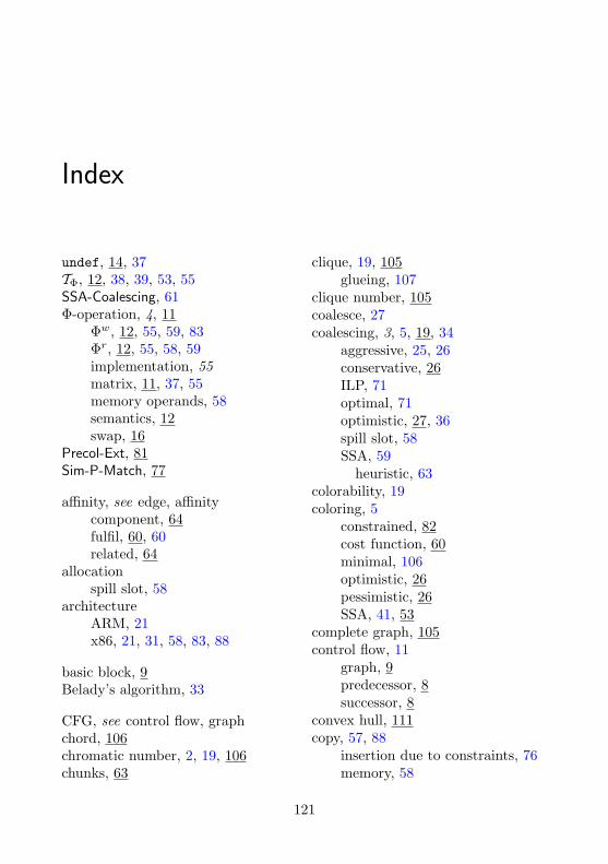
Index
undef, 14, 37TΦ, 12, 38, 39, 53, 55SSA-Coalescing, 61Φ-operation, 4, 11
Φw, 12, 55, 59, 83Φr, 12, 55, 58, 59implementation, 55matrix, 11, 37, 55memory operands, 58semantics, 12swap, 16
Precol-Ext, 81Sim-P-Match, 77
affinity, see edge, affinitycomponent, 64fulfil, 60, 60related, 64
allocationspill slot, 58
architectureARM, 21x86, 21, 31, 58, 83, 88
basic block, 9Belady’s algorithm, 33
CFG, see control flow, graphchord, 106chromatic number, 2, 19, 106chunks, 63
clique, 19, 105glueing, 107
clique number, 105coalesce, 27coalescing, 3, 5, 19, 34
aggressive, 25, 26conservative, 26ILP, 71optimal, 71optimistic, 27, 36spill slot, 58SSA, 59
heuristic, 63colorability, 19coloring, 5
constrained, 82cost function, 60minimal, 106optimistic, 26pessimistic, 26SSA, 41, 53
complete graph, 105control flow, 11
graph, 9predecessor, 8successor, 8
convex hull, 111copy, 57, 88
insertion due to constraints, 76memory, 58
121

122 Index
cut, 112cuts
clique-ray, 74path, 73
cycle, 40, 105
def-use chains, 68definition, 9degree
significant, 27dominance, 10, 68
immediate, 10tree order, 10, 39
edgeaffinity, 19, 59critical, 10
executionfrequencies, 59
feasible region, 111feasible solution, 111Firm, 87freeze, 27
graph1-perfect, 30bipartite, 77, 106chordal, 4, 5, 31, 39, 107chromatic number, 5coloring, 2interference
uncolorable, 75perfect, 5, 30, 106rigid-circuit, 107triangulated, 107
IG, see graph, interferenceinduced subgraph, 105integer linear programming, 34, 59,
111
interference, 2, 17, 18graph, 2, 17, 21
chordal, 40precoloring, 81SSA, 40SSA vs. non-SSA, 40storage, 33
neighbors, 69test, 68
Just-In-Time compilation, 33just-in-time compilation, 3
label, see program, labellinear scan, 34linearly ordered set, 7list, 7live range, 17
splitting, 18, 19, 26, 28, 34, 36,82, 88
liveness, 1, 17, 68and Φ-operations, 37SSA, 38
lost copies, 15
matching, 106C-perfect, 77perfect, 106
maximum cardinality search, 30
orientation, 108R, 39, 108
parallel copy, 40, 60path, 9, 105PEO, see perfect elimination orderperfect elimination order, 108processors, 21program, 8
label, 8strict, 10, 18, 39
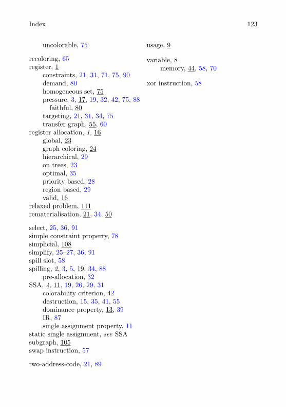
Index 123
uncolorable, 75
recoloring, 65register, 1
constraints, 21, 31, 71, 75, 90demand, 80homogeneous set, 75pressure, 3, 17, 19, 32, 42, 75, 88
faithful, 80targeting, 21, 31, 34, 75transfer graph, 55, 60
register allocation, 1, 16global, 23graph coloring, 24hierarchical, 29on trees, 23optimal, 35priority based, 28region based, 29valid, 16
relaxed problem, 111rematerialisation, 21, 34, 50
select, 25, 36, 91simple constraint property, 78simplicial, 108simplify, 25–27, 36, 91spill slot, 58spilling, 2, 3, 5, 19, 34, 88
pre-allocation, 32SSA, 4, 11, 19, 26, 29, 31
colorability criterion, 42destruction, 15, 35, 41, 55dominance property, 13, 39IR, 87single assignment property, 11
static single assignment, see SSAsubgraph, 105swap instruction, 57
two-address-code, 21, 89
usage, 9
variable, 8memory, 44, 58, 70
xor instruction, 58