regress — Linear regression · vce(hc3) produces conﬁdence intervals that tend to be even more conservative. See Davidson and MacKinnon (1993, 554–556) and Angrist and Pischke

Title

regress — Linear regression

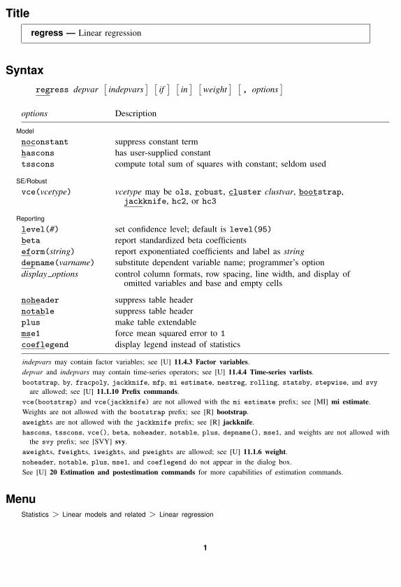
Syntaxregress depvar

[indepvars

] [if] [

in] [

weight] [

, options]

options Description

Model

noconstant suppress constant termhascons has user-supplied constanttsscons compute total sum of squares with constant; seldom used

SE/Robust

vce(vcetype) vcetype may be ols, robust, cluster clustvar, bootstrap,jackknife, hc2, or hc3

Reporting

level(#) set confidence level; default is level(95)

beta report standardized beta coefficientseform(string) report exponentiated coefficients and label as stringdepname(varname) substitute dependent variable name; programmer’s optiondisplay options control column formats, row spacing, line width, and display of

omitted variables and base and empty cells

noheader suppress table headernotable suppress table headerplus make table extendablemse1 force mean squared error to 1

coeflegend display legend instead of statistics

indepvars may contain factor variables; see [U] 11.4.3 Factor variables.depvar and indepvars may contain time-series operators; see [U] 11.4.4 Time-series varlists.bootstrap, by, fracpoly, jackknife, mfp, mi estimate, nestreg, rolling, statsby, stepwise, and svy

are allowed; see [U] 11.1.10 Prefix commands.vce(bootstrap) and vce(jackknife) are not allowed with the mi estimate prefix; see [MI] mi estimate.Weights are not allowed with the bootstrap prefix; see [R] bootstrap.aweights are not allowed with the jackknife prefix; see [R] jackknife.hascons, tsscons, vce(), beta, noheader, notable, plus, depname(), mse1, and weights are not allowed with

the svy prefix; see [SVY] svy.aweights, fweights, iweights, and pweights are allowed; see [U] 11.1.6 weight.noheader, notable, plus, mse1, and coeflegend do not appear in the dialog box.See [U] 20 Estimation and postestimation commands for more capabilities of estimation commands.

MenuStatistics > Linear models and related > Linear regression

1

2 regress — Linear regression

Descriptionregress fits a model of depvar on indepvars using linear regression.

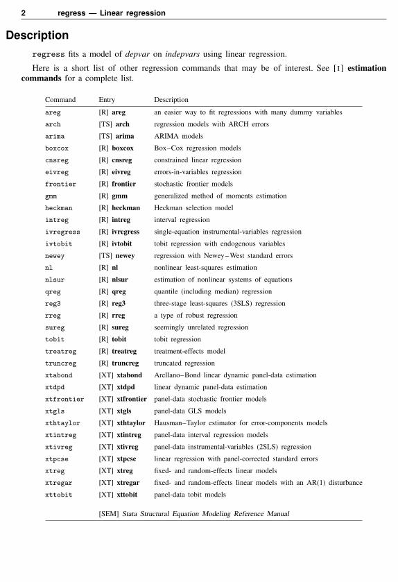
Here is a short list of other regression commands that may be of interest. See [ I ] estimationcommands for a complete list.

Command Entry Description

areg [R] areg an easier way to fit regressions with many dummy variables

arch [TS] arch regression models with ARCH errors

arima [TS] arima ARIMA models

boxcox [R] boxcox Box–Cox regression models

cnsreg [R] cnsreg constrained linear regression

eivreg [R] eivreg errors-in-variables regression

frontier [R] frontier stochastic frontier models

gmm [R] gmm generalized method of moments estimation

heckman [R] heckman Heckman selection model

intreg [R] intreg interval regression

ivregress [R] ivregress single-equation instrumental-variables regression

ivtobit [R] ivtobit tobit regression with endogenous variables

newey [TS] newey regression with Newey–West standard errors

nl [R] nl nonlinear least-squares estimation

nlsur [R] nlsur estimation of nonlinear systems of equations

qreg [R] qreg quantile (including median) regression

reg3 [R] reg3 three-stage least-squares (3SLS) regression

rreg [R] rreg a type of robust regression

sureg [R] sureg seemingly unrelated regression

tobit [R] tobit tobit regression

treatreg [R] treatreg treatment-effects model

truncreg [R] truncreg truncated regression

xtabond [XT] xtabond Arellano–Bond linear dynamic panel-data estimation

xtdpd [XT] xtdpd linear dynamic panel-data estimation

xtfrontier [XT] xtfrontier panel-data stochastic frontier models

xtgls [XT] xtgls panel-data GLS models

xthtaylor [XT] xthtaylor Hausman–Taylor estimator for error-components models

xtintreg [XT] xtintreg panel-data interval regression models

xtivreg [XT] xtivreg panel-data instrumental-variables (2SLS) regression

xtpcse [XT] xtpcse linear regression with panel-corrected standard errors

xtreg [XT] xtreg fixed- and random-effects linear models

xtregar [XT] xtregar fixed- and random-effects linear models with an AR(1) disturbance

xttobit [XT] xttobit panel-data tobit models

[SEM] Stata Structural Equation Modeling Reference Manual

regress — Linear regression 3

Options

� � �Model �

noconstant; see [R] estimation options.

hascons indicates that a user-defined constant or its equivalent is specified among the independentvariables in indepvars. Some caution is recommended when specifying this option, as resultingestimates may not be as accurate as they otherwise would be. Use of this option requires “sweeping”the constant last, so the moment matrix must be accumulated in absolute rather than deviation form.This option may be safely specified when the means of the dependent and independent variablesare all reasonable and there is not much collinearity between the independent variables. The bestprocedure is to view hascons as a reporting option—estimate with and without hascons andverify that the coefficients and standard errors of the variables not affected by the identity of theconstant are unchanged.

tsscons forces the total sum of squares to be computed as though the model has a constant, that is,as deviations from the mean of the dependent variable. This is a rarely used option that has aneffect only when specified with noconstant. It affects the total sum of squares and all resultsderived from the total sum of squares.

� � �SE/Robust �

vce(vcetype) specifies the type of standard error reported, which includes types that are derivedfrom asymptotic theory, that are robust to some kinds of misspecification, that allow for intragroupcorrelation, and that use bootstrap or jackknife methods; see [R] vce option.

vce(ols), the default, uses the standard variance estimator for ordinary least-squares regression.

regress also allows the following:

vce(hc2) and vce(hc3) specify an alternative bias correction for the robust variance calculation.vce(hc2) and vce(hc3) may not be specified with svy prefix. In the unclustered case,vce(robust) uses σ2

j = {n/(n−k)}u2j as an estimate of the variance of the jth observation,

where uj is the calculated residual and n/(n− k) is included to improve the overall estimate’ssmall-sample properties.

vce(hc2) instead uses u2j/(1 − hjj) as the observation’s variance estimate, where hjj is

the diagonal element of the hat (projection) matrix. This estimate is unbiased if the modelreally is homoskedastic. vce(hc2) tends to produce slightly more conservative confidenceintervals.

vce(hc3) uses u2j/(1−hjj)2 as suggested by Davidson and MacKinnon (1993), who report

that this method tends to produce better results when the model really is heteroskedastic.vce(hc3) produces confidence intervals that tend to be even more conservative.

See Davidson and MacKinnon (1993, 554–556) and Angrist and Pischke (2009, 294–308)for more discussion on these two bias corrections.

� � �Reporting �

level(#); see [R] estimation options.

beta asks that standardized beta coefficients be reported instead of confidence intervals. The betacoefficients are the regression coefficients obtained by first standardizing all variables to have amean of 0 and a standard deviation of 1. beta may not be specified with vce(cluster clustvar)or the svy prefix.


eform(string) is used only in programs and ado-files that use regress to fit models other thanlinear regression. eform() specifies that the coefficient table be displayed in exponentiated formas defined in [R] maximize and that string be used to label the exponentiated coefficients in thetable.

depname(varname) is used only in programs and ado-files that use regress to fit models other thanlinear regression. depname() may be specified only at estimation time. varname is recorded asthe identity of the dependent variable, even though the estimates are calculated using depvar. Thismethod affects the labeling of the output—not the results calculated—but could affect subsequentcalculations made by predict, where the residual would be calculated as deviations from varnamerather than depvar. depname() is most typically used when depvar is a temporary variable (see[P] macro) used as a proxy for varname.

depname() is not allowed with the svy prefix.

display options: noomitted, vsquish, noemptycells, baselevels, allbaselevels,cformat(% fmt), pformat(% fmt), sformat(% fmt), and nolstretch; see [R] estimation options.

The following options are available with regress but are not shown in the dialog box:

noheader suppresses the display of the ANOVA table and summary statistics at the top of the output;only the coefficient table is displayed. This option is often used in programs and ado-files.

notable suppresses display of the coefficient table.

plus specifies that the output table be made extendable. This option is often used in programs andado-files.

mse1 is used only in programs and ado-files that use regress to fit models other than linearregression and is not allowed with the svy prefix. mse1 sets the mean squared error to 1, forcingthe variance–covariance matrix of the estimators to be (X′DX)−1 (see Methods and formulasbelow) and affecting calculated standard errors. Degrees of freedom for t statistics are calculatedas n rather than n− k.

coeflegend; see [R] estimation options.

RemarksRemarks are presented under the following headings:

Ordinary least squaresTreatment of the constantRobust standard errorsWeighted regressionInstrumental variables and two-stage least-squares regression

regress performs linear regression, including ordinary least squares and weighted least squares.For a general discussion of linear regression, see Draper and Smith (1998), Greene (2012), orKmenta (1997).

See Wooldridge (2009) for an excellent treatment of estimation, inference, interpretation, andspecification testing in linear regression models. This presentation stands out for its clarification ofthe statistical issues, as opposed to the algebraic issues. See Wooldridge (2010, chap. 4) for a moreadvanced discussion along the same lines.

See Hamilton (2009, chap. 6) and Cameron and Trivedi (2010, chap. 3) for an introductionto linear regression using Stata. Dohoo, Martin, and Stryhn (2010) discuss linear regression usingexamples from epidemiology, and Stata datasets and do-files used in the text are available. Cameronand Trivedi (2010) discuss linear regression using econometric examples with Stata.


Chatterjee and Hadi (2006) explain regression analysis by using examples containing typicalproblems that you might encounter when performing exploratory data analysis. We also recommendWeisberg (2005), who emphasizes the importance of the assumptions of linear regression andproblems resulting from these assumptions. Angrist and Pischke (2009) approach regression as atool for exploring relationships, estimating treatment effects, and providing answers to public policyquestions. For a discussion of model-selection techniques and exploratory data analysis, see Mostellerand Tukey (1977). For a mathematically rigorous treatment, see Peracchi (2001, chap. 6). Finally,see Plackett (1972) if you are interested in the history of regression. Least squares, which dates backto the 1790s, was discovered independently by Legendre and Gauss.

Ordinary least squares

Example 1

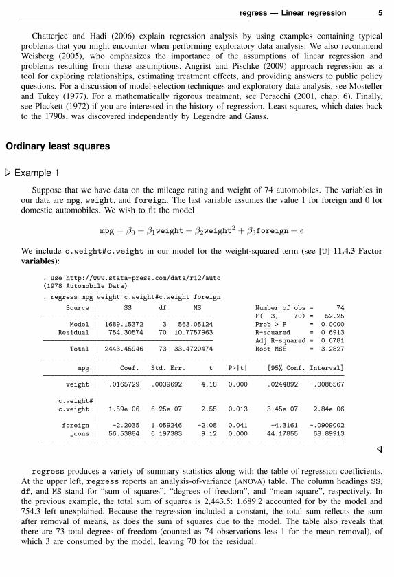
Suppose that we have data on the mileage rating and weight of 74 automobiles. The variables inour data are mpg, weight, and foreign. The last variable assumes the value 1 for foreign and 0 fordomestic automobiles. We wish to fit the model

mpg = β0 + β1weight + β2weight2 + β3foreign + ε

We include c.weight#c.weight in our model for the weight-squared term (see [U] 11.4.3 Factorvariables):

. use http://www.stata-press.com/data/r12/auto(1978 Automobile Data)

. regress mpg weight c.weight#c.weight foreign

Source SS df MS Number of obs = 74F( 3, 70) = 52.25

Model 1689.15372 3 563.05124 Prob > F = 0.0000Residual 754.30574 70 10.7757963 R-squared = 0.6913

Adj R-squared = 0.6781Total 2443.45946 73 33.4720474 Root MSE = 3.2827

mpg Coef. Std. Err. t P>|t| [95% Conf. Interval]

weight -.0165729 .0039692 -4.18 0.000 -.0244892 -.0086567

c.weight#c.weight 1.59e-06 6.25e-07 2.55 0.013 3.45e-07 2.84e-06

foreign -2.2035 1.059246 -2.08 0.041 -4.3161 -.0909002_cons 56.53884 6.197383 9.12 0.000 44.17855 68.89913

regress produces a variety of summary statistics along with the table of regression coefficients.At the upper left, regress reports an analysis-of-variance (ANOVA) table. The column headings SS,df, and MS stand for “sum of squares”, “degrees of freedom”, and “mean square”, respectively. Inthe previous example, the total sum of squares is 2,443.5: 1,689.2 accounted for by the model and754.3 left unexplained. Because the regression included a constant, the total sum reflects the sumafter removal of means, as does the sum of squares due to the model. The table also reveals thatthere are 73 total degrees of freedom (counted as 74 observations less 1 for the mean removal), ofwhich 3 are consumed by the model, leaving 70 for the residual.


To the right of the ANOVA table are presented other summary statistics. The F statistic associatedwith the ANOVA table is 52.25. The statistic has 3 numerator and 70 denominator degrees of freedom.The F statistic tests the hypothesis that all coefficients excluding the constant are zero. The chance ofobserving an F statistic that large or larger is reported as 0.0000, which is Stata’s way of indicatinga number smaller than 0.00005. The R-squared (R2) for the regression is 0.6913, and the R-squaredadjusted for degrees of freedom (R2

a) is 0.6781. The root mean squared error, labeled Root MSE, is3.2827. It is the square root of the mean squared error reported for the residual in the ANOVA table.

Finally, Stata produces a table of the estimated coefficients. The first line of the table indicatesthat the left-hand-side variable is mpg. Thereafter follow the four estimated coefficients. Our fittedmodel is

mpg hat = 56.54− 0.0166 weight + 1.59× 10−6 c.weight#c.weight− 2.20 foreign

Reported to the right of the coefficients in the output are the standard errors. For instance, thestandard error for the coefficient on weight is 0.0039692. The corresponding t statistic is −4.18,which has a two-sided significance level of 0.000. This number indicates that the significance is lessthan 0.0005. The 95% confidence interval for the coefficient is [−0.024,−0.009 ].

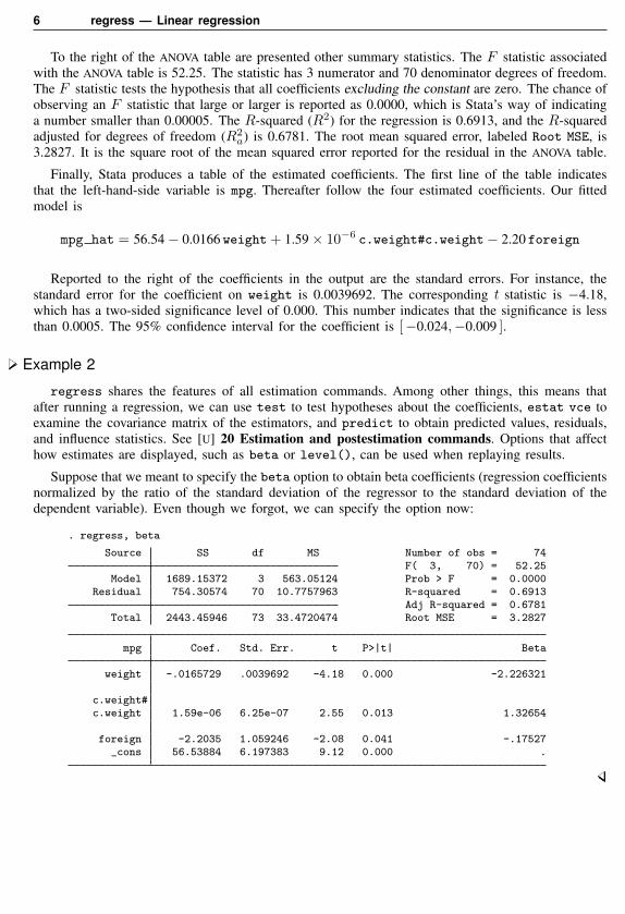
Example 2

regress shares the features of all estimation commands. Among other things, this means thatafter running a regression, we can use test to test hypotheses about the coefficients, estat vce toexamine the covariance matrix of the estimators, and predict to obtain predicted values, residuals,and influence statistics. See [U] 20 Estimation and postestimation commands. Options that affecthow estimates are displayed, such as beta or level(), can be used when replaying results.

Suppose that we meant to specify the beta option to obtain beta coefficients (regression coefficientsnormalized by the ratio of the standard deviation of the regressor to the standard deviation of thedependent variable). Even though we forgot, we can specify the option now:

. regress, beta




mpg Coef. Std. Err. t P>|t| Beta

weight -.0165729 .0039692 -4.18 0.000 -2.226321

c.weight#c.weight 1.59e-06 6.25e-07 2.55 0.013 1.32654

foreign -2.2035 1.059246 -2.08 0.041 -.17527_cons 56.53884 6.197383 9.12 0.000 .


Treatment of the constantBy default, regress includes an intercept (constant) term in the model. The noconstant option

suppresses it, and the hascons option tells regress that the model already has one.

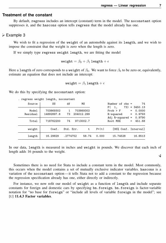
Example 3

We wish to fit a regression of the weight of an automobile against its length, and we wish toimpose the constraint that the weight is zero when the length is zero.

If we simply type regress weight length, we are fitting the model

weight = β0 + β1 length + ε

Here a length of zero corresponds to a weight of β0. We want to force β0 to be zero or, equivalently,estimate an equation that does not include an intercept:

weight = β1 length + ε

We do this by specifying the noconstant option:

. regress weight length, noconstant


Model 703869302 1 703869302 Prob > F = 0.0000Residual 14892897.8 73 204012.299 R-squared = 0.9793

Adj R-squared = 0.9790Total 718762200 74 9713002.7 Root MSE = 451.68

weight Coef. Std. Err. t P>|t| [95% Conf. Interval]

length 16.29829 .2774752 58.74 0.000 15.74528 16.8513

In our data, length is measured in inches and weight in pounds. We discover that each inch oflength adds 16 pounds to the weight.

Sometimes there is no need for Stata to include a constant term in the model. Most commonly,this occurs when the model contains a set of mutually exclusive indicator variables. hascons is avariation of the noconstant option—it tells Stata not to add a constant to the regression becausethe regression specification already has one, either directly or indirectly.

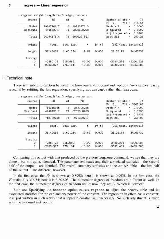
For instance, we now refit our model of weight as a function of length and include separateconstants for foreign and domestic cars by specifying bn.foreign. bn.foreign is factor-variablenotation for “no base for foreign” or “include all levels of variable foreign in the model”; see[U] 11.4.3 Factor variables.


. regress weight length bn.foreign, hascons





length 31.44455 1.601234 19.64 0.000 28.25178 34.63732

foreign0 -2850.25 315.9691 -9.02 0.000 -3480.274 -2220.2251 -2983.927 275.1041 -10.85 0.000 -3532.469 -2435.385

Technical note

There is a subtle distinction between the hascons and noconstant options. We can most easilyreveal it by refitting the last regression, specifying noconstant rather than hascons:

. regress weight length bn.foreign, noconstant


Model 714315766 3 238105255 Prob > F = 0.0000Residual 4446433.7 71 62625.8268 R-squared = 0.9938

Adj R-squared = 0.9936Total 718762200 74 9713002.7 Root MSE = 250.25


length 31.44455 1.601234 19.64 0.000 28.25178 34.63732

foreign0 -2850.25 315.9691 -9.02 0.000 -3480.274 -2220.2251 -2983.927 275.1041 -10.85 0.000 -3532.469 -2435.385

Comparing this output with that produced by the previous regress command, we see that they arealmost, but not quite, identical. The parameter estimates and their associated statistics—the secondhalf of the output—are identical. The overall summary statistics and the ANOVA table—the first halfof the output—are different, however.

In the first case, the R2 is shown as 0.8992; here it is shown as 0.9938. In the first case, theF statistic is 316.54; now it is 3,802.03. The numerator degrees of freedom are different as well. Inthe first case, the numerator degrees of freedom are 2; now they are 3. Which is correct?

Both are. Specifying the hascons option causes regress to adjust the ANOVA table and itsassociated statistics for the explanatory power of the constant. The regression in effect has a constant;it is just written in such a way that a separate constant is unnecessary. No such adjustment is madewith the noconstant option.


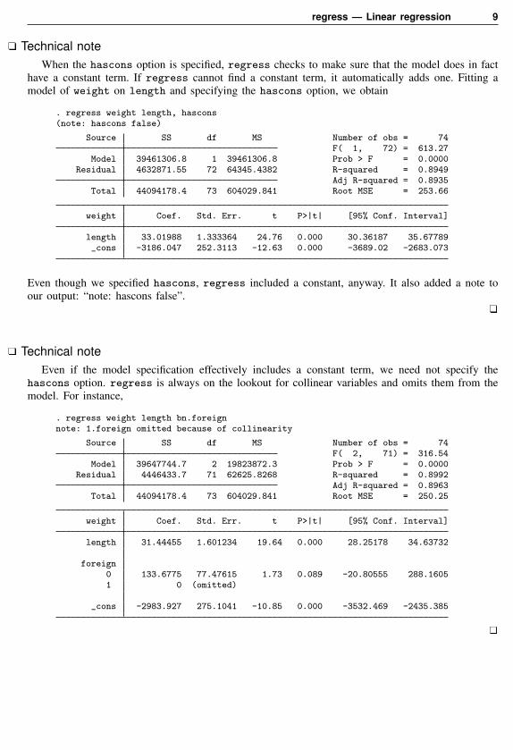
Technical noteWhen the hascons option is specified, regress checks to make sure that the model does in fact

have a constant term. If regress cannot find a constant term, it automatically adds one. Fitting amodel of weight on length and specifying the hascons option, we obtain

. regress weight length, hascons(note: hascons false)





length 33.01988 1.333364 24.76 0.000 30.36187 35.67789_cons -3186.047 252.3113 -12.63 0.000 -3689.02 -2683.073

Even though we specified hascons, regress included a constant, anyway. It also added a note toour output: “note: hascons false”.

Technical noteEven if the model specification effectively includes a constant term, we need not specify the

hascons option. regress is always on the lookout for collinear variables and omits them from themodel. For instance,

. regress weight length bn.foreignnote: 1.foreign omitted because of collinearity





length 31.44455 1.601234 19.64 0.000 28.25178 34.63732

foreign0 133.6775 77.47615 1.73 0.089 -20.80555 288.16051 0 (omitted)

_cons -2983.927 275.1041 -10.85 0.000 -3532.469 -2435.385


Robust standard errorsregress with the vce(robust) option substitutes a robust variance matrix calculation for the

conventional calculation, or if vce(cluster clustvar) is specified, allows relaxing the assumptionof independence within groups. How this method works is explained in [U] 20.20 Obtaining robustvariance estimates. Below we show how well this approach works.

Example 4

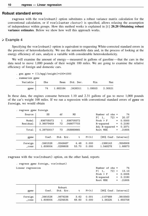
Specifying the vce(robust) option is equivalent to requesting White-corrected standard errors inthe presence of heteroskedasticity. We use the automobile data and, in the process of looking at theenergy efficiency of cars, analyze a variable with considerable heteroskedasticity.

We will examine the amount of energy—measured in gallons of gasoline—that the cars in thedata need to move 1,000 pounds of their weight 100 miles. We are going to examine the relativeefficiency of foreign and domestic cars.

. gen gpmw = ((1/mpg)/weight)*100*1000

. summarize gpmw

Variable Obs Mean Std. Dev. Min Max

gpmw 74 1.682184 .2426311 1.09553 2.30521

In these data, the engines consume between 1.10 and 2.31 gallons of gas to move 1,000 poundsof the car’s weight 100 miles. If we ran a regression with conventional standard errors of gpmw onforeign, we would obtain

. regress gpmw foreign


Model .936705572 1 .936705572 Prob > F = 0.0000Residual 3.36079459 72 .046677703 R-squared = 0.2180

Adj R-squared = 0.2071Total 4.29750017 73 .058869865 Root MSE = .21605

gpmw Coef. Std. Err. t P>|t| [95% Conf. Interval]

foreign .2461526 .0549487 4.48 0.000 .1366143 .3556909_cons 1.609004 .0299608 53.70 0.000 1.549278 1.66873

regress with the vce(robust) option, on the other hand, reports

. regress gpmw foreign, vce(robust)

Linear regression Number of obs = 74F( 1, 72) = 13.13Prob > F = 0.0005R-squared = 0.2180Root MSE = .21605

Robustgpmw Coef. Std. Err. t P>|t| [95% Conf. Interval]

foreign .2461526 .0679238 3.62 0.001 .1107489 .3815563_cons 1.609004 .0234535 68.60 0.000 1.56225 1.655758


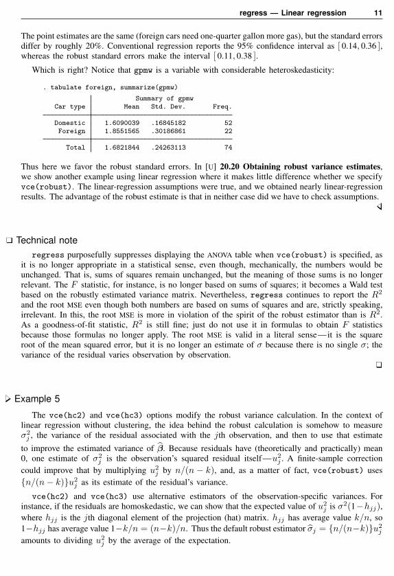
The point estimates are the same (foreign cars need one-quarter gallon more gas), but the standard errorsdiffer by roughly 20%. Conventional regression reports the 95% confidence interval as [ 0.14, 0.36 ],whereas the robust standard errors make the interval [ 0.11, 0.38 ].

Which is right? Notice that gpmw is a variable with considerable heteroskedasticity:

. tabulate foreign, summarize(gpmw)

Summary of gpmwCar type Mean Std. Dev. Freq.

Domestic 1.6090039 .16845182 52Foreign 1.8551565 .30186861 22

Total 1.6821844 .24263113 74

Thus here we favor the robust standard errors. In [U] 20.20 Obtaining robust variance estimates,we show another example using linear regression where it makes little difference whether we specifyvce(robust). The linear-regression assumptions were true, and we obtained nearly linear-regressionresults. The advantage of the robust estimate is that in neither case did we have to check assumptions.

Technical noteregress purposefully suppresses displaying the ANOVA table when vce(robust) is specified, as

it is no longer appropriate in a statistical sense, even though, mechanically, the numbers would beunchanged. That is, sums of squares remain unchanged, but the meaning of those sums is no longerrelevant. The F statistic, for instance, is no longer based on sums of squares; it becomes a Wald testbased on the robustly estimated variance matrix. Nevertheless, regress continues to report the R2

and the root MSE even though both numbers are based on sums of squares and are, strictly speaking,irrelevant. In this, the root MSE is more in violation of the spirit of the robust estimator than is R2.As a goodness-of-fit statistic, R2 is still fine; just do not use it in formulas to obtain F statisticsbecause those formulas no longer apply. The root MSE is valid in a literal sense—it is the squareroot of the mean squared error, but it is no longer an estimate of σ because there is no single σ; thevariance of the residual varies observation by observation.

Example 5

The vce(hc2) and vce(hc3) options modify the robust variance calculation. In the context oflinear regression without clustering, the idea behind the robust calculation is somehow to measureσ2

j , the variance of the residual associated with the jth observation, and then to use that estimate

to improve the estimated variance of β. Because residuals have (theoretically and practically) mean0, one estimate of σ2

j is the observation’s squared residual itself—u2j . A finite-sample correction

could improve that by multiplying u2j by n/(n − k), and, as a matter of fact, vce(robust) uses

{n/(n− k)}u2j as its estimate of the residual’s variance.

vce(hc2) and vce(hc3) use alternative estimators of the observation-specific variances. Forinstance, if the residuals are homoskedastic, we can show that the expected value of u2

j is σ2(1−hjj),where hjj is the jth diagonal element of the projection (hat) matrix. hjj has average value k/n, so1−hjj has average value 1−k/n = (n−k)/n. Thus the default robust estimator σj = {n/(n−k)}u2

j

amounts to dividing u2j by the average of the expectation.


vce(hc2) divides u2j by 1−hjj itself, so it should yield better estimates if the residuals really are

homoskedastic. vce(hc3) divides u2j by (1− hjj)2 and has no such clean interpretation. Davidson

and MacKinnon (1993) show that u2j/(1 − hjj)2 approximates a more complicated estimator that

they obtain by jackknifing (MacKinnon and White 1985). Angrist and Pischke (2009) also illustratethe relative merits of these adjustments.

Here are the results of refitting our efficiency model using vce(hc2) and vce(hc3):

. regress gpmw foreign, vce(hc2)


Robust HC2gpmw Coef. Std. Err. t P>|t| [95% Conf. Interval]

foreign .2461526 .0684669 3.60 0.001 .1096662 .3826389_cons 1.609004 .0233601 68.88 0.000 1.562437 1.655571

. regress gpmw foreign, vce(hc3)


Robust HC3gpmw Coef. Std. Err. t P>|t| [95% Conf. Interval]

foreign .2461526 .069969 3.52 0.001 .1066719 .3856332_cons 1.609004 .023588 68.21 0.000 1.561982 1.656026

Example 6

The vce(cluster clustvar) option relaxes the assumption of independence. Below we have 28,534observations on 4,711 women aged 14–46 years. Data were collected on these women between 1968and 1988. We are going to fit a classic earnings model, and we begin by ignoring that each womanappears an average of 6.056 times in the data.


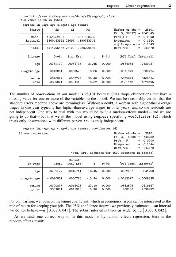
. use http://www.stata-press.com/data/r12/regsmpl, clear(NLS Women 14-26 in 1968)

. regress ln_wage age c.age#c.age tenure


Model 1054.52501 3 351.508335 Prob > F = 0.0000Residual 5360.43962 28097 .190783344 R-squared = 0.1644

Adj R-squared = 0.1643Total 6414.96462 28100 .228290556 Root MSE = .43679

ln_wage Coef. Std. Err. t P>|t| [95% Conf. Interval]

age .0752172 .0034736 21.65 0.000 .0684088 .0820257

c.age#c.age -.0010851 .0000575 -18.86 0.000 -.0011979 -.0009724

tenure .0390877 .0007743 50.48 0.000 .0375699 .0406054_cons .3339821 .0504413 6.62 0.000 .2351148 .4328495

The number of observations in our model is 28,101 because Stata drops observations that have amissing value for one or more of the variables in the model. We can be reasonably certain that thestandard errors reported above are meaningless. Without a doubt, a woman with higher-than-averagewages in one year typically has higher-than-average wages in other years, and so the residuals arenot independent. One way to deal with this would be to fit a random-effects model—and we aregoing to do that—but first we fit the model using regress specifying vce(cluster id), whichtreats only observations with different person ids as truly independent:

. regress ln_wage age c.age#c.age tenure, vce(cluster id)


(Std. Err. adjusted for 4699 clusters in idcode)

Robustln_wage Coef. Std. Err. t P>|t| [95% Conf. Interval]

age .0752172 .0045711 16.45 0.000 .0662557 .0841788

c.age#c.age -.0010851 .0000778 -13.94 0.000 -.0012377 -.0009325

tenure .0390877 .0014425 27.10 0.000 .0362596 .0419157_cons .3339821 .0641918 5.20 0.000 .208136 .4598282

For comparison, we focus on the tenure coefficient, which in economics jargon can be interpreted as therate of return for keeping your job. The 95% confidence interval we previously estimated—an intervalwe do not believe—is [ 0.038, 0.041 ]. The robust interval is twice as wide, being [ 0.036, 0.042 ].

As we said, one correct way to fit this model is by random-effects regression. Here is therandom-effects result:


. xtreg ln_wage age c.age#c.age tenure, re

Random-effects GLS regression Number of obs = 28101Group variable: idcode Number of groups = 4699

R-sq: within = 0.1370 Obs per group: min = 1between = 0.2154 avg = 6.0overall = 0.1608 max = 15

Random effects u_i ~ Gaussian Wald chi2(3) = 4717.05corr(u_i, X) = 0 (assumed) Prob > chi2 = 0.0000

ln_wage Coef. Std. Err. z P>|z| [95% Conf. Interval]

age .0568296 .0026958 21.08 0.000 .0515459 .0621132

c.age#c.age -.0007566 .0000447 -16.93 0.000 -.0008441 -.000669

tenure .0260135 .0007477 34.79 0.000 .0245481 .0274789_cons .6136792 .0394611 15.55 0.000 .5363368 .6910216

sigma_u .33542449sigma_e .29674679

rho .56095413 (fraction of variance due to u_i)

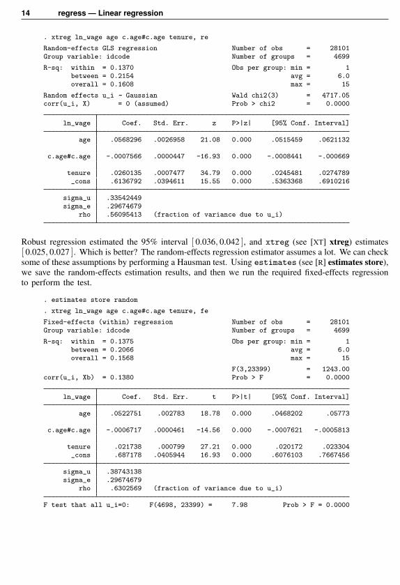
Robust regression estimated the 95% interval [ 0.036, 0.042 ], and xtreg (see [XT] xtreg) estimates[ 0.025, 0.027 ]. Which is better? The random-effects regression estimator assumes a lot. We can checksome of these assumptions by performing a Hausman test. Using estimates (see [R] estimates store),we save the random-effects estimation results, and then we run the required fixed-effects regressionto perform the test.

. estimates store random

. xtreg ln_wage age c.age#c.age tenure, fe

Fixed-effects (within) regression Number of obs = 28101Group variable: idcode Number of groups = 4699

R-sq: within = 0.1375 Obs per group: min = 1between = 0.2066 avg = 6.0overall = 0.1568 max = 15

F(3,23399) = 1243.00corr(u_i, Xb) = 0.1380 Prob > F = 0.0000

ln_wage Coef. Std. Err. t P>|t| [95% Conf. Interval]

age .0522751 .002783 18.78 0.000 .0468202 .05773

c.age#c.age -.0006717 .0000461 -14.56 0.000 -.0007621 -.0005813

tenure .021738 .000799 27.21 0.000 .020172 .023304_cons .687178 .0405944 16.93 0.000 .6076103 .7667456

sigma_u .38743138sigma_e .29674679

rho .6302569 (fraction of variance due to u_i)

F test that all u_i=0: F(4698, 23399) = 7.98 Prob > F = 0.0000


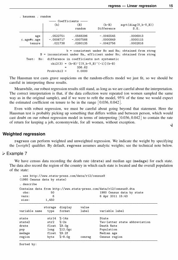
. hausman . random

Coefficients(b) (B) (b-B) sqrt(diag(V_b-V_B)). random Difference S.E.

age .0522751 .0568296 -.0045545 .0006913c.age#c.age -.0006717 -.0007566 .0000849 .0000115

tenure .021738 .0260135 -.0042756 .0002816

b = consistent under Ho and Ha; obtained from xtregB = inconsistent under Ha, efficient under Ho; obtained from xtreg

Test: Ho: difference in coefficients not systematic

chi2(3) = (b-B)’[(V_b-V_B)^(-1)](b-B)= 336.62

Prob>chi2 = 0.0000

The Hausman test casts grave suspicions on the random-effects model we just fit, so we should becareful in interpreting those results.

Meanwhile, our robust regression results still stand, as long as we are careful about the interpretation.The correct interpretation is that, if the data collection were repeated (on women sampled the sameway as in the original sample), and if we were to refit the model, 95% of the time we would expectthe estimated coefficient on tenure to be in the range [ 0.036, 0.042 ].

Even with robust regression, we must be careful about going beyond that statement. Here theHausman test is probably picking up something that differs within and between person, which wouldcast doubt on our robust regression model in terms of interpreting [ 0.036, 0.042 ] to contain the rateof return for keeping a job, economywide, for all women, without exception.

Weighted regressionregress can perform weighted and unweighted regression. We indicate the weight by specifying

the [weight] qualifier. By default, regress assumes analytic weights; see the technical note below.

Example 7

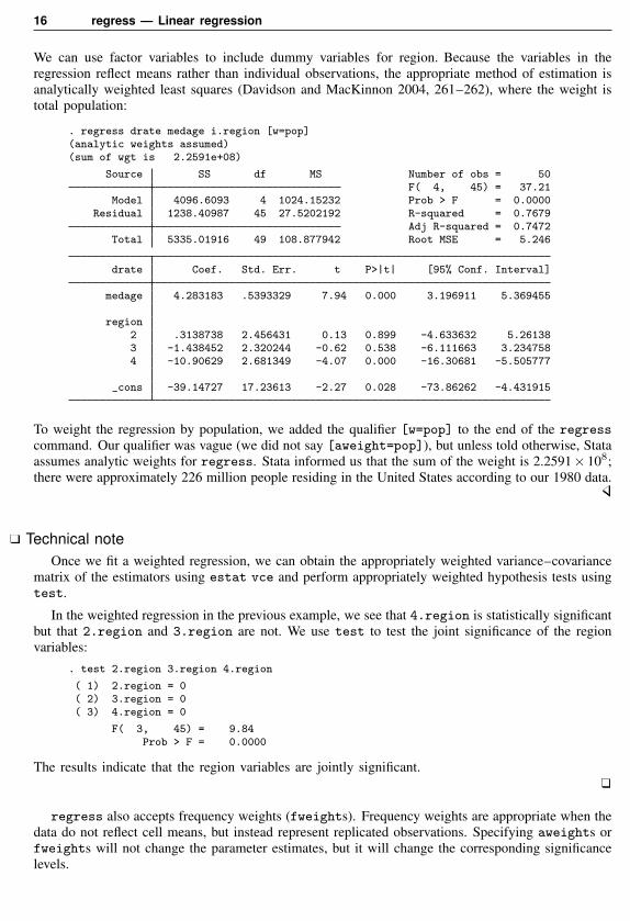
We have census data recording the death rate (drate) and median age (medage) for each state.The data also record the region of the country in which each state is located and the overall populationof the state:

. use http://www.stata-press.com/data/r12/census9(1980 Census data by state)

. describe

Contains data from http://www.stata-press.com/data/r12/census9.dtaobs: 50 1980 Census data by state

vars: 6 6 Apr 2011 15:43size: 1,450

storage display valuevariable name type format label variable label

state str14 %-14s Statestate2 str2 %-2s Two-letter state abbreviationdrate float %9.0g Death Ratepop long %12.0gc Populationmedage float %9.2f Median ageregion byte %-8.0g cenreg Census region

Sorted by:


We can use factor variables to include dummy variables for region. Because the variables in theregression reflect means rather than individual observations, the appropriate method of estimation isanalytically weighted least squares (Davidson and MacKinnon 2004, 261–262), where the weight istotal population:

. regress drate medage i.region [w=pop](analytic weights assumed)(sum of wgt is 2.2591e+08)




drate Coef. Std. Err. t P>|t| [95% Conf. Interval]

medage 4.283183 .5393329 7.94 0.000 3.196911 5.369455

region2 .3138738 2.456431 0.13 0.899 -4.633632 5.261383 -1.438452 2.320244 -0.62 0.538 -6.111663 3.2347584 -10.90629 2.681349 -4.07 0.000 -16.30681 -5.505777

_cons -39.14727 17.23613 -2.27 0.028 -73.86262 -4.431915

To weight the regression by population, we added the qualifier [w=pop] to the end of the regresscommand. Our qualifier was vague (we did not say [aweight=pop]), but unless told otherwise, Stataassumes analytic weights for regress. Stata informed us that the sum of the weight is 2.2591× 108;there were approximately 226 million people residing in the United States according to our 1980 data.

Technical noteOnce we fit a weighted regression, we can obtain the appropriately weighted variance–covariance

matrix of the estimators using estat vce and perform appropriately weighted hypothesis tests usingtest.

In the weighted regression in the previous example, we see that 4.region is statistically significantbut that 2.region and 3.region are not. We use test to test the joint significance of the regionvariables:

. test 2.region 3.region 4.region

( 1) 2.region = 0( 2) 3.region = 0( 3) 4.region = 0

F( 3, 45) = 9.84Prob > F = 0.0000

The results indicate that the region variables are jointly significant.

regress also accepts frequency weights (fweights). Frequency weights are appropriate when thedata do not reflect cell means, but instead represent replicated observations. Specifying aweights orfweights will not change the parameter estimates, but it will change the corresponding significancelevels.


For instance, if we specified [fweight=pop] in the weighted regression example above—whichwould be statistically incorrect—Stata would treat the data as if the data represented 226 millionindependent observations on death rates and median age. The data most certainly do not representthat—they represent 50 observations on state averages.

With aweights, Stata treats the number of observations on the process as the number of observationsin the data. When we specify fweights, Stata treats the number of observations as if it were equalto the sum of the weights; see Methods and formulas below.

Technical noteA popular request on the help line is to describe the effect of specifying [aweight=exp] with

regress in terms of transformation of the dependent and independent variables. The mechanicalanswer is that typing

. regress y x1 x2 [aweight=n]

is equivalent to fitting the model

yj√nj = β0

√nj + β1x1j

√nj + β2x2j

√nj + uj

√nj

This regression will reproduce the coefficients and covariance matrix produced by the aweightedregression. The mean squared errors (estimates of the variance of the residuals) will, however,be different. The transformed regression reports s2t , an estimate of Var(uj

√nj). The aweighted

regression reports s2a, an estimate of Var(uj√nj

√N/∑

k nk), whereN is the number of observations.Thus

s2a =N∑k nk

s2t =s2tn

(1)

The logic for this adjustment is as follows: Consider the model

y = β0 + β1x1 + β2x2 + u

Assume that, were this model fit on individuals, Var(u) = σ2u, a constant. Assume that individual

data are not available; what is available are averages (yj , x1j , x2j) for j = 1, . . . , N , and eachaverage is calculated over nj observations. Then it is still true that

yj = β0 + β1x1j + β2x2j + uj

where uj is the average of nj mean 0, variance σ2u deviates and has variance σ2

u = σ2u/nj . Thus

multiplying through by √nj produces

yj√nj = β0

√nj + β1x1j

√nj + β2x2j

√nj + uj

√nj

and Var(uj√nj) = σ2

u. The mean squared error, s2t , reported by fitting this transformed regressionis an estimate of σ2

u. The coefficients and covariance matrix could also be obtained by aweightedregress. The only difference would be in the reported mean squared error, which from (1) isσ2

u/n. On average, each observation in the data reflects the averages calculated over n =∑

k nk/Nindividuals, and thus this reported mean squared error is the average variance of an observation inthe dataset. We can retrieve the estimate of σ2

u by multiplying the reported mean squared error by n.

More generally, aweights are used to solve general heteroskedasticity problems. In these cases,we have the model

yj = β0 + β1x1j + β2x2j + uj


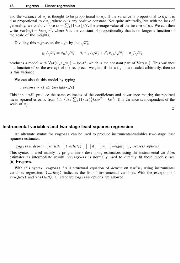
and the variance of uj is thought to be proportional to aj . If the variance is proportional to aj , it isalso proportional to αaj , where α is any positive constant. Not quite arbitrarily, but with no loss ofgenerality, we could choose α =

∑k(1/ak)/N , the average value of the inverse of aj . We can then

write Var(uj) = kαajσ2, where k is the constant of proportionality that is no longer a function of

the scale of the weights.

Dividing this regression through by the √aj ,

yj/√aj = β0/

√aj + β1x1j/

√aj + β2x2j/

√aj + uj/

√aj

produces a model with Var(uj/√aj) = kασ2, which is the constant part of Var(uj). This variance

is a function of α, the average of the reciprocal weights; if the weights are scaled arbitrarily, then sois this variance.

We can also fit this model by typing

. regress y x1 x2 [aweight=1/a]

This input will produce the same estimates of the coefficients and covariance matrix; the reportedmean squared error is, from (1),

{N/∑

k(1/ak)}kασ2 = kσ2. This variance is independent of the

scale of aj .

Instrumental variables and two-stage least-squares regression

An alternate syntax for regress can be used to produce instrumental-variables (two-stage leastsquares) estimates.

regress depvar[

varlist1[(varlist2)

] ] [if] [

in] [

weight] [

, regress options ]

This syntax is used mainly by programmers developing estimators using the instrumental-variablesestimates as intermediate results. ivregress is normally used to directly fit these models; see[R] ivregress.

With this syntax, regress fits a structural equation of depvar on varlist1 using instrumentalvariables regression; (varlist2) indicates the list of instrumental variables. With the exception ofvce(hc2) and vce(hc3), all standard regress options are allowed.


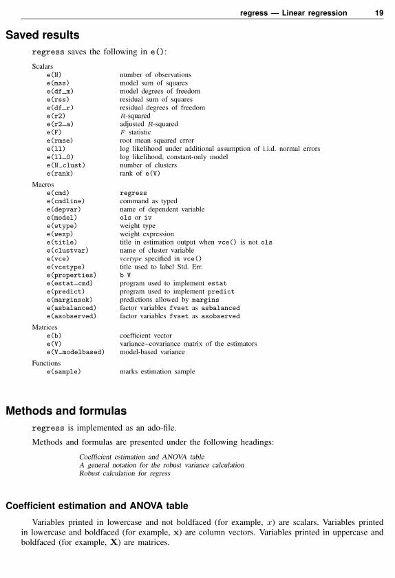
Saved resultsregress saves the following in e():

Scalarse(N) number of observationse(mss) model sum of squarese(df m) model degrees of freedome(rss) residual sum of squarese(df r) residual degrees of freedome(r2) R-squarede(r2 a) adjusted R-squarede(F) F statistice(rmse) root mean squared errore(ll) log likelihood under additional assumption of i.i.d. normal errorse(ll 0) log likelihood, constant-only modele(N clust) number of clusterse(rank) rank of e(V)

Macrose(cmd) regresse(cmdline) command as typede(depvar) name of dependent variablee(model) ols or ive(wtype) weight typee(wexp) weight expressione(title) title in estimation output when vce() is not olse(clustvar) name of cluster variablee(vce) vcetype specified in vce()e(vcetype) title used to label Std. Err.e(properties) b Ve(estat cmd) program used to implement estate(predict) program used to implement predicte(marginsok) predictions allowed by marginse(asbalanced) factor variables fvset as asbalancede(asobserved) factor variables fvset as asobserved

Matricese(b) coefficient vectore(V) variance–covariance matrix of the estimatorse(V modelbased) model-based variance

Functionse(sample) marks estimation sample

Methods and formulasregress is implemented as an ado-file.

Methods and formulas are presented under the following headings:

Coefficient estimation and ANOVA tableA general notation for the robust variance calculationRobust calculation for regress

Coefficient estimation and ANOVA table

Variables printed in lowercase and not boldfaced (for example, x) are scalars. Variables printedin lowercase and boldfaced (for example, x) are column vectors. Variables printed in uppercase andboldfaced (for example, X) are matrices.


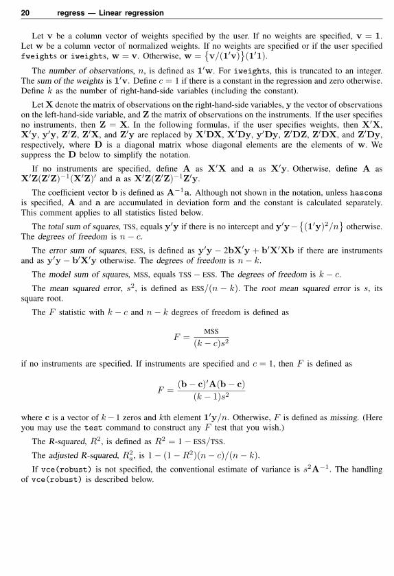
Let v be a column vector of weights specified by the user. If no weights are specified, v = 1.Let w be a column vector of normalized weights. If no weights are specified or if the user specifiedfweights or iweights, w = v. Otherwise, w =

{v/(1′v)

}(1′1).

The number of observations, n, is defined as 1′w. For iweights, this is truncated to an integer.The sum of the weights is 1′v. Define c = 1 if there is a constant in the regression and zero otherwise.Define k as the number of right-hand-side variables (including the constant).

Let X denote the matrix of observations on the right-hand-side variables, y the vector of observationson the left-hand-side variable, and Z the matrix of observations on the instruments. If the user specifiesno instruments, then Z = X. In the following formulas, if the user specifies weights, then X′X,X′y, y′y, Z′Z, Z′X, and Z′y are replaced by X′DX, X′Dy, y′Dy, Z′DZ, Z′DX, and Z′Dy,respectively, where D is a diagonal matrix whose diagonal elements are the elements of w. Wesuppress the D below to simplify the notation.

If no instruments are specified, define A as X′X and a as X′y. Otherwise, define A asX′Z(Z′Z)−1(X′Z)′ and a as X′Z(Z′Z)−1Z′y.

The coefficient vector b is defined as A−1a. Although not shown in the notation, unless hasconsis specified, A and a are accumulated in deviation form and the constant is calculated separately.This comment applies to all statistics listed below.

The total sum of squares, TSS, equals y′y if there is no intercept and y′y−{(1′y)2/n

}otherwise.

The degrees of freedom is n− c.The error sum of squares, ESS, is defined as y′y − 2bX′y + b′X′Xb if there are instruments

and as y′y − b′X′y otherwise. The degrees of freedom is n− k.

The model sum of squares, MSS, equals TSS− ESS. The degrees of freedom is k − c.The mean squared error, s2, is defined as ESS/(n − k). The root mean squared error is s, its

square root.

The F statistic with k − c and n− k degrees of freedom is defined as

F =MSS

(k − c)s2

if no instruments are specified. If instruments are specified and c = 1, then F is defined as

F =(b− c)′A(b− c)

(k − 1)s2

where c is a vector of k−1 zeros and kth element 1′y/n. Otherwise, F is defined as missing. (Hereyou may use the test command to construct any F test that you wish.)

The R-squared, R2, is defined as R2 = 1− ESS/TSS.

The adjusted R-squared, R2a, is 1− (1−R2)(n− c)/(n− k).

If vce(robust) is not specified, the conventional estimate of variance is s2A−1. The handlingof vce(robust) is described below.


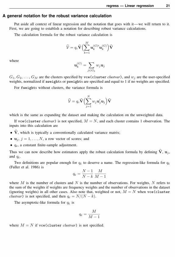
A general notation for the robust variance calculation

Put aside all context of linear regression and the notation that goes with it—we will return to it.First, we are going to establish a notation for describing robust variance calculations.

The calculation formula for the robust variance calculation is

V = qcV( M∑

k=1

u(G)′k u(G)

k

)V

whereu(G)

k =∑

j∈Gk

wjuj

G1, G2, . . . , GM are the clusters specified by vce(cluster clustvar), and wj are the user-specifiedweights, normalized if aweights or pweights are specified and equal to 1 if no weights are specified.

For fweights without clusters, the variance formula is

V = qcV( N∑

j=1

wju′juj

)V

which is the same as expanding the dataset and making the calculation on the unweighted data.

If vce(cluster clustvar) is not specified, M = N , and each cluster contains 1 observation. Theinputs into this calculation are

• V, which is typically a conventionally calculated variance matrix;

• uj , j = 1, . . . , N , a row vector of scores; and

• qc, a constant finite-sample adjustment.

Thus we can now describe how estimators apply the robust calculation formula by defining V, uj ,and qc.

Two definitions are popular enough for qc to deserve a name. The regression-like formula for qc(Fuller et al. 1986) is

qc =N − 1N − k

M

M − 1

where M is the number of clusters and N is the number of observations. For weights, N refers tothe sum of the weights if weights are frequency weights and the number of observations in the dataset(ignoring weights) in all other cases. Also note that, weighted or not, M = N when vce(clusterclustvar) is not specified, and then qc = N/(N − k).

The asymptotic-like formula for qc is

qc =M

M − 1

where M = N if vce(cluster clustvar) is not specified.


See [U] 20.20 Obtaining robust variance estimates and [P] robust for a discussion of the robustvariance estimator and a development of these formulas.

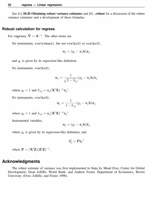
Robust calculation for regress

For regress, V = A−1. The other terms are

No instruments, vce(robust), but not vce(hc2) or vce(hc3),

uj = (yj − xjb)xj

and qc is given by its regression-like definition.

No instruments, vce(hc2),

uj =1√

1− hjj

(yj − xjb)xj

where qc = 1 and hjj = xj(X′X)−1xj′.

No instruments, vce(hc3),

uj =1

1− hjj(yj − xjb)xj

where qc = 1 and hjj = xj(X′X)−1xj′.

Instrumental variables,uj = (yj − xjb)xj

where qc is given by its regression-like definition, and

x′j = Pzj′

where P = (X′Z)(Z′Z)−1.

AcknowledgmentsThe robust estimate of variance was first implemented in Stata by Mead Over, Center for Global

Development; Dean Jolliffe, World Bank; and Andrew Foster, Department of Economics, BrownUniversity (Over, Jolliffe, and Foster 1996).

regress — Linear regression 23� �The history of regression is long and complicated: the books by Stigler (1986) and Hald (1998) aredevoted largely to the story. Legendre published first on least squares in 1805. Gauss publishedlater in 1809, but he had the idea earlier. Gauss, and especially Laplace, tied least squares to anormal errors assumption. The idea of the normal distribution can itself be traced back to DeMoivre in 1733. Laplace discussed a variety of other estimation methods and error assumptionsover his long career, while linear models long predate either innovation. Most of this work waslinked to problems in astronomy and geodesy.

A second wave of ideas started when Galton used graphical and descriptive methods on data bearingon heredity to develop what he called regression. His term reflects the common phenomenon thatcharacteristics of offspring are positively correlated with those of parents but with regression slopesuch that offspring “regress toward the mean”. Galton’s work was rather intuitive: contributionsfrom Pearson, Edgeworth, Yule, and others introduced more formal machinery, developed relatedideas on correlation, and extended application into the biological and social sciences. So mostof the elements of regression as we know it were in place by 1900.

Pierre-Simon Laplace (1749–1827) was born in Normandy and was early recognized as aremarkable mathematician. He weathered a changing political climate well enough to rise toMinister of the Interior under Napoleon in 1799 (although only for 6 weeks) and to be madea Marquis by Louis XVIII in 1817. He made many contributions to mathematics and physics,his two main interests being theoretical astronomy and probability theory (including statistics).Laplace transforms are named for him.

Adrien-Marie Legendre (1752–1833) was born in Paris (or possibly in Toulouse) and educated inmathematics and physics. He worked in number theory, geometry, differential equations, calculus,function theory, applied mathematics, and geodesy. The Legendre polynomials are named forhim. His main contribution to statistics is as one of the discoverers of least squares. He died inpoverty, having refused to bow to political pressures.

Johann Carl Friedrich Gauss (1777–1855) was born in Braunschweig (Brunswick), now inGermany. He studied there and at Gottingen. His doctoral dissertation at the University ofHelmstedt was a discussion of the fundamental theorem of algebra. He made many fundamentalcontributions to geometry, number theory, algebra, real analysis, differential equations, numericalanalysis, statistics, astronomy, optics, geodesy, mechanics, and magnetism. An outstanding genius,Gauss worked mostly in isolation in Gottingen.

Francis Galton (1822–1911) was born in Birmingham, England, into a well-to-do family withmany connections: he and Charles Darwin were first cousins. After an unsuccessful foray intomedicine, he became independently wealthy at the death of his father. Galton traveled widelyin Europe, the Middle East, and Africa, and became celebrated as an explorer and geographer.His pioneering work on weather maps helped in the identification of anticyclones, which henamed. From about 1865, most of his work was centered on quantitative problems in biology,anthropology, and psychology. In a sense, Galton (re)invented regression, and he certainly namedit. Galton also promoted the normal distribution, correlation approaches, and the use of medianand selected quantiles as descriptive statistics. He was knighted in 1909.� �

ReferencesAdkins, L. C., and R. C. Hill. 2008. Using Stata for Principles of Econometrics. 3rd ed. Hoboken, NJ: Wiley.

Alexandersson, A. 1998. gr32: Confidence ellipses. Stata Technical Bulletin 46: 10–13. Reprinted in Stata TechnicalBulletin Reprints, vol. 8, pp. 54–57. College Station, TX: Stata Press.


Angrist, J. D., and J.-S. Pischke. 2009. Mostly Harmless Econometrics: An Empiricist’s Companion. Princeton, NJ:Princeton University Press.

Cameron, A. C., and P. K. Trivedi. 2010. Microeconometrics Using Stata. Rev. ed. College Station, TX: Stata Press.

Chatterjee, S., and A. S. Hadi. 2006. Regression Analysis by Example. 4th ed. New York: Wiley.

Davidson, R., and J. G. MacKinnon. 1993. Estimation and Inference in Econometrics. New York: Oxford UniversityPress.

. 2004. Econometric Theory and Methods. New York: Oxford University Press.

Dohoo, I., W. Martin, and H. Stryhn. 2010. Veterinary Epidemiologic Research. 2nd ed. Charlottetown, Prince EdwardIsland: VER Inc.

Draper, N., and H. Smith. 1998. Applied Regression Analysis. 3rd ed. New York: Wiley.

Dunnington, G. W. 1955. Gauss: Titan of Science. New York: Hafner Publishing.

Duren, P. 2009. Changing faces: The mistaken portrait of Legendre. Notices of the American Mathematical Society56: 1440–1443.

Fuller, W. A., W. J. Kennedy, Jr., D. Schnell, G. Sullivan, and H. J. Park. 1986. PC CARP. Software package. Ames,IA: Statistical Laboratory, Iowa State University.

Gillham, N. W. 2001. A Life of Sir Francis Galton: From African Exploration to the Birth of Eugenics. New York:Oxford University Press.

Gillispie, C. C. 1997. Pierre-Simon Laplace, 1749–1827: A Life in Exact Science. Princeton: Princeton UniversityPress.

Gould, W. W. 2011. Understanding matrices intuitively, part 1. The Stata Blog: Not Elsewhere Classified.http://blog.stata.com/2011/03/03/understanding-matrices-intuitively-part-1/

Greene, W. H. 2012. Econometric Analysis. 7th ed. Upper Saddle River, NJ: Prentice Hall.

Hald, A. 1998. A History of Mathematical Statistics from 1750 to 1930. New York: Wiley.

Hamilton, L. C. 2009. Statistics with Stata (Updated for Version 10). Belmont, CA: Brooks/Cole.

Hill, R. C., W. E. Griffiths, and G. C. Lim. 2011. Principles of Econometrics. 4th ed. Hoboken, NJ: Wiley.

Kmenta, J. 1997. Elements of Econometrics. 2nd ed. Ann Arbor: University of Michigan Press.

Kohler, U., and F. Kreuter. 2009. Data Analysis Using Stata. 2nd ed. College Station, TX: Stata Press.

Long, J. S., and J. Freese. 2000. sg152: Listing and interpreting transformed coefficients from certain regressionmodels. Stata Technical Bulletin 57: 27–34. Reprinted in Stata Technical Bulletin Reprints, vol. 10, pp. 231–240.College Station, TX: Stata Press.

MacKinnon, J. G., and H. White. 1985. Some heteroskedasticity-consistent covariance matrix estimators with improvedfinite sample properties. Journal of Econometrics 29: 305–325.

Mosteller, F., and J. W. Tukey. 1977. Data Analysis and Regression: A Second Course in Statistics. Reading, MA:Addison–Wesley.

Over, M., D. Jolliffe, and A. Foster. 1996. sg46: Huber correction for two-stage least squares estimates. Stata TechnicalBulletin 29: 24–25. Reprinted in Stata Technical Bulletin Reprints, vol. 5, pp. 140–142. College Station, TX: StataPress.

Peracchi, F. 2001. Econometrics. Chichester, UK: Wiley.

Plackett, R. L. 1972. Studies in the history of probability and statistics: XXIX. The discovery of the method of leastsquares. Biometrika 59: 239–251.

Rogers, W. H. 1991. smv2: Analyzing repeated measurements—some practical alternatives. Stata Technical Bulletin4: 10–16. Reprinted in Stata Technical Bulletin Reprints, vol. 1, pp. 123–131. College Station, TX: Stata Press.

Royston, P., and G. Ambler. 1998. sg79: Generalized additive models. Stata Technical Bulletin 42: 38–43. Reprintedin Stata Technical Bulletin Reprints, vol. 7, pp. 217–224. College Station, TX: Stata Press.

Schonlau, M. 2005. Boosted regression (boosting): An introductory tutorial and a Stata plugin. Stata Journal 5:330–354.

Stigler, S. M. 1986. The History of Statistics: The Measurement of Uncertainty before 1900. Cambridge, MA: BelknapPress.


Tyler, J. H. 1997. sg73: Table making programs. Stata Technical Bulletin 40: 18–23. Reprinted in Stata TechnicalBulletin Reprints, vol. 7, pp. 186–192. College Station, TX: Stata Press.

Weesie, J. 1998. sg77: Regression analysis with multiplicative heteroscedasticity. Stata Technical Bulletin 42: 28–32.Reprinted in Stata Technical Bulletin Reprints, vol. 7, pp. 204–210. College Station, TX: Stata Press.

Weisberg, S. 2005. Applied Linear Regression. 3rd ed. New York: Wiley.

Wooldridge, J. M. 2009. Introductory Econometrics: A Modern Approach. 4th ed. Cincinnati, OH: South-Western.

. 2010. Econometric Analysis of Cross Section and Panel Data. 2nd ed. Cambridge, MA: MIT Press.

Zimmerman, F. 1998. sg93: Switching regressions. Stata Technical Bulletin 45: 30–33. Reprinted in Stata TechnicalBulletin Reprints, vol. 8, pp. 183–186. College Station, TX: Stata Press.

Also see[R] regress postestimation — Postestimation tools for regress

[R] regress postestimation time series — Postestimation tools for regress with time series

[R] anova — Analysis of variance and covariance

[R] contrast — Contrasts and linear hypothesis tests after estimation

[MI] estimation — Estimation commands for use with mi estimate

[SVY] svy estimation — Estimation commands for survey data

Stata Structural Equation Modeling Reference Manual

[U] 20 Estimation and postestimation commands

Documents

regress — Linear regression · vce(hc3) produces conﬁdence intervals that tend to be even more conservative. See Davidson and MacKinnon (1993, 554–556) and Angrist and Pischke