Embed Size (px)
Citation preview
INTERNATIONAL JOURNAL FOR NUMERICAL METHODS IN ENGINEERINGInt. J. Numer. Meth. Engng 2012; 91:269–288Published online 13 June 2012 in Wiley Online Library (wileyonlinelibrary.com). DOI: 10.1002/nme.4262
Regularized Dirac delta functions for phase field models
Hyun Geun Lee and Junseok Kim*,†
Department of Mathematics, Korea University, Seoul 136-701, Korea
SUMMARY
The phase field model is a highly successful computational technique for capturing the evolution and topo-logical change of complex interfaces. The main computational advantage of phase field models is that anexplicit tracking of the interface is unnecessary. The regularized Dirac delta function is an important ingre-dient in many interfacial problems that phase field models have been applied. The delta function can be usedto postprocess the phase field solution and represent the surface tension force. In this paper, we present andcompare various types of delta functions for phase field models. In particular, we analytically show whichtype of delta function works relatively well regardless of whether an interfacial phase transition is com-pressed or stretched. Numerical experiments are presented to show the performance of each delta function.Numerical results indicate that (1) all of the considered delta functions have good performances when thephase field is locally equilibrated; and (2) a delta function, which is the absolute value of the gradient of thephase field, is the best in most of the numerical experiments. Copyright © 2012 John Wiley & Sons, Ltd.
Received 27 November 2010; Revised 27 September 2011; Accepted 28 November 2011
KEY WORDS: regularized Dirac delta function; phase field model; Cahn–Hilliard equation; Navier–Stokesequation
1. INTRODUCTION
Multiphase fluid flows are used in a wide variety of applications such as extractors [1], polymer-dispersed liquid crystals [2], polymer blends [3], reactors [4], separators [5], sprays [6], andmicrofluidic technology [7, 8]. The fluids with changes in the interface topology are complex withdensity, diffusivity, viscosity, and surface tension. The fluids play important roles in the transi-tion process and affect both the post-transition structure of the flows and the dynamics of thetransition itself. The transition typically results from the competition between flow instabilities(e.g., due to shear or density stratification) and stabilizing influences (e.g., due to surface tensionand/or viscosity). For this reason, modeling and numerical simulation of multiphase fluid flows is agreat challenge.
In simulating multiphase fluid flows, there are two main approaches: interface tracking andinterface capturing. In interface tracking methods (front tracking [9, 10] and immersed boundary[11, 12]), Lagrangian particles are used to track the interface and are advected by the velocityfield. In interface capturing methods (volume of fluid [VOF] [11, 13, 14], level set [15–18], andphase field [19–22]), the interface is implicitly captured by a contour of a particular scalar function.Many numerical techniques, including immersed boundary [23–30], VOF [31–40], and level set[41–48], use the concept of a regularized Dirac delta function to account for interfacial effects (thisis described in more detail in Section 2), and many previous studies show that an appropriate deltafunction is required to obtain more accurate results. However, despite the large body of researchon delta functions, the performance of delta functions for phase field models has not been clearly
*Correspondence to: Junseok Kim, Department of Mathematics, Korea University, Seoul 136-701, Korea.†E-mail: [email protected]
Copyright © 2012 John Wiley & Sons, Ltd.
270 H. G. LEE AND J. KIM
addressed and compared. The purpose of this paper is to investigate the performance of regular-ized Dirac delta functions as a postprocessing of the phase field solution and a representation of thesurface tension force for phase field models in interfacial flows undergoing topological transitions.
In a phase field model, the quantity c.x, t / is defined to be the mass concentration of one of thecomponents. The Cahn–Hilliard (CH) equation was introduced to model spinodal decompositionand coarsening phenomena in binary alloys [49, 50]:
@c.x, t /
@tDM��.c.x, t //, x 2�, 0 < t 6 T , (1)
�.c.x, t //D F 0.c.x, t //� �2�c.x, t /, (2)
where � � Rd .d D 1, 2, 3/. The coefficient M represents a constant mobility. We set M � 1 forconvenience. This equation arises from the Ginzburg–Landau free energy
E.c/ WDZ�
�F.c/C
�2
2jrcj2
�dx, (3)
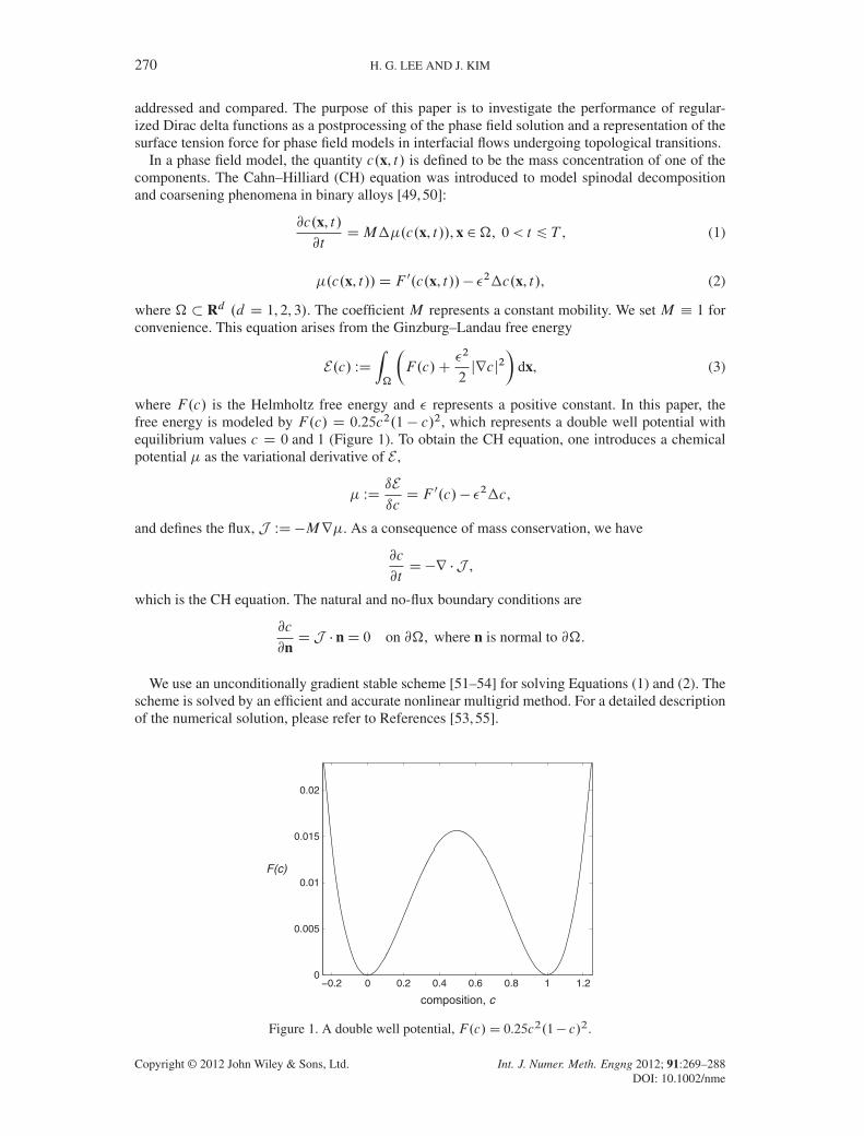
where F.c/ is the Helmholtz free energy and � represents a positive constant. In this paper, thefree energy is modeled by F.c/ D 0.25c2.1 � c/2, which represents a double well potential withequilibrium values c D 0 and 1 (Figure 1). To obtain the CH equation, one introduces a chemicalpotential � as the variational derivative of E ,
� WDıEıcD F 0.c/� �2�c,
and defines the flux, J WD �Mr�. As a consequence of mass conservation, we have
@c
@tD�r �J ,
which is the CH equation. The natural and no-flux boundary conditions are
@c
@nD J � nD 0 on @�, where n is normal to @�.
We use an unconditionally gradient stable scheme [51–54] for solving Equations (1) and (2). Thescheme is solved by an efficient and accurate nonlinear multigrid method. For a detailed descriptionof the numerical solution, please refer to References [53, 55].
−0.2 0 0.2 0.4 0.6 0.8 1 1.20
0.005
0.01
0.015
0.02
composition, c
F(c)
Figure 1. A double well potential, F.c/D 0.25c2.1� c/2.
Copyright © 2012 John Wiley & Sons, Ltd. Int. J. Numer. Meth. Engng 2012; 91:269–288DOI: 10.1002/nme
DELTA FUNCTIONS FOR PHASE FIELD MODELS 271
This paper is organized as follows. In Section 2, we review the numerical methods for regularizedDirac delta functions. We present various types of delta functions for phase field models and analyzefeature of delta functions by the interface profile in Section 3. Numerical experiments are describedin Section 4. In Section 5 conclusions are given.
2. REVIEW OF NUMERICAL METHODS FOR REGULARIZED DIRAC DELTAFUNCTIONS
We briefly review the numerical methods for regularized Dirac delta functions. Delta functions withimmersed boundary [23–30], VOF [31–40], and level set [41–48] have been intensively studied.
2.1. Immersed boundary method
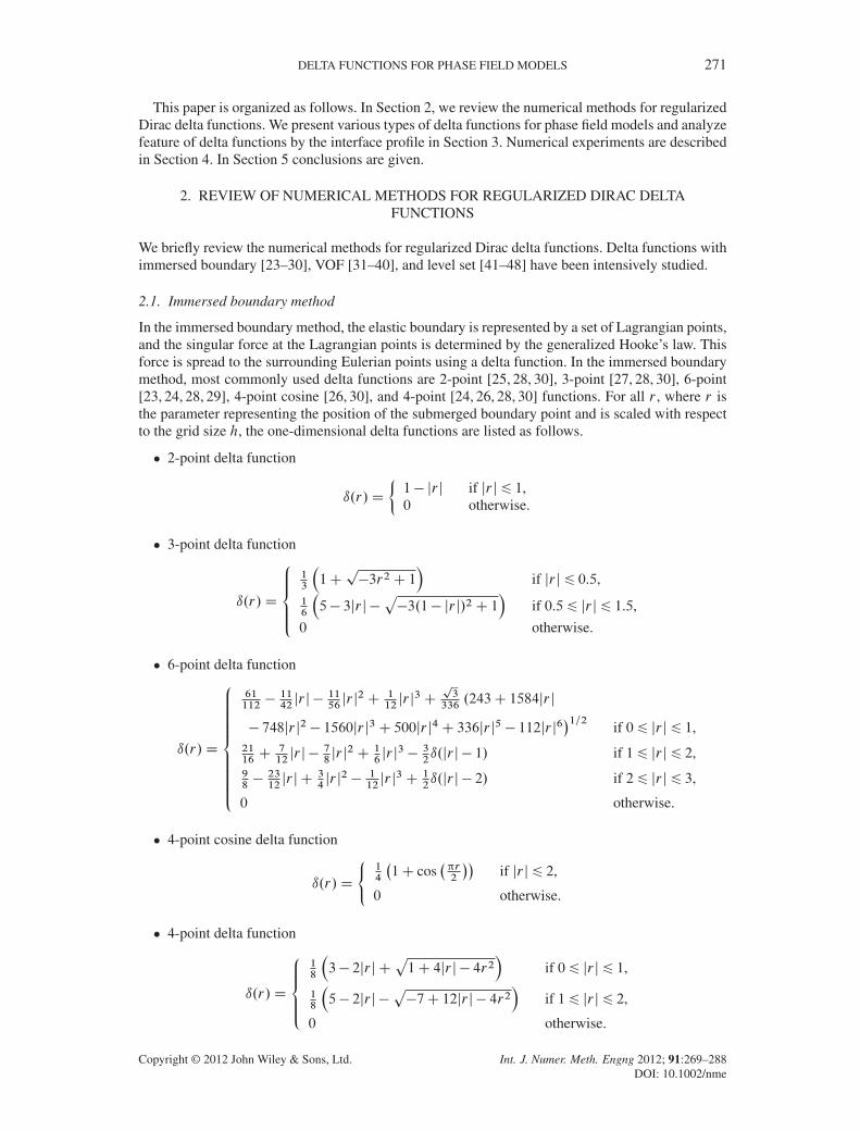
In the immersed boundary method, the elastic boundary is represented by a set of Lagrangian points,and the singular force at the Lagrangian points is determined by the generalized Hooke’s law. Thisforce is spread to the surrounding Eulerian points using a delta function. In the immersed boundarymethod, most commonly used delta functions are 2-point [25, 28, 30], 3-point [27, 28, 30], 6-point[23, 24, 28, 29], 4-point cosine [26, 30], and 4-point [24, 26, 28, 30] functions. For all r , where r isthe parameter representing the position of the submerged boundary point and is scaled with respectto the grid size h, the one-dimensional delta functions are listed as follows.
� 2-point delta function
ı.r/D
²1� jr j if jr j6 1,0 otherwise.
� 3-point delta function
ı.r/D
8̂̂<ˆ̂:
13
�1Cp�3r2C 1
�if jr j6 0.5,
16
�5� 3jr j �
p�3.1� jr j/2C 1
�if 0.56 jr j6 1.5,
0 otherwise.
� 6-point delta function
ı.r/D
8̂̂ˆ̂̂̂̂<̂ˆ̂̂̂̂ˆ̂̂:
61112� 1142jr j � 11
56jr j2C 1
12jr j3C
p3
336.243C 1584jr j
� 748jr j2 � 1560jr j3C 500jr j4C 336jr j5 � 112jr j6�1=2
if 06 jr j6 1,2116C 7
12jr j � 7
8jr j2C 1
6jr j3 � 3
2ı.jr j � 1/ if 16 jr j6 2,
98� 2312jr j C 3
4jr j2 � 1
12jr j3C 1
2ı.jr j � 2/ if 26 jr j6 3,
0 otherwise.
� 4-point cosine delta function
ı.r/D
´14
�1C cos
� r2
��if jr j6 2,
0 otherwise.
� 4-point delta function
ı.r/D
8̂̂<ˆ̂:
18
�3� 2jr j C
p1C 4jr j � 4r2
�if 06 jr j6 1,
18
�5� 2jr j �
p�7C 12jr j � 4r2
�if 16 jr j6 2,
0 otherwise.
Copyright © 2012 John Wiley & Sons, Ltd. Int. J. Numer. Meth. Engng 2012; 91:269–288DOI: 10.1002/nme
272 H. G. LEE AND J. KIM
−3 −2 −1 0 1 2 3
0
0.2
0.4
0.6
0.8
1
r
δ(r)
2−point3−point6−point4−point cosine4−point
Figure 2. Five types of delta functions used in the immersed boundary method.
The aforementioned five types of delta functions are shown in Figure 2. Shin et al. [28] analyzedthe stability regimes of the feedback forcing gains in the feedback forcing method for several typesof delta functions and showed that non-growing oscillations became smaller for the delta functionsupported by more points. Yang et al. [30] found that the nonphysical oscillations are mainly becausethe derivatives of the regular discrete delta functions do not satisfy certain moment conditions anddemonstrated that the smoothed discrete delta functions can effectively suppress the nonphysicaloscillations in the volume forces and improve the accuracy of the immersed boundary method withdirect forcing in moving boundary simulations.
2.2. Volume of fluid method
The VOF method was proposed by Hirt and Nichols [56]. In VOF method, the interface is recon-structed from the values of a color function that represents the volume fraction of one of the fluids ineach cell. The continuum surface force (CSF) of Brackbill et al. [57] has been widely used to modelsurface tension in multiphase fluid flows in VOF method. In the CSF model [33, 34, 40, 58–61], thesurface tension force is converted into a volume force via a delta function, fD ��nı, where � is thesurface tension coefficient, � is the curvature, n is the normal to the surface, and ı is a delta function.In VOF method, the most commonly used delta function is ı. Qc/D jr Qcj, where Qc is a smoothed ver-sion of the volume fraction. The CSF model is simple and robust, and it involves only the solving ofa field equation for a smoothed phase field Qc. However, the method is known to produce strong andspurious currents near the interface. For this reason, many researchers have developed new methodsto reduce spurious currents [37, 40, 62–64]. Meier et al. [37] reduced spurious currents using thepiecewise-linear interface construction VOF method. In Reference [64], a parabolic reconstructionof surface tension algorithm is used to gain higher-order accuracy for the surface tension force.
2.3. Level set method
In the level set method, first devised and introduced by Osher and Sethian [65], delta functions areoften used to distribute a singular force or to compute a surface area [46, 66–68]. Most commonlyused delta functions are listed as follows. Here, � is proportional to the grid size, that is, � Dmh fora positive number m.
� Delta function in References [41, 43, 45, 47, 48]
ı�.x/D
´1�
�1�
ˇ̌x�
ˇ̌�if jxj6 �,
0 otherwise.
Copyright © 2012 John Wiley & Sons, Ltd. Int. J. Numer. Meth. Engng 2012; 91:269–288DOI: 10.1002/nme
DELTA FUNCTIONS FOR PHASE FIELD MODELS 273
� Delta function in References [41–44, 46–48]
ı�.x/D
´12�
�1C cos
� x�
��if jxj6 �,
0 otherwise.
Tornberg and Engquist [69] pointed out that the most common technique for regularization ofdelta functions in level set simulations is not consistent and analyzed the accuracy of regularizationof delta functions. Smereka [45] presented methods for constructing consistent approximations toDirac delta measures concentrated on piecewise smooth curves or surfaces. Towers [70] proposedsecond-order finite difference methods for approximating Heaviside functions and showed that themethods are more accurate than a commonly used approximate Heaviside function.
3. REGULARIZED DIRAC DELTA FUNCTIONS FOR PHASE FIELD MODELS
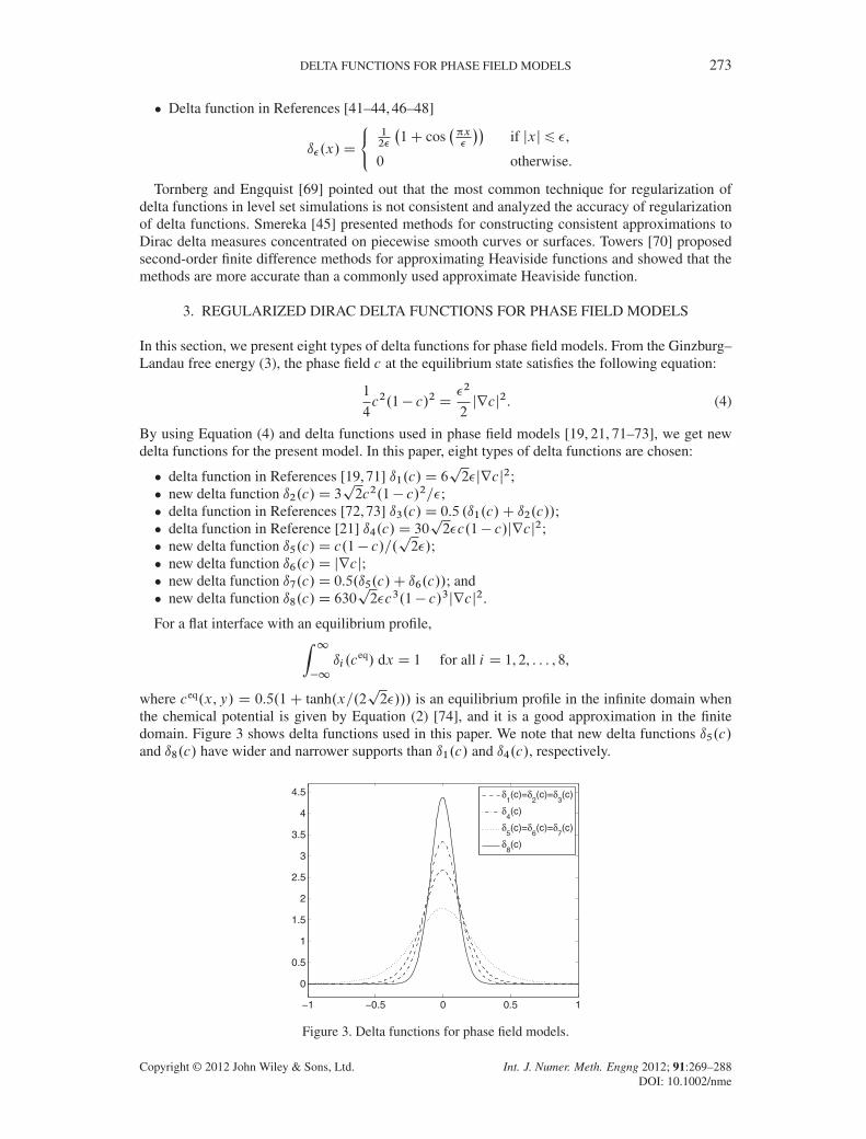
In this section, we present eight types of delta functions for phase field models. From the Ginzburg–Landau free energy (3), the phase field c at the equilibrium state satisfies the following equation:
1
4c2.1� c/2 D
�2
2jrcj2. (4)
By using Equation (4) and delta functions used in phase field models [19, 21, 71–73], we get newdelta functions for the present model. In this paper, eight types of delta functions are chosen:
� delta function in References [19, 71] ı1.c/D 6p2�jrcj2;
� new delta function ı2.c/D 3p2c2.1� c/2=�;
� delta function in References [72, 73] ı3.c/D 0.5 .ı1.c/C ı2.c//;� delta function in Reference [21] ı4.c/D 30
p2�c.1� c/jrcj2;
� new delta function ı5.c/D c.1� c/=.p2�/;
� new delta function ı6.c/D jrcj;� new delta function ı7.c/D 0.5.ı5.c/C ı6.c//; and� new delta function ı8.c/D 630
p2�c3.1� c/3jrcj2.
For a flat interface with an equilibrium profile,Z 1�1
ıi .ceq/ dx D 1 for all i D 1, 2, : : : , 8,
where ceq.x,y/ D 0.5.1C tanh.x=.2p2�/// is an equilibrium profile in the infinite domain when
the chemical potential is given by Equation (2) [74], and it is a good approximation in the finitedomain. Figure 3 shows delta functions used in this paper. We note that new delta functions ı5.c/and ı8.c/ have wider and narrower supports than ı1.c/ and ı4.c/, respectively.
−1 −0.5 0 0.5 1
0
0.5
1
1.5
2
2.5
3
3.5
4
4.5 δ1(c)=δ
2(c)=δ
3(c)
δ4(c)
δ5(c)=δ
6(c)=δ
7(c)
δ8(c)
Figure 3. Delta functions for phase field models.
Copyright © 2012 John Wiley & Sons, Ltd. Int. J. Numer. Meth. Engng 2012; 91:269–288DOI: 10.1002/nme
274 H. G. LEE AND J. KIM
We now consider a line of unit length on a unit domain �D .0, 1/� .0, 1/:
c.x,y/D1
2
�1C tanh
�0.5� x
2p2a
��(5)
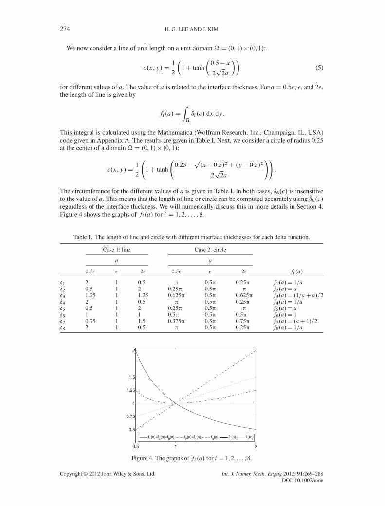
for different values of a. The value of a is related to the interface thickness. For aD 0.5�, �, and 2�,the length of line is given by
fi .a/D
Z�
ıi .c/ dx dy.
This integral is calculated using the Mathematica (Wolfram Research, Inc., Champaign, IL, USA)code given in Appendix A. The results are given in Table I. Next, we consider a circle of radius 0.25at the center of a domain �D .0, 1/� .0, 1/:
c.x, y/D1
2
1C tanh
0.25�
p.x � 0.5/2C .y � 0.5/2
2p2a
!!.
The circumference for the different values of a is given in Table I. In both cases, ı6.c/ is insensitiveto the value of a. This means that the length of line or circle can be computed accurately using ı6.c/regardless of the interface thickness. We will numerically discuss this in more details in Section 4.Figure 4 shows the graphs of fi .a/ for i D 1, 2, : : : , 8.
Table I. The length of line and circle with different interface thicknesses for each delta function.
Case 1: line Case 2: circle
a a
0.5� � 2� 0.5� � 2� fi .a/
ı1 2 1 0.5 0.5 0.25 f1.a/D 1=aı2 0.5 1 2 0.25 0.5 f2.a/D aı3 1.25 1 1.25 0.625 0.5 0.625 f3.a/D .1=aC a/=2ı4 2 1 0.5 0.5 0.25 f4.a/D 1=aı5 0.5 1 2 0.25 0.5 f5.a/D aı6 1 1 1 0.5 0.5 0.5 f6.a/D 1ı7 0.75 1 1.5 0.375 0.5 0.75 f7.a/D .aC 1/=2ı8 2 1 0.5 0.5 0.25 f8.a/D 1=a
0.5 1 2
0.5
0.75
1
1.25
1.5
2
f1(a)=f
4(a)=f
8(a) f
2(a)=f
5(a) f
3(a) f
6(a) f
7(a)
Figure 4. The graphs of fi .a/ for i D 1, 2, : : : , 8.
Copyright © 2012 John Wiley & Sons, Ltd. Int. J. Numer. Meth. Engng 2012; 91:269–288DOI: 10.1002/nme
DELTA FUNCTIONS FOR PHASE FIELD MODELS 275
4. NUMERICAL EXPERIMENTS
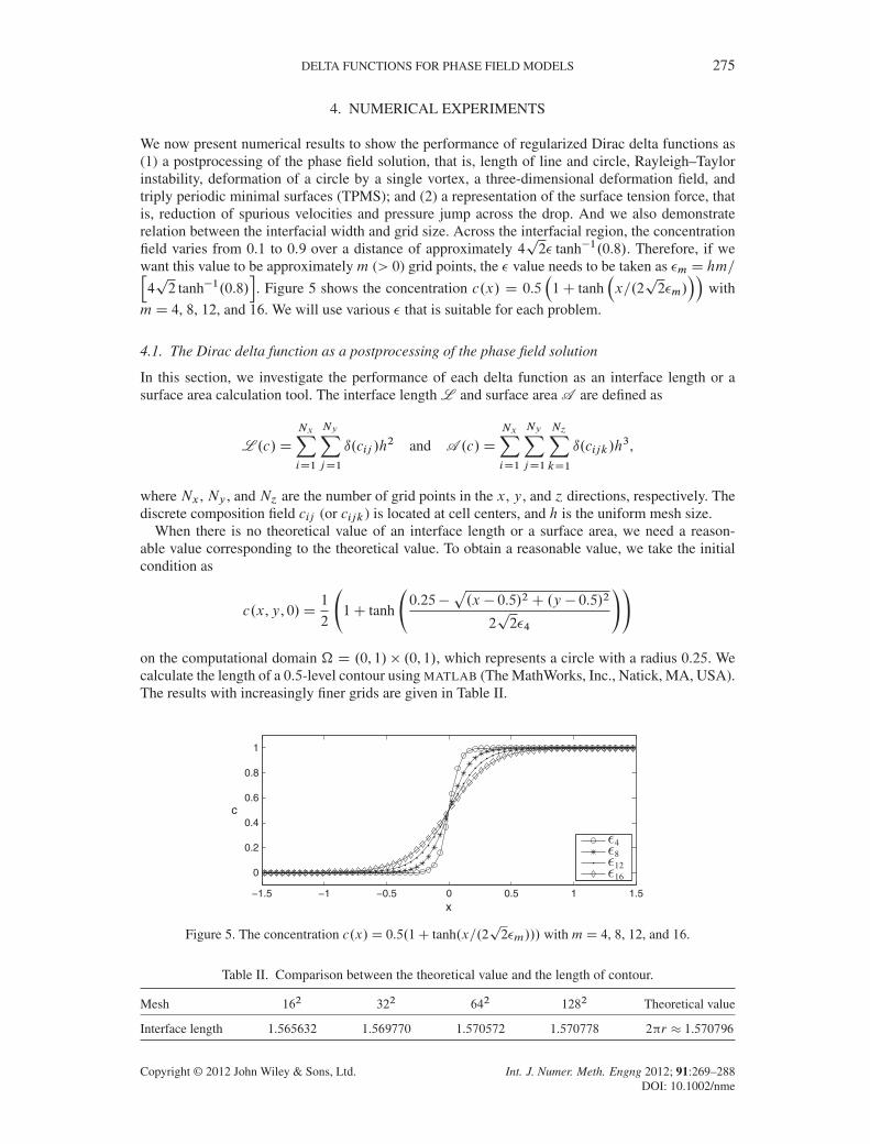
We now present numerical results to show the performance of regularized Dirac delta functions as(1) a postprocessing of the phase field solution, that is, length of line and circle, Rayleigh–Taylorinstability, deformation of a circle by a single vortex, a three-dimensional deformation field, andtriply periodic minimal surfaces (TPMS); and (2) a representation of the surface tension force, thatis, reduction of spurious velocities and pressure jump across the drop. And we also demonstraterelation between the interfacial width and grid size. Across the interfacial region, the concentrationfield varies from 0.1 to 0.9 over a distance of approximately 4
p2� tanh�1.0.8/. Therefore, if we
want this value to be approximatelym (> 0) grid points, the � value needs to be taken as �m D hm=h4p2 tanh�1.0.8/
i. Figure 5 shows the concentration c.x/ D 0.5
�1C tanh
�x=.2p2�m/
��with
mD 4, 8, 12, and 16. We will use various � that is suitable for each problem.
4.1. The Dirac delta function as a postprocessing of the phase field solution
In this section, we investigate the performance of each delta function as an interface length or asurface area calculation tool. The interface length L and surface area A are defined as
L .c/D
NxXiD1
NyXjD1
ı.cij /h2 and A .c/D
NxXiD1
NyXjD1
N´XkD1
ı.cijk/h3,
where Nx , Ny , and N´ are the number of grid points in the x, y, and ´ directions, respectively. Thediscrete composition field cij (or cijk) is located at cell centers, and h is the uniform mesh size.
When there is no theoretical value of an interface length or a surface area, we need a reason-able value corresponding to the theoretical value. To obtain a reasonable value, we take the initialcondition as
c.x,y, 0/D1
2
1C tanh
0.25�
p.x � 0.5/2C .y � 0.5/2
2p2�4
!!
on the computational domain � D .0, 1/ � .0, 1/, which represents a circle with a radius 0.25. Wecalculate the length of a 0.5-level contour using MATLAB (The MathWorks, Inc., Natick, MA, USA).The results with increasingly finer grids are given in Table II.
−1.5 −1 −0.5 0 0.5 1 1.5
0
0.2
0.4
0.6
0.8
1
x
c
481216
Figure 5. The concentration c.x/D 0.5.1C tanh.x=.2p2�m/// with mD 4, 8, 12, and 16.
Table II. Comparison between the theoretical value and the length of contour.
Mesh 162 322 642 1282 Theoretical value
Interface length 1.565632 1.569770 1.570572 1.570778 2 r � 1.570796
Copyright © 2012 John Wiley & Sons, Ltd. Int. J. Numer. Meth. Engng 2012; 91:269–288DOI: 10.1002/nme
276 H. G. LEE AND J. KIM
Table III. Comparison between the theoretical value and the area of isosurface.
Mesh 323 643 1283 2563 Theoretical value
Surface area 0.781695 0.784493 0.785185 0.785364 4 r2 � 0.785398
Next, the initial condition is
c.x,y, ´, 0/D1
2
1C tanh
0.25�
p.x � 0.5/2C .y � 0.5/2C .´� 0.5/2
2p2�4
!!
on � D .0, 1/ � .0, 1/ � .0, 1/, which represents a sphere with a radius 0.25. We compute the areaof an isosurface by summation of the areas of all triangle tiles in the isosurface using MATLAB. Theresults with increasingly finer grids are given in Table III. The results in Tables II and III suggestthat the length of contour and the area of isosurface agree well with the theoretical value.
4.1.1. Test 1: length of line and circle. In Section 3, we explored the performance of delta functionsby the interface profile using Mathematica. To numerically explore the performance, we considertwo initial conditions on �D .0, 1/� .0, 1/:
c.x, y, 0/D1
2
�1C tanh
�0.5� x
2p2a
��and
c.x, y, 0/D1
2
1C tanh
0.25�
p.x � 0.5/2C .y � 0.5/2
2p2a
!!
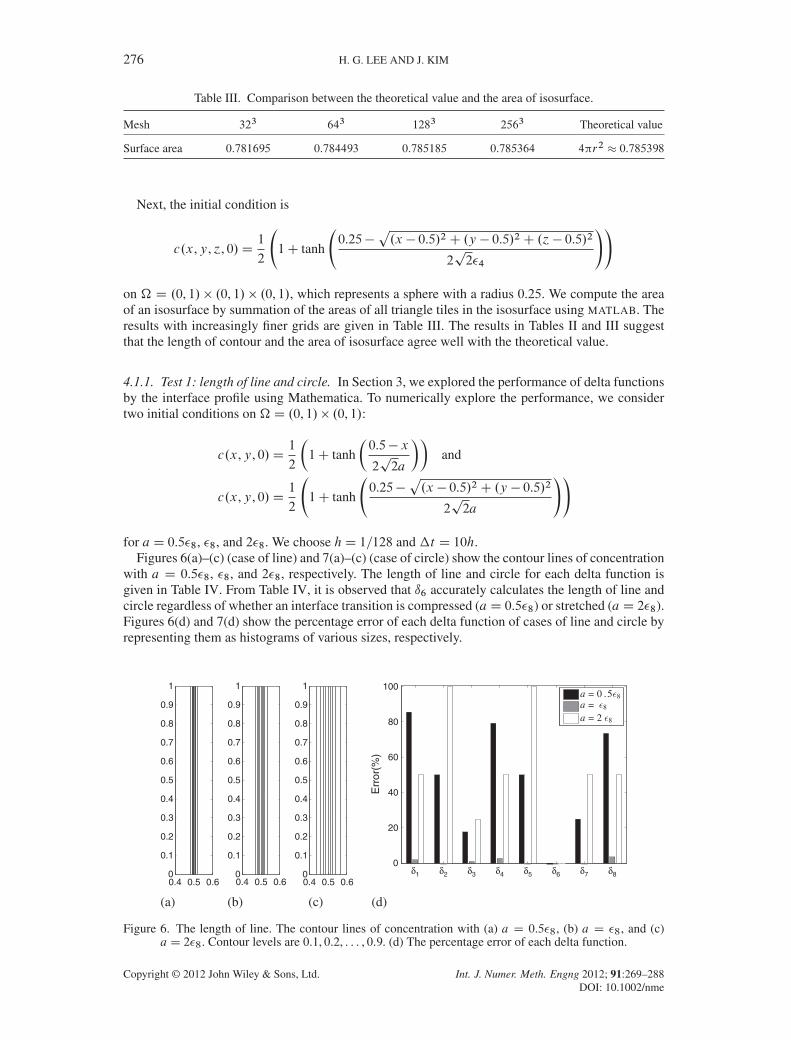
for aD 0.5�8, �8, and 2�8. We choose hD 1=128 and �t D 10h.Figures 6(a)–(c) (case of line) and 7(a)–(c) (case of circle) show the contour lines of concentration
with a D 0.5�8, �8, and 2�8, respectively. The length of line and circle for each delta function isgiven in Table IV. From Table IV, it is observed that ı6 accurately calculates the length of line andcircle regardless of whether an interface transition is compressed (aD 0.5�8) or stretched (aD 2�8).Figures 6(d) and 7(d) show the percentage error of each delta function of cases of line and circle byrepresenting them as histograms of various sizes, respectively.
0.4 0.5 0.60
0.1
0.2
0.3
0.4
0.5
0.6
0.7
0.8
0.9
1
(a)
0.4 0.5 0.60
0.1
0.2
0.3
0.4
0.5
0.6
0.7
0.8
0.9
1
(b)
0.4 0.5 0.60
0.1
0.2
0.3
0.4
0.5
0.6
0.7
0.8
0.9
1
(c)
0
20
40
60
80
100
Err
or(%
)
δ1 δ2 δ3 δ4 δ5 δ6 δ7 δ8
a = 0 .5 8a = 8
a = 2 8
(d)
Figure 6. The length of line. The contour lines of concentration with (a) a D 0.5�8, (b) a D �8, and (c)aD 2�8. Contour levels are 0.1, 0.2, : : : , 0.9. (d) The percentage error of each delta function.
Copyright © 2012 John Wiley & Sons, Ltd. Int. J. Numer. Meth. Engng 2012; 91:269–288DOI: 10.1002/nme
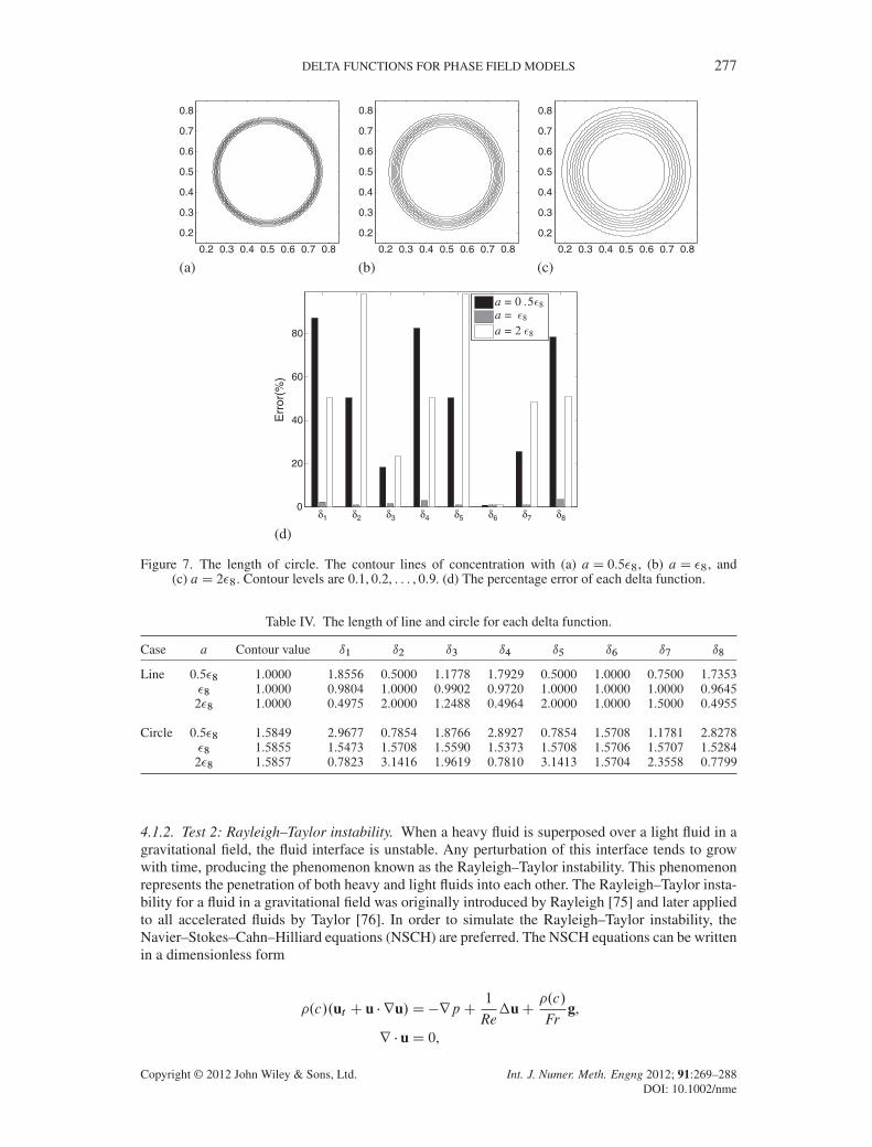
DELTA FUNCTIONS FOR PHASE FIELD MODELS 277
0.2 0.3 0.4 0.5 0.6 0.7 0.8
0.2
0.3
0.4
0.5
0.6
0.7
0.8
(a)0.2 0.3 0.4 0.5 0.6 0.7 0.8
0.2
0.3
0.4
0.5
0.6
0.7
0.8
(b)0.2 0.3 0.4 0.5 0.6 0.7 0.8
0.2
0.3
0.4
0.5
0.6
0.7
0.8
(c)
0
20
40
60
80
Err
or(%
)
δ1 δ2 δ3 δ4 δ5 δ6 δ7 δ8
a = 0 .5 8a = 8
a = 2 8
(d)
Figure 7. The length of circle. The contour lines of concentration with (a) aD 0.5�8, (b) aD �8, and(c) aD 2�8. Contour levels are 0.1, 0.2, : : : , 0.9. (d) The percentage error of each delta function.
Table IV. The length of line and circle for each delta function.
Case a Contour value ı1 ı2 ı3 ı4 ı5 ı6 ı7 ı8
Line 0.5�8 1.0000 1.8556 0.5000 1.1778 1.7929 0.5000 1.0000 0.7500 1.7353�8 1.0000 0.9804 1.0000 0.9902 0.9720 1.0000 1.0000 1.0000 0.96452�8 1.0000 0.4975 2.0000 1.2488 0.4964 2.0000 1.0000 1.5000 0.4955
Circle 0.5�8 1.5849 2.9677 0.7854 1.8766 2.8927 0.7854 1.5708 1.1781 2.8278�8 1.5855 1.5473 1.5708 1.5590 1.5373 1.5708 1.5706 1.5707 1.52842�8 1.5857 0.7823 3.1416 1.9619 0.7810 3.1413 1.5704 2.3558 0.7799
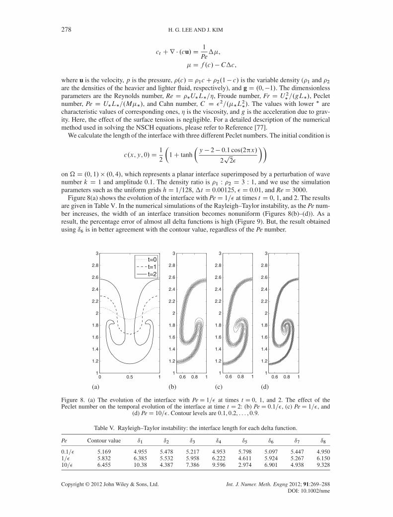
4.1.2. Test 2: Rayleigh–Taylor instability. When a heavy fluid is superposed over a light fluid in agravitational field, the fluid interface is unstable. Any perturbation of this interface tends to growwith time, producing the phenomenon known as the Rayleigh–Taylor instability. This phenomenonrepresents the penetration of both heavy and light fluids into each other. The Rayleigh–Taylor insta-bility for a fluid in a gravitational field was originally introduced by Rayleigh [75] and later appliedto all accelerated fluids by Taylor [76]. In order to simulate the Rayleigh–Taylor instability, theNavier–Stokes–Cahn–Hilliard equations (NSCH) are preferred. The NSCH equations can be writtenin a dimensionless form
.c/.ut C u � ru/D�rpC1
Re�uC
.c/
Frg,
r � uD 0,
Copyright © 2012 John Wiley & Sons, Ltd. Int. J. Numer. Meth. Engng 2012; 91:269–288DOI: 10.1002/nme
278 H. G. LEE AND J. KIM
ct Cr � .cu/D1
Pe��,
�D f .c/�C�c,
where u is the velocity, p is the pressure, .c/D 1cC 2.1� c/ is the variable density (1 and 2are the densities of the heavier and lighter fluid, respectively), and g D .0,�1/. The dimensionlessparameters are the Reynolds number, Re D �U�L�=, Froude number, Fr D U 2� =.gL�/, Pecletnumber, Pe D U�L�=.M��/, and Cahn number, C D �2=.��L
2�/. The values with lower � are
characteristic values of corresponding ones, is the viscosity, and g is the acceleration due to grav-ity. Here, the effect of the surface tension is negligible. For a detailed description of the numericalmethod used in solving the NSCH equations, please refer to Reference [77].
We calculate the length of the interface with three different Peclet numbers. The initial condition is
c.x,y, 0/D1
2
�1C tanh
�y � 2� 0.1 cos.2 x/
2p2�
��
on �D .0, 1/� .0, 4/, which represents a planar interface superimposed by a perturbation of wavenumber k D 1 and amplitude 0.1. The density ratio is 1 W 2 D 3 W 1, and we use the simulationparameters such as the uniform grids hD 1=128, �t D 0.00125, � D 0.01, and ReD 3000.
Figure 8(a) shows the evolution of the interface with PeD 1=� at times t D 0, 1, and 2. The resultsare given in Table V. In the numerical simulations of the Rayleigh–Taylor instability, as the Pe num-ber increases, the width of an interface transition becomes nonuniform (Figures 8(b)–(d)). As aresult, the percentage error of almost all delta functions is high (Figure 9). But, the result obtainedusing ı6 is in better agreement with the contour value, regardless of the Pe number.
0 0.5 11
1.2
1.4
1.6
1.8
2
2.2
2.4
2.6
2.8
3t=0t=1t=2
(a)
0.6 0.8 11
1.2
1.4
1.6
1.8
2
2.2
2.4
2.6
2.8
3
(b)
0.6 0.8 11
1.2
1.4
1.6
1.8
2
2.2
2.4
2.6
2.8
3
(c)
0.6 0.8 11
1.2
1.4
1.6
1.8
2
2.2
2.4
2.6
2.8
3
(d)
Figure 8. (a) The evolution of the interface with PeD 1=� at times t D 0, 1, and 2. The effect of thePeclet number on the temporal evolution of the interface at time t D 2: (b) PeD 0.1=�, (c) PeD 1=�, and
(d) PeD 10=�. Contour levels are 0.1, 0.2, : : : , 0.9.
Table V. Rayleigh–Taylor instability: the interface length for each delta function.
Pe Contour value ı1 ı2 ı3 ı4 ı5 ı6 ı7 ı8
0.1=� 5.169 4.955 5.478 5.217 4.953 5.798 5.097 5.447 4.9501=� 5.832 6.385 5.532 5.958 6.222 4.611 5.924 5.267 6.15010=� 6.455 10.38 4.387 7.386 9.596 2.974 6.901 4.938 9.328
Copyright © 2012 John Wiley & Sons, Ltd. Int. J. Numer. Meth. Engng 2012; 91:269–288DOI: 10.1002/nme
DELTA FUNCTIONS FOR PHASE FIELD MODELS 279
0
10
20
30
40
50
60
Err
or(%
)
δ1 δ2 δ3 δ4 δ5 δ6 δ7 δ8
Pe = 10Pe = 1Pe = 0 .1
Figure 9. Rayleigh–Taylor instability: the percentage error of each delta function.
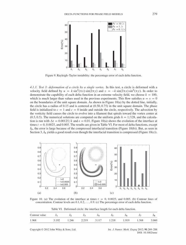
4.1.3. Test 3: deformation of a circle by a single vortex. In this test, a circle is deformed with avelocity field defined by u D k sin2. x/ sin.2 y/ and v D �k sin.2 x/ sin2. y/. In order todemonstrate the capability of each delta function in an extreme velocity field, we choose k D 100,which is much larger than values used in the previous experiments. This flow satisfies u D v D 0
on the boundaries of the unit square domain. As shown in Figure 10(a) by the dotted line, initially,the circle has a radius of 0.15 and is centered at .0.50, 0.75/ in the unit square domain. The phasefield is initialized to c D 1 and c D 0 inside and outside the circle, respectively. The advection bythe vorticity field causes the circle to evolve into a filament that spirals toward the vortex center at.0.5, 0.5/. The numerical solutions are computed on the uniform grids h D 1=128, and the calcula-tion is run with �t D 0.00125=k and � D 0.01. Figure 10(a) shows the evolution of the interface attimes t D 0, 0.0025, and 0.005. The results are given in Table VI. For most of delta functions, exceptı6, the error is large because of the compressed interfacial transition (Figure 10(b)). But, as seen inSection 3, ı6 yields a good result even though the interfacial transition is compressed (Figure 10(c)).
0.2 0.4 0.60
0.1
0.2
0.3
0.4
0.5
0.6
0.7
0.8
0.9
1
+
t=0t=0.0025t=0.005
(a)
+
0.2 0.4 0.60
0.1
0.2
0.3
0.4
0.5
0.6
0.7
0.8
0.9
1
t=0t=0.005
(b)
0
10
20
30
40
50
60
Err
or(%
)
δ1 δ2 δ3 δ4 δ5 δ6 δ7 δ8
(c)
Figure 10. (a) The evolution of the interface at times t D 0, 0.0025, and 0.005. (b) Contour lines ofconcentration. Contour levels are 0.1, 0.2, : : : , 0.9. (c) The percentage error of each delta function.
Table VI. Deformed circle: the interface length for each delta function.
Contour value ı1 ı2 ı3 ı4 ı5 ı6 ı7 ı8
1.968 3.192 1.246 2.219 3.117 1.218 1.919 1.568 3.060
Copyright © 2012 John Wiley & Sons, Ltd. Int. J. Numer. Meth. Engng 2012; 91:269–288DOI: 10.1002/nme
280 H. G. LEE AND J. KIM
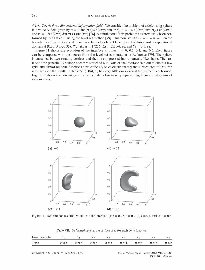
4.1.4. Test 4: three-dimensional deformation field. We consider the problem of a deforming spherein a velocity field given by uD 2 sin2. x/ sin.2 y/ sin.2 ´/, v D � sin.2 x/ sin2. y/ sin.2 ´/,and w D� sin.2 x/ sin.2 y/ sin2. ´/ [78]. A simulation of this problem has previously been per-formed by Enright et al. using the level set method [79]. This flow satisfies u D v D w D 0 on theboundaries of the unit cube domain. A sphere of radius 0.15 is placed within a unit computationaldomain at .0.35, 0.35, 0.35/. We take hD 1=256, �t D 2.5e-4, �3, and PeD 0.1=�3.
Figure 11 shows the evolution of the interface at times t D 0, 0.2, 0.4, and 0.6. Each figurecan be compared with the figures from the level set computation in Reference [79]. The sphereis entrained by two rotating vortices and then is compressed into a pancake-like shape. The sur-face of the pancake-like shape becomes stretched out. Parts of the interface thin out to about a fewgrid, and almost all delta functions have difficulty to calculate exactly the surface area of this thininterface (see the results in Table VII). But, ı6 has very little error even if the surface is deformed.Figure 12 shows the percentage error of each delta function by representing them as histograms ofvarious sizes.
(a) t = 0 (b) t = 0.2
(c) t = 0.4 (d) t = 0.6
Figure 11. Deformation test: the evolution of the interface. (a) t D 0, (b) t D 0.2, (c) t D 0.4, and (d) t D 0.6.
Table VII. Deformed sphere: the surface area for each delta function.
Isosurface value ı1 ı2 ı3 ı4 ı5 ı6 ı7 ı8
0.586 0.565 0.567 0.566 0.545 0.634 0.596 0.615 0.528
Copyright © 2012 John Wiley & Sons, Ltd. Int. J. Numer. Meth. Engng 2012; 91:269–288DOI: 10.1002/nme
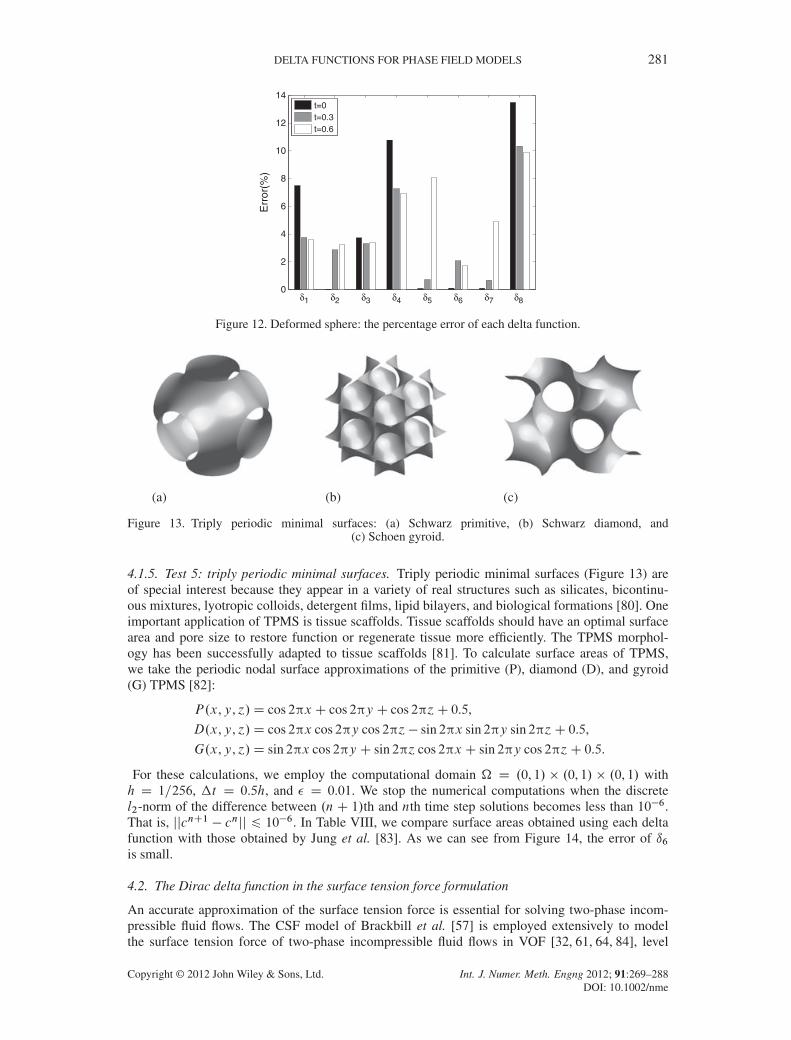
DELTA FUNCTIONS FOR PHASE FIELD MODELS 281
0
2
4
6
8
10
12
14
Err
or(%
)
δ1 δ2 δ3 δ4 δ5 δ6 δ7 δ8
t=0t=0.3t=0.6
Figure 12. Deformed sphere: the percentage error of each delta function.
(a) (b) (c)
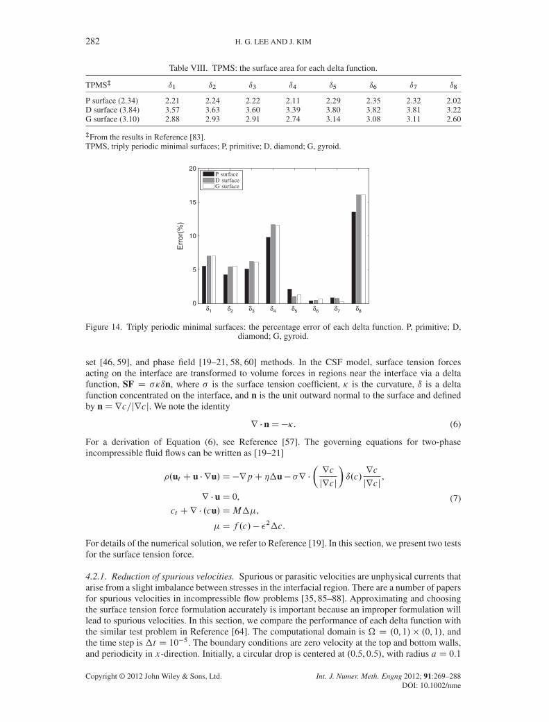
Figure 13. Triply periodic minimal surfaces: (a) Schwarz primitive, (b) Schwarz diamond, and(c) Schoen gyroid.
4.1.5. Test 5: triply periodic minimal surfaces. Triply periodic minimal surfaces (Figure 13) areof special interest because they appear in a variety of real structures such as silicates, bicontinu-ous mixtures, lyotropic colloids, detergent films, lipid bilayers, and biological formations [80]. Oneimportant application of TPMS is tissue scaffolds. Tissue scaffolds should have an optimal surfacearea and pore size to restore function or regenerate tissue more efficiently. The TPMS morphol-ogy has been successfully adapted to tissue scaffolds [81]. To calculate surface areas of TPMS,we take the periodic nodal surface approximations of the primitive (P), diamond (D), and gyroid(G) TPMS [82]:
P.x,y, ´/D cos 2 xC cos 2 y C cos 2 ´C 0.5,
D.x,y, ´/D cos 2 x cos 2 y cos 2 ´� sin 2 x sin 2 y sin 2 ´C 0.5,
G.x,y, ´/D sin 2 x cos 2 y C sin 2 ´ cos 2 xC sin 2 y cos 2 ´C 0.5.
For these calculations, we employ the computational domain � D .0, 1/ � .0, 1/ � .0, 1/ withh D 1=256, �t D 0.5h, and � D 0.01. We stop the numerical computations when the discretel2-norm of the difference between .nC 1/th and nth time step solutions becomes less than 10�6.That is, jjcnC1 � cnjj 6 10�6. In Table VIII, we compare surface areas obtained using each deltafunction with those obtained by Jung et al. [83]. As we can see from Figure 14, the error of ı6is small.
4.2. The Dirac delta function in the surface tension force formulation
An accurate approximation of the surface tension force is essential for solving two-phase incom-pressible fluid flows. The CSF model of Brackbill et al. [57] is employed extensively to modelthe surface tension force of two-phase incompressible fluid flows in VOF [32, 61, 64, 84], level
Copyright © 2012 John Wiley & Sons, Ltd. Int. J. Numer. Meth. Engng 2012; 91:269–288DOI: 10.1002/nme
282 H. G. LEE AND J. KIM
Table VIII. TPMS: the surface area for each delta function.
TPMS� ı1 ı2 ı3 ı4 ı5 ı6 ı7 ı8
P surface (2.34) 2.21 2.24 2.22 2.11 2.29 2.35 2.32 2.02D surface (3.84) 3.57 3.63 3.60 3.39 3.80 3.82 3.81 3.22G surface (3.10) 2.88 2.93 2.91 2.74 3.14 3.08 3.11 2.60
�From the results in Reference [83].TPMS, triply periodic minimal surfaces; P, primitive; D, diamond; G, gyroid.
0
5
10
15
20
Err
or(%
)
δ1 δ2 δ3 δ4 δ5 δ6 δ7 δ8
P surfaceD surfaceG surface
Figure 14. Triply periodic minimal surfaces: the percentage error of each delta function. P, primitive; D,diamond; G, gyroid.
set [46, 59], and phase field [19–21, 58, 60] methods. In the CSF model, surface tension forcesacting on the interface are transformed to volume forces in regions near the interface via a deltafunction, SF D ��ın, where � is the surface tension coefficient, � is the curvature, ı is a deltafunction concentrated on the interface, and n is the unit outward normal to the surface and definedby nDrc=jrcj. We note the identity
r � nD��. (6)
For a derivation of Equation (6), see Reference [57]. The governing equations for two-phaseincompressible fluid flows can be written as [19–21]
.ut C u � ru/D�rpC �u� �r ��rc
jrcj
�ı.c/
rc
jrcj,
r � uD 0,
ct Cr � .cu/DM��,
�D f .c/� �2�c.
(7)
For details of the numerical solution, we refer to Reference [19]. In this section, we present two testsfor the surface tension force.
4.2.1. Reduction of spurious velocities. Spurious or parasitic velocities are unphysical currents thatarise from a slight imbalance between stresses in the interfacial region. There are a number of papersfor spurious velocities in incompressible flow problems [35, 85–88]. Approximating and choosingthe surface tension force formulation accurately is important because an improper formulation willlead to spurious velocities. In this section, we compare the performance of each delta function withthe similar test problem in Reference [64]. The computational domain is � D .0, 1/ � .0, 1/, andthe time step is �t D 10�5. The boundary conditions are zero velocity at the top and bottom walls,and periodicity in x-direction. Initially, a circular drop is centered at .0.5, 0.5/, with radius a D 0.1
Copyright © 2012 John Wiley & Sons, Ltd. Int. J. Numer. Meth. Engng 2012; 91:269–288DOI: 10.1002/nme
DELTA FUNCTIONS FOR PHASE FIELD MODELS 283
and surface tension coefficient � D 0.357. Both fluids have equal density, 4, and viscosity, 1. Theinitial velocity field is zero. The exact solution is zero velocity for all time. In dimensionless terms,the relevant parameter is the Ohnesorge number OhD =
p�a 2.6463.
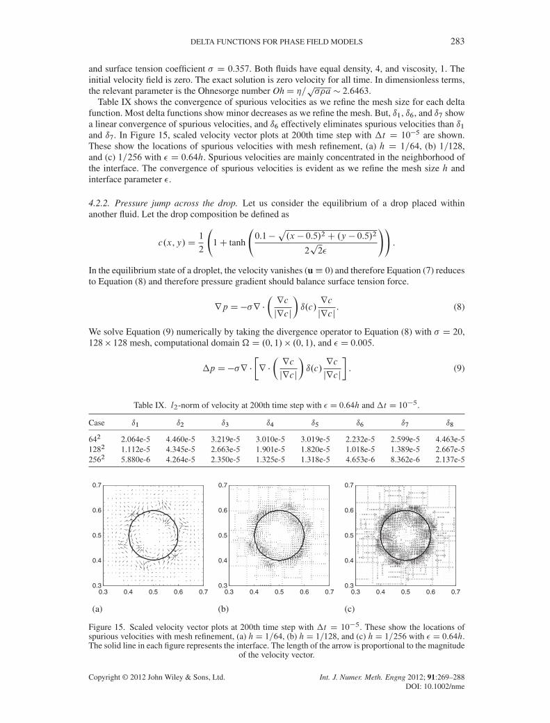
Table IX shows the convergence of spurious velocities as we refine the mesh size for each deltafunction. Most delta functions show minor decreases as we refine the mesh. But, ı1, ı6, and ı7 showa linear convergence of spurious velocities, and ı6 effectively eliminates spurious velocities than ı1and ı7. In Figure 15, scaled velocity vector plots at 200th time step with �t D 10�5 are shown.These show the locations of spurious velocities with mesh refinement, (a) h D 1=64, (b) 1=128,and (c) 1=256 with � D 0.64h. Spurious velocities are mainly concentrated in the neighborhood ofthe interface. The convergence of spurious velocities is evident as we refine the mesh size h andinterface parameter �.
4.2.2. Pressure jump across the drop. Let us consider the equilibrium of a drop placed withinanother fluid. Let the drop composition be defined as
c.x,y/D1
2
1C tanh
0.1�
p.x � 0.5/2C .y � 0.5/2
2p2�
!!.
In the equilibrium state of a droplet, the velocity vanishes (u� 0) and therefore Equation (7) reducesto Equation (8) and therefore pressure gradient should balance surface tension force.
rp D��r �
�rc
jrcj
�ı.c/
rc
jrcj. (8)
We solve Equation (9) numerically by taking the divergence operator to Equation (8) with � D 20,128� 128 mesh, computational domain �D .0, 1/� .0, 1/, and � D 0.005.
�p D��r �
�r �
�rc
jrcj
�ı.c/
rc
jrcj
. (9)
Table IX. l2-norm of velocity at 200th time step with � D 0.64h and �t D 10�5.
Case ı1 ı2 ı3 ı4 ı5 ı6 ı7 ı8
642 2.064e-5 4.460e-5 3.219e-5 3.010e-5 3.019e-5 2.232e-5 2.599e-5 4.463e-51282 1.112e-5 4.345e-5 2.663e-5 1.901e-5 1.820e-5 1.018e-5 1.389e-5 2.667e-52562 5.880e-6 4.264e-5 2.350e-5 1.325e-5 1.318e-5 4.653e-6 8.362e-6 2.137e-5
0.3 0.4 0.5 0.6 0.70.3
0.4
0.5
0.6
0.7
(a)
0.3 0.4 0.5 0.6 0.70.3
0.4
0.5
0.6
0.7
(b)
0.3 0.4 0.5 0.6 0.70.3
0.4
0.5
0.6
0.7
(c)
Figure 15. Scaled velocity vector plots at 200th time step with �t D 10�5. These show the locations ofspurious velocities with mesh refinement, (a) hD 1=64, (b) hD 1=128, and (c) hD 1=256 with � D 0.64h.The solid line in each figure represents the interface. The length of the arrow is proportional to the magnitude
of the velocity vector.
Copyright © 2012 John Wiley & Sons, Ltd. Int. J. Numer. Meth. Engng 2012; 91:269–288DOI: 10.1002/nme
284 H. G. LEE AND J. KIM
Table X. The numerical pressure jump Œp� across the drop with � D 20 and RD 0.1.
Case ı1 ı2 ı3 ı4 ı5 ı6 ı7 ı8
Œp� 190.40 199.08 194.58 182.76 197.31 199.70 198.48 176.90
From Laplace’s formulation, we can obtain the theoretical prediction of the pressure jump insidean infinite cylinder as �ptheo D �=R, where R is the drop radius. In this test, the pressure jump�ptheo is 200. This value is compared with the difference between the maximum and the minimumcomputed drop pressures obtained with each delta function, Œp�, defined as
Œp�Dmaxi ,j
pij �mini ,j
pij .
As shown in Table X, the numerical pressure jump Œp� obtained using ı6 is in excellent agreementwith the theoretical prediction.
4.3. Relation between the interfacial width and grid size
With the mass conserving boundary condition (r� � n D 0 on @�), the differentiation of the totalmass yields
d
dt
Z�
� dxDZ�
�t dxDZ�
�� dxDZ@�
r� � n ds D 0, (10)
where � is the phase field variable, and we redefine � as the difference between the concentrationof the two components. Equation (10) means that the solution of the CH equation conserves massover the entire domain. Even though the phase field variable is conserved globally, the mass of adrop is liable to variations as the � evolves. Theoretically, such variations vanish as the interfacialthickness approaches zero. But, in practice, the interfacial thickness is finite. This was pointed outby Yue et al. [73]. To minimize the variations of mass, Yue et al. provided the guidelines on how topick the interfacial width and grid size relative to the radius of curvature. And the authors calculatedthe shift of the phase field variable and found that the shift ı� is proportional to �=r0, where r0 isthe initial drop radius.
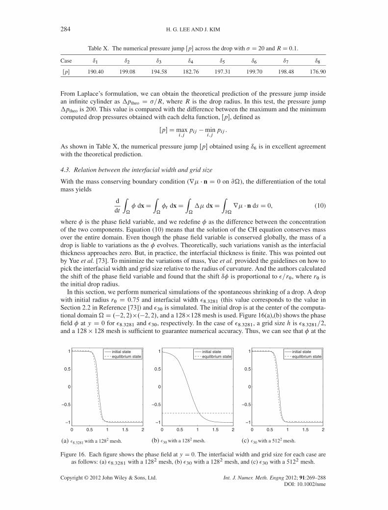
In this section, we perform numerical simulations of the spontaneous shrinking of a drop. A dropwith initial radius r0 D 0.75 and interfacial width �8.3281 (this value corresponds to the value inSection 2.2 in Reference [73]) and �30 is simulated. The initial drop is at the center of the computa-tional domain�D .�2, 2/�.�2, 2/, and a 128�128mesh is used. Figure 16(a),(b) shows the phasefield � at y D 0 for �8.3281 and �30, respectively. In the case of �8.3281, a grid size h is �8.3281=2,and a 128 � 128 mesh is sufficient to guarantee numerical accuracy. Thus, we can see that � at the
0 0.5 1 1.5 2
−1
−0.5
0
0.5
1 initial stateequilibrium state
(a)
0 0.5 1 1.5 2
−1
−0.5
0
0.5
1 initial stateequilibrium state
0 0.5 1 1.5 2
−1
−0.5
0
0.5
1 initial stateequilibrium state
(b) (c)8.3281 with a 1282 mesh. 30 with a 1282 mesh. 30 with a 5122 mesh.
Figure 16. Each figure shows the phase field at y D 0. The interfacial width and grid size for each case areas follows: (a) �8.3281 with a 1282 mesh, (b) �30 with a 1282 mesh, and (c) �30 with a 5122 mesh.
Copyright © 2012 John Wiley & Sons, Ltd. Int. J. Numer. Meth. Engng 2012; 91:269–288DOI: 10.1002/nme
DELTA FUNCTIONS FOR PHASE FIELD MODELS 285
Test1 Test1 Test2 Test3 Test4 Test5 Test5 Test50
10
20
30
40
50
60
70
δ3
δ4
δ6
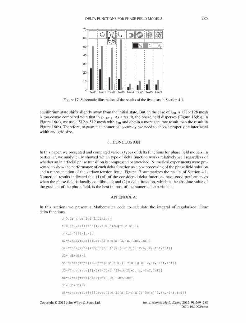
Figure 17. Schematic illustration of the results of the five tests in Section 4.1.
equilibrium state shifts slightly away from the initial state. But, in the case of �30, a 128�128 meshis too coarse compared with that in �8.3281. As a result, the phase field disperses (Figure 16(b)). InFigure 16(c), we use a 512� 512 mesh with �30 and obtain a more accurate result than the result inFigure 16(b). Therefore, to guarantee numerical accuracy, we need to choose properly an interfacialwidth and grid size.
5. CONCLUSION
In this paper, we presented and compared various types of delta functions for phase field models. Inparticular, we analytically showed which type of delta function works relatively well regardless ofwhether an interfacial phase transition is compressed or stretched. Numerical experiments were pre-sented to show the performance of each delta function as a postprocessing of the phase field solutionand a representation of the surface tension force. Figure 17 summarizes the results of Section 4.1.Numerical results indicated that (1) all of the considered delta functions have good performanceswhen the phase field is locally equilibrated; and (2) a delta function, which is the absolute value ofthe gradient of the phase field, is the best in most of the numerical experiments.
APPENDIX A:
In this section, we present a Mathematica code to calculate the integral of regularized Diracdelta functions.
Copyright © 2012 John Wiley & Sons, Ltd. Int. J. Numer. Meth. Engng 2012; 91:269–288DOI: 10.1002/nme
286 H. G. LEE AND J. KIM
ACKNOWLEDGEMENTS
This research was supported by Basic Science Research Program through the National Research Foundationof Korea (NRF), funded by the Ministry of Education, Science and Technology (No. 2011-0023794). Theauthors also wish to thank the reviewers for their constructive and helpful comments on the revision ofthis article.
REFERENCES
1. Rieger R, Weiss C, Wigley G, Bart H-J, Marr R. Investigating the process of liquid-liquid extraction by means ofcomputational fluid dynamics. Computers & Chemical Engineering 1996; 20:1467–1475.
2. West JL. Polymer-dispersed liquid crystals, Liquid-Crystalline Polymers Chap. 32, 1990.3. Tucker CL, Moldenaers P. Microstructural evolution in polymer blends. The Annual Review of Fluid Mechanics
2002; 34:177–210.4. Sundaresan S. Modeling the hydrodynamics of multiphase flow reactors: current status and challenges. AIChE
Journal 2000; 46:1102–1105.5. Crowe CT, Sommerfeld M, Tsuji Y. Multiphase Flows with Droplets and Particles. CRC Press: Florida, 1998.6. Dukowicz JK. A particle-fluid numerical model for liquid sprays. Journal of Computational Physics 1980;
35:229–253.7. Ménétrier-Deremblem L, Tabeling P. Droplet breakup in microfluidic junctions of arbitrary angles. Physical Review
E 2006; 74:035303-1–035303-4.8. De Menech M. Modeling of droplet breakup in a microfluidic T-shaped junction with a phase-field model. Physical
Review E 2006; 73:031505-1–031505-9.9. Tryggvason G, Bunner B, Esmaeeli A, Juric D, Al-Rawahi N, Tauber W, Han J, Nas S, Jan Y-J. A front-tracking
method for the computations of multiphase flow. Journal of Computational Physics 2001; 169:708–759.10. Unverdi SO, Tryggvason G. A front-tracking method for viscous, incompressible, multi-fluid flows. Journal of
Computational Physics 1992; 100:25–37.11. Pederzani J, Haj-Hariri H. A numerical method for the analysis of flexible bodies in unsteady viscous flows.
International Journal for Numerical Methods in Engineering 2006; 68:1096–1112.12. Udaykumar HS, Kan H-C, Shyy W, Tran-Son-Tay R. Multiphase dynamics in arbitrary geometries on fixed cartesian
grids. Journal of Computational Physics 1997; 137:366–405.13. Kietzmann CvL, Van Der Walt JP, Morsi YS. A free-front tracking algorithm for a control-volume-based Hele-Shaw
method. International Journal for Numerical Methods in Engineering 1998; 41:253–269.14. Mehdi-Nejad V, Mostaghimi J, Chandra S. Modelling heat transfer in two-fluid interfacial flows. International
Journal for Numerical Methods in Engineering 2004; 61:1028–1048.15. Battaglia L, Storti MA, D’Elia J. Bounded renormalization with continuous penalization for level set interface-
capturing methods. International Journal for Numerical Methods in Engineering 2010; 84:830–848.16. Challis VJ, Guest JK. Level set topology optimization of fluids in Stokes flow. International Journal for Numerical
Methods in Engineering 2009; 79:1284–1308.17. Gómez P, Hernández J, López J. On the reinitialization procedure in a narrow-band locally refined level set method
for interfacial flows. International Journal for Numerical Methods in Engineering 2005; 63:1478–1512.18. Sochnikov V, Efrima S. Level set calculations of the evolution of boundaries on a dynamically adaptive grid.
International Journal for Numerical Methods in Engineering 2003; 56:1913–1929.19. Kim J. A continuous surface tension force formulation for diffuse-interface models. Journal of Computational
Physics 2005; 204:784–804.20. Kim J. Phase field computations for ternary fluid flows. Computer Methods in Applied Mechanics and Engineering
2007; 196:4779–4788.21. Kim J. A generalized continuous surface tension force formulation for phase-field models for multi-component
immiscible fluid flows. Computer Methods in Applied Mechanics and Engineering 2009; 198:3105–3112.22. Yue P, Feng JJ, Liu C, Shen J. A diffuse-interface method for simulating two-phase flows of complex fluids.
The Journal of Fluid Mechanics 2004; 515:293–317.23. Griffith BE, Hornung RD, McQueen DM, Peskin CS. An adaptive, formally second order accurate version of the
immersed boundary method. Journal of Computational Physics 2007; 223:10–49.24. Griffith BE, Peskin CS. On the order of accuracy of the immersed boundary method: Higher order convergence rates
for sufficiently smooth problems. Journal of Computational Physics 2005; 208:75–105.25. LeVeque RJ, Li Z. The immersed interface method for elliptic equations with discontinuous coefficients and singular
sources. SIAM Journal on Numerical Analysis 1994; 31:1019–1044.26. Peskin CS. The immersed boundary method. Acta Numerica 2002; 11:479–517.27. Roma AM, Peskin CS, Berger MJ. An adaptive version of the immersed boundary method. Journal of Computational
Physics 1999; 153:509–534.28. Shin SJ, Huang W-X, Sung HJ. Assessment of regularized delta functions and feedback forcing schemes for an
immersed boundary method. International Journal for Numerical Methods in Fluids 2008; 58:263–286.29. Stockie JM. Analysis and computation of immersed boundaries, with application to pulp fibres. Ph.D. thesis, Institute
of Applied Mathematics, University of British Columbia, 1997.
Copyright © 2012 John Wiley & Sons, Ltd. Int. J. Numer. Meth. Engng 2012; 91:269–288DOI: 10.1002/nme
DELTA FUNCTIONS FOR PHASE FIELD MODELS 287
30. Yang X, Zhang X, Li Z, He G-W. A smoothing technique for discrete delta functions with application to immersedboundary method in moving boundary simulations. Journal of Computational Physics 2009; 228:7821–7836.
31. Chen L, Li Y. A numerical method for two-phase flows with an interface. Environmental Modelling & Software1998; 13:247–255.
32. Coward AV, Renardy YY, Renardy M, Richards JR. Temporal evolution of periodic disturbances in two-layerCouette flow. Journal of Computational Physics 1997; 132:346–361.
33. Gao D, Morley NB, Dhir V. Numerical simulation of wavy falling film flow using VOF method. Journal ofComputational Physics 2003; 192:624–642.
34. Gueyffier D, Li J, Nadim A, Scardovelli R, Zaleski S. Volume-of-fluid interface tracking with smoothed surfacestress methods for three-dimensional flows. Journal of Computational Physics 1999; 152:423–456.
35. Lafaurie B, Nardone C, Scardovelli R, Zaleski S, Zanetti G. Modelling merging and fragmentation in multiphaseflows with SURFER. Journal of Computational Physics 1994; 113:134–147.
36. Lörstad D, Fuchs L. High-order surface tension VOF-model for 3D bubble flows with high density ratio. Journal ofComputational Physics 2004; 200:153–176.
37. Meier M, Yadigaroglu G, Smith BL. A novel technique for including surface tension in PLIC-VOF methods.European Journal of Mechanics - B/Fluids 2002; 21:61–73.
38. Rudman M. A volume-tracking method for incompressible multifluid flows with large density variations. Interna-tional Journal for Numerical Methods in Fluids 1998; 28:357–378.
39. Scardovelli R, Zaleski S. Direct numerical simulation of free-surface and interfacial flow. The Annual Review ofFluid Mechanics 1999; 31:567–603.
40. Tang H, Wrobel LC, Fan Z. Tracking of immiscible interfaces in multiple-material mixing processes. ComputationalMaterials Science 2004; 29:103–118.
41. Engquist B, Tornberg A-K, Tsai R. Discretization of dirac delta functions in level set methods. Journal ofComputational Physics 2005; 207:28–51.
42. Jin S, Wen X. Hamiltonian-preserving schemes for the Liouville equation with discontinuous potentials. Communi-cations in Mathematical Sciences 2005; 3:285–315.
43. Jin S, Liu H, Osher S, Tsai Y-HR. Computing multivalued physical observables for the semiclassical limit of theSchrödinger equation. Journal of Computational Physics 2005; 205:222–241.
44. Jin S, Liu H, Osher S, Tsai Y-HR. Computing multi-valued physical observables for high frequency limit ofsymmetric hyperbolic systems. Journal of Computational Physics 2005; 210:497–518.
45. Smereka P. The numerical approximation of a delta function with application to level set methods. Journal ofComputational Physics 2006; 211:77–90.
46. Sussman M, Smereka P, Osher S. A level set method for computing solutions to incompressible two-phase flow.Journal of Computational Physics 1994; 114:146–159.
47. Towers JD. Two methods for discretizing a delta function supported on a level set. Journal of Computational Physics2007; 220:915–931.
48. Wen X. High order numerical methods to a type of delta function integrals. Journal of Computational Physics 2007;226:1952–1967.
49. Cahn JW. On spinodal decomposition. Acta Metallurgica 1961; 9:795–801.50. Cahn JW, Hilliard JE. Free energy of a nonuniform system. I. Interfacial free energy. Journal of Chemical Physics
1958; 28:258–267.51. Eyre D J. An Unconditionally Stable One-Step Scheme for Gradient Systems. http://www.math.utah.edu/~eyre/
research/methods/stable.ps.52. Eyre DJ. Computational and Mathematical Models of Microstructural Evolution. The Material Research Society:
Pennsylvania, 1998.53. Kim J, Bae H-O. An unconditionally stable adaptive mesh refinement for Cahn–Hilliard equation. Journal of the
Korean Physical Society 2008; 53:672–679.54. Vollmayr-Lee BP, Rutenberg AD. Fast and accurate coarsening simulation with an unconditionally stable time step.
Physical Review E 2003; 68:066703-1–066703-13.55. Kim J. A numerical method for the Cahn–Hilliard equation with a variable mobility. Communications in Nonlinear
Science and Numerical Simulation 2007; 12:1560–1571.56. Hirt CW, Nichols BD. Volume of fluid (VOF) method for the dynamics of free boundaries. Journal of Computational
Physics 1981; 39:201–225.57. Brackbill JU, Kothe DB, Zemach C. A continuum method for modelling surface tension. Journal of Computational
Physics 1992; 100:335–354.58. Badalassi VE, Ceniceros HD. BanerjeeS. Computation of multiphase systems with phase field models. Journal of
Computational Physics 2003; 190:371–397.59. Chang YC, Hou TY, Merriman B, Osher S. A level set formulation of Eulerian interface capturing methods for
incompressible fluid flows. Journal of Computational Physics 1996; 124:449–464.60. Chella R. Mixing of a two-phase fluid by cavity flow. Physical Review E 1996; 53:3832–3840.61. Renardy YY, Renardy M, Cristini V. A new volume-of-fluid formation for surfactants and simulations of drop
deformation under shear at a low viscosity ratio. European Journal of Mechanics - B/Fluids 2002; 21:49–59.62. Khismatullin D, Renardy YY, Renardy M. Development and implementation of VOF-PROST for 3D viscoelastic
liquid. liquid simulations. Journal of Non-Newtonian Fluid Mechanics 2006; 140:120–131.
Copyright © 2012 John Wiley & Sons, Ltd. Int. J. Numer. Meth. Engng 2012; 91:269–288DOI: 10.1002/nme
288 H. G. LEE AND J. KIM
63. Pilliod Jr. JE, Puckett EG. Second-order volume-of-fluid algorithms for tracking material interfaces. Journal ofComputational Physics 2004; 199:465–502.
64. Renardy YY, Renardy M. PROST: a parabolic reconstruction of surface tension for the volume-of-fluid method.Journal of Computational Physics 2002; 183:400–421.
65. Osher S, Sethian J. Fronts propagating with curvature-dependent speed: algorithms based on Hamilton-Jacobiformulations. Journal of Computational Physics 1988; 79:12–49.
66. Hou TY, Li Z, Osher S, Zhao H. A hybrid method for moving interface problems with application to the Hele-Shawflow. Journal of Computational Physics 1997; 134:236–252.
67. Liu X-D, Fedkiw RP, Kang M. A boundary condition capturing method for Poisson’s equation on irregular domains.Journal of Computational Physics 2000; 160:151–178.
68. Peng D, Merriman B, Osher S, Zhao H, Kang M. A PDE-based fast local level set method. Journal of ComputationalPhysics 1990; 155:410–438.
69. Tornberg A-K, Engquist B. Numerical approximations of singular source terms in differential equations. Journal ofComputational Physics 2004; 200:462–488.
70. Towers JD. Finite difference methods for approximating Heaviside functions. Journal of Computational Physics2009; 228:3478–3489.
71. Yang S-D, Lee HG, Kim J. A phase-field approach for minimizing the area of triply periodic surfaces with volumeconstraint. Computer Physics Communications 2010; 181:1037–1046.
72. Wang X. Phase field models and simulations of vesicle bio-membranes. Ph.D. thesis, Department of Mathematics,Penn State University, 2005.
73. Yue P, Zhou C, Feng JJ. Spontaneous shrinkage of drops and mass conservation in phase-field simulations. Journalof Computational Physics 2007; 223:1–9.
74. Jacqmin D. Contact-line dynamics of a diffuse fluid interface. The Journal of Fluid Mechanics 2000; 402:57–88.75. Rayleigh L. Investigation of the character of the equilibrium of an incompressible heavy fluid of variable density.
Proceedings of the London Mathematical Society 1883; 14:170–177.76. Taylor G. The instability of liquid surfaces when accelerated in a direction perpendicular to their planes. I.
Proceedings of the Royal Society of London A 1950; 201:192–196.77. Lee HG, Kim K, Kim J. On the long time simulation of the Rayleigh–Taylor instability. International Journal for
Numerical Methods in Engineering 2011; 85:1633–1647.78. LeVeque R. High-resolution conservative algorithms for advection in incompressible flow. SIAM Journal on
Numerical Analysis 1996; 33:627–665.79. Enright D, Fedkiw R, Ferziger J, Mitchell I. A hybrid particle level set method for improved interface capturing.
Journal of Computational Physics 2002; 183:83–116.80. Hyde S, Andersson S, Larsson K, Blum Z, Landh T, Lidin S, Ninham BW. The Language of Shape: The Role of
Curvature in Condensed Matter: Physics, Chemistry and Biology. Elsevier Science: Amsterdam, 1997.81. Rajagopalan S, Robb RA. Schwarz meets Schwann: design and fabrication of biomorphic and durataxic tissue
engineering scaffolds. Medical Image Analysis 2006; 10:693–712.82. Von Schnering HG, Nesper R. Nodal surfaces of Fourier series: fundamental invariants of structured matter.
Zeitschrift für Physik B Condensed Matter 1991; 83:407–412.83. Jung Y, Chu KT, Torquato S. A variational level set approach for surface area minimization of triply-periodic
surfaces. Journal of Computational Physics 2007; 223:711–730.84. Rider WJ, Kothe D. Reconstructing volume tracking. Journal of Computational Physics 1998; 141:112–152.85. Ganesan S, Matthies G, Tobiska L. On spurious velocities in incompressible flow problems with interfaces. Computer
Methods in Applied Mechanics and Engineering 2007; 196:1193–1202.86. Gerbeau J-F, Le Bris C, Bercovier M. Spurious velocities in the steady flow of an incompressible fluid subjected to
external forces. International Journal for Numerical Methods in Fluids 1997; 25:679–695.87. Gresho P, Lee R, Chan S, Leone JA. A new finite element for incompressible or Boussinesq fluids. Proceedings of
the Third International Conference on Finite Elements in Flow Problems, Banff, Canada, 1980.88. Pelletier D, Fortin A, Camarero R. Are FEM solutions of incompressible flows really incompressible? (Or how
simple flows can cause headaches!). International Journal for Numerical Methods in Fluids 1989; 9:99–112.
Copyright © 2012 John Wiley & Sons, Ltd. Int. J. Numer. Meth. Engng 2012; 91:269–288DOI: 10.1002/nme


![A Helmholtz’ Theorem€¦ · B The Dirac Delta Function B.1 The One-Dimensional Dirac Delta Function The Dirac delta function [1] in one-dimensional space may be defined by the](https://img.pdfslide.net/doc/110x75/5fe40cfa3aac814e62636cef/a-helmholtza-theorem-b-the-dirac-delta-function-b1-the-one-dimensional-dirac.jpg)


![A CAUCHY–DIRAC DELTA FUNCTION - arXiv · But did Dirac introduce the delta function? Laugwitz [52, p. 219] notes that probably the first appearance of the (Dirac) delta function](https://img.pdfslide.net/doc/110x75/5ac33aab7f8b9a220b8b8e19/a-cauchydirac-delta-function-arxiv-did-dirac-introduce-the-delta-function.jpg)