Embed Size (px)
Citation preview
The Office of Financial Research (OFR) Working Paper Series allows members of the OFR staff and their coauthors to disseminate preliminary research findings in a format intended to generate discussion and critical comments. Papers in the OFR Working Paper Series are works in progress and subject to revision. Views and opinions expressed are those of the authors and do not necessarily represent official positions or policy of the OFR or Treasury. Comments and suggestions for improvements are welcome and should be directed to the authors. OFR working papers may be quoted without additional permission.
Regulatory Arbitrage in Repo Markets
Benjamin Munyan Office of Financial Research and Vanderbilt University [email protected]
15-22 | October 29, 2015
Regulatory Arbitrage in Repo Markets∗
Benjamin Munyan†
October 29, 2015
Abstract
Non-U.S. banks with relatively low capital ratios appear to temporarily remove anaverage of $170 billion from the U.S. market for tri-party repurchase agreements (repo)before each quarter-end in order to appear safer and less levered. This amount is morethan double the $76 billion market-wide drop in tri-party repo during the turmoil ofthe 2008 financial crisis and represents about 10% of the entire tri-party repo market.Such window dressing-induced deleveraging spills over into agency bond markets andmoney market funds and affects market liquidity each quarter.
∗The views expressed in this paper are solely those of the author and do not necessarily reflect the positionof the Office of Financial Research (OFR), the U.S. Department of the Treasury, the U.S. Securities and Ex-change Commission, the Financial Industry Regulatory Authority, the Federal Reserve Board of Governors,or the Federal Reserve Bank of New York. This paper uses confidential tri-party repo data to study marketactivity but does not reveal identities or positions of individual market participants.Special thanks to my dissertation committee: Pete Kyle, Russ Wermers, Mark Loewenstein, and Rich
Mathews. In addition this paper has benefited tremendously from valuable comments and conversations withMeraj Allahrahka, Viktoria Baklanova, Gurdip Bakshi, Jill Cetina, Jonathan Cohn, Adam Copeland, MichaelFaulkender, Greg Feldberg, Kathleen Hanley, Antoine Martin, Matthew McCormick, Patricia Mosser, Al-berto Rossi, Srihari Santosh, Anjan Thakor, Haluk Unal, Yajun Wang, and Peyton Young. I would also liketo thank Joe Bishop, Matt Earley, Regina Fuentes, Brook Herlach, Alicia Marshall, Matthew Reed, JulieVorman, and Valerie Wells for their help and support of this research. All remaining errors are mine.†Vanderbilt University, Owen Graduate School of Management; and the Office of Financial Research,
U.S. Department of the Treasury. E-mail: [email protected]
Introduction
I investigate the stability and composition of the repurchase agreement (repo) market and
how window dressing creates spillovers and affects systemic risk. Window dressing is the
practice in which financial institutions adjust their activity around an anticipated period
of oversight or public disclosure to appear safer or more profitable to outside monitors.
The repo market is a form of securitized banking that provides critical overnight funding
for the financial system but is vulnerable to runs. Several studies have suggested that
instability in the repo market—whether through a margin spiral effect in bilateral repo or
a run on individual institutions by their repo lenders in tri-party—helped cause the 2008
financial crisis.12 Its short-term nature means the repo market can also accommodate window
dressing, or temporary adjustments around a reporting period. However, like most two-sided
markets, it is difficult for outsiders to identify whether a change in repo market activity is
due to window dressing or rather to normal changes in the underlying supply and demand
of that market. I combine data sources for both supply and demand factors in the repo
market to overcome this problem and show that a type of repo market window dressing has
continued to occur among non-U.S. bank dealers each quarter since the 2008 financial crisis,
and this window dressing creates spillover effects in other markets.
My primary data source is confidential regulatory reports on daily tri-party repo trans-
action summaries since July 2008, obtained from the Federal Reserve Board of Governors
(Federal Reserve) and the U.S. Treasury Office of Financial Research. Tri-party repo is the
ultimate source of cash financing for many other repo transactions, and by extension much1See for example Gorton and Metrick (2012), Krishnamurthy, Nagel, and Orlov (2014), Copeland, Martin,
and Walker (2011), Martin, Skeie, and von Thadden (2014), and Ivashina and Scharfstein (2010).2The window dressing described in this paper is different from the “Repo 105” program that Lehman
Brothers used in 2008 to hide its actual leverage. In that program, Lehman accepted a relatively high 5%haircut in order to count its repo transactions as “true sales,” allowing it to significantly reduce its reportedleverage, even though it remained under a contractual obligation to repurchase those assets. In contrast, thenon-U.S. dealers whose activities are described in this paper appear to be selling assets before the quarter-end and then re-acquiring them after .I find no evidence that they are simply raising haircuts and, althoughthey tend to re-acquire those assets once a new quarter starts, I do not discover any obligation on their partto do so.
1
of the shadow banking system. This dataset covers the entire $1.7 trillion tri-party repo
market, includes details on how much a dealer (a “cash borrower”) borrows using each type
of collateral, and shows how costly it is for the dealer to borrow each day. It also includes
data starting from January 2011 on the network of daily repo borrowing between dealers
and the various institutions that are their repo counterparties (“cash lenders”). In a time
series regression controlling for dealers’ home regions, I show that broker-dealer subsidiaries
of non-U.S. banks use repo to window-dress roughly $170 billion of assets each quarter, in
what appears to be a form of regulatory arbitrage.
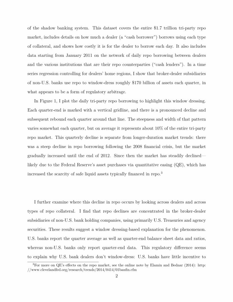
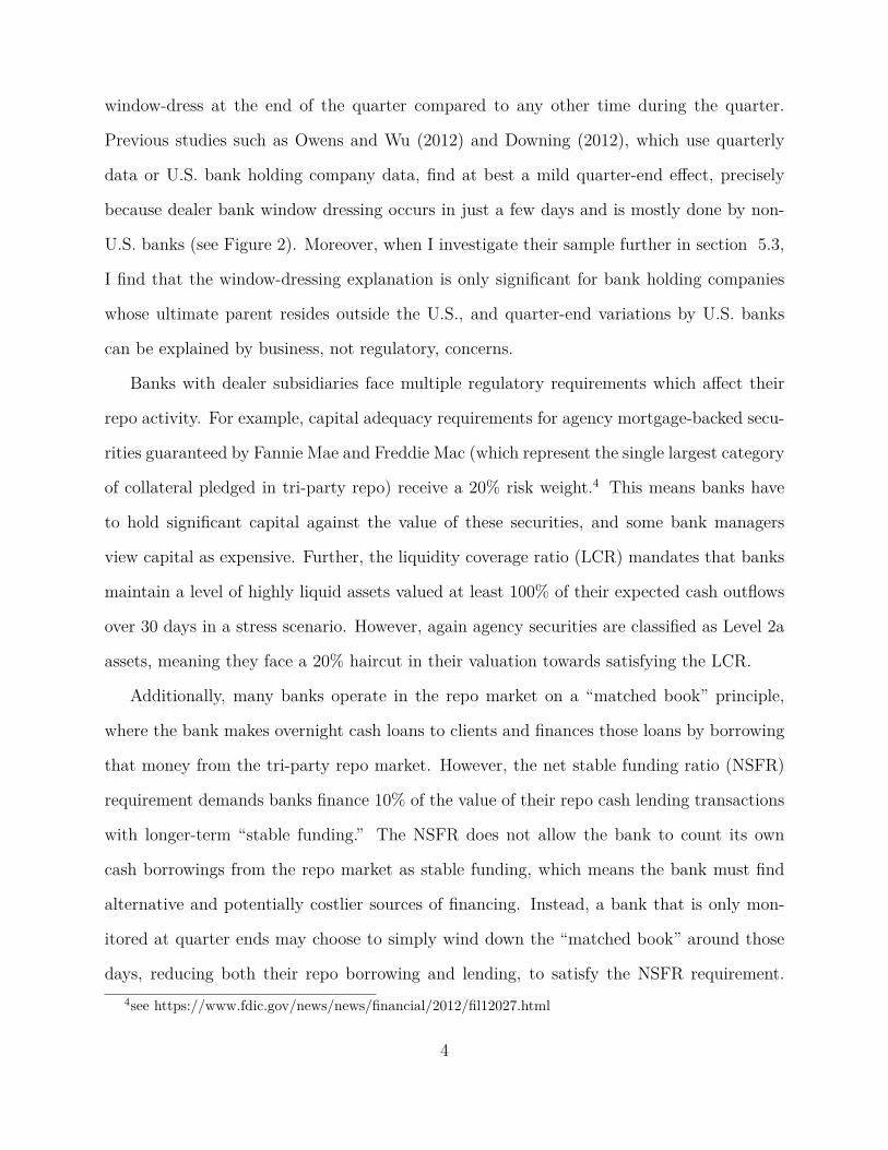
In Figure 1, I plot the daily tri-party repo borrowing to highlight this window dressing.
Each quarter-end is marked with a vertical gridline, and there is a pronounced decline and
subsequent rebound each quarter around that line. The steepness and width of that pattern
varies somewhat each quarter, but on average it represents about 10% of the entire tri-party
repo market. This quarterly decline is separate from longer-duration market trends: there
was a steep decline in repo borrowing following the 2008 financial crisis, but the market
gradually increased until the end of 2012. Since then the market has steadily declined—
likely due to the Federal Reserve’s asset purchases via quantitative easing (QE), which has
increased the scarcity of safe liquid assets typically financed in repo.3
I further examine where this decline in repo occurs by looking across dealers and across
types of repo collateral. I find that repo declines are concentrated in the broker-dealer
subsidiaries of non-U.S. bank holding companies, using primarily U.S. Treasuries and agency
securities. These results suggest a window dressing-based explanation for the phenomenon.
U.S. banks report the quarter average as well as quarter-end balance sheet data and ratios,
whereas non-U.S. banks only report quarter-end data. This regulatory difference seems
to explain why U.S. bank dealers don’t window-dress: U.S. banks have little incentive to3For more on QE’s effects on the repo market, see the online note by Elamin and Bednar (2014): http:
//www.clevelandfed.org/research/trends/2014/0414/01banfin.cfm2
Figure 1. Daily Tri-Party Repo Outstanding
Notes: The vertical axis represents the value in trillions of dollars of collateral outstanding pledged in repoeach day from July 1, 2008 to July 31, 2014. Quarter-ends are marked with vertical dashed lines, andyear-ends are marked with heavier dash-dotted lines. I exclude repo borrowing by the Federal Reserve Bankof New York, and I exclude the dates of 7/17/2008 and 4/11/2013 because of missing data from one of theclearing banks.Source: Federal Reserve Board of Governors
3
window-dress at the end of the quarter compared to any other time during the quarter.
Previous studies such as Owens and Wu (2012) and Downing (2012), which use quarterly
data or U.S. bank holding company data, find at best a mild quarter-end effect, precisely
because dealer bank window dressing occurs in just a few days and is mostly done by non-
U.S. banks (see Figure 2). Moreover, when I investigate their sample further in section 5.3,
I find that the window-dressing explanation is only significant for bank holding companies
whose ultimate parent resides outside the U.S., and quarter-end variations by U.S. banks
can be explained by business, not regulatory, concerns.
Banks with dealer subsidiaries face multiple regulatory requirements which affect their
repo activity. For example, capital adequacy requirements for agency mortgage-backed secu-
rities guaranteed by Fannie Mae and Freddie Mac (which represent the single largest category
of collateral pledged in tri-party repo) receive a 20% risk weight.4 This means banks have
to hold significant capital against the value of these securities, and some bank managers
view capital as expensive. Further, the liquidity coverage ratio (LCR) mandates that banks
maintain a level of highly liquid assets valued at least 100% of their expected cash outflows
over 30 days in a stress scenario. However, again agency securities are classified as Level 2a
assets, meaning they face a 20% haircut in their valuation towards satisfying the LCR.
Additionally, many banks operate in the repo market on a “matched book” principle,
where the bank makes overnight cash loans to clients and finances those loans by borrowing
that money from the tri-party repo market. However, the net stable funding ratio (NSFR)
requirement demands banks finance 10% of the value of their repo cash lending transactions
with longer-term “stable funding.” The NSFR does not allow the bank to count its own
cash borrowings from the repo market as stable funding, which means the bank must find
alternative and potentially costlier sources of financing. Instead, a bank that is only mon-
itored at quarter ends may choose to simply wind down the “matched book” around those
days, reducing both their repo borrowing and lending, to satisfy the NSFR requirement.4see https://www.fdic.gov/news/news/financial/2012/fil12027.html
4
This is problematic because the NSFR was designed to prevent a contagion scenario in the
dealer system, where dealers lose unstable funding sources in a crisis and are forced to with-
draw credit to their clients. During the interim period between monitoring, a bank may be
operating above the NSFR and reducing the effectiveness of these regulatory safeguards.
I establish that the decline in repo is caused by the non-U.S. bank dealers—not their
repo lenders—by combining this data with reports on money market mutual fund portfolio
holdings and assets under management from iMoneyNet and the U.S. Securities and Ex-
change Commission (SEC) form N-MFP, and quarterly bank parent balance sheet data from
Bankscope. I then perform a joint estimation of supply and demand in the repo market
and find that a non-U.S. dealer’s quarter-end window dressing is strongly predicted by its
leverage the prior quarter. To further identify causality, I use network data of repo fund-
ing between dealers and cash lenders to perform a within-lender regression that controls for
potential omitted cash supply factors.
I show significant spillover effects from repo window dressing to other markets. If non-U.S.
bank dealers window-dress to report lower leverage, then when they withdraw collateral from
repo, they must also sell those assets. I use the Financial Industry Regulatory Authority’s
(FINRA) Trade Reporting and Compliance Engine (TRACE) Agency bond transaction-level
data from 2010 to 2013 in a time series regression with time-fixed effects for each quarter5
to test whether dealers are trading abnormally around the end of the quarter. I find that
dealers sell heavily to customers in the last days of the quarter and immediately buy agency
bonds back once the new quarter starts. In an empirical test of the theoretical findings of
Froot and Stein (1998), I find that this self-imposed deleveraging causes a significant change
in the market quality for agency bonds at quarter-end.
At the same time, declines in repo borrowing due to window dressing leave cash lenders5Because the days around a quarter-end will span two quarters, and because there is a pronounced
downward trend in the overall repo market over my sample, there may be concern that using quarter fixedeffects will bias the estimates for repo borrowing at the end of an old quarter and the start of a new one awayfrom each other, overstating this window dressing result as an artifact of my methodology. As a robustnesstest, I have estimated these results with year fixed effects and by shifting the fixed effects reference 1 monthforward, as well as without any fixed effects at all, and the results persist in both magnitude and significance.
5
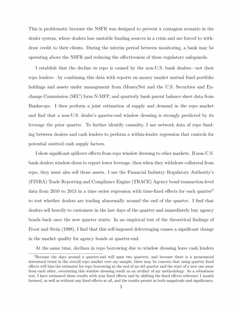
Figure 2. Repo Borrowing at the End of an Average Quarter
(Top left): I include a copy of Figure 1, with trillions of dollars in daily repo borrowing, as a reference.(Top right): This figure represents the average daily repo outstanding over the course of a single quarter.The average quarter has 62 trading days, and I position the end of the quarter (marked by a vertical line)in the middle of the figure to highlight the quarter-end decline and subsequent rebound of repo borrowing.The vertical axis again represents the market value of collateral in trillions of dollars.(Bottom left): I separate the average repo outstanding over a single quarter by type of asset. The solid blueline uses the left axis and represents average repo borrowing backed by the safest collateral: U.S. Treasuries,agency debentures, and agency mortgage-backed securities, and agency collateralized mortgage obligations.The dotted red line uses the right axis and represents average repo borrowing backed by all other types ofcollateral. Both axes are in trillions of dollars.(Bottom right): Here I present the average repo outstanding over a single quarter separated by the region ofthe repo cash borrower (i.e., the dealer that is pledging collateral in the repo). The left and right axes areboth in billions of dollars. I exclude non-bank dealers from this subplot. The dotted green line representsrepo borrowing by U.S. bank dealers and can also be distinguished by its distinct behavior: this line touchesthe left axis at roughly $780 billion and does not dip as markedly as the other two lines at the end of thequarter. The solid blue line represents repo borrowing by European bank dealers. Both U.S. and Europeanbank dealer repo borrowing are in reference to the left axis. The dashed red line shows Japanese bank dealerrepo borrowing, and because Japanese bank dealers are a much smaller segment of the repo market, I plottheir line using the right axis.Enlarged individual copies of these figures are included in the appendix.Source: Federal Reserve Board of Governors
6
such as money market mutual funds with excess cash that they struggle to invest. My
analysis of monthly money market fund (MMF) portfolios shows that despite being able to
anticipate window dressing, MMFs are still unable to find any investment at all for about
$20 billion of cash each quarter-end before September 2013. The Federal Reserve’s reverse
repurchase agreement (RRP) program began at that time with the stated intention of being
a tool for raising interest rates, but it has become a substitute investment for repo lenders
during times of window dressing.
Section 1 of this paper reviews the current state of the literature, and how my findings
contribute to an understanding of repo markets and their potential for systemic risk and
to the literature on seasonality. Section 2 provides an overview of the repo markets and
the tri-party repo market’s important position relative to the bilateral and general collateral
repo markets. In section 3, I describe the datasets used in this paper, with a particular focus
on the regulatory tri-party repo data collection. Section 4 lays out my empirical strategy
to identify window dressing and establish dealers as the cause of it. I report the results of
robustness tests in Section 5. Section 6 shows how window dressing in repo markets has
necessary repercussions in at least two other markets: the market for agency bonds and the
money market mutual fund industry. Section 7 concludes with some policy recommendations
to prevent future window dressing, or at least mitigate its impact.
1 Literature Review
My paper contributes to existing literature focused on three main areas: the stability of
repo markets, seasonality (and its underlying causes), and the risk management of financial
intermediaries.
Since 2008, a surge has occurred in the literature that analyzes the role that repo mar-
kets played in the financial crisis. Gorton and Metrick (2009, 2012) suggest that haircuts
on collateral in bilateral repo created a destabilizing feedback effect, forcing cash borrowers
to delever by selling assets in a fire sale, which caused haircuts to rise even higher, precipi-7
tating the banking system’s insolvency. However Copeland, Martin, and Walker (2011) and
Krishnamurthy, Nagel, and Orlov (2014) find that in tri-party repo there is no spiral effect,
and the crisis in tri-party repo is more consistent with a run on certain dealers by their cash
lenders.
Difficult to determine in this discussion is the direction of causation for the effects these
papers describe. Indeed, Gorton and Metrick (2012) admit that “without a structural model
of repo markets, we are only able to talk about co-movement. . . thus we use the language
of ‘correlation’ rather than ‘causation’ in our empirical analysis.” Martin, Skeie, and von
Thadden (2014) present a theoretical model of repo lending that extends earlier bank run
models from Diamond and Dybvig (1983) and Qi (1994) to analyze runs on collateralized repo
borrowing instead of commercial bank deposits. The paper finds that liquidity constraints
(the size, short-term leverage, and profitability of a repo borrower), as well as collateral
constraints (the value to lenders from taking ownership of repo collateral directly, the pro-
ductivity of a borrower from continuing to manage collateral, as well as borrower size and
short-term leverage) determine a repo borrower’s ability to survive a crisis. However, their
model also predicts that outside of a crisis, each borrower invests (and borrows) as much as
possible.
In this paper I provide evidence that the quarterly decline in repo is not due to a run-type
panic, but rather due to repo becoming relatively less profitable at quarter-end for non-U.S.
bank dealers. This is consistent with Martin, Skeie, and von Thadden (2014), who suggest
that dealers will adjust their repo borrowing to trade off between profitability and liquidity
risk constraints. When repo is more profitable, their paper suggests dealers will take more
liquidity risk in the quantity and type of collateral they pledge, increasing their exposure
to the risk of a run by their cash lenders. Therefore, if there is a shock to collateral again
in the future (like the 2007 asset-backed commercial paper crisis), non-U.S. bank tri-party
borrowers may be the ones more vulnerable to a run.
This paper adds to extensive literature on seasonality. Since January effects were docu-
8
mented by Rozeff and Kinney (1976) and Keim (1983), researchers have tried to find under-
lying explanations for the effect. Ritter (1988) looks at the behavior of investors around the
turn of the year and finds individual investors may drive the January effect. Constantinides
(1984), Sias and Starks (1997), and Poterba and Weisbenner (2001) look more deeply and
find that underlying tax reasons might drive investors’ year-end abnormal trading.
Other papers suggest window dressing may explain seasonal effects. Haugen and Lakon-
ishok (1987) suggest the January effect might be explained by fund managers adjusting their
portfolios to appear safer for their end-of-year filings. Lakonishok et al. (1991) investigate
pension fund managers and find they sell losers in the fourth quarter to make it appear that
they are good at picking stocks. In a sample of banks from 1978 to 1986, Allen and Saunders
(1992) claim to find upward window dressing, in which banks increase their balance sheet
each quarter to appear larger. Musto (1997) finds further support for this by examining
the difference in trading behavior of commercial paper and Treasury bills around the year-
end, and suggests that intermediaries don’t want to show a risky portfolio to regulators or
investors. However, Wermers (1999) finds no evidence of window dressing by mutual fund
managers at the end of the year versus other quarters. In contrast, I do not see much evi-
dence of January effects in repo, but I do find support for window dressing at the quarterly
frequency, which spills over into fixed income markets.
In the repo market specifically, the literature has looked for evidence of window dressing
or a liquidity habitat preference. So far the results for window dressing have been mixed.
Owens and Wu (2012) and Downing (2012) look at U.S. bank repo behavior at the end of the
quarter versus quarter average repo borrowing, and find that banks window-dress modestly
at the end of the quarter. However, they are unable to definitively claim that they find
window dressing and not just a shift in banks’ funding sources. In section 5, I show that
controlling for the country of a bank dealer is critical to interpreting their results.
Non-U.S. banks were outside the scope of those previous studies, but it is precisely
among non-U.S. bank dealers that I find significant window dressing. U.S. banks report
9
the quarter-average as well as quarter-end balance sheet data and ratios, whereas non-U.S.
banks only report quarter-end data. This regulatory difference may help explain why U.S.
bank dealers don’t window-dress: U.S. banks have little incentive to window-dress at the end
of the quarter compared to any other time during the quarter. Other institutional features,
or differences in the regulatory environment inside and outside the U.S. may also contribute
to a dealer’s decision to window-dress, however, differential monitoring seems likely to be a
primary factor.
A series of papers by Griffiths andWinters (1997, 2005) and Kotomin, Smith, andWinters
(2008) propose that window dressing does not occur in repo, but, instead, repo declines are
driven by a preferred liquidity habitat model as in Modigliani and Sutch (1966). In this
scenario banks do not actively reduce their repo borrowing to hide leverage. Instead, cash
suppliers, such as money market funds, must cut their repo lending in order to redeem their
own investors’ outflows. In this paper I provide evidence from two data sources on money
market funds that show that money funds do not see outflows nearly as large as the drop in
repo outstanding, and, in fact, repo lenders have an excess of cash at the end of the quarter.
I further identify the quarterly decline as dealer-driven using a within-investor estimation
approach similar to that of Khwaja & Mian (2008), which uses time and investor-fixed effects
to control for unobserved demand factors.
Theoretical models by Froot, Scharfstein, and Stein (1993) and Froot and Stein (1998)
suggests that capital structure policy plays a critical role in risk management. A key im-
plication of their framework for financial intermediaries (including dealers) is that capital
adequacy constraints will generate asymmetric price effects in intermediated markets. When
dealers are capital-constrained, they will offer worse prices to trades that tighten capital con-
straints, and better prices to trades that relax those constraints. Empirical research by Naik
and Yadav (2003) uses daily detailed position data on each UK government bond dealer and
supports these conjectures.
Recent work by Koijen and Yogo (2013) finds that regulatory arbitrage by financial
10
intermediaries has real economic effects as well. Their study of U.S. life insurers shows
that risk transfers to off-balance-sheet and affiliated entities has the effect of reducing the
insurers’ risk-based capital, and increases their probability of default by a factor of 3.5.
Moreover, they estimate that eliminating this regulatory arbitrage would increase the life
insurance prices offered by those companies by 12%, and reduce the overall amount of U.S.
life insurance provided to households. Although these effects are much harder to detect
during the quarter among bank dealers, who can take risk through a diverse portfolio rather
than a single product like life insurance, I present evidence that dealer window dressing does
reduce market quality at the quarter-end when non-U.S. dealers are deleveraging.
2 Mechanics of the Repo Markets
This section provides a basic explanation of how a repurchase agreement works, the differ-
ences in the institutional operations of each of the three repo markets, and why tri-party
repo matters to the financial system. Readers who are already familiar with repo may wish
to skip ahead to Section 3.
A repurchase agreement (commonly shortened to “repo”) is a contract in which one party
sells securities with the agreement to repurchase those same securities at a specified maturity
date. The other party pays cash for those securities and promises to return them when the
repo matures and receive their cash plus interest, similar to a collateralized loan.
The second party (the cash lender) typically assigns a haircut to the cash amount they
pay, relative to the market value of securities received, as protection in case the first party
(the cash borrower) defaults and fails to return the cash. A repo is treated legally as a “true
sale,” which means the repo collateral is exempt from an automatic stay in bankruptcy
if the cash borrower defaults, and the cash lender can sell or hold the securities without
any encumbrance. However, many cash lenders will accept collateral that their charter or
prospectus would not permit them to hold directly—for example, money market mutual
funds (MMMFs) lending cash in repo against long-dated mortgage-backed securities (an-11
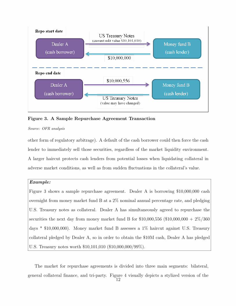
Figure 3. A Sample Repurchase Agreement Transaction
Source: OFR analysis
other form of regulatory arbitrage). A default of the cash borrower could then force the cash
lender to immediately sell those securities, regardless of the market liquidity environment.
A larger haircut protects cash lenders from potential losses when liquidating collateral in
adverse market conditions, as well as from sudden fluctuations in the collateral’s value.
Example:
Figure 3 shows a sample repurchase agreement. Dealer A is borrowing $10,000,000 cash
overnight from money market fund B at a 2% nominal annual percentage rate, and pledging
U.S. Treasury notes as collateral. Dealer A has simultaneously agreed to repurchase the
securities the next day from money market fund B for $10,000,556 ($10,000,000 + 2%/360
days * $10,000,000). Money market fund B assesses a 1% haircut against U.S. Treasury
collateral pledged by Dealer A, so in order to obtain the $10M cash, Dealer A has pledged
U.S. Treasury notes worth $10,101,010 ($10,000,000/99%).
The market for repurchase agreements is divided into three main segments: bilateral,
general collateral finance, and tri-party. Figure 4 visually depicts a stylized version of the12
flow of cash and collateral between participants in these different types of repo. In subsections
2.1 through 2.3, I offer more details about the key institutional differences and connections
between these markets.
2.1 Bilateral Repo Market
The bilateral repo market is unique in that its trades do not settle on the books of the two
large clearing banks—Bank of New York Mellon Corp. and JPMorgan Chase & Co. Instead,
bilateral repos (also called Delivery versus Payment repos) are negotiated and settled directly
between dealers and their clients. Dealers can act as either cash borrowers or cash lenders,
and their counterparties are primarily hedge funds and real estate investment trusts (REITs),
though banks and other institutions may participate to a smaller extent. The purpose of
bilateral is also distinct from tri-party and general collateral finance (GCF) repo: bilateral
repo is reportedly driven by market participants’ needs to acquire specific securities for
hedging or settlement purposes, not just to finance a portfolio. A recent study from the
Federal Reserve Bank of New York using primary dealer data estimates U.S. Treasuries
currently make up 90% of bilateral repo collateral.6 The estimated size of the bilateral repo
market varies: the Federal Reserve Bank of New York estimates the size of the bilateral repo
market at $1.4 trillion, on par with tri-party repo daily volume.
2.2 General Collateral Finance Repo Market
A general collateral finance (GCF) repo is an inter-dealer repo centrally cleared by the
Fixed Income Clearing Corporation (FICC) over Fedwire, in which the cash borrower and
cash lender directly negotiate a rate and duration for the repo, and specify a class of assets
(e.g., all mortgage-backed securities, or Treasuries with fewer than five years to maturity)6See note by Copeland, Davis, LeSueur, and Martin (2014): http://libertystreeteconomics.newyorkfed.
org/2014/07/lifting-the-veil-on-the-us-bilateral-repo-market.html .13
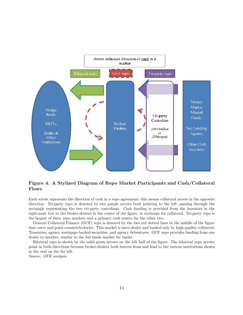
Figure 4. A Stylized Diagram of Repo Market Participants and Cash/CollateralFlows
Each arrow represents the direction of cash in a repo agreement; this means collateral moves in the oppositedirection. Tri-party repo is denoted by two purple arrows both pointing to the left, passing through therectangle representing the two tri-party custodians. Cash funding is provided from the investors in theright-most box to the broker-dealers in the center of the figure, in exchange for collateral. Tri-party repo isthe largest of three repo markets and a primary cash source for the other two.
General Collateral Finance (GCF) repo is denoted by the two red dotted lines in the middle of the figurethat curve and point counterclockwise. This market is inter-dealer and backed only by high-quality collateral:Treasuries, agency mortgage-backed securities, and agency debentures. GCF repo provides funding from onedealer to another, similar to the fed funds market for banks.
Bilateral repo is shown by the solid green arrows on the left half of the figure. The bilateral repo arrowspoint in both directions because broker-dealers both borrow from and lend to the various institutions shownin the oval on the far left.Source: OFR analysis
14
rather than specific securities, which can be pledged as collateral. GCF repos are unique
in that they have no haircut margin. The cash borrower can continue to use his or her
securities freely to make markets and clear trades that day until 11 a.m., when the cash
borrower must identify the specific securities it will actually deliver to the cash lender. GCF
repo was designed to improve inter-dealer liquidity by netting obligations through the FICC
and giving dealers flexibility to substitute collateral throughout the day as their portfolio
changes. In 2012 the GCF repo market’s total (pre-netting) average daily volume was $400
billion. However, since then the market has shrunk considerably, to only $210 billion per
day in June 2014.7
2.3 Tri-party Repo Market
The tri-party repo market gets its name from the manner in which transactions are cleared.
Tri-party repo counterparties transact through one of two custodian banks: Bank of New
York Mellon and JPMorgan Chase. These two custodians provide tools to value collateral
and apply haircuts for cash lenders, and help cash borrowers allocate their portfolio across
lenders to achieve the lowest cost of financing. Collateral is moved from a cash borrower’s
account with the custodian to the cash lender’s account with the custodian in exchange for
cash at the start of a repo, and the transaction is reversed the next morning when the repo
is unwound.8
The tri-party repo market finances approximately $1.7 trillion of collateral each day.
There are 14 broad classes of collateral accepted, but over 80% of repos are backed by the
most liquid assets: U.S. Treasuries or agency-backed securities. There are 63 different deal-
ers, who get their cash funding from 170 different cash lenders (aggregating all subsidiaries
to the parent level). Most cash lenders are either money market mutual funds (MMMFs), or7Source: DTCC: http://www.dtcc.com/charts/dtcc-gcf-repo-index.aspx .8In a term repo, this daily unwind still occurs, meaning the custodian extends an intraday loan to the
cash borrower until the term repo is rewound in the afternoon. The Tri-Party Repo Infrastructure ReformTask Force has identified this intraday lending as a significant risk, and the two custodians have committedto developing a new settlement regime by the end of 2014 that is much less dependent on intraday creditprovision (http://www.newyorkfed.org/newsevents/statements/2014/0213_2014.html .)
15
securities lending agents, but insurance companies, corporations, municipalities, commercial
banks, and central banks also participate.9 Money market funds can invest cash across a va-
riety of high quality short-term investments such as commercial paper, bankers’ acceptances,
Treasury bills, variable rate demand notes, and repos. Because repos are fully collateral-
ized with a haircut margin, they are a useful way for cash investors to limit their overall
counterparty exposure to a dealer.10
As part of the custodian-investor relationship, cash lenders submit a custodial agreement
that includes a schedule of haircuts to apply to the value of collateral pledged by each dealer
in each asset class. The custodian will follow that agreement and can mark collateral to
market and apply the haircut on the investor’s behalf. The haircut may vary across asset
classes (e.g., haircuts on riskier collateral such as corporate bonds or equities are typically
above 5%, while haircuts on safer assets like U.S. Treasuries or agency securities may be as
low as 1% or 2%), and may also vary by a cash lender’s dealer counterparties.
Once set, haircut schedules are very inflexible. Anecdotally, when I asked cash lender
repo participants and regulators to describe how haircuts are determined, they all responded
that it is very burdensome to change the haircut: it takes around a dozen signatures up and
down the firm to amend the haircut schedule, and money funds may also have to announce
the change to their investors. If a cash lender decides a certain borrower or type of collateral
is too risky, they will increase the repo rate they charge or reduce the quantity they lend,
instead of adjusting haircuts. This is consistent with the findings of Krishnamurthy, Nagel,
and Orlov (2014), who noted during the 2008 financial crisis that the tri-party repo market
did not see a haircut spiral like Gorton and Metrick (2009, 2012) described in bilateral repo.
Part of the custodian’s services to dealers is that they assist in the collateral alloca-
tion process. This means that each day the custodian bank will allocate a cash borrower’s
portfolio to whichever lenders are cheapest for that collateral. If a cash supplier tightens9I determine this using supplementary tri-party repo data on cash lenders from January 2011, to July
2014.10For example, other counterparty exposure could arise through holding that dealer’s commercial paper.
16
lending, then its cash borrowers can move to the next cheapest source of financing (taking
into account both the changing interest rate and the stable haircut).
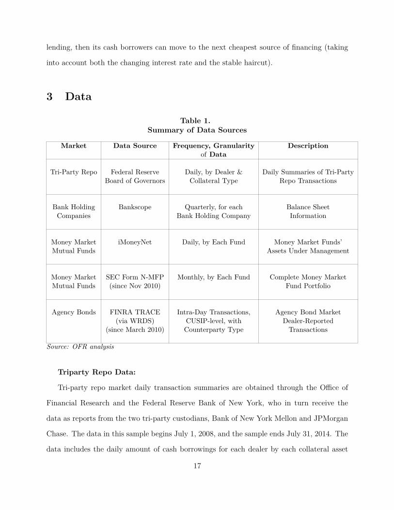
3 Data
Table 1.Summary of Data Sources
Market Data Source Frequency, Granularityof Data
Description
Tri-Party Repo Federal ReserveBoard of Governors
Daily, by Dealer &Collateral Type
Daily Summaries of Tri-PartyRepo Transactions
Bank HoldingCompanies
Bankscope Quarterly, for eachBank Holding Company
Balance SheetInformation
Money MarketMutual Funds
iMoneyNet Daily, by Each Fund Money Market Funds’Assets Under Management
Money MarketMutual Funds
SEC Form N-MFP(since Nov 2010)
Monthly, by Each Fund Complete Money MarketFund Portfolio
Agency Bonds FINRA TRACE(via WRDS)
(since March 2010)
Intra-Day Transactions,CUSIP-level, withCounterparty Type
Agency Bond MarketDealer-ReportedTransactions
Source: OFR analysis
Triparty Repo Data:
Tri-party repo market daily transaction summaries are obtained through the Office of
Financial Research and the Federal Reserve Bank of New York, who in turn receive the
data as reports from the two tri-party custodians, Bank of New York Mellon and JPMorgan
Chase. The data in this sample begins July 1, 2008, and the sample ends July 31, 2014. The
data includes the daily amount of cash borrowings for each dealer by each collateral asset
17
class, as well as the market value including interest due at the end of the repo. The ratio of
those two quantities gives a measure of the dealer’s overall cost of borrowing in that asset
class (haircut plus interest, aggregated across all the dealer’s counterparties).
I omit July 17, 2008, and April 11, 2013 from the sample, because on those two days I am
missing data from one of the custodian banks. I also omit repos in which the Federal Reserve
Bank of New York is a cash borrower from the sample, because of its role as a regulator,
which causes it to behave very differently from other repo participants.11
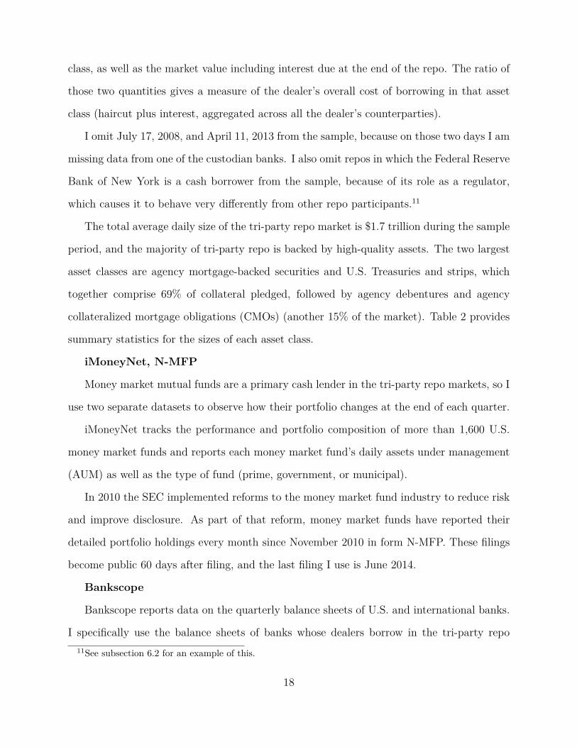
The total average daily size of the tri-party repo market is $1.7 trillion during the sample
period, and the majority of tri-party repo is backed by high-quality assets. The two largest
asset classes are agency mortgage-backed securities and U.S. Treasuries and strips, which
together comprise 69% of collateral pledged, followed by agency debentures and agency
collateralized mortgage obligations (CMOs) (another 15% of the market). Table 2 provides
summary statistics for the sizes of each asset class.
iMoneyNet, N-MFP
Money market mutual funds are a primary cash lender in the tri-party repo markets, so I
use two separate datasets to observe how their portfolio changes at the end of each quarter.
iMoneyNet tracks the performance and portfolio composition of more than 1,600 U.S.
money market funds and reports each money market fund’s daily assets under management
(AUM) as well as the type of fund (prime, government, or municipal).
In 2010 the SEC implemented reforms to the money market fund industry to reduce risk
and improve disclosure. As part of that reform, money market funds have reported their
detailed portfolio holdings every month since November 2010 in form N-MFP. These filings
become public 60 days after filing, and the last filing I use is June 2014.
Bankscope
Bankscope reports data on the quarterly balance sheets of U.S. and international banks.
I specifically use the balance sheets of banks whose dealers borrow in the tri-party repo11See subsection 6.2 for an example of this.
18
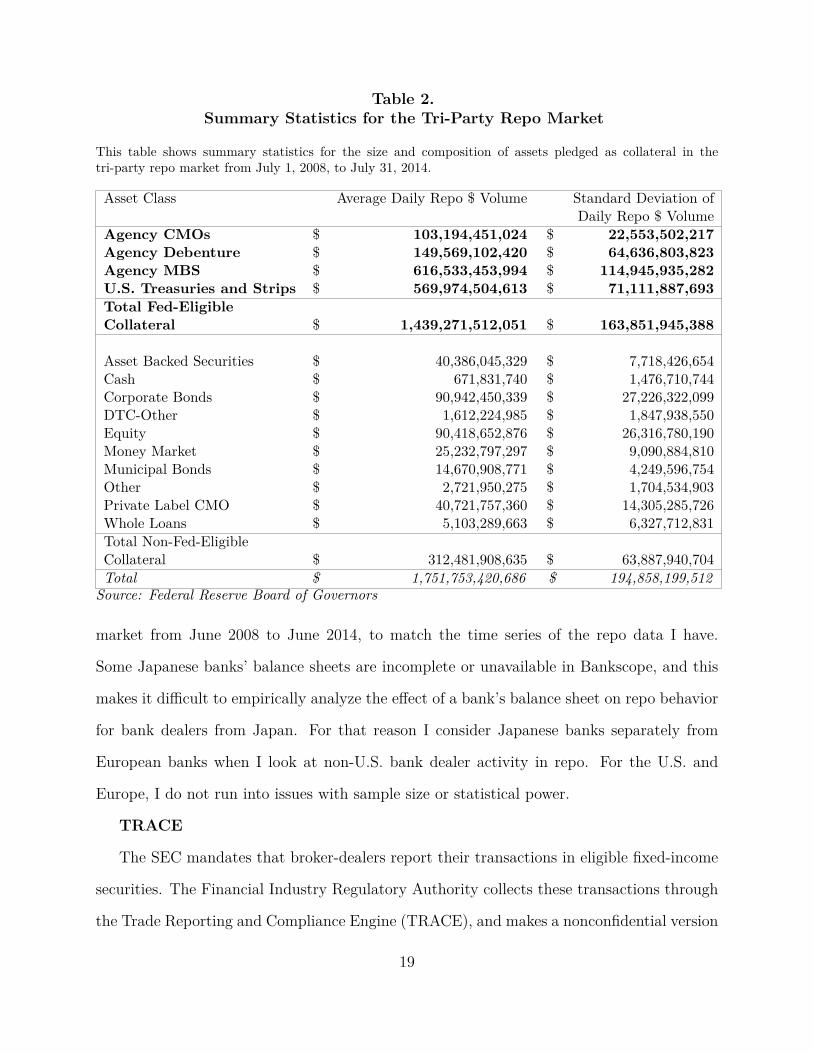
Table 2.Summary Statistics for the Tri-Party Repo Market
This table shows summary statistics for the size and composition of assets pledged as collateral in thetri-party repo market from July 1, 2008, to July 31, 2014.
Asset Class Average Daily Repo $ Volume Standard Deviation ofDaily Repo $ Volume
Agency CMOsAgency DebentureAgency MBSU.S. Treasuries and Strips
$$$$
103,194,451,024149,569,102,420616,533,453,994569,974,504,613
$$$$
22,553,502,21764,636,803,823
114,945,935,28271,111,887,693
Total Fed-EligibleCollateral $ 1,439,271,512,051 $ 163,851,945,388
Asset Backed SecuritiesCashCorporate BondsDTC-OtherEquityMoney MarketMunicipal BondsOtherPrivate Label CMOWhole Loans
$$$$$$$$$$
40,386,045,329671,831,740
90,942,450,3391,612,224,98590,418,652,87625,232,797,29714,670,908,7712,721,950,27540,721,757,3605,103,289,663
$$$$$$$$$$
7,718,426,6541,476,710,744
27,226,322,0991,847,938,55026,316,780,1909,090,884,8104,249,596,7541,704,534,90314,305,285,7266,327,712,831
Total Non-Fed-EligibleCollateral $ 312,481,908,635 $ 63,887,940,704Total $ 1,751,753,420,686 $ 194,858,199,512
Source: Federal Reserve Board of Governors
market from June 2008 to June 2014, to match the time series of the repo data I have.
Some Japanese banks’ balance sheets are incomplete or unavailable in Bankscope, and this
makes it difficult to empirically analyze the effect of a bank’s balance sheet on repo behavior
for bank dealers from Japan. For that reason I consider Japanese banks separately from
European banks when I look at non-U.S. bank dealer activity in repo. For the U.S. and
Europe, I do not run into issues with sample size or statistical power.
TRACE
The SEC mandates that broker-dealers report their transactions in eligible fixed-income
securities. The Financial Industry Regulatory Authority collects these transactions through
the Trade Reporting and Compliance Engine (TRACE), and makes a nonconfidential version
19
of this content available to researchers through Wharton Research Data Services (WRDS),
which I use. Each transaction report identifies the dealer’s counterparty as either another
dealer or a customer, and the report details the security identifier (CUSIP), price, quantity,
and direction of the trade. TRACE reports this data by the type of security, which in WRDS
can be corporate bonds or agency bonds. I use the TRACE agency dataset, which begins in
March 2010 and continues through June 2014.
4 Empirical Results
4.1 Repo Declines Significantly at Quarter-End
The decline in repo is visually apparent and statistically very pronounced. Panel A of Table 3
reports a regression of aggregate repo borrowing in the entire market and by the region of
bank dealers, using indicator variables for each of the five days preceding and following the
end of a quarter. Because the size of the repo market varies over time, I include fixed effects
for each quarter. Column (4) of Table 3 shows that in aggregate, quarter-end repo is $169.4
billion below typical levels. However, on the first day of the quarter, repo strongly rebounds
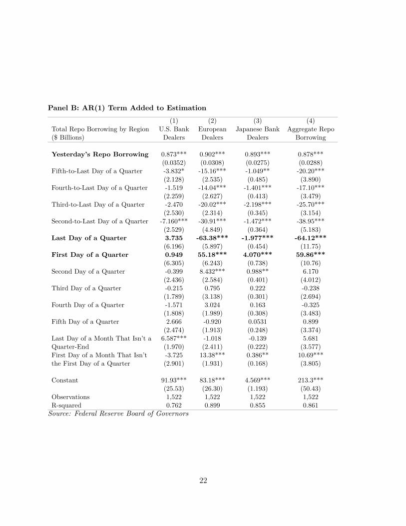
and continues to pick up over the next five days. Panel (B) repeats this analysis, but adds
one-day lagged repo borrowing to account for auto-regression in the data and highlight the
rebound in repo borrowing around the change of a quarter. Columns (2) and (3) of both
Panels (A) and (B) show that this decline and rebound are strongly present in European and
Japanese bank dealers as well. Even though their normal repo borrowing is comparable to
European bank dealers, the U.S. decline in column (1) is an order of magnitude smaller and
largely insignificant. This partially explains why previous studies using U.S. bank holding
company Y-9C statements (such as Owens and Wu (2012) and Downing (2012)) fail to find
seasonality or window dressing in the repo market: of all bank dealers, those of the U.S. do
it the least.
European and Japanese bank dealers reduce their cash borrowing at quarter-end, and20
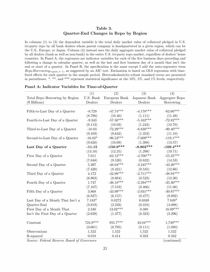
Table 3.Quarter-End Changes in Repo by Region
In columns (1) to (3) the dependent variable is the total daily market value of collateral pledged in U.S.tri-party repo by all bank dealers whose parent company is headquartered in a given region, which can bethe U.S., Europe, or Japan. Column (4) instead uses the daily aggregate market value of collateral pledgedby all dealers (bank as well as non-bank) in the entire U.S. tri-party repo market, regardless of dealers’ homecountries. In Panel A, the regressors are indicator variables for each of the five business days preceding andfollowing a change in calendar quarter, as well as the last and first business day of a month that isn’t theend or start of a quarter. In Panel B, the specification is the same except I add the auto-regressive termRepo Borrowingregion, t−1, as suggested by an AIC test. Estimation is based on OLS regression with time-fixed effects for each quarter in the sample period. Heteroskedasticity-robust standard errors are presentedin parentheses. *, **, and *** represent statistical significance at the 10%, 5%, and 1% levels, respectively.
Panel A: Indicator Variables for Time-of-Quarter
Total Repo Borrowing by Region($ Billions)
(1)U.S. BankDealers
(2)European Bank
Dealers
(3)Japanese Bank
Dealers
(4)Aggregate Repo
Borrowing
Fifth-to-Last Day of a Quarter
Fourth-to-Last Day of a Quarter
Third-to-Last Day of a Quarter
Second-to-Last Day of a Quarter
Last Day of a Quarter
First Day of a Quarter
Second Day of a Quarter
Third Day of a Quarter
Fourth Day of a Quarter
Fifth Day of a Quarter
Last Day of a Month That Isn’t aQuarter-EndFirst Day of a Month ThatIsn’t the First Day of a Quarter
Constant
ObservationsR-squared
-8.729(8.790)-9.343(9.113)-10.83(9.459)-16.82*(9.620)-11.15(13.10)7.011(7.848)5.397(7.420)4.172(6.963)1.747(7.107)3.868(6.827)7.183*(3.819)2.340(2.629)
724.9***(0.661)1,5220.018
-47.74***(10.40)
-57.50***(10.03)
-72.29***(9.642)
-96.53***(10.09)
-150.9***(12.25)
-62.12***(9.520)
-48.04***(8.421)
-42.98***(8.804)
-36.18***(7.519)
-33.99***(6.157)0.0272(2.233)13.02***(1.377)
855.7***(0.795)1,5220.414
-4.178***(1.111)
-5.162***(1.243)
-6.838***(1.353)
-7.609***(1.398)
-8.802***(1.298)
-4.700***(0.832)
-3.245***(0.535)
-2.711***(0.523)
-2.294***(0.466)
-2.031***(0.477)0.0349(0.318)0.388(0.323)
43.04***(0.111)1,5220.323
-62.60***(11.49)
-72.82***(10.70)
-90.40***(11.10)
-119.1***(13.57)
-169.4***(19.71)
-55.35***(14.53)
-43.20***(12.66)
-38.94***(12.30)
-35.30***(11.06)
-30.87***(9.892)7.049*(4.098)16.09***(3.296)
1,749***(1.080)1,5220.342
Source: Federal Reserve Board of Governors (continued)
21
Panel B: AR(1) Term Added to Estimation
Total Repo Borrowing by Region($ Billions)
(1)U.S. BankDealers
(2)EuropeanDealers
(3)Japanese Bank
Dealers
(4)Aggregate Repo
Borrowing
Yesterday’s Repo Borrowing 0.873***(0.0352)
Fifth-to-Last Day of a Quarter -3.832*(2.128)
Fourth-to-Last Day of a Quarter -1.519(2.259)
Third-to-Last Day of a Quarter -2.470(2.530)
Second-to-Last Day of a Quarter -7.160***(2.529)
Last Day of a Quarter 3.735(6.196)
First Day of a Quarter 0.949(6.305)
Second Day of a Quarter -0.399(2.436)
Third Day of a Quarter -0.215(1.789)
Fourth Day of a Quarter -1.571(1.808)
Fifth Day of a Quarter 2.666(2.474)
Last Day of a Month That Isn’t a 6.587***Quarter-End (1.970)First Day of a Month That Isn’t -3.725the First Day of a Quarter (2.901)
Constant 91.93***(25.53)
Observations 1,522R-squared 0.762
0.902***(0.0308)-15.16***(2.535)
-14.04***(2.627)
-20.02***(2.314)
-30.91***(4.849)
-63.38***(5.897)
55.18***(6.243)8.432***(2.584)0.795(3.138)3.024(1.989)-0.920(1.913)-1.018(2.411)13.38***(1.931)
83.18***(26.30)1,5220.899
0.893***(0.0275)-1.049**(0.485)
-1.401***(0.413)
-2.198***(0.345)
-1.472***(0.364)
-1.977***(0.454)
4.070***(0.738)0.988**(0.401)0.222(0.301)0.163(0.308)0.0531(0.248)-0.139(0.222)0.386**(0.168)
4.569***(1.193)1,5220.855
0.878***(0.0288)-20.20***(3.890)
-17.10***(3.479)
-25.70***(3.154)
-38.95***(5.183)
-64.12***(11.75)
59.86***(10.76)6.170(4.012)-0.238(2.694)-0.325(3.483)0.899(3.374)5.681(3.577)10.69***(3.805)
213.3***(50.43)1,5220.861
Source: Federal Reserve Board of Governors
22
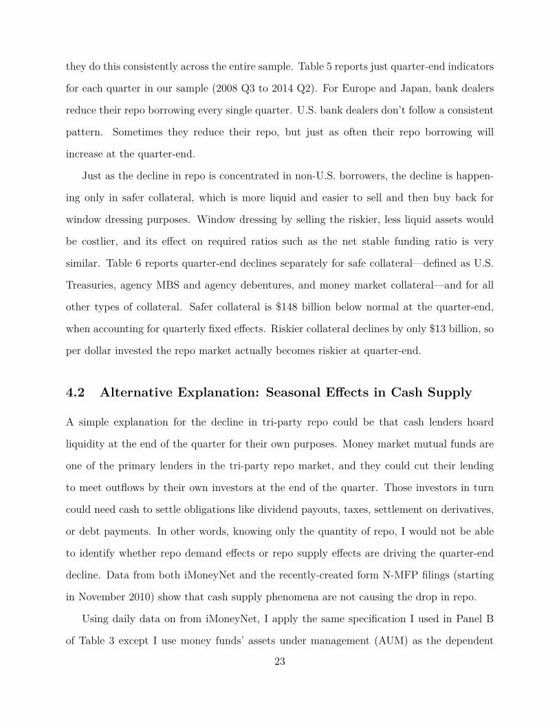
they do this consistently across the entire sample. Table 5 reports just quarter-end indicators
for each quarter in our sample (2008 Q3 to 2014 Q2). For Europe and Japan, bank dealers
reduce their repo borrowing every single quarter. U.S. bank dealers don’t follow a consistent
pattern. Sometimes they reduce their repo, but just as often their repo borrowing will
increase at the quarter-end.
Just as the decline in repo is concentrated in non-U.S. borrowers, the decline is happen-
ing only in safer collateral, which is more liquid and easier to sell and then buy back for
window dressing purposes. Window dressing by selling the riskier, less liquid assets would
be costlier, and its effect on required ratios such as the net stable funding ratio is very
similar. Table 6 reports quarter-end declines separately for safe collateral—defined as U.S.
Treasuries, agency MBS and agency debentures, and money market collateral—and for all
other types of collateral. Safer collateral is $148 billion below normal at the quarter-end,
when accounting for quarterly fixed effects. Riskier collateral declines by only $13 billion, so
per dollar invested the repo market actually becomes riskier at quarter-end.
4.2 Alternative Explanation: Seasonal Effects in Cash Supply
A simple explanation for the decline in tri-party repo could be that cash lenders hoard
liquidity at the end of the quarter for their own purposes. Money market mutual funds are
one of the primary lenders in the tri-party repo market, and they could cut their lending
to meet outflows by their own investors at the end of the quarter. Those investors in turn
could need cash to settle obligations like dividend payouts, taxes, settlement on derivatives,
or debt payments. In other words, knowing only the quantity of repo, I would not be able
to identify whether repo demand effects or repo supply effects are driving the quarter-end
decline. Data from both iMoneyNet and the recently-created form N-MFP filings (starting
in November 2010) show that cash supply phenomena are not causing the drop in repo.
Using daily data on from iMoneyNet, I apply the same specification I used in Panel B
of Table 3 except I use money funds’ assets under management (AUM) as the dependent
23
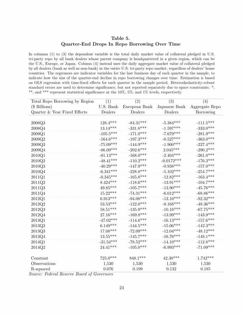
Table 5.Quarter-End Drops In Repo Borrowing Over Time
In columns (1) to (3) the dependent variable is the total daily market value of collateral pledged in U.S.tri-party repo by all bank dealers whose parent company is headquartered in a given region, which can bethe U.S., Europe, or Japan. Column (4) instead uses the daily aggregate market value of collateral pledgedby all dealers (bank as well as non-bank) in the entire U.S. tri-party repo market, regardless of dealers’ homecountries. The regressors are indicator variables for the last business day of each quarter in the sample, toindicate how the size of the quarter-end decline in repo borrowing changes over time. Estimation is basedon OLS regression with time-fixed effects for each quarter in the sample period. Heteroskedasticity-robuststandard errors are used to determine significance, but not reported separately due to space constraints. *,**, and *** represent statistical significance at the 10%, 5%, and 1% levels, respectively.
Total Repo Borrowing by Region($ Billions)Quarter & Year Fixed Effects
(1)U.S. BankDealers
(2)European Bank
Dealers
(3)Japanese Bank
Dealers
(4)Aggregate Repo
Borrowing
2008Q3 128.4***2008Q4 13.14***2009Q1 -105.5***2009Q2 -164.6***2009Q3 -75.09***2009Q4 -86.09***2010Q1 -81.13***2010Q2 -48.41***2010Q3 -40.29***2010Q4 -6.341***2011Q1 -0.345***2011Q2 8.424***2011Q3 49.85***2011Q4 15.22***2012Q1 6.913***2012Q2 53.53***2012Q3 58.51***2012Q4 27.16***2013Q1 -47.02***2013Q2 6.149***2013Q3 17.08***2013Q4 13.55***2014Q1 -31.54***2014Q2 24.41***
Constant 725.0***Observations 1,530R-squared 0.076
-84.31***-331.8***-171.0***-197.3***-144.9***-202.6***-168.0***-110.2***-147.9***-228.8***-165.8***-118.6***-105.7***-74.31***-94.08***-122.0***-135.9***-169.8***-114.6***-144.5***-72.09***-145.7***-78.52***-105.0***
848.1***1,5300.199
-5.384***-1.597***-7.679***-0.527***-1.900***2.045***-2.404***-0.0172***-0.938***-5.102***-12.82***-13.91***-13.90***-6.012***-13.10***-8.168***-10.16***-13.99***-16.13***-15.06***-12.04***-16.76***-14.10***-6.993***
42.38***1,5300.132
-111.5***-333.0***-281.9***-363.0***-227.4***-290.2***-261.0***-176.3***-157.0***-254.7***-163.4***-104.7***-45.76***-68.86***-92.32***-48.36***-67.75***-143.9***-157.6***-142.3***-48.12***-148.1***-112.8***-71.09***
1,742***1,5300.185
Source: Federal Reserve Board of Governors
24
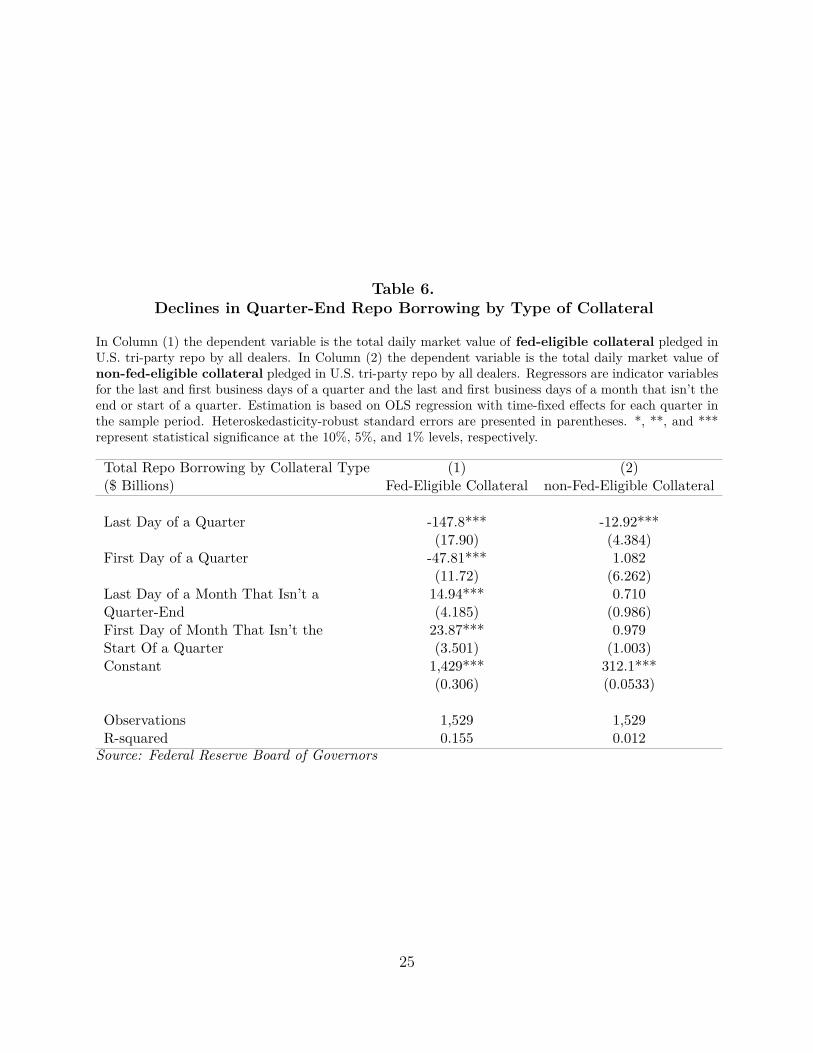
Table 6.Declines in Quarter-End Repo Borrowing by Type of Collateral
In Column (1) the dependent variable is the total daily market value of fed-eligible collateral pledged inU.S. tri-party repo by all dealers. In Column (2) the dependent variable is the total daily market value ofnon-fed-eligible collateral pledged in U.S. tri-party repo by all dealers. Regressors are indicator variablesfor the last and first business days of a quarter and the last and first business days of a month that isn’t theend or start of a quarter. Estimation is based on OLS regression with time-fixed effects for each quarter inthe sample period. Heteroskedasticity-robust standard errors are presented in parentheses. *, **, and ***represent statistical significance at the 10%, 5%, and 1% levels, respectively.
Total Repo Borrowing by Collateral Type($ Billions)
(1)Fed-Eligible Collateral
(2)non-Fed-Eligible Collateral
Last Day of a Quarter
First Day of a Quarter
Last Day of a Month That Isn’t aQuarter-EndFirst Day of Month That Isn’t theStart Of a QuarterConstant
ObservationsR-squared
-147.8***(17.90)
-47.81***(11.72)14.94***(4.185)23.87***(3.501)1,429***(0.306)
1,5290.155
-12.92***(4.384)1.082(6.262)0.710(0.986)0.979(1.003)312.1***(0.0533)
1,5290.012
Source: Federal Reserve Board of Governors
25
variable, rather than total tri-party repo market borrowing. Table 7 shows that money funds
do see outflows at the end of the quarter followed by inflows at the start of the new quarter,
but they are less than a tenth the size of repo declines. Additionally, there is no significant
decline in MMFs’ AUM before the last day of the quarter, unlike the accelerating drawdown
over several days that happens in repo. Therefore, money fund outflows cannot explain the
size and scope of the repo market effect.
Although money funds are one of the two primary types of cash lenders in tri-party
repo, they are not the only tri-party cash provider. Securities lending agents also reinvest
cash collateral in tri-party repo, so a regular and sudden quarter-end unwinding of securities
lending could also pull cash out of the tri-party repo system. Although I do not have data
on securities lending covering this period, I do have data on money market funds’ detailed
portfolio holdings from the new form N-MFP, which contradicts this account.
Since form N-MFP is a monthly, not quarterly, filing, I do not have to worry about
money funds themselves window-dressing their quarter-end holdings any more than they
would for a different month. Therefore, I can compare quarter-end holdings to holdings at
the end of other months to see what changes. Table 8 shows that at the quarter-end, money
funds’ repo holdings decline, even though their AUM does not decline significantly. I do
not report non-repo asset classes in the table because no other reported investment classes
have significant quarter-end changes. However, I do report money market funds’ uninvested
cash, which is the remainder from subtracting the sum of all its investments from a fund’s
reported AUM.12
Table 9 reports that money funds are holding excess cash at the end of the quarter,
both individually and in aggregate. Money market funds specialize in making short-term
investments, but prime and government/agency MMFs together cannot find temporary in-
vestments for nearly $20 billion dollars,13 meaning there is an excess—not a shortage—of12Normally, a money fund will actually have a cash balance of zero or just slightly less than zero, with any
shortfall due to the fact that a sponsor may have invested its own money in the fund to support it, which isnot reflected in the fund’s AUM.
13$12.62 billion for prime MMFs, $7.188 billion for govt/agency MMFs, see column (4) of Table 9.
26
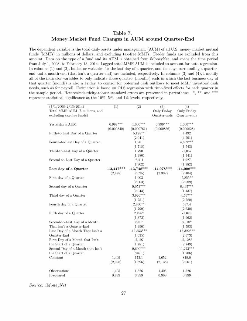
Table 7.Money Market Fund Changes in AUM around Quarter-End
The dependent variable is the total daily assets under management (AUM) of all U.S. money market mutualfunds (MMFs) in millions of dollars, and excluding tax-free MMFs. Feeder funds are excluded from thisamount. Data on the type of a fund and its AUM is obtained from iMoneyNet, and spans the time periodfrom July 1, 2008, to February 13, 2014. Lagged total MMF AUM is included to account for auto-regression.In columns (1) and (2), indicator variables for the last day of a quarter, and the days surrounding a quarter-end and a month-end (that isn’t a quarter-end) are included, respectively. In columns (3) and (4), I modifyall of the indicator variables to only indicate those quarter- (month-) ends in which the last business day ofthat quarter (month) is also a Friday, to control for potential cash outflows to meet MMF investors’ cashneeds, such as for payroll. Estimation is based on OLS regression with time-fixed effects for each quarter inthe sample period. Heteroskedasticity-robust standard errors are presented in parentheses. *, **, and ***represent statistical significance at the 10%, 5%, and 1% levels, respectively.
(7/1/2008–2/13/2014) (1) (2) (3) (4)Total MMF AUM ($ millions, and Only Friday Only Fridayexcluding tax-free funds) Quarter-ends Quarter-ends
Yesterday’s AUM 0.999*** 1.000*** 0.999*** 1.000***(0.000840) (0.000761) (0.000856) (0.000828)
Fifth-to-Last Day of a Quarter 5,125** 4,492(2,041) (4,501)
Fourth-to-Last Day of a Quarter 1,981 4,689***(1,718) (1,543)
Third-to-Last Day of a Quarter 1,790 -1,067(1,380) (1,441)
Second-to-Last Day of a Quarter -2,411 1,927(1,902) (1,982)
Last day of a Quarter -12,447*** -13,748*** -14,078*** -14,008***(2,425) (2,625) (2,392) (2,404)
First day of a Quarter 1,003 -5,855**(2,603) (2,689)
Second day of a Quarter 9,053*** 6,495***(2,043) (1,437)
Third day of a Quarter 3,926*** 4,567**(1,251) (2,280)
Fourth day of a Quarter 2,930** 537.4(1,299) (2,630)
Fifth day of a Quarter 2,495* -1,078(1,372) (1,962)
Second-to-Last Day of a Month 298.7 3,018*That Isn’t a Quarter-End (1,390) (1,593)Last Day of a Month That Isn’t a -12,553*** -13,322***Quarter-End (1,635) (2,673)First Day of a Month that Isn’t -2,197 -5,128*the Start of a Quarter (1,781) (2,749)Second Day of a Month that Isn’t 9,600*** 11,223***the Start of a Quarter (846.1) (1,206)Constant 1,409 172.1 1,652 819.0
(2,098) (1,896) (2,138) (2,061)
Observations 1,405 1,526 1,405 1,526R-squared 0.999 0.999 0.999 0.999
Source: iMoneyNet
27
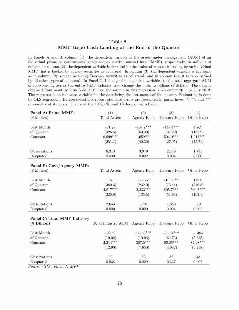
Table 8.MMF Repo Cash Lending at the End of the Quarter
In Panels A and B, column (1), the dependent variable is the assets under management (AUM) of anindividual prime or government/agency money market mutual fund (MMF), respectively, in millions ofdollars. In column (2), the dependent variable is the total market value of repo cash lending by an individualMMF that is backed by agency securities as collateral. In column (3), the dependent variable is the sameas in column (2), except receiving Treasury securities as collateral, and in column (4), it is repo backedby all other types of collateral. In Panel C, I change the dependent variables to the total aggregate AUMor repo lending across the entire MMF industry, and change the units to billions of dollars. The data isobtained from monthly form N-MFP filings, the sample in this regression is November 2011 to July 2013.The regressor is an indicator variable for the date being the last month of the quarter. Estimation is doneby OLS regression. Heteroskedasticity-robust standard errors are presented in parentheses. *, **, and ***represent statistical significance at the 10%, 5%, and 1% levels, respectively.
Panel A: Prime MMFs (1) (2) (3) (4)($ Million) Total Assets Agency Repo Treasury Repo Other Repo
Last Month -21.72 -192.7*** -142.4*** 4.769of Quarter (426.5) (63.09) (37.29) (131.9)Constant 6,999*** 1,052*** 504.0*** 1,211***
(251.1) (40.30) (27.95) (75.71)
Observations 6,313 3,979 2,779 1,791R-squared 0.000 0.002 0.004 0.000
Panel B: Govt/Agency MMFs($ Million) Total Assets Agency Repo Treasury Repo Other Repo
Last Month 115.1 -22.77 -185.0** 112.8of Quarter (380.6) (232.0) (73.44) (316.3)Constant 4,817*** 2,233*** 805.7*** 560.3***
(220.0) (135.5) (51.63) (193.1)
Observations 2,653 1,704 1,389 119R-squared 0.000 0.000 0.004 0.001
Panel C: Total MMF Industry($ Billion) Total Industry AUM Agency Repo Treasury Repo Other Repo
Last Month -22.80 -35.83*** -25.64*** -1.384of Quarter (19.92) (10.96) (6.173) (5.685)Constant 2,214*** 307.5*** 96.06*** 84.28***
(12.90) (7.650) (4.087) (3.258)
Observations 32 32 32 32R-squared 0.038 0.229 0.337 0.002Source: SEC Form N-MFP
28
cash supply at quarter-end. If securities lenders or other unobserved tri-party repo cash sup-
pliers were choosing to cut their repo lending and dealers’ demand for repo was unchanged,
dealers would have been able substitute and borrow cash from money market funds instead,
and money market funds would not have this excess cash.
4.3 Dealer Leverage Explains Non-U.S. Bank Dealer Repo Quarter-
End Declines
Earlier tests in this paper showed no evidence to support a cash supply-driven effect, but
here I do find evidence consistent with a cash demand-driven effect. Among the differences
across capital regulation regimes in the U.S., Europe, and Japan, the most relevant aspect for
this study is the reporting requirement. U.S. banks are required to report capital ratios for
the last day of the quarter as well as an average across all days of the quarter. In contrast,
non-U.S. banks can simply report for the last day of the quarter. Therefore, U.S. banks
have very little incentive to window-dress their balance sheet at the end of the quarter—it
will not affect their capital requirements any more than a deviation any other time in the
quarter would. If this is indeed what’s driving the difference I observe between U.S. and
non-U.S. bank dealers, I would expect more levered non-U.S. bank dealers to be more likely
to window-dress.
I link the tri-party repo holdings for each bank dealer to that bank’s quarterly balance
sheet, using data obtained from BankScope. One limitation of BankScope is that it does not
contain data on all banks, especially Japanese banks. However, for the U.S. and Europe, I
am able to link almost all dealers to their banks. In Table 10, I test a fixed-effects regression
model for each region, where I supplement my end-of-quarter indicator variables with the
linked bank balance sheet for the previous quarter. To specifically test whether highly levered
banks are reducing their dealers’ repo borrowing at the end of the quarter to report lower
leverage, I interact the bank’s Tier 1 capital ratio from the previous quarter with an indicator
for the last day of the current quarter. A higher Tier 1 capital ratio means less leverage, so29
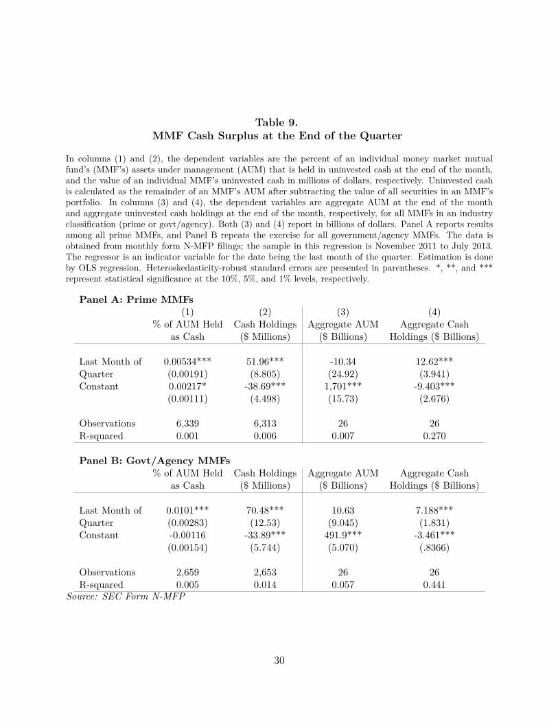
Table 9.MMF Cash Surplus at the End of the Quarter
In columns (1) and (2), the dependent variables are the percent of an individual money market mutualfund’s (MMF’s) assets under management (AUM) that is held in uninvested cash at the end of the month,and the value of an individual MMF’s uninvested cash in millions of dollars, respectively. Uninvested cashis calculated as the remainder of an MMF’s AUM after subtracting the value of all securities in an MMF’sportfolio. In columns (3) and (4), the dependent variables are aggregate AUM at the end of the monthand aggregate uninvested cash holdings at the end of the month, respectively, for all MMFs in an industryclassification (prime or govt/agency). Both (3) and (4) report in billions of dollars. Panel A reports resultsamong all prime MMFs, and Panel B repeats the exercise for all government/agency MMFs. The data isobtained from monthly form N-MFP filings; the sample in this regression is November 2011 to July 2013.The regressor is an indicator variable for the date being the last month of the quarter. Estimation is doneby OLS regression. Heteroskedasticity-robust standard errors are presented in parentheses. *, **, and ***represent statistical significance at the 10%, 5%, and 1% levels, respectively.
Panel A: Prime MMFs(1)
% of AUM Heldas Cash
(2)Cash Holdings($ Millions)
(3)Aggregate AUM
($ Billions)
(4)Aggregate Cash
Holdings ($ Billions)
Last Month of 0.00534*** 51.96*** -10.34 12.62***Quarter (0.00191) (8.805) (24.92) (3.941)Constant 0.00217* -38.69*** 1,701*** -9.403***
(0.00111) (4.498) (15.73) (2.676)
Observations 6,339 6,313 26 26R-squared 0.001 0.006 0.007 0.270
Panel B: Govt/Agency MMFs% of AUM Held
as CashCash Holdings($ Millions)
Aggregate AUM($ Billions)
Aggregate CashHoldings ($ Billions)
Last Month of 0.0101*** 70.48*** 10.63 7.188***Quarter (0.00283) (12.53) (9.045) (1.831)Constant -0.00116 -33.89*** 491.9*** -3.461***
(0.00154) (5.744) (5.070) (.8366)
Observations 2,659 2,653 26 26R-squared 0.005 0.014 0.057 0.441
Source: SEC Form N-MFP
30
if window dressing is driving repo declines, this regression coefficient must be positive. The
first row of column (3) shows that for European bank dealers, this coefficient is positive and
significant, suggesting window dressing incentives do explain their repo borrowing. Moreover,
the same coefficient for U.S. bank dealers in column (2) is insignificant and actually negative,
just as we would expect given their quarter-average reporting requirement. Therefore, this
cross-region test seems to confirm that the difference between U.S. and European bank dealer
behavior is explained by window dressing.
4.4 Joint Model Test
Thus far, in looking at cash suppliers and cash demanders separately, evidence rejects a
supply shift and favors a demand shift. However, to confirm this result, I use a proxy for
the price of repo borrowing (the sum of the haircut and the repo rate) in each asset class.
With this dealer-specific measure of the price of repo, I can test both quantity and price at
the end of the quarter, to determine whether the dominant effect is from cash demand or
supply.
Because the cost of borrowing in repo is dealer-specific as well as asset class-specific, I
test quarter-end effects in quantity and price of repo by each dealer, in each of their collateral
types. I control for variation between dealers and between asset types by adding fixed effects
for each quarter, dealer, and asset class in Table 11. Column (4) shows that while non-U.S.
bank dealers do less repo at the end of the quarter, the cost to borrow does not rise at all—in
fact, the coefficient is slightly negative.14
4.5 Identification Using the Dealer-Lender Network
One limitation of my analysis so far is that it still suffers from the potential for omitted
variable bias. Non-U.S. bank dealers may be borrowing from a different set of lenders than14In contrast, U.S. bank dealers do not window-dress, and their borrowing cost even rises slightly (and
there is no reversal at the start of the new quarter).
31
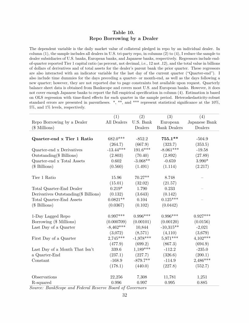
Table 10.Repo Borrowing by a Dealer
The dependent variable is the daily market value of collateral pledged in repo by an individual dealer. Incolumn (1), the sample includes all dealers in U.S. tri-party repo, in columns (2) to (4), I reduce the sample todealer subsidiaries of U.S. banks, European banks, and Japanese banks, respectively. Regressors include end-of-quarter reported Tier 1 capital ratio (as percent, not decimal, i.e., 12 not .12), and the total value in billionsof dollars of derivatives and of total assets for the dealer’s parent bank the prior quarter. These regressorsare also interacted with an indicator variable for the last day of the current quarter (“Quarter-end”). Ialso include time dummies for the days preceding a quarter- or month-end, as well as the days following anew quarter; however, they are not reported due to page constraints but available upon request. Quarterlybalance sheet data is obtained from Bankscope and covers most U.S. and European banks. However, it doesnot cover enough Japanese banks to report the full empirical specification in column (4). Estimation is basedon OLS regression with time-fixed effects for each quarter in the sample period. Heteroskedasticity-robuststandard errors are presented in parentheses. *, **, and *** represent statistical significance at the 10%,5%, and 1% levels, respectively.
Repo Borrowing by a Dealer($ Millions)
(1)All Dealers
(2)U.S. BankDealers
(3)European
Bank Dealers
(4)Japanese Bank
Dealers
Quarter-end x Tier 1 Ratio 682.0*** -852.2(264.7) (667.9)
Quarter-end x Derivatives -13.44*** 191.6***Outstanding($ Billions) (2.803) (70.40)Quarter-end x Total Assets 0.602 -3.068**($ Billions) (0.560) (1.491)
Tier 1 Ratio 15.96 70.27**(15.01) (32.02)
Total Quarter-End Dealer 0.219* 1.790Derivatives Outstanding($ Billions) (0.132) (3.643)Total Quarter-End Assets 0.0821** 0.104($ Billions) (0.0367) (0.102)
1-Day Lagged Repo 0.997*** 0.996***Borrowing ($ Millions) (0.000709) (0.00101)Last Day of a Quarter -8,462*** 10,844
(3,072) (8,571)First Day of a Quarter 2,745*** -1,978***
(477.9) (699.2)Last Day of a Month That Isn’t 339.6 1,189***a Quarter-End (237.1) (227.7)Constant -168.9 -879.7**
(178.1) (440.0)
Observations 22,256 7,308R-squared 0.996 0.997
755.1**(323.7)
-8.061***(2.892)-0.659(1.114)
8.748(21.57)0.233(0.142)0.125***(0.0442)
0.996***(0.00120)-10,315**(4,110)5,971***(867.3)-112.2(326.6)-114.9(227.8)
11,7810.995
-504.9(353.5)-19.58(27.89)3.990*(2.217)
–
–
–
0.927***(0.0156)-2,021(3,679)4,102***(694.9)-235.0(200.1)2,486***(552.7)
1,2510.885
Source: BankScope and Federal Reserve Board of Governors32
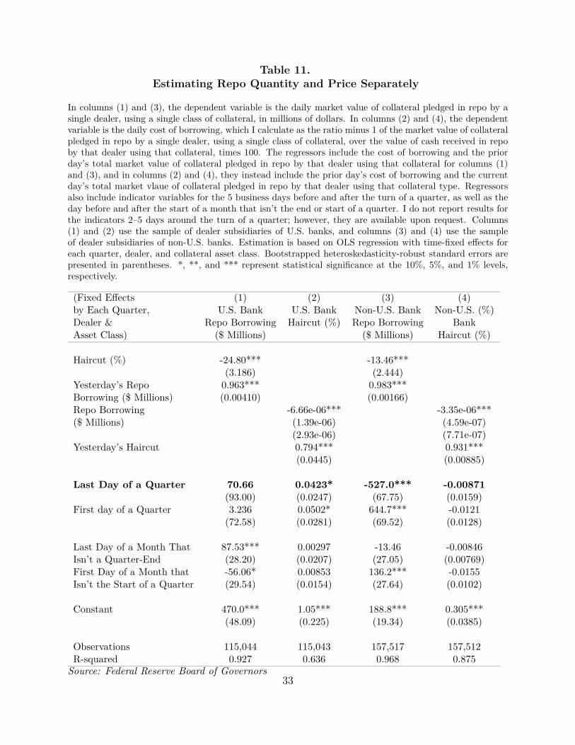
Table 11.Estimating Repo Quantity and Price Separately
In columns (1) and (3), the dependent variable is the daily market value of collateral pledged in repo by asingle dealer, using a single class of collateral, in millions of dollars. In columns (2) and (4), the dependentvariable is the daily cost of borrowing, which I calculate as the ratio minus 1 of the market value of collateralpledged in repo by a single dealer, using a single class of collateral, over the value of cash received in repoby that dealer using that collateral, times 100. The regressors include the cost of borrowing and the priorday’s total market value of collateral pledged in repo by that dealer using that collateral for columns (1)and (3), and in columns (2) and (4), they instead include the prior day’s cost of borrowing and the currentday’s total market vlaue of collateral pledged in repo by that dealer using that collateral type. Regressorsalso include indicator variables for the 5 business days before and after the turn of a quarter, as well as theday before and after the start of a month that isn’t the end or start of a quarter. I do not report results forthe indicators 2–5 days around the turn of a quarter; however, they are available upon request. Columns(1) and (2) use the sample of dealer subsidiaries of U.S. banks, and columns (3) and (4) use the sampleof dealer subsidiaries of non-U.S. banks. Estimation is based on OLS regression with time-fixed effects foreach quarter, dealer, and collateral asset class. Bootstrapped heteroskedasticity-robust standard errors arepresented in parentheses. *, **, and *** represent statistical significance at the 10%, 5%, and 1% levels,respectively.
(Fixed Effectsby Each Quarter,Dealer &Asset Class)
(1)U.S. Bank
Repo Borrowing($ Millions)
(2)U.S. BankHaircut (%)
(3)Non-U.S. BankRepo Borrowing
($ Millions)
(4)Non-U.S. (%)
BankHaircut (%)
Haircut (%) -24.80***(3.186)
Yesterday’s Repo 0.963***Borrowing ($ Millions) (0.00410)Repo Borrowing($ Millions)
Yesterday’s Haircut
Last Day of a Quarter 70.66(93.00)
First day of a Quarter 3.236(72.58)
Last Day of a Month That 87.53***Isn’t a Quarter-End (28.20)First Day of a Month that -56.06*Isn’t the Start of a Quarter (29.54)
Constant 470.0***(48.09)
Observations 115,044R-squared 0.927
-6.66e-06***(1.39e-06)(2.93e-06)0.794***(0.0445)
0.0423*(0.0247)0.0502*(0.0281)
0.00297(0.0207)0.00853(0.0154)
1.05***(0.225)
115,0430.636
-13.46***(2.444)0.983***(0.00166)
-527.0***(67.75)644.7***(69.52)
-13.46(27.05)136.2***(27.64)
188.8***(19.34)
157,5170.968
-3.35e-06***(4.59e-07)(7.71e-07)0.931***(0.00885)
-0.00871(0.0159)-0.0121(0.0128)
-0.00846(0.00769)-0.0155(0.0102)
0.305***(0.0385)
157,5120.875
Source: Federal Reserve Board of Governors33
U.S. bank dealers, and those lenders may face different shocks at the end of the quarter.
To control for any other potential cash lender effects, I use an additional data set on the
network of tri-party repo lending since 2011. Similar to Khwaja and Mian (2008), I can use
the network to examine the quarter-end effect within a cash lender using both lender and
time-fixed effects. Table 12 reports that within a single lender, quarter-end repo borrowing
by European bank dealers drops 13.6%, while U.S. and Japanese bank dealer borrowing is
not significantly affected.
In a further test, I use a subset of the dealer-investor network that allows me to identify
price effects in the haircut and the repo rate separately. Since November 2010, money market
funds have published complete end-of-month portfolio holdings, including all repurchase
transactions and the haircut and rate applied on the underlying collateral15. To fully identify
price and quantity effects, I collect and use this data on the sub-network of tri-party repo
transactions where money market funds are the cash investor. Table 13 shows that while
money funds lend less to European dealers at quarter-end, repo rates drop at quarter-end
for both U.S. and European bank borrowers and haircuts are not significantly affected for
any participants. This drop in both quantity (for European banks) and in market price (via
the repo rate) is consistent with a shock to cash demand rather than cash supply, which
supports window dressing as the likely explanation for the quarter-end repo anomaly.
5 Robustness Tests
5.1 Unit Root
If repo borrowing follows a unit root process, this might lead to a problem of spurious
regression. I test for unit roots in the quantity of repo borrowing using an Augmented Dickey-
Fuller test allowing for drift in the series and find rejection of that hypothesis. Because I am15A recent paper by Hu, Pan, and Wang (2014) uses this N-MFP filing data to conduct an extensive survey
of tri-party repo pricing practices, and is the only other paper I am aware of which takes advantage of thispricing data.
34
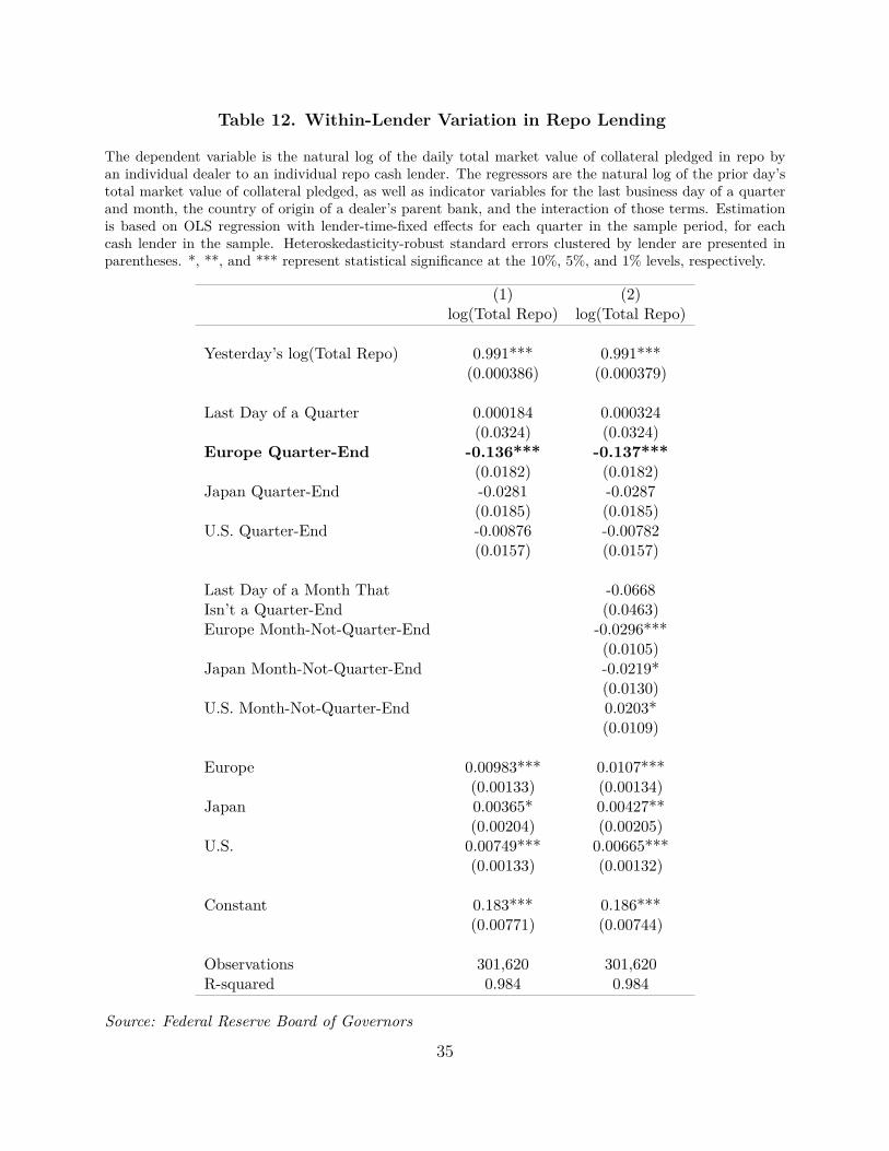
Table 12. Within-Lender Variation in Repo Lending
The dependent variable is the natural log of the daily total market value of collateral pledged in repo byan individual dealer to an individual repo cash lender. The regressors are the natural log of the prior day’stotal market value of collateral pledged, as well as indicator variables for the last business day of a quarterand month, the country of origin of a dealer’s parent bank, and the interaction of those terms. Estimationis based on OLS regression with lender-time-fixed effects for each quarter in the sample period, for eachcash lender in the sample. Heteroskedasticity-robust standard errors clustered by lender are presented inparentheses. *, **, and *** represent statistical significance at the 10%, 5%, and 1% levels, respectively.
(1) (2)log(Total Repo) log(Total Repo)
Yesterday’s log(Total Repo) 0.991*** 0.991***(0.000386) (0.000379)
Last Day of a Quarter 0.000184 0.000324(0.0324) (0.0324)
Europe Quarter-End -0.136*** -0.137***(0.0182) (0.0182)
Japan Quarter-End -0.0281 -0.0287(0.0185) (0.0185)
U.S. Quarter-End -0.00876 -0.00782(0.0157) (0.0157)
Last Day of a Month That -0.0668Isn’t a Quarter-End (0.0463)Europe Month-Not-Quarter-End -0.0296***
(0.0105)Japan Month-Not-Quarter-End -0.0219*
(0.0130)U.S. Month-Not-Quarter-End 0.0203*
(0.0109)
Europe 0.00983*** 0.0107***(0.00133) (0.00134)
Japan 0.00365* 0.00427**(0.00204) (0.00205)
U.S. 0.00749*** 0.00665***(0.00133) (0.00132)
Constant 0.183*** 0.186***(0.00771) (0.00744)
Observations 301,620 301,620R-squared 0.984 0.984
Source: Federal Reserve Board of Governors
35
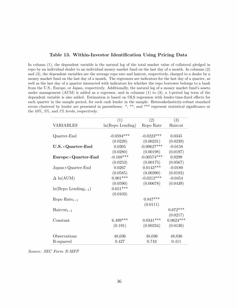
Table 13. Within-Investor Identification Using Pricing Data
In column (1), the dependent variable is the natural log of the total market value of collateral pledged inrepo by an individual dealer to an individual money market fund on the last day of a month. In columns (2)and (3), the dependent variables are the average repo rate and haircut, respectively, charged to a dealer by amoney market fund on the last day of a month. The regressors are indicators for the last day of a quarter, aswell as the last day of a quarter interacted with indicators for whether the repo borrower belongs to a bankfrom the U.S., Europe, or Japan, respectively. Additionally, the natural log of a money market fund’s assetsunder management (AUM) is added as a regressor, and in columns (1) to (3), a 1-period lag term of thedependent variable is also added. Estimation is based on OLS regression with lender-time-fixed effects foreach quarter in the sample period, for each cash lender in the sample. Heteroskedasticity-robust standarderrors clustered by lender are presented in parentheses. *, **, and *** represent statistical significance atthe 10%, 5%, and 1% levels, respectively.
(1) (2) (3)VARIABLES ln(Repo Lending) Repo Rate Haircut
Quarter-End -0.0594*** -0.0223*** 0.0345(0.0228) (0.00231) (0.0239)
U.S.×Quarter-End 0.0305 -0.00627*** -0.0158(0.0280) (0.00198) (0.0197)
Europe×Quarter-End -0.168*** -0.00574*** 0.0299(0.0253) (0.00175) (0.0567)
Japan×Quarter-End 0.0267 0.0143*** -0.0180(0.0585) (0.00390) (0.0183)
∆ ln(AUM) 0.901*** -0.0212*** -0.0454(0.0590) (0.00678) (0.0439)
ln(Repo Lendingt−1) 0.651***(0.0103)
Repo Ratet−1 0.847***(0.0111)
Haircutt−1 0.672***(0.0217)
Constant 6.499*** 0.0341*** 0.0624***(0.191) (0.00234) (0.0130)
Observations 48,036 48,036 48,036R-squared 0.427 0.743 0.411
Source: SEC Form N-MFP
36
also testing repo borrowing at the dealer level, I further test for unit roots across the panel
using a Fisher-type Augmented Dickey-Fuller test, and again reject the null hypothesis that
repo borrowing is a unit root process.
If repo borrowing is not a unit root process but is actually near unit root, my tests for a
unit root would suffer from reduced power. Therefore, I also test for window dressing using
changes in logs rather than an AR(1) specification. Again, I find a significant quarter-end
drop and subsequent rebound in repo borrowing for non-U.S. banks, which is concentrated
in highly levered banks and in repo backed by safe, liquid collateral.
5.2 Panel VAR
I chose to use simultaneous equations for my main empirical strategy because quarter-ends
obviously arrive exogenously. However, to test the identification of my model of supply and
demand, I used a vector auto-regression (VAR) approach. Because tri-party repo haircuts
are dealer– and collateral-specific, I run a panel VAR at the dealer and asset-class level.
Standard model selection technique (AIC) suggests I use 1-period lags. My panel VAR
results are still consistent with window dressing: dealer leverage predicts significantly lower
quarter-end repo borrowing, although I do not retain significance on other balance sheet
measures.
5.3 U.S. Bank Holding Company Data
Other researchers have used data on U.S. bank holding companies (BHCs) to find evidence of
window dressing by U.S. banks. This is inconsistent with my results using the tri-party repo
data, in which I find that window dressing was concentrated in highly leveraged non-U.S.
BHCs. The most compelling results are from Owens and Wu (2012), who use public reports
filed by BHCs in form Y-9C. These reports include the quarter-average and quarter-end
balance sheet data of these banks, and those authors take the discrepancy between those
two measures as evidence of window dressing. To test their result, I repeat their analysis37
using Y-9C data from 2001 through 2013, which I obtain through WRDS. Column (1) of
Table 14 reports similar findings to their Table (4) Column (1): window dressing is indeed
concentrated among BHCs with high leverage.
In Columns (2) and (3), I divide the sample into BHCs that are U.S.-based, and those
bank holding companies that are subsidiaries of a non-U.S. parent.16 The effect of leverage is
entirely concentrated in the few non-U.S. BHCs, and the size effect is quite nearly captured by
non-U.S. BHCs as well. Additions to loan loss reserves during the prior quarter are intended
to account for non-window dressing pressures to de-leverage, and this effect remains for the
U.S. BHCs but not the non-U.S. BHCs. These results are consistent with my findings in
tri-party repo: non-U.S. bank holding companies window-dress and thereby improve the
appearance of their parents’ own financial statements.
6 Spillover Effects from Window Dressing
6.1 Agency Bond Markets
Repurchase agreements give cash in exchange for collateral, and when a dealer decides not
to repo an asset, they must either find alternative financing or sell the asset. Repo window
dressing is concentrated in safe assets: Treasuries, agency MBS and agency bonds, and
money market assets (e.g., CDs). Since March 2010, the Financial Industry Regulatory
Authority (FINRA) has collected data on all agency bond transactions involving dealers,
and made them available to researchers through WRDS.17 In this subsection, I use this
data, including the price, quantity, time of execution and settlement, and direction (dealer-
to-dealer or dealer buying/selling to a non-dealer) of each trade, to examine the impact of
dealer window dressing on market quality for agency bonds.16I also impose the same requirement as Owens and Wu (2012) that these bank holding companies have
total consolidated assets greater than $500 million.17I am unable to locate high-frequency data on Treasury transactions, and in a follow-up extension to
this paper, I am currently processing data from FINRA’s new TRACE dataset of agency MBS transactions,which are not included in this paper.
38
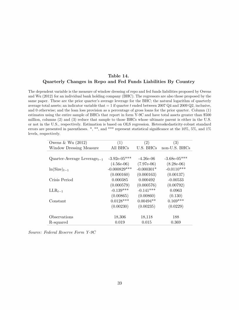
Table 14.Quarterly Changes in Repo and Fed Funds Liabilities By Country
The dependent variable is the measure of window dressing of repo and fed funds liabilities proposed by Owensand Wu (2012) for an individual bank holding company (BHC). The regressors are also those proposed by thesame paper. These are the prior quarter’s average leverage for the BHC; the natural logarithm of quarterlyaverage total assets; an indicator variable that = 1 if quarter t ended between 2007 Q4 and 2009 Q2, inclusive,and 0 otherwise; and the loan loss provision as a percentage of gross loans for the prior quarter. Column (1)estimates using the entire sample of BHCs that report in form Y-9C and have total assets greater than $500million, columns (2) and (3) reduce that sample to those BHCs whose ultimate parent is either in the U.S.or not in the U.S., respectively. Estimation is based on OLS regression. Heteroskedasticity-robust standarderrors are presented in parentheses. *, **, and *** represent statistical significance at the 10%, 5%, and 1%levels, respectively.
Owens & Wu (2012) (1) (2) (3)Window Dressing Measure All BHCs U.S. BHCs non-U.S. BHCs
Quarter-Average Leveraget−1 -3.92e-05*** -4.26e-06 -3.68e-05***(4.56e-06) (7.97e-06) (8.28e-06)
ln(Size)t−1 -0.000829*** -0.000301* -0.0110***(0.000160) (0.000163) (0.00137)
Crisis Period 0.000385 0.000492 -0.00533(0.000579) (0.000576) (0.00792)
LLRt−1 -0.139*** -0.141*** 0.0963(0.00865) (0.00860) (0.130)
Constant 0.0128*** 0.00494** 0.169***(0.00230) (0.00235) (0.0229)
Observations 18,306 18,118 188R-squared 0.019 0.015 0.369
Source: Federal Reserve Form Y-9C
39
When looking across markets, it’s important to control for differences in the settlement
process of each security. Repurchase agreements are “T+0” transactions, meaning that cash
and securities are exchanged on the same day as the trade is executed. Agency bonds typ-
ically settle on “T+1,” meaning the next business day after execution. If a dealer chooses
not to finance his or her securities in repo anymore on a given day, he or she will still need
to return cash to repurchase their securities that same day. Therefore, from the dealer’s per-
spective, cash timing across markets is strategically important for window dressing. TRACE
includes data on settlement as well, so to compare bonds and repo, I adjust each trade in
Agency TRACE to the date of cash settlement. For the remainder of this paper, I will call
the time of a trade the date of its settlement instead of its execution.
Table 15 shows that in the days preceding a quarter-end, dealers are on net, selling heavily
to non-dealers (giving up assets for cash). However, once the new quarter starts, dealers are
immediately relevering by buying back agency bonds. In the inter-dealer network, Column
(2) reports that inter-dealer trading rises to three times normal levels at the end of the
quarter, and then collapses once the new quarter begins.18 As a whole, the dealer system is
therefore delevering at the end of the quarter through sales to customers and then relevering
once the new quarter starts, consistent with window dressing.
Furthermore, if dealers are deleveraging through the bond markets, we should expect an
impact on market quality as measured by price impact. Froot and Stein (1998) predict that
when capital constraints bind, intermediaries will offer worse prices to customers in transac-
tions that increase their capital burden, and better prices for transactions that reduce their
capital burden. Indeed, Naik and Yadav (2003) find that when market demand for securities
brings dealers’ positions closer to intraday capital limits, customers face significantly asym-
metric effects on market quality. Window dressing is a self-imposed constraint on dealer
leverage, which is only necessary at the end of the quarter, so the prediction of Froot and18This may be due to window-dressing dealers seeking out less-levered dealers, and in a follow-up project,
I examine newly available TRACE transactions data that includes dealer identities to definitively test thishypothesis.
40
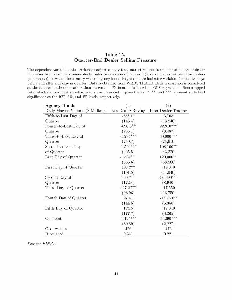
Table 15.Quarter-End Dealer Selling Pressure
The dependent variable is the settlement-adjusted daily total market volume in millions of dollars of dealerpurchases from customers minus dealer sales to customers (column (1)), or of trades between two dealers(column (2)), in which the security was an agency bond. Regressors are indicator variables for the five daysbefore and after a change in quarter. Data is obtained from WRDS TRACE. Each transaction is consideredat the date of settlement rather than execution. Estimation is based on OLS regression. Bootstrappedheteroskedasticity-robust standard errors are presented in parentheses. *, **, and *** represent statisticalsignificance at the 10%, 5%, and 1% levels, respectively.
Agency Bonds (1) (2)Daily Market Volume ($ Millions) Net Dealer Buying Inter-Dealer TradingFifth-to-Last Day of -253.1* 3,708Quarter (146.4) (13,840)Fourth-to-Last Day of -598.8** 22,810***Quarter (236.1) (8,487)Third-to-Last Day of -1,294*** 80,000***Quarter (259.7) (25,610)Second-to-Last Day -1,520*** 108,100**of Quarter (425.5) (43,220)Last Day of Quarter -1,534*** 129,000**
(556.6) (63,860)First Day of Quarter 408.2** -19,070
(191.5) (14,940)Second Day of 366.7** -30,890***Quarter (172.4) (8,940)Third Day of Quarter 427.2*** -17,550
(98.96) (16,750)Fourth Day of Quarter 97.41 -16,260**
(144.5) (6,358)Fifth Day of Quarter 124.5 -12,040
(177.7) (8,265)Constant -1,125*** 64,290***
(30.89) (2,227)Observations 476 476R-squared 0.341 0.221
Source: FINRA
41
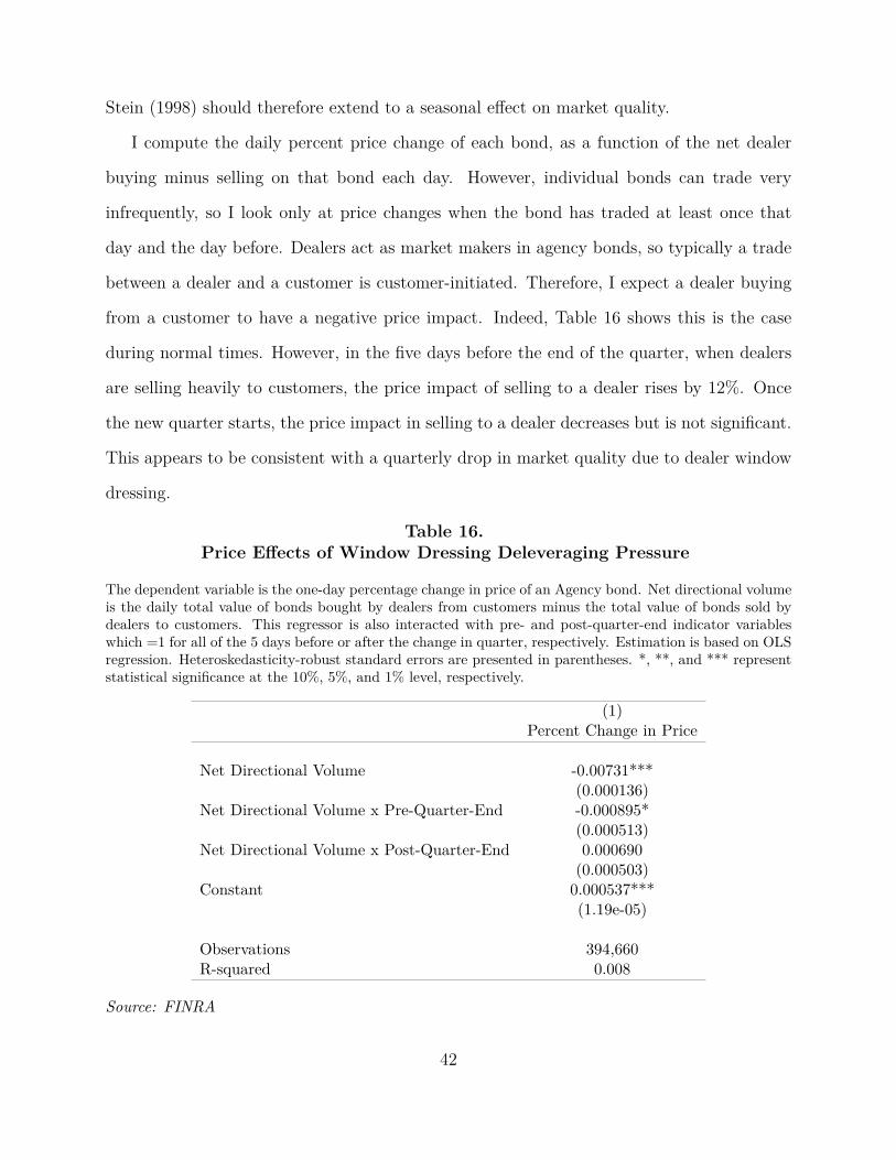
Stein (1998) should therefore extend to a seasonal effect on market quality.
I compute the daily percent price change of each bond, as a function of the net dealer
buying minus selling on that bond each day. However, individual bonds can trade very
infrequently, so I look only at price changes when the bond has traded at least once that
day and the day before. Dealers act as market makers in agency bonds, so typically a trade
between a dealer and a customer is customer-initiated. Therefore, I expect a dealer buying
from a customer to have a negative price impact. Indeed, Table 16 shows this is the case
during normal times. However, in the five days before the end of the quarter, when dealers
are selling heavily to customers, the price impact of selling to a dealer rises by 12%. Once
the new quarter starts, the price impact in selling to a dealer decreases but is not significant.
This appears to be consistent with a quarterly drop in market quality due to dealer window
dressing.
Table 16.Price Effects of Window Dressing Deleveraging Pressure
The dependent variable is the one-day percentage change in price of an Agency bond. Net directional volumeis the daily total value of bonds bought by dealers from customers minus the total value of bonds sold bydealers to customers. This regressor is also interacted with pre- and post-quarter-end indicator variableswhich =1 for all of the 5 days before or after the change in quarter, respectively. Estimation is based on OLSregression. Heteroskedasticity-robust standard errors are presented in parentheses. *, **, and *** representstatistical significance at the 10%, 5%, and 1% level, respectively.
(1)Percent Change in Price
Net Directional Volume -0.00731***(0.000136)
Net Directional Volume x Pre-Quarter-End -0.000895*(0.000513)
Net Directional Volume x Post-Quarter-End 0.000690(0.000503)
Constant 0.000537***(1.19e-05)
Observations 394,660R-squared 0.008
Source: FINRA
42
6.2 Money Market Mutual Funds
Agency bond markets see dealers selling assets for cash, but as shown earlier, money market
funds have a surplus of quarter-end cash. Due to regulatory restrictions, money market
funds cannot invest in long-dated securities such as agency bonds, so there is effectively a
dislocation of cash in the markets each quarter. Repo is a conduit for short-term money to
finance longer-term investments, and quarterly window dressing is a regular stress on this
conduit. Money market funds have had to play a quarterly game of musical chairs to find
short-term assets that they can roll out of when repo resumes at the start of the quarter. The
Federal Reserve’s reverse repurchase agreement program (RRP) was instituted in September
2013, and it appears to be facilitating this process.
In the current zero-interest-rate policy environment, the Fed funds market has become
relatively inactive,19 and the RRP was originally proposed as a new tool to impose a floor
in interest rates by raising the repo rate. To do this, the Federal Reserve will lend collateral
to cash suppliers (mostly money market funds), in essentially a tri-party repo transaction in
which the Fed is the dealer.
Each quarter, the Federal Reserve has increased the amount of collateral it is willing to
repo. Figure 5 shows that at the end of each quarter, cash from money funds surges into
the RRP and immediately flows back out. On September 19, 2014, the Federal Reserve
announced20 (perhaps in an effort to make money funds less reliant on the Federal Reserve
to help cope with window dressing) it would lower the cap on its reverse repo transactions
to $300 billion, which sent rates on ultra-low Treasury bills maturing October 2 below zero.
The RRP was intended to be a tool for raising interest rates by pulling cash out of the money
markets, but at the end of the quarter, it seems the RRP is being overwhelmed by window
dressing.19Afonso, Entz, and LeSueur (2013) online: http://libertystreeteconomics.newyorkfed.org/2013/12/
whos-lending-in-the-fed-funds-market.html20http://online.wsj.com/articles/fed-rate-hike-tool-stirs-some-concern-1411164329
43
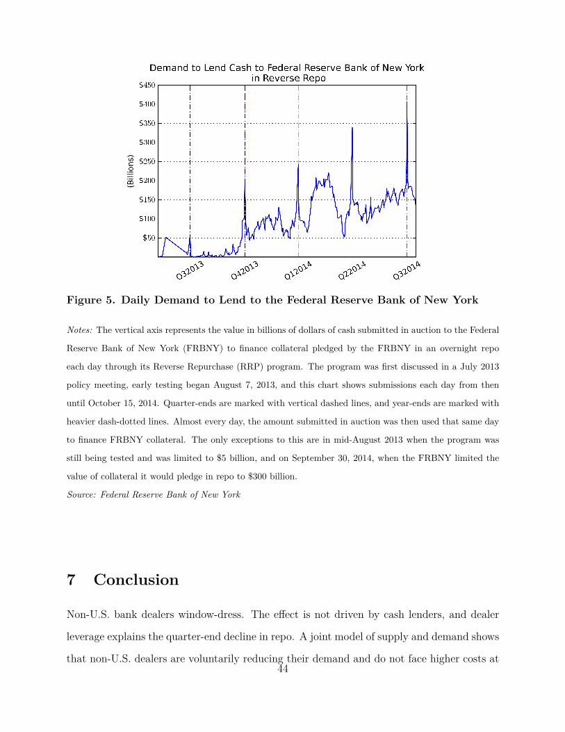
Figure 5. Daily Demand to Lend to the Federal Reserve Bank of New York
Notes: The vertical axis represents the value in billions of dollars of cash submitted in auction to the Federal
Reserve Bank of New York (FRBNY) to finance collateral pledged by the FRBNY in an overnight repo
each day through its Reverse Repurchase (RRP) program. The program was first discussed in a July 2013
policy meeting, early testing began August 7, 2013, and this chart shows submissions each day from then
until October 15, 2014. Quarter-ends are marked with vertical dashed lines, and year-ends are marked with
heavier dash-dotted lines. Almost every day, the amount submitted in auction was then used that same day
to finance FRBNY collateral. The only exceptions to this are in mid-August 2013 when the program was
still being tested and was limited to $5 billion, and on September 30, 2014, when the FRBNY limited the
value of collateral it would pledge in repo to $300 billion.
Source: Federal Reserve Bank of New York
7 Conclusion
Non-U.S. bank dealers window-dress. The effect is not driven by cash lenders, and dealer
leverage explains the quarter-end decline in repo. A joint model of supply and demand shows
that non-U.S. dealers are voluntarily reducing their demand and do not face higher costs at44
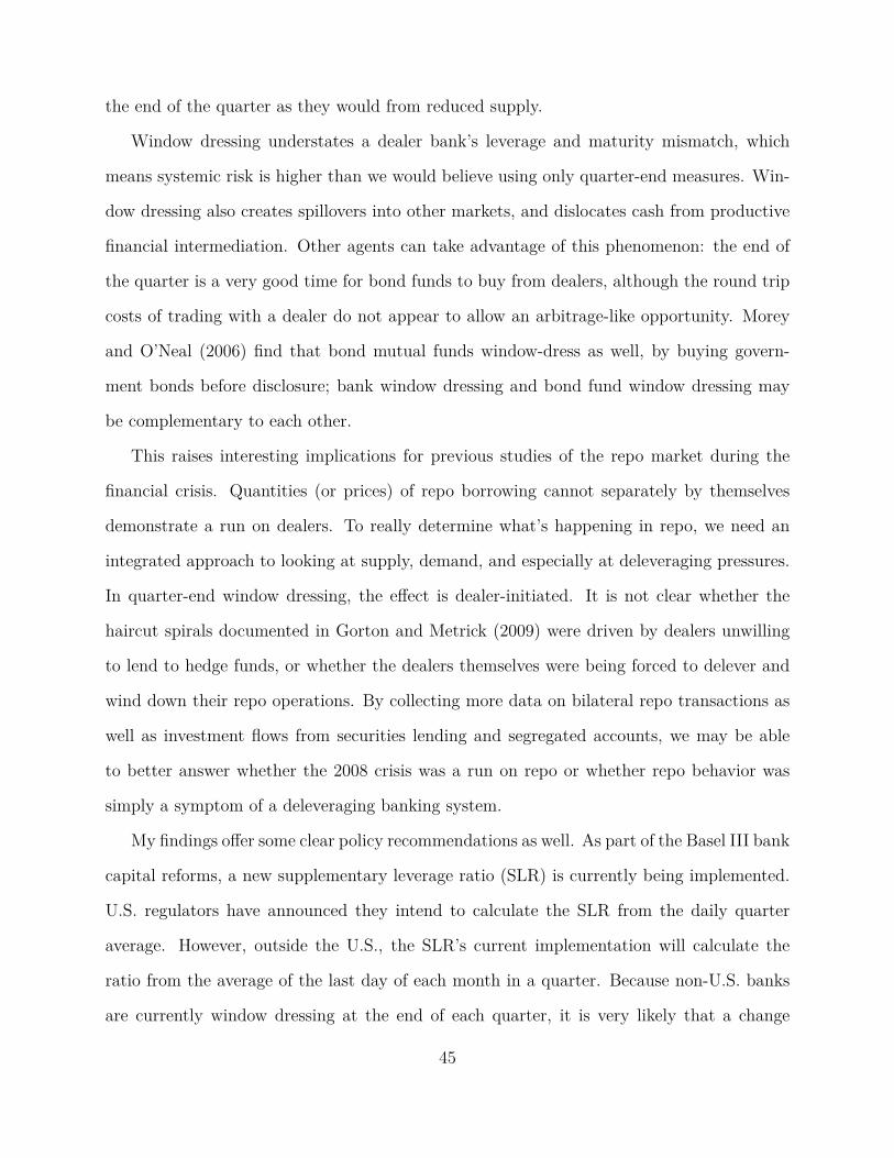
the end of the quarter as they would from reduced supply.
Window dressing understates a dealer bank’s leverage and maturity mismatch, which
means systemic risk is higher than we would believe using only quarter-end measures. Win-
dow dressing also creates spillovers into other markets, and dislocates cash from productive
financial intermediation. Other agents can take advantage of this phenomenon: the end of
the quarter is a very good time for bond funds to buy from dealers, although the round trip
costs of trading with a dealer do not appear to allow an arbitrage-like opportunity. Morey
and O’Neal (2006) find that bond mutual funds window-dress as well, by buying govern-
ment bonds before disclosure; bank window dressing and bond fund window dressing may
be complementary to each other.
This raises interesting implications for previous studies of the repo market during the
financial crisis. Quantities (or prices) of repo borrowing cannot separately by themselves
demonstrate a run on dealers. To really determine what’s happening in repo, we need an
integrated approach to looking at supply, demand, and especially at deleveraging pressures.
In quarter-end window dressing, the effect is dealer-initiated. It is not clear whether the
haircut spirals documented in Gorton and Metrick (2009) were driven by dealers unwilling
to lend to hedge funds, or whether the dealers themselves were being forced to delever and
wind down their repo operations. By collecting more data on bilateral repo transactions as
well as investment flows from securities lending and segregated accounts, we may be able
to better answer whether the 2008 crisis was a run on repo or whether repo behavior was
simply a symptom of a deleveraging banking system.
My findings offer some clear policy recommendations as well. As part of the Basel III bank
capital reforms, a new supplementary leverage ratio (SLR) is currently being implemented.
U.S. regulators have announced they intend to calculate the SLR from the daily quarter
average. However, outside the U.S., the SLR’s current implementation will calculate the
ratio from the average of the last day of each month in a quarter. Because non-U.S. banks
are currently window dressing at the end of each quarter, it is very likely that a change
45
to using month-ends for capital regulation will simply increase the frequency of window
dressing, with commensurate challenges for money market funds and other repo lenders.
In other words, the frequency of reporting a regulatory ratio may matter as much as the
required level of the ratio itself. Of course, Tier 1 and other regulatory ratios would also be
more informative outside the U.S. if foreign banks switched to a quarter-average calculation
as well.
SLR should be quarter-average, all capital requirements should be quarter-average. Fitch
Ratings has claimed that making SLR a daily average instead of month-end average repre-
sents a concession to U.S. custodian banks.21 However, this paper suggests that the opposite
is true. Daily averaging of capital requirements disincentivizes window dressing, which im-
proves the effectiveness of bank regulation.
The RRP appears to be absorbing significant cash each quarter-end that arrives due
to window dressing. The RRP was intended to be a tool for increasing interest rates as
an alternative to fed funds.22 However, the September 17, 2014, announcement capping
the RRP at $300 billion sent money market investors scrambling for alternative short-term
investments for their anticipated excess cash from repo, and dropped yields on short-term
Treasury bills into negative territory. By providing cash lenders with a safe repo counterparty
when others window-dress, the Federal Reserve may be making those lenders dependent on
the RRP at quarter-ends. If window dressing is not fixed, the Fed can at least modify the
RRP to make it flexible during the quarter, increasing the amount of collateral financed at
quarter-end to absorb the surge in cash, but then lowering it during the quarter to match
the decrease in uninvested cash. The recent addition of term repurchase agreements to the
RRP is likely effective in ameliorating this problem.
21Custodian banks are typically cash-rich banks, as opposed to most cash-poor dealer banks. https://www.fitchratings.com/gws/en/fitchwire/fitchwirearticle/US-Leverage-Rule .
22http://www.newyorkfed.org/markets/rrp_faq.html .46
Bibliography
Acharya, Viral, Robert Engle, and Matthew Richardson. “Capital shortfall: A new approach
to ranking and regulating systemic risks.” The American Economic Review 102.3 (2012): 59-
64.
Acharya, Viral V., et al. “Measuring systemic risk.” Social Science Research Network
(2010).
Adrian, Tobias, and Markus K. Brunnermeier.“CoVaR.” No. w17454. National Bureau
of Economic Research, 2011.
Agrawal, Anup, and Kishore Tandon. “Anomalies or illusions? Evidence from stock
markets in eighteen countries.” Journal of international Money and Finance 13.1 (1994):
83-106.
Allen, Franklin, and Douglas Gale. “Limited market participation and volatility of asset
prices.” The American Economic Review (1994): 933-955.
Allen, Linda, and Anthony Saunders. “Bank window dressing: Theory and evidence.”
Journal of Banking & Finance 16.3 (1992): 585-623.
Brockman, Paul, Xiumin Martin, and Emre Unlu. “Executive compensation and the
maturity structure of corporate debt.” The Journal of Finance 65.3 (2010): 1123-1161.
Brownlees, Christian T., and Robert F. Engle. “Volatility, correlation and tails for sys-
temic risk measurement.” Social Science Research Network (2012).
Chernenko, Sergey, and Adi Sunderam. “Frictions in Shadow Banking: Evidence from
the Lending Behavior of Money Market Funds.” Review of Financial Studies, June 2014,
27(6): 1717-1750.
Constantinides, George M. “Optimal stock trading with personal taxes: Implications for
prices and the abnormal January returns.” Journal of Financial Economics 13.1 (1984):
65-89.
Copeland, Adam, Antoine Martin, and Michael Walker.“Repo run: evidence from the
tri-party repo market.” No. 506. Staff Report, Federal Reserve Bank of New York, 2011.47
Diamond, Douglas W., and Philip H. Dybvig. “Bank runs, deposit insurance, and liq-
uidity.” The journal of political economy (1983): 401-419.
Downing, Jeff. “Banks and Balance-Sheet Management: Window-Dressing by Large
Banks.” (2012).
Duffie, Darrell. “Special repo rates.” The Journal of Finance 51.2 (1996): 493-526.
Froot, Kenneth A., David S. Scharfstein, and Jeremy C. Stein. “Risk management:
Coordinating corporate investment and financing policies.” the Journal of Finance 48.5
(1993): 1629-1658.
Froot, Kenneth A., and Jeremy C. Stein. “Risk management, capital budgeting, and cap-
ital structure policy for financial institutions: an integrated approach.” Journal of Financial
Economics 47.1 (1998): 55-82.
Gorton, Gary, and Andrew Metrick. “The Run on Repo and the Panic of 2007-2008.”
Unpublished paper, Yale University (2009).
Gorton, Gary, and Andrew Metrick. “Securitized banking and the run on repo.” Journal
of Financial Economics 104.3 (2012): 425-451.
Gorton, Gary B., and Andrew Metrick. “Who Ran on Repo?” No. w18455. National
Bureau of Economic Research, 2012.
Griffiths, Mark D., and Robert White. 1993. “Tax induced trading and the turn-of-the-
year anomaly: An intraday study.” Journal of Finance 48:575-98.
Griffiths, Mark D., and Drew B. Winters. 1997. “On a preferred habitat for liquidity at
the turn-of-the-year: Evidence from the term repo market.” Journal of Financial Services
Research 12, no.1:21-38.
Griffiths, Mark D., and Drew B. Winters. “The Turn of the Year in Money Markets: Tests
of the Risk-Shifting Window Dressing and Preferred Habitat Hypotheses.” The Journal of
Business 78.4 (2005): 1337-1364.
Haugen, Robert A., and Josef Lakonishok. “The incredible January effect: The stock
market’s unsolved mystery.” Dow Jones-Irwin, 1987.
48
Hu, Grace Xing, Jun Pan, and Jiang Wang. “Tri-Party Repo Pricing.” Available at SSRN
(2014).
Ivashina, Victoria, and David Scharfstein. “Bank lending during the financial crisis of
2008.” Journal of Financial economics 97.3 (2010): 319-338.
Jegadeesh, Narasimhan. “Seasonality in stock price mean reversion: Evidence from the
US and the UK.” The Journal of Finance 46.4 (1991): 1427-1444.
Jordan, Susan D., and Bradford D. Jordan. “Seasonality in daily bond returns.” Journal
of Financial and Quantitative Analysis 26.02 (1991): 269-285.
Keamer, Chaeles. “Macroeconomic seasonality and the January effect.” The Journal of
Finance 49.5 (1994): 1883-1891.
Keim, Donald B. “Size-related anomalies and stock return seasonality: Further empirical
evidence.” Journal of Financial Economics 12.1 (1983): 13-32.
Khwaja, Asim Ijaz, and Atif Mian. “Tracing the impact of bank liquidity shocks: Evi-
dence from an emerging market.” The American Economic Review (2008): 1413-1442.
Koijen, Ralph SJ, and Motohiro Yogo. “Shadow Insurance.” No. w19568. National
Bureau of Economic Research, 2013.
Kotomin, Vladimir, Stanley D. Smith, and Drew B. Winters. “Preferred habitat for
liquidity in international short-term interest rates.” Journal of Banking & Finance 32.2
(2008): 240-250.
Kotomin, Vladimir, and Drew B. Winters. “Quarter-End Effects in Banks: Preferred
Habitat or Window Dressing?” Journal of Financial Services Research 29.1 (2006): 61-82.
Krishnamurthy, Arvind, Stefan Nagel, and Dmitry Orlov. “Sizing up repo.” The Journal
of Finance (2014).
Lakonishok, Josef, and Seymour Smidt. “Are seasonal anomalies real? A ninety-year
perspective.” Review of Financial Studies 1.4 (1988): 403-425.
Lakonishok, Josef, et al. “Window dressing by pension fund managers.” No. w3617.
National Bureau of Economic Research, 1991.
49
Martin, Antoine, David Skeie, and Ernst-Ludwig Von Thadden. “Repo runs.” Review of
Financial Studies 27.4 (2014): 957-989.
Modigliani, Franco, and Richard Sutch. “Innovations in interest rate policy.” The Amer-
ican Economic Review (1966): 178-197.
Morey, Matthew R., and Edward S. O’Neal. “Window dressing in bond mutual funds.”
Journal of Financial Research 29.3 (2006): 325-347.
Musto, David K. “Portfolio disclosures and year-end price shifts.” The Journal of Finance
52.4 (1997): 1563-1588.
Naik, Narayan Y., and Pradeep K. Yadav. “Risk management with derivatives by dealers
and market quality in government bond markets.” The Journal of Finance 58.5 (2003): 1873-
1904.
Ogden, Joseph P. “The end of the month as a preferred habitat: A test of operational ef-
ficiency in the money market.” Journal of Financial and Quantitative Analysis 22.03 (1987):
329-343.
Ogden, Joseph P. “Turn-of-Month Evaluations of Liquid Profits and Stock Returns: A
Common Explanation for the Monthly and January Effects.” The Journal of Finance 45.4
(1990): 1259-1272.
O’Neal, Edward S. “Window dressing and equity mutual funds.” Babcock Graduate
School of Management working paper (2001).
Owens, Edward L., and Joanna Shuang Wu. “Window Dressing of Short-Term Borrow-
ings.” (2012).
Park, Sang Yong, and Marc R. Reinganum. “The puzzling price behavior of treasury bills
that mature at the turn of calendar months.” Journal of Financial Economics 16.2 (1986):
267-283.
Poterba, James M., and Scott J. Weisbenner. “Capital gains tax rules, tax-loss trading,
and turn-of-the-year returns.” The Journal of Finance 56.1 (2001): 353-368.
Qi, Jianping. “Bank liquidity and stability in an overlapping generations model.” Review
50
of Financial Studies 7.2 (1994): 389-417.
Ritter, Jay R. “The buying and selling behavior of individual investors at the turn of the
year.” The Journal of Finance 43.3 (1988): 701-717.
Rozeff, Michael S., and William R. Kinney Jr. “Capital market seasonality: The case of
stock returns.” Journal of Financial Economics 3.4 (1976): 379-402.
Schneeweis, Thomas, and J. Randall Woolridge. “Capital market seasonality: The case
of bond returns.” Journal of Financial and Quantitative Analysis 14.05 (1979): 939-958.
Sias, Richard W., and Laura T. Starks. “Institutions and Individuals at the Turn-of-the-
Year.” The Journal of Finance 52.4 (1997): 1543-1562.
Smirlock, Michael. “Seasonality and bond market returns.” The Journal of Portfolio
Management 11.3 (1985): 42-44.
Sullivan, Ryan, Allan Timmermann, and Halbert White. “Dangers of data mining: The
case of calendar effects in stock returns.” Journal of Econometrics 105.1 (2001): 249-286.
Wermers, Russ. “Mutual fund herding and the impact on stock prices.” The Journal of
Finance 54.2 (1999): 581-622.
51
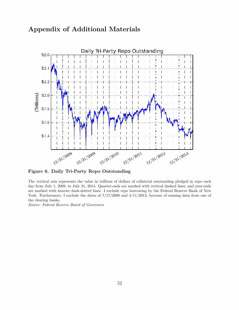
Appendix of Additional Materials
Figure 6. Daily Tri-Party Repo Outstanding
The vertical axis represents the value in trillions of dollars of collateral outstanding pledged in repo eachday from July 1, 2008, to July 31, 2014. Quarter-ends are marked with vertical dashed lines, and year-endsare marked with heavier dash-dotted lines. I exclude repo borrowing by the Federal Reserve Bank of NewYork. Furthermore, I exclude the dates of 7/17/2008 and 4/11/2013, because of missing data from one ofthe clearing banks.Source: Federal Reserve Board of Governors
52
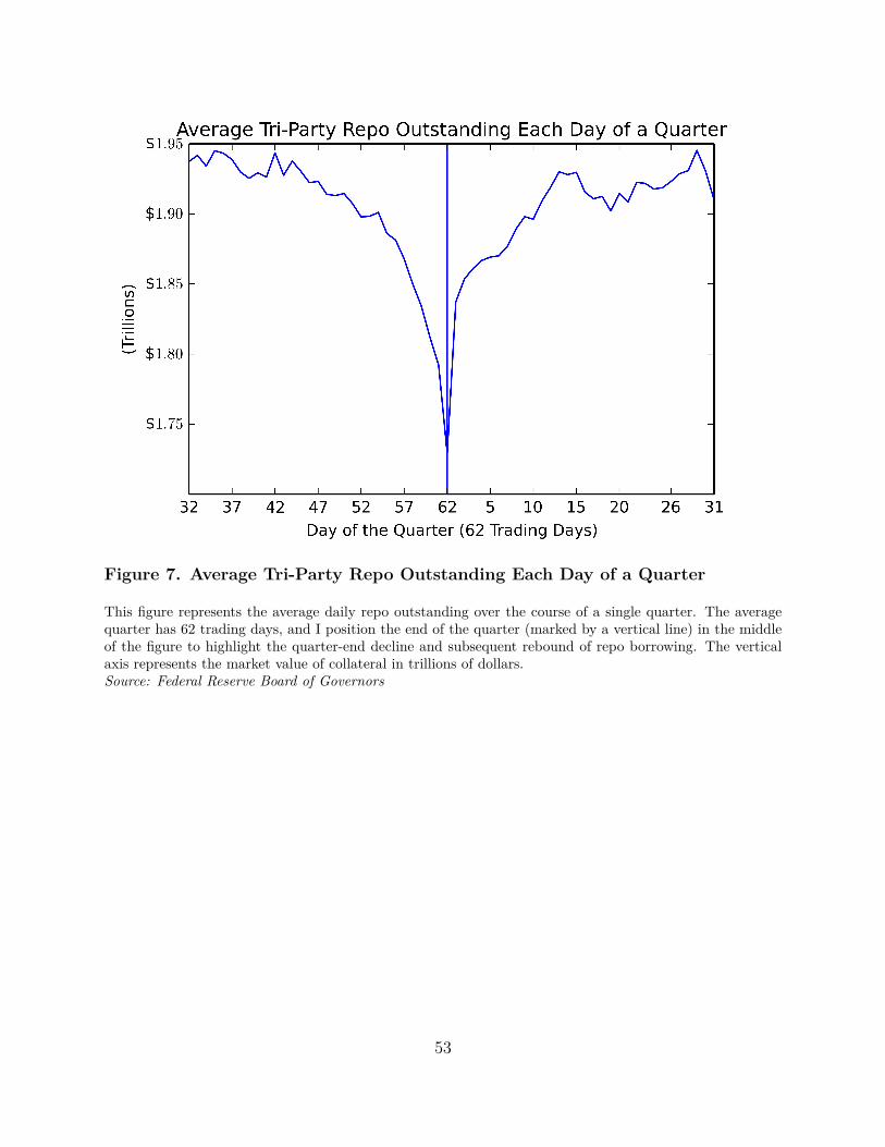
Figure 7. Average Tri-Party Repo Outstanding Each Day of a Quarter
This figure represents the average daily repo outstanding over the course of a single quarter. The averagequarter has 62 trading days, and I position the end of the quarter (marked by a vertical line) in the middleof the figure to highlight the quarter-end decline and subsequent rebound of repo borrowing. The verticalaxis represents the market value of collateral in trillions of dollars.Source: Federal Reserve Board of Governors
53
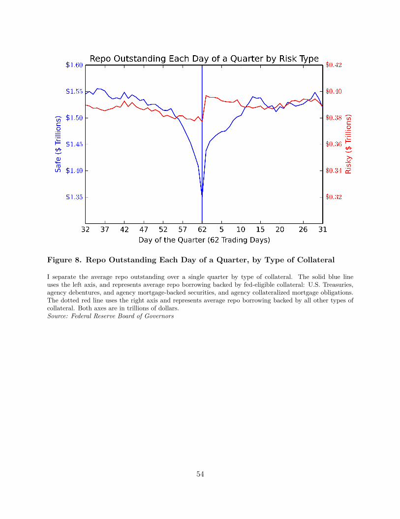
Figure 8. Repo Outstanding Each Day of a Quarter, by Type of Collateral
I separate the average repo outstanding over a single quarter by type of collateral. The solid blue lineuses the left axis, and represents average repo borrowing backed by fed-eligible collateral: U.S. Treasuries,agency debentures, and agency mortgage-backed securities, and agency collateralized mortgage obligations.The dotted red line uses the right axis and represents average repo borrowing backed by all other types ofcollateral. Both axes are in trillions of dollars.Source: Federal Reserve Board of Governors
54
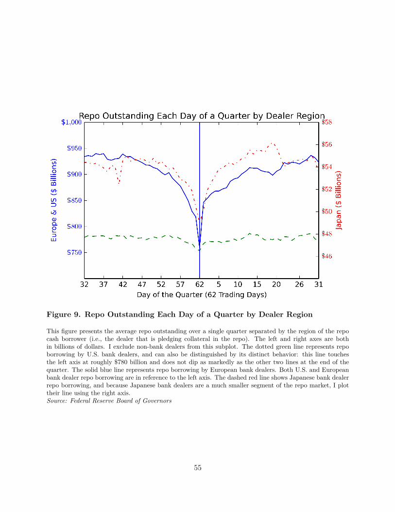
Figure 9. Repo Outstanding Each Day of a Quarter by Dealer Region
This figure presents the average repo outstanding over a single quarter separated by the region of the repocash borrower (i.e., the dealer that is pledging collateral in the repo). The left and right axes are bothin billions of dollars. I exclude non-bank dealers from this subplot. The dotted green line represents repoborrowing by U.S. bank dealers, and can also be distinguished by its distinct behavior: this line touchesthe left axis at roughly $780 billion and does not dip as markedly as the other two lines at the end of thequarter. The solid blue line represents repo borrowing by European bank dealers. Both U.S. and Europeanbank dealer repo borrowing are in reference to the left axis. The dashed red line shows Japanese bank dealerrepo borrowing, and because Japanese bank dealers are a much smaller segment of the repo market, I plottheir line using the right axis.Source: Federal Reserve Board of Governors
55