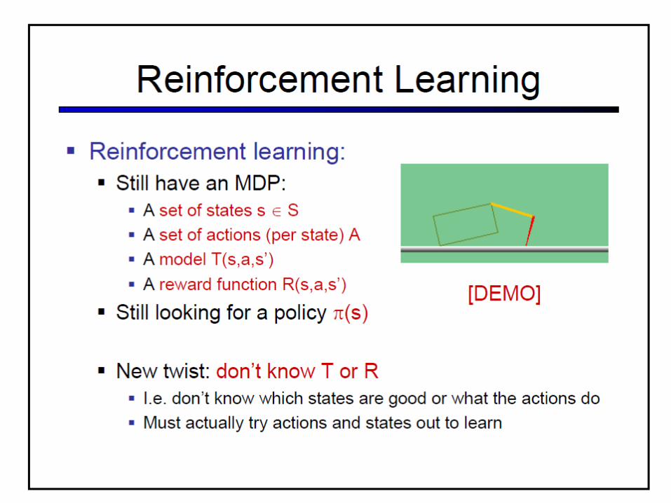
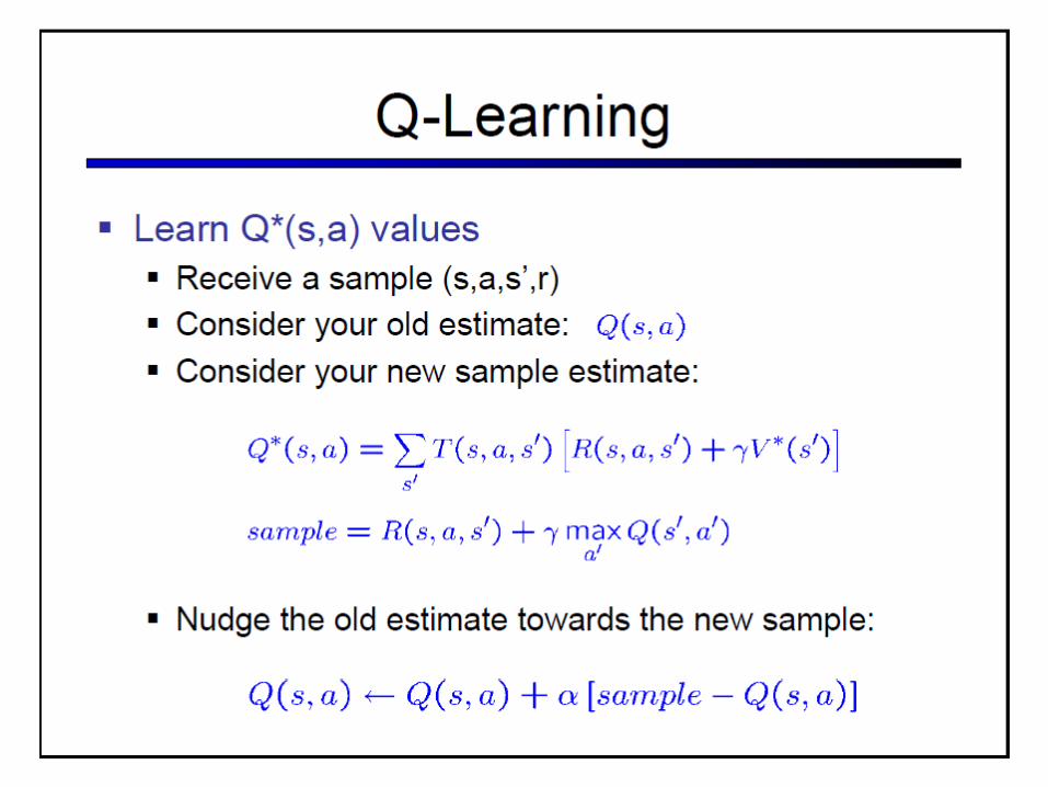
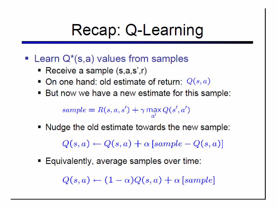
Reinforcement Learning

Slides for this part are adapted from those of Dan Klein@UCB

Main Dimensions

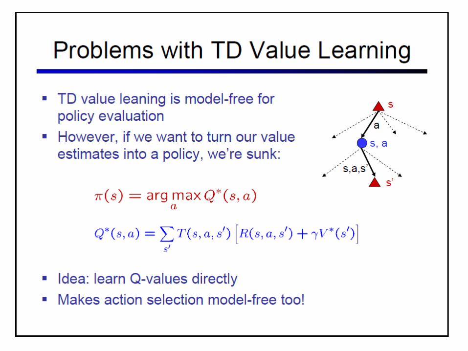
Model-based vs. Model-free• Model-based vs. Model-free

– Model-based Have/learn action models (i.e. transition probabilities)

• Eg. Approximate DP– Model-free Skip them and

directly learn what action to do when (without necessarily finding out the exact model of the action)

• E.g. Q-learning

Passive vs. Active• Passive vs. Active

– Passive: Assume the agent is already following a policy (so there is no action choice to be made; you just need to learn the state values and may be action model)

– Active: Need to learn both the optimal policy and the state values (and may be action model)

Main Dimensions (contd)

Extent of Backup• Full DP

– Adjust value based on values of all the neighbors (as predicted by the transition model)

– Can only be done when transition model is present

• Temporal difference– Adjust value based only on

the actual transitions observed

Does self learning through simulator.[Infants don’t get to “simulate” the world since they neither have T(.) nor R(.) of their world]

We are basically doing EMPIRICAL Policy Evaluation!

But we know this will be wasteful (since it misses the correlation between values of neibhoring states!)

Do DP-based policy evaluation!

10/7

Learning/Planning/Acting

World ---- Model (and Simulator)

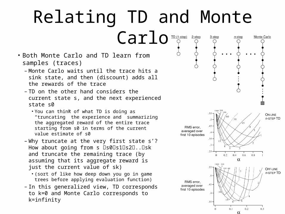
Relating TD and Monte Carlo• Both Monte Carlo and TD learn from samples

(traces)– Monte Carlo waits until the trace hits a sink

state, and then (discount) adds all the rewards of the trace

– TD on the other hand considers the current state s, and the next experienced state s0

• You can think of what TD is doing as “truncating” the experience and summarizing the aggregated reward of the entire trace starting from s0 in terms of the current value estimate of s0

– Why truncate at the very first state s’? How about going from s s0s1s2..sk and truncate the remaining trace (by assuming that its aggregate reward is just the current value of sk)

• (sort of like how deep down you go in game trees before applying evaluation function)

– In this generalized view, TD corresponds to k=0 and Monte Carlo corresponds to k=infinity

Generalizing TD to TD( )l• TD( ) l can be thought of as

doing 1,2…k step predictions of the value of the state, and taking their weighted average

– Weighting is done in terms of l such that

– =0 l corresponds to TD– =1 l corresponds to Monte

Carlo • Note that the last backup

doesn’t have (1- ) l factor…

No (1- ) l factor!

Reason: After Tth state the remaining infinite# states will all havethe same aggregatedBackup—but eachis discounted in l.So, we have a 1/(1- ) l factor that Cancels out the (1- ) l

10/12

Full vs. Partial Backups

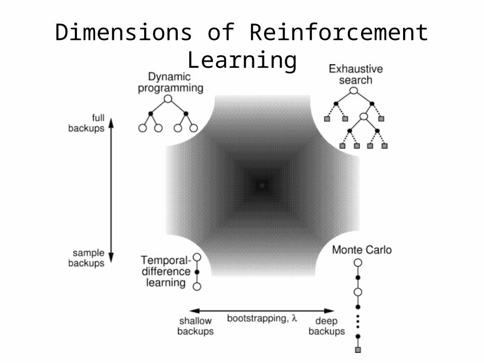
Dimensions of Reinforcement Learning

.

10/14

--Factored TD and Q-learning--Policy search (has to be factored..)

34

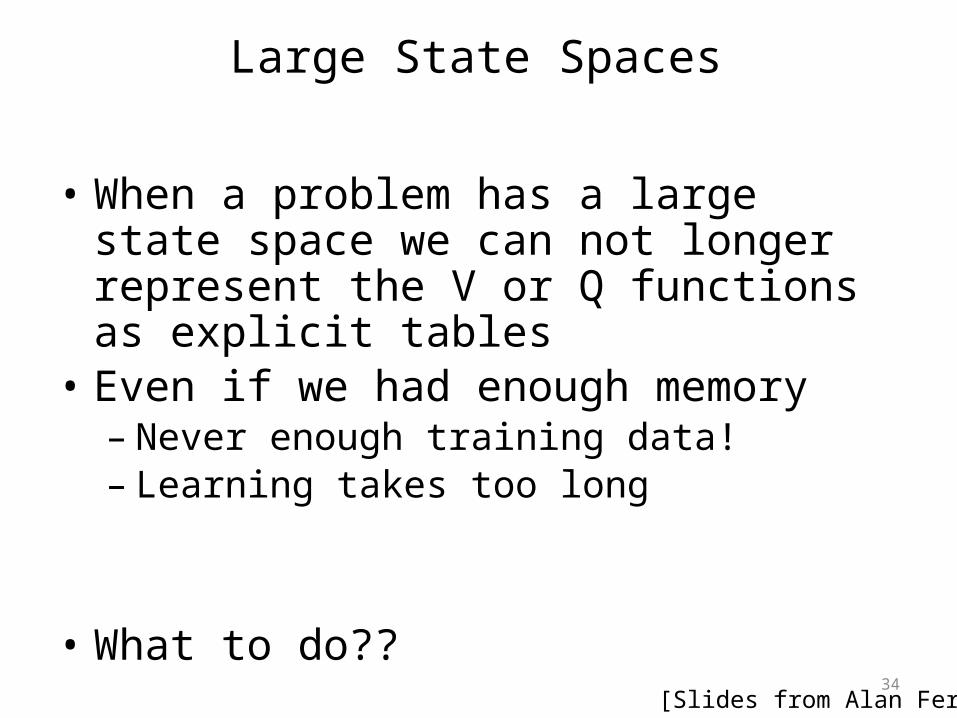
Large State Spaces

• When a problem has a large state space we can not longer represent the V or Q functions as explicit tables

• Even if we had enough memory – Never enough training data!– Learning takes too long

• What to do??

[Slides from Alan Fern]

35

Function Approximation

• Never enough training data!– Must generalize what is learned from one situation to other

“similar” new situations• Idea:

– Instead of using large table to represent V or Q, use a parameterized function

• The number of parameters should be small compared to number of states (generally exponentially fewer parameters)

– Learn parameters from experience– When we update the parameters based on observations in one

state, then our V or Q estimate will also change for other similar states

• I.e. the parameterization facilitates generalization of experience

36

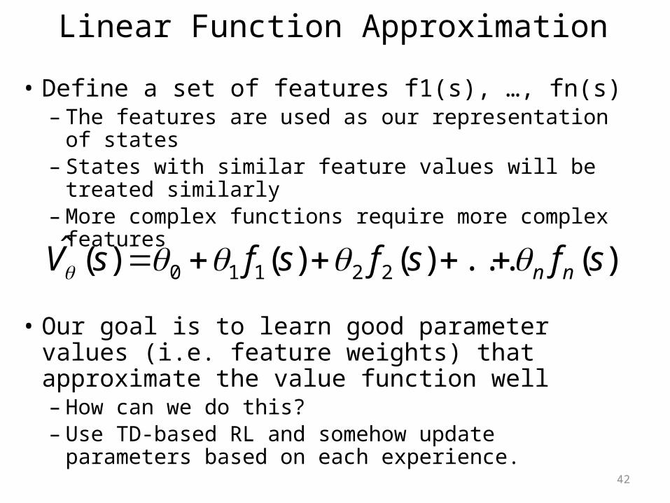
Linear Function Approximation• Define a set of state features f1(s), …, fn(s)

– The features are used as our representation of states– States with similar feature values will be considered to be similar

• A common approximation is to represent V(s) as a weighted sum of the features (i.e. a linear approximation)

• The approximation accuracy is fundamentally limited by the information provided by the features

• Can we always define features that allow for a perfect linear approximation?– Yes. Assign each state an indicator feature. (I.e. i’th feature is 1 iff i’th state

is present and i represents value of i’th state)– Of course this requires far to many features and gives no generalization.

)(...)()()(ˆ 22110 sfsfsfsV nn

37

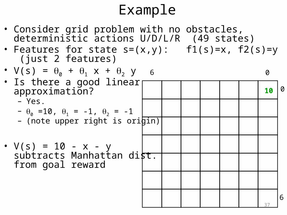
Example• Consider grid problem with no obstacles, deterministic actions

U/D/L/R (49 states)• Features for state s=(x,y): f1(s)=x, f2(s)=y (just 2 features)• V(s) = 0 + 1 x + 2 y• Is there a good linear

approximation?– Yes. – 0 =10, 1 = -1, 2 = -1– (note upper right is origin)

• V(s) = 10 - x - ysubtracts Manhattan dist.from goal reward

10

0

0

6

6

38

But What If We Change Reward …

• V(s) = 0 + 1 x + 2 y• Is there a good linear approximation?

– No.

10

0

0

39

But What If…

• V(s) = 0 + 1 x + 2 y

10

+ 3 z

h Include new feature z5 z= |3-x| + |3-y|

5 z is dist. to goal location

h Does this allow a good linear approx?5 0 =10, 1 = 2 = 0,

0 = -1

0

0

3

3

Feature Engineering….

42

Linear Function Approximation

• Define a set of features f1(s), …, fn(s)– The features are used as our representation of states– States with similar feature values will be treated similarly– More complex functions require more complex features

• Our goal is to learn good parameter values (i.e. feature weights) that approximate the value function well– How can we do this?– Use TD-based RL and somehow update parameters

based on each experience.

)(...)()()(ˆ 22110 sfsfsfsV nn

43

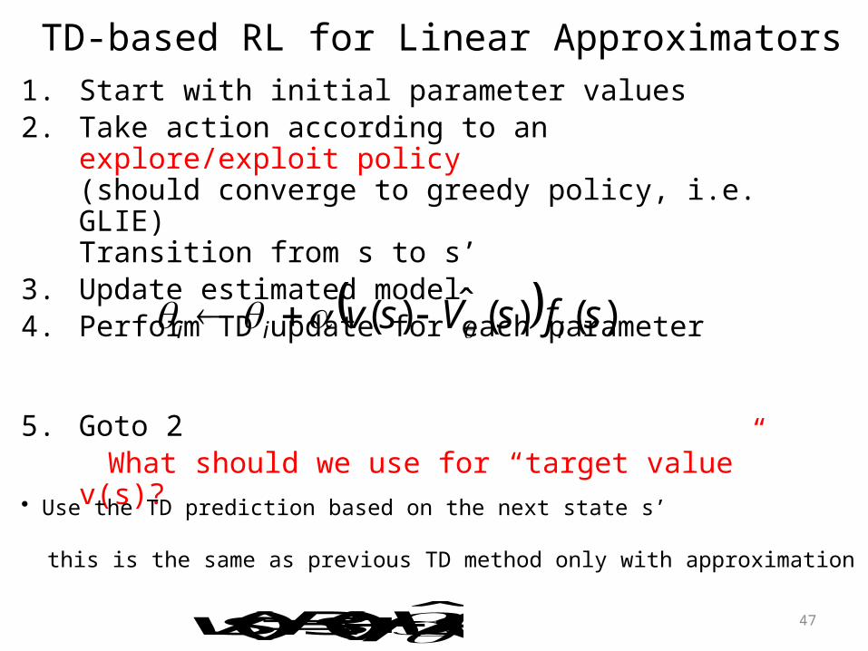
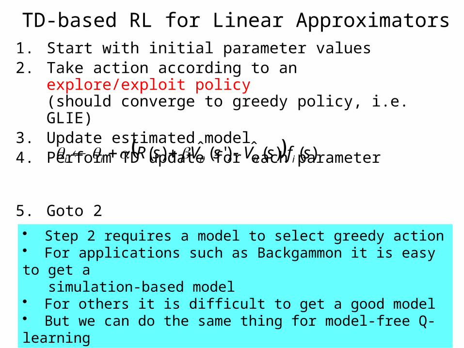
TD-based RL for Linear Approximators

1. Start with initial parameter values2. Take action according to an explore/exploit

policy(should converge to greedy policy, i.e. GLIE)

3. Update estimated model4. Perform TD update for each parameter

5. Goto 2 What is a “TD update” for a parameter?

?i

44

Aside: Gradient Descent• Given a function f(1,…, n) of n real values =(1,…, n) suppose we

want to minimize f with respect to • A common approach to doing this is gradient descent• The gradient of f at point , denoted by f(), is an

n-dimensional vector that points in the direction where f increases most steeply at point

• Vector calculus tells us that f() is just a vector of partial derivatives

where

can decrease f by moving in negative gradient direction

)(),,,,,(lim

)( 111

0

fff niii

i

n

fff

)(,,

)()(

1

45

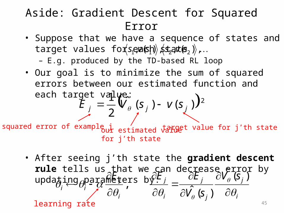
Aside: Gradient Descent for Squared Error

• Suppose that we have a sequence of states and target values for each state– E.g. produced by the TD-based RL loop

• Our goal is to minimize the sum of squared errors between our estimated function and each target value:

• After seeing j’th state the gradient descent rule tells us that we can decrease error by updating parameters by:

2)()(ˆ2

1jjj svsVE

squared error of example j our estimated valuefor j’th state

learning rate

target value for j’th state

i

j

j

j

i

j

i

jii

sV

sV

EEE

)(ˆ

)(ˆ,

,)(,,)(, 2211 svssvs

46

Aside: continued

i

jjji

i

jii

sVsvsV

E

)(ˆ

)()(ˆ

)(ˆ j

j

sV

E

• For a linear approximation function:

• Thus the update becomes:

• For linear functions this update is guaranteed to converge to best approximation for suitable learning rate schedule

)(...)()()(ˆ 22111 sfsfsfsV nn

)()(ˆ)( jijjii sfsVsv

)()(ˆ

jii

j sfsV

depends on form of approximator

47

TD-based RL for Linear Approximators1. Start with initial parameter values2. Take action according to an explore/exploit policy

(should converge to greedy policy, i.e. GLIE) Transition from s to s’

3. Update estimated model4. Perform TD update for each parameter

5. Goto 2 What should we use for “target value” v(s)?

)()(ˆ)( sfsVsv iii

• Use the TD prediction based on the next state s’

this is the same as previous TD method only with approximation

)'(ˆ)()( sVsRsv

48

TD-based RL for Linear Approximators1. Start with initial parameter values2. Take action according to an explore/exploit policy

(should converge to greedy policy, i.e. GLIE) 3. Update estimated model4. Perform TD update for each parameter

5. Goto 2

)()(ˆ)'(ˆ)( sfsVsVsR iii

• Step 2 requires a model to select greedy action • For applications such as Backgammon it is easy to get a simulation-based model • For others it is difficult to get a good model• But we can do the same thing for model-free Q-learning

49

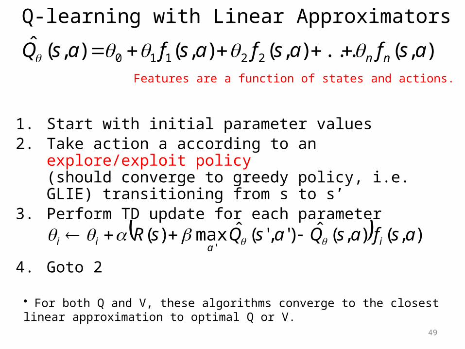
Q-learning with Linear Approximators

1. Start with initial parameter values2. Take action a according to an explore/exploit policy

(should converge to greedy policy, i.e. GLIE) transitioning from s to s’

3. Perform TD update for each parameter

4. Goto 2

),(),(ˆ)','(ˆmax)('

asfasQasQsR ia

ii

),(...),(),(),(ˆ 22110 asfasfasfasQ nn

• For both Q and V, these algorithms converge to the closest linear approximation to optimal Q or V.

Features are a function of states and actions.

57

Policy Gradient Ascent• Let () be the expected value of policy .

– () is just the expected discounted total reward for a trajectory of . – For simplicity assume each trajectory starts at a single initial state.

• Our objective is to find a that maximizes ()

• Policy gradient ascent tells us to iteratively update parameters via:

• Problem: () is generally very complex and it is rare that we

can compute a closed form for the gradient of ().• We will instead estimate the gradient based on experience

)(

58

Gradient Estimation• Concern: Computing or estimating the gradient of

discontinuous functions can be problematic.

• For our example parametric policy

is () continuous? • No.

– There are values of where arbitrarily small changes, cause the policy to change.

– Since different policies can have different values this means that changing can cause discontinuous jump of ().

),(ˆmaxarg)( asQsa

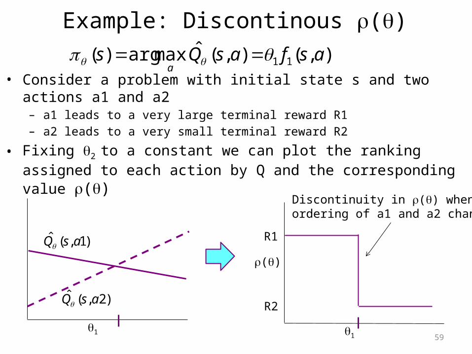
59

Example: Discontinous ()

• Consider a problem with initial state s and two actions a1 and a2 – a1 leads to a very large terminal reward R1 – a2 leads to a very small terminal reward R2

• Fixing 2 to a constant we can plot the ranking assigned to each action by Q and the corresponding value ()

),(),(ˆmaxarg)( 11 asfasQsa

1

)1,(ˆ asQ

)2,(ˆ asQ

1

()

R1

R2

Discontinuity in () when ordering of a1 and a2 change

60

Probabilistic Policies• We would like to avoid policies that drastically change with small

parameter changes, leading to discontinuities• A probabilistic policy takes a state as input and returns a

distribution over actions – Given a state s (s,a) returns the probability that selects action a in s

• Note that () is still well defined for probabilistic policies– Now uncertainty of trajectories comes from environment and policy– Importantly if (s,a) is continuous relative to changing then () is also continuous relative

to changing

• A common form for probabilistic policies is the softmax function or Boltzmann exploration function

Aa

asQ

asQsaas

'

)',(ˆexp

),(ˆexp)|Pr(),(

61

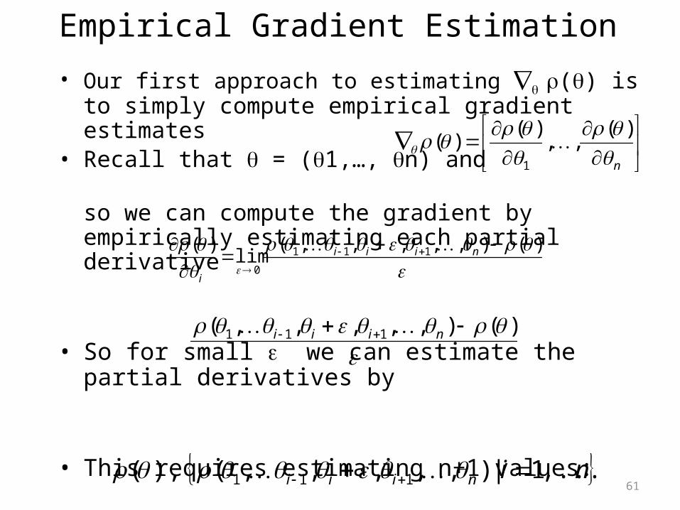
Empirical Gradient Estimation• Our first approach to estimating () is to simply compute

empirical gradient estimates• Recall that = (1,…, n) and

so we can compute the gradient by empirically estimating each partial derivative

• So for small we can estimate the partial derivatives by

• This requires estimating n+1 values:

)(),,,,,(lim

)( 111

0

niii

i

n

)(,,

)()(

1

)(),,,,,( 111 niii

niniii ,...,1|),,,,,(),( 111

62

Empirical Gradient Estimation• How do we estimate the quantities

• For each set of parameters, simply execute the policy for N trials/episodes and average the values achieved across the trials

• This requires a total of N(n+1) episodes to get gradient estimate– For stochastic environments and policies the value of N must be relatively

large to get good estimates of the true value– Often we want to use a relatively large number of parameters– Often it is expensive to run episodes of the policy

• So while this can work well in many situations, it is often not a practical approach computationally

• Better approaches try to use the fact that the stochastic policy is differentiable.

niniii ,...,1|),,,,,(),( 111

64

Policy Gradient Recap• When policies have much simpler representations than

the corresponding value functions, direct search in policy space can be a good idea– Allows us to design complex parametric controllers and optimize details of

parameter settings

• For baseline algorithm the gradient estimates are unbiased (i.e. they will converge to the right value) but have high variance– Can require a large N to get reliable estimates

h OLPOMDP offers can trade-off bias and variance via the discount parameter [Baxter & Bartlett, 2000]

• Can be prone to finding local maxima – Many ways of dealing with this, e.g. random restarts.

65

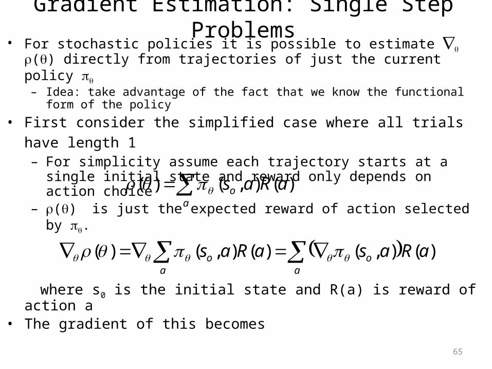
Gradient Estimation: Single Step Problems• For stochastic policies it is possible to estimate () directly from trajectories of

just the current policy – Idea: take advantage of the fact that we know the functional form of the policy

• First consider the simplified case where all trials have length 1 – For simplicity assume each trajectory starts at a single initial state and reward

only depends on action choice– () is just the expected reward of action selected by .

where s0 is the initial state and R(a) is reward of action a• The gradient of this becomes

• How can we estimate this by just observing the execution of ?

a

o aRas )(),()(

a

oa

o aRasaRas )(),()(),()(

66

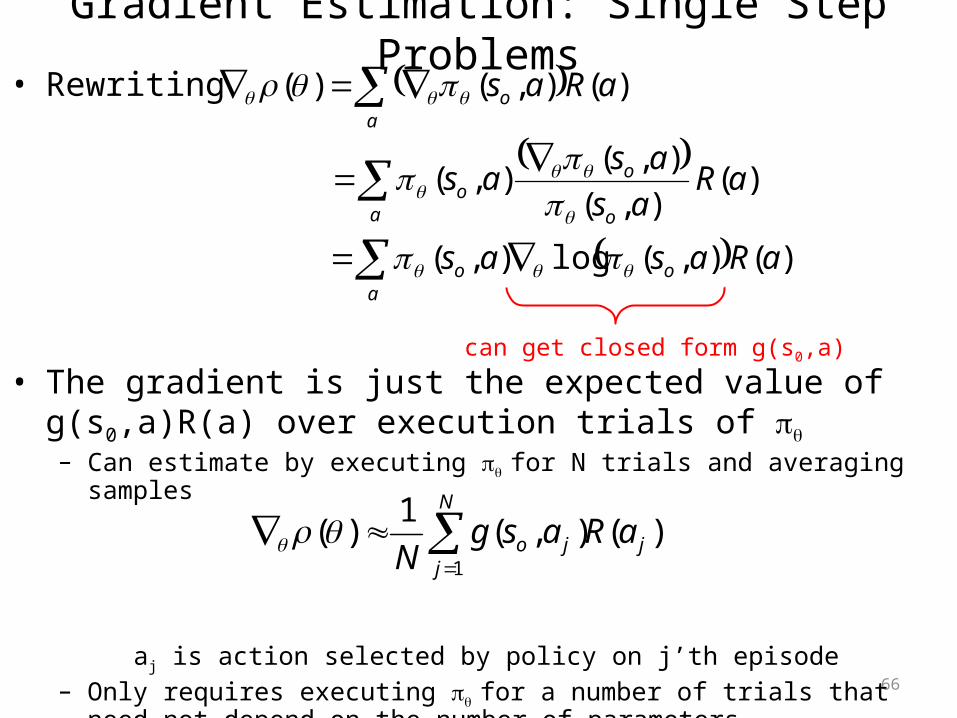
• Rewriting

• The gradient is just the expected value of g(s0,a)R(a) over execution trials of – Can estimate by executing for N trials and averaging samples

aj is action selected by policy on j’th episode – Only requires executing for a number of trials that need not depend on the

number of parameters

aoo

a o

oo

ao

aRasas

aRas

asas

aRas

)(),(log),(

)(),(

),(),(

)(),()(

can get closed form g(s0,a)

)(),(1

)(1

j

N

jjo aRasg

N

Gradient Estimation: Single Step Problems

67

Gradient Estimation: General Case• So for the case of a length 1 trajectories we got:

• For the general case where trajectories have length greater than one and reward depends on state we can do some work and get:

• sjt is t’th state of j’th episode, ajt is t’th action of epidode j• The derivation of this is straightforward but messy.

)(),(1

)(1

aRasgN

N

jjo

N

j

T

ttjjtjtj

j

sRasgN 1 1

,,, )(),(1

)(Observed total reward in trajectory jfrom step t to end

length of trajectory j

# of trajectoriesof current policy

68

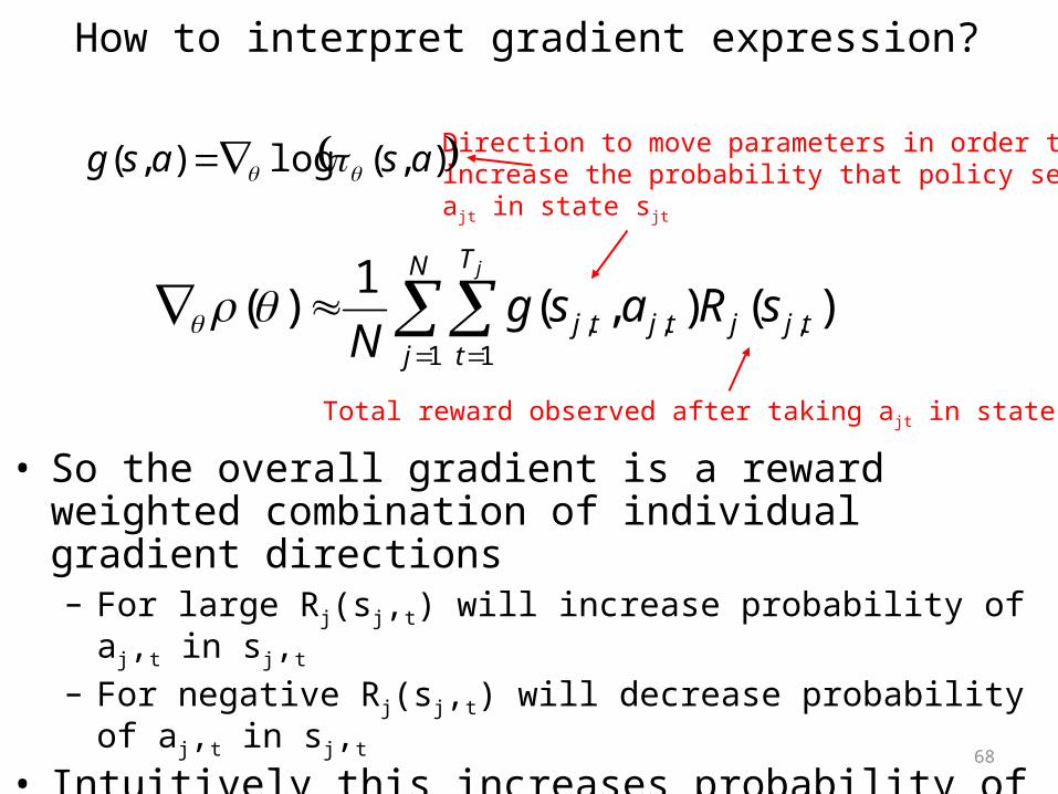
How to interpret gradient expression?

• So the overall gradient is a reward weighted combination of individual gradient directions– For large Rj(sj,t) will increase probability of aj,t in sj,t

– For negative Rj(sj,t) will decrease probability of aj,t in sj,t

• Intuitively this increases probability of taking actions that typically are followed by good reward sequences

N

j

T

ttjjtjtj

j

sRasgN 1 1

,,, )(),(1

)(

Direction to move parameters in order to increase the probability that policy selectsajt in state sjt

Total reward observed after taking ajt in state sjt

),(log),( asasg

69

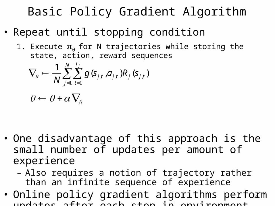
Basic Policy Gradient Algorithm• Repeat until stopping condition

1. Execute for N trajectories while storing the state, action, reward sequences

• One disadvantage of this approach is the small number of updates per amount of experience– Also requires a notion of trajectory rather than an infinite sequence

of experience• Online policy gradient algorithms perform updates after each

step in environment (often learn faster)

N

j

T

ttjjtjtj

j

sRasgN 1 1

,,, )(),(1

72

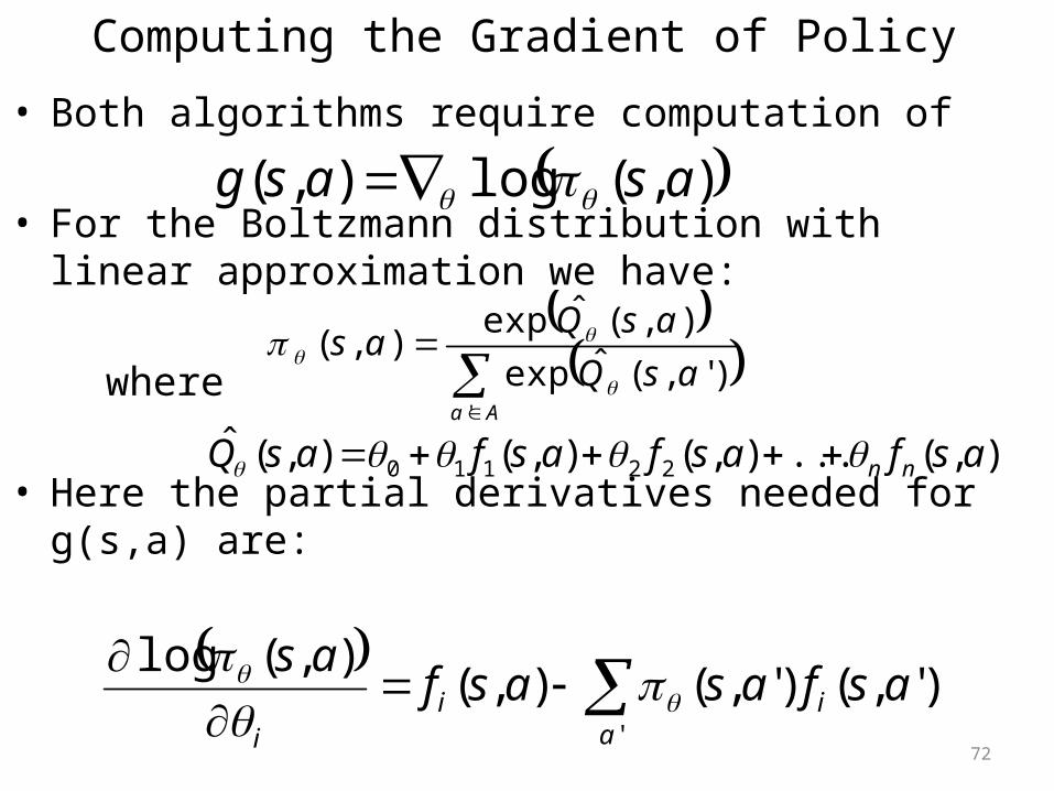
Computing the Gradient of Policy• Both algorithms require computation of

• For the Boltzmann distribution with linear approximation we have:

where

• Here the partial derivatives needed for g(s,a) are:

),(log),( asasg

Aa

asQ

asQas

'

)',(ˆexp

),(ˆexp),(

),(...),(),(),(ˆ 22110 asfasfasfasQ nn

'

)',()',(),(),(log

aii

i

asfasasfas

73

Applications of Policy Gradient Search

• Policy gradient techniques have been used to create controllers for difficult helicopter maneuvers

• For example, inverted helicopter flight.

• A planner called FPG also “won” the 2006 International Planning Competition– If you don’t count FF-Replan