Reinforcing Sampling Distributions through a … Sampling Distributions through a Randomization-Based Activity for Introducing ANOVA . ... Section 2 of this paper provides a literature

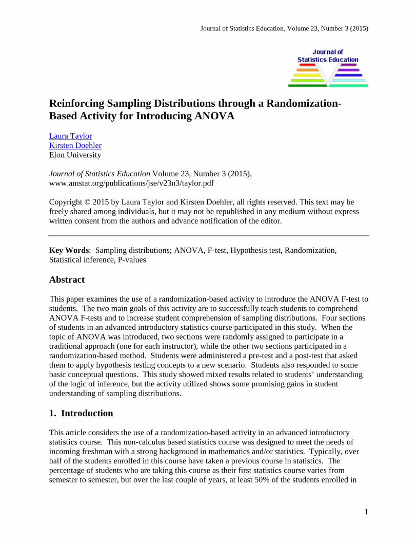
Journal of Statistics Education, Volume 23, Number 3 (2015)

1

Reinforcing Sampling Distributions through a Randomization-Based Activity for Introducing ANOVA Laura Taylor Kirsten Doehler Elon University Journal of Statistics Education Volume 23, Number 3 (2015), www.amstat.org/publications/jse/v23n3/taylor.pdf Copyright © 2015 by Laura Taylor and Kirsten Doehler, all rights reserved. This text may be freely shared among individuals, but it may not be republished in any medium without express written consent from the authors and advance notification of the editor. Key Words: Sampling distributions; ANOVA, F-test, Hypothesis test, Randomization, Statistical inference, P-values Abstract This paper examines the use of a randomization-based activity to introduce the ANOVA F-test to students. The two main goals of this activity are to successfully teach students to comprehend ANOVA F-tests and to increase student comprehension of sampling distributions. Four sections of students in an advanced introductory statistics course participated in this study. When the topic of ANOVA was introduced, two sections were randomly assigned to participate in a traditional approach (one for each instructor), while the other two sections participated in a randomization-based method. Students were administered a pre-test and a post-test that asked them to apply hypothesis testing concepts to a new scenario. Students also responded to some basic conceptual questions. This study showed mixed results related to students’ understanding of the logic of inference, but the activity utilized shows some promising gains in student understanding of sampling distributions. 1. Introduction This article considers the use of a randomization-based activity in an advanced introductory statistics course. This non-calculus based statistics course was designed to meet the needs of incoming freshman with a strong background in mathematics and/or statistics. Typically, over half of the students enrolled in this course have taken a previous course in statistics. The percentage of students who are taking this course as their first statistics course varies from semester to semester, but over the last couple of years, at least 50% of the students enrolled in


2

the course have taken a previous statistics class. In the semester in which the study was performed, 66.7% of participating students had taken a previous statistics course. The advanced introductory course that we teach is very technology heavy, with most calculations being demonstrated once “by-hand” and then repeatedly performed using technology. This class is exclusively taught in a computer lab where students have access to SAS software. As is true for most instructors, our goal is for students to understand the concepts of statistics and then to make appropriate applications. In order to accomplish these goals, we incorporate several randomization-based activities in the course. For instance, we use a modified version of “Example 2: Age Discrimination?” from the document “CIquantresponse.doc” in the 2009 USCOTS Workshop materials of Rossman and Chance (2008) before introducing any formalized hypothesis testing in the course. It has been the experience of the authors that by the midpoint of the semester, students have slipped into a formulaic approach to hypothesis testing whereby they know what curve to draw to calculate p-values, but there is a disconnect between what the curve actually represents (i.e., the distribution of a test statistic under the null hypothesis) and the process of computing the p-value. Thereby, a loss in understanding of why a small p-value indicates evidence against the null hypothesis typically occurs. Most students are generally very good at this point in the semester in recognizing a small p-value as evidence against the null hypothesis and for the alternative hypothesis, but we believe that they no longer truly understand why. To counteract this loss, we have developed a randomization-based activity to introduce ANOVA that focuses on the development of the sampling distribution, which will be the first sampling distribution in class that is right-skewed. The desire is that the randomization process and development of the sampling distribution under random chance will reinforce the definition of a sampling distribution and why sampling distributions are so important in making conclusions related to hypothesis tests. Other objectives of the activity include helping students to understand that some sampling distributions are not symmetric, and the sampling distribution (and shape) are natural occurrences related to the hypothesis testing process. The activity is also meant to reinforce the logic of why a small p-value indicates evidence against the null hypothesis. The activity we have implemented is designed to enforce the GAISE (Guidelines for Assessment and Instruction in Statistics Education) recommendations (Aliaga et al. 2005), particularly recommendations 3 and 4 which are to “Stress conceptual understanding, rather than mere knowledge of procedures” and “Foster active learning in the classroom.” Additionally, we are following the advice in Rossman (2008) to utilize randomization tests to help students to understand the cognitive underpinnings of statistical inference. Section 2 of this paper provides a literature review related to statistics education and specifically to student learning of ANOVA and sampling distributions, the latter of which is often useful to enforce the logic of hypothesis testing. Section 3 discusses the research methodology we have utilized to compare course sections which were taught with either our new activity to introduce ANOVA or a more traditional method of teaching this topic. Details of the randomization activity we generated and its implementation are given in Section 4. The pre-test and post-test


3

assessments that were administered to students are discussed in Section 5, while the corresponding analysis of the responses to the tests are provided in Section 6. There are numerous notes on student responses in both the pre- and post-tests which are mentioned in Section 7. The concluding section of this paper provides recommendations for implementation of the activity and mentions directions for future research. 2. Literature Review 2.1 Teaching ANOVA ANOVA is a challenging topic to cover, especially in an introductory statistics class. A main reason for this is that students must have solid knowledge of numerous mathematical and statistical topics, including, but not limited to, sums of squares, variability, p-values, the F-distribution, and hypotheses (Braun 2012). Previous research studies have investigated different approaches to effectively teach ANOVA (Sturm-Beiss 2005; Lesser and Melgoza 2007; Rossman and Chance 2008; Braun 2012). Both Sturm-Beiss and Rossman and Chance have developed applets for easy visualization of ANOVA. Braun has provided an interesting hands-on activity to introduce ANOVA through an investigation of flight distance by paper airplanes made from paper with one of three different weights. Braun’s method involves computing residuals (original observations minus group average), and generating false data from adding the grand mean to the residuals. Braun then repeated the process of sampling from the simulated data and averaging those observations. Graphs showing both treatment and simulated averages help students in visualization. Lesser and Melgoza discussed an application of a numerical approach for learning ANOVA based on a data set with only three groupings and five observations in each group. Smaller data sets allow for easy computations by hand. We follow the example of Lesser and Melgoza by also utilizing a small data set in our activity. 2.2 Sampling Distributions and the Randomization Approach The idea of a sampling distribution and its use in inferential statistics is also a very challenging topic for students to fully grasp. It has been suggested that students’ understanding of sampling distributions could be improved via computer simulation activities, although even with appropriate software, students may still be under par in their understanding of sampling distributions (delMas, Garfield, and Chance 1999). Pfannkuch (2007) notes that students are often lacking in their awareness of sampling distributions, and this can drastically impede students’ ability to perform statistical inference. Cobb (2007, p. 7) states that “The idea of a sampling distribution is inherently hard for students, in the same way that the idea of a derivative is hard.” Cobb discusses a permutation in a two sample scenario where initial data values are randomly assigned to two groups, a statistic is computed, and the process is repeated. Permutation tests involve randomization, and they are also known as randomization tests. Cobb encourages statistics educators to teach inference using a randomization approach. In his 2007 article, he compares the t-test to a rotary phone and a tape player. In other words, these two things are decreasing in their popularity and becoming less


4

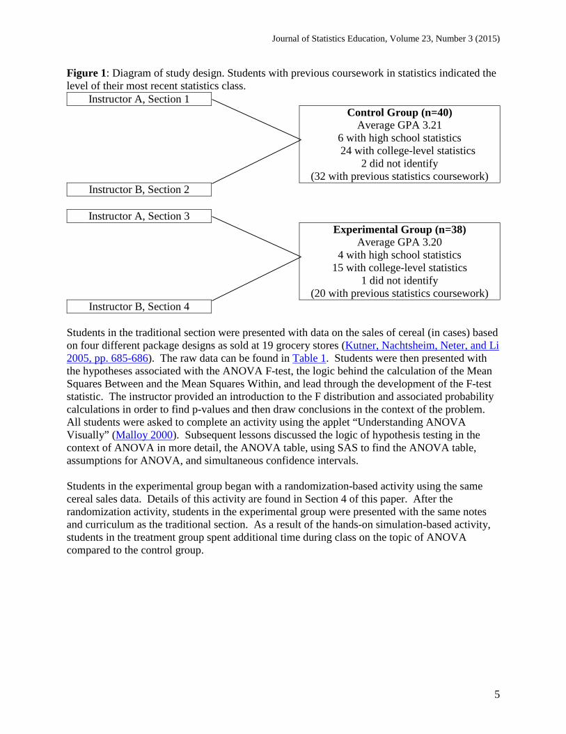
useful today due to vast advancements in technology. Cobb discusses a dozen reasons why a randomization-based curriculum should be used when teaching statistics. The last reason listed is that Sir Ronald Aylmer Fisher (1936) recommended that we utilize permutation methods. Other researchers have also investigated and encouraged the teaching of statistics through randomization-based methods to enforce concepts of sampling distributions and sampling variability (Rossman and Chance 2000; Tintle, VanderStoep, Holmes, Quisenberry, and Swanson 2011; Wild, Pfannkuch, Regan, and Horton 2011). We particularly heed the call of Rossman and Chance (2000) to “Have students perform physical simulations to discover basic ideas of inference.” Rossman and Chance (2014) provide a comprehensive overview of various curriculums, textbooks, software, and NSF funded projects which have helped to encourage and facilitate the teaching of statistical inference with simulation-based approaches. 3. Research Method To test the effectiveness of the simulation-based method to introduce ANOVA versus the traditional approach, each instructor taught two sections of the same advanced introductory course. One section for each professor was randomly assigned to use the traditional ANOVA introduction and one the randomization-based ANOVA introduction. Prior to experimentation, informed consent was collected under IRB approval. Students were administered a pre-test (see Appendix A) prior to instruction. ANOVA was introduced in the assigned format (traditional or randomization-based), and then a post-test (see Appendix B) similar in nature to the pre-test was administered in a following class. Of the 78 students who provided consent and completed both the pre- and post-tests, 40 were in the control group and 38 were in the experimental group. Each section of the course was capped at 30 students, so approximately two-thirds of all students provided consent and completed both tests. Figure 1 depicts the study design. Students provided information on their current GPA and their most recent previous statistics experiences in demographic questions provided as part of the pre-test.


5

Figure 1: Diagram of study design. Students with previous coursework in statistics indicated the level of their most recent statistics class.

Instructor A, Section 1 Control Group (n=40)

Average GPA 3.21 6 with high school statistics

24 with college-level statistics 2 did not identify

(32 with previous statistics coursework) Instructor B, Section 2

Instructor A, Section 3

Experimental Group (n=38) Average GPA 3.20

4 with high school statistics 15 with college-level statistics

1 did not identify (20 with previous statistics coursework)

Instructor B, Section 4 Students in the traditional section were presented with data on the sales of cereal (in cases) based on four different package designs as sold at 19 grocery stores (Kutner, Nachtsheim, Neter, and Li 2005, pp. 685-686). The raw data can be found in Table 1. Students were then presented with the hypotheses associated with the ANOVA F-test, the logic behind the calculation of the Mean Squares Between and the Mean Squares Within, and lead through the development of the F-test statistic. The instructor provided an introduction to the F distribution and associated probability calculations in order to find p-values and then draw conclusions in the context of the problem. All students were asked to complete an activity using the applet “Understanding ANOVA Visually” (Malloy 2000). Subsequent lessons discussed the logic of hypothesis testing in the context of ANOVA in more detail, the ANOVA table, using SAS to find the ANOVA table, assumptions for ANOVA, and simultaneous confidence intervals. Students in the experimental group began with a randomization-based activity using the same cereal sales data. Details of this activity are found in Section 4 of this paper. After the randomization activity, students in the experimental group were presented with the same notes and curriculum as the traditional section. As a result of the hands-on simulation-based activity, students in the treatment group spent additional time during class on the topic of ANOVA compared to the control group.


6

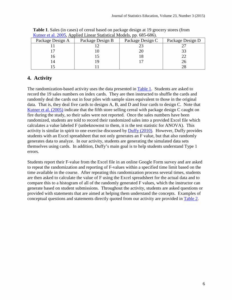
Table 1. Sales (in cases) of cereal based on package design at 19 grocery stores (from Kutner et al. 2005, Applied Linear Statistical Models, pp. 685-686).

Package Design A Package Design B Package Design C Package Design D 11 17 16 14 15

12 10 15 19 11

23 20 18 17

27 33 22 26 28

4. Activity The randomization-based activity uses the data presented in Table 1. Students are asked to record the 19 sales numbers on index cards. They are then instructed to shuffle the cards and randomly deal the cards out in four piles with sample sizes equivalent to those in the original data. That is, they deal five cards to designs A, B, and D and four cards to design C. Note that Kutner et al. (2005) indicate that the fifth store selling cereal with package design C caught on fire during the study, so their sales were not reported. Once the sales numbers have been randomized, students are told to record their randomized sales into a provided Excel file which calculates a value labeled F (unbeknownst to them, it is the test statistic for ANOVA). This activity is similar in spirit to one exercise discussed by Duffy (2010). However, Duffy provides students with an Excel spreadsheet that not only generates an F value, but that also randomly generates data to analyze. In our activity, students are generating the simulated data sets themselves using cards. In addition, Duffy’s main goal is to help students understand Type 1 errors. Students report their F-value from the Excel file in an online Google Form survey and are asked to repeat the randomization and reporting of F-values within a specified time limit based on the time available in the course. After repeating this randomization process several times, students are then asked to calculate the value of F using the Excel spreadsheet for the actual data and to compare this to a histogram of all of the randomly generated F values, which the instructor can generate based on student submissions. Throughout the activity, students are asked questions or provided with statements that are aimed at helping them understand the concepts. Examples of conceptual questions and statements directly quoted from our activity are provided in Table 2.


7

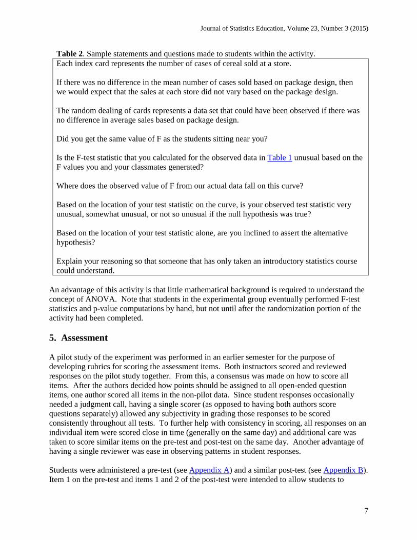
Table 2. Sample statements and questions made to students within the activity. Each index card represents the number of cases of cereal sold at a store. If there was no difference in the mean number of cases sold based on package design, then we would expect that the sales at each store did not vary based on the package design. The random dealing of cards represents a data set that could have been observed if there was no difference in average sales based on package design. Did you get the same value of F as the students sitting near you? Is the F-test statistic that you calculated for the observed data in Table 1 unusual based on the F values you and your classmates generated? Where does the observed value of F from our actual data fall on this curve? Based on the location of your test statistic on the curve, is your observed test statistic very unusual, somewhat unusual, or not so unusual if the null hypothesis was true? Based on the location of your test statistic alone, are you inclined to assert the alternative hypothesis? Explain your reasoning so that someone that has only taken an introductory statistics course could understand.

An advantage of this activity is that little mathematical background is required to understand the concept of ANOVA. Note that students in the experimental group eventually performed F-test statistics and p-value computations by hand, but not until after the randomization portion of the activity had been completed.

5. Assessment A pilot study of the experiment was performed in an earlier semester for the purpose of developing rubrics for scoring the assessment items. Both instructors scored and reviewed responses on the pilot study together. From this, a consensus was made on how to score all items. After the authors decided how points should be assigned to all open-ended question items, one author scored all items in the non-pilot data. Since student responses occasionally needed a judgment call, having a single scorer (as opposed to having both authors score questions separately) allowed any subjectivity in grading those responses to be scored consistently throughout all tests. To further help with consistency in scoring, all responses on an individual item were scored close in time (generally on the same day) and additional care was taken to score similar items on the pre-test and post-test on the same day. Another advantage of having a single reviewer was ease in observing patterns in student responses. Students were administered a pre-test (see Appendix A) and a similar post-test (see Appendix B). Item 1 on the pre-test and items 1 and 2 of the post-test were intended to allow students to


8

demonstrate the mechanics of a hypothesis test in an abstract way and more specifically to present the material to students outside of the context of a sampling distribution with which they were already familiar. The goals of these items were to see if the students could apply their knowledge of hypothesis testing to a new scenario. In order to do this, we employed the following mechanisms:

• We used notation for parameters that they had not seen before. • We used appropriate terminology, such as “test statistic” and “sampling distribution” to

describe the number provided and the graph. • We used a unique and unfamiliar sampling distribution. • We used hypotheses that resembled those from a one-sample hypothesis test.

Student responses on item 1 of the pre-test and items 1 and 2 on the post-test were evaluated based on the following criteria which were each worth one point:

• In part (a), did students correctly locate the test statistic on the sampling distribution? • In part (a), did students shade the curve in the correct direction based on the alternative

hypothesis? • In part (a), did students use the sampling distribution to find the p-value (or did they

incorrectly use the normal or t distribution)? • In part (a), did students discuss the probability as being the area under the curve? • In part (b), did students correctly indicate the size of the p-value (based on their answer to

part (a))? • In part (c), did students indicate that they were looking at the area that was shaded in part

(a)? • In part (c), did students indicate that they made a comparison to the significance level of

0.05?

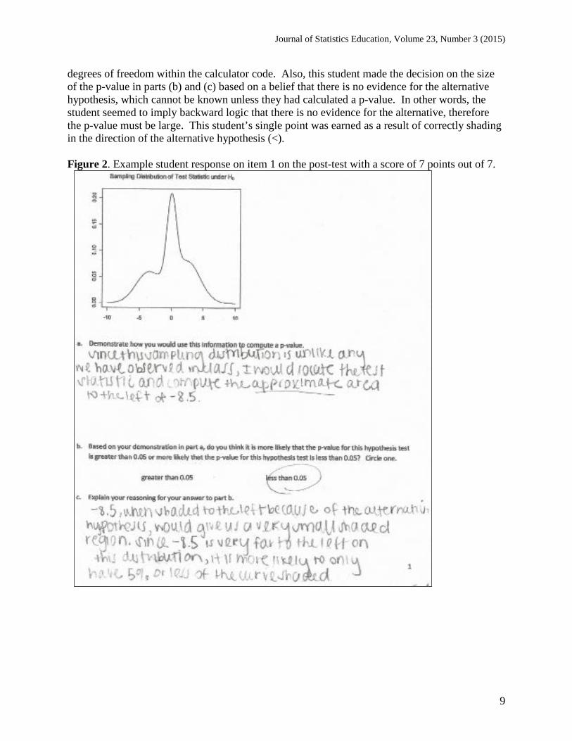
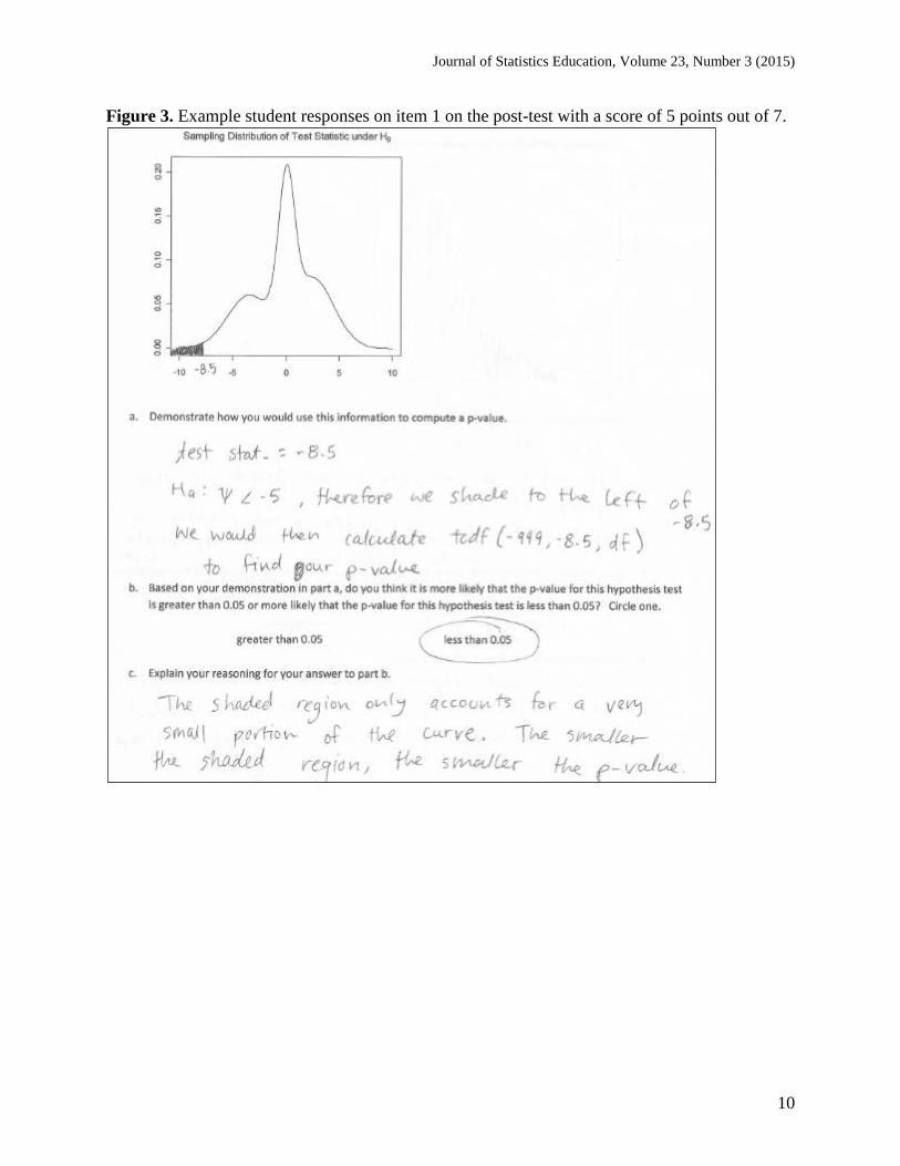
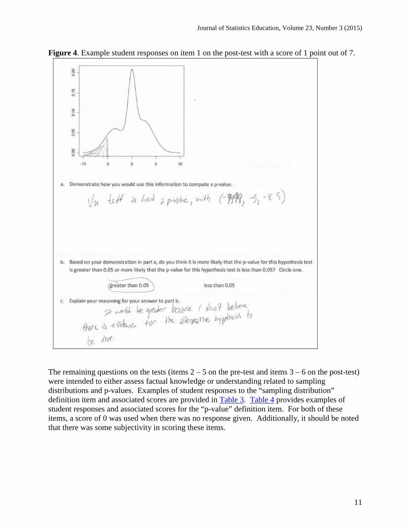
Total scores on item 1 of the pre-test and items 1 and 2 on the post-test were worth seven points. In most places within this article, the average scores on items 1 and 2 of the post-test are reported as a single average score in order to directly compare with item 1 on the pre-test. In other instances, item 1 on the pre-test is compared directly to item 1 on the post-test. Figures 2, 3, and 4 include several examples of student work on these items reflecting scores of 7/7, 5/7, and 1/7, respectively. Figures 2, 3, and 4 show responses from the first question of the post-test. The student response in Figure 2 was scored 7/7 based on the previous bullets: this student located the test statistic (–8.5), shaded in the direction of the alternative hypothesis (<), used the sampling distribution provided (not t, normal, or F), specifically stated that the p-value was the area under the curve, correctly specified the approximate size of the p-value (less than 0.05), and provided an explanation that they were comparing the shaded area of the curve to the significance level of 0.05. In contrast, the student response in Figure 3 indicated that this student would find the area under the curve (which was correctly shaded) using tcdf on the calculator. This implied that this student would use the t-distribution to calculate the probability. In addition, this student did not explicitly state that he or she compared the area of the shaded region to 0.05. For the final student response in Figure 4, this student located the null value on the curve (not the test statistic) and inappropriately implied the use of a t-distribution through the indication of calculator code. This response also incorrectly used the test statistic in place of the


9

degrees of freedom within the calculator code. Also, this student made the decision on the size of the p-value in parts (b) and (c) based on a belief that there is no evidence for the alternative hypothesis, which cannot be known unless they had calculated a p-value. In other words, the student seemed to imply backward logic that there is no evidence for the alternative, therefore the p-value must be large. This student’s single point was earned as a result of correctly shading in the direction of the alternative hypothesis (<). Figure 2. Example student response on item 1 on the post-test with a score of 7 points out of 7.


10

Figure 3. Example student responses on item 1 on the post-test with a score of 5 points out of 7.


11

Figure 4. Example student responses on item 1 on the post-test with a score of 1 point out of 7.

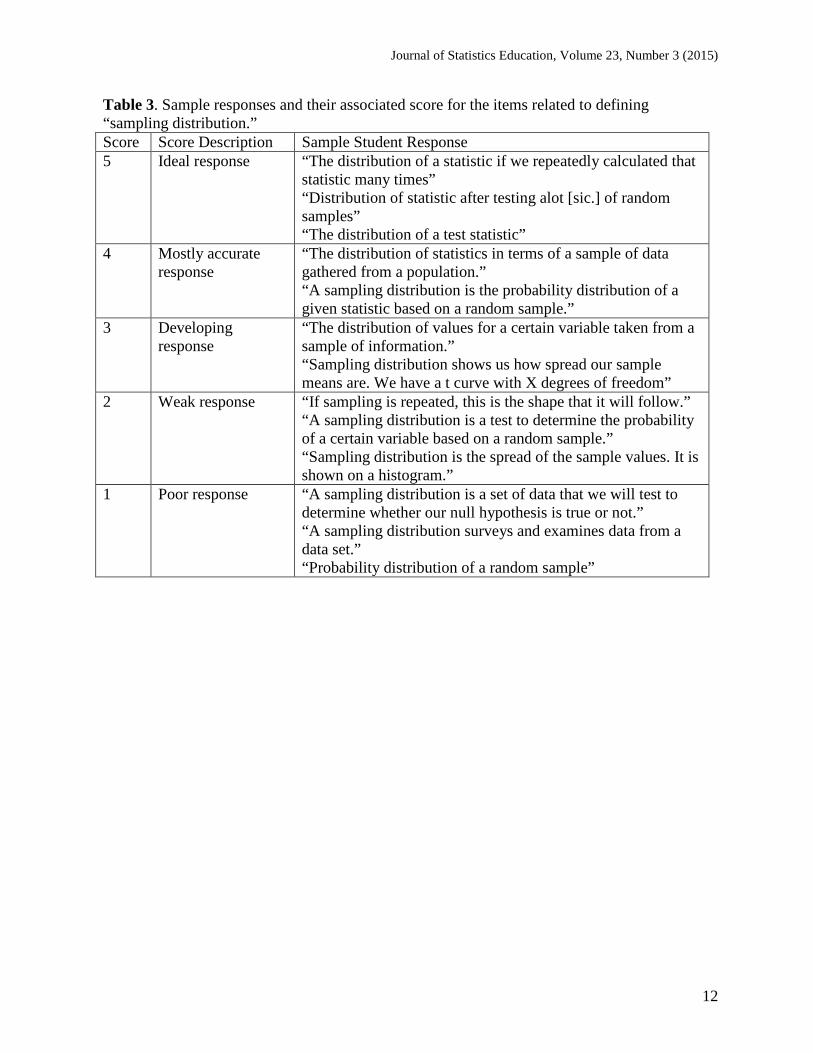
The remaining questions on the tests (items 2 – 5 on the pre-test and items 3 – 6 on the post-test) were intended to either assess factual knowledge or understanding related to sampling distributions and p-values. Examples of student responses to the “sampling distribution” definition item and associated scores are provided in Table 3. Table 4 provides examples of student responses and associated scores for the “p-value” definition item. For both of these items, a score of 0 was used when there was no response given. Additionally, it should be noted that there was some subjectivity in scoring these items.


12

Table 3. Sample responses and their associated score for the items related to defining “sampling distribution.” Score Score Description Sample Student Response 5 Ideal response “The distribution of a statistic if we repeatedly calculated that

statistic many times” “Distribution of statistic after testing alot [sic.] of random samples” “The distribution of a test statistic”

4 Mostly accurate response

“The distribution of statistics in terms of a sample of data gathered from a population.” “A sampling distribution is the probability distribution of a given statistic based on a random sample.”

3 Developing response

“The distribution of values for a certain variable taken from a sample of information.” “Sampling distribution shows us how spread our sample means are. We have a t curve with X degrees of freedom”

2 Weak response “If sampling is repeated, this is the shape that it will follow.” “A sampling distribution is a test to determine the probability of a certain variable based on a random sample.” “Sampling distribution is the spread of the sample values. It is shown on a histogram.”

1 Poor response “A sampling distribution is a set of data that we will test to determine whether our null hypothesis is true or not.” “A sampling distribution surveys and examines data from a data set.” “Probability distribution of a random sample”


13

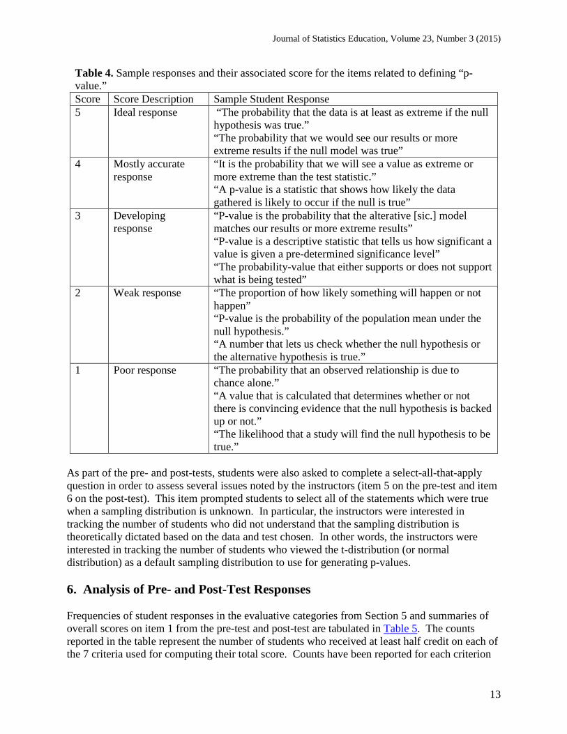
Table 4. Sample responses and their associated score for the items related to defining “p-value.” Score Score Description Sample Student Response 5 Ideal response “The probability that the data is at least as extreme if the null

hypothesis was true.” “The probability that we would see our results or more extreme results if the null model was true”

4 Mostly accurate response

“It is the probability that we will see a value as extreme or more extreme than the test statistic.” “A p-value is a statistic that shows how likely the data gathered is likely to occur if the null is true”

3 Developing response

“P-value is the probability that the alterative [sic.] model matches our results or more extreme results” “P-value is a descriptive statistic that tells us how significant a value is given a pre-determined significance level” “The probability-value that either supports or does not support what is being tested”

2 Weak response “The proportion of how likely something will happen or not happen” “P-value is the probability of the population mean under the null hypothesis.” “A number that lets us check whether the null hypothesis or the alternative hypothesis is true.”

1 Poor response “The probability that an observed relationship is due to chance alone.” “A value that is calculated that determines whether or not there is convincing evidence that the null hypothesis is backed up or not.” “The likelihood that a study will find the null hypothesis to be true.”

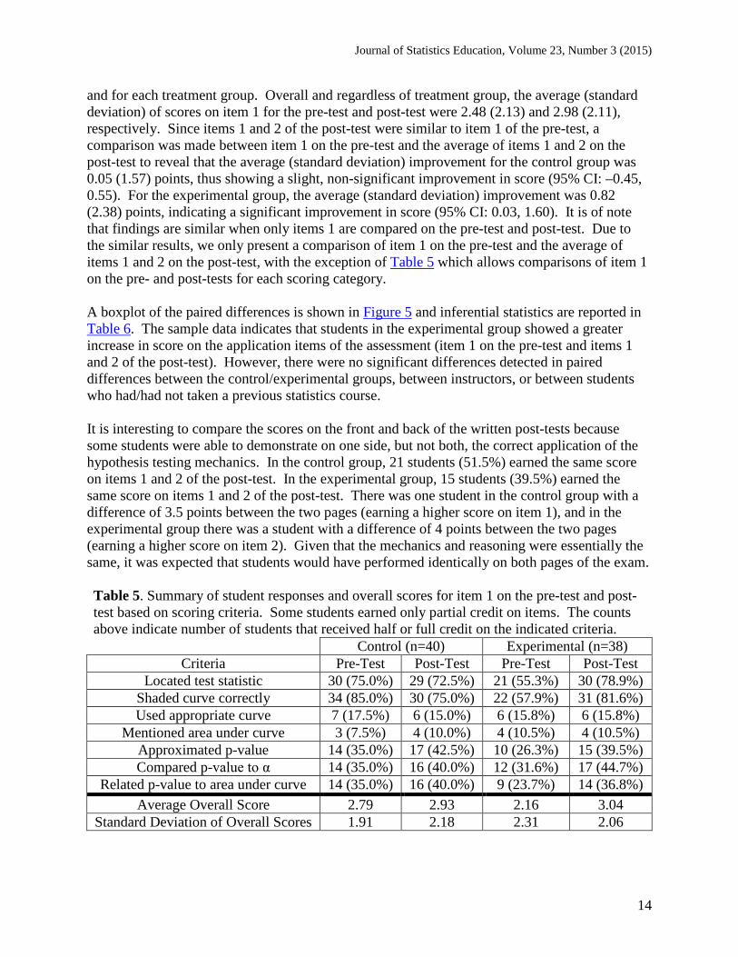
As part of the pre- and post-tests, students were also asked to complete a select-all-that-apply question in order to assess several issues noted by the instructors (item 5 on the pre-test and item 6 on the post-test). This item prompted students to select all of the statements which were true when a sampling distribution is unknown. In particular, the instructors were interested in tracking the number of students who did not understand that the sampling distribution is theoretically dictated based on the data and test chosen. In other words, the instructors were interested in tracking the number of students who viewed the t-distribution (or normal distribution) as a default sampling distribution to use for generating p-values. 6. Analysis of Pre- and Post-Test Responses Frequencies of student responses in the evaluative categories from Section 5 and summaries of overall scores on item 1 from the pre-test and post-test are tabulated in Table 5. The counts reported in the table represent the number of students who received at least half credit on each of the 7 criteria used for computing their total score. Counts have been reported for each criterion


14

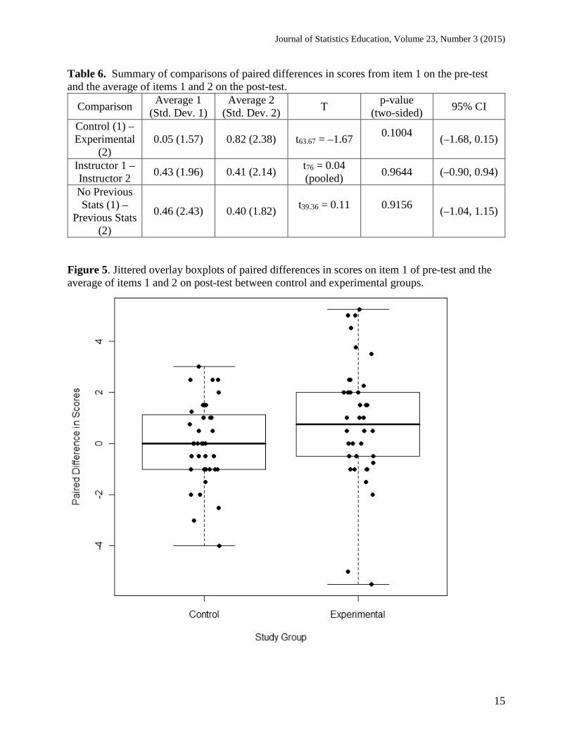
and for each treatment group. Overall and regardless of treatment group, the average (standard deviation) of scores on item 1 for the pre-test and post-test were 2.48 (2.13) and 2.98 (2.11), respectively. Since items 1 and 2 of the post-test were similar to item 1 of the pre-test, a comparison was made between item 1 on the pre-test and the average of items 1 and 2 on the post-test to reveal that the average (standard deviation) improvement for the control group was 0.05 (1.57) points, thus showing a slight, non-significant improvement in score (95% CI: –0.45, 0.55). For the experimental group, the average (standard deviation) improvement was 0.82 (2.38) points, indicating a significant improvement in score (95% CI: 0.03, 1.60). It is of note that findings are similar when only items 1 are compared on the pre-test and post-test. Due to the similar results, we only present a comparison of item 1 on the pre-test and the average of items 1 and 2 on the post-test, with the exception of Table 5 which allows comparisons of item 1 on the pre- and post-tests for each scoring category. A boxplot of the paired differences is shown in Figure 5 and inferential statistics are reported in Table 6. The sample data indicates that students in the experimental group showed a greater increase in score on the application items of the assessment (item 1 on the pre-test and items 1 and 2 of the post-test). However, there were no significant differences detected in paired differences between the control/experimental groups, between instructors, or between students who had/had not taken a previous statistics course. It is interesting to compare the scores on the front and back of the written post-tests because some students were able to demonstrate on one side, but not both, the correct application of the hypothesis testing mechanics. In the control group, 21 students (51.5%) earned the same score on items 1 and 2 of the post-test. In the experimental group, 15 students (39.5%) earned the same score on items 1 and 2 of the post-test. There was one student in the control group with a difference of 3.5 points between the two pages (earning a higher score on item 1), and in the experimental group there was a student with a difference of 4 points between the two pages (earning a higher score on item 2). Given that the mechanics and reasoning were essentially the same, it was expected that students would have performed identically on both pages of the exam. Table 5. Summary of student responses and overall scores for item 1 on the pre-test and post-test based on scoring criteria. Some students earned only partial credit on items. The counts above indicate number of students that received half or full credit on the indicated criteria.

Control (n=40) Experimental (n=38) Criteria Pre-Test Post-Test Pre-Test Post-Test

Located test statistic 30 (75.0%) 29 (72.5%) 21 (55.3%) 30 (78.9%) Shaded curve correctly 34 (85.0%) 30 (75.0%) 22 (57.9%) 31 (81.6%) Used appropriate curve 7 (17.5%) 6 (15.0%) 6 (15.8%) 6 (15.8%)

Mentioned area under curve 3 (7.5%) 4 (10.0%) 4 (10.5%) 4 (10.5%) Approximated p-value 14 (35.0%) 17 (42.5%) 10 (26.3%) 15 (39.5%) Compared p-value to α 14 (35.0%) 16 (40.0%) 12 (31.6%) 17 (44.7%)

Related p-value to area under curve 14 (35.0%) 16 (40.0%) 9 (23.7%) 14 (36.8%) Average Overall Score 2.79 2.93 2.16 3.04

Standard Deviation of Overall Scores 1.91 2.18 2.31 2.06


15

Table 6. Summary of comparisons of paired differences in scores from item 1 on the pre-test and the average of items 1 and 2 on the post-test.

Comparison Average 1 (Std. Dev. 1)

Average 2 (Std. Dev. 2) T p-value

(two-sided) 95% CI

Control (1) – Experimental

(2) 0.05 (1.57) 0.82 (2.38) t63.67 = –1.67 0.1004

(–1.68, 0.15)

Instructor 1 – Instructor 2 0.43 (1.96) 0.41 (2.14) t76 = 0.04

(pooled) 0.9644 (–0.90, 0.94)

No Previous Stats (1) –

Previous Stats (2)

0.46 (2.43) 0.40 (1.82) t39.36 = 0.11

0.9156 (–1.04, 1.15)

Figure 5. Jittered overlay boxplots of paired differences in scores on item 1 of pre-test and the average of items 1 and 2 on post-test between control and experimental groups.


16

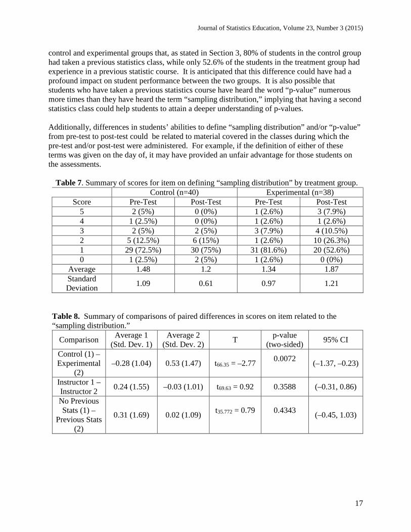
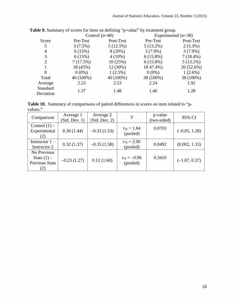
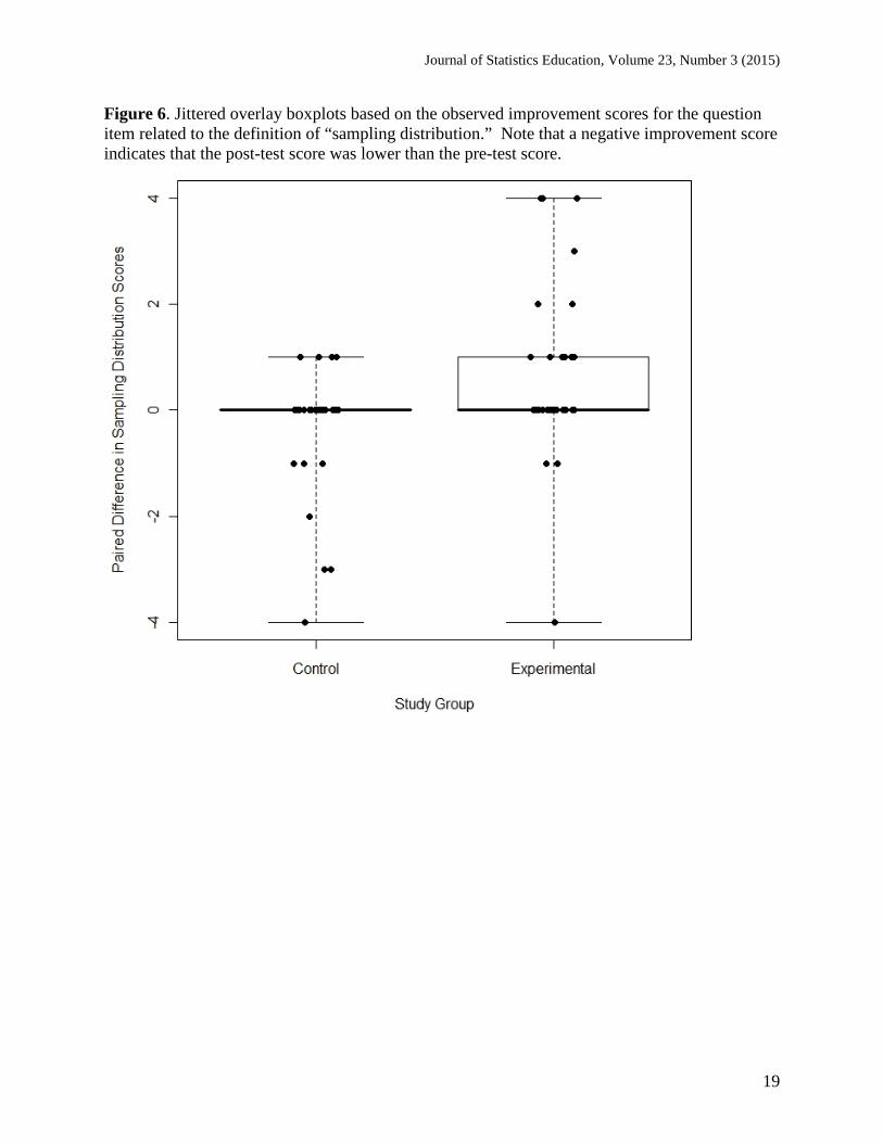
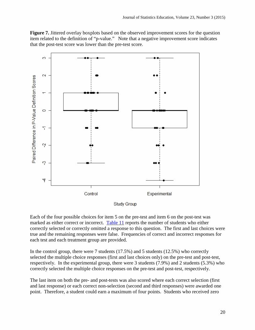
Responses to the items on “sampling distribution” and “p-value” were markedly more difficult to score. There were many instances where the authors had to balance what students implied with their choice of words and what was truly omitted from their responses. With the combined data from both treatment groups, the average (standard deviation) of scores on the “sampling distribution” definition were 1.41 (1.02) and 1.53 (1.00), respectively, on the pre-test and post-test. Table 7 and Table 9 tabulate student scores on the pre-test and post-test for defining the phrases “sampling distribution” and “p-value,” respectively, for each of the treatment groups. Pre-test and posts-test scores for the definition of “sampling distribution” items were paired based on student to reveal that the average (standard deviation) improvement for the control group was -0.28 (1.04) points, indicating a slight, non-significant decrease in score (95% CI: –0.61, 0.06). For the experimental group, the average (standard deviation) in change in score was 0.53 (1.47) points, implying a significant improvement in score (95% CI: 0.04, 1.01). This indicates that, on average, students in the control group became worse at interpreting a sampling distribution, while, on average, students in the experimental group improved their sampling distribution definition. A boxplot of the paired differences is shown in Figure 6, and inferential statistics are reported in Table 8. There was convincing evidence of a higher improvement in scores for the experimental group on the “sampling distribution” item of the pre-test and post-test than for the control group. Again, there was no evidence of an instructor effect or a previous statistics course effect on the paired differences in the scores for the “sampling distribution” definition question. Although the experimental group showed more improvement than the control group with the “sampling distribution” definition item, this was not true for the “p-value” definition item. The overall average (standard deviation) of the 78 student scores associated with the “p-value” definition were 2.23 (1.40) and 2.23 (1.41), respectively, on the pre-test and post-test. Pre-test and posts-test scores for the definition of “p-value” items were again paired based on student to reveal that the average (standard deviation) improvement for the control group was 0.30 (1.44) points. This indicates a slight, non-significant increase in score (95% CI: –0.16, 0.76). For the experimental group, the average (standard deviation) improvement was -0.32 (1.53) points. This shows a small, non-significant decrease in score (95% CI: –0.82, 0.19). Therefore, the sample data indicate that, on average, the control group improved in their “p-value” definition while, on average, the experimental group did worse on the post-test compared to the pre-test. Figure 7 shows a boxplot of the paired differences related to the “p-value” definition, and inferential statistics are reported in Table 10. There was some inconclusive evidence of positive improvement in scores for the control group over the experimental group on the paired differences in scores related to the “p-value” definition. Also, there was marginal evidence of an instructor effect on the paired differences in the scores for the “p-value” definition questions. There was no evidence of a difference in improvements based on whether or not a student had previously taken a statistics course. Therefore, on average, the experimental group decreased in their ability to define a p-value, while the control group, on average showed some improvement. This is a phenomenon that we did not expect to happen. However, it should be noted when making comparisons between the


17

control and experimental groups that, as stated in Section 3, 80% of students in the control group had taken a previous statistics class, while only 52.6% of the students in the treatment group had experience in a previous statistic course. It is anticipated that this difference could have had a profound impact on student performance between the two groups. It is also possible that students who have taken a previous statistics course have heard the word “p-value” numerous more times than they have heard the term “sampling distribution,” implying that having a second statistics class could help students to attain a deeper understanding of p-values. Additionally, differences in students’ abilities to define “sampling distribution” and/or “p-value” from pre-test to post-test could be related to material covered in the classes during which the pre-test and/or post-test were administered. For example, if the definition of either of these terms was given on the day of, it may have provided an unfair advantage for those students on the assessments.

Table 7. Summary of scores for item on defining “sampling distribution” by treatment group. Control (n=40) Experimental (n=38)

Score Pre-Test Post-Test Pre-Test Post-Test 5 2 (5%) 0 (0%) 1 (2.6%) 3 (7.9%) 4 1 (2.5%) 0 (0%) 1 (2.6%) 1 (2.6%) 3 2 (5%) 2 (5%) 3 (7.9%) 4 (10.5%) 2 5 (12.5%) 6 (15%) 1 (2.6%) 10 (26.3%) 1 29 (72.5%) 30 (75%) 31 (81.6%) 20 (52.6%) 0 1 (2.5%) 2 (5%) 1 (2.6%) 0 (0%)

Average 1.48 1.2 1.34 1.87 Standard Deviation 1.09 0.61 0.97 1.21

Table 8. Summary of comparisons of paired differences in scores on item related to the “sampling distribution.”



(two-sided) 95% CI


(2) –0.28 (1.04) 0.53 (1.47) t66.35 = –2.77 0.0072

(–1.37, –0.23)

Instructor 1 – Instructor 2 0.24 (1.55) –0.03 (1.01) t69.63 = 0.92 0.3588 (–0.31, 0.86)


Previous Stats (2)

0.31 (1.69) 0.02 (1.09) t35.772 = 0.79

0.4343 (–0.45, 1.03)


18

Table 9. Summary of scores for item on defining “p-value” by treatment group. Control (n=40) Experimental (n=38)

Score Pre-Test Post-Test Pre-Test Post-Test 5 3 (7.5%) 5 (12.5%) 5 (13.2%) 2 (5.3%) 4 6 (15%) 8 (20%) 3 (7.9%) 3 (7.9%) 3 6 (15%) 4 (10%) 6 (15.8%) 7 (18.4%) 2 7 (17.5%) 10 (25%) 6 (15.8%) 5 (13.2%) 1 18 (45%) 12 (30%) 18 47.4%) 20 (52.6%) 0 0 (0%) 1 (2.5%) 0 (0%) 1 (2.6%)

Total 40 (100%) 40 (100%) 38 (100%) 38 (100%) Average 2.23 2.53 2.24 1.92 Standard Deviation 1.37 1.48 1.46 1.28

Table 10. Summary of comparisons of paired differences in scores on item related to “p-values.”



(two-sided) 95% CI


(2) 0.30 (1.44) –0.32 (1.53) t76 = 1.84

(pooled) 0.0703

(–0.05, 1.28)

Instructor 1 – Instructor 2 0.32 (1.37) –0.35 (1.58) t76 = 2.00

(pooled) 0.0492 (0.002, 1.33)


Previous Stats (2)

–0.23 (1.27) 0.12 (1.60) t76 = –0.96 (pooled)

0.3410 (–1.07, 0.37)


19

Figure 6. Jittered overlay boxplots based on the observed improvement scores for the question item related to the definition of “sampling distribution.” Note that a negative improvement score indicates that the post-test score was lower than the pre-test score.


20

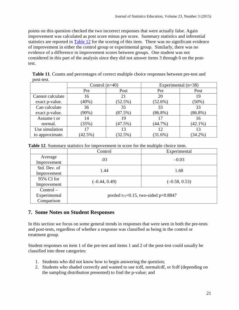
Figure 7. Jittered overlay boxplots based on the observed improvement scores for the question item related to the definition of “p-value.” Note that a negative improvement score indicates that the post-test score was lower than the pre-test score. Each of the four possible choices for item 5 on the pre-test and item 6 on the post-test was marked as either correct or incorrect. Table 11 reports the number of students who either correctly selected or correctly omitted a response to this question. The first and last choices were true and the remaining responses were false. Frequencies of correct and incorrect responses for each test and each treatment group are provided. In the control group, there were 7 students (17.5%) and 5 students (12.5%) who correctly selected the multiple choice responses (first and last choices only) on the pre-test and post-test, respectively. In the experimental group, there were 3 students (7.9%) and 2 students (5.3%) who correctly selected the multiple choice responses on the pre-test and post-test, respectively. The last item on both the pre- and post-tests was also scored where each correct selection (first and last response) or each correct non-selection (second and third responses) were awarded one point. Therefore, a student could earn a maximum of four points. Students who received zero


21

points on this question checked the two incorrect responses that were actually false. Again improvement was calculated as post score minus pre score. Summary statistics and inferential statistics are reported in Table 12 for the scoring of this item. There was no significant evidence of improvement in either the control group or experimental group. Similarly, there was no evidence of a difference in improvement scores between groups. One student was not considered in this part of the analysis since they did not answer items 3 through 6 on the post-test.

Table 11. Counts and percentages of correct multiple choice responses between pre-test and post-test.

Control (n=40) Experimental (n=38) Pre Post Pre Post

Cannot calculate exact p-value.

16 (40%)

21 (52.5%)

20 (52.6%)

19 (50%)

Can calculate exact p-value.

36 (90%)

35 (87.5%)

33 (86.8%)

33 (86.8%)

Assume t or normal.

14 (35%)

19 (47.5%)

17 (44.7%)

16 (42.1%)

Use simulation to approximate.

17 (42.5%)

13 (32.5%)

12 (31.6%)

13 (34.2%)

Table 12. Summary statistics for improvement in score for the multiple choice item.

Control Experimental Average

Improvement .03 –0.03

Std. Dev. of Improvement 1.44 1.68

95% CI for Improvement (–0.44, 0.49) (–0.58, 0.53)

Control – Experimental Comparison

pooled t75=0.15, two-sided p=0.8847

7. Some Notes on Student Responses In this section we focus on some general trends in responses that were seen in both the pre-tests and post-tests, regardless of whether a response was classified as being in the control or treatment group. Student responses on item 1 of the pre-test and items 1 and 2 of the post-test could usually be classified into three categories:

1. Students who did not know how to begin answering the question; 2. Students who shaded correctly and wanted to use tcdf, normalcdf, or fcdf (depending on

the sampling distribution presented) to find the p-value; and


22

3. Students who recognized the need to find the area they shaded on the sampling distribution provided.

In general a student would earn two points if they used the test statistic (either located it on the curve or used it in some cdf syntax) and shaded in the appropriate direction (either shaded on the curve or implied it based on provided cdf syntax). This was one of the most popular ways to earn two points. It is interesting to note that 52 students (66.7%) scored at least two points on item 1 of the pre-test and 55 students (70.5%) scored at least two points on item 1 of the post-test. Additionally, 61.5% of students located and shaded correctly on the pre-test for item 1, and 66.7% of students located and shaded correctly on the post-test for item 1. Table 5 clearly indicates the strength that students have for correctly locating the test statistic and shading in the appropriate direction. These are fairly formulaic skills. It is encouraging that many students located the test statistic (and not the null value) on the sampling distribution, even in the scenario where students shaded the picture properly but could not explain how to calculate the p-value from the picture. However, less than half of the students in both groups could accurately approximate the p-value, even on the post-test. This suggests that it may be important for instructors to build on the idea of why we locate values of test statistics on sampling distributions when reinforcing the concept of sampling distributions. The lower scores shown in Table 5 also indicate that students struggle with the broader conceptualization of what is happening when they are calculating a p-value and what the p-value can then ultimately tell them. Another positive result observed was that students understand the mechanics of how to use the hypotheses in order to determine the appropriate shading on the sampling distribution. Also, it was promising that many students were trying to match up the distribution to one they knew of as opposed to earlier worries by the instructors that students thought we used the t-distribution (specifically, tcdf on the TI-84 calculator) to calculate all p-values for all curves. However, there were still a fairly large number of student responses that were similar to “I would use tcdf to calculate the p-value” or would provide code that involved tcdf to demonstrate how they would use the information provided to calculate a p-value even when the curve was clearly not a t-distribution. This suggests a strong inclination toward using technology to answer everything and a lack of understanding of how to apply and synthesize hypothesis testing concepts. As a reminder, in part (c) of item 1 on the pre-test and in part (c) of items 1 and 2 of the post-test, students could earn a maximum of two points. To earn both points, the student had to indicate that they were looking at the area that was shaded in part (a) of the question, and indicate that they made a comparison to the significance level. In our data, 73.1% of students earned no credit on part (c) of item 1 on the pre-test, and 62.8% of students earned no credit on part (c) of item 1 on the post-test. Almost no students mentioned the word “area” in their responses on how to find the p-value, though most of the time they had a general notion or implied that we were looking for the shaded region of the graph. Many students lacked precision in providing explanations for their reasoning. Ideally, students would have responded similarly to the student response in Figure 2. Typical statements often


23

referenced the size of the shaded portion of the curve, but not necessarily with a comparison to the value of 5%. Some of the most concerning responses were those where students, regardless of how unsuccessful they were at being able to demonstrate how to calculate the p-value, were able to select an answer regarding the size of the p-value and ultimately provide justification for their selection that used inappropriate reasoning, such as:

• Saying that a majority of the curve is larger/smaller than the null value; • Comparing the test statistic to the null value and discussing the likelihood of this

difference; • Comparing the test statistic to a value that was not provided, such as the mean; or • Making decisions about the size of the p-value based on whether or not there was a lot of

evidence for the mean given. (It was unclear how they knew this without having the p-value.)

For item 1 on the pre-test and items 1 and 2 on the post-test, some anomalies in student responses should be mentioned.

• Some students discussed log transforming the data (which was actually the sampling distribution). This is attributed to covering a section on log transformations prior to covering ANOVA in the class.

• Several students tried to use a classical approach with the test statistic representing the critical value and determining if the null value falls in the shaded region. This is also attributed to covering a section on the classical approach prior to covering ANOVA.

• Students sometimes stated that they knew they would get a small p-value (or vice versa) because the alternative was true (or vice versa) when they had no information that would indicate to them that the alternative was true in the absence of a p-value or location of test statistic on the sampling distribution.

In the survey item related to the definition of “sampling distribution,” there were several themes in student responses. Students mistakenly thought that the sampling distribution was the distribution of a sample or the spread or range of our sample. To illustrate, one student responded, “The sampling distribution describes Shape, Center, and Spread of the data that you are analyzing.” Other students were very unsuccessful at defining “sampling distribution.” For example, one student responded “A sampling distribution is the number of objects/individuals/test subjects that are taken from a greater population in order to make assumptions about the greater population.”

We now return our attention to the survey item on both the pre- and post-tests which asked about the definition of a “p-value.” In the advanced introductory course in which we carried out our new randomization-based activity, students are taught the standard definition of a p-value as: the probability of observing our test statistic or something more extreme if the null hypothesis was true. Students generally earned a score of “4=mostly accurate response” for the “p-value” definition items when they omitted one portion of the standard definition, such as “or more extreme” or “if the null was true.” For the post-test, one student omitted the word “probability”


24

but had all other components correct. Many students omitted an actual definition of p-value and instead talked about how to make a decision based on the size of the p-value. These students earned two points toward the definition out of five. This indicates that students are just following procedures (such as “Reject the H0 when the p is low”), and they do not have a strong conceptual understanding of the process. On both tests it was noted that a lot of students attempted to define “p-value” as the probability that the null hypothesis was true. A few students even reported that a p-value was the probability that the alternative hypothesis is true. Others just reported that it was the probability of the hypothesis being true (without specifying a hypothesis). Out of 78 overall pre-test responses, 24 students (30.8%) reported some variation of the null hypothesis or a hypothesis is true. On the pre-test there were also 4 students (5.1%) who indicated the definition of a p-value was the probability of the alternative hypothesis being true. Of the 76 completed responses on the post-test for this item, 22 students (29.0%) indicated a p-value was the probability of the null hypothesis being true and 3 students (4.0%) reported that a p-value was the probability of the alternative hypothesis being true.

8. Conclusion 8.1 Instructor’s Notes/Tips

In order to enhance the activity, the authors have had success engaging students through the use of multiple technologies. For example, students record the value of their test statistics using a Google Form prepared by the instructor. Taylor and Doehler (2014) provide additional information on the use of Google Forms for teaching purposes. In classrooms where instructors have access to the internet and projection screens, student responses submitted through the Google Form can be projected during class. This gives students an idea about the test statistics that other students are obtaining in the randomization activity. In particular, students begin to notice that all of the values of the test statistic are positive, and that the sampling distribution is skewed right, which are both important characteristics for students to be aware of when transitioning from normal and t-distributions to the F-distribution. Students are also able to visually observe the simulated sampling distribution for the maximum value which provides insight into the unusualness of the test statistic for the observed data. When using student randomized data in class, there is often not enough time in one class for students to perform enough randomizations in order to see the pattern in the sampling distribution clearly. There are two useful solutions to this based on how often these activities are performed. For an initial use of the application, an instructor is encouraged to use a computer program, such as R, to generate the appropriate calculations for several 100 or 1000 randomizations. These simulated values can be pre-loaded into the Google Form spreadsheet where student responses are collected so that they are seamlessly included in any graphics later developed. For instructors who repeatedly use an activity, it is helpful to have students use the same Google Form for submitting responses each semester in order to build up a stockpile of calculations. The drawbacks to this method are that there are often errors in the values reported, and it would be necessary to make these corrections to the historical data set so that incorrect responses are not forever perpetuated.


25

For classes that are held in a computer lab, students can be further engaged in computer software if the instructor shares the simulated F-statistic values via e-mail or a course web page. This allows students to work with and graphically display the simulated sampling distribution. Also, students’ use of statistical technology can be reinforced by having students explore descriptive statistics in order to better understand the connection between an unusual test statistic and the size of the p-value. Another option besides having students use an Excel spreadsheet to generate the F-test statistic is to have students compute the F-test statistic on their own. However, this is rather tedious and time consuming, and can not only distract from the flow of the activity, but also result in F-test statistics which are incorrect due to computational errors. Additionally, after the randomization activity and discussion have concluded, we use class time to go through the steps of computing an F-test statistic by hand using the original cereal data. However, using the Excel calculator which generates the F-test statistic for students can add to the mystery of ANOVA. To address this issue, a reviewer on a previous version of this manuscript suggested that students could begin by using a statistic which can easily be calculated by them, such as the mean of the absolute pairwise differences in group means. Once the groundwork of the process has been set using randomization-based methods, students can then be introduced to the F-test statistic and to the formal process of ANOVA. Another useful aspect of this data is the fact that one of the stores caught fire during the study, which is an interesting characteristic that allows for student buy-in on the real nature of the data. Students can also be asked about their majors to further engage them in the analysis by relating how different majors, such as business and marketing, might be involved in a similar study. Additionally, there are several ways in which the activity and its implementation can be improved. The use of the word “curve” should be avoided when referring to the simulated sampling distribution as the word “curve” implies continuity, which will not occur with simulated sampling distributions. For students, the connections between the simulated sampling distribution and the F distribution need to be made explicit. To aid in this, it is helpful to have used randomization-based methods previously in class. We refer the reader to a collection of randomization-based methods from Rossman and Chance (2008). Similarly, the transition between the “proportion of simulated statistics” and “area” is a jump of equal concern for students to make, and these connections must be made explicit for students. To aid in this, it is useful to orient the students’ perspectives as calculating the proportion of simulated statistics that are less/greater than or equal to an observed statistic when using randomization-based approaches and prior to making the transition to the use of the word “area” in the context of the F distribution. Lock Morgan, Lock, and Lock (2015) presented on the topic of “Connecting simulation-based inference with traditional methods,” and suggested that there are three transitions for students to make between simulation-based methods and theoretical methods: distribution, statistic, and standard error. They provide several techniques for accomplishing the goal of making connections.


26

8.2 Limitations and Future Research In analyzing the responses to the item which asked students to “Demonstrate how you would use this information to compute a p-value,” we noticed that students wanted to calculate a p-value answer and shied away from explaining how they would calculate it. For future use of the assessment items developed, the word “demonstrate” should be changed to “explain,” since students thought giving calculator code was demonstrating how to do it (though they were demonstrating it incorrectly). Additionally, students should be prompted to answer the questions without using their calculator to avoid students using brute force methods to obtain a p-value of any kind. This limited students’ abilities when asked to explain how they determined if the p-value would be less than 0.05 or greater than 0.05 since they only referred to their calculation and ignored the pictures that they had drawn. In essence, students almost completely by-passed using the sampling distribution provided. For future studies (and even future activities that are carried out in the classroom), instructors may want to refer to the sampling distribution as the “re-sampling” distribution. The phrase “sampling distribution” appears to be inherently dangerous. In other words, students mistake the word “sampling” to be synonymous with “sample,” and therefore view “sampling distributions” as the distribution of a sample. Additionally, in the pre- and post-tests, many students stated that they knew they would get a small p-value (or vice versa) because the alternative was true (or vice versa) without making connections between the sampling distribution, test statistic, and hypotheses that were provided. In the future, it would be interesting to further explore the thought patterns of these students to determine how they are coming to their conclusions in order to remedy this faulty non-evidenced based decision making. There are limitations of the study conducted that should be mentioned, along with recommendations for future similar studies. Limitations of this research include assessing student responses for only one semester and not using the exact same amount of class time to introduce ANOVA in both the treatment and control sections. It is recommended that, if possible, future studies be carried out over multiple semesters. More studies over numerous semesters may also help to set up the experiment in such a way that there are approximately equal percentages of students in both the treatment and control groups who have taken a previous statistics course. Additionally, we also advocate that in future research studies of this nature, the class time spent on specific topics is the same among both control and treatment groups. It is worth emphasizing that the experiences in the control and treatment groups in the course were similar if not identical with the exception of the randomization-based ANOVA activity. The actual instruction relevant to ANOVA was largely the same between the two groups and instructors. Students in both groups had a very similar background in the course leading up to this lesson. This common background could have had a strong impact on the limited number of significant differences detected in this study since students in the control and treatment groups had prior experience in the course with inferential statistics and randomization-based methods. One thing that makes our randomization activity different from many other randomization activities is that students never actually carry out a computer simulation. Instead we rely on students randomly generating the permuted data sets by hand. Although assessment of this study


27

was only carried out in one semester, we have been using the randomization activity itself for numerous semesters. We are able to utilize F-test statistics that were generated in previous semesters as well, so that when a graph of the sampling distribution is generated, it does not have to include only the test statistics that were generated in that class. For future research projects, it would be interesting to compare student understanding of sampling distributions between courses which rely on computer simulations, courses which utilize hands-on simulations, and hybrid courses which utilize both types of simulations. Undoubtedly, a major drawback of exclusively using hands-on simulations in a class is the large amount of class time that is required. However, in the event that students obtain and retain deep understanding of challenging statistical concepts through this time-consuming approach, it may be worth it. The randomization-based activity discussed in this paper promotes an intuitive approach to understanding concepts such as the definition of sampling distribution, while simultaneously introducing the challenging topic of ANOVA. The activity serves to demystify the origins of the sampling distribution and its importance in hypothesis testing. Our study reiterates the difficulty students have in understanding these important topics in statistical inference, and shows that gains in student understanding of sampling distributions are possible with the activity that was implemented. Additionally, while carrying out this and other randomization-based activities in class, we have noticed that students seemed to enjoy the process of permuting the data themselves, and overall the class seemed very engaged in the activity and the analysis. While we did not employ any research related to student attitudes towards statistics, especially in courses using randomization-based methods, it would be an interesting avenue for future research as evidence indicates academic gains are correlated with student attitudes toward statistics (Emmioğlu and Capa-Aydin 2012). We agree with Rossman and Chance (2014) when they say that previous research studies allude to the idea that a randomization-based approach to teaching statistics is practical. Anecdotally, we see a lot of value in utilizing randomization-based activities to improve student understanding of inference. However, we are reminded of Webster West’s statement in his talk at the 2015 United States Conference on Teaching Statistics that “Resampling is not a magic bullet by any means” (West 2015). Although our activity has shown promise in increasing understanding of sampling distributions, our study did not indicate that the experimental group improved significantly more in their understanding of inference compared to the control group. We recommended that researchers continue to investigate possible differences in student learning between randomization-based, non-randomization-based, and hybrid statistics curriculum.


28

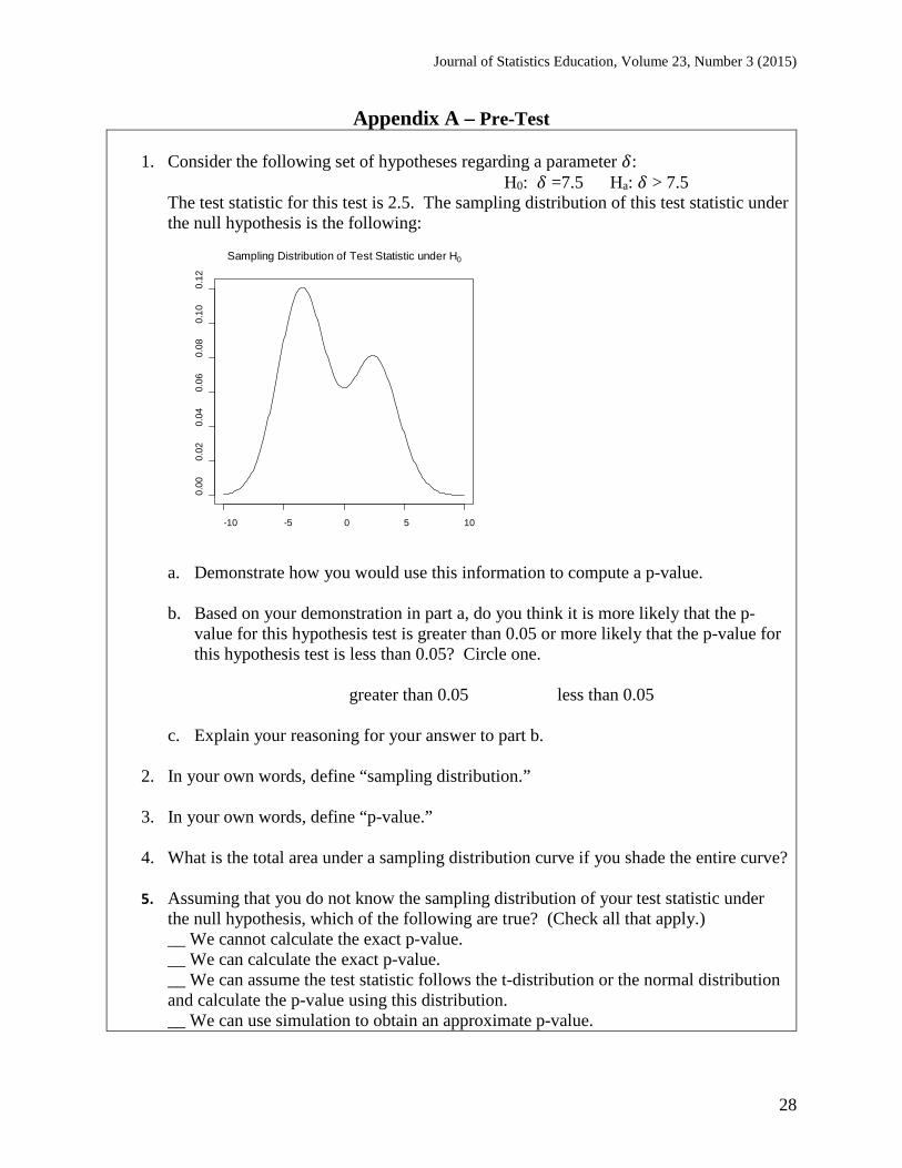
Appendix A – Pre-Test

1. Consider the following set of hypotheses regarding a parameter 𝛿𝛿: H0: 𝛿𝛿 =7.5 Ha: 𝛿𝛿 > 7.5 The test statistic for this test is 2.5. The sampling distribution of this test statistic under the null hypothesis is the following:

a. Demonstrate how you would use this information to compute a p-value.

b. Based on your demonstration in part a, do you think it is more likely that the p-

value for this hypothesis test is greater than 0.05 or more likely that the p-value for this hypothesis test is less than 0.05? Circle one. greater than 0.05 less than 0.05

c. Explain your reasoning for your answer to part b.

2. In your own words, define “sampling distribution.”

3. In your own words, define “p-value.”

4. What is the total area under a sampling distribution curve if you shade the entire curve?

5. Assuming that you do not know the sampling distribution of your test statistic under the null hypothesis, which of the following are true? (Check all that apply.) __ We cannot calculate the exact p-value. __ We can calculate the exact p-value. __ We can assume the test statistic follows the t-distribution or the normal distribution and calculate the p-value using this distribution. __ We can use simulation to obtain an approximate p-value.

-10 -5 0 5 10

0.00

0.02

0.04

0.06

0.08

0.10

0.12

Sampling Distribution of Test Statistic under H0


29

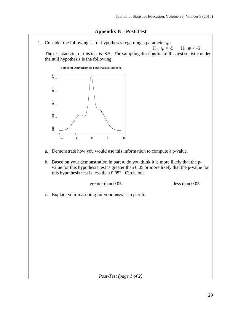
Appendix B – Post-Test

1. Consider the following set of hypotheses regarding a parameter 𝜓𝜓: H0: 𝜓𝜓 = -5 Ha: 𝜓𝜓 < -5 The test statistic for this test is -8.5. The sampling distribution of this test statistic under the null hypothesis is the following:





Post-Test (page 1 of 2)

-10 -5 0 5 10

0.00

0.05

0.10

0.15

0.20



30

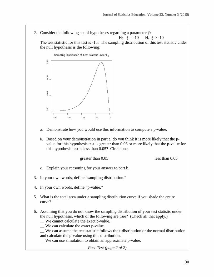
2. Consider the following set of hypotheses regarding a parameter 𝜉𝜉:

H0: 𝜉𝜉 = -10 Ha: 𝜉𝜉 > -10 The test statistic for this test is -15. The sampling distribution of this test statistic under the null hypothesis is the following:





3. In your own words, define “sampling distribution.”

4. In your own words, define “p-value.”

5. What is the total area under a sampling distribution curve if you shade the entire curve?

6. Assuming that you do not know the sampling distribution of your test statistic under the null hypothesis, which of the following are true? (Check all that apply.) __ We cannot calculate the exact p-value. __ We can calculate the exact p-value. __ We can assume the test statistic follows the t-distribution or the normal distribution and calculate the p-value using this distribution. __ We can use simulation to obtain an approximate p-value.

Post-Test (page 2 of 2)

-20 -15 -10 -5 0

0.00

0.05

0.10

0.15



31

Acknowledgements The first author would like to thank Elon University for a course reassignment provided to aid in this research. Both authors thank the reviewers and editor of this manuscript for providing significant improvements to the clarity and narrative of this paper. References Aliaga, M., Cobb, G., Cuff, C., Garfield, J., Gould, R., Lock, R., Moore, T., Rossman, A., Stephenson, B., Utts, J., Velleman, P., and Witmer, J. (2005), “Guidelines for Assessment and Instruction in Statistics Education (GAISE): College Report,” USA: American Statistical Association. Braun, W. (2012), “Naïve Analysis of Variance,” Journal of Statistics Education, 20(2), http://www.amstat.org/publications/jse/v20n2/braun.pdf Cobb, G. W. (2007), “The Introductory Statistics Course: A Ptolemaic Curriculum?,” Technology Innovations in Statistics Education, 1(1). Retrieved from: http://escholarship.org/uc/item/6hb3k0nz Emmioğlu, E., and Capa-Aydin, Y. (2012), “Attitudes and Achievement In Statistics: A Meta-Analysis Study,” Statistics Education Research Journal, 11(2). http://iase-web.org/documents/SERJ/SERJ11(2)_Emmioglu.pdf delMas, R., Garfield, J., and Chance, B. L. (1999), “A Model of Classroom Research in Action: Developing Simulation Activities to Improve Students’ Statistical Reasoning,” Journal of Statistics Education, 7(3). www.amstat.org/publications/jse/secure/v7n3/delmas.cfm Duffy, S. (2010), “Random Numbers Demonstrate the Frequency of Type I Errors: Three Spreadsheets for Class Instruction,” Journal of Statistics Education, 18(2), http://www.amstat.org/publications/jse/v18n2/duffy.pdf Fisher, R.A. (1936), “The coefficient of racial likeness and the future of craniometry,” Journal of the Royal Anthropological Institute of Great Britain and Ireland, 66, 57-63. Kutner, M., Nachtsheim, C., Neter, J., and Li, W. (2005), Applied Linear Statistical Models, 5th edition, 685-686, McGraw-Hill Irwin Lesser, L., and Melgoza, L. (2007), “Simple Numbers: ANOVA Example of Facilitating Student Learning in Statistics,” Teaching Statistics, 29(3), 102-105, doi: 10.1111/j.1467-9639.2007.00272.x Lock Morgan, K., Lock, P., and Lock, R. (2015), “Connecting simulation-based inference with traditional methods.” United States Conference on Teaching Statistics, State College, PA. May 29, 2015. Available at: http://www.personal.psu.edu/klm47/presentations.htm

http://www.amstat.org/publications/jse/v20n2/braun.pdf

http://escholarship.org/uc/item/6hb3k0nz

http://iase-web.org/documents/SERJ/SERJ11(2)_Emmioglu.pdf

http://iase-web.org/documents/SERJ/SERJ11(2)_Emmioglu.pdf

http://www.amstat.org/publications/jse/secure/v7n3/delmas.cfm

http://www.amstat.org/publications/jse/v18n2/duffy.pdf

http://www.personal.psu.edu/klm47/presentations.htm


32

Malloy, T. (2000), “Understanding ANOVA Visually.” Online statistical applet available at: http://web.utah.edu/stat/introstats/anovaflash.html Pfannkuch, M. (2007), “Year 11 students’ informal inferential reasoning: A case study about the interpretation of box plots,” International Electric Journal of Mathematics Education, 2(3), 149-167. Rossman, A. J., and Chance, B. L. (2000), “Teaching the reasoning of statistical inference: A ‘Top Ten’ List,” The Mathematical Association of America. Available online at: http://www.rossmanchance.com/papers/topten.html Rossman, A. J. (2008), “Reasoning about informal statistical inference: A statistician’s view,” Statistics Education Research Journal, 7(2), 5-19, https://www.stat.auckland.ac.nz/~iase/serj/SERJ7%282%29_Rossman.pdf Rossman, A. J. and Chance, B. L. (2008), “Concepts of Statistical Inference: A randomization-based curriculum,” Available at: http://statweb.calpoly.edu/csi Rossman A. J., and Chance B. L. (2014), “Using simulation‐based inference for learning introductory statistics,” WIREs Computational Statistics, 6(4), 211-221. Sturm-Beiss, R. (2005), “A Visualization Tool for One- and Two-Way Analysis of Variance,” Journal of Statistics Education [Online], 13(1), http://www.amstat.org/publications/jse/v13n1/sturm-beiss.html Taylor, L. and Doehler, K. (2014), “Using Online Surveys to Promote and Assess Learning”, Teaching Statistics, 36(2), 34-40, doi: 10.1111/test.12045/abstract Tintle, N., VanderStoep, J., Holmes, V.-L., Quisenberry, B., Swanson, T. (2011), “Development and assessment of a preliminary randomization-based introductory statistics curriculum,” Journal of Statistics Education [Online], 19(1), http://www.amstat.org/publications/jse/v19n1/tintle.pdf West, W. (2015), “What’s Wrong with ST101?,” United States Conference on Teaching Statistics, State College, PA. May 28, 2015. Available at: https://www.causeweb.org/uscots/uscots15/presentations/WebsterOpening.pdf Wild, C. J., Pfannkuch, M., Regan, M., and Horton, N. J. (2011), “Towards more accessible conceptions of statistic inference,” Journal of the Royal Statistical Society Series A, 174(2), doi: 10.1111/j.1467-985X.2010.00678.x

http://web.utah.edu/stat/introstats/anovaflash.html

http://www.rossmanchance.com/papers/topten.html

https://www.stat.auckland.ac.nz/%7Eiase/serj/SERJ7%282%29_Rossman.pdf

http://statweb.calpoly.edu/csi

http://www.amstat.org/publications/jse/v13n1/sturm-beiss.html

http://www.amstat.org/publications/jse/v19n1/tintle.pdf

https://www.causeweb.org/uscots/uscots15/presentations/WebsterOpening.pdf


33

Laura Taylor Department of Mathematics and Statistics Elon University Campus Box 2320 Elon, NC 27244 Email: [email protected] Phone: 336–278–6493 Kirsten Doehler Department of Mathematics and Statistics Elon University Campus Box 2320 Elon, NC 27244 Email: [email protected] Phone: 336–278–6473

Volume 23 (2015) | Archive | Index | Data Archive | Resources | Editorial Board | Guidelines for Authors | Guidelines for Data Contributors | Guidelines for Readers/Data Users | Home Page |

Contact JSE | ASA Publications

mailto:[email protected]


http://www.amstat.org/publications/jse/contents_2015.htm

http://www.amstat.org/publications/jse/jse_archive.htm

http://www.amstat.org/publications/jse/jse_index.htm

http://www.amstat.org/publications/jse/jse_data_archive.htm

http://www.amstat.org/publications/jse/jse_info_service.htm

http://www.amstat.org/publications/jse/jse_board.htm

http://www.amstat.org/publications/jse/jse_author_info.htm

http://www.amstat.org/publications/jse/jse_author_info.htm

http://www.amstat.org/publications/jse/jse_data_contributor_info.htm

http://www.amstat.org/publications/jse/jse_users.htm

http://www.amstat.org/publications/jse/


http://www.amstat.org/publications/

Documents

Reinforcing Sampling Distributions through a … Sampling Distributions through a Randomization-Based Activity for Introducing ANOVA . ... Section 2 of this paper provides a literature