Relational Learning as Search in a Critical Regionjmlr.csail.mit.edu/papers/volume4/botta03a/botta03a.pdfJournal of Machine Learning Research 4 (2003) 431-463 Submitted 5/01; Published

Journal of Machine Learning Research 4 (2003) 431-463 Submitted 5/01; Published 8/03

Relational Learning as Search in a Critical Region

Marco Botta [email protected] Giordana ATTILIO @MFN.UNIPMN.ITDipartimento di InformaticaUniversita di Torino10149, Torino, Italy

Lorenza Saitta [email protected] di Informatica, Universita del Piemonte Orientale15100 Alessandria, Italy

Michele Sebag [email protected]

Equipe Inference et Apprentissage, Lab. de Recherche en InformatiqueUniversite Paris-Sud Orsay91405 Orsay Cedex, France

Editors: James Cussens and Alan M. Frisch

AbstractMachine learning strongly relies on the covering test to assess whether a candidate hypothesis cov-ers training examples. The present paper investigates learning relational concepts from examples,termedrelational learningor inductive logic programming. In particular, it investigates the chancesof success and the computational cost of relational learning, which appears to be severely affectedby the presence of a phase transition in the covering test. To this aim, three up-to-date relationallearners have been applied to a wide range of artificial, fully relational learning problems. A firstexperimental observation is that the phase transition behaves as an attractor for relational learn-ing; no matter which region the learning problem belongs to, all three learners produce hypotheseslying within or close to the phase transition region. Second, afailure regionappears. All threelearners fail to learn any accurate hypothesis in this region. Quite surprisingly, the probability offailure does not systematically increase with the size of the underlying target concept: under somecircumstances, longer concepts may be easier to accurately approximate than shorter ones. Someinterpretations for these findings are proposed and discussed.

1. Introduction

In a seminal paper, Mitchell (1982) characterized machine learning (ML) as a search problem.Indeed, every learner basically explores some solution space until it finds a (nearly) optimal orsufficiently good solution. Since then much attention has been devoted to every component of asearch problem: the search space, the search goal, and the search engine.

The search space reflects the language chosen to express the target knowledge, called thehy-pothesis language. Although most works in ML consider attribute-value languages (Mitchell, 1982;Quinlan, 1986), first-order logic languages, or a subset thereof (Michalski, 1983), are required todeal with structured application domains such as chemistry or natural language processing. Thispaper focuses on learning in first-order logic languages, referred to asrelational learning(Quinlan,1990) orinductive logic programming(Muggleton and De Raedt, 1994). This task has been tack-

c©2003 Marco Botta, Attilio Giordana, Lorenza Saitta and Mich`ele Sebag.

BOTTA, GIORDANA, SAITTA AND SEBAG

led by many authors since the early 1990s, following Bergadano et al. (1991), Pazzani and Kibler(1992) and Muggleton and Feng (1992).

1.1 Relational Learning Complexity

In machine learning, assessing the quality of any hypothesis relies heavily on thecovering test,which verifies whether a given hypothesish is satisfied by an exampleE. In the logic-based approachto learning taken by inductive logic programming (ILP), the covering test most commonly used isθ-subsumption (Plotkin, 1970; Muggleton, 1992; Nienhuys-Cheng and de Wolf, 1997), which hasbeen proved to be an NP-hard problem (Nienhuys-Cheng and de Wolf, 1997). Then, a major con-cern facing relational learning is computational complexity. Most studies in computational learningare rooted in the PAC-learning framework proposed by Valiant (1984)1, and the literature offersmany results regarding the worst-case and average-case complexity of learning various classes ofrelational concepts (Cohen, 1993; D˘zeroski et al., 1992; Kietz and Morik, 1994; Khardon, 1998).

However, another emerging framework offers a more detailed perspective on complexity thanjust worst- and average-case analysis. This framework, initially developed in relation to searchproblems, is referred to as thephase transition (PT) framework(Hogg et al., 1996a), and it consid-ers computational complexity as a random variable that depends on someorder parametersof theproblem class at hand. Computational complexity is thus modeled as a distribution over probleminstances (statistical complexity).

The advantage of the statistical complexity paradigm is twofold. First, it accounts for the factthat, despite the exponential worst-case complexity of an NP-hard class of problems, most probleminstances are actually easy to solve; second, it shows that many very hard problem instances con-centrate in a narrow region, termed themushyregion (Hogg et al., 1996a). Most problem instances,in fact, are either under-constrained (they admit many solutions, and finding one of them is easy), orover-constrained (to such an extent that it is easy to show that no solution exists). Thus, the compu-tational complexity landscape of a problem class appears to be divided into three regions: the “YES”region, including the under-constrained problem instances, where the probability of any of them be-ing solvable is close to one; the “NO” region, including the over-constrained problem instances,where the probability of any of them being solvable is close to zero; and the narrow mushy region inbetween, across which the probability of a random problem instance being solvable abruptly dropsfrom almost one to almost zero. The mushy region includes the phase transition, defined as thelocus, in the parameter space, where the probability for a random problem instance being solvableis 0.5. Interestingly enough, it has been observed that a large peak in computational complexityusually appears in correspondence to the phase transition (Cheeseman et al., 1991; Williams andHogg, 1994; Hogg et al., 1996b; Walsh, 1998).2

To sum up, the phase transition region is, on average, the hardest part of the parameter space.This fact has many theoretical and practical implications. One such implication is that any complex-ity analysis should try to locate the PT region; to this aim, one must identify the order parameters forthe problem class at hand, and the critical values for these parameters corresponding to the locationof the phase transition. Second, any new algorithm must be evaluated on problem instances lyingin the PT region. Complexity results obtained on problem instances belonging to the YES or NO

1. For a detailed presentation see Kearns and Vazirani (1994).2. In this paper we will use the terms “mushy region” and “PT region” as synonyms.

432

LEARNING IN A CRITICAL REGION

regions are likely to be irrelevant for characterizing the class complexity, as pointed out by Hogget al. (1996a).

1.2 Phase Transition and Relational Learning

Previous experiments (Botta, Giordana, and Saitta, 1999; Botta, Giordana, Saitta, and Sebag, 2000;Giordana and Saitta, 2000) have shown the presence of a phase transition in the covering test, bothin artificial and real-world learning problems. Starting from the obtained results, this paper offersa deeper insight into the observed effects of the phase transition on the quality and complexityof learning. The initial focus in the work by Botta, Giordana, and Saitta (1999); Botta, Giordana,Saitta, and Sebag (2000) and by Giordana and Saitta (2000) was on complexity issues, especially onfinding ways around the dramatic complexity increase. However, this paper shows that the existenceof a phase transition in the covering test has much deeper and far reaching effects on the feasibilityof relational learning than just this increase in computational cost. Preliminary results in this newdirection have been presented by Giordana, Saitta, Sebag, and Botta (2000). The emergence of aphase transition impacts machine learning in at least three respects:

• A region of significant size around the phase transition appears to contain extremely difficultlearning problems.

• Popular search heuristics in machine learning, such asinformation gain(Quinlan, 1990) orminimum description length(Rissanen, 1978; Muggleton, 1995) are not reliable in the earlystages of top-down hypothesis generation. These heuristics, in fact, provide reliable informa-tion only when the search enters the phase transition region.

• A low generalization error of a learned hypothesis does not imply that the “true” target con-cept has been captured. This is particularly important for automated knowledge discovery,where a major issue is to provide experts with new relevant insights into the domain underanalysis. As a matter of fact, good approximations of a complex concept can only be foundnear the phase transition, irrespectively of the location of the concept. Then, discovering the“true” concept is extremely unlikely if it lies outside the phase transition region.

The above mentioned experiments have been performed using a problem generator originallydesigned to check the existence of a phase transition (Botta et al., 2000; Giordana and Saitta, 2000),and later extended to generate artificial, fully relational learning problemswith known target con-cept. A suite of some five hundred problems has been constructed, sampling the YES, NO and PTregions. A popular relational learner, FOIL 6.4 (Quinlan, 1990), has been systematically appliedto these problems. Moreover, two other learners, SMART+ (Botta and Giordana, 1993) and G-Net(Anglano et al., 1998), have been independently applied on a subset of the problems, selected inorder provide a comparison with different search strategies.

These systematic experiments shed some light on the behavior, capabilities and limitations ofexisting relational learners. First of all, for all three relational learners considered, the PT regionis actually an attractor in the sense that whatever the location of the learning problem, with respectto the phase transition, in most cases the learners conclude their search in the PT region. Second,a failure regionappears, where all three learners fail to discover either the target concept, or anyacceptable approximation thereof. The failure region largely overlaps the PT region; learning prob-lems close to the phase transition appear to be much harder than others. Unexpectedly, very long

433


concepts happen to be easier to learn than shorter ones under some circumstances. Interpretationsfor these findings are proposed, and their implications regarding relational learning are discussed.

The rest of the paper is organized as follows. To be self-contained, Section 2 summarizes pre-vious results regarding the existence and location of the phase transition for the covering test (thereader is referred to Giordana and Saitta, 2000, for a detailed presentation). Section 3 describesthe experimental setting used to estimate the impact of the phase transition on relational learning:learning problems sampling the three regions (under-constrained or YES-region, PT or mushy re-gion, over-constrained or NO-region) are constructed. Section 4 describes the empirical resultsobtained on these problems by FOIL (Quinlan, 1990), SMART+ (Botta and Giordana, 1993) andG-Net (Anglano et al., 1998). Some interpretations for these results are proposed in Section 5. Sec-tion 6 discusses the extent to which these findings lead to the reconsideration of the current biasesand search strategies for relational learning, and the paper ends with some suggestions for furtherresearch.

2. Phase Transition in Matching Problems

Machine learning proceeds by repeatedly generating and testing hypotheses; these hypotheses arerated according to (among other criteria) their coverage of training examples (Mitchell, 1997). Inthis paper, we will consider the simplest setting used in relational learning, where concepts aredescribed by sets of clauses in a restricted Datalog language (Date, 1995) having the form:

c : − h(X1,X2, . . . ,Xn). (1)

In (1) c is a classname3 andh a conjunction of literals that may contain variables or constants,but no function symbols; negation is allowed, but only on single literals on the right hand side.The variables occurring inh, if any, areX1,X2, . . . ,Xn As a matter of fact, Datalog is a hypothesislanguage largely used in relational learning (Muggleton and De Raedt, 1994; Nienhuys-Cheng andde Wolf, 1997), and concept descriptions in the form (1) have been used in many applications, sincethe early approach by Michalski (1983).

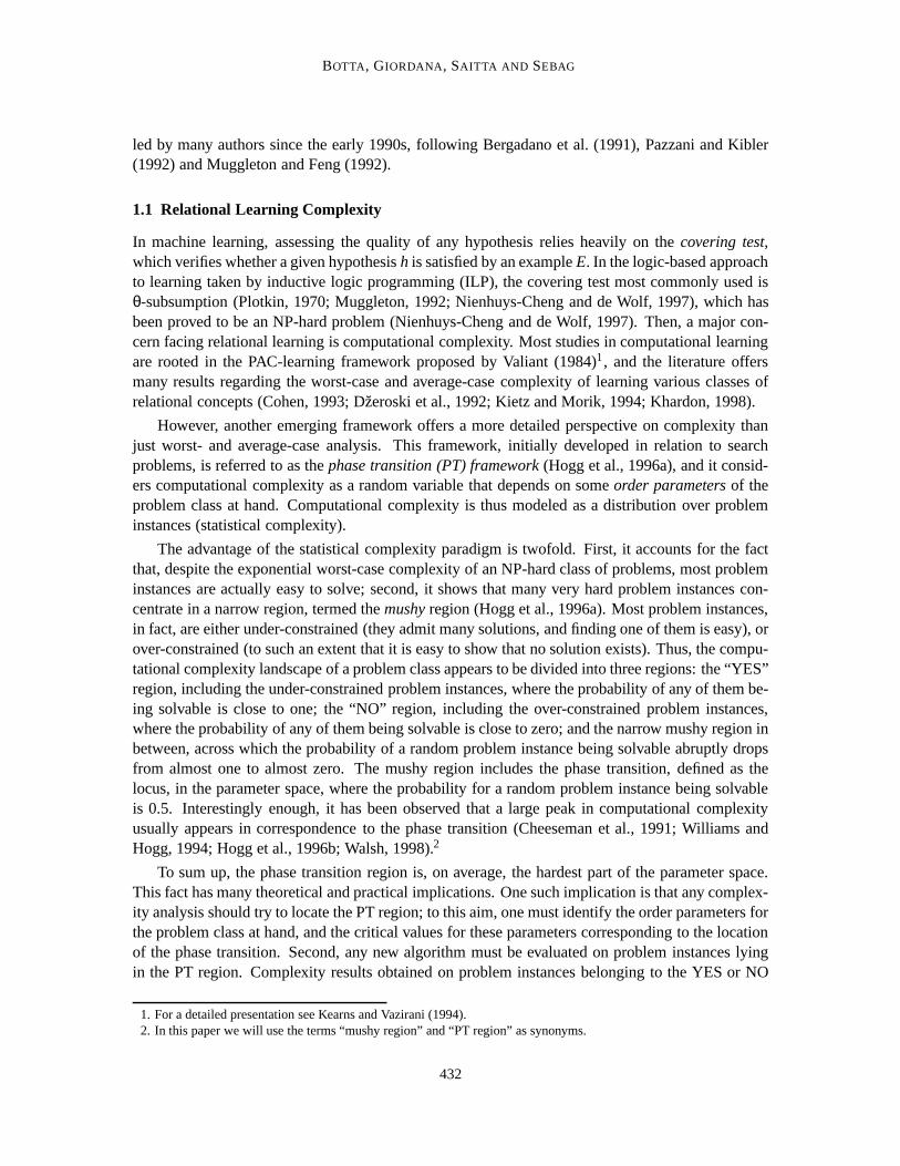
In several learning approaches, notably in data mining, an exampleE is described as a set oftables; each table corresponds to a basic predicater(X1,X2, . . . ,Xs) of the language, and each rowin the table is associated to a tuple of objects〈a1,a2, . . . ,as〉 in E such thatr(a1,a2, ...,as) is true.Figure 1 shows an example for the sake of illustration.

Alternatively, in the logical approach taken by ILP (Muggleton, 1992), examples are repre-sented as conjunctions of a possibly large number of ground facts (ground literals). The transfor-mation between tabular representation and ground literal representation is immediate: every row〈a1,a2, ...,as〉 in the table associated to a predicater is transformed into an equivalent ground literalr(a1,a2, ...,as). For instance, the exampleE in Figure 1 can be represented as follows:

E : on(a,b), on(c,d), le f t(a,c), le f t(a,d), le f t(b,c), le f t(b,d). (2)

All three learning algorithms used in this paper, namely FOIL (Quinlan, 1990), SMART+ (Bottaand Giordana, 1993) and G-Net (Anglano et al., 1998), use the tabular representation of the exam-ples, at least as the internal representation, and have been applied to the task of learning concepts inform (1).

3. We consider the simple case in which the head of the clause does not have variables.

434


bd

a

c

(a)

E X Y

a b

c d

on(X,Y)

X Y

a c

a d

left(X,Y)

b c

b d

(b)

X

a c

b c

left(X,Y),on(Y,Z)

d

d

Y Z

(c)

Figure 1: Tabular representation of structured examples of the block world. (a) Block world in-stanceE composed of four objects,a, b, c, andd. (b) Tables describingE, assuming thatthe description language contains only two predicates, namelyon(X,Y) and le f t(X,Y).(c) Two substitutions forX,Y,Z that satisfy the hypothesish = le f t(X,Y),on(Y,Z). Inparticular,h(a,c,d) = le f t(a,c),on(c,d) is true inE.

More precisely, given a description (an inductive hypothesis)h(X1,X2, . . . ,Xn) and an exampleE described by the finite setR = {r1, r2, ...., rm} of tables, letA be the set of all constants occurringin the tables ofR. Let us consider a substitutionθ = (X1/a1,X2/a2, ....Xn/an). Let ri(Xi1, ..,Xik) bea literal occurring inh and built on predicate symbolri . Let, moreover,(Xi1/ai1, ...,Xik/aik) be thesubstitution defined byθ for the variables〈Xi1, ..,Xik〉. If hθ is true inE (i.e.,h coversE) the tuple〈ai1, ...,aik〉 must occur in the table ri associated to predicateri . An analogous condition must holdfor each literal inh. Then, when concept descriptions have form (1), thecovering testconsists inchecking if the formula∃X1,X2,...,Xn.h(X1,X2, . . . ,Xn) is true in a given exampleE. This means to finda substitutionθ = (X1/a1,X2/a2, ....Xn/an) such thath(a1,a2, ...,an) is true.

It is easy to observe (see Giordana and Saitta, 2000, for details) that this covering test (ormatching problem) is equivalent to a constraint satisfaction problem (CSP) (Prosser, 1996): thesetX = {X1,X2, . . . ,Xn} of variables occurring inh corresponds to the CSP’s variable set, the setAof constants inE corresponds to the domain(s) over which the variables may range4, and the setRof tables inE corresponds to CSP’s set of constraints. Clearly, the hypothesish is the formula thatmust be satisfied in the corresponding CSP.

Let us notice that a learning algorithm shall solve a number of matching problems (h, E) equalto the number of training examples multiplied by the number of generated hypotheses. This productcan easily grow to the hundreds of thousands.

2.1 Order Parameters in the Constraint Satisfaction Problem

As the covering test is equivalent to a CSP, the theory developed for CSPs can be applied to thematching problem. In this paper, we are interested only in predicates (constraints) with arity notgreater than two; thus, binary CSPs are the only ones of interest. In this paper, as well as in previousexperiments (Giordana and Saitta, 2000; Botta et al., 1999), we have adopted the standard treatment

4. Each variableXi may take values in a specific setA i . Then,A is the union ofA i ’s.

435


of binary CSP provided by Smith and Dyer (1996) and Prosser (1996). Hence, we will just recallhere a few basic notions in order to make this paper as self-contained as possible. A binary CSP canbe represented as a graph, whose vertices correspond to the variables inX; an edge between twovertices denotes the presence of a constraint on the corresponding variable pair.

Two parameters have been defined to characterize a CSP instance:constraint density p1, andconstraint tightness p2 (Smith and Dyer, 1996; Prosser, 1996). Letγ denote the number of edges inthe constraint graph; the constraint densityp1 can be defined as:

p1 =γ

n(n−1)2

=2γ

n(n−1)(3)

(We remind the reader thatn is the number of variables in formulah.) The tightness,p2, of aconstraint is defined as the fraction of value pairs ruled out by the constraint. IfN is the size of tabler(Xi ,Xj) (i.e., the number of literals built on the predicate symbolr, in ILP terminology), andL isthe size of the variable domain (assuming that all variables range over the same domain), constrainttightnessp2 is defined as:

p2 = 1− NL2 (4)

Studies on CSPs are based on stochastic models. For instance, Smith and Dyer (1996) proposeModel B, where the numbern of variables, the table sizeN, and the constraint densityp1 are keptconstant, and the constraint tightnessp2 varies from 0 to 1. A constraintr(Xi ,Xj) is constructed bychoosing the predicate symbolr and by uniformly selecting without replacement pairs of variables〈Xi,Xj〉. Tables are then constructed by uniformly extracting, without replacement,N pairs〈ak,al 〉of constants fromA×A.

In the standard CSP model,p1 is kept constant andp2 varies in[0,1] (Williams and Hogg, 1994).Accordingly, the probabilityPsol that the current CSP instance to be satisfiable abruptly drops from0.99 to 0.01 in the narrow “mushy” region. It has been observed that the complexity of either findinga solution or proving that none exists shows a marked peak forPsol = 0.5, which is also called thecrossover point(Crawford and Auton, 1996; Smith and Dyer, 1996). Thep2 value correspondingto the crossover point,p2,cr, is called thecritical value. It is conjectured that the critical value cor-responds to an expected number of solutions close to 1 (Williams and Hogg, 1994; Smith and Dyer,1996; Prosser, 1996; Gent and Walsh, 1996); experimentally, unsatisfiable instances (admitting nosolution) are computationally much more expensive, on average, than satisfiable ones.

Some limitations of Model B (Smith and Dyer, 1996), regarding the asymptotic complexity,have been pointed out by Mitchell et al. (1992) and Achlioptas et al. (1997). However, this modelcan be considered adequate for the limited problem ranges considered in this paper and in relationallearning in general.

2.2 The Phase Transition in Matching Problems

Let us briefly describe the framework used by Botta et al. (1999) and Giordana and Saitta (2000) toinvestigate the presence of a phase transition in matching.

An instance of the covering test is a pair (h, E) of (hypothesis - example). As previously defined,X is the set of variables inh, A is the set of constants inE, andR is the set of tables inE. Theproblem is to check whetherh can be verified inE, i.e., h coversE. A number of simplifyingassumptions have been considered:

436


− all predicates in the language are binary,

− the hypothesish is conjunctive and contains only one occurrence of each ofm predicatesymbols,

− the constraint graph is connected, so that the corresponding CSP cannot be decomposed intoindependent smaller ones,

− every tabler in R contains the same numberN of tuples, and

− all variables range over the same domainA = {a1, . . . ,aL}.

The emergence of a phase transition in matching has been experimentally studied by constructing alarge number of matching problem instances. Each instance (h, E) can be characterized by a 4-tuple(n,N,m,L), where:

− n is the number of distinct variables inh,

− m is the number of distinct predicate symbols occurring inh,

− L is the total number of constants occurring inE, and

− N is the number of rows in each table inE.

The standard binary CSP order parametersp1 andp2 can be expressed in terms ofn, m, N andL (Botta et al., 1999). However, we prefer to directly usen, m, N andL, because, unlikep1 andp2,they have a natural interpretation in relational learning.

A systematic analysis of the form and location of the phase transition in the 4-dimensional space(n,N,m,L) would have been practically impossible. Thes we have selectedm andL as principalorder parameters for running systematic experiments, whereasn and N have been considered assecondary parameters. The reason for this choice is thatm andL are directly linked to hypothesisand example complexity, respectively.

Nevertheless, it is worth noticing that most works on phase transitions consider just one orderparameter, a choice that makes both the analysis and the visualization of the results much easier.In our case, however, the elimination of one of the two chosen parameters would lose fundamentalinformation; in fact, both the hypothesis and the example contribute in an essential way to thephenomenon. Even a combined parameter, such as Walsh’sκ parameter (Walsh, 1998), could notretain all the relevant information.

The artificial problem generator, used for the experiments, is inspired by Model B proposed bySmith and Dyer (1996). For any 4-tuple(n,N,m,L) with m≥ n−1, a thousand matching problems(h, E) have been stochastically constructed as follows:

• We first constructh such that it is connected5 (first part in the right-hand side), and then theremaining (m−n+1) literals are added:

h(X1 . . .Xn) =n−1∧i=1

ri(Xi ,Xi+1)∧m∧

j=n

r j(Xi j ,Xkj ) (5)

5. The goal is to prevent the equivalent CSP from being decomposable into independent, smaller subproblems involvingdisjoint sets of variables. Such decomposability, referred to ask-locality, greatly reduces the complexity of matching(Kietz and Morik, 1994).

437


h contains exactlyn variables andm literals, all built on distinct predicate symbols. The samepair of variables may appear in more than one literal.

• For each predicate symbolr, a corresponding table is built up, by uniformly selectingNelements without replacement from the set of all value pairs〈ai ,aj〉 from the setA×A. Thisensures that the table will not contain duplicate tuples.

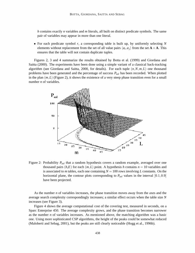
Figures 2, 3 and 4 summarize the results obtained by Botta et al. (1999) and Giordana andSaitta (2000). The experiments have been done using a simple variant of a classical back-trackingalgorithm (see Giordana and Saitta, 2000, for details). For each tuple(n,N,m,L) one thousandproblems have been generated and the percentage of successPsol has been recorded. When plottedin the plan(m,L) (Figure 2), it shows the existence of a very steep phase transition even for a smallnumbern of variables.

Figure 2: ProbabilityPsol that a random hypothesis covers a random example, averaged over onethousand pairs(h,E) for each(m,L) point. A hypothesish containsn = 10 variables andis associated tom tables, each one containingN = 100 rows involvingL constants. On thehorizontal plane, the contour plots corresponding toPsol values in the interval[0.1,0.9]have been projected.

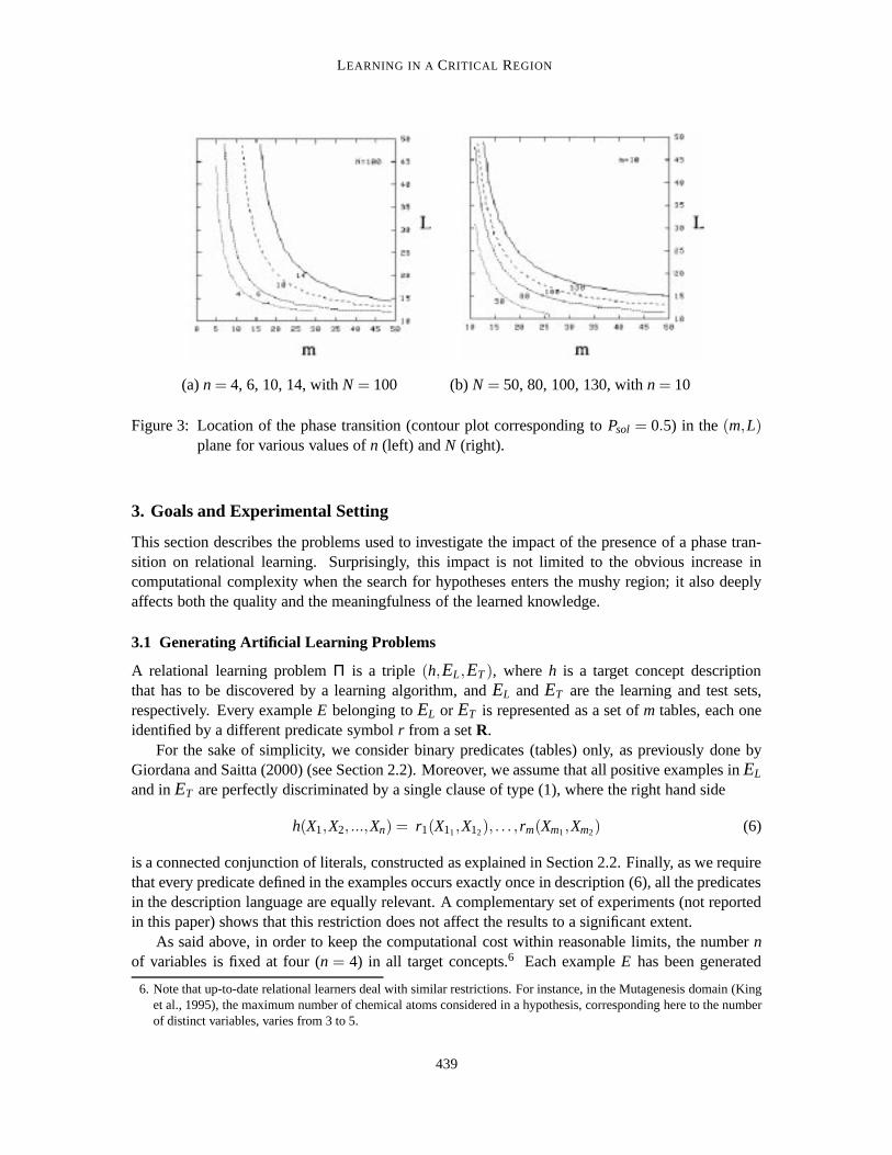
As the numbern of variables increases, the phase transition moves away from the axes and theaverage search complexity correspondingly increases; a similar effect occurs when the table sizeNincreases (see Figure 3).

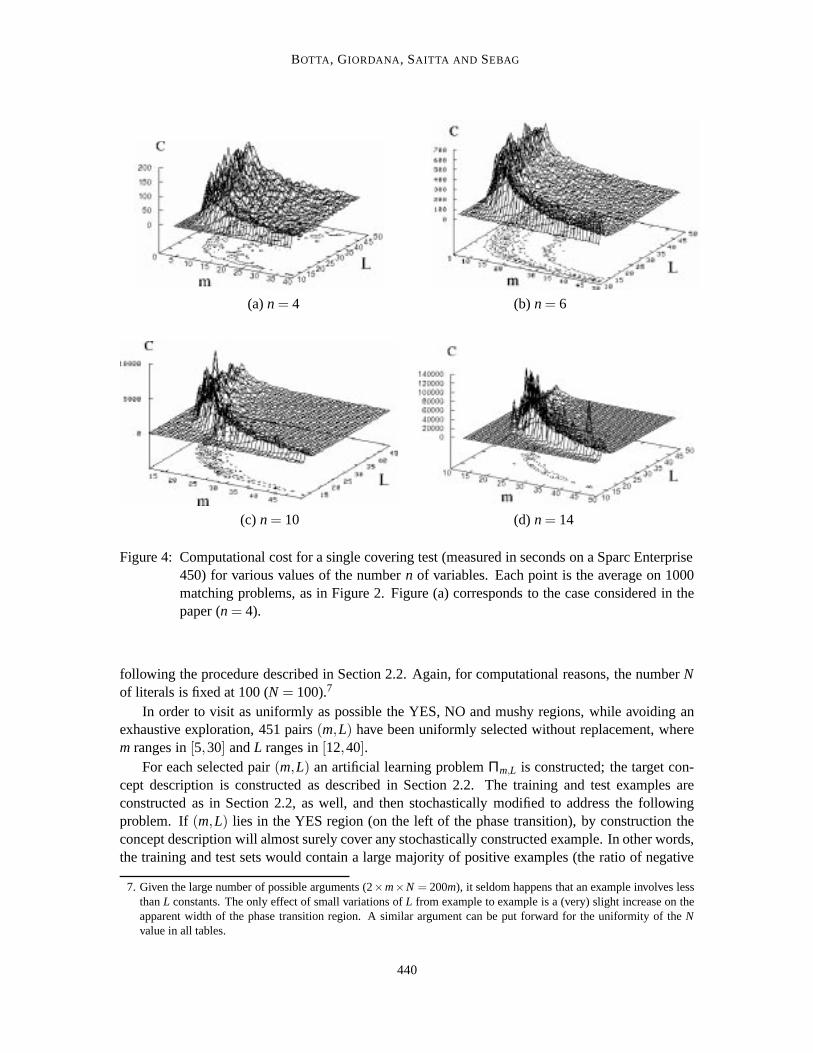
Figure 4 shows the average computational cost of the covering test, measured in seconds, on aSparc Enterprise 450. The average complexity grows, and the phase transition becomes narroweras the numbern of variables increases. As mentioned above, the matching algorithm was a basicone. Using more sophisticated CSP algorithms, the height of the peaks could be somewhat reduced(Maloberti and Sebag, 2001), but the peaks are still clearly noticeable (Hogg et al., 1996b).

438


(a)n = 4, 6, 10, 14, withN = 100 (b)N = 50, 80, 100, 130, withn = 10

Figure 3: Location of the phase transition (contour plot corresponding toPsol = 0.5) in the(m,L)plane for various values ofn (left) andN (right).

3. Goals and Experimental Setting

This section describes the problems used to investigate the impact of the presence of a phase tran-sition on relational learning. Surprisingly, this impact is not limited to the obvious increase incomputational complexity when the search for hypotheses enters the mushy region; it also deeplyaffects both the quality and the meaningfulness of the learned knowledge.

3.1 Generating Artificial Learning Problems

A relational learning problemΠ is a triple (h,EL,ET), whereh is a target concept descriptionthat has to be discovered by a learning algorithm, andEL and ET are the learning and test sets,respectively. Every exampleE belonging toEL or ET is represented as a set ofm tables, each oneidentified by a different predicate symbolr from a setR.

For the sake of simplicity, we consider binary predicates (tables) only, as previously done byGiordana and Saitta (2000) (see Section 2.2). Moreover, we assume that all positive examples inEL

and inET are perfectly discriminated by a single clause of type (1), where the right hand side

h(X1,X2, ...,Xn) = r1(X11,X12), . . . , rm(Xm1,Xm2) (6)

is a connected conjunction of literals, constructed as explained in Section 2.2. Finally, as we requirethat every predicate defined in the examples occurs exactly once in description (6), all the predicatesin the description language are equally relevant. A complementary set of experiments (not reportedin this paper) shows that this restriction does not affect the results to a significant extent.

As said above, in order to keep the computational cost within reasonable limits, the numbernof variables is fixed at four (n = 4) in all target concepts.6 Each exampleE has been generated

6. Note that up-to-date relational learners deal with similar restrictions. For instance, in the Mutagenesis domain (Kinget al., 1995), the maximum number of chemical atoms considered in a hypothesis, corresponding here to the numberof distinct variables, varies from 3 to 5.

439


(a)n = 4 (b) n = 6

(c) n = 10 (d)n = 14

Figure 4: Computational cost for a single covering test (measured in seconds on a Sparc Enterprise450) for various values of the numbern of variables. Each point is the average on 1000matching problems, as in Figure 2. Figure (a) corresponds to the case considered in thepaper (n = 4).

following the procedure described in Section 2.2. Again, for computational reasons, the numberNof literals is fixed at 100 (N = 100).7

In order to visit as uniformly as possible the YES, NO and mushy regions, while avoiding anexhaustive exploration, 451 pairs(m,L) have been uniformly selected without replacement, wherem ranges in[5,30] andL ranges in[12,40].

For each selected pair(m,L) an artificial learning problemΠm,L is constructed; the target con-cept description is constructed as described in Section 2.2. The training and test examples areconstructed as in Section 2.2, as well, and then stochastically modified to address the followingproblem. If(m,L) lies in the YES region (on the left of the phase transition), by construction theconcept description will almost surely cover any stochastically constructed example. In other words,the training and test sets would contain a large majority of positive examples (the ratio of negative

7. Given the large number of possible arguments (2×m×N = 200m), it seldom happens that an example involves lessthanL constants. The only effect of small variations ofL from example to example is a (very) slight increase on theapparent width of the phase transition region. A similar argument can be put forward for the uniformity of theNvalue in all tables.

440


versuspositive examples is 1 to 106 or higher). Symmetrically, if(m,L) lies in the NO-region (onthe right of the phase transition), the training and test sets would contain a large majority of negativeexamples.

However, it is widely acknowledged that ill-balanced datasets make learning considerably moredifficult. As this additional difficulty might blur the results and their analysis, we construct balancedtraining and test sets, each consisting of 100 positive and 100 negative examples. The examplegenerator is then modified; a repair mechanism is added to ensure the fair distribution of the trainingand test sets for learning problems lying outside the phase transition region. As a consequence, thegeneration of the examples proceeds as follows.

Function Problem Generation(m,L)

Construct a descriptionh with m literals of conceptc.EL = DataGeneration(m,L,h).ET = DataGeneration(m,L,h).ReturnΠ = (h,EL,ET).

Function Data Generation(m,L,h)

nb positive = 0, nbnegative = 0Let E = /0while nb positive< 100 or nbnegative< 100do

Generate a random exampleE

if E is covered byh thenif nb positive= 100 then

E = ChangeToNegative(h, E)Set label = NEG

elseSet label = POSelse

if negative= 100 thenE = ChangeToPositive(h, E)Set label = POS

elseSet label = NEGE = E ∪{ (E,label) }if label = POSthen nb positive = nbpositive + 1

elsenb negative = nbnegative + 1endReturnE .

Function ProblemGeneration first constructs a descriptionh of the target conceptc; then, thetraining and test sets are built by the function DataGeneration. The latter accumulates examplesconstructed with the stochastic procedure described in Section 2. When the maximum numberof positive (respectively, negative) examples is reached, further examples are repaired using theChangeToNegative (respectively, ChangeToPositive) function, to ensure that the training and testsets are well balanced. Function ChangeToPositive turns a negative exampleE into a positive one,

441


by inserting into its tables a proper set of tuples, satisfying the conditions set inh, randomly selectedin the spaceA4.

Function ChangeToPositive(h, E)

Uniformly select four constants,a1,a2,a3,a4, from A.Let θ denote the substitutionθ = {X1/a1, X2/a2, X3/a3, X4/a4}for each literal rk(Xi,Xj) in h, do

if tuple〈ai ,aj〉 does not already occur in tablerk of E thenselect randomly and uniformly a tuple occurring in tablerk

and replace it by〈ai ,aj〉endReturnE.

Conversely, function ChangeToNegative modifiesE in order to prevent it from being coveredby h. Let θ = {X1/a1, X2/a2, X3/a3, X4/a4} be a substitution verifyingh in an exampleE. Let(Xj/aj) (2≤ j ≤ 3)8 be the j-th element ofθ, and letrk(Xi,Xj) be one of the literals inh. In orderto falsify h(a1,a2,a3,a4) in E it is sufficient to delete tuple〈ai ,aj〉, from the table associated tork.Unfortunately, this would decrease the numberN of tuples in a table. To avoid this problem it issufficient to add a new tuple (in substitution of〈ai ,aj〉) that is guaranteed not to satisfyh. This isdone in either one of two alternative ways. First, we search for a constanta′j that does not occur inthe left column of the tables associated to the literals where variableXj occurs on the left hand side.If such construct exists, tuple〈ai ,aj〉 is replaced with〈ai ,a′j〉. Otherwise,〈ai ,aj〉, is replaced with atuple already existing in the table ofrk but selected among the ones that do not contribute to satisfyh.9

Function ChangeToNegative(h, E)

Build the setΘ of all substitutions{X1/a1, X2/a2, X3/a3, X4/a4} such that〈a1,a2,a3,a4〉satisfieshwhile Θ is not emptydoRandomly select an atomrk(Xj ,Xi) in hReplace〈aj ,ai〉 in tablerk with a new tuple〈a′j ,a′i〉

such that the number of alternative ways in whichh is satisfied decreasesRecomputeΘendReturnE.

3.2 The Learners

Three learning strategies have been considered: a top-down depth-first search, a top-down beamsearch, and a genetic algorithm based search.

Most learning experiments presented in this paper have been done using the top-down learnerFOIL (Quinlan, 1990), which outputs a disjunction of conjunctive partial hypotheses. FOIL starts

8. As the constants are associated to “chained” variables, in order to falsifyh(a1,a2,a3,a4), it is sufficient to considerthe variables internal to the chain.

9. Notice that, in this case, the tuple distribution in the tables may be modified. However, this happens very rarely andonly whenL is small, so that the influence on the results is irrelevant.

442


with the most general hypothesis, and iteratively specializes the current hypothesisht by adding toits body the “best” conjunctrk(Xi,Xj), according to some evaluation criterion, such as Informationgain (Quinlan, 1990, 1986) or minimum description length (MDL) (Rissanen, 1978). When anyspecialization able to improveht can be found, the latter is retained, all positive examples coveredby ht are removed from the training set, and the search is restarted, unless the training set is empty.The final hypothesish returned by FOIL is the disjunction of all the partial hypothesesht .

Another top-down learner, SMART+ (Botta and Giordana, 1993), has also been used. The maindifference between FOIL and SMART+ resides in their search strategies; FOIL basically uses ahill-climbing search strategy, whereas SMART+ uses a beam search strategy with a user-suppliedbeam width.

m

L

3L

2L

1L

m m m1 2 3

Inductive search path

tc1

)ε1

, L( ε

1,

T

tc2

)ε2

, L( ε2

, T

tc3

)ε3

, L( ε

3,

T

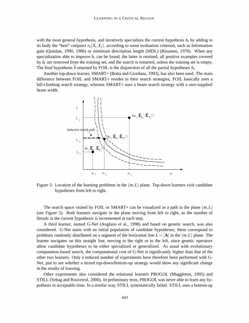
Figure 5: Location of the learning problems in the(m,L) plane. Top-down learners visit candidatehypotheses from left to right.

The search space visited by FOIL or SMART+ can be visualized as a path in the plane(m,L)(see Figure 5). Both learners navigate in the plane moving from left to right, as the number ofliterals in the current hypothesis is incremented at each step.

A third learner, named G-Net (Anglano et al., 1998) and based on genetic search, was alsoconsidered. G-Net starts with an initial population of candidate hypotheses; these correspond toproblems randomly distributed on a segment of the horizontal lineL = |A| in the(m,L) plane. Thelearner navigates on this straight line, moving to the right or to the left, since genetic operatorsallow candidate hypotheses to be either specialized or generalized. As usual with evolutionarycomputation-based search, the computational cost of G-Net is significantly higher than that of theother two learners. Only a reduced number of experiments have therefore been performed with G-Net, just to see whether a mixed top-down/bottom-up strategy would show any significant changein the results of learning.

Other experiments also considered the relational learners PROGOL (Muggleton, 1995) andSTILL (Sebag and Rouveirol, 2000). In preliminary tests, PROGOL was never able to learn any hy-pothesis in acceptable time. In a similar way, STILL systematically failed. STILL uses a bottom-up

443


approach, based on the stochastic (uniform or biased) sampling of the matchings between a hypoth-esis and the examples. Its failure is due to the uniform construction of the examples and the lack ofany domain bias.

3.3 Discussion

Let us summarize here all simplifications and assumptions. Some of them should facilitate thesearch (legend+), while others rather hinder relational learning (legend−):

+ There are no constants in the target concept and no variables in the examples.

+ The training and test sets are equally distributed (100 positive and 100 negative examples),without any noise.

+ All target concepts are conjunctive: a single hypothesish covers all positive examples andrejects all negative ones.

+ Both target concept and examples are single definite clauses.

+ All predicates in the examples are relevant: they all appear in the target concept. No otherbackground knowledge is given to the learner.

+ variables in the description of the target concept are chained.

− All examples have the same size (N times the number of predicate symbols in the targetconcept).

− All tables (predicate definitions) have the same number of rows in every example.

− All predicates are binary.

− All predicate arguments have the same domain of values.

Let us notice that, even if the structure of the target concept (m literals involvingn= 4 variables)were known by the learners (which is obviously not the case), the size of the search space (42m)prevents the solution being discovered by chance. Moreover, given the descriptionh of c, thelearning task amounts to finding the right bindings among the 2×m arguments involved in thembinary predicates, i.e., partitioning the 2m arguments into four subsets.

3.4 Goal of the Experiments

In order to investigate the impact of the phase transition on relational learning, our goal is to assessthe behavior of all considered learners depending on the position of learning problems with respectto the phase transition. The behavior of each learner is examined with regards to three specificcriteria:

• Predictive accuracy. The accuracy is commonly measured by the percentage of test exam-ples correctly classified by the hypothesish produced by the learner.10 The accuracy is con-sidered satisfactory if and only if it is greater than 80% (the issue of choosing this thresholdvalue will be discussed later).

10. The predictive accuracy was not evaluated according to the usual cross-validation procedure for two reasons. First ofall, the training and test sets are drawn from the same distribution; it is thus equivalent to doubling the experiments

444


• Concept identification. It must be emphasized that a high predictive accuracy doesnotimply that the learner has discovered the true target concept. The two issues must thereforebe distinguished. The identification is considered satisfactory if and only if the structure ofhis close to that of the true target concept, i.e., ifh is conjunctive with the same size ash.

• Computational cost. The computational cost reflects both the total number of candidatehypotheses considered by the learner, and the cost of assessing each of them on the trainingset. Typically, the more candidate hypotheses in the phase transition region, the higher thecomputational cost.

4. Results

This section reports the results obtained by FOIL, SMART+ and G-Net on the artificial relationallearning problems constructed as previously described.

4.1 Predictive Accuracy

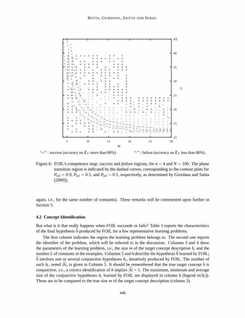
Figure 6 summarizes the results obtained by FOIL with respect to predictive accuracy. As mentionedearlier, 451 pairs(m,L) have been chosen in order to explore significant parts of the YES, mushy,and NO regions. For each selected pair(m,L) a learning problemΠm,L = (h, EL, ET) has beenconstructed, wherem is the number of literals inh andL the number of constants in the training/testexamples.

On each problem, FOIL either succeeds (legend “+”, indicating that the predictive accuracy onthe test set is greater than 80%), or fails (legend “·”).

Let us first comment on the significance of these results, with respect to the success thresholdand the learning strategy. First, the shape of the failure region (the “blind spot”) is almost inde-pendent of the threshold used to define a failure case (predictive accuracy on the test set lowerthan 80%). In a vast majority of cases, the hypothesesh learned by FOIL are either very accurate(predictive accuracy close to 100%), or comparable to a random guess (predictive accuracy close to50%). The threshold could thus be any value between 95% and 60%, without making any significantdifference in the shape of the blind spot.

Regarding the mere learning performances, it appears that FOIL succeeds mainly in two cases:either when the target concept is simple (for low values ofm), or when the learning problem is far(to the right) from the phase transition region.

The first case is hardly surprising; the simpler the target concept, the easier learning should be.Much more unexpected is the fact that learning problems far to the right of the phase transitionappear to be easier to solve. In particular, the fact that increasing the number of constants11 inthe application domainfacilitatesrelational learning (everything else being equal, i.e., for the sametarget concept size), is counter-intuitive. Along the same lines, it is counter-intuitive that increasingthe sizem of the target concept might facilitate relational learning (everything else being equal

and taking the average result, or performing a twofold cross-validation (Dietterich, 1998). We did not double theexperiments because of the huge total computational cost. Moreover, though the learning result obtained for(m,L)is based on a single trial, it might be considered significant to the extent that other trials done in the same area givethe same result.

11. Note that form> 6 the learning problem moves away from the phase transition asL increases.

445


++++...........+.++

+

++

+

+++........

.

.++

++++++

++++

.

.

.

.

.

.

.

.

.

.

+.+++.

+

+++++

+..

.

.

.

.

.

.

+

+.+++

++

+

.

.

.

.

.

.

.

.+

.

.++++++++++

+

.

.

.

.

.

.

.

.

.

.

.

.++++

+++.

+++

+..

.

.

.

.

.

.+

+++++

+

+

+++.+

+.....

.

++

+++++

++++++

+

.

.

.

.

.

.

.

.

.

+++++

.

++++++

.

.

.

.

.

.

.+...++.+++++++

++

+......+.++++

.

.

.

.

.

.

.++...

.

.

.

.

.

.

.

.++++

.

.

.

.

.

.

.+...++

.

.

.

.

.

.

.

.+++++

.

.

.

.

.

++

+++

.

.

.

.

.

.

.

.

.+++

.

.

.

.

.

.

.

.

.+.++

.

.

.

.

.

.+++

.++

.

.

.

.

.+....

++

+++++

++++

++

+

+++++++++

+

+

+

+++

.++++.+

.+++++++.

++

+++

++.

+....++

.+++.

++

+

++..

.

.

.

.+.+...+.++

++

+

++.......+.

.

.+

++++++.+

5 10 15 20 25 30

m

10

15

20

25

30

35

40

45

L

“+” : success (accuracy onET more than 80%) “·” : failure (accuracy onET less than 80%).

Figure 6: FOIL’s competence map:successandfailure regions, forn = 4 andN = 100. The phasetransition region is indicated by the dashed curves, corresponding to the contour plots forPsol = 0.9, Psol = 0.5, andPsol = 0.1, respectively, as determined by Giordana and Saitta(2000)).

again, i.e., for the same number of constants). These remarks will be commented upon further inSection 5.

4.2 Concept Identification

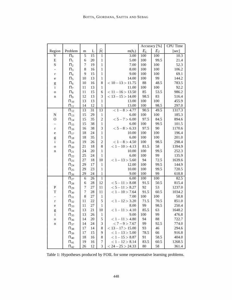
But what is it that really happens when FOIL succeeds or fails? Table 1 reports the characteristicsof the final hypothesish produced by FOIL for a few representative learning problems.

The first column indicates the region the learning problem belongs to. The second one reportsthe identifier of the problem, which will be referred to in the discussion. Columns 3 and 4 showthe parameters of the learning problem, i.e., the sizem of the target concept descriptionh, and thenumberL of constants in the examples. Columns 5 and 6 describe the hypothesish learned by FOIL;h involves one or several conjunctive hypothesesht , iteratively produced by FOIL. The number ofsuchht , noted|h|, is given in Column 5. It should be remembered that the true target concepth isconjunctive, i.e., a correct identification ofh implies |h| = 1. The maximum, minimum and averagesize of the conjunctive hypothesesht learned by FOIL are displayed in column 6 (legendm(ht )).These are to be compared to the true sizem of the target concept description (column 3).

446


The last three columns report the predictive accuracy ofh on the training and test set, and thetotal CPU time required by FOIL to complete the learning task, measured in seconds on a SparcEnterprise 450. The learning problems in Table 1 can be grouped into three categories:

• Easyproblems, which are correctly solved; FOIL finds a conjunctive hypothesish that accu-rately classifies (almost) all training and test examples. Furthermore,h is identical to the trueconcept descriptionh, or differs by at most one literal. Problems of this type areΠ0 to Π5,Π7, Π10, Π11, Π27 andΠ31. Most easy problems lie in the YES region; some others lie inthe mushy region for low values ofm (m≈ 6).

• Feasibleproblems, which are efficiently solved, even though the correct target concept de-scription is not found. More precisely, FOIL learns a concept descriptionh which (a) ispredictively accurate (nearly all training and test examples are correctly classified), (b) con-sists of a single conjunctive hypothesis, as the original target concept descriptionh, and (c)shares many literals withh. However,h is significantly shorter thanh (e.g., h involves 9literals versus 29 inh for problemΠ26); in many cases,h largely over-generalizesh. Mostfeasible problems lie in the NO-region, rather far away from the phase transition. Problemsof this kind areΠ13, Π15, Π17, Π18, Π21, Π22, Π24 to Π26, Π33 andΠ35.

• Hard problems, which are not solved by FOIL. The learned concept descriptionh is thedisjunction of many conjunctive hypothesesht (between 6 and 15) of various sizes, and eachht covers only a few training examples. From a learning perspective, over-fitting has occurred(eachht behaves well on the training set, but its accuracy on the test set is comparable to thatof random guessing), related to an apparentsmall disjunctsproblem (Holte et al., 1989). Hardproblems lie in the PT region or in the NO region, but, in contrast to feasible problems, closeto the phase transition.

These results confirm that predictive accuracy may be related only loosely to the discovery of thetrue concept.

It is clear that in real-world problems there is no way distinguishing between feasible and easyproblems, since the true concept is unknown. Again, we shall return to this point later on. Asummary of the average results obtained in the YES, NO and PT regions (Table 2) shows that mosthard problems are located in the mushy region; conversely, most problems in the PT region are hard.

A second remark concerns the location of the hypothesesht learned by FOIL. It is observedthat for all learning problems, except the easy ones located in the YES region,all hypotheses ht lieinside the phase transition region(see Figure 7). This is the case no matter whether FOIL discoversone or several conjunctive hypothesesht , and whatever the location of the learning problem, lyingin the mushy or in the NO region. More precisely:

– when the target concept lies in the mushy region and the problem is easy, FOIL correctlydiscovers the true concept;

– for feasible learning problems, FOIL discovers a generalization of the true concept, which liesin the mushy region; and

– for hard problems, FOIL retains several seemingly randomht ’s, most of which belong to themushy region.

As previously noted by Giordana and Saitta (2000), the phase transition does behave as anattractor for the learning search. Interpretations of this finding will be discussed in Section 5.

447


Accuracy [%] CPU TimeRegion Problem m L |h| m(ht) EL ET [sec]

Y Π0 5 15 1 3.00 100 100 10.3E Π1 6 20 1 5.00 100 99.5 21.4S Π2 7 19 1 7.00 100 100 52.3- Π3 8 16 1 8.00 100 100 106.2r Π4 9 15 1 9.00 100 100 69.1e Π5 10 13 1 14.00 100 99 144.2g Π6 10 16 8 < 10−13> 11.75 88 48.5 783.5i Π7 11 13 1 11.00 100 100 92.2o Π8 11 15 6 < 11−16> 13.50 85 53.5 986.2n Π9 12 13 3 < 13−15> 14.00 98.5 83 516.4

Π10 13 13 1 13.00 100 100 455.9Π11 14 12 1 13.00 100 98.5 297.0Π12 13 31 13 < 1−8> 4.77 90.5 49.5 1317.3

N Π13 15 29 1 6.00 100 100 185.3O Π14 15 35 2 < 5−7> 6.00 97.5 84.5 894.6- Π15 15 38 1 6.00 100 99.5 101.5r Π16 16 38 3 < 5−8> 6.33 97.5 90 1170.6e Π17 18 24 1 10.00 100 100 196.4g Π18 18 35 1 6.00 100 100 201.0i Π19 19 26 2 < 1−8> 4.50 100 98.5 298.4o Π20 21 18 8 < 1−10> 4.13 81.5 58 1394.9n Π21 24 20 1 10.00 100 99.5 252.3

Π22 25 24 1 6.00 100 99 135.9Π23 27 18 10 < 1−13> 5.60 94 72.5 1639.6Π24 29 17 1 12.00 100 99.5 144.9Π25 29 23 1 10.00 100 99.5 720.5Π26 29 24 1 9.00 100 99 618.8Π27 6 26 1 6.00 100 100 82.5Π28 6 28 12 < 5−11> 8.08 91.5 50.5 815.4

P Π29 7 27 11 < 5−11> 8.27 92 53 1237.0T Π30 7 28 11 < 1−10> 7.64 91.5 60.5 1034.2- Π31 8 27 1 7.00 100 100 58.8r Π32 11 22 5 < 1−12> 3.20 71.5 70.5 851.0e Π33 11 27 1 8.00 99 98.5 250.4g Π34 13 21 10 < 1−11> 4.10 85.5 63 1648.2i Π35 13 26 1 9.00 100 99 476.8o Π36 14 20 5 < 1−11> 4.80 94 88 722.7n Π37 14 24 3 < 7−9> 7.67 99 92.5 774.0

Π38 17 14 8 < 13−17> 15.00 93 46 294.6Π39 17 15 9 < 1−13> 5.00 78.5 66 916.8Π40 18 16 8 < 1−15> 8.87 91 58.5 404.0Π41 19 16 7 < 1−12> 8.14 83.5 60.5 1268.5Π42 26 12 3 < 24−25> 24.33 80 58 361.4

Table 1: Hypotheses produced by FOIL for some representative learning problems.

448


Region Nb of Pbs Percentage of Average nb of hyp. Avg on solved pbspbs solved pbs solved pbs unsolved Test acc. CPU time

YES 46 88.1% (37) 1 6.33 99.61 74.05NO 195 72.8% (142) 1.27 8.28 99.61 385.43PT 210 28.1% (59) 1.10 8.18 99.12 238.25

Total 451 52.8% (238) 1.12 7.60 99.45 232.58

Table 2: Summary of the experiments. Easy and feasible learning problems (Solved Pbs) are dis-tinguished from hard problems (Unsolved Pbs).

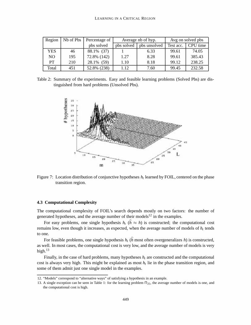
Figure 7: Location distribution of conjunctive hypothesesht learned by FOIL, centered on the phasetransition region.

4.3 Computational Complexity

The computational complexity of FOIL’s search depends mostly on two factors: the number ofgenerated hypotheses, and the average number of their models12 in the examples.

For easy problems, one single hypothesisht (h ≈ h) is constructed; the computational costremains low, even though it increases, as expected, when the average number of models ofht tendsto one.

For feasible problems, one single hypothesisht (h most often overgeneralizesh) is constructed,as well. In most cases, the computational cost is very low, and the average number of models is veryhigh.13

Finally, in the case of hard problems, many hypothesesht are constructed and the computationalcost is always very high. This might be explained as mostht lie in the phase transition region, andsome of them admit just one single model in the examples.

12. “Models” correspond to “alternative ways” of satisfying a hypothesis in an example.13. A single exception can be seen in Table 1: for the learning problemΠ25, the average number of models is one, and

the computational cost is high.

449


Everything else being equal, the learning cost is higher for problems in the NO region. One forthis higher complexity is the size of the hypothesis space, which exponentially increases with thenumberm of literals in h; this causes many more hypotheses to be considered and tested in eachlearning step. Another cause is that the NO region includes many hard problems (see Figure 6); onsuch problems, the PT region is visited again and again because many hypotheses are tried.

4.4 Comparison to other Learning Algorithms

The results presented so far have been obtained by FOIL. A natural question arises about the biasof the specific learner employed.

In order to explore this issue, SMART+ and G-Net have been tested on the learning problemsreported in Figure 6. SMART+ uses a beam search strategy so that the system runs slower thanFOIL in proportion to the size of the beam. G-Net uses an elitist genetic algorithm, which repeatsa cyclic procedure that, at every iteration, explores a new inductive hypothesis, until it convergesto a stable solution. On the considered set of learning problems, a stable solution is reached onlyafter many thousands of iterations. As each iteration requires testing the newly created hypothesison the whole learning set, G-Net’s computational time is heavily affected by the presence of thecomplexity peak in the mushy region. In the present experiments, the number of iterations has beenfixed to 50,000 for all runs. With this setting, the CPU time may range from several hours to severaldays for a single problem.

Thus, due to the high computational cost, the comparison has been restricted to the subset ofproblems reported in Table 1. The results are reported in Table 3. It appears that FOIL and SMART+are discordant on 7 problems out of 43, in the sense that the same problem has been solved by oneof the algorithms but not by the other. Nevertheless, such problems appear to be on the border ofthe blind spot (see Figure 6), where FOIL itself alternates successes and failures.

On all the other cases, there is a substantial agreement. In all runs the beam width of SMART+has been fixed to 5. Increasing the width of the beam and granting very large computational re-sources, SMART+ can solve a few more problems. However, it is unrealistic to use this approachsystematically. On the other hand, G-Net solved fewer problems than the other two systems. Infact, G-net would need a higher number of iterations in order to converge, but this was prohibitivebecause of the computational complexity. Tuning G-Net control parameters did not bring any sig-nificant improvement.

SMART+ has also been applied to other problems (about 100) sampled randomly inside andoutside the blind spot, but far from the borders; in all cases successes and failures have been inagreement with FOIL.

5. Interpretation

This section proposes an interpretation of the results reported so far. The discussion focuses onthree main questions: why is the learning search captured by the PT region? When and why doesrelational learning miss the true target concept? When and why should relational learning fail tofind any accurate approximation of the target concept?

450


SMART+ G-NETAccuracy [%] CPU Time Accuracy [%]

Region Problem m L |h| m(ht ) EL ET [sec] |h| m(ht ) EL ETY Π0 5 15 1 3 100 99 130 1 3 100 99E Π1 6 20 1 6 100 99.5 429 1 5 100 99.5S Π2 7 19 1 7 99.5 100 667 21 9 100 73.5- Π3 8 16 1 8 100 100 218 14 12 100 74r Π4 9 15 1 9 100 100 99 13 16 100 67e Π5 10 13 1 10 100 100 609 1 16 100 98g Π6 10 16 - - - - 1305 21 12 100 58.5i Π7 11 13 1 11 100 100 509 2 12 100 94.5o Π8 11 15 - - - - 592 22 18 100 50.5n Π9 12 13 - - - - 418 1 10 100 95

Π10 13 13 1 13 100 100 3368 24 12 100 48.5Π11 14 12 1 14 100 100 1935 1 13 100 98.5Π12 13 31 1 8 96.5 98 626 1 7 100 100

N Π13 15 29 1 7 99.5 100 1081 34 6 100 55.5O Π14 15 35 4 7 100 97.5 743 29 6 100 68- Π15 15 38 11 8 100 98 882 36 6 100 60r Π16 16 38 2 7 98.5 100 514 1 6 100 99e Π17 18 24 1 9 100 99.5 1555 28 8 100 54.5g Π18 18 35 1 7 96 99 590 1 6 99.5 98.5i Π19 19 26 8 8 100 99.5 1410 33 7 100 53o Π20 21 18 1 12 100 99.5 2396 22 10 100 47.5n Π21 24 20 10 10 99 93 2034 27 8 100 52

Π22 25 24 1 8 99 99.5 2331 30 6 99.5 57.5Π23 27 18 1 10 100 97 3289 26 13 96.5 50.5Π24 29 17 24 12 97.5 75 7004 27 11 100 53Π25 29 23 1 9 100 99.5 2241 35 8 100 46.5Π26 29 24 2 9 100 100 2887 30 8 97 51Π27 6 26 - - - - - 17 9 99 86Π28 6 28 1 6 97.5 100 932 34 8 100 51.5

P Π29 7 27 - - - - - 42 7 100 50.5T Π30 7 28 1 7 98.5 100 396 32 8 100 57- Π31 8 27 5 8 99 93.5 640 19 8 100 81.5r Π32 11 22 - - - - - 30 8 100 50e Π33 11 27 - - - - - 37 7 100 54.5g Π34 13 21 - - - - - 33 7 99 49.5i Π35 13 26 1 8 98.5 98 864 1 7 100 100o Π36 14 20 - - - - - 29 9 100 44.5n Π37 14 24 - - - - - 32 8 100 59

Π38 17 14 - - - - 4371 24 15 100 47.5Π39 17 15 - - - - - 21 15 97 56Π40 18 16 25 14 96 53 24172 24 13 100 46Π41 19 16 - - - - - 21 13 100 52.5Π42 26 12 - - - - 14273 29 10 99.5 47

Table 3: Hypotheses produced by SMART+ and G-Net for the same learning problems reported inTable 1. Smart+ uses beam search, and the beam width was set to 5. Symbol ’-’, meansthat the learning process reached the maximum allowed time of 6 hours, without finding asolution. G-Net always run for a number of iterations fixed to 50,000.

5.1 Why the Phase Transition Attracts the Learning Search

Being a top-down learner, FOIL constructs a series of increasingly specific candidate hypotheses,h1, . . . ,ht . The earlier hypotheses in the series belong to the YES region by construction.

If the most specific hypothesishi built up in the YES region is not satisfactory according to thestop criterion (see below), FOIL moves into the PT region, andhi+1 belongs to it. It might alsohappen that the most specific hypothesishj ( j > i) in the PT region is not satisfactory either; FOILthen comes to visit the NO region.

Let us consider the stop criterion used in FOIL. The search is stopped when the current hypoth-esis issufficiently correct, covering no or few negative examples; on the other hand, at each step, thecurrent hypothesis is required to besufficiently complete, covering asufficient numberof positiveexamples. The implications of these criteria are discussed, depending on the location of the targetconcept descriptionh with respect to the phase transition.

451


Case 1: h belongs to the PT region.By construction, the target concept descriptionh covers with probability close to 0.5 any randomexample (Section 2.2); therefore, the repair mechanism that ensures the dataset is balanced is notemployed (Section 3.1). It follows that:

• Since any hypothesis in the YES region almost surely covers any random example, it almostsurely covers all training examples, both positive and negative. Therefore the searchcannotstopin the YES region, but must proceed to visit the PT region.

• Symmetrically, any hypothesis in the NO region almost surely rejects (does not cover) anyrandom example; then, almost surely, it will cover no training examples at all. Although thesehypotheses are correct, they are too incomplete to be acceptable. Therefore, the search muststop before reaching the NO region. As a consequence, FOIL is bound to produce hypothesesht lying in the PT region.

Case 2: h belongs to the NO region.In this case, randomly constructed examples are almost surely negative (see Section 3.1). It followsthat any hypothesis in the YES region will almost surely cover the negative examples; this impliesthat the search cannot stop in the YES region. On the other hand, any hypothesis in the NO regionwill almost surely be correct (covering no negative examples); therefore, there is no need for FOILto go deeply into the NO region. Hence, FOIL is bound to produce hypothesesht lying in the PTregion, or on the verge of the NO region.

Case 3: h belongs to the YES region.The situation is different here, since there exist correct hypotheses in the YES region, namely thetarget concept itself and possibly many other hypotheses more specific than it. Should these hy-potheses be discovered (the chances for such a discovery are discussed in the next subsection), thesearch could stop immediately. But in all cases, the search must stop before reaching the NO re-gion, for the following reason. Ash belongs to the YES region, randomly constructed examples arealmost surely positive examples (see Section 3.1). This implies that any hypothesis in the NO re-gion will almost surely reject the positive examples, and will therefore be considered insufficientlycomplete. In this case again, FOIL is bound to produce hypothesesht in the YES region or in thePT region.

In conclusion, FOIL is unlikely to produce hypotheses in the NO region, whatever the locationof the target concept descriptionh is, at least when the negative examples are uniformly distributed.Most often, FOIL will produce hypotheses belonging to the PT region, but it might produce ahypothesis in the YES region ifh itself belongs to it. It is worth noting that such a behavior has alsobeen detected in several real-world learning problems (see Giordana and Saitta, 2000).

Analogous considerations hold for SMART+, and, more generally, for any top-down learner:as maximally general hypotheses are preferred, provided that they are sufficiently discriminating,searching in the NO region does not bring any benefit. It follows that the phase transitionbehavesas an attractor for any top-down relational learner.

The experiments done with G-Net indicate that the same conclusion also holds for GA-basedlearning, notwithstanding the strong difference between its search strategy and the top-down one.The explanation offered for this finding is the following. The starting point in genetic search (the

452


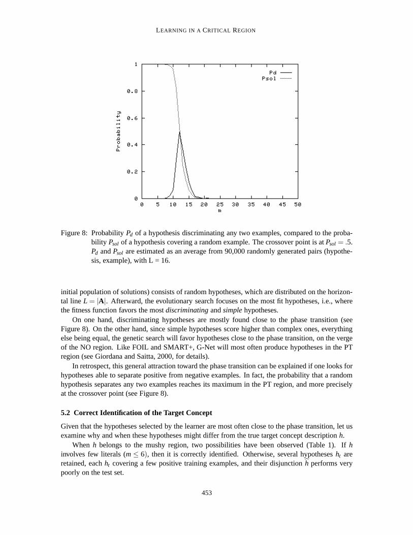
Figure 8: ProbabilityPd of a hypothesis discriminating any two examples, compared to the proba-bility Psol of a hypothesis covering a random example. The crossover point is atPsol = .5.Pd andPsol are estimated as an average from 90,000 randomly generated pairs (hypothe-sis, example), with L = 16.

initial population of solutions) consists of random hypotheses, which are distributed on the horizon-tal line L = |A|. Afterward, the evolutionary search focuses on the most fit hypotheses, i.e., wherethe fitness function favors the mostdiscriminatingandsimplehypotheses.

On one hand, discriminating hypotheses are mostly found close to the phase transition (seeFigure 8). On the other hand, since simple hypotheses score higher than complex ones, everythingelse being equal, the genetic search will favor hypotheses close to the phase transition, on the vergeof the NO region. Like FOIL and SMART+, G-Net will most often produce hypotheses in the PTregion (see Giordana and Saitta, 2000, for details).

In retrospect, this general attraction toward the phase transition can be explained if one looks forhypotheses able to separate positive from negative examples. In fact, the probability that a randomhypothesis separates any two examples reaches its maximum in the PT region, and more preciselyat the crossover point (see Figure 8).

5.2 Correct Identification of the Target Concept

Given that the hypotheses selected by the learner are most often close to the phase transition, let usexamine why and when these hypotheses might differ from the true target concept descriptionh.

When h belongs to the mushy region, two possibilities have been observed (Table 1). Ifhinvolves few literals (m≤ 6), then it is correctly identified. Otherwise, several hypothesesht areretained, eachht covering a few positive training examples, and their disjunctionh performs verypoorly on the test set.

453


r0(X1,X2) r1(X1,X2) r2(X1,X2) r3(X1,X2) r4(X1,X2) r5(X1,X2) r6(X1,X2) r7(X1,X2)

r4(X1,X3)g=246.80

r6(X4,X3)g=1028.28

r5(X1,X3)g=4239.64

r7(X4,X3)g=1071.89

r3(X4,X3)g=1179.06

r2(X1,X4)g=982.56

r1(X2,X4)g=129.24

r0(X3,X1)g=213.73

r4(X3,X4)g=985.66

r5(X3,X4)g=3485.03

r6(X2,X4)g=402.46

r7(X2,X4)g=312.22

r3(X2,X4)g=352.79

r2(X3,X2)g=272.70 1|96)

r5(X1,X3)g=237.78

r0(X1,X4)g=781.96

r4(X1,X3)g=3928.51

r7(X2,X3)g=979.65

r3(X2,X3)g=1010.14

r6(X2,X3)g=1013.87

r1(X4,X2)g=129.24

r1(X3,X1)g=205.21

r0(X4,X3)g=963.29

r7(X1,X2)g=1651.52

r6(X1,X2)g=1355.43

r2(X4,X1)g=225.23

r4(X4,X2)g=320.77

r5(X4,X2)g=378.25

r0(X1,X3)g=246.80

r6(X4,X2)g=1028.28

r5(X1,X2)g=4329.64

r7(X4,X2)g=1071.89

r3(X4,X2)g=1179.06

r2(X1,X4)g=982.56

r1(X3,X4)g=129.24

r2(X1,X3)g=237.78

r0(X1,X4)g=781.96

r4(X1,X2)g=3928.51

r7(X3,X2)g=979.75

r3(X3,X2)g=1010.14

r6(X3,X2)g=1013.87

r1(X4,X3)g=129.24

r1(X3,X1)g=158.13

r0(X4,X3)g=1011.54

r3(X1,X2)g=1294.97

r7(X1,X2)g=1471.76

r2(X4,X1)g=225.23

r4(X4,X2)g=320.77

r5(X4,X2)g=378.25

r4(X3,X2)g=121.57

r0(X3,X4)g=1419.53

r5(X3,X2)g=4563.94

r3(X1,X2)g=1425.26

r6(X1,X2)g=1071.68

r2(X3,X1)g=982.56

r1(X4,X1)g=129.24

r6(X3,X2)g=270.37

r4(X4,X3)g=2179.51

R7(X3,X1)g=1708.79

r1(X3,X2)g=663.91

r1(X4,X2)g=3431.41

r7(X4,X3)g=1220.88

r7(X4,X3)g=490.57

r2(X1,X4)g=1943.96

r7(X3,X1)g=1196.79

r3(X3,X2)g=452.89

r1(X4,X1)g=3366.04

R4(X4,X3)g=1735.84

r5(X2,X1)g=532.38

r4(X3,X2)g=445.87

R7(X2,X1)g=1708.79

r1(X2,X3)g=274.88

r1(X4,X1)g=4328.31

r4(X2,X3)g=296.44

r2(X1,X4)g=1943.96

r7(X2,X1)g=1196.79

R4(X4,X3)g=1573.73

r0(X2,X1)g=1543.87

r5(X2,X1)g=532.38

r0(X3,X1)g=243.30

r4(X4,X2)g=3305.10

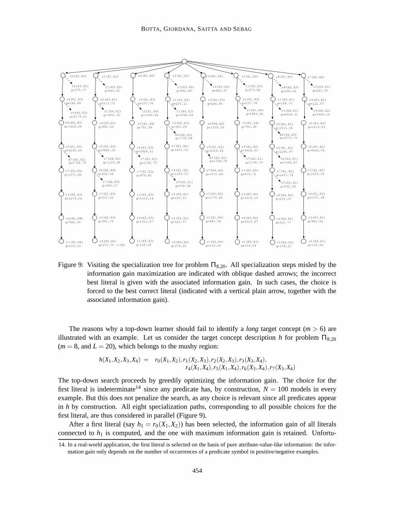
Figure 9: Visiting the specialization tree for problemΠ8,20. All specialization steps misled by theinformation gain maximization are indicated with oblique dashed arrows; the incorrectbest literal is given with the associated information gain. In such cases, the choice isforced to the best correct literal (indicated with a vertical plain arrow, together with theassociated information gain).

The reasons why a top-down learner should fail to identify along target concept (m > 6) areillustrated with an example. Let us consider the target concept descriptionh for problemΠ8,20

(m= 8, andL = 20), which belongs to the mushy region:

h(X1,X2,X3,X4) = r0(X1,X2), r1(X2,X3), r2(X2,X3), r3(X3,X4),r4(X1,X4), r5(X1,X4), r6(X3,X4), r7(X3,X4)

The top-down search proceeds by greedily optimizing the information gain. The choice for thefirst literal is indeterminate14 since any predicate has, by construction,N = 100 models in everyexample. But this does not penalize the search, as any choice is relevant since all predicates appearin h by construction. All eight specialization paths, corresponding to all possible choices for thefirst literal, are thus considered in parallel (Figure 9).

After a first literal (sayh1 = r0(X1,X2)) has been selected, the information gain of all literalsconnected toh1 is computed, and the one with maximum information gain is retained. Unfortu-

14. In a real-world application, the first literal is selected on the basis of pure attribute-value-like information: the infor-mation gain only depends on the number of occurrences of a predicate symbol in positive/negative examples.

454


nately, it turns out that the best literal according to this criterion (e.g.,r6(X3,X2) with gain 270.37)is incorrect, i.e., it is such that hypothesish2 = r0(X1,X2), r6(X3,X2) doesnot generalizeh; hence,the search cannot recover and will fail, unless backtracking is used (see below).

On this particular problem, the maximization of the information gain appears to be seriouslymisleading. In all but one of the eight specialization paths, the first specialization step (regardingthe second literal) fails as FOIL selects incorrect literals (displayed in Figure 9 with a dashed obliquearrow, together with the corresponding information gain value).

When a specialization choice is incorrect, FOIL must either backtrack, or end up with an incor-rect hypothesisht . In order to see the total amount of backtracking needed to find the true targetconcept descriptionh, let us manually correct hypothesish2, and replace the wrong literal selectedwith the best correct literal (literal with maximum information gain such thath2 does generalizethe true target concept). The best correct literal is indicated with a solid vertical arrow in Figure 9,together with the corresponding information gain; clearly, the best correct literal appears to be oftenpoor in terms of information gain.

Unfortunately, it appears that forcing the choice of a correct second literal is not enough; eventhoughh2 is correct, the selection of the third literal is again misled by the information gain criterion,in all branches but one. To pursue the investigation, let us force again the choice of the best correcti-th literal, in all cases where the optimal literal with respect to information gain is not correct. Allrepairs needed are reported in Figure 9.

These considerations show that greedy top-down search is most likely bound to miss the truetarget concept, as there is no error-free specialization path for this learning problem.

5.3 Impact on the Search Strategy

According to Figure 9, a large amount of backtracking would be needed in order to discover thetrue target concept from scratch. More precisely, the information gain appears to be reliable in thelate stages of induction, provided that the current hypothesis is correct (in the case of Figure 9, thesearch needs to be “seeded” with four correct literals). In other words, the information gain criterioncan be used to transform aninformedguess (the first four literals) into an accurate hypothesis, if andonly if the guess has reached some critical size (in the particular case of problemΠ8,20, the criticalsize corresponds to half the size of the true concept).

Let us define the size of the informed guessmk as the minimum number of literals such that,with probability 0.5, FOIL finds the target concept descriptionh, or a correct generalization of it,by refining amk-literal guess.

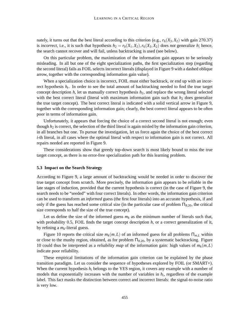
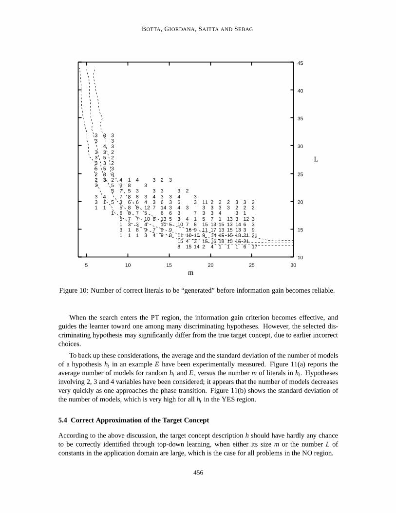
Figure 10 reports the critical sizemk(m,L) of an informed guess for all problemsΠm,L withinor close to the mushy region, obtained, as for problemΠ8,20, by a systematic backtracking. Figure10 could thus be interpreted as areliability map of the information gain: high values ofmk(m,L)indicate poor reliability.

These empirical limitations of the information gain criterion can be explained by the phasetransition paradigm. Let us consider the sequence of hypotheses explored by FOIL (or SMART+).When the current hypothesishi belongs to the YES region, it covers any example with a number ofmodels that exponentially increases with the number of variables inhi , regardless of the examplelabel. This fact masks the distinction between correct and incorrect literals: the signal-to-noise ratiois very low.

455


133

3225333

33

114

33353534

3

1

5

35233222333

13156537734

11378868581

183778683

4

3941051243

3

47

8

7343

3

991013614633

2

89556333

3

81511

10334643

154101674

3

2

143109817

33

2159111553311

4161417137332

1181513151432

11515151313

32

1151813143323

621213612123

17

21933

22

5 10 15 20 25 30

10

15

20

25

30

35

40

45

L

m

Figure 10: Number of correct literals to be “generated” before information gain becomes reliable.

When the search enters the PT region, the information gain criterion becomes effective, andguides the learner toward one among many discriminating hypotheses. However, the selected dis-criminating hypothesis may significantly differ from the true target concept, due to earlier incorrectchoices.

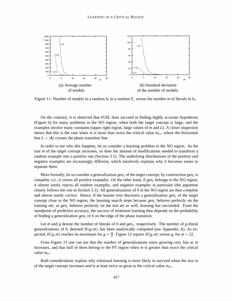
To back up these considerations, the average and the standard deviation of the number of modelsof a hypothesisht in an exampleE have been experimentally measured. Figure 11(a) reports theaverage number of models for randomht andE, versus the numberm of literals inht . Hypothesesinvolving 2, 3 and 4 variables have been considered; it appears that the number of models decreasesvery quickly as one approaches the phase transition. Figure 11(b) shows the standard deviation ofthe number of models, which is very high for allht in the YES region.

5.4 Correct Approximation of the Target Concept

According to the above discussion, the target concept descriptionh should have hardly any chanceto be correctly identified through top-down learning, when either its sizem or the numberL ofconstants in the application domain are large, which is the case for all problems in the NO region.

456


0

100

200

300

400

500

600

700

800

900

1000

0 5 10 15 20 25

n=2

n=3

n=4

∼

m

0

20

40

60

80

100

120

0 5 10 15 20 25

n=2

n=3

n=4

m

(a) Average number (b) Standard deviationof models of the number of models.

Figure 11: Number of models in a randomht in a randomE, versus the numbermof literals inht .

On the contrary, it is observed that FOIL does succeed in finding highly accurate hypotheses(Figure 6) for many problems in the NO region, when both the target concept is large, and theexamples involve many constants (upper right region, large values ofm andL). A closer inspectionshows that this is the case whenm is more than twice the critical valuemcr, where the horizontalline L = |A| crosses the phase transition line.

In order to see why this happens, let us consider a learning problem in the NO region. As thesizem of the target concept increases, so does the amount of modifications needed to transform arandom example into a positive one (Section 3.1). The underlying distributions of the positive andnegative examples are increasingly different, which intuitively explains why it becomes easier toseparate them.

More formally, let us consider a generalizationgenc of the target concept; by constructiongenc iscomplete, i.e., it covers all positive examples. On the other hand, ifgenc belongs to the NO region,it almost surely rejects all random examples, and negative examples in particular (the argumentclosely follows the one in Section 5.1). All generalizations ofh in the NO region are thuscompleteand almost surelycorrect. Hence, if the learner ever discovers a generalizationgenc of the targetconcept close to the NO region, the learning search stops becausegenc behaves perfectly on thetraining set; asgenc behaves perfectly on the test set as well, learning has succeeded. From thestandpoint of predictive accuracy, the success of relational learning thus depends on the probabilityof finding a generalizationgenc of h on the edge of the phase transition.

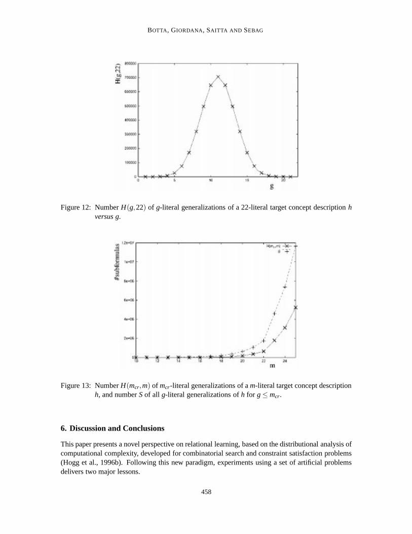
Let m andg denote the number of literals ofh andgenc, respectively. The number ofg-literalgeneralizations ofh, denotedH(g,m), has been analytically computed (see Appendix A). As ex-pected,H(g,m) reaches its maximum forg = m

2 . Figure 12 reportsH(g,m) versusg, for m= 22.

From Figure 13 one can see that the number of generalizations starts growing very fast asmincreases, and that half of them belong to the PT region whenm is greater than twice the criticalvaluemcr.

Both considerations explain why relational learning is more likely to succeed when the sizemof the target concept increasesand is at least twice as great as the critical valuemcr.

457


Figure 12: NumberH(g,22) of g-literal generalizations of a 22-literal target concept descriptionhversus g.

Figure 13: NumberH(mcr,m) of mcr-literal generalizations of am-literal target concept descriptionh, and numberSof all g-literal generalizations ofh for g≤ mcr.

6. Discussion and Conclusions

This paper presents a novel perspective on relational learning, based on the distributional analysis ofcomputational complexity, developed for combinatorial search and constraint satisfaction problems(Hogg et al., 1996b). Following this new paradigm, experiments using a set of artificial problemsdelivers two major lessons.

458


The first lesson concerns the existence of an attractor for relational learning, namely the PTregion. This behavior is not specific to artificial learning problems; it also occurs in real-worldproblems (King et al., 1995; Giordana et al., 1993), as reported by Giordana and Saitta (2000). Thisbehavior is observed for top-down and GA-based search strategies; it is explained by the commonlearning bias toward simplicity (Occam’s Razor), and the fact that discriminating hypotheses mostlylie close to the phase transition.

As the PT region concentrates the (empirically) most complex problem instances, it follows thatrelational learning cannot sidestep the complexity barrier. How to scale up current algorithms (e.g.,in order to learn concepts with more than four variables) thus becomes an open question. Indeed, themost complex applications of relational learning that are described in the literature refer to conceptswith few literals and few variables (King et al., 1995; Giordana et al., 1993; Dolsak et al., 1998).

The second lesson concerns the existence of a “blind spot” for all relational learners consideredin the present study. Whatever the learning problem in this area, the hypotheses extracted from thetraining set behave as random guesses on the test set. This blind spot adversely affects the scalabilityof relational learning, too.

Actually, both results are explained by the same causes, related to the average number of mod-els, associated to a pair (hypothesis, example), and its variance. More precisely, this number ofmodels is high for small-size hypotheses; the existing search criteria (e.g., information gain or min-imum description length) turn out to mislead the search due to the high variance of this number.Meanwhile, the structure of the substitution tree explains both the high computational cost in thePT region, and the fact that discriminating hypotheses belong to it. Of course, the presence of noisyexamples in the training set, and/or irrelevant predicates in the description of the examples, wouldonly make things worse.

These results are worrying, as they suggest that current techniques cannot easily scale up andacquire concepts more complex than those described in the current literature. Meanwhile, the needfor relational learning gets stronger in various large size application domains (e.g., learning fromvisual data; learning from numerical engineering-related data). New approaches should thereforebe devised to address the above limitations.

One perspective for further research concerns the use of bottom-up search strategies for learn-ing concepts in the NO region (that is, for characterizing rare events). The difficulty is twofold.First of all, bottom-up learners are commonly considered less robust than top-down learners (beingsensitive to the order of consideration of the examples on one hand, and to noisy examples on theother hand). Secondly, bottom-up operators such as least general generalization (lgg) or reducedlgg (Nienhuys-Cheng and de Wolf, 1997) are not directly applicable to large size examples. The ar-tificial examples considered in this paper globally contain from 500 to 3,000 tuples (ground literals,in the ILP terminology) in their tables; such sizes are realistic in a numerical engineering context,where meshes involve up to some hundred thousands finite elements.

An alternative might be to exploit any prior knowledge available, and to start the learning searchwith a correct partial hypothesis (informed guess). In this way, the chance of the search beingmisled would be significantly decreased. The limitation is that, even though prior knowledge wouldsignificantly help in finding an accurate solution, the computational complexity of assessing anycandidate hypothesis would remain the same.

A third alternative could be to reconsider the learning strategyand the search criterion. Morespecifically, it would make sense to restrict the exploration to the PT region, given that most relevanthypotheses lie there.

459


Appendix A.

Let c be a target concept whose descriptionh containsm literals, built onmdistinct binary predicatesymbols. The numberH(g,m) of g-literal generalizations ofh with the same number of variablesashis computed according to the following reasoning.

Given the number of variablesn occurring inh, the number of possible variable pairs(Xi,Xj)in a literal of h is K = n2. Any g-literal, n-variable concept description with the same predicatesymbols ash is a subset of byh if and only if all its variables are chained as inh.

Let r j (1≤ j ≤ K) denote the number of literals inh involving a given pair of variables. Byconstruction,

K

∑j=1

r j = m (7)

A g-literal generalization ofh can be obtained by selectingsj literals from ther j ’s (1≤ j ≤K), suchthat∑K

j=1sj = g.Then, the number ofg-literal, n-variable generalizations ofh (up to variable renaming) is given

by:

H(g,m) =K

∑j=1

min(r j ,g−∑ j−1i=1 si)

∑sj=0

(rK

v−∑K−1i=1 si

)K−1

∏i=1

(ri

si). (8)

Let us notice thatH(g,m) is maximum when the numberssi are roughly equal tori2 , that is,g is

aboutm2 .

References

D. Achlioptas, L.M. Kirousis, E. Kranakis, D. Krizanc, and M.S.O. Molloy. Random constraint sat-isfaction: A more accurate picture. InThird International Conference on Principles and Practiceof Constraint Programming, pages 107–120. Springer, 1997.

C. Anglano, A. Giordana, G. Lobello, and L. Saitta. An experimental evaluation of coevolutiveconcept learning. InProceedings of the 15th International Conference on Machine Learning,pages 19–23, Madison, WI, July 1998.

F. Bergadano, A. Giordana, and L. Saitta.Machine Learning: An Integrated Framework and itsApplications. Ellis Horwood, Chichester, UK, 1991.

M. Botta and A. Giordana. SMART+: A multi-strategy learning tool. InIJCAI-93, Proceed-ings of the Thirteenth International Joint Conference on Artificial Intelligence, pages 937–943,Chambery, France, 1993.

M. Botta, A. Giordana, and L. Saitta. An experimental study of phase transitions in matching.In Proceedings of th 16th International Joint Conference on Artificial Intelligence, pages 1198–1203, Stockholm, Sweden, 1999.

M. Botta, A. Giordana, L. Saitta, and M. Sebag. Relational learning: Hard problems and phase tran-sitions. InProceedings of the 6th National Italian Conference on Artificial Intelligence, volumeLNAI 1792, pages 178–189. Springer-Verlag, 2000.

460


P. Cheeseman, B. Kanefsky, and W.M. Taylor. Where the really hard problems are. InProceedings12th International Joint Conference on Artificial Intelligence, pages 331–337, Sidney, Australia,1991.

W. Cohen. A PAC-learning algorithm for a restricted class of recursive logic programs. InProceed-ings 10th National Conference On Artificial Intelligence, Washington, DC, 1993.

J.M. Crawford and L.D Auton. Experimental results on the crossover point in random 3-SAT.Artificial Intelligence, 81:31–58, 1996.

C.J. Date.An Introduction to Database Systems. Addison-Wesley, 1995.

T.G. Dietterich. Approximate statistical tests for comparing supervised classification learning algo-rithms. Neural Computation, 10 (7):1895–1924, 1998.

B. Dolsak, I. Bratko, and A. Jezernik. Application of machine learning in finite element computa-tion. In R.S. Michalski, I. Bratko, and M. Kubat, editors,Machine Learning and Data Mining,pages 147–171. Wiley, 1998.

S. Dzeroski, S. Muggleton, and S. Russell. PAC-learnability of determinate logic programs. InProceedings of COLT-92, pages 128–134, Pittsburgh, PA, 1992.

I.P. Gent and T. Walsh. The TSP phase transition.Artificial Intelligence, 88:349–358, 1996.

A. Giordana and L. Saitta. Phase transitions in relational learning.Machine Learning, 41(2):17–251, 2000.

A. Giordana, L. Saitta, and F. Bergadano. Enigma: A system that learns diagnostic knowledge.IEEE Transactions on Knowledge and Data Engineering, KDE-5:15–28, February 1993.

A. Giordana, L. Saitta, M. Sebag, and M. Botta. Analyzing relational learning in the phase transitionframework. In17th International Conference on Machine Learning, pages 311–318, Stanford,CA, July 2000. Morgan Kaufmann.

T. Hogg, B.A. Huberman, and C.P. Williams, editors.Artificial Intelligence: Special Issue onFrontiers in Problem Solving: Phase Transitions and Complexity, volume 81(1-2). Elsevier,1996a.

T. Hogg, B.A. Huberman, and C.P. Williams. Phase transitions and the search problem.ArtificialIntelligence, 81:1–15, 1996b.

R. Holte, L. Acker, and B. Porter. Concept learning and the problem of small disjuncts. InPro-ceedings of the 11th International Joint Conference on Artificial Intelligence, volume 1, pages813–818, Detroit, MI, 1989. Morgan Kaufmann.

M.J. Kearns and U.V. Vazirani.An Introduction to Computational Learning Theory. MIT Press,1994.

R. Khardon. Learning first order universal Horn expression. InProceedings of COLT-98, pages154–165, Madison, WI, 1998.

461


J.U. Kietz and K. Morik. A polynomial approach to the constructive induction of structural knowl-edge.Machine Learning, 14:193–218, 1994.

R.D. King, A. Srinivasan, and M.J.E. Stenberg. Relating chemical activity to structure: an exami-nation of ILP successes.New Generation Computing, 13:411–433, 1995.

J. Maloberti and M. Sebag. Theta-subsumption in a constraint satisfaction perspective. InProceed-ings of Inductive Logic Programming, pages 164–178. Springer Verlag, LNAI 2157, 2001.

R. Michalski. A theory and methodology of inductive learning. In R. Michalski, J. Carbonell, andT. Mitchell, editors,Machine Learning: An Artificial Intelligence Approach, pages 83–134, LosAltos, CA, 1983. Morgan Kaufmann.

D. Mitchell, B. Selman, and H. Levesque. Hard and easy distributions of SAT problems. In10thNational Conference on Artificial Intelligence, pages 459–465. MIT Press, 1992.

T.M. Mitchell. Generalization as search.Artificial Intelligence, 18:203–226, 1982.

T.M. Mitchell. Machine Learning. McGraw Hill, 1997.

S. Muggleton, editor.Inductive Logic Programming. Academic Press, London, UK, 1992.

S. Muggleton. Inverse entailment and PROGOL.New Gen. Comput., 13:245–286, 1995.

S. Muggleton and L. De Raedt. Inductive logic programming: theory and methods.Journal ofLogic Programming, 19/20:629–679, 1994.

S. Muggleton and C. Feng. Efficient induction of logic programs. In S. Muggleton, editor,InductiveLogic Programming. Academic Press, London, UK, 1992.

S. Nienhuys-Cheng and R. de Wolf.Foundations of Inductive Logic Programming. Springer Verlag,1997.

M.J. Pazzani and D. Kibler. The utility of knowledge in inductive learning.Machine Learning, 9:57–94, 1992.

G. Plotkin. A note on inductive generalization. InMachine Intelligence, volume 5, pages 153–163.Edinburgh University Press, 1970.

P. Prosser. An empirical study of phase transitions in binary constraint satisfaction problems.Arti-ficial Intelligence, 81:81–110, 1996.

R. Quinlan. Learning logical definitions from relations.Machine Learning, 5:239–266, 1990.

R.J. Quinlan. Induction of decision trees.Machine Learning, 1:81–106, 1986.

J. Rissanen. Modeling by shortest data description.Automatica, 14:465–471, 1978.

M. Sebag and C. Rouveirol. Resource-bounded relational reasoning: Induction and deductionthrough stochastic matching.Machine Learning, 38:41–62, 2000.

462


B.M. Smith and M.E. Dyer. Locating the phase transition in binary constraint satisfaction problems.Artificial Intelligence, 81:155–181, 1996.

L.G. Valiant. A theory of the learnable.Communications of the ACM, 27:1134–1142, 1984.

T. Walsh. The constrainedness knife-edge. InProceedings of the 15th National Conference onArtificial Intelligence, pages 406–411, Madison, WI, 1998.

C.P. Williams and T. Hogg. Exploiting the deep structure of constraint problems.Artificial Intelli-gence, 70:73–117, 1994.

463

Documents

Relational Learning as Search in a Critical Regionjmlr.csail.mit.edu/papers/volume4/botta03a/botta03a.pdfJournal of Machine Learning Research 4 (2003) 431-463 Submitted 5/01; Published