Embed Size (px)
Citation preview
Rhode Island CollegeDigital Commons @ RIC
Honors Projects Overview Honors Projects
2019
Relationship Between Financial Markets andNatural Disasters in the USEsteban [email protected]
Follow this and additional works at: https://digitalcommons.ric.edu/honors_projects
Part of the Finance Commons, and the Other Economics Commons
This Honors is brought to you for free and open access by the Honors Projects at Digital Commons @ RIC. It has been accepted for inclusion inHonors Projects Overview by an authorized administrator of Digital Commons @ RIC. For more information, please [email protected].
Recommended CitationGiraldo, Esteban, "Relationship Between Financial Markets and Natural Disasters in the US" (2019). Honors Projects Overview. 154.https://digitalcommons.ric.edu/honors_projects/154
Relationship Between Financial Markets and Natural Disasters in the US
By
Esteban Giraldo
An Honors Project Submitted in Partial Fulfillment
of the Requirements for Honors in the
Department of Economics and Finance
Rhode Island College
2019
TABLE OF CONTENTS
ABSTRACT…………………………………………………………2
INTRODUCTION…………………………………………………...3
LITERATURE REVIEW……………………………………………5
THEORY / HYPOTHESIS………………………………………….9
DATA……………………………………………………………….10
DESCRIPTIVE STATISTICS………………………………………13
EMPIRICAL METHOD…………………………………………....14
EMPIRICAL RESULTS…………………………………………....15
CONCLUSIONS…………………………………………………...17
FUTURE RESEARCH…………………………………………….19
TABLES….…………………………………………………………21
REFERENCES……………………………………………………..41
APPENDIX WEBSITES WHERE DATA WAS COLLECTED.......43
ACKNOWLEDGEMENTS
First, I would like to express my most sincere gratitude to Dr. Kemal Saatcioglu, for his extensive
efforts in helping me complete this project. Similarly, I would like to give a special thanks to Dr.
Sanae Tashiro, who got me started in the process for this project. I would also like to extend a
thank you to the members of the Economics and Finance Departmental Honors Committee,
including: Dr. Kazemi, Dr. Aydogdu, Dr. Blais, and Dr. Basu, for their time and input during the
presentations, as well as the notes I received to improve this paper. Also, I would like to thank the
Economics and Finance Department Chair, Dr. Karim. Everyone’s involvement is highly
appreciated, and this paper reflects the contributions from those mentioned.

2
ABSTRACT
The objective of this study is to find out how different sectors of the market, as defined by the
Bloomberg Industry Classification Standard (BICS), react before and after different natural
disasters, such as hurricanes, earthquakes and tornados. Public cross sectional and time series data
from NOAA, Unisys Weather, and the USGS were collected, in order to build a data set that could
be used for this study. OLS regressions, as well as fixed effects regressions were used to achieve
the results. Among the major findings is a highly significant upward reaction in the returns of the
energy sector when property damage from a tornado occurs.
3
INTRODUCTION
Do stock prices get affected by natural disasters? This is a question that has recently
started to be studied more in academic literature, but one that still needs further exploration since
it could have important trading implications as natural disasters –hurricanes, tornados, and
earthquakes– are natural phenomena that occur on a repeated basis. Does the overall financial
market proxied by S&P 500 or the Dow Jones Industrial Average get affected uniformly or do
different sectors within the financial markets such as financials, materials, utilities, technology,
health care, energy, consumer staples, and consumer discretionary show different reactions to
such events? While several studies to date have looked at the overall financial market reaction to
disasters, this study, to our knowledge, is the first to conduct a systematic analysis of the reaction
of all available individual sectors to natural disasters and attempts to find whether a long, short,
or a combination strategy generates positive returns.
The goal of this study is to come up with a model, or at the very least some rules to use
in case of natural disasters, to mitigate financial losses for individuals. The study uses historical
sector price data of the week an event occurs to assess the price reaction to the event. It further
uses historical sector price data over a longer term to see what type of price trends occur after the
natural disaster. If there are observable price trends for the overall market or for some sectors
within the market, perhaps they can be turned into trading strategies that will yield positive
4
returns. These strategies could then be used by individuals that live in natural disaster-prone
areas and thus are susceptible to losses in the case of natural disasters as well as companies such
as insurers, that would be adversely affected by natural disasters as financial tools that would
help them hedge their exposure to natural disasters.
Major objectives of this project were to come up with a working model using a dataset
that includes weekly returns by sector, compared to different natural disasters occurring per week
and hopefully coming up with the effect of said natural disasters on returns. This paper collects
twenty-eight years of weekly returns in the different sectors of the market, as well as data of
twenty-eight years of hurricanes per week, and earthquakes per week. Along with tornados per
week, the damage attributed to each tornado is also collected. All the data is for disasters that
happened on the continental United States. Recently researchers have started paying attention to
this topic especially since the occurrence of natural disasters has increased as climate change
takes effect on our world. For example, Koerniadi, et. al. (2012) find evidence suggesting
earthquakes, hurricanes and tornados could negatively affect market returns several weeks after
the events, while other disasters such as flood, tsunami and volcanic eruption may have limited
impact on market returns.
The major contribution of this paper to the existing literature is a detailed look at
twenty-eight years of weekly disaster data and its effect on stock markets not only in the
5
aggregate but also on a sector basis. This paper’s major findings include a confirmation of a
negative effect on the cumulative stock market, when a catastrophe has occurred with high
statistical significance. Furthermore, it confirms that returns for the market as whole go down
when Property Damage from a tornado occurs. But when broken down by sector, this same
Property Damage has a positive effect on the returns of the energy sector, and it is highly
statistically significant. Other significant findings when broken down by sector are, that the
returns of the DOW Jones Industrial Average and the Industrial sector are both affected
negatively when a catastrophe transpires.
LITERATURE REVIEW
Several studies show there is a correlation between asset prices and natural disasters. [Barro
(2009), Koerniadi, et. al. (2012), Nakamura (2013), Seetharam (2017)] They investigate the
extent of the decline before and immediately after a disaster, and the length of time a recovery
takes to develop. This paper builds on their work in setting the parameters for the dataset and
their analysis.
Barro (2009), Koerniadi, et. al. (2012), and Nakamura (2013) focus on large scale disasters
such as World Wars and Pandemics. They attempt to come up with a risk premium in order to
make up for the potential loss during these great disasters. Nakamura (2013) finds a rather large
value for their risk premium and reports: “Our model generates a sizable equity premium from
6
disaster risk, but one that is substantially smaller than in simpler models. It implies that a large
value of the intertemporal elasticity of substitution is necessary to explain stock-market crashes
at the onset of disasters.” [Nakamura (2013)]. The data for this study comes from an annual
consumption dataset created by Barro and Ursua (2008) which includes 100 years of data from
24 different countries. Nakamura (2013) uses the Markov-Chain Monte-Carlo (MCMC) methods
to conduct the empirical analysis. The goal of the study was to judge the size of the shocks
during a disaster period, as well as the extent of recovery after disasters. Although this study
focuses on disasters that from peak to trough last about 6 years; it also tests if a disaster started
and ended immediately. The findings are that equities fare extremely poorly relative to bonds at
times of a disaster, and this behavior generates a large equity premium in normal times.
[Nakamura (2013)]. This disaster effect coincides with the hypothesis of this paper that natural
disasters will have a negative effect on stock returns. In comparison to these long-term disasters,
however, weather catastrophes occur and end pretty much as soon as they begin.
In his “Rare Disasters, Asset Prices, and Welfare Costs” article published in the American
Economic Review, Barro (2009) builds on his previous work with a data set that considers 60
events for 35 countries over 100 years. It adds more parameters to account for asset pricing in
different economies. This study also focuses on large economic disasters; but Barro notes: “In
contrast, the probability parameter p and size parameter b refer to major economic disasters,
7
such as those that occurred in many countries during World Wars I and II and the Great
Depression. … To go further, decreases in p or b constitute reductions in the probability or size
of disasters not yet seen or, at least, not seen in the 20th century. Included here would be nuclear
conflicts, large scale natural disasters (tsunamis, hurricanes, earthquakes, asteroid collisions),
and epidemics of disease (Black Death, avian flu).” [Barro (2009)]. When we apply these results
to weather related disasters, we can conclude that the welfare costs of disaster risk will lower
GDP, therefore the perception of a disaster can create the fear that the stock market will drop
because of the forward-looking decline in aggregate consumption, making the analysis in this
paper relevant.
In “Natural disasters – Blessings in disguise?” Koerniadi, et. al. (2012) examine the impact
of natural disasters on market returns and on several industries. The authors indicate the reason
for their study as the prediction by Oxford University researchers that natural disasters will
increase in the coming decade due to global warming. The study includes earthquakes,
hurricanes, tornados, floods, tsunamis, and volcanic eruptions, that occurred in numerous
countries with developed stock markets. They study how these events affect market returns and
the returns of several industries, expected to be most affected in a negative or positive manner.
They find that natural disasters do in fact have a negative effect on certain sectors and industries.
The setup of Koerniadi, et. al. (2012) is the most similar to this research paper. Where they differ
8
is that the focus of this study is only on US based catastrophes and markets, and Koerniadi, et. al.
(2012) does not include macroeconomic control variables, such as CPI or GDP. They do find that
market returns react negatively to earthquakes, hurricanes and tornados which is in line with the
questions and expectations of this paper.
Seetharam (2017) describes the impact of 122 major catastrophic events, on publicly listed
companies that were geographically affected by these events. The study compares the returns of
exposed companies to non-exposed companies, using a standard cross-sectional event study
methodology. Another question Seetharam (2017) attempts to answer is whether the impact to
exposed companies is worse on multi-plant firms vs. single-plant firms. The findings include:
“The estimates suggest a sizable decline in the value of exposed firms relative to nonexposed
firms. The immediate effect … is small and only significant at the 10% level, but the effect in
longer horizons are all larger and significant at the 1% level.” The study estimates the fall in
market valuation to be 0.3 and 0.7 percentage points in the 15-day horizon and the 45-day
horizon, respectively. The adverse impact is found to be mainly centered on single-plant
standalone firms and multi-plant firms seem to retain their adaptive capacity to counter the
adverse costs of extreme weather. The results of this study are very relevant to this study because
it has similar findings of negative effects from catastrophes on market returns or company
9
valuations while using a cross-sectional event study methodology as opposed to the fixed effects
OLS method used here.
THEORY AND TESTABLE HYPOTHESIS
The theory in this paper is that when natural disasters occur, there will be a measurable
negative effect on weekly returns in most sectors and market indices. The findings here are
similar to those in Koerniadi, et. al. (2012): “We find that different natural disasters have
different impacts on the returns of the market and on those of industries. Our evidence suggests
that while earthquake, hurricane and tornado could negatively affect market returns several
weeks after the events, other disasters such as flood, tsunami and volcanic eruption may have
limited impact on market returns”. Furthermore, these disasters could potentially have a positive
effect on other sectors.
Unlike Koerniadi, et. al. (2012) the data for this study is controlled for inflation,
unemployment, GDP, the purchasing managers index, and mortgage applications, to help show
the isolated effects on returns caused by catastrophes and property damage. This paper
hypothesizes that, if a natural disaster occurs, there will be a quantifiable effect on weekly
returns.
Hypothesis Independent Variable
β Expected Sign
Theory/Existing Findings
H1 Returns β1 β1 < 0 Natural disasters will have a negative effect on weekly financial market returns (Y).
10
DATA
This paper uses financial and economic data obtained from the Bloomberg terminals in the
Rhode Island College Finance Lab. It contains twenty-eight years of weekly price data starting in
January 1990 and going through April 2018, for the overall market indices Dow Jones Industrial
Average (DJIA), Standard & Poor’s 500 (S&P 500), Nasdaq Composite, and Russell 2000, as
well as the following nine sectors: Materials, Industrials, Technology, Health Care, Consumer
Staples, Consumer Discretionary, Energy, Financials, Utilities. Once this data was collected the
price information was used to calculate the returns per week for the 28 years of data which left
1,456 observations for each sector and market index, or 18,928 total return observations.
Hurricane data was taken from the Unisys Weather website1. The data was broken down by
week and category for each hurricane that occurred in the past twenty-eight years were provided.
The earthquake data was found on the United States Geological Survey (USGS) website2 where
it was listed by date. The tornado information along with the property damage data contained in
this paper was acquired from the National Oceanic and Atmospheric Administration (NOAA)
website3. Dummy variables were used to designate if there was an event that week (1) or not (0).
1 https://www.unisys.com/industries/government/unisys-federal/unisys-weather 2 https://pubs.usgs.gov/gip/earthq4/severitygip.html 3 https://www.nssl.noaa.gov/education/svrwx101/tornadoes/
11
The data for natural disasters was collected starting with tornados greater than EF-3 on the
Enhanced Fujita Scale4, which includes tornados with wind speeds of 136 mph or higher. EF-3
damage is considered severe, and roofs, heavy cars, trees and structures with weak foundations
will be blown away some distance with the damage increasing with each category up to EF-5
where winds exceed 200 mph. The property damage in millions of dollars accredited to each
tornado was also recorded when this value was higher than $2.5 million. Moving onto
hurricanes, data for those greater than category 3 were collected. These hurricanes have wind
speeds higher than 111 mph. According to the Saffir-Simpson Hurricane Wind Scale which is
used by NOAA, “hurricanes reaching category 3 or higher are considered major hurricanes
because of their potential for significant loss of life and damage.5” Finally, earthquakes greater
than 4 on the Richter scale were added to the data set. According to the USGS, earthquakes of
magnitude 4 and higher are felt by people and some damage can occur.
The economic data collected from the Bloomberg terminal were the top-rated market
indicators by analysts in Bloomberg, which were mortgage applications and the Purchasing
Managers Index. Also, the Federal Reserve Economic Data (FRED) website6 was used to collect
twenty-eight years of monthly data for CPI, real GDP, and the Unemployment Rate. These
4 https://weather.com/storms/tornado/news/enhanced-fujita-scale-20130206 5 https://www.nhc.noaa.gov/aboutsshws.php 6 https://fred.stlouisfed.org
12
macroeconomic indicators were selected due to the extensive research that shows these
fundamental variables to have power in predicting stock returns. Chen, Roll and Ross (1986) find
that changes in aggregate production, inflation, and the short-term interest rates are among the
macroeconomic factors that have some power to predict stock returns and they conclude that
expected returns are a function of business conditions. The unemployment rate, also followed
closely by the federal reserve, was selected as a barometer of economic activity proxying for the
health of the current economy.
In total the dataset contains 29,120 different datapoints which are observations of the
same entities per week, year over year, for twenty-eight years. This makes it a cross-sectional
panel-data, so regression methods were adjusted as such. The dependent variables used in the
empirical model are the returns of the indexes and the sectors used (Y). After some data analysis,
the individual dummy variables of Hurricanes, Tornados and Earthquakes were found not to be
statistically significant on their own. Subsequently, they were combined to create a consolidated
variable called Catastrophe which did show statistical significance when it came to predicting
market returns. The independent variables used in the study include this new Catastrophe dummy
variable ranging from 0 to 3 (X1), Consumer Price Index or CPI (X2), Unemployment Rate (X3),
Gross Domestic Product or GDP (X4), Purchasing Managers Index or PMI (X5), Mortgage
13
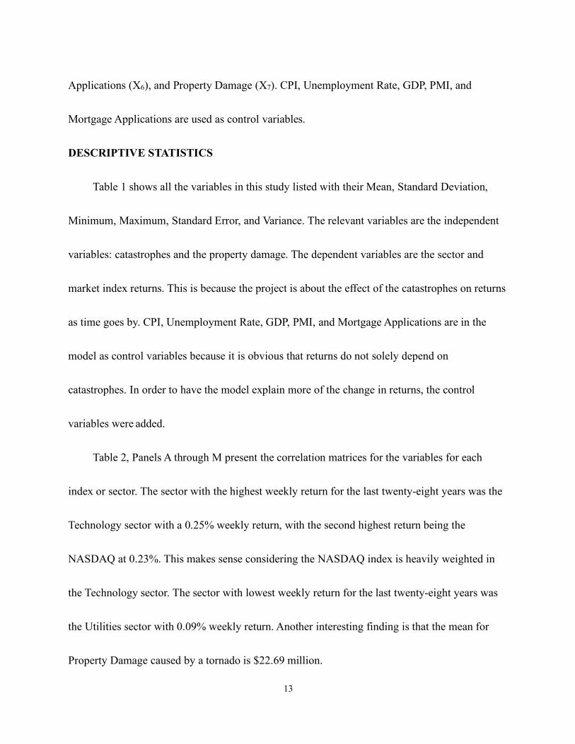
Applications (X6), and Property Damage (X7). CPI, Unemployment Rate, GDP, PMI, and
Mortgage Applications are used as control variables.
DESCRIPTIVE STATISTICS
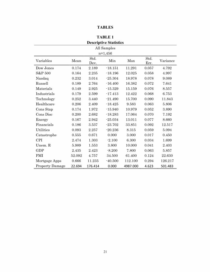
Table 1 shows all the variables in this study listed with their Mean, Standard Deviation,
Minimum, Maximum, Standard Error, and Variance. The relevant variables are the independent
variables: catastrophes and the property damage. The dependent variables are the sector and
market index returns. This is because the project is about the effect of the catastrophes on returns
as time goes by. CPI, Unemployment Rate, GDP, PMI, and Mortgage Applications are in the
model as control variables because it is obvious that returns do not solely depend on
catastrophes. In order to have the model explain more of the change in returns, the control
variables were added.
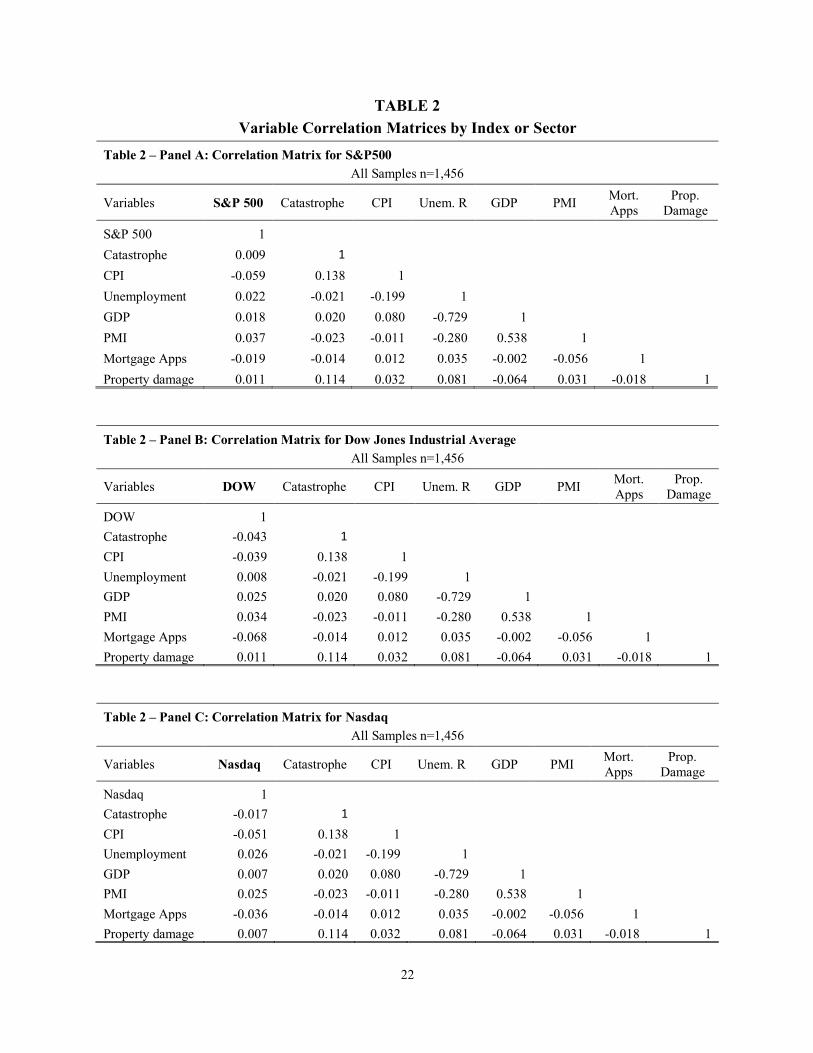
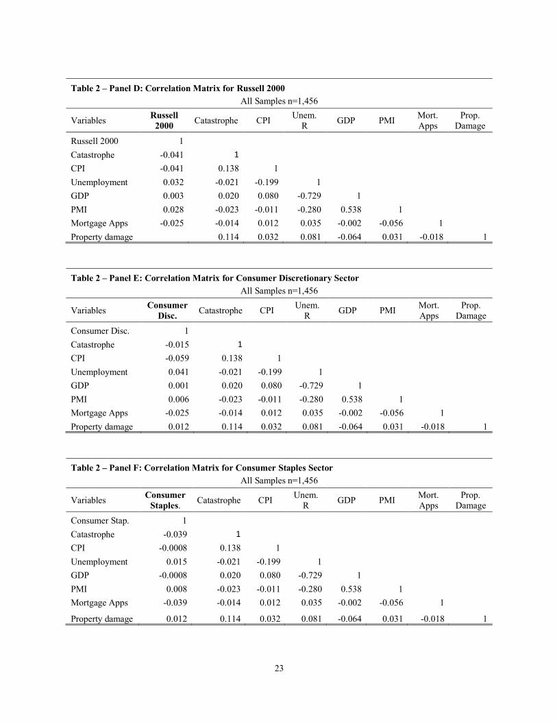
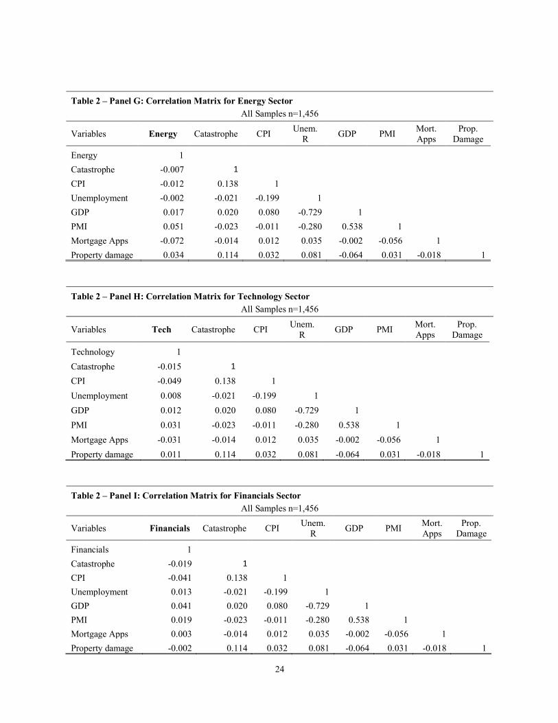
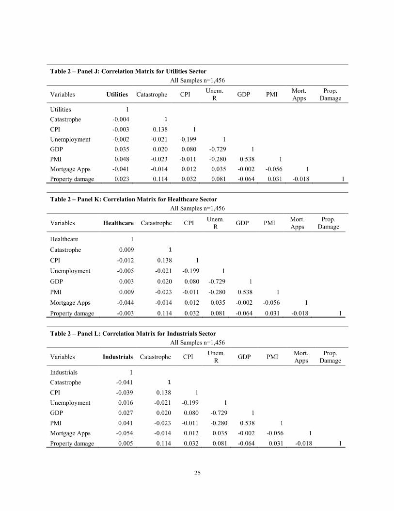
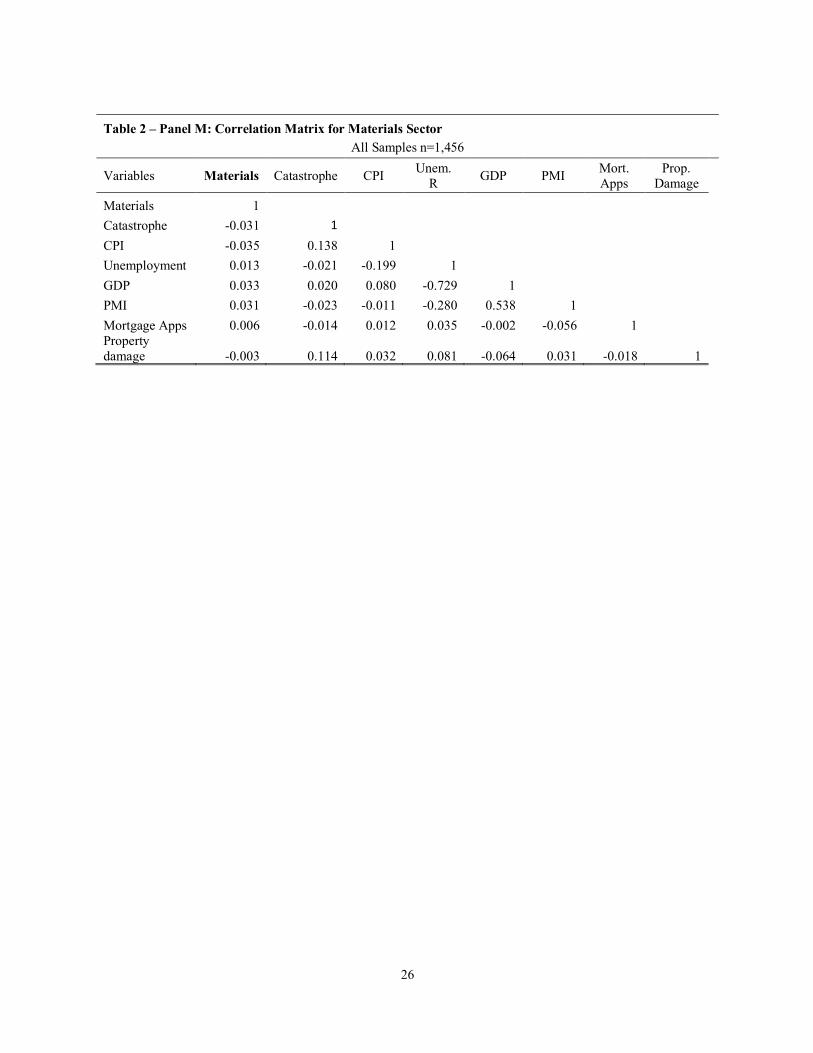
Table 2, Panels A through M present the correlation matrices for the variables for each
index or sector. The sector with the highest weekly return for the last twenty-eight years was the
Technology sector with a 0.25% weekly return, with the second highest return being the
NASDAQ at 0.23%. This makes sense considering the NASDAQ index is heavily weighted in
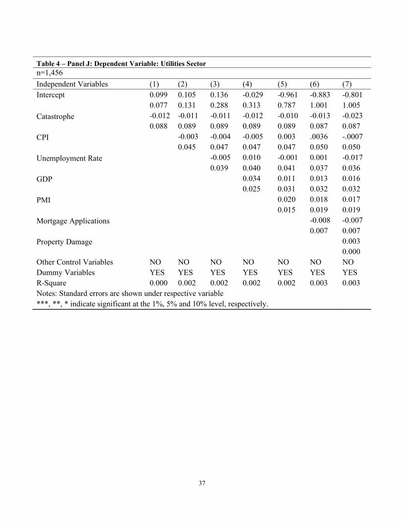
the Technology sector. The sector with lowest weekly return for the last twenty-eight years was
the Utilities sector with 0.09% weekly return. Another interesting finding is that the mean for
Property Damage caused by a tornado is $22.69 million.
14
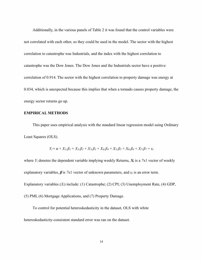
Additionally, in the various panels of Table 2 it was found that the control variables were
not correlated with each other, so they could be used in the model. The sector with the highest
correlation to catastrophe was Industrials, and the index with the highest correlation to
catastrophe was the Dow Jones. The Dow Jones and the Industrials sector have a positive
correlation of 0.914. The sector with the highest correlation to property damage was energy at
0.034, which is unexpected because this implies that when a tornado causes property damage, the
energy sector returns go up.
EMPIRICAL METHODS
This paper uses empirical analysis with the standard linear regression model using Ordinary
Least Squares (OLS).
Yi = α + X1i β1 + X2i β2 + X3i β3 + X4i β4 + X5i β5 + X6i β6 + X7i β7 + εi
where Yi denotes the dependent variable implying weekly Returns, Xi is a 7x1 vector of weekly
explanatory variables, β is 7x1 vector of unknown parameters, and εi is an error term.
Explanatory variables (Xi) include: (1) Catastrophe; (2) CPI; (3) Unemployment Rate, (4) GDP,
(5) PMI, (6) Mortgage Applications, and (7) Property Damage.
To control for potential heteroskedasticity in the dataset, OLS with white
heteroskedasticity-consistent standard error was ran on the dataset.
15
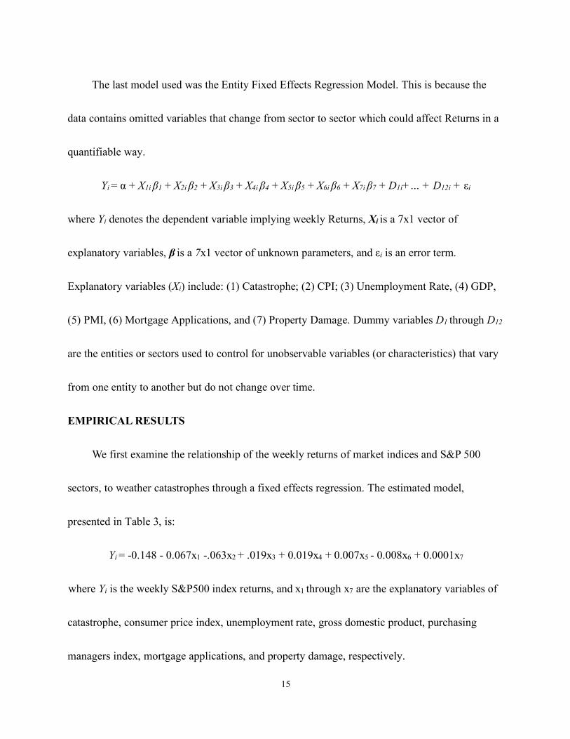
The last model used was the Entity Fixed Effects Regression Model. This is because the
data contains omitted variables that change from sector to sector which could affect Returns in a
quantifiable way.
Yi = α + X1i β1 + X2i β2 + X3i β3 + X4i β4 + X5i β5 + X6i β6 + X7i β7 + D1i+… + D12i + εi
where Yi denotes the dependent variable implying weekly Returns, Xi is a 7x1 vector of
explanatory variables, β is a 7x1 vector of unknown parameters, and εi is an error term.
Explanatory variables (Xi) include: (1) Catastrophe; (2) CPI; (3) Unemployment Rate, (4) GDP,
(5) PMI, (6) Mortgage Applications, and (7) Property Damage. Dummy variables D1 through D12
are the entities or sectors used to control for unobservable variables (or characteristics) that vary
from one entity to another but do not change over time.
EMPIRICAL RESULTS
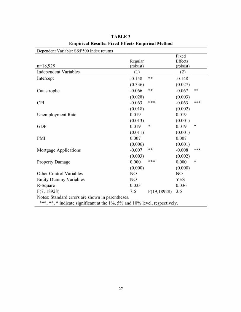
We first examine the relationship of the weekly returns of market indices and S&P 500
sectors, to weather catastrophes through a fixed effects regression. The estimated model,
presented in Table 3, is:
Yi = -0.148 - 0.067x1 -.063x2 + .019x3 + 0.019x4 + 0.007x5 - 0.008x6 + 0.0001x7
where Yi is the weekly S&P500 index returns, and x1 through x7 are the explanatory variables of
catastrophe, consumer price index, unemployment rate, gross domestic product, purchasing
managers index, mortgage applications, and property damage, respectively.
16
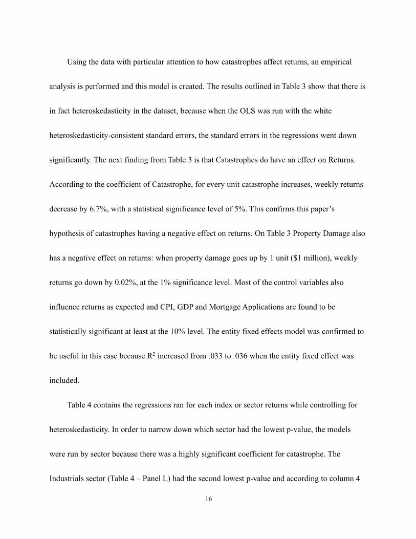
Using the data with particular attention to how catastrophes affect returns, an empirical
analysis is performed and this model is created. The results outlined in Table 3 show that there is
in fact heteroskedasticity in the dataset, because when the OLS was run with the white
heteroskedasticity-consistent standard errors, the standard errors in the regressions went down
significantly. The next finding from Table 3 is that Catastrophes do have an effect on Returns.
According to the coefficient of Catastrophe, for every unit catastrophe increases, weekly returns
decrease by 6.7%, with a statistical significance level of 5%. This confirms this paper’s
hypothesis of catastrophes having a negative effect on returns. On Table 3 Property Damage also
has a negative effect on returns: when property damage goes up by 1 unit ($1 million), weekly
returns go down by 0.02%, at the 1% significance level. Most of the control variables also
influence returns as expected and CPI, GDP and Mortgage Applications are found to be
statistically significant at least at the 10% level. The entity fixed effects model was confirmed to
be useful in this case because R2 increased from .033 to .036 when the entity fixed effect was
included.
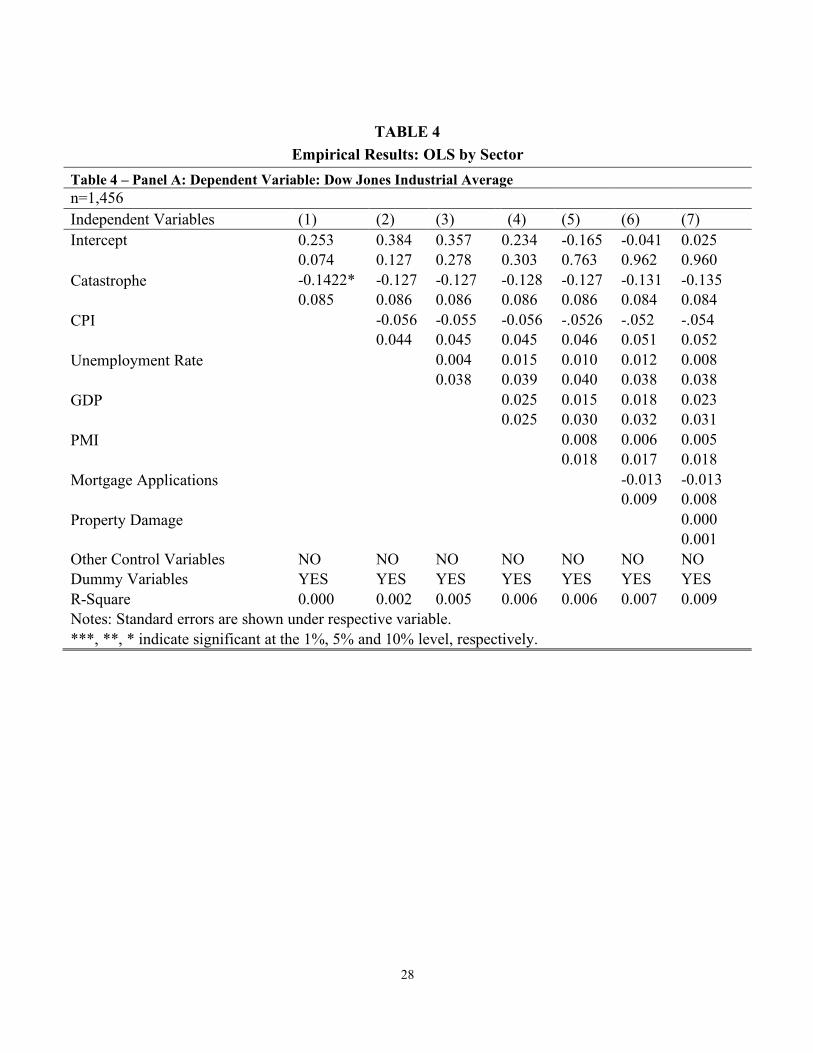
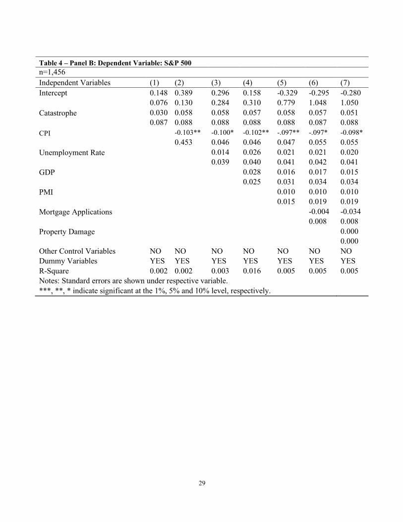
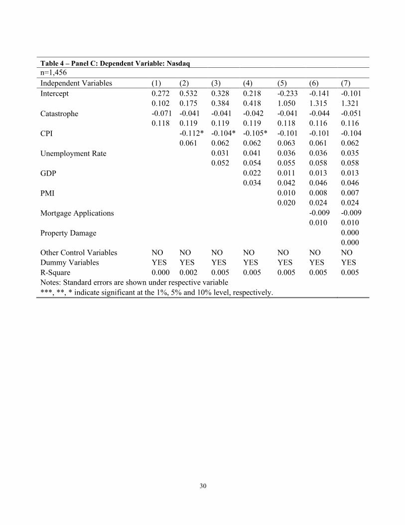
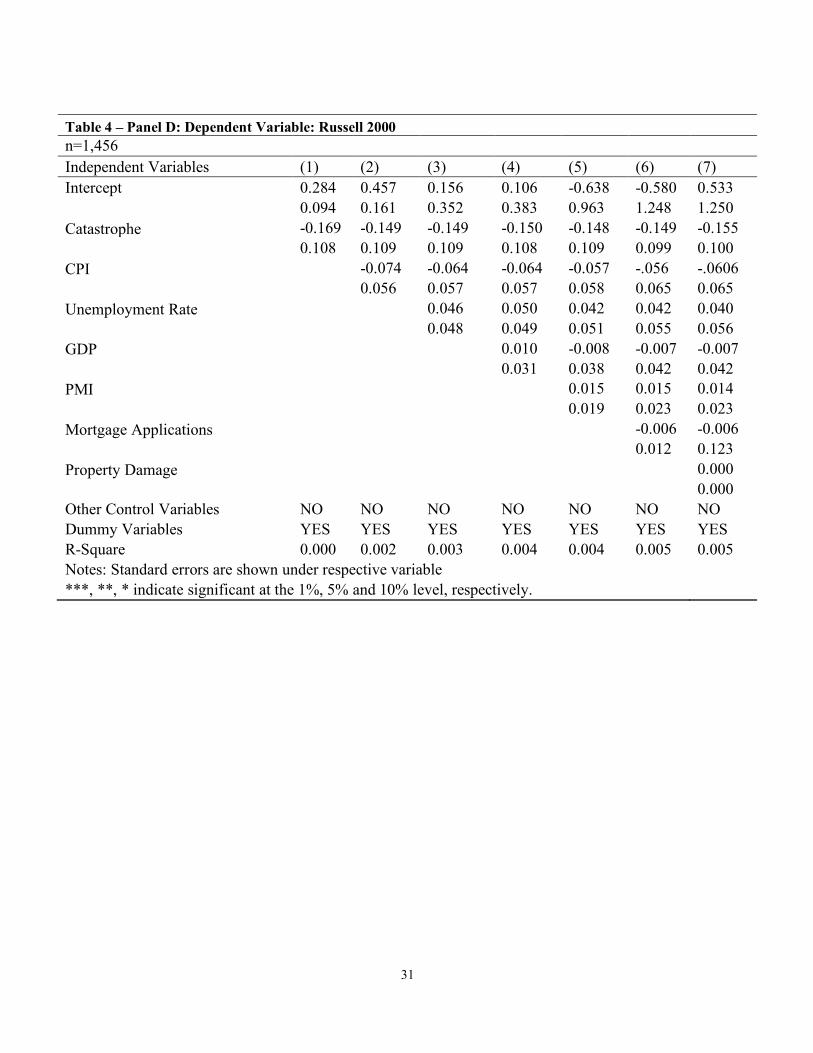
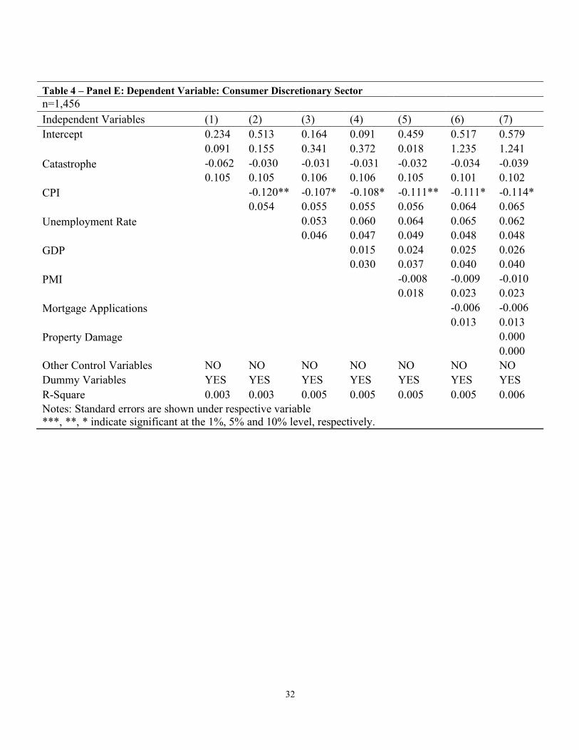
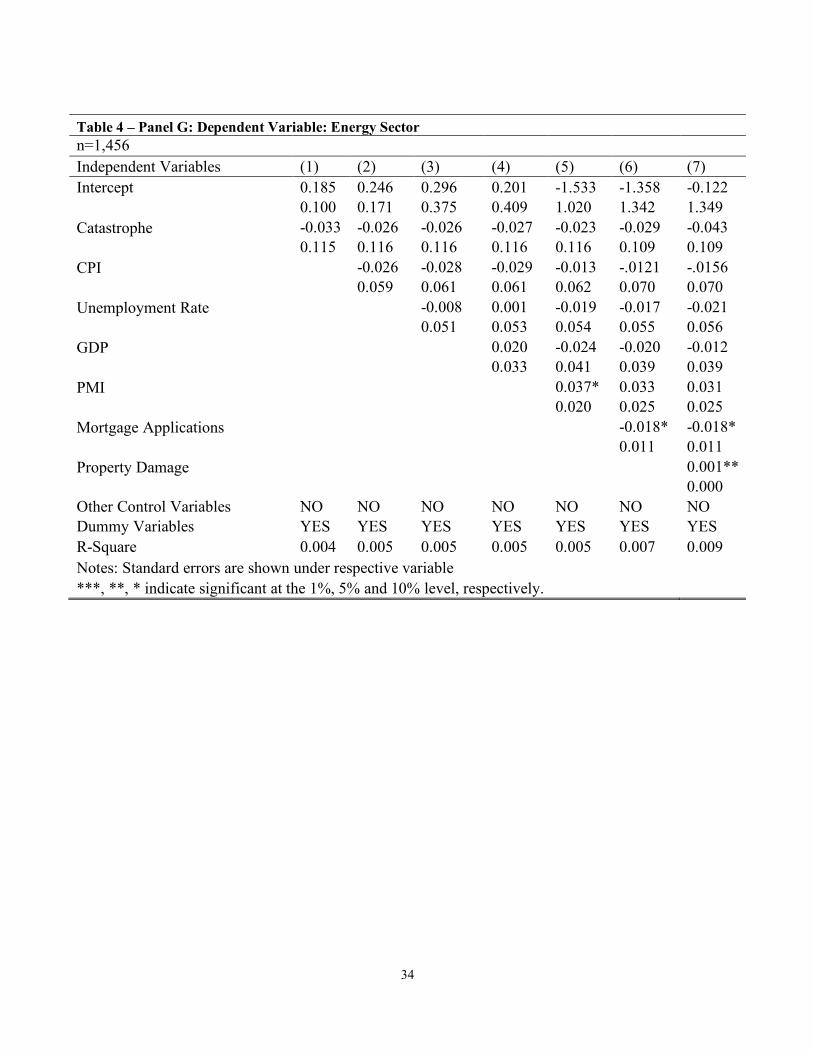
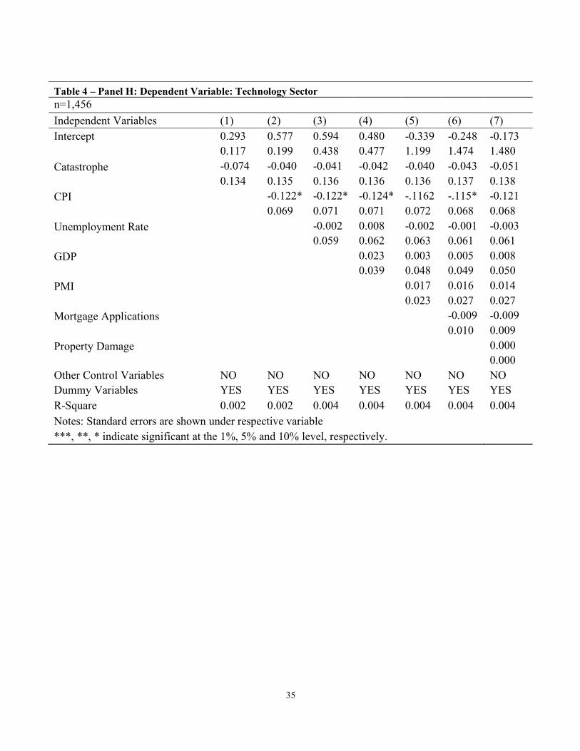
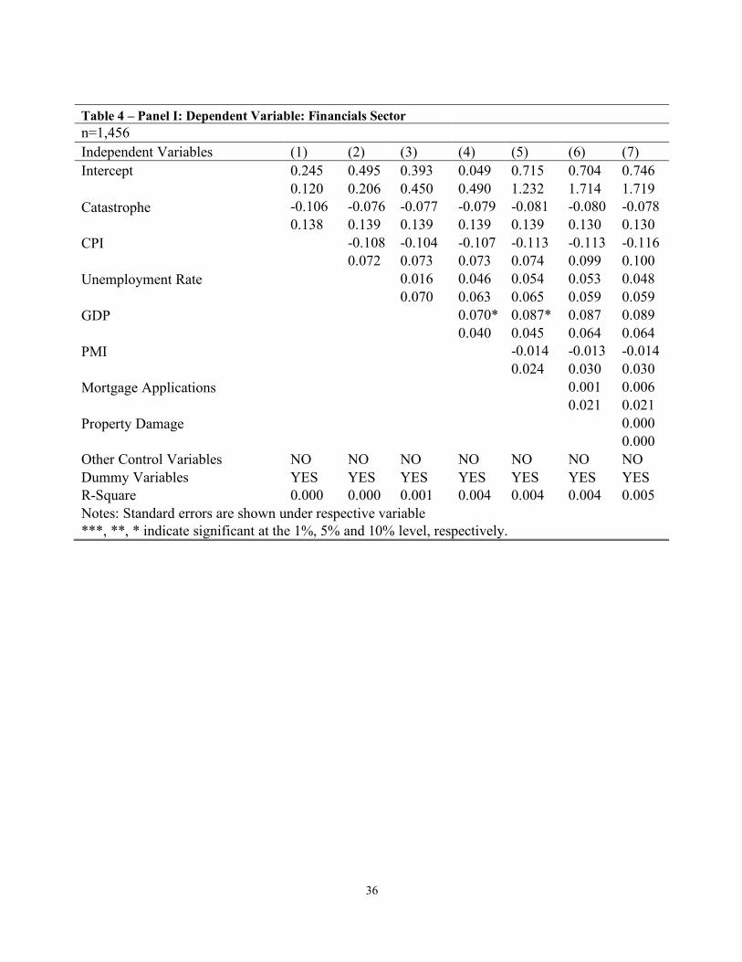
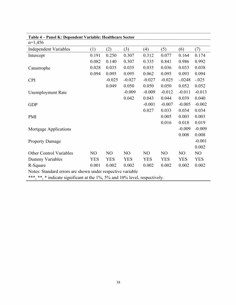
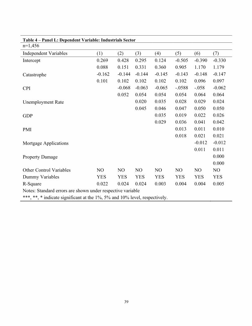
Table 4 contains the regressions ran for each index or sector returns while controlling for
heteroskedasticity. In order to narrow down which sector had the lowest p-value, the models
were run by sector because there was a highly significant coefficient for catastrophe. The
Industrials sector (Table 4 – Panel L) had the second lowest p-value and according to column 4
17
the returns go down by 1.4% every time catastrophe increases by 1 unit, at a statistical
significance level of 15%. Industrials also had the highest negative correlation with catastrophe
out of all the other sectors. The p-value for the Dow Jones (Table 4 – Panel A) was even lower
just above the 10% level of significance at 0.105.
One more interesting discovery is that the variable Property Damage has highly significant
results for the energy sector on Table 4 – Panel G. For every unit that Property Damage goes up,
energy sector returns go up by .01%, at the 5% level of significance. These findings are very
exciting because they offer a clue on which way to continue this research. Diaz de Gracia (2016)
investigate the impact of oil prices on stock returns from January 1974 to December 2015 and
find that in the short run a significant positive impact to oil prices is beneficial to energy stock
prices. They also find that this relationship becomes statistically significant after 1986. [Liu, et.
al. (2017)]. This could explain why the Energy sector returns increase when there is property
damage from a tornado, because when infrastructure and pipelines are damaged this can cause a
contraction in the oil supply which in the short term leads to an increase in the price of oil and
therefore, leading to an increase in Energy sector prices. We leave investigating the long-term
effects of this on Energy sector prices to a future study.
18
CONCLUSIONS AND DISCUSSION
When large scale external shocks occur, stock markets are expected to be affected in
different ways depending on the index or industry. The worse the disaster (and the more
unexpected it is) the higher the stock market reaction is expected to be. This study finds that
there is in fact a negative relationship between catastrophes and returns, with high statistical
significance which is consistent with the literature that has been compiled by academia.
According to the findings, when a catastrophe happens, returns go down but historically not by
much. This can be attributed to the sheer size of the financial markets, especially in the US
where NYSE alone trades at a daily volume of $169 billion. “The costliest natural catastrophe
recorded to date is the 2005 landfall of Hurricane Katrina in Louisiana, with an estimated
destructive cost of around $150 billion, of which $62 billion was covered by the insurance
industry. This is less than a single percentage point of movement on the New York Stock
Exchange.” [Mahalingam, et. al. (2018)]. As the global economy becomes more intertwined, and
weather disasters become more destructive, we would expect the costs to keep increasing making
the negative effects greater on financial markets as time goes on.
Market indices and Industries were also tested against catastrophes, and the Dow Jones and
Industrials sector had the highest statistical significance in this test at 15% and 10.5%,
respectively. One explanation for this is that when catastrophes ensue, the destruction of property
19
take its toll on these industries, such as Airlines, Air freight, Road and Rail, and Transportation
Infrastructure. The price of oil can be pushed up when a catastrophe transpires, which directly
hurts the industries just mentioned because it makes their cost to operate more expensive. This
cost increase compiled with the capital investment necessary to fix whatever broke after a
catastrophe, can drive investors to sell off the Industrials as soon as bad weather hits. Since the
Dow Jones is heavily weighted with Industrials, and since it has a very high correlation with it,
these effects show up in both asset classes.
The highest statistical significance of the explanatory variables to any sector is the positive
relationship between the Property Damage variable to the energy sector. “The oil and gas
industry has been favoured by investors in recent years due to the increasing oil prices during
the period between 2008 and 2014. The number of mutual funds and exchange traded funds that
invest in oil and gas industry companies also increased during this period.” [Ramos and Veiga
(2011)]. This positive relationship between oil prices and asset prices explains the positive
coefficient generated for property damage. A more counterintuitive argument is that due to the
destruction of property, capital investments will follow, some paid for by insurances. This would
lead to upgraded infrastructure at a lower cost than if they paid for it without the insurance
payout.
20
FUTURE RESEARCH
Future research should include more controlled variables, and new variables like P/E ratios,
Return on Equity, Risk free rate, 10-year T-bill rate, WTI Oil price and the Price to dividend
ratio. This would be important in order to continue to increase the R-squared for this model.
Expanding this research can lead to a pathway for investing during different types of events that
are unexpected and affect returns.
The next step to further this research would be to perform an event study as in Ruiz, et. al.
(2014). “These studies are useful because the event’s effect is immediately reflected in stock
prices (Fama, et al., 1969). Therefore, a measure of the economic impact of the event can be
easily developed using the observed prices of securities over a short period of time.” [Ruiz, et.
al. (2014)]. There could be several event studies performed, one using the returns of when the
largest Property Damages recorded happen. Another study that can be done is to come up with a
predictions for the timing of catastrophes (for example using time series analysis or even
artificial intelligence or neural networks) and then investigate in the event study the months
when catastrophes are abnormally high or low compared to the predictions, to see if the
contemporaneous or subsequent returns are also abnormally high or low.
21
TABLES
TABLE 1 Descriptive Statistics
All Samples n=1,456
Variables Mean Std. Dev. Min Max Std.
Err. Variance
Dow Jones 0.174 2.189 -18.151 11.291 0.057 4.792 S&P 500 0.164 2.235 -18.196 12.025 0.058 4.997 Nasdaq 0.232 3.014 -25.304 18.978 0.078 9.089 Russell 0.189 2.764 -16.400 16.382 0.072 7.641 Materials 0.149 2.925 -15.329 15.159 0.076 8.557 Industrials 0.179 2.599 -17.413 12.422 0.068 6.753 Technology 0.252 3.440 -21.490 15.700 0.090 11.843 Healthcare 0.206 2.409 -18.425 9.583 0.063 5.806 Cons Stap 0.174 1.972 -15.940 10.979 0.052 3.890 Cons Disc 0.200 2.682 -18.283 17.064 0.070 7.192 Energy 0.167 2.942 -25.034 13.011 0.077 8.660 Financials 0.186 3.537 -23.702 33.851 0.092 12.517 Utilities 0.093 2.257 -20.236 8.315 0.059 5.094 Catastrophe 0.555 0.671 0.000 3.000 0.017 0.450 CPI 2.474 1.303 -2.100 6.300 0.034 1.699 Unem. R 5.989 1.553 3.800 10.000 0.041 2.403 GDP 2.435 2.423 -8.200 7.800 0.063 5.857 PMI 52.092 4.757 34.500 61.400 0.124 22.630 Mortgage Apps 0.666 11.235 -40.500 112.100 0.294 126.217 Property Damage 22.694 176.414 0.000 4987.000 4.623 501.483
22
TABLE 2 Variable Correlation Matrices by Index or Sector
Table 2 – Panel A: Correlation Matrix for S&P500 All Samples n=1,456
Variables S&P 500 Catastrophe CPI Unem. R GDP PMI Mort. Apps
Prop. Damage
S&P 500 1 Catastrophe 0.009 1 CPI -0.059 0.138 1 Unemployment 0.022 -0.021 -0.199 1 GDP 0.018 0.020 0.080 -0.729 1 PMI 0.037 -0.023 -0.011 -0.280 0.538 1 Mortgage Apps -0.019 -0.014 0.012 0.035 -0.002 -0.056 1 Property damage 0.011 0.114 0.032 0.081 -0.064 0.031 -0.018 1
Table 2 – Panel B: Correlation Matrix for Dow Jones Industrial Average All Samples n=1,456
Variables DOW Catastrophe CPI Unem. R GDP PMI Mort. Apps
Prop. Damage
DOW 1 Catastrophe -0.043 1 CPI -0.039 0.138 1 Unemployment 0.008 -0.021 -0.199 1 GDP 0.025 0.020 0.080 -0.729 1 PMI 0.034 -0.023 -0.011 -0.280 0.538 1 Mortgage Apps -0.068 -0.014 0.012 0.035 -0.002 -0.056 1 Property damage 0.011 0.114 0.032 0.081 -0.064 0.031 -0.018 1
Table 2 – Panel C: Correlation Matrix for Nasdaq All Samples n=1,456
Variables Nasdaq Catastrophe CPI Unem. R GDP PMI Mort. Apps
Prop. Damage
Nasdaq 1 Catastrophe -0.017 1 CPI -0.051 0.138 1 Unemployment 0.026 -0.021 -0.199 1 GDP 0.007 0.020 0.080 -0.729 1 PMI 0.025 -0.023 -0.011 -0.280 0.538 1 Mortgage Apps -0.036 -0.014 0.012 0.035 -0.002 -0.056 1 Property damage 0.007 0.114 0.032 0.081 -0.064 0.031 -0.018 1
23
Table 2 – Panel D: Correlation Matrix for Russell 2000
All Samples n=1,456
Variables Russell 2000 Catastrophe CPI Unem.
R GDP PMI Mort. Apps
Prop. Damage
Russell 2000 1 Catastrophe -0.041 1 CPI -0.041 0.138 1 Unemployment 0.032 -0.021 -0.199 1 GDP 0.003 0.020 0.080 -0.729 1 PMI 0.028 -0.023 -0.011 -0.280 0.538 1 Mortgage Apps -0.025 -0.014 0.012 0.035 -0.002 -0.056 1 Property damage 0.114 0.032 0.081 -0.064 0.031 -0.018 1
Table 2 – Panel E: Correlation Matrix for Consumer Discretionary Sector All Samples n=1,456
Variables Consumer Disc. Catastrophe CPI Unem.
R GDP PMI Mort. Apps
Prop. Damage
Consumer Disc. 1 Catastrophe -0.015 1 CPI -0.059 0.138 1 Unemployment 0.041 -0.021 -0.199 1 GDP 0.001 0.020 0.080 -0.729 1 PMI 0.006 -0.023 -0.011 -0.280 0.538 1 Mortgage Apps -0.025 -0.014 0.012 0.035 -0.002 -0.056 1 Property damage 0.012 0.114 0.032 0.081 -0.064 0.031 -0.018 1
Table 2 – Panel F: Correlation Matrix for Consumer Staples Sector All Samples n=1,456
Variables Consumer Staples. Catastrophe CPI Unem.
R GDP PMI Mort. Apps
Prop. Damage
Consumer Stap. 1 Catastrophe -0.039 1 CPI -0.0008 0.138 1 Unemployment 0.015 -0.021 -0.199 1 GDP -0.0008 0.020 0.080 -0.729 1 PMI 0.008 -0.023 -0.011 -0.280 0.538 1 Mortgage Apps -0.039 -0.014 0.012 0.035 -0.002 -0.056 1 Property damage 0.012 0.114 0.032 0.081 -0.064 0.031 -0.018 1
24
Table 2 – Panel G: Correlation Matrix for Energy Sector All Samples n=1,456
Variables Energy Catastrophe CPI Unem. R GDP PMI Mort.
Apps Prop.
Damage
Energy 1 Catastrophe -0.007 1 CPI -0.012 0.138 1 Unemployment -0.002 -0.021 -0.199 1 GDP 0.017 0.020 0.080 -0.729 1 PMI 0.051 -0.023 -0.011 -0.280 0.538 1 Mortgage Apps -0.072 -0.014 0.012 0.035 -0.002 -0.056 1 Property damage 0.034 0.114 0.032 0.081 -0.064 0.031 -0.018 1
Table 2 – Panel H: Correlation Matrix for Technology Sector All Samples n=1,456
Variables Tech Catastrophe CPI Unem. R GDP PMI Mort.
Apps Prop.
Damage
Technology 1 Catastrophe -0.015 1 CPI -0.049 0.138 1 Unemployment 0.008 -0.021 -0.199 1 GDP 0.012 0.020 0.080 -0.729 1 PMI 0.031 -0.023 -0.011 -0.280 0.538 1 Mortgage Apps -0.031 -0.014 0.012 0.035 -0.002 -0.056 1 Property damage 0.011 0.114 0.032 0.081 -0.064 0.031 -0.018 1
Table 2 – Panel I: Correlation Matrix for Financials Sector All Samples n=1,456
Variables Financials Catastrophe CPI Unem. R GDP PMI Mort.
Apps Prop.
Damage
Financials 1 Catastrophe -0.019 1 CPI -0.041 0.138 1 Unemployment 0.013 -0.021 -0.199 1 GDP 0.041 0.020 0.080 -0.729 1 PMI 0.019 -0.023 -0.011 -0.280 0.538 1 Mortgage Apps 0.003 -0.014 0.012 0.035 -0.002 -0.056 1 Property damage -0.002 0.114 0.032 0.081 -0.064 0.031 -0.018 1
25
Table 2 – Panel J: Correlation Matrix for Utilities Sector All Samples n=1,456
Variables Utilities Catastrophe CPI Unem. R GDP PMI Mort.
Apps Prop.
Damage
Utilities 1 Catastrophe -0.004 1 CPI -0.003 0.138 1 Unemployment -0.002 -0.021 -0.199 1 GDP 0.035 0.020 0.080 -0.729 1 PMI 0.048 -0.023 -0.011 -0.280 0.538 1 Mortgage Apps -0.041 -0.014 0.012 0.035 -0.002 -0.056 1 Property damage 0.023 0.114 0.032 0.081 -0.064 0.031 -0.018 1
Table 2 – Panel K: Correlation Matrix for Healthcare Sector
All Samples n=1,456
Variables Healthcare Catastrophe CPI Unem. R GDP PMI Mort.
Apps Prop.
Damage
Healthcare 1 Catastrophe 0.009 1 CPI -0.012 0.138 1 Unemployment -0.005 -0.021 -0.199 1 GDP 0.003 0.020 0.080 -0.729 1 PMI 0.009 -0.023 -0.011 -0.280 0.538 1 Mortgage Apps -0.044 -0.014 0.012 0.035 -0.002 -0.056 1 Property damage -0.003 0.114 0.032 0.081 -0.064 0.031 -0.018 1
Table 2 – Panel L: Correlation Matrix for Industrials Sector
All Samples n=1,456
Variables Industrials Catastrophe CPI Unem. R GDP PMI Mort.
Apps Prop.
Damage
Industrials 1 Catastrophe -0.041 1 CPI -0.039 0.138 1 Unemployment 0.016 -0.021 -0.199 1 GDP 0.027 0.020 0.080 -0.729 1 PMI 0.041 -0.023 -0.011 -0.280 0.538 1 Mortgage Apps -0.054 -0.014 0.012 0.035 -0.002 -0.056 1 Property damage 0.005 0.114 0.032 0.081 -0.064 0.031 -0.018 1
26
Table 2 – Panel M: Correlation Matrix for Materials Sector
All Samples n=1,456
Variables Materials Catastrophe CPI Unem. R GDP PMI Mort.
Apps Prop.
Damage
Materials 1 Catastrophe -0.031 1 CPI -0.035 0.138 1 Unemployment 0.013 -0.021 -0.199 1 GDP 0.033 0.020 0.080 -0.729 1 PMI 0.031 -0.023 -0.011 -0.280 0.538 1 Mortgage Apps 0.006 -0.014 0.012 0.035 -0.002 -0.056 1 Property damage -0.003 0.114 0.032 0.081 -0.064 0.031 -0.018 1
27
TABLE 3
Empirical Results: Fixed Effects Empirical Method Dependent Variable: S&P500 Index returns
n=18,928 Regular (robust)
Fixed Effects (robust)
Independent Variables (1) (2) Intercept -0.158 ** -0.148 (0.336) (0.027) Catastrophe -0.066 ** -0.067 ** (0.028) (0.003) CPI -0.063 *** -0.063 *** (0.018) (0.002) Unemployment Rate 0.019 0.019 (0.013) (0.001) GDP 0.019 * 0.019 * (0.011) (0.001) PMI 0.007 0.007 (0.006) (0.001) Mortgage Applications -0.007 ** -0.008 ***
(0.003) (0.002) Property Damage 0.000 *** 0.000 * (0.000) (0.000) Other Control Variables NO NO Entity Dummy Variables NO YES R-Square 0.033 0.036 F(7, 18928) 7.6 F(19,18928) 3.6 Notes: Standard errors are shown in parentheses. ***, **, * indicate significant at the 1%, 5% and 10% level, respectively.
28
TABLE 4
Empirical Results: OLS by Sector Table 4 – Panel A: Dependent Variable: Dow Jones Industrial Average n=1,456 Independent Variables (1) (2) (3) (4) (5) (6) (7) Intercept 0.253 0.384 0.357 0.234 -0.165 -0.041 0.025 0.074 0.127 0.278 0.303 0.763 0.962 0.960 Catastrophe -0.1422* -0.127 -0.127 -0.128 -0.127 -0.131 -0.135 0.085 0.086 0.086 0.086 0.086 0.084 0.084 CPI -0.056 -0.055 -0.056 -.0526 -.052 -.054 0.044 0.045 0.045 0.046 0.051 0.052 Unemployment Rate 0.004 0.015 0.010 0.012 0.008 0.038 0.039 0.040 0.038 0.038 GDP 0.025 0.015 0.018 0.023 0.025 0.030 0.032 0.031 PMI 0.008 0.006 0.005 0.018 0.017 0.018 Mortgage Applications -0.013 -0.013 0.009 0.008 Property Damage 0.000 0.001 Other Control Variables NO NO NO NO NO NO NO Dummy Variables YES YES YES YES YES YES YES R-Square 0.000 0.002 0.005 0.006 0.006 0.007 0.009 Notes: Standard errors are shown under respective variable. ***, **, * indicate significant at the 1%, 5% and 10% level, respectively.
29
Table 4 – Panel B: Dependent Variable: S&P 500 n=1,456 Independent Variables (1) (2) (3) (4) (5) (6) (7) Intercept 0.148 0.389 0.296 0.158 -0.329 -0.295 -0.280 0.076 0.130 0.284 0.310 0.779 1.048 1.050 Catastrophe 0.030 0.058 0.058 0.057 0.058 0.057 0.051 0.087 0.088 0.088 0.088 0.088 0.087 0.088 CPI -0.103** -0.100* -0.102** -.097** -.097* -0.098* 0.453 0.046 0.046 0.047 0.055 0.055 Unemployment Rate 0.014 0.026 0.021 0.021 0.020 0.039 0.040 0.041 0.042 0.041 GDP 0.028 0.016 0.017 0.015 0.025 0.031 0.034 0.034 PMI 0.010 0.010 0.010 0.015 0.019 0.019 Mortgage Applications -0.004 -0.034 0.008 0.008 Property Damage 0.000 0.000 Other Control Variables NO NO NO NO NO NO NO Dummy Variables YES YES YES YES YES YES YES R-Square 0.002 0.002 0.003 0.016 0.005 0.005 0.005 Notes: Standard errors are shown under respective variable.
***, **, * indicate significant at the 1%, 5% and 10% level, respectively.
30
Table 4 – Panel C: Dependent Variable: Nasdaq n=1,456 Independent Variables (1) (2) (3) (4) (5) (6) (7) Intercept 0.272 0.532 0.328 0.218 -0.233 -0.141 -0.101 0.102 0.175 0.384 0.418 1.050 1.315 1.321 Catastrophe -0.071 -0.041 -0.041 -0.042 -0.041 -0.044 -0.051 0.118 0.119 0.119 0.119 0.118 0.116 0.116 CPI -0.112* -0.104* -0.105* -0.101 -0.101 -0.104 0.061 0.062 0.062 0.063 0.061 0.062 Unemployment Rate 0.031 0.041 0.036 0.036 0.035 0.052 0.054 0.055 0.058 0.058 GDP 0.022 0.011 0.013 0.013 0.034 0.042 0.046 0.046 PMI 0.010 0.008 0.007 0.020 0.024 0.024 Mortgage Applications -0.009 -0.009 0.010 0.010 Property Damage 0.000 0.000 Other Control Variables NO NO NO NO NO NO NO Dummy Variables YES YES YES YES YES YES YES R-Square 0.000 0.002 0.005 0.005 0.005 0.005 0.005 Notes: Standard errors are shown under respective variable
***, **, * indicate significant at the 1%, 5% and 10% level, respectively.
31
Table 4 – Panel D: Dependent Variable: Russell 2000 n=1,456 Independent Variables (1) (2) (3) (4) (5) (6) (7) Intercept 0.284 0.457 0.156 0.106 -0.638 -0.580 0.533 0.094 0.161 0.352 0.383 0.963 1.248 1.250 Catastrophe -0.169 -0.149 -0.149 -0.150 -0.148 -0.149 -0.155 0.108 0.109 0.109 0.108 0.109 0.099 0.100 CPI -0.074 -0.064 -0.064 -0.057 -.056 -.0606 0.056 0.057 0.057 0.058 0.065 0.065 Unemployment Rate 0.046 0.050 0.042 0.042 0.040 0.048 0.049 0.051 0.055 0.056 GDP 0.010 -0.008 -0.007 -0.007 0.031 0.038 0.042 0.042 PMI 0.015 0.015 0.014 0.019 0.023 0.023 Mortgage Applications -0.006 -0.006 0.012 0.123 Property Damage 0.000 0.000 Other Control Variables NO NO NO NO NO NO NO Dummy Variables YES YES YES YES YES YES YES R-Square 0.000 0.002 0.003 0.004 0.004 0.005 0.005 Notes: Standard errors are shown under respective variable
***, **, * indicate significant at the 1%, 5% and 10% level, respectively.
32
Table 4 – Panel E: Dependent Variable: Consumer Discretionary Sector n=1,456 Independent Variables (1) (2) (3) (4) (5) (6) (7) Intercept 0.234 0.513 0.164 0.091 0.459 0.517 0.579 0.091 0.155 0.341 0.372 0.018 1.235 1.241 Catastrophe -0.062 -0.030 -0.031 -0.031 -0.032 -0.034 -0.039 0.105 0.105 0.106 0.106 0.105 0.101 0.102 CPI -0.120** -0.107* -0.108* -0.111** -0.111* -0.114* 0.054 0.055 0.055 0.056 0.064 0.065 Unemployment Rate 0.053 0.060 0.064 0.065 0.062 0.046 0.047 0.049 0.048 0.048 GDP 0.015 0.024 0.025 0.026 0.030 0.037 0.040 0.040 PMI -0.008 -0.009 -0.010 0.018 0.023 0.023 Mortgage Applications -0.006 -0.006 0.013 0.013 Property Damage 0.000 0.000 Other Control Variables NO NO NO NO NO NO NO Dummy Variables YES YES YES YES YES YES YES R-Square 0.003 0.003 0.005 0.005 0.005 0.005 0.006 Notes: Standard errors are shown under respective variable ***, **, * indicate significant at the 1%, 5% and 10% level, respectively.

33
Table 4 – Panel F: Dependent Variable: Consumer Staples Sector n=1,456 Independent Variables (1) (2) (3) (4) (5) (6) (7) Intercept 0.238 0.217 0.078 0.074 -0.117 -0.048 0.014 0.067 0.114 0.251 0.274 0.688 0.796 0.800 Catastrophe -0.115 -0.117 -0.118 -0.118 -0.117 -0.120 -0.125 0.077 0.077 0.078 0.078 0.078 0.076 0.077 CPI 0.009 0.014 0.01398 .01576 .0159 .0125 0.040 0.041 0.041 0.041 0.045 0.045 Unemployment Rate 0.021 0.022 0.019 0.020 0.019 0.034 0.035 0.036 0.031 0.031 GDP 0.001 -0.004 -0.002 0.002 0.022 0.027 0.028 0.028 PMI 0.004 0.003 0.002 0.013 0.015 0.015 Mortgage Applications -0.007 -0.007
0.006 0.006 Property Damage 0.000
0.000 Other Control Variables NO NO NO NO NO NO NO Dummy Variables YES YES YES YES YES YES YES R-Square 0.002 0.002 0.002 0.002 0.002 0.003 0.004 Notes: Standard errors are shown under respective variable
***, **, * indicate significant at the 1%, 5% and 10% level, respectively.
34
Table 4 – Panel G: Dependent Variable: Energy Sector n=1,456 Independent Variables (1) (2) (3) (4) (5) (6) (7) Intercept 0.185 0.246 0.296 0.201 -1.533 -1.358 -0.122 0.100 0.171 0.375 0.409 1.020 1.342 1.349 Catastrophe -0.033 -0.026 -0.026 -0.027 -0.023 -0.029 -0.043 0.115 0.116 0.116 0.116 0.116 0.109 0.109 CPI -0.026 -0.028 -0.029 -0.013 -.0121 -.0156 0.059 0.061 0.061 0.062 0.070 0.070 Unemployment Rate -0.008 0.001 -0.019 -0.017 -0.021 0.051 0.053 0.054 0.055 0.056 GDP 0.020 -0.024 -0.020 -0.012 0.033 0.041 0.039 0.039 PMI 0.037* 0.033 0.031 0.020 0.025 0.025 Mortgage Applications -0.018* -0.018* 0.011 0.011 Property Damage 0.001** 0.000 Other Control Variables NO NO NO NO NO NO NO Dummy Variables YES YES YES YES YES YES YES R-Square 0.004 0.005 0.005 0.005 0.005 0.007 0.009 Notes: Standard errors are shown under respective variable
***, **, * indicate significant at the 1%, 5% and 10% level, respectively.
35
Table 4 – Panel H: Dependent Variable: Technology Sector n=1,456 Independent Variables (1) (2) (3) (4) (5) (6) (7) Intercept 0.293 0.577 0.594 0.480 -0.339 -0.248 -0.173 0.117 0.199 0.438 0.477 1.199 1.474 1.480 Catastrophe -0.074 -0.040 -0.041 -0.042 -0.040 -0.043 -0.051 0.134 0.135 0.136 0.136 0.136 0.137 0.138 CPI -0.122* -0.122* -0.124* -.1162 -.115* -0.121 0.069 0.071 0.071 0.072 0.068 0.068 Unemployment Rate -0.002 0.008 -0.002 -0.001 -0.003 0.059 0.062 0.063 0.061 0.061 GDP 0.023 0.003 0.005 0.008 0.039 0.048 0.049 0.050 PMI 0.017 0.016 0.014 0.023 0.027 0.027 Mortgage Applications -0.009 -0.009 0.010 0.009 Property Damage 0.000
0.000 Other Control Variables NO NO NO NO NO NO NO Dummy Variables YES YES YES YES YES YES YES R-Square 0.002 0.002 0.004 0.004 0.004 0.004 0.004 Notes: Standard errors are shown under respective variable ***, **, * indicate significant at the 1%, 5% and 10% level, respectively.
36
Table 4 – Panel I: Dependent Variable: Financials Sector n=1,456 Independent Variables (1) (2) (3) (4) (5) (6) (7) Intercept 0.245 0.495 0.393 0.049 0.715 0.704 0.746 0.120 0.206 0.450 0.490 1.232 1.714 1.719 Catastrophe -0.106 -0.076 -0.077 -0.079 -0.081 -0.080 -0.078 0.138 0.139 0.139 0.139 0.139 0.130 0.130 CPI -0.108 -0.104 -0.107 -0.113 -0.113 -0.116 0.072 0.073 0.073 0.074 0.099 0.100 Unemployment Rate 0.016 0.046 0.054 0.053 0.048 0.070 0.063 0.065 0.059 0.059 GDP 0.070* 0.087* 0.087 0.089 0.040 0.045 0.064 0.064 PMI -0.014 -0.013 -0.014 0.024 0.030 0.030 Mortgage Applications 0.001 0.006 0.021 0.021 Property Damage 0.000 0.000 Other Control Variables NO NO NO NO NO NO NO Dummy Variables YES YES YES YES YES YES YES R-Square 0.000 0.000 0.001 0.004 0.004 0.004 0.005 Notes: Standard errors are shown under respective variable ***, **, * indicate significant at the 1%, 5% and 10% level, respectively.
37
Table 4 – Panel J: Dependent Variable: Utilities Sector n=1,456 Independent Variables (1) (2) (3) (4) (5) (6) (7) Intercept 0.099 0.105 0.136 -0.029 -0.961 -0.883 -0.801 0.077 0.131 0.288 0.313 0.787 1.001 1.005 Catastrophe -0.012 -0.011 -0.011 -0.012 -0.010 -0.013 -0.023 0.088 0.089 0.089 0.089 0.089 0.087 0.087 CPI -0.003 -0.004 -0.005 0.003 .0036 -.0007 0.045 0.047 0.047 0.047 0.050 0.050 Unemployment Rate -0.005 0.010 -0.001 0.001 -0.017 0.039 0.040 0.041 0.037 0.036 GDP 0.034 0.011 0.013 0.016 0.025 0.031 0.032 0.032 PMI 0.020 0.018 0.017 0.015 0.019 0.019 Mortgage Applications -0.008 -0.007
0.007 0.007 Property Damage 0.003
0.000 Other Control Variables NO NO NO NO NO NO NO Dummy Variables YES YES YES YES YES YES YES R-Square 0.000 0.002 0.002 0.002 0.002 0.003 0.003 Notes: Standard errors are shown under respective variable
***, **, * indicate significant at the 1%, 5% and 10% level, respectively.
38
Table 4 – Panel K: Dependent Variable: Healthcare Sector n=1,456 Independent Variables (1) (2) (3) (4) (5) (6) (7) Intercept 0.191 0.250 0.307 0.312 0.077 0.164 0.174 0.082 0.140 0.307 0.335 0.841 0.986 0.992 Catastrophe 0.028 0.035 0.035 0.035 0.036 0.033 0.038 0.094 0.095 0.095 0.062 0.095 0.093 0.094 CPI -0.025 -0.027 -0.027 -0.025 -.0248 -.025 0.049 0.050 0.050 0.050 0.052 0.052 Unemployment Rate -0.009 -0.009 -0.012 -0.011 -0.013 0.042 0.043 0.044 0.039 0.040 GDP -0.001 -0.007 -0.005 -0.002 0.027 0.033 0.034 0.034 PMI 0.005 0.003 0.003 0.016 0.018 0.019 Mortgage Applications -0.009 -0.009
0.008 0.008 Property Damage -0.001
0.002 Other Control Variables NO NO NO NO NO NO NO Dummy Variables YES YES YES YES YES YES YES R-Square 0.001 0.002 0.002 0.002 0.002 0.002 0.002 Notes: Standard errors are shown under respective variable
***, **, * indicate significant at the 1%, 5% and 10% level, respectively.
39
Table 4 – Panel L: Dependent Variable: Industrials Sector n=1,456 Independent Variables (1) (2) (3) (4) (5) (6) (7) Intercept 0.269 0.428 0.295 0.124 -0.505 -0.390 -0.330 0.088 0.151 0.331 0.360 0.905 1.170 1.179 Catastrophe -0.162 -0.144 -0.144 -0.145 -0.143 -0.148 -0.147 0.101 0.102 0.102 0.102 0.102 0.096 0.097 CPI -0.068 -0.063 -0.065 -.0588 -.058 -0.062 0.052 0.054 0.054 0.054 0.064 0.064 Unemployment Rate 0.020 0.035 0.028 0.029 0.024 0.045 0.046 0.047 0.050 0.050 GDP 0.035 0.019 0.022 0.026 0.029 0.036 0.041 0.042 PMI 0.013 0.011 0.010 0.018 0.021 0.021 Mortgage Applications -0.012 -0.012
0.011 0.011
Property Damage 0.000
0.000
Other Control Variables NO NO NO NO NO NO NO Dummy Variables YES YES YES YES YES YES YES R-Square 0.022 0.024 0.024 0.003 0.004 0.004 0.005 Notes: Standard errors are shown under respective variable ***, **, * indicate significant at the 1%, 5% and 10% level, respectively.

40
Table 4 – Panel M: Dependent Variable: Materials Sector n=1,456 Independent Variables (1) (2) (3) (4) (5) (6) (7) Intercept 0.142 0.285 0.203 -0.020 -0.154 -0.169 -0.146 0.091 0.156 0.341 0.371 0.934 1.103 1.109 Catastrophe -0.123 -0.106 -0.106 -0.107 -0.108 -0.107 -0.108 0.105 0.106 0.106 0.105 0.106 0.103 0.103 CPI -0.061 -0.058 -0.060 -.0590 -.059 -.0618 0.054 0.055 0.055 0.056 0.056 0.057 Unemployment Rate 0.012 0.032 0.031 0.030 0.029 0.046 0.048 0.049 0.042 0.043 GDP 0.046 0.042 0.042 0.043 0.030 0.037 0.039 0.040 PMI 0.003 0.003 0.003 0.018 0.021 0.021 Mortgage Applications 0.001 0.002
0.012 0.012
Property Damage 0.000
0.000
Other Control Variables NO NO NO NO NO NO NO Dummy Variables YES YES YES YES YES YES YES R-Square 0.002 0.002 0.003 0.003 0.003 0.004 0.004 Notes: Standard errors are shown under respective variable ***, **, * indicate significant at the 1%, 5% and 10% level, respectively.
41
REFERENCES
Barro, R. (2009) “Rare Disasters, Asset Prices, and Welfare Costs,” The American Economic
Review, 99(1), pp. 243-264.
Barro, R. and J.F. Ursua. (2008) “Macroeconomic Crises since 1870,” NBER Working Paper No.
13940.
Chen, N., R. Roll, and S. Ross. (1986) “Economic forces and the stock market,” Journal of
Business, 59, pp. 383–403.
Diaz, E.M. and F.P. de Gracia. (2016) “Oil price shocks and stock returns of oil and gas
corporations,” Finance Research Letters.
Fama, E. F., L. Fisher, M.C. Jensen, and R. Roll. (1969) “The adjustment of stock prices to new
information,” International Economic Review, 10(1), pp. 1-21.
Koerniadi, H, C. Krishnamurti, and A. Tourani-Rad. (2011) “Natural Disasters - Blessings in
Disguise?” 24th Australasian Finance and Banking Conference. Available at
SSRN: https://ssrn.com/abstract=1913664 or http://dx.doi.org/10.2139/ssrn.1913664
Liu, J. and A. Kemp. (2017). “Forecasting the sign of U.S. oil and gas industry stock index
excess returns employing macroeconomic variables.” Available at SSRN:
https://ssrn.com/abstract=2990880 or http://dx.doi.org/10.2139/ssrn.2990880
42
Mahalingam, A., A. Coburn, C.J. Jung, J.Z. Yeo, G. Cooper, and T. Evan. (2018). “Impacts of
Severe Natural Catastrophes on Financial Markets”, Cambridge Centre for Risk Studies.
Nakamura, E. (2013). “Crises and Recoveries in an Empirical Model of Consumption Disasters,”
American Economic Journal: Macroeconomics, 5(3), pp. 35-74.
Ruiz, J. and M. Barrero. (2014). “The Effects of the 2010 Chilean Natural Disasters on the Stock
Market,” Estudios de Administracion, 21(1), pp.31-48.
Seetharam, I. (2017). “Environmental Disasters and Stock Market Performance,” Stanford
University Working Paper.

43
Appendix A: Websites where Data was Collected.
https://earthquake.usgs.gov/earthquakes/map
www.finance.yahoo.com
https://www.nhc.noaa.gov/aboutsshws.php
https://pubs.usgs.gov/gip/earthq4/severitygip.html
http://www.spc.noaa.gov/climo/torn/STAMTS14.txt
http://weather.unisys.com/hurricane/index.php
https://weather.com/storms/tornado/news/enhanced-fujita-scale-20130206