Relativizing operational set theory

Gerhard Jäger∗

Abstract

We introduce a way of relativizing operational set theory that alsotakes care of application. After presenting the basic approach andproving some essential properties of this new form of relativization weturn to the notion of relativized regularity and to the system OST(LR)that extends OST by a limit axiom claiming that any set is elementof a relativized regular set. Finally we show that OST(LR) is proof-theoretically equivalent to the well-known theory KPi for a recursivelyinaccessible universe.Keywords: Operational set theory, Kripke-Platek set theory, prooftheory.AMS subject classification numbers: 03B30, 03B40, 03E20, 03F03

1 IntroductionFeferman’s original motivation for operational set theory was to provide asetting for the operational formulation of large cardinal statements directlyover set theory in a way that seemed to him to be more natural mathematicallythan the metamathematical formulations using reflection and indescribabilityprinciples, etc. He saw operational set theory as a natural extension of thevon Neumann approach to axiomatizing set theory.

The system OST has been introduced in Feferman [7] and further studiedin Feferman [8] and Jäger [12, 13, 14, 15, 17, 18]. For a first discussion ofoperational set theory and some general motivation we refer to these articles,in particular to [8]. In addition, Cantini and Crosilla [4, 5] and Cantini [3]study the interplay between some constructive variants of operational settheory and constructive set theory.

A further principal motivation of Feferman [7, 8] was to relate formulationsof classical large cardinal statements to their analogues in admissible set

∗Research partly supported by the Swiss National Science Foundation.

1

theory. However, in view of Jäger and Zumbrunnen [17] this aim of OSThas to be analyzed further. It is shown in [17] that a direct relativization ofoperational reflection leads to theories that are significantly stronger thantheories formalizing the admissible analogues of classical large cardinal axioms.The main reason is that simply restricting quantifiers to specific sets andoperations to operations from and to specific sets does not affect the globalapplication relation and thus substantial strength may be imported – so tosay – through the back door.

In this paper we take care of this problem by introducing a new way ofrelativizing operational set theory such that also application is relativized.We first present the basic approach and prove some essential properties ofthis new form of relativization. Then we turn to relativized regularity and tothe system OST(LR) that extends OST by a limit axiom claiming that anyset is element of a relativized regular set. Finally we show that OST(LR) isproof-theoretically equivalent to the well-known theory KPi for a recursivelyinaccessible universe. This solves a problem that has been open for manyyears.Acknowledgement. I thank Timotej Rosebrock for carefully reading earlierversions of this article and for providing useful comments.

2 The theory OST

Now we introduce the theory OST, though not in its original form but in aslightly modified but essentially equivalent way similar to that in Zumbrunnen[22]. In presenting the syntax of OST we follow Jäger and Zumbrunnen [18].To begin with, let L be a typical language of first order set theory with thebinary symbols ∈ and = as its only relation symbols, with countably manyset variables a, b, c, d, e, f, g, u, v, w, x, y, z, . . . (possibly with subscripts), aswell as with the logical symbols ¬, ∨, and ∃. We further assume that L has aconstant ω for the collection of all finite von Neumann ordinals. The formulasof L are defined as usual.

The language L◦ of operational set theory extends L by the binary func-tion symbol ◦ for partial term application, the unary relation symbol ↓ fordefinedness, the binary relation symbol Reg, and a series of constants: (i) thecombinators k and s, (ii) >, ⊥, el, reg, non, dis, and e for logical operations,(iii) D, U, S, R, and C for set-theoretic operations. The meaning of thesesymbols will be specified by the axioms below.

The terms (r, s, t, r1, s1, t1, . . .) of L◦ are built up from the variables andconstants by means of our function symbol ◦ for application to form expressions(r ◦ s). In the following (r ◦ s) is often written as (rs) or (if no confusion

2

arises) simply as rs. We adopt the convention of association to the left sothat r1r2 . . . rn stands for (. . . (r1r2) . . . rn). In addition, we frequently writer(s1, . . . , sn) for rs1 . . . sn if this seems more intuitive. Self-application ispossible but not necessarily total, and there may be terms which do notdenote an object. We make use of the definedness predicate ↓ to single outthose which do, and (r↓) is read “r is defined” or “r has a value”.

The formulas (A,B,C,D,A1, B1, C1, D1, . . .) of L◦ are inductively gener-ated as follows:

1. All expressions of the form (r ∈ s), (r = s), (r↓), and Reg(r, s) areformulas of L◦, the so-called atomic formulas.

2. If A and B are formulas of L◦ , then so are ¬A and (A ∨B).

3. If A is a formula of L◦ and if r is a term of L◦ which does not containx, then (∃x ∈ r)A and ∃xA are formulas of L◦.

We shall write (A∧B) for ¬(¬A∨¬B), (A→ B) for (¬A∨B), (A↔ B) for((A→ B)∧ (B → A)), (∀x ∈ t)A for ¬(∃x ∈ t)¬A, and ∀xA for ¬∃x¬A. Weoften omit parentheses and brackets whenever there is no danger of confusionand make use of the vector notation ~r as shorthand for a finite string r1, . . . , rnof L◦ terms whose length is either not important or evident from the context.If ~u is the sequence of pairwise different variables u1, . . . , un and ~r = r1 . . . , rn,then A[~r/~u ] is the formula of L◦ that is obtained from A by simultaneouslyreplacing all free occurrences of the variables ~u by the L◦ terms ~r; in order toavoid collision of variables, a renaming of bound variables may be necessary.In case the L◦ formula A is written as B[~u ], we often simply write B[~r ]instead of B[~r/~u ]. Further variants of this notation will be obvious.

The ∆0 formulas of L◦ are those L◦ formulas that do not contain thefunction symbol ◦, the relation symbol ↓ or unbounded quantifiers. Startingoff from the ∆0 formulas of L◦, the Σ1, Π1, Σ, and Π formulas of L◦ aredefined as usual.1

To increase readability we freely use standard set-theoretic terminology;for example, a ⊆ b, {a1, a2} = b, ∪a = b, 〈a1, . . . , an〉 = b, an = b, Tran[a],Ord [a], and Limit [a] express that a is a subset of b, b is the unordered pair ofa1 and a2, b is the union of a, b is the (Kuratowski) n-tuple formed from thesets a1, . . . , an, b is the n-times Cartesian product of a, a is transitive, a is anordinal, and a is a limit ordinal, respectively. All these predicates have ∆0

1Hence the ∆0, Σ1, Π1, Σ, and Π formulas of L◦ are the usual ∆0, Σ1, Π1, Σ, andΠ formulas of L extended by the relation symbol Reg, possibly containing additionalconstants.

3

definitions; see, e.g., Barwise [1]. Furthermore, we let the lower case Greekletters α, β, γ, . . . (possibly with subscripts) range over the ordinals.

Given an L◦ formula A[u], we write {x : A[x]} to denote the collectionof all sets x satisfying A[x], and u ∈ {x : A[x]} means A[u]. The collection{x : A[x]} may be (extensionally equal to) a set, but this is not necessarilyso. Special cases are

V := {x : x↓}, ∅ := {x : x 6= x}, B := {x : x = > ∨ x = ⊥}

so that V denotes the collection of all sets (it is not a set itself), ∅ stands forthe empty collection, and B for the unordered pair consisting of the truthvalues > and ⊥ (it will turn out that ∅ and B are sets in OST). The followingshorthand notation, for n an arbitrary natural number greater than 0,

(f : an → b) := (∀x1, . . . , xn ∈ a)(f(x1, . . . , xn) ∈ b)

expresses that f is an n-ary operation from a to b. It does not say, however,that f is an n-ary function from a to b in the set-theoretic sense. In thisdefinition the set variables a and b may be replaced by V and B. So, forexample, (f : a→ V) means that f is total on a, (f : V→ b) means that fis an operation assigning an element of b to any set, and (f : a→ B) meansthat f is an operation assigning a truth value to any element of a.

The logic of OST is the classical logic of partial terms (cf. Beeson [2] orTroestra and van Dalen [21]), including the common equality axioms. Partialequality of terms is introduced by

(r ' s) := (r↓ ∨ s↓ → r = s)

and says that if either r or s denotes anything, then they both denote thesame object.

The non-logical axioms of OST are divided into four groups and statethat the universe is a partial combinatory algebra, formulate some basic set-theoretic properties, allow the representation of elementary logical connectivesas operations, and provide for some operational set existence.

I. Applicative axioms.

(A1) kxy = x,

(A2) sxy↓ ∧ sxyz ' (xz)(yz).

II. Basic set-theoretic axioms. They comprise: (i) the usual extensionalityaxiom; (ii) the infinity axiom

(Inf) Limit [ω] ∧ (∀ξ ∈ ω)¬Limit [ξ];

4

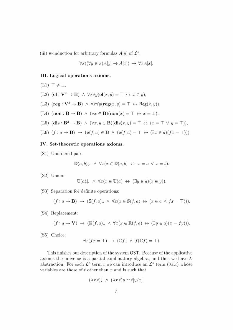
(iii) ∈-induction for arbitrary formulas A[u] of L◦,

∀x((∀y ∈ x)A[y]→ A[x]) → ∀xA[x].

III. Logical operations axioms.

(L1) > 6= ⊥,

(L2) (el : V2 → B) ∧ ∀x∀y(el(x, y) = > ↔ x ∈ y),

(L3) (reg : V2 → B) ∧ ∀x∀y(reg(x, y) = > ↔ Reg(x, y)),

(L4) (non : B→ B) ∧ (∀x ∈ B)(non(x) = > ↔ x = ⊥),

(L5) (dis : B2 → B) ∧ (∀x, y ∈ B)(dis(x, y) = > ↔ (x = > ∨ y = >)),

(L6) (f : a→ B) → (e(f, a) ∈ B ∧ (e(f, a) = > ↔ (∃x ∈ a)(fx = >))).

IV. Set-theoretic operations axioms.

(S1) Unordered pair:

D(a, b)↓ ∧ ∀x(x ∈ D(a, b) ↔ x = a ∨ x = b).

(S2) Union:U(a)↓ ∧ ∀x(x ∈ U(a) ↔ (∃y ∈ a)(x ∈ y)).

(S3) Separation for definite operations:

(f : a→ B) → (S(f, a)↓ ∧ ∀x(x ∈ S(f, a) ↔ (x ∈ a ∧ fx = >))).

(S4) Replacement:

(f : a→ V) → (R(f, a)↓ ∧ ∀x(x ∈ R(f, a) ↔ (∃y ∈ a)(x = fy))).

(S5) Choice:∃x(fx = >) → (Cf↓ ∧ f(Cf) = >).

This finishes our description of the system OST. Because of the applicativeaxioms the universe is a partial combinatory algebra, and thus we have λ-abstraction: For each L◦ term t we can introduce an L◦ term (λx.t) whosevariables are those of t other than x and is such that

(λx.t)↓ ∧ (λx.t)y ' t[y/x].

5

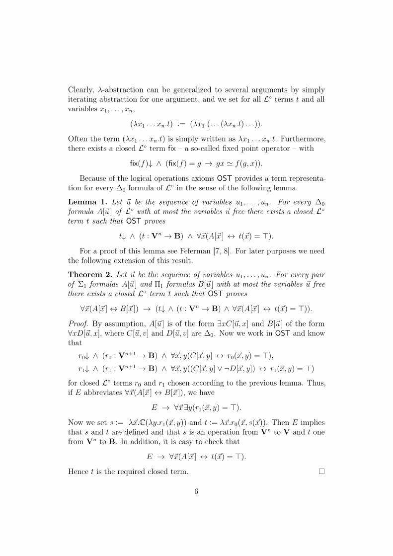
Clearly, λ-abstraction can be generalized to several arguments by simplyiterating abstraction for one argument, and we set for all L◦ terms t and allvariables x1, . . . , xn,

(λx1 . . . xn.t) := (λx1.(. . . (λxn.t) . . .)).

Often the term (λx1 . . . xn.t) is simply written as λx1 . . . xn.t. Furthermore,there exists a closed L◦ term fix – a so-called fixed point operator – with

fix(f)↓ ∧ (fix(f) = g → gx ' f(g, x)).

Because of the logical operations axioms OST provides a term representa-tion for every ∆0 formula of L◦ in the sense of the following lemma.

Lemma 1. Let ~u be the sequence of variables u1, . . . , un. For every ∆0

formula A[~u ] of L◦ with at most the variables ~u free there exists a closed L◦term t such that OST proves

t↓ ∧ (t : Vn → B) ∧ ∀~x(A[~x ] ↔ t(~x) = >).

For a proof of this lemma see Feferman [7, 8]. For later purposes we needthe following extension of this result.

Theorem 2. Let ~u be the sequence of variables u1, . . . , un. For every pairof Σ1 formulas A[~u ] and Π1 formulas B[~u ] with at most the variables ~u freethere exists a closed L◦ term t such that OST proves

∀~x(A[~x ]↔ B[~x ]) → (t↓ ∧ (t : Vn → B) ∧ ∀~x(A[~x ] ↔ t(~x) = >)).

Proof. By assumption, A[~u ] is of the form ∃xC[~u, x] and B[~u ] of the form∀xD[~u, x], where C[~u, v] and D[~u, v] are ∆0. Now we work in OST and knowthat

r0↓ ∧ (r0 : Vn+1 → B) ∧ ∀~x, y(C[~x, y] ↔ r0(~x, y) = >),

r1↓ ∧ (r1 : Vn+1 → B) ∧ ∀~x, y((C[~x, y] ∨ ¬D[~x, y]) ↔ r1(~x, y) = >)

for closed L◦ terms r0 and r1 chosen according to the previous lemma. Thus,if E abbreviates ∀~x(A[~x ]↔ B[~x ]), we have

E → ∀~x∃y(r1(~x, y) = >).

Now we set s := λ~x.C(λy.r1(~x, y)) and t := λ~x.r0(~x, s(~x)). Then E impliesthat s and t are defined and that s is an operation from Vn to V and t onefrom Vn to B. In addition, it is easy to check that

E → ∀~x(A[~x ] ↔ t(~x) = >).

Hence t is the required closed term.

6

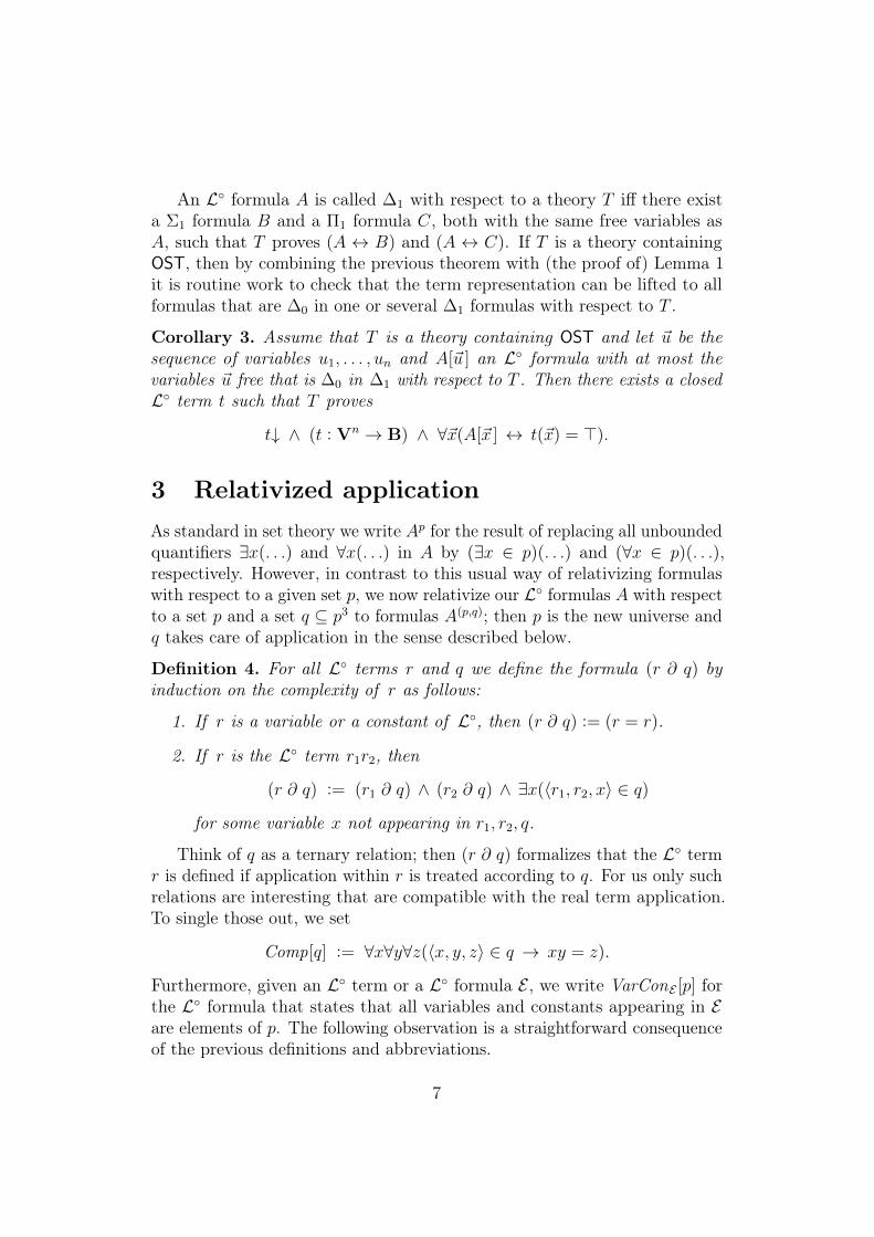
An L◦ formula A is called ∆1 with respect to a theory T iff there exista Σ1 formula B and a Π1 formula C, both with the same free variables asA, such that T proves (A ↔ B) and (A ↔ C). If T is a theory containingOST, then by combining the previous theorem with (the proof of) Lemma 1it is routine work to check that the term representation can be lifted to allformulas that are ∆0 in one or several ∆1 formulas with respect to T .

Corollary 3. Assume that T is a theory containing OST and let ~u be thesequence of variables u1, . . . , un and A[~u ] an L◦ formula with at most thevariables ~u free that is ∆0 in ∆1 with respect to T . Then there exists a closedL◦ term t such that T proves

t↓ ∧ (t : Vn → B) ∧ ∀~x(A[~x ] ↔ t(~x) = >).

3 Relativized applicationAs standard in set theory we write Ap for the result of replacing all unboundedquantifiers ∃x(. . .) and ∀x(. . .) in A by (∃x ∈ p)(. . .) and (∀x ∈ p)(. . .),respectively. However, in contrast to this usual way of relativizing formulaswith respect to a given set p, we now relativize our L◦ formulas A with respectto a set p and a set q ⊆ p3 to formulas A(p,q); then p is the new universe andq takes care of application in the sense described below.

Definition 4. For all L◦ terms r and q we define the formula (r ∂ q) byinduction on the complexity of r as follows:

1. If r is a variable or a constant of L◦, then (r ∂ q) := (r = r).

2. If r is the L◦ term r1r2, then

(r ∂ q) := (r1 ∂ q) ∧ (r2 ∂ q) ∧ ∃x(〈r1, r2, x〉 ∈ q)

for some variable x not appearing in r1, r2, q.

Think of q as a ternary relation; then (r ∂ q) formalizes that the L◦ termr is defined if application within r is treated according to q. For us only suchrelations are interesting that are compatible with the real term application.To single those out, we set

Comp[q] := ∀x∀y∀z(〈x, y, z〉 ∈ q → xy = z).

Furthermore, given an L◦ term or a L◦ formula E , we write VarConE [p] forthe L◦ formula that states that all variables and constants appearing in Eare elements of p. The following observation is a straightforward consequenceof the previous definitions and abbreviations.

7

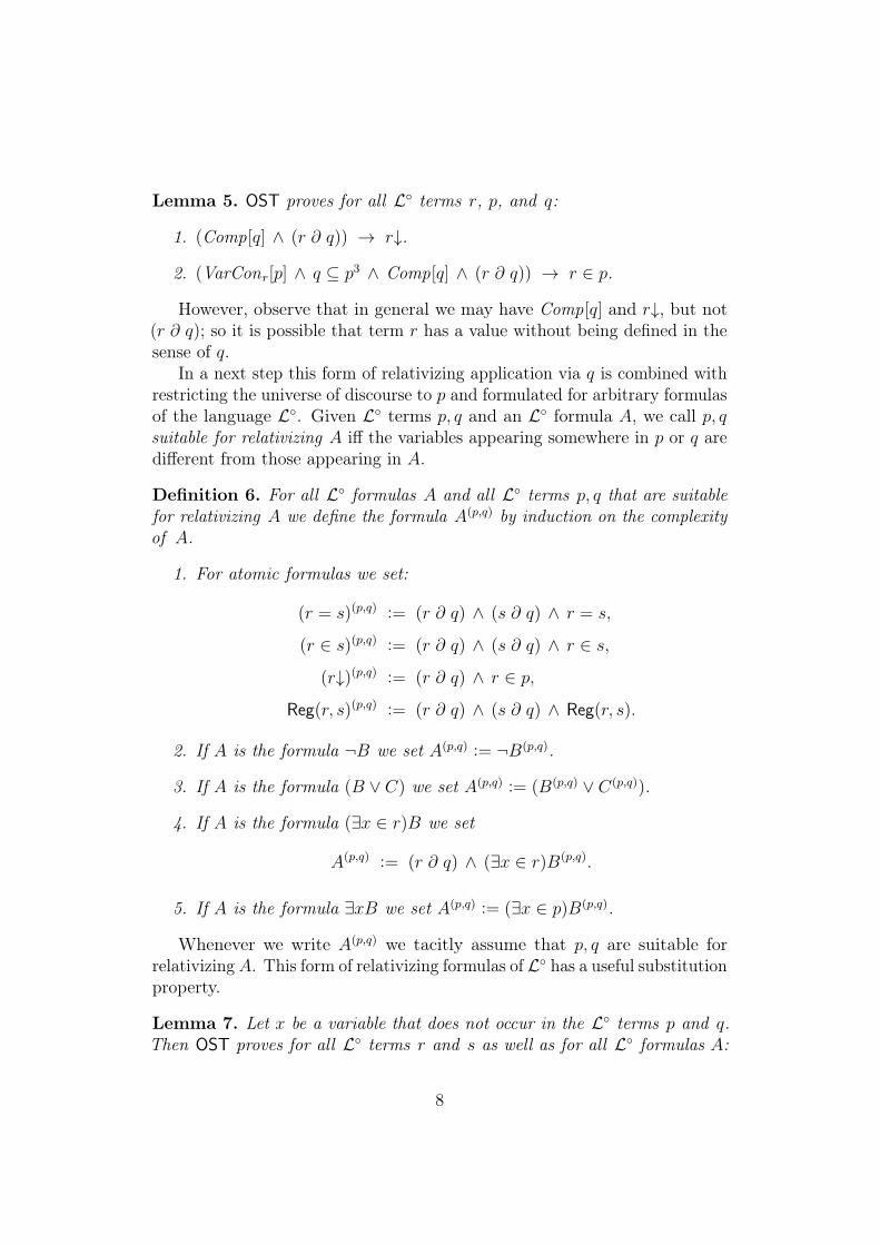
Lemma 5. OST proves for all L◦ terms r, p, and q:

1. (Comp[q] ∧ (r ∂ q)) → r↓.

2. (VarConr[p] ∧ q ⊆ p3 ∧ Comp[q] ∧ (r ∂ q)) → r ∈ p.

However, observe that in general we may have Comp[q] and r↓, but not(r ∂ q); so it is possible that term r has a value without being defined in thesense of q.

In a next step this form of relativizing application via q is combined withrestricting the universe of discourse to p and formulated for arbitrary formulasof the language L◦. Given L◦ terms p, q and an L◦ formula A, we call p, qsuitable for relativizing A iff the variables appearing somewhere in p or q aredifferent from those appearing in A.

Definition 6. For all L◦ formulas A and all L◦ terms p, q that are suitablefor relativizing A we define the formula A(p,q) by induction on the complexityof A.

1. For atomic formulas we set:

(r = s)(p,q) := (r ∂ q) ∧ (s ∂ q) ∧ r = s,

(r ∈ s)(p,q) := (r ∂ q) ∧ (s ∂ q) ∧ r ∈ s,

(r↓)(p,q) := (r ∂ q) ∧ r ∈ p,

Reg(r, s)(p,q) := (r ∂ q) ∧ (s ∂ q) ∧ Reg(r, s).

2. If A is the formula ¬B we set A(p,q) := ¬B(p,q).

3. If A is the formula (B ∨ C) we set A(p,q) := (B(p,q) ∨ C(p,q)).

4. If A is the formula (∃x ∈ r)B we set

A(p,q) := (r ∂ q) ∧ (∃x ∈ r)B(p,q).

5. If A is the formula ∃xB we set A(p,q) := (∃x ∈ p)B(p,q).

Whenever we write A(p,q) we tacitly assume that p, q are suitable forrelativizing A. This form of relativizing formulas of L◦ has a useful substitutionproperty.

Lemma 7. Let x be a variable that does not occur in the L◦ terms p and q.Then OST proves for all L◦ terms r and s as well as for all L◦ formulas A:

8

1. (Comp[q] ∧ (r ∂ q)) → ((s[r/x] ∂ q) ↔ (s ∂ q)[r/x]).

2. (Comp[q] ∧ (r ∂ q)) → (A[r/x](p,q) ↔ A(p,q)[r/x]).

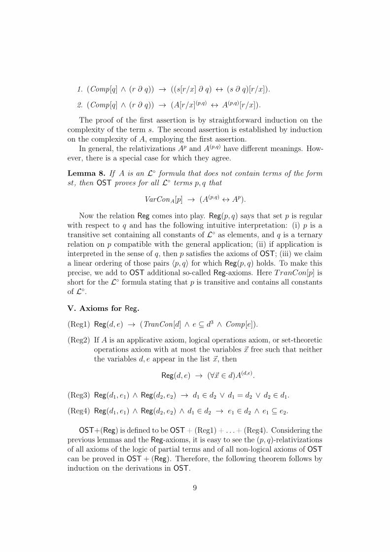
The proof of the first assertion is by straightforward induction on thecomplexity of the term s. The second assertion is established by inductionon the complexity of A, employing the first assertion.

In general, the relativizations Ap and A(p,q) have different meanings. How-ever, there is a special case for which they agree.

Lemma 8. If A is an L◦ formula that does not contain terms of the formst, then OST proves for all L◦ terms p, q that

VarConA[p] → (A(p,q) ↔ Ap).

Now the relation Reg comes into play. Reg(p, q) says that set p is regularwith respect to q and has the following intuitive interpretation: (i) p is atransitive set containing all constants of L◦ as elements, and q is a ternaryrelation on p compatible with the general application; (ii) if application isinterpreted in the sense of q, then p satisfies the axioms of OST; (iii) we claima linear ordering of those pairs 〈p, q〉 for which Reg(p, q) holds. To make thisprecise, we add to OST additional so-called Reg-axioms. Here TranCon[p] isshort for the L◦ formula stating that p is transitive and contains all constantsof L◦.

V. Axioms for Reg.

(Reg1) Reg(d, e) → (TranCon[d] ∧ e ⊆ d3 ∧ Comp[e]).

(Reg2) If A is an applicative axiom, logical operations axiom, or set-theoreticoperations axiom with at most the variables ~x free such that neitherthe variables d, e appear in the list ~x, then

Reg(d, e) → (∀~x ∈ d)A(d,e).

(Reg3) Reg(d1, e1) ∧ Reg(d2, e2) → d1 ∈ d2 ∨ d1 = d2 ∨ d2 ∈ d1.

(Reg4) Reg(d1, e1) ∧ Reg(d2, e2) ∧ d1 ∈ d2 → e1 ∈ d2 ∧ e1 ⊆ e2.

OST+(Reg) is defined to be OST + (Reg1) + . . . + (Reg4). Considering theprevious lemmas and the Reg-axioms, it is easy to see the (p, q)-relativizationsof all axioms of the logic of partial terms and of all non-logical axioms of OSTcan be proved in OST + (Reg). Therefore, the following theorem follows byinduction on the derivations in OST.

9

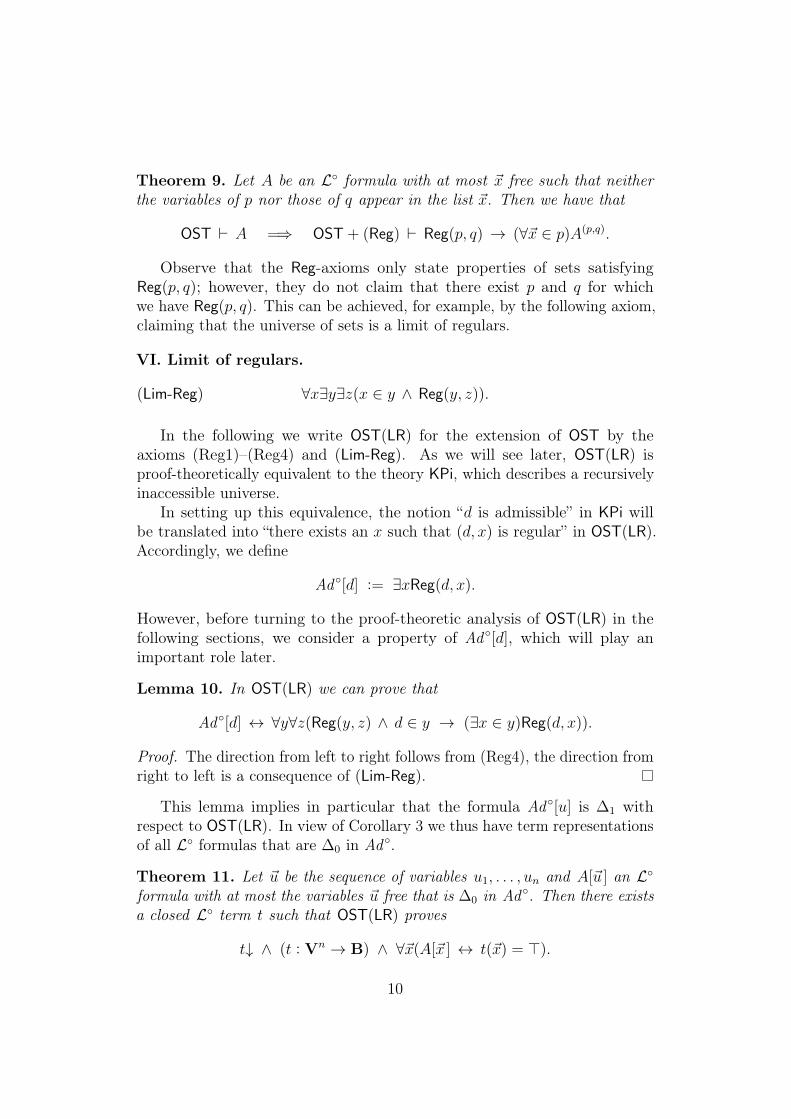
Theorem 9. Let A be an L◦ formula with at most ~x free such that neitherthe variables of p nor those of q appear in the list ~x. Then we have that

OST ` A =⇒ OST + (Reg) ` Reg(p, q) → (∀~x ∈ p)A(p,q).

Observe that the Reg-axioms only state properties of sets satisfyingReg(p, q); however, they do not claim that there exist p and q for whichwe have Reg(p, q). This can be achieved, for example, by the following axiom,claiming that the universe of sets is a limit of regulars.

VI. Limit of regulars.

(Lim-Reg) ∀x∃y∃z(x ∈ y ∧ Reg(y, z)).

In the following we write OST(LR) for the extension of OST by theaxioms (Reg1)–(Reg4) and (Lim-Reg). As we will see later, OST(LR) isproof-theoretically equivalent to the theory KPi, which describes a recursivelyinaccessible universe.

In setting up this equivalence, the notion “d is admissible” in KPi willbe translated into “there exists an x such that (d, x) is regular” in OST(LR).Accordingly, we define

Ad◦[d] := ∃xReg(d, x).

However, before turning to the proof-theoretic analysis of OST(LR) in thefollowing sections, we consider a property of Ad◦[d], which will play animportant role later.

Lemma 10. In OST(LR) we can prove that

Ad◦[d] ↔ ∀y∀z(Reg(y, z) ∧ d ∈ y → (∃x ∈ y)Reg(d, x)).

Proof. The direction from left to right follows from (Reg4), the direction fromright to left is a consequence of (Lim-Reg).

This lemma implies in particular that the formula Ad◦[u] is ∆1 withrespect to OST(LR). In view of Corollary 3 we thus have term representationsof all L◦ formulas that are ∆0 in Ad◦.

Theorem 11. Let ~u be the sequence of variables u1, . . . , un and A[~u ] an L◦formula with at most the variables ~u free that is ∆0 in Ad◦. Then there existsa closed L◦ term t such that OST(LR) proves

t↓ ∧ (t : Vn → B) ∧ ∀~x(A[~x ] ↔ t(~x) = >).

10

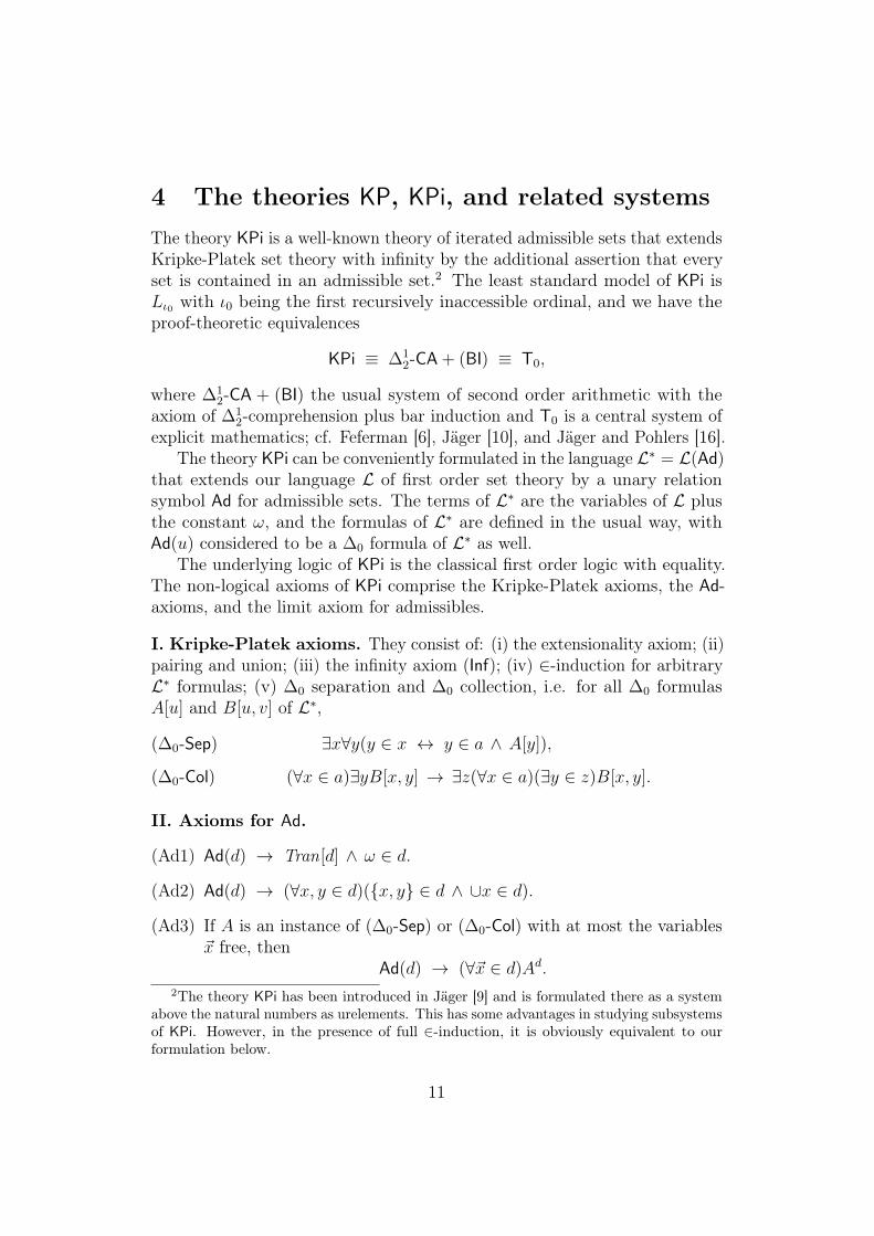
4 The theories KP, KPi, and related systemsThe theory KPi is a well-known theory of iterated admissible sets that extendsKripke-Platek set theory with infinity by the additional assertion that everyset is contained in an admissible set.2 The least standard model of KPi isLι0 with ι0 being the first recursively inaccessible ordinal, and we have theproof-theoretic equivalences

KPi ≡ ∆12-CA + (BI) ≡ T0,

where ∆12-CA + (BI) the usual system of second order arithmetic with the

axiom of ∆12-comprehension plus bar induction and T0 is a central system of

explicit mathematics; cf. Feferman [6], Jäger [10], and Jäger and Pohlers [16].The theory KPi can be conveniently formulated in the language L∗ = L(Ad)

that extends our language L of first order set theory by a unary relationsymbol Ad for admissible sets. The terms of L∗ are the variables of L plusthe constant ω, and the formulas of L∗ are defined in the usual way, withAd(u) considered to be a ∆0 formula of L∗ as well.

The underlying logic of KPi is the classical first order logic with equality.The non-logical axioms of KPi comprise the Kripke-Platek axioms, the Ad-axioms, and the limit axiom for admissibles.

I. Kripke-Platek axioms. They consist of: (i) the extensionality axiom; (ii)pairing and union; (iii) the infinity axiom (Inf); (iv) ∈-induction for arbitraryL∗ formulas; (v) ∆0 separation and ∆0 collection, i.e. for all ∆0 formulasA[u] and B[u, v] of L∗,

∃x∀y(y ∈ x ↔ y ∈ a ∧ A[y]),(∆0-Sep)

(∀x ∈ a)∃yB[x, y] → ∃z(∀x ∈ a)(∃y ∈ z)B[x, y].(∆0-Col)

II. Axioms for Ad.

(Ad1) Ad(d) → Tran[d] ∧ ω ∈ d.

(Ad2) Ad(d) → (∀x, y ∈ d)({x, y} ∈ d ∧ ∪x ∈ d).

(Ad3) If A is an instance of (∆0-Sep) or (∆0-Col) with at most the variables~x free, then

Ad(d) → (∀~x ∈ d)Ad.2The theory KPi has been introduced in Jäger [9] and is formulated there as a system

above the natural numbers as urelements. This has some advantages in studying subsystemsof KPi. However, in the presence of full ∈-induction, it is obviously equivalent to ourformulation below.

11

(Ad4) Ad(d1) ∧ Ad(d2) → d1 ∈ d2 ∨ d1 = d2 ∨ d2 ∈ d1.

III. Limit of admissibles.

(Lim-Ad) ∀x∃y(x ∈ y ∧ Ad(y)).

Kripke-Platek set theory KP is the subsystem of KPi obtained from KPiby deleting the axiom (Lim-Ad). Clearly, the axioms for Ad imply that everyset satisfying Ad is transitive, contains ω and is closed under pairing, union,∆0 separation and ∆0 collection. Together with the axiom (Lim-Ad) we thusknow that every model of KPi is an admissible limit of admissibles.

By KPi we denote the subsystem of KPi that is obtained from KPi byrestricting the axioms (Ad3) to formulas of L, i.e. to formulas not containingthe relation symbol Ad. It is easy to see that KPi is of the same proof-theoreticstrength as KPi. For example, the embedding of ∆1

2-CA + (BI) into KPi, aspresented in Jäger [11], also works for KPi.

Following standard terminology, we call a formula A of L∗ a ∆(KP) formulaiff there exist a Σ formula B and a Π formula C of L∗, both with the samefree variables as A, such that

KP ` (A↔ B) ∧ (A↔ C).

The constructible hierarchy provides for important examples of ∆(KP) for-mulas. We cannot introduce it here but refer for all relevant details to, forexample, Barwise [1] or Kunen [19]. All we need is that (a ∈ Lα) states thatthe set a is an element of the α-th level Lα of the constructible hierarchyand (a ∈ L) is short for ∃α(a ∈ Lα); besides that (a <L b) means that a issmaller than b according to the well-ordering <L on the constructible universeL. The axiom of constructibility is the statement (V = L), i.e. ∀x(x ∈ L). Itis well-known that the assertions (a ∈ Lα) and (a <L b) are ∆(KP) formulas.In addition, the theories KP + (V=L) and KPi + (V=L) are of the sameconsistency strength as KP and KPi, respectively.

In the following we write d |= pKPq to state that d is a transitive standardmodel of KP and refer to Barwise [1] and Probst [20] for details. Then we set

AdL[d] := ∃ξ(Limit [ξ] ∧ d = Lξ) ∧ d |= pKPq.

If d satisfies AdL[d], we call it an L-admissible set. Since KP proves theequivalence of the assertion ∃ξ(Limit [ξ] ∧ d = Lξ) with

∅ ∈ d ∧ Tran[d] ∧ (∀x ∈ d)(∃ξ ∈ d)(x ∈ Lξ ∧ Lξ ∈ d),

we conclude that AdL[d] is a ∆(KP) formula. The first assertion of thefollowing lemma is immediate from the definition of AdL, the second follows

12

from the first and some obvious persistency arguments, and the third is byan inner model construction; see again [1, 20].

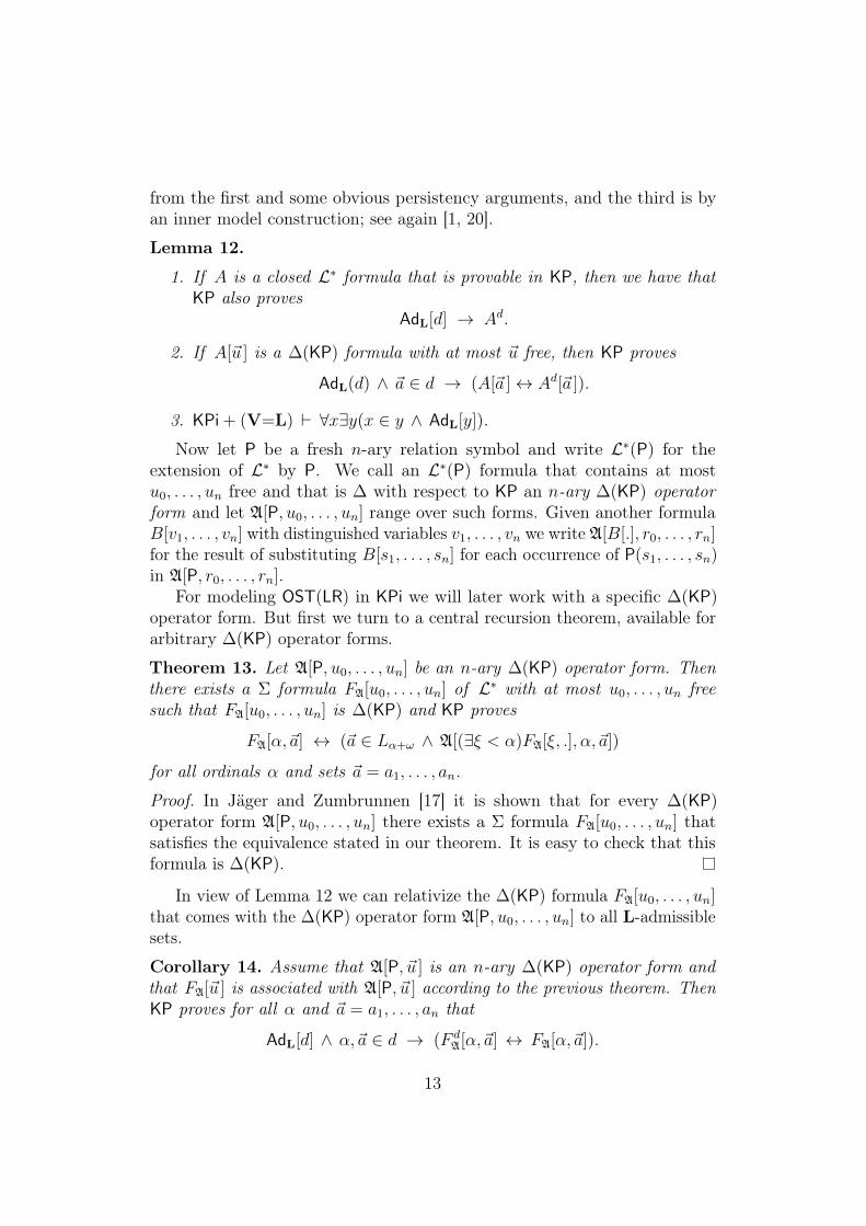
Lemma 12.

1. If A is a closed L∗ formula that is provable in KP, then we have thatKP also proves

AdL[d] → Ad.

2. If A[~u ] is a ∆(KP) formula with at most ~u free, then KP proves

AdL(d) ∧ ~a ∈ d → (A[~a ]↔ Ad[~a ]).

3. KPi + (V=L) ` ∀x∃y(x ∈ y ∧ AdL[y]).

Now let P be a fresh n-ary relation symbol and write L∗(P) for theextension of L∗ by P. We call an L∗(P) formula that contains at mostu0, . . . , un free and that is ∆ with respect to KP an n-ary ∆(KP) operatorform and let A[P, u0, . . . , un] range over such forms. Given another formulaB[v1, . . . , vn] with distinguished variables v1, . . . , vn we write A[B[.], r0, . . . , rn]for the result of substituting B[s1, . . . , sn] for each occurrence of P(s1, . . . , sn)in A[P, r0, . . . , rn].

For modeling OST(LR) in KPi we will later work with a specific ∆(KP)operator form. But first we turn to a central recursion theorem, available forarbitrary ∆(KP) operator forms.

Theorem 13. Let A[P, u0, . . . , un] be an n-ary ∆(KP) operator form. Thenthere exists a Σ formula FA[u0, . . . , un] of L∗ with at most u0, . . . , un freesuch that FA[u0, . . . , un] is ∆(KP) and KP proves

FA[α,~a] ↔ (~a ∈ Lα+ω ∧ A[(∃ξ < α)FA[ξ, .], α,~a])

for all ordinals α and sets ~a = a1, . . . , an.

Proof. In Jäger and Zumbrunnen [17] it is shown that for every ∆(KP)operator form A[P, u0, . . . , un] there exists a Σ formula FA[u0, . . . , un] thatsatisfies the equivalence stated in our theorem. It is easy to check that thisformula is ∆(KP).

In view of Lemma 12 we can relativize the ∆(KP) formula FA[u0, . . . , un]that comes with the ∆(KP) operator form A[P, u0, . . . , un] to all L-admissiblesets.

Corollary 14. Assume that A[P, ~u ] is an n-ary ∆(KP) operator form andthat FA[~u ] is associated with A[P, ~u ] according to the previous theorem. ThenKP proves for all α and ~a = a1, . . . , an that

AdL[d] ∧ α,~a ∈ d → (F dA[α,~a] ↔ FA[α,~a]).

13

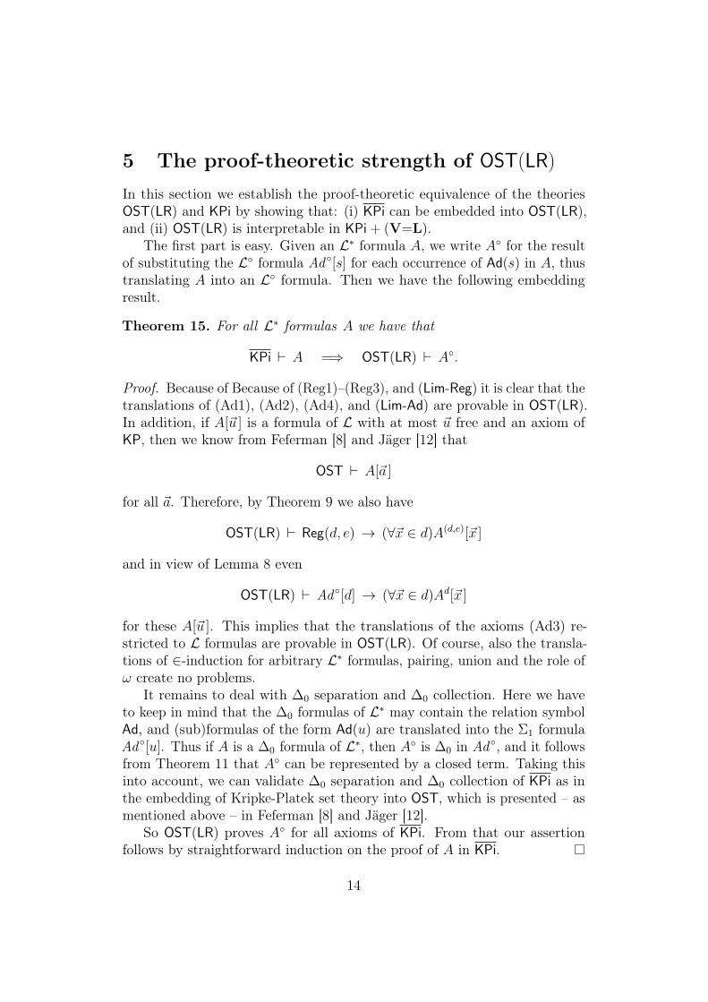
5 The proof-theoretic strength of OST(LR)In this section we establish the proof-theoretic equivalence of the theoriesOST(LR) and KPi by showing that: (i) KPi can be embedded into OST(LR),and (ii) OST(LR) is interpretable in KPi + (V=L).

The first part is easy. Given an L∗ formula A, we write A◦ for the resultof substituting the L◦ formula Ad◦[s] for each occurrence of Ad(s) in A, thustranslating A into an L◦ formula. Then we have the following embeddingresult.

Theorem 15. For all L∗ formulas A we have that

KPi ` A =⇒ OST(LR) ` A◦.

Proof. Because of Because of (Reg1)–(Reg3), and (Lim-Reg) it is clear that thetranslations of (Ad1), (Ad2), (Ad4), and (Lim-Ad) are provable in OST(LR).In addition, if A[~u ] is a formula of L with at most ~u free and an axiom ofKP, then we know from Feferman [8] and Jäger [12] that

OST ` A[~a ]

for all ~a. Therefore, by Theorem 9 we also have

OST(LR) ` Reg(d, e) → (∀~x ∈ d)A(d,e)[~x ]

and in view of Lemma 8 even

OST(LR) ` Ad◦[d] → (∀~x ∈ d)Ad[~x ]

for these A[~u ]. This implies that the translations of the axioms (Ad3) re-stricted to L formulas are provable in OST(LR). Of course, also the transla-tions of ∈-induction for arbitrary L∗ formulas, pairing, union and the role ofω create no problems.

It remains to deal with ∆0 separation and ∆0 collection. Here we haveto keep in mind that the ∆0 formulas of L∗ may contain the relation symbolAd, and (sub)formulas of the form Ad(u) are translated into the Σ1 formulaAd◦[u]. Thus if A is a ∆0 formula of L∗, then A◦ is ∆0 in Ad◦, and it followsfrom Theorem 11 that A◦ can be represented by a closed term. Taking thisinto account, we can validate ∆0 separation and ∆0 collection of KPi as inthe embedding of Kripke-Platek set theory into OST, which is presented – asmentioned above – in Feferman [8] and Jäger [12].

So OST(LR) proves A◦ for all axioms of KPi. From that our assertionfollows by straightforward induction on the proof of A in KPi.

14

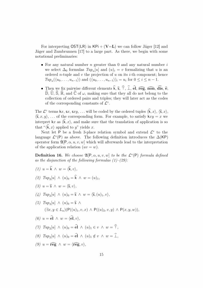
For interpreting OST(LR) in KPi + (V=L) we can follow Jäger [12] andJäger and Zumbrunnen [17] to a large part. As there, we begin with somenotational preliminaries:

• For any natural number n greater than 0 and any natural number iwe select ∆0 formulas Tupn[u] and (u)i = v formalizing that u is anordered n-tuple and v the projection of u on its i-th component; henceTupn(〈u0, . . . , un−1〉) and (〈u0, . . . , un−1〉)i = ui for 0 ≤ i ≤ n− 1.

• Then we fix pairwise different elements k, s, >, ⊥, el, reg, non, dis, e,D, U, S, R, and C of ω, making sure that they all do not belong to thecollection of ordered pairs and triples; they will later act as the codesof the corresponding constants of L◦.

The L◦ terms kx, sx, sxy, . . . will be coded by the ordered tuples 〈k, x〉, 〈s, x〉,〈s, x, y〉, . . . of the corresponding form. For example, to satisfy kxy = x weinterpret kx as 〈k, x〉, and make sure that the translation of application is sothat “〈k, x〉 applied to y” yields x.

Next let P be a fresh 3-place relation symbol and extend L∗ to thelanguage L∗(P) as above. The following definition introduces the ∆(KP)operator form A[P, α, u, v, w] which will afterwards lead to the interpretationof the application relation (uv = w).

Definition 16. We choose A[P, α, u, v, w] to be the L∗(P) formula definedas the disjunction of the following formulas (1)–(29):

(1) u = k ∧ w = 〈k, v〉,

(2) Tup2[u] ∧ (u)0 = k ∧ w = (u)1,

(3) u = s ∧ w = 〈s, v〉,

(4) Tup2[u] ∧ (u)0 = s ∧ w = 〈s, (u)1, v〉,

(5) Tup3[u] ∧ (u)0 = s ∧(∃x, y ∈ Lα)(P((u)1, v, x) ∧ P((u)2, v, y) ∧ P(x, y, w)),

(6) u = el ∧ w = 〈el, v〉,

(7) Tup2[u] ∧ (u)0 = el ∧ (u)1 ∈ v ∧ w = >,

(8) Tup2[u] ∧ (u)0 = el ∧ (u)1 /∈ v ∧ w = ⊥,

(9) u = reg ∧ w = 〈reg, v〉,

15

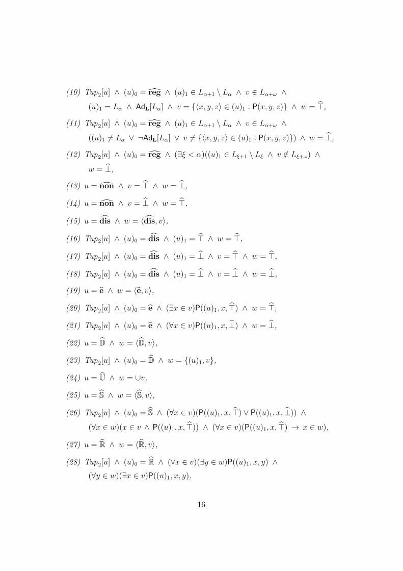
(10) Tup2[u] ∧ (u)0 = reg ∧ (u)1 ∈ Lα+1 \ Lα ∧ v ∈ Lα+ω ∧

(u)1 = Lα ∧ AdL[Lα] ∧ v = {〈x, y, z〉 ∈ (u)1 : P(x, y, z)} ∧ w = >,

(11) Tup2[u] ∧ (u)0 = reg ∧ (u)1 ∈ Lα+1 \ Lα ∧ v ∈ Lα+ω ∧

((u)1 6= Lα ∨ ¬AdL[Lα] ∨ v 6= {〈x, y, z〉 ∈ (u)1 : P(x, y, z)}) ∧ w = ⊥,

(12) Tup2[u] ∧ (u)0 = reg ∧ (∃ξ < α)((u)1 ∈ Lξ+1 \ Lξ ∧ v /∈ Lξ+ω) ∧

w = ⊥,

(13) u = non ∧ v = > ∧ w = ⊥,

(14) u = non ∧ v = ⊥ ∧ w = >,

(15) u = dis ∧ w = 〈dis, v〉,

(16) Tup2[u] ∧ (u)0 = dis ∧ (u)1 = > ∧ w = >,

(17) Tup2[u] ∧ (u)0 = dis ∧ (u)1 = ⊥ ∧ v = > ∧ w = >,

(18) Tup2[u] ∧ (u)0 = dis ∧ (u)1 = ⊥ ∧ v = ⊥ ∧ w = ⊥,

(19) u = e ∧ w = 〈e, v〉,

(20) Tup2[u] ∧ (u)0 = e ∧ (∃x ∈ v)P((u)1, x, >) ∧ w = >,

(21) Tup2[u] ∧ (u)0 = e ∧ (∀x ∈ v)P((u)1, x, ⊥) ∧ w = ⊥,

(22) u = D ∧ w = 〈D, v〉,

(23) Tup2[u] ∧ (u)0 = D ∧ w = {(u)1, v},

(24) u = U ∧ w = ∪v,

(25) u = S ∧ w = 〈S, v〉,

(26) Tup2[u] ∧ (u)0 = S ∧ (∀x ∈ v)(P((u)1, x, >) ∨ P((u)1, x, ⊥)) ∧

(∀x ∈ w)(x ∈ v ∧ P((u)1, x, >)) ∧ (∀x ∈ v)(P((u)1, x, >) → x ∈ w),

(27) u = R ∧ w = 〈R, v〉,

(28) Tup2[u] ∧ (u)0 = R ∧ (∀x ∈ v)(∃y ∈ w)P((u)1, x, y) ∧(∀y ∈ w)(∃x ∈ v)P((u)1, x, y),

16

(29) u = C ∧ P(v, w, >) ∧ (∀x ∈ Lα)(x <L w → ¬P(v, x, >)) ∧

(∀x ∈ Lα)¬P(C, v, x).

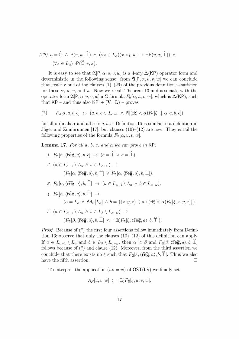
It is easy to see that A[P, α, u, v, w] is a 4-ary ∆(KP) operator form anddeterministic in the following sense: from A[P, α, u, v, w] we can concludethat exactly one of the clauses (1)–(29) of the previous definition is satisfiedfor these α, u, v, and w. Now we recall Theorem 13 and associate with theoperator form A[P, α, u, v, w] a Σ formula FA[α, u, v, w], which is ∆(KP), suchthat KP – and thus also KPi + (V=L) – proves

(*) FA[α, a, b, c] ↔ (a, b, c ∈ Lα+ω ∧ A[(∃ξ < α)FA[ξ, .], α, a, b, c])

for all ordinals α and all sets a, b, c. Definition 16 is similar to a definition inJäger and Zumbrunnen [17], but clauses (10)–(12) are new. They entail thefollowing properties of the formula FA[α, u, v, w].

Lemma 17. For all a, b, c, and α we can prove in KP:

1. FA[α, 〈reg, a〉, b, c] → (c = > ∨ c = ⊥).

2. (a ∈ Lα+1 \ Lα ∧ b ∈ Lα+ω) →

(FA[α, 〈reg, a〉, b, >] ∨ FA[α, 〈reg, a〉, b, ⊥]).

3. FA[α, 〈reg, a〉, b, >] → (a ∈ Lα+1 \ Lα ∧ b ∈ Lα+ω).

4. FA[α, 〈reg, a〉, b, >] →(a = Lα ∧ AdL[Lα] ∧ b = {〈x, y, z〉 ∈ a : (∃ξ < α)FA[ξ, x, y, z]}).

5. (a ∈ Lα+1 \ Lα ∧ b ∈ Lβ \ Lα+ω) →

(FA[β, 〈reg, a〉, b, ⊥] ∧ ¬∃ξFA[ξ, 〈reg, a〉, b, >]).

Proof. Because of (*) the first four assertions follow immediately from Defini-tion 16; observe that only the clauses (10)–(12) of this definition can apply.If a ∈ Lα+1 \ Lα and b ∈ Lβ \ Lα+ω, then α < β and FA[β, 〈reg, a〉, b, ⊥]follows because of (*) and clause (12). Moreover, from the third assertion weconclude that there exists no ξ such that FA[ξ, 〈reg, a〉, b, >]. Thus we alsohave the fifth assertion.

To interpret the application (uv = w) of OST(LR) we finally set

Ap[u, v, w] := ∃ξFA[ξ, u, v, w].

17

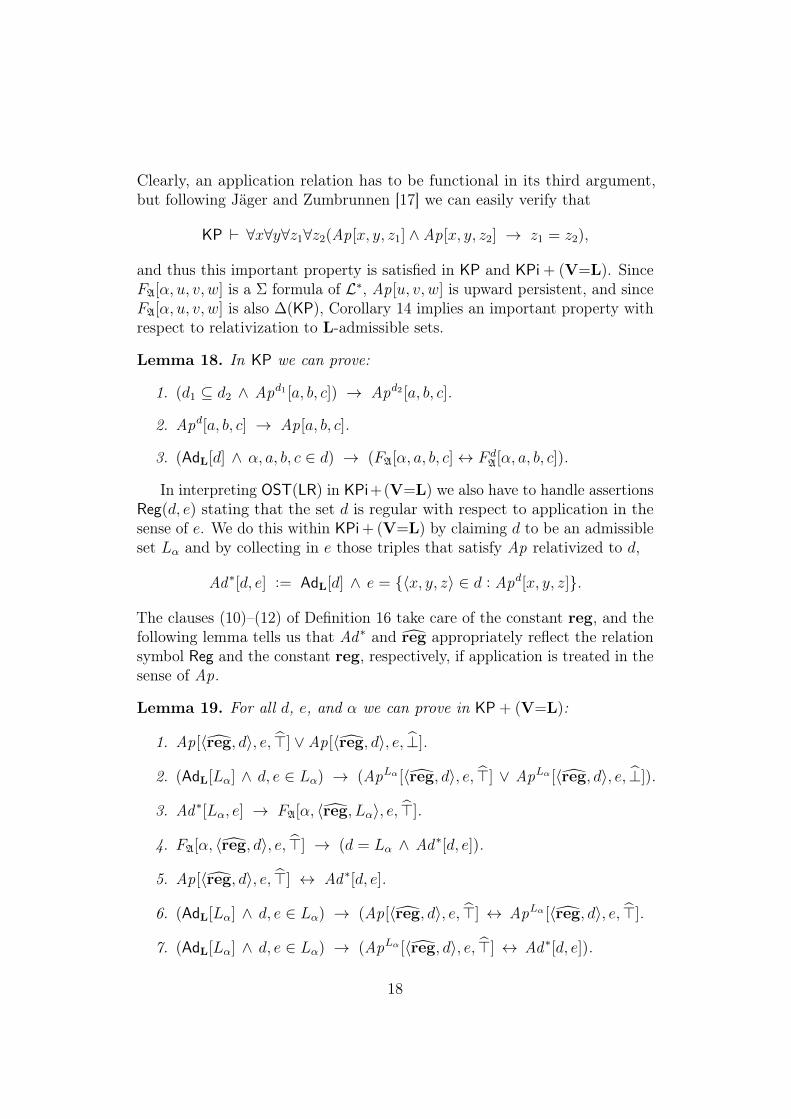
Clearly, an application relation has to be functional in its third argument,but following Jäger and Zumbrunnen [17] we can easily verify that

KP ` ∀x∀y∀z1∀z2(Ap[x, y, z1] ∧ Ap[x, y, z2] → z1 = z2),

and thus this important property is satisfied in KP and KPi + (V=L). SinceFA[α, u, v, w] is a Σ formula of L∗, Ap[u, v, w] is upward persistent, and sinceFA[α, u, v, w] is also ∆(KP), Corollary 14 implies an important property withrespect to relativization to L-admissible sets.

Lemma 18. In KP we can prove:

1. (d1 ⊆ d2 ∧ Apd1 [a, b, c]) → Apd2 [a, b, c].

2. Apd[a, b, c] → Ap[a, b, c].

3. (AdL[d] ∧ α, a, b, c ∈ d) → (FA[α, a, b, c]↔ F dA[α, a, b, c]).

In interpreting OST(LR) in KPi+(V=L) we also have to handle assertionsReg(d, e) stating that the set d is regular with respect to application in thesense of e. We do this within KPi + (V=L) by claiming d to be an admissibleset Lα and by collecting in e those triples that satisfy Ap relativized to d,

Ad∗[d, e] := AdL[d] ∧ e = {〈x, y, z〉 ∈ d : Apd[x, y, z]}.

The clauses (10)–(12) of Definition 16 take care of the constant reg, and thefollowing lemma tells us that Ad∗ and reg appropriately reflect the relationsymbol Reg and the constant reg, respectively, if application is treated in thesense of Ap.

Lemma 19. For all d, e, and α we can prove in KP + (V=L):

1. Ap[〈reg, d〉, e, >] ∨ Ap[〈reg, d〉, e, ⊥].

2. (AdL[Lα] ∧ d, e ∈ Lα) → (ApLα [〈reg, d〉, e, >] ∨ ApLα [〈reg, d〉, e, ⊥]).

3. Ad∗[Lα, e] → FA[α, 〈reg, Lα〉, e, >].

4. FA[α, 〈reg, d〉, e, >] → (d = Lα ∧ Ad∗[d, e]).

5. Ap[〈reg, d〉, e, >] ↔ Ad∗[d, e].

6. (AdL[Lα] ∧ d, e ∈ Lα) → (Ap[〈reg, d〉, e, >] ↔ ApLα [〈reg, d〉, e, >].

7. (AdL[Lα] ∧ d, e ∈ Lα) → (ApLα [〈reg, d〉, e, >] ↔ Ad∗[d, e]).

18

Proof. Because of (V=L) we know that there exist ordinals α and β such thatd ∈ Lα+1 \ Lα and e ∈ Lβ. Hence the first assertion follows from Lemma 17.

To prove the second assertion, assume AdL[Lα] and d, e ∈ Lα. Then thereexists an ordinal γ < α for which d ∈ Lγ+1 \ Lγ, and we distinguish thefollowing two cases:

(i) e ∈ Lγ+ω. By Lemma 17 we then have

FA[γ, 〈reg, d〉, e, >] ∨ FA[γ, 〈reg, d〉, e, ⊥]

and thus Lemma 18 yields

FLαA [γ, 〈reg, d〉, e, >] ∨ FLα

A [γ, 〈reg, d〉, e, ⊥].

Consequently, we have

ApLα [〈reg, d〉, e, >] ∨ ApLα [〈reg, d〉, e, ⊥].

(ii) e /∈ Lγ+ω. Now we choose an ordinal δ < α for which e ∈ Lδ. Lemma 17now implies

FA[δ, 〈reg, d〉, e, ⊥].

Hence an application of Lemma 18 gives us

FLαA [δ, 〈reg, d〉, e, ⊥],

and ApLα [〈reg, d〉, e, ⊥] is an immediate consequence.

In both cases (i) and (ii) we have what we want, and the second assertion isproved.

To show the third assertion we assume Ad∗[Lα, e]. Then we have AdL[Lα]and

e = {〈x, y, z〉 ∈ Lα : (∃ξ < α)FLαA [ξ, x, y, z]}.

Obviously, e ∈ Lα+ω. Furthermore, by applying Lemma 18 we can concludethat

e = {〈x, y, z〉 ∈ Lα : (∃ξ < α)FA[ξ, x, y, z]}.

In view of clause (10) of Definition 16 and equivalence (*) above this impliesFA[α, 〈reg, Lα〉, e, >].

Now we turn to the fourth assertion and assume FA[α, 〈reg, d〉, e, >].Because of equivalence (*) this implies

〈reg, d〉, e, > ∈ Lα+ω ∧ A[(∃ξ < α)FA[ξ, .], α, 〈reg, d〉, e, >].

19

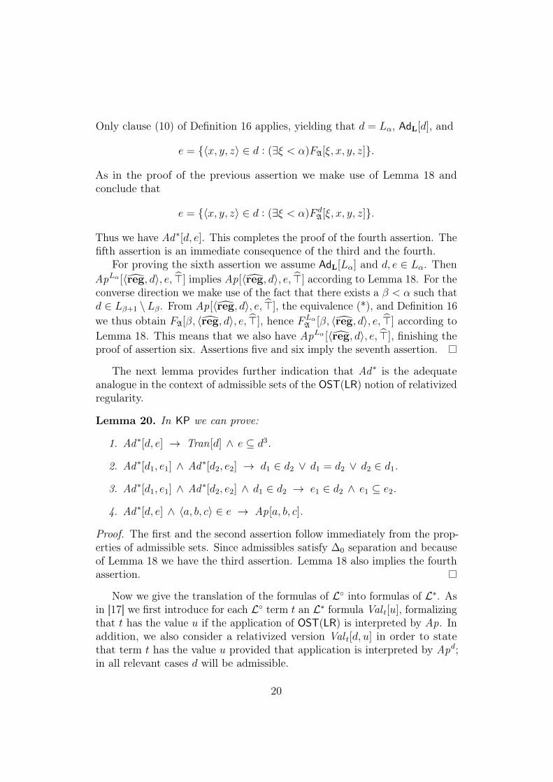
Only clause (10) of Definition 16 applies, yielding that d = Lα, AdL[d], and

e = {〈x, y, z〉 ∈ d : (∃ξ < α)FA[ξ, x, y, z]}.

As in the proof of the previous assertion we make use of Lemma 18 andconclude that

e = {〈x, y, z〉 ∈ d : (∃ξ < α)F dA[ξ, x, y, z]}.

Thus we have Ad∗[d, e]. This completes the proof of the fourth assertion. Thefifth assertion is an immediate consequence of the third and the fourth.

For proving the sixth assertion we assume AdL[Lα] and d, e ∈ Lα. ThenApLα [〈reg, d〉, e, >] implies Ap[〈reg, d〉, e, >] according to Lemma 18. For theconverse direction we make use of the fact that there exists a β < α such thatd ∈ Lβ+1 \Lβ. From Ap[〈reg, d〉, e, >], the equivalence (*), and Definition 16we thus obtain FA[β, 〈reg, d〉, e, >], hence FLα

A [β, 〈reg, d〉, e, >] according toLemma 18. This means that we also have ApLα [〈reg, d〉, e, >], finishing theproof of assertion six. Assertions five and six imply the seventh assertion.

The next lemma provides further indication that Ad∗ is the adequateanalogue in the context of admissible sets of the OST(LR) notion of relativizedregularity.

Lemma 20. In KP we can prove:

1. Ad∗[d, e] → Tran[d] ∧ e ⊆ d3.

2. Ad∗[d1, e1] ∧ Ad∗[d2, e2] → d1 ∈ d2 ∨ d1 = d2 ∨ d2 ∈ d1.

3. Ad∗[d1, e1] ∧ Ad∗[d2, e2] ∧ d1 ∈ d2 → e1 ∈ d2 ∧ e1 ⊆ e2.

4. Ad∗[d, e] ∧ 〈a, b, c〉 ∈ e → Ap[a, b, c].

Proof. The first and the second assertion follow immediately from the prop-erties of admissible sets. Since admissibles satisfy ∆0 separation and becauseof Lemma 18 we have the third assertion. Lemma 18 also implies the fourthassertion.

Now we give the translation of the formulas of L◦ into formulas of L∗. Asin [17] we first introduce for each L◦ term t an L∗ formula Val t[u], formalizingthat t has the value u if the application of OST(LR) is interpreted by Ap. Inaddition, we also consider a relativized version Val t[d, u] in order to statethat term t has the value u provided that application is interpreted by Apd;in all relevant cases d will be admissible.

20

Definition 21. For each L◦ term r and variables u and d not occurring inr we introduce L∗ formulas Val r[u] and Val r[d, u] that are inductively definedas follows:

1. If r is a variable or the constant ω, then Val r[u] and Val r[d, u] are theformula (r = u).

2. If r is another constant, then Val r[u] and Val r[d, u] are the formula(r = u).

3. If r is the term (st), then we set (for x and y chosen so that they donot occur in r)

Val r[u] := ∃x∃y(Val s[x] ∧ Val t[y] ∧ Ap[x, y, u]),

Val r[d, u] := (∃x, y ∈ d)(Val s[d, x] ∧ Val t[d, y] ∧ Apd[x, y, u]).

Notice that for every term r of L◦ its translation formula Val r[u] is a Σformula of L∗; in general, it is not ∆(KP). The translation formula Val r[d, u]is the restriction of Var r[u] to d and thus a ∆0 formula of L∗. The followingobservation is proved by induction on the buildup of r and an immediateconsequence of the functionality of Ap[u, v, w] in its third argument and ofLemma 18.

Lemma 22. KP proves for all L◦ terms r and all variables d:

1. ∀x∀y(Val r[x] ∧ Val r[y] → x = y).

2. ∀x(Val r[d, x]→ Val r[x]).

3. ∀x∀y(Val r[d, x] ∧ Val r[d, y] → x = y).

Clearly, the values of terms also satisfy the following substitution property.Again, its proof is by induction on the buildup of r.

Lemma 23. If all variables of the L◦ term r come from the list u1, . . . , unand if s is the L◦ term r[t1, . . . , tn/u1, . . . , un], then KP proves

n∧i=1

Val ti [ui] → ∀x(Val r[x] ↔ Val s[x]).

The above treatments of the application of OST(LR) determine canonicaltranslations of the formulas of L◦ into formulas of L∗.

21

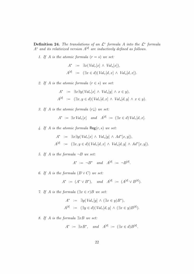
Definition 24. The translations of an L◦ formula A into the L∗ formulaA∗ and its relativized version A[d] are inductively defined as follows.

1. If A is the atomic formula (r = s) we set:

A∗ := ∃x(Val r[x] ∧ Val s[x]),

A[d] := (∃x ∈ d)(Val r[d, x] ∧ Val s[d, x]).

2. If A is the atomic formula (r ∈ s) we set:

A∗ := ∃x∃y(Val r[x] ∧ Val s[y] ∧ x ∈ y),

A[d] := (∃x, y ∈ d)(Val r[d, x] ∧ Val s[d, y] ∧ x ∈ y).

3. If A is the atomic formula (r↓) we set:

A∗ := ∃xVal r[x] and A[d] := (∃x ∈ d)Val r[d, x].

4. If A is the atomic formula Reg(r, s) we set:

A∗ := ∃x∃y(Val r[x] ∧ Val s[y] ∧ Ad∗[x, y]),

A[d] := (∃x, y ∈ d)(Val r[d, x] ∧ Val s[d, y] ∧ Ad∗[x, y]).

5. If A is the formula ¬B we set:

A∗ := ¬B∗ and A[d] := ¬B[d].

6. If A is the formula (B ∨ C) we set:

A∗ := (A∗ ∨B∗), and A[d] := (A[d] ∨B[d]).

7. If A is the formula (∃x ∈ r)B we set:

A∗ := ∃y(Val r[y] ∧ (∃x ∈ y)B∗),

A[d] := (∃y ∈ d)(Val r[d, y] ∧ (∃x ∈ y)B[d]).

8. If A is the formula ∃xB we set:

A∗ := ∃xB∗, and A[d] := (∃x ∈ d)B[d].

22

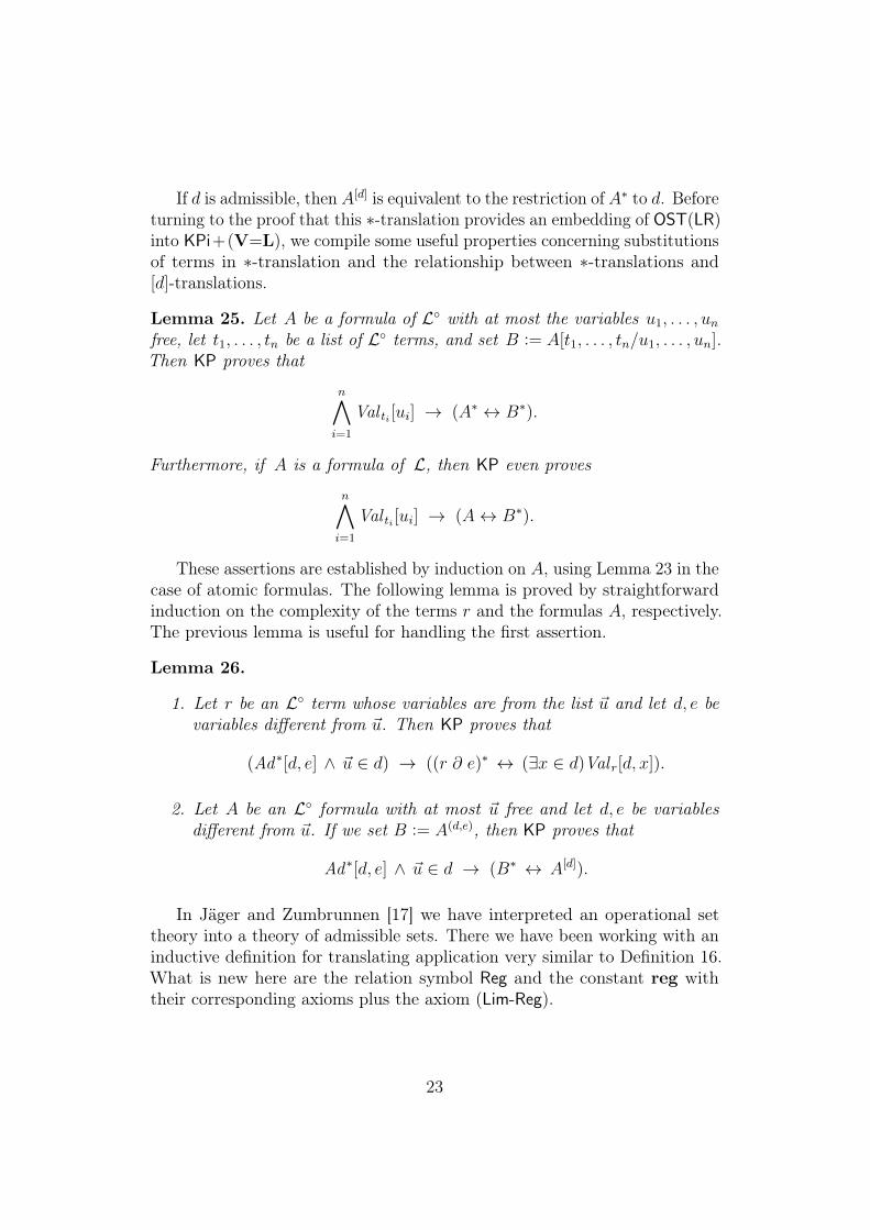
If d is admissible, then A[d] is equivalent to the restriction of A∗ to d. Beforeturning to the proof that this ∗-translation provides an embedding of OST(LR)into KPi+(V=L), we compile some useful properties concerning substitutionsof terms in ∗-translation and the relationship between ∗-translations and[d]-translations.

Lemma 25. Let A be a formula of L◦ with at most the variables u1, . . . , unfree, let t1, . . . , tn be a list of L◦ terms, and set B := A[t1, . . . , tn/u1, . . . , un].Then KP proves that

n∧i=1

Val ti [ui] → (A∗ ↔ B∗).

Furthermore, if A is a formula of L, then KP even proves

n∧i=1

Val ti [ui] → (A↔ B∗).

These assertions are established by induction on A, using Lemma 23 in thecase of atomic formulas. The following lemma is proved by straightforwardinduction on the complexity of the terms r and the formulas A, respectively.The previous lemma is useful for handling the first assertion.

Lemma 26.

1. Let r be an L◦ term whose variables are from the list ~u and let d, e bevariables different from ~u. Then KP proves that

(Ad∗[d, e] ∧ ~u ∈ d) → ((r ∂ e)∗ ↔ (∃x ∈ d)Val r[d, x]).

2. Let A be an L◦ formula with at most ~u free and let d, e be variablesdifferent from ~u. If we set B := A(d,e), then KP proves that

Ad∗[d, e] ∧ ~u ∈ d → (B∗ ↔ A[d]).

In Jäger and Zumbrunnen [17] we have interpreted an operational settheory into a theory of admissible sets. There we have been working with aninductive definition for translating application very similar to Definition 16.What is new here are the relation symbol Reg and the constant reg withtheir corresponding axioms plus the axiom (Lim-Reg).

23

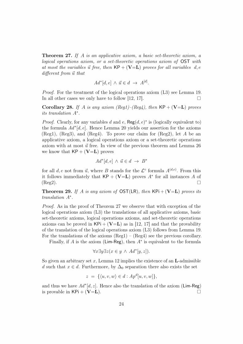
Theorem 27. If A is an applicative axiom, a basic set-theoretic axiom, alogical operations axiom, or a set-theoretic operations axiom of OST withat most the variables ~u free, then KP + (V=L) proves for all variables d, edifferent from ~u that

Ad∗[d, e] ∧ ~u ∈ d → A[d].

Proof. For the treatment of the logical operations axiom (L3) see Lemma 19.In all other cases we only have to follow [12, 17].

Corollary 28. If A is any axiom (Reg1)–(Reg4), then KP + (V=L) provesits translation A∗.

Proof. Clearly, for any variables d and e, Reg(d, e)∗ is (logically equivalent to)the formula Ad∗[d, e]. Hence Lemma 20 yields our assertion for the axioms(Reg1), (Reg3), and (Reg4). To prove our claim for (Reg2), let A be anapplicative axiom, a logical operations axiom or a set-theoretic operationsaxiom with at most ~u free. In view of the previous theorem and Lemma 26we know that KP + (V=L) proves

Ad∗[d, e] ∧ ~u ∈ d → B∗

for all d, e not from ~u, where B stands for the L◦ formula A(d,e). From thisit follows immediately that KP + (V=L) proves A∗ for all instances A of(Reg2).

Theorem 29. If A is any axiom of OST(LR), then KPi + (V=L) proves itstranslation A∗.

Proof. As in the proof of Theorem 27 we observe that with exception of thelogical operations axiom (L3) the translations of all applicative axioms, basicset-theoretic axioms, logical operations axioms, and set-theoretic operationsaxioms can be proved in KPi + (V=L) as in [12, 17] and that the provabilityof the translation of the logical operations axiom (L3) follows from Lemma 19.For the translations of the axioms (Reg1) – (Reg4) see the previous corollary.

Finally, if A is the axiom (Lim-Reg), then A∗ is equivalent to the formula

∀x∃y∃z(x ∈ y ∧ Ad∗[y, z]).

So given an arbitrary set x, Lemma 12 implies the existence of an L-admissibled such that x ∈ d. Furthermore, by ∆0 separation there also exists the set

z = {〈u, v, w〉 ∈ d : Apd[u, v, w]},

and thus we have Ad∗[d, z]. Hence also the translation of the axiom (Lim-Reg)is provable in KPi + (V=L).

24

From this theorem we conclude that the system OST(LR) is interpretablein the theory KPi + (V=L). Moreover, KPi + (V=L) is conservative over KPifor formulas which are absolute with respect to KP. Together with Theorem 15we thus obtain the following final result.

Corollary 30. The two theories OST(LR) and KPi are proof-theoreticallyequivalent.

In this paper a new form of relativizing operational set theory has beenintroduced and, based on that, a natural operational set theory of the sameproof-theoretic strength as the theory KPi has been formulated and analyzed.The heart of the matter in interpretating OST(LR) into KPi is giving aninductive definition of the application relation. By restricting this applicationrelation to suitable sets we then can deal with relativized regularity.

This is just one specific application of this new way of relativizing oper-ational set theory. A uniform version of the limit axiom (Lim-Reg) will bediscussed elsewhere.

In future work various large cardinal notions will be reexamined under theperspective this new form of relativizing operational set theory, for exampleby adding power set and unbounded existential quantification.

References[1] K. J. Barwise, Admissible Sets and Structures, Perspectives in Mathe-

matical Logic, vol. 7, Springer, 1975.

[2] M.J. Beeson, Foundations of Constructive Mathematics: Metamathemat-ical Studies, Ergebnisse der Mathematik und ihrer Grenzgebiete, vol. 3/6,Springer, 1985.

[3] A. Cantini, Extending constructive operational set theory by impredicativeprinciples, Mathematical Logic Quarterly 57 (2011), no. 3, 299–322.

[4] A. Cantini and L. Crosilla, Constructive set theory with operations,Logic Colloquium 2004 (A. Andretta, K. Kearnes, and D. Zambella,eds.), Lecture Notes in Logic, vol. 29, Cambridge University Press, 2007,pp. 47–83.

[5] , Elementary constructive operational set theory, Ways of ProofTheory (R. Schindler, ed.), Ontos Mathematical Logic, vol. 2, De Gruyter,2010, pp. 199–240.

25

[6] S. Feferman, A language and axioms for explicit mathematics, Algebraand Logic (J.N. Crossley, ed.), Lecture Notes in Mathematics, vol. 450,Springer, 1975, pp. 87–139.

[7] , Notes on operational set theory, I. Generalization of “small”large cardinals in classical and admissible set theory, Technical Notes,2001.

[8] , Operational set theory and small large cardinals, Informationand Computation 207 (2009), 971–979.

[9] G. Jäger, Die konstruktible Hierarchie als Hilfsmittel zur beweistheo-retischen Untersuchung von Teilsystemen der Mengenlehre und Analysis,Ph.D. thesis, Mathematisches Institut, Universität München, 1979.

[10] , A well-ordering proof for Feferman’s theory T0, Archiv fürMathematische Logik und Grundlagenforschung 23 (1983), no. 1, 65–77.

[11] , Theories for Admissible Sets: A Unifying Approach to ProofTheory, Studies in Proof Theory, Lecture Notes, vol. 2, Bibliopolis, 1986.

[12] , On Feferman’s operational set theory OST, Annals of Pure andApplied Logic 150 (2007), no. 1–3, 19–39.

[13] , Full operational set theory with unbounded existential quantifica-tion and power set, Annals of Pure and Applied Logic 160 (2009), no. 1,33–52.

[14] , Operations, sets and classes, Logic, Methodology and Philoso-phy of Science – Proceedings of the Thirteenth International Congress(C. Glymour, W. Wei, and D. Westerståhl, eds.), College Publications,2009, pp. 74–96.

[15] , Operational closure and stability, Annals of Pure and AppliedLogic 164 (2013), no. 7–8, 813–821.

[16] G. Jäger and W. Pohlers, Eine beweistheoretische Untersuchung von(∆1

2-CA)+(BI) und verwandter Systeme, Sitzungsberichte der BayerischenAkademie der Wissenschaften, Mathematisch-NaturwissenschaftlicheKlasse 1 (1982), 1–28.

[17] G. Jäger and R. Zumbrunnen, About the strength of operational regularity,Logic, Construction, Computation (U. Berger, H. Diener, P. Schuster,and M. Seisenberger, eds.), Ontos Mathematical Logic, vol. 3, De Gruyter,2012, pp. 305–324.

26

[18] , Explicit mathematics and operational set theory: some onto-logical comparisons, The Bulletin of Symbolic Logic 20 (2014), no. 3,275–292.

[19] K. Kunen, Set Theory. An Introduction to Independence Proofs, Studiesin Logic and the Foundations of Mathematics, vol. 102, Elsevier, 1980.

[20] D. Probst, Pseudo-hierarchies in admissible set theory without founda-tion and explicit mathematics, Ph.D. thesis, Institut für Informatik undangewandte Mathematik, Universität Bern, 2005.

[21] A.S. Troelstra and D. van Dalen, Constructivism in Mathematics, I,Studies in Logic and the Foundations of Mathematics, vol. 121, Elsevier,1988.

[22] R. Zumbrunnen, Contributions to operational set theory, Ph.D. thesis,Institut für Informatik und angewandte Mathematik, Universität Bern,2013.

AddressGerhard Jäger, Institut für Informatik, Universität Bern, Neubrückstrasse 10,CH-3012 Bern, Switzerland, jaeger@inf.unibe.ch

27