Embed Size (px)
Citation preview
Reliability and efficiency of an anisotropic
Zienkiewicz-Zhu error estimator
Stefano Micheletti Simona Perotto
MOX– Modellistica e Calcolo ScientificoDipartimento di Matematica “F. Brioschi”
Politecnico di Milanovia Bonardi 9, 20133 Milano, Italy
[email protected], [email protected]
KeywordsReliability and efficiency of an error estimator, recovery-based error estimators, anisotropicmesh adaption, finite elements.
Abstract
In this paper we study the efficiency and the reliability of an anisotropic aposteriori error estimator in the case of the Poisson problem supplied with mixedboundary conditions. The error estimator may be classified as a residual-basedone, but its novelty is twofold: firstly, it employs anisotropic estimates of theinterpolation error for linear triangular finite elements and, secondly, it makes useof the Zienkiewicz-Zhu recovery procedure to approximate the gradient of the exactsolution. Finally, we describe the adaptive procedure used to obtain a numericalsolution satisfying a given accuracy, and we include some numerical test cases toassess the robustness of the proposed numerical algorithm.
1 Introduction and motivations
In [27, 31] an error estimator computationally cheap but, at the same time, able to detectthe directional features of the solution of the problem at hand is introduced. Thesegood properties are obtained by suitably combining the Zienkiewicz-Zhu (ZZ) gradientrecovery procedure [40, 41, 42, 43] with the anisotropic error estimates of [11, 12]. Thisis carried out first by developing a residual-based error estimator. Then the error inthe interpolation terms is bounded via suitable anisotropic error estimates. Finally,the derivatives of the exact solution entering these anisotropic terms are replaced byrecovered quantities, in the spirit of the ZZ procedure.
Let us show in more detail how this error estimator is obtained in a quite generalsetting. Suppose that the weak form of the problem at hand is:find u ∈ V such that, for any v ∈ V ,
B(u, v) = L(v), (1)
where V is a Hilbert space, B(·, ·) : V × V → R is a coercive symmetric bilinear form,L : V → R is an element of the dual space V ′ of V . Then the approximated problem is:find uh ∈ Vh such that, for any vh ∈ Vh,
B(uh, vh) = L(vh),
1

where Vh ⊂ V is a suitable finite dimensional subspace of V . Then it follows that, forany v ∈ V ,
B(u − uh, v) = L(v) − B(uh, v) = R(v),
R ∈ V ′ being the (weak) residual associated with (1). The well-known Galerkin orthog-onality property (R(vh) = 0, for any vh ∈ Vh), yields
B(u − uh, v) = R(v − vh).
By localizing the residual term over the elements K and the edges of the triangulationTh, and using the Cauchy-Schwarz inequality as well as suitable interpolation errorestimates, we have
|B(u − uh, v)| ≤ C∑
K∈Th
αK ρK(uh) wK(v), (2)
where αK are area-dependent coefficients, while ρK(uh) and wK(v) are the local (interiorand edge) residual terms and the anisotropic weights associated with the function v,respectively, with C a suitable constant. By identifying in (2) v with the discretizationerror eh = u − uh, we get
B(eh, eh) ≤ C∑
K∈Th
αK ρK(uh) wK(eh). (3)
We may characterize such a result as an implicit estimate for the energy norm of eh,since eh appears at both the left and right-hand sides of (3), the energy norm beingdefined by the bilinear form itself. The idea now is to replace the above term wK(eh),usually depending on the first and/or the second derivatives of eh, with the computablequantity wK(e∗h), obtained by employing, for instance, recovered derivatives of u insteadof the exact ones, following the ZZ approach. Thus the final estimator for the energynorm of eh is defined by
η =( ∑
K∈Th
η2K
)1/2
, (4)
with ηK =(αKρK(uh)wK(e∗h)
)1/2.
Since the pioneering work [40] dealing with the linear elastic problem, and some fur-ther papers [42, 43], it has been attempted to theoretically understand the amazinglygood properties of the ZZ error estimator, obtained by approximating the true gradient,for instance, with the recovered one. One of the first work in which some averaging tech-nique is studied is [20], though the idea is nearly as old as the finite element method itself(see, e.g., [39]). In the literature emphasis is often given to superconvergence results,that is, the phenomenon observed when using, for example, continuous piecewise linearfinite elements: the convergence rate of the averaged gradient to the exact gradient inthe L2-norm can locally be higher, even by one order, than that of the original piecewiseconstant discrete gradient, under some smoothness assumption on the solution and onthe domain, and under some regularity constraints on the mesh. For instance, in [20]uniform triangulations are necessary; in [21] a regular family of uniform triangulationsof a polygonal domain is considered; in [10] a quasi-parallelism assumption is made; in[24] generalizations of previous results assuming fully-structured partitions or strongly-regular meshes to globally mildly structured meshes are derived. Theoretical propertiesof different types of ZZ-like error estimators are considered also in e.g. [3, 5, 23, 37, 38].
2

Aim of this paper is to study the efficiency and the reliability of an anisotropic aposteriori error estimator of the type (4), in the case of the Poisson problem providedwith mixed boundary conditions.Some numerical tests on anisotropic error estimators of type (4) have already beenpresented in [27, 31] while generalization to other elliptic problems and to parabolicproblems are discussed in [32].
The outline of the paper is as follows: after introducing the anisotropic settingin Section 2, we derive in Section 3 the anisotropic error estimator of type (4) for amodel elliptic boundary value problem. In Section 4 we provide the theoretical tools forstudying the reliability and the efficiency of the error estimator, carried out in Section 5and 6, respectively. Finally, in Section 7 we discuss how the anisotropic error estimatorcan be used to generate an adapted mesh and we numerically validate the proposedtheory on some test cases.
2 Functional and anisotropic framework
Let us introduce the functional spaces used in the sequel. Let Ω be a polygonal domainof R
2with Lipschitz continuous boundary ∂Ω. First, let L2(Ω) be the space of the
Lebesgue square-integrable functions with norm ‖ · ‖L2(Ω) and scalar product (·, ·).Then let W k,p(Ω) be the classical Sobolev spaces of functions for which the p-th powerof their distributional derivatives of order up to k ≥ 0 is Lebesgue-measurable and1 ≤ p < ∞ [25]. In particular, for p = 2, the space W k,2(Ω) is denoted with Hk(Ω),with norm and seminorm ‖ · ‖Hk(Ω) and | · |Hk(Ω), respectively. When these norms orseminorms are referred to some subset S of Ω, they are written as ‖ · ‖L2(S), ‖ · ‖Hk(S)
and | · |Hk(S).Moreover, in the case p = 2 and k = 1 we let H1
Γ(Ω) be the subspace of functionsof H1(Ω) satisfying homogeneous Dirichlet boundary conditions on a subset Γ of theboundary ∂Ω of Ω, with Γ 6= ∅. Finally, we recall that L∞(Ω) is the space of boundedfunctions a.e. in Ω.The remaining part of this section is devoted to the introduction of the anisotropicsetting used to derive the anisotropic a posteriori error estimator in Section 3.1. Thedetails of the anisotropic analysis we are referring to are covered essentially in [11, 12].
For any 0 < h ≤ 1, let Thh be a family of conforming triangulations of Ω into tri-angles K of diameter hK ≤ h. Since we are working with strongly anisotropic meshes,the standard regularity assumption on the mesh does not hold [7]. Let us introduce
the standard invertible affine map TK : K → K from the reference triangle K to thegeneral element K of the triangulation Th (see Fig. 1). Although the results in [11, 12]
are independent of K, in the sequel, we identify K with the unitary equilateral trian-gle (−1/2, 0), (1/2, 0), (0,
√3/2). This turns out to be a practical and rather standard
choice for an anisotropic analysis [2, 9, 18, 22, 35].
3

1,K
r1,K
r2,K
K
2,K
K
K
T
λ
λ
r= 33
r
1
Figure 1: The affine map TK .
For any K ∈ Th, let MK ∈ R2×2
and ~tK ∈ R2
be the matrix and the vector defining
the map TK , that is, for any ~x = (x1, x2)T ∈ K,
~x = (x1, x2)T = TK(~x) = MK
~x + ~tK ∈ K . (5)
The anisotropic information about the size and the orientation of the mesh element Kare derived by the spectral properties of the map TK . In more detail, let us consider thepolar decomposition MK = BK ZK of the matrix MK in (5), with BK and ZK ∈ R
2×2
symmetric positive definite and orthogonal matrices, respectively (see, e.g., [17]). Thenlet us factorize the matrix BK in terms of its eigenvalues λi,K and eigenvectors ~ri,K toobtain MK = RT
K ΛK RK ZK , with RTK = [~r1,K ~r2,K ] and ΛK = diag(λ1,K , λ2,K). In
the sequel the non-restrictive assumption λ1,K ≥ λ2,K is made.
The deformation of any K ∈ Th with respect to K can thus be measured in terms ofthe quantities λi,K by defining the so-called stretching factor sK = λ1,K/λ2,K (≥ 1), s
Kbeing equal to one. Notice that the matrix BK and all the quantities related to it areindependent of the local numbering of the nodes of K only when K is the (isotropic)equilateral triangle.
In view of the a posteriori error analysis below, after introducing the finite elementspace Wh ⊂ H1(Ω) consisting of piecewise continuous polynomials of degree one, letI1h : L2(Ω) → Wh be the standard Clement linear interpolant [8], and let I1
K be itsrestriction to K, for any K ∈ Th. Throughout two requirements are made on thepatch ∆K involved in the definition of the operator I1
h, ∆K being the union of all theelements sharing a vertex with K. We assume the cardinality of any patch ∆K aswell as the diameter of the reference patch ∆
K = T−1K (∆K) to be uniformly bounded,
independently of the geometry of the mesh, i.e., for any K ∈ Th,
card(∆K) < N and diam(∆
K) ≤ C∆ ' O(1), (6)
with C∆ ≥ h
K [26]. In particular, the latter hypothesis rules out some too distortedreference patches (see Fig. 2 where examples of acceptable and non-acceptable patchesare provided).
For the Clement operator I1h the following anisotropic interpolation error estimates
can be proved [11, 12].
4

1
T
T
K
K
x
x
x
x
xx
x
1 1
11
2x2
2 2^
^
^
^
1
1
1
1H
H
H
H
HH 1
2
1
2
2
1
H
H
1
1
K
K K
K^
^
Figure 2: Examples of an acceptable (top) and of a non-acceptable (bottom) patch.
Lemma 2.1 Let v ∈ H1(Ω). Then there exist two constants C1 = C1(N, C∆) andC2 = C2(N, C∆) such that, for any K ∈ Th,
‖v − I1K(v)‖L2(K) ≤ C1
[ 2∑
i=1
λ2i,K
(~r T
i,K GK(v)~ri,K
)]1/2
,
‖v − I1K(v)‖L2(∂K) ≤ C2 h
1/2K
[sK
(~r T1,K GK(v)~r1,K
)+
1
sK
(~r T2,K GK(v)~r2,K
)]1/2
,
(7)GK(v) being the symmetric positive semi-definite matrix given by
GK(v) =∑
T∈∆K
∫
T
( ∂v
∂x1
)2
d~x
∫
T
∂v
∂x1
∂v
∂x2d~x
∫
T
∂v
∂x1
∂v
∂x2d~x
∫
T
( ∂v
∂x2
)2
d~x
. (8)
Remark 2.1 Estimates (7) hold also for a more general Clement like operator suchas, for instance, the Scott-Zhang interpolant [34]. In such a case it suffices to suitablymodify the definition of the patch ∆K in (8).
5

3 The model problem
Let us consider the model elliptic boundary value problem: find u : Ω → R such that
−2∑
i, j=1
∂
∂xi
(aij
∂u
∂xj
)+ γu = f in Ω,
u = 0 on ΓD,
∂u
∂~nL= g on ΓN ,
(9)
where ΓD and ΓN , with ΓD 6= ∅, denote two disjoint boundary segments such thatΓD ∪ ΓN = ∂Ω; f ∈ L2(Ω), g ∈ L2(ΓN ), γ = γ(~x) ≥ 0 a.e. in Ω and aij = aij(~x) =aji(~x) ∈ L∞(Ω) are given functions, and
∂u
∂~nL=
2∑
i, j=1
aij∂u
∂xjni
is the conormal derivative of u, ~n = (n1, n2)T being the unit outward normal vector to
the boundary ∂Ω of the domain Ω. Moreover, we assume that the differential operatordefined in (9) is elliptic, i.e. that there exists a constant δ > 0 such that
2∑
i, j=1
aij(~x) ξi ξj ≥ δ ‖ ~ξ ‖22
for any ~ξ = (ξ1, ξ2)T ∈ R
2and for a.e. ~x ∈ Ω, ‖ · ‖2 denoting the standard Euclidean
norm. The weak form of (9) reads: find u ∈ V ≡ H1ΓD
(Ω) such that
B(u, v) = L(v) for any v ∈ V, (10)
where
B(u, v) =
∫
Ω
( 2∑
i, j=1
aij∂u
∂xj
∂v
∂xi+ γ u v
)d~x and L(v) =
∫
Ω
f v d~x +
∫
ΓN
g v ds.
The hypotheses made above on the data of problem (9) guarantee the existence and theuniqueness of the solution u of the weak formulation (10). Let us endow the space Vwith the energy norm ||| · ||| defined by
|||v||| = [B(v, v)]1/2 for any v ∈ V. (11)
In what follows, without any explicit specification, we will refer such a norm to the wholedomain Ω. Otherwise the considered subset of Ω will be specified by a correspondingsubscript. Let us introduce the subspace Vh ⊂ V consisting of piecewise continuouspolynomials of maximum degree one [7, 33]. Then the discrete form of (10) reads: finduh ∈ Vh such that
B(uh, vh) = L(vh) for any vh ∈ Vh. (12)
Existence and uniqueness of uh are again guaranteed by the hypotheses made above onthe data of problem (9). Recalling that eh = u − uh is the discretization error associ-ated with the finite element solution uh, this quantity satisfies the so-called Galerkinorthogonality property given by
B(eh, vh) = 0 for any vh ∈ Vh. (13)
Moving from [27, 31], we are now in a position to build the desired anisotropic counter-part of the standard ZZ error estimator [40, 41, 42, 43].
6
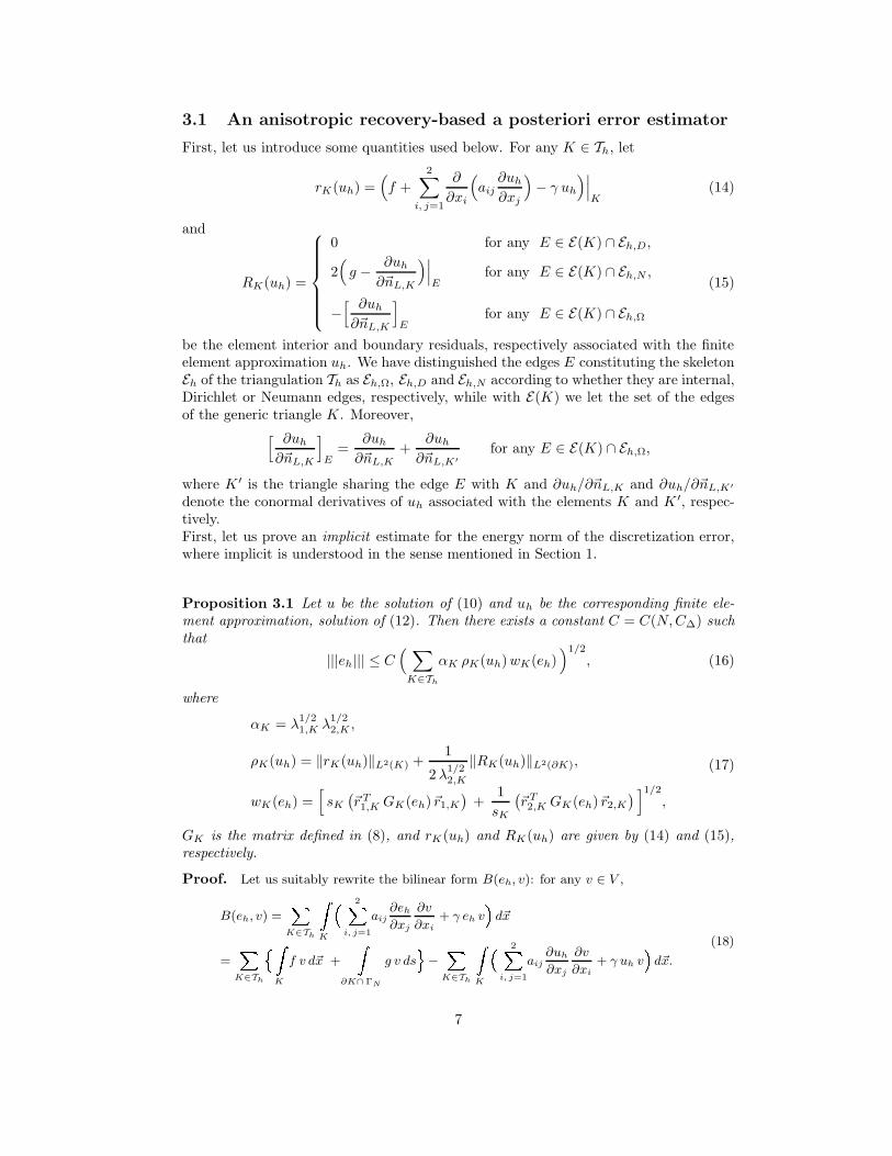
3.1 An anisotropic recovery-based a posteriori error estimator
First, let us introduce some quantities used below. For any K ∈ Th, let
rK(uh) =(f +
2∑
i, j=1
∂
∂xi
(aij
∂uh
∂xj
)− γ uh
)∣∣∣K
(14)
and
RK(uh) =
0 for any E ∈ E(K) ∩ Eh,D,
2(
g − ∂uh
∂~nL,K
)∣∣∣E
for any E ∈ E(K) ∩ Eh,N ,
−[ ∂uh
∂~nL,K
]E
for any E ∈ E(K) ∩ Eh,Ω
(15)
be the element interior and boundary residuals, respectively associated with the finiteelement approximation uh. We have distinguished the edges E constituting the skeletonEh of the triangulation Th as Eh,Ω, Eh,D and Eh,N according to whether they are internal,Dirichlet or Neumann edges, respectively, while with E(K) we let the set of the edgesof the generic triangle K. Moreover,
[ ∂uh
∂~nL,K
]E
=∂uh
∂~nL,K+
∂uh
∂~nL,K′
for any E ∈ E(K) ∩ Eh,Ω,
where K ′ is the triangle sharing the edge E with K and ∂uh/∂~nL,K and ∂uh/∂~nL,K′
denote the conormal derivatives of uh associated with the elements K and K ′, respec-tively.First, let us prove an implicit estimate for the energy norm of the discretization error,where implicit is understood in the sense mentioned in Section 1.
Proposition 3.1 Let u be the solution of (10) and uh be the corresponding finite ele-ment approximation, solution of (12). Then there exists a constant C = C(N, C∆) suchthat
|||eh||| ≤ C( ∑
K∈Th
αK ρK(uh) wK(eh))1/2
, (16)
where
αK = λ1/21,K λ
1/22,K ,
ρK(uh) = ‖rK(uh)‖L2(K) +1
2 λ1/22,K
‖RK(uh)‖L2(∂K),
wK(eh) =[sK
(~r T1,K GK(eh)~r1,K
)+
1
sK
(~r T2,K GK(eh)~r2,K
) ]1/2
,
(17)
GK is the matrix defined in (8), and rK(uh) and RK(uh) are given by (14) and (15),respectively.
Proof. Let us suitably rewrite the bilinear form B(eh, v): for any v ∈ V ,
B(eh, v) =
K∈Th
K
2i, j=1
aij∂eh
∂xj
∂v
∂xi+ γ eh v d~x
=
K∈Th K
f v d~x +
∂K∩ΓN
g v ds −
K∈Th
K
2i, j=1
aij∂uh
∂xj
∂v
∂xi+ γ uh v d~x.
(18)
7

An integration by parts of the integral in the last sum yields
−
K∈Th
K
2i, j=1
aij∂uh
∂xj
∂v
∂xi+ γ uh v d~x =
K∈Th
K
2i, j=1
∂
∂xi aij∂uh
∂xj
− γ uh v d~x −
∂K∩ΓN
∂uh
∂~nL,Kv ds −
∂K∩Eh,Ω
∂uh
∂~nL,Kv ds .
Thus, going back to (18) and thanks to (14) and (15), we get
B(eh, v) =
K∈Th K f +
2i, j=1
∂
∂xi aij∂uh
∂xj − γ uh v d~x
+
∂K∩ΓN g − ∂uh
∂~nL,K v ds −
∂K∩Eh,Ω
∂uh
∂~nL,Kv ds
=
K∈Th K
rK(uh) v d~x +1
2
∂K
RK(uh) v ds .
Now the Galerkin orthogonality property (13) (with vh = I1h(v)) together with the Cauchy-
Schwarz inequality and Lemma 2.1 provide the estimate
|B(eh, v)| = B eh, v − I1
h(v) ≤ K∈Th ‖rK(uh)‖L2(K) ‖v − I1
K(v)‖L2(K)
+1
2‖RK(uh)‖L2(∂K) ‖v − I1
K(v) ‖L2(∂K) ≤ C
K∈Th ‖rK(uh)‖L2(K) 2
i=1
λ2i,K
~r T
i,K GK(v)~ri,K 1/2
+h
1/2K
2‖RK(uh)‖L2(∂K) sK
~r T1,K GK(v)~r1,K +
1
sK
~r T2,K GK(v)~r2,K 1/2
≤ C
K∈Th λ1/21,K λ
1/22,K‖rK(uh)‖L2(K) +
λ1/21,K
2‖RK(uh)‖L2(∂K)
sK
~r T1,K GK(v)~r1,K +
1
sK
~r T2,K GK(v)~r2,K 1/2 ,
i.e. result (16) after choosing v = eh. Notice that in the last inequality the geometrical relation
hE ≤ hK ≤ h Kλ1,K , for any K ∈ Th, (19)
has been exploited also. To get information from estimate (16), we replace the matrix GK(eh) in the definition ofthe weights wK(eh) with a computable quantity, eh depending on the unknown solutionu. With this aim, we exploit the ZZ recovery technique and replace GK(eh) with thenew matrix GK(e∗h) defined by
(GK(e∗h))ij =∑
T∈∆K
∫
T
(Giuh − ∂uh
∂xi
)(Gjuh − ∂uh
∂xj
)d~x with i, j = 1, 2, (20)
GZZuh = (G1uh, G2uh)T ∈ (Wh)2 denoting the ZZ recovered gradient.
8

Remark 3.1 Throughout we employ the following definition of GZZuh:
GZZuh(~xi) =1
|∆i|∑
T∈∆i
|T | ∇uh
∣∣T,
where ∆i is the patch of elements sharing the generic node ~xi, and |T |, |∆i| are themeasures of T and ∆i, respectively. This corresponds to an approximate L2-projection,where the scalar product are evaluated using the trapezoidal quadrature formula.
Matrix (20) allows us to provide the definition below.
Definition 3.1 An anisotropic a posteriori error estimator for the energy norm of thediscretization error eh associated with the finite element approximation uh of problem(10), is given by the quantity
η =( ∑
K∈Th
η2K
)1/2
, (21)
where ηK =(αK ρK(uh) wK(e∗h)
)1/2is the element error indicator. According to (17)3,
wK(e∗h) =
[sK
(~r T1,K GK(e∗h)~r1,K
)+
1
sK
(~r T2,K GK(e∗h)~r2,K
) ]1/2
, (22)
while αK and ρK(uh) are defined as in (17)1 and (17)2, respectively.
We point out that the error estimator (21) is of residual type (see, e.g., [1, 36]).However, though computationally cheap, it allows us to estimate only the energy normof the discretization error eh. If linear functionals of eh have to be controlled, dual-based error estimators, involving the solution of a suitable adjoint problem, should beconsidered [4, 16, 30]. Anisotropic error estimates for the control of linear functionalsof the discretization error are considered, for instance, in [12, 13, 14, 28].
4 Foreword to the analysis
Given a generic estimator η of the discretization error eh in the energy norm, checkingthe robustness of η means verifying its efficiency and reliability i.e. the existence of twostrictly positive constants C, C, independent of the mesh size, such that
|||eh||| ≤ C η + H.O.T.1 (reliability) (23)
andηK ≤ C |||eh|||∆K
+ H.O.T.2 (efficiency), (24)
where ηK is the element error indicator associated with η and H.O.T.i, with i = 1, 2,are higher order terms related to the data oscillations (see [29]).Essentially, relations (23) and (24) state the upper (global) and lower (local) bounded-ness of the energy norm of eh in terms of the global and of the element error indicatorsη and ηK , respectively.The reliability and the efficiency of the error estimator η in (21) are analyzed in Sections5 and 6, respectively after making some simplifying choices on the starting problem (9):the diffusive matrix A = aij is assumed constant, while the reaction term γu isneglected. Thus, the element internal residual reduces to rK(uh) = f |K because of the
9

choice of the finite element space.Then we replace the data f and g, usually not exactly integrable, by suitable functionsfK and gE, piecewise constant with respect to Th and Eh,N , respectively [29, 36]. Theelement error indicator ηK in (21) can thus be explicitly rewritten as
ηK,T =[λ
1/21,Kλ
1/22,K ‖fK‖L2(K) +
λ1/21,K
2
∑
E∈E(K)∩Eh,Ω
∥∥∥[ ∂uh
∂~nL,K
]E
∥∥∥L2(E)
+ λ1/21,K
∑
E∈E(K)∩Eh,N
∥∥∥(gE − ∂uh
∂~nL,K
)∣∣∣E
∥∥∥L2(E)
]1/2 (wK(e∗h)
)1/2,
(25)
ηK,T being now an exactly computable quantity.Finally, the reliability and the efficiency of the error indicator
ηT =( ∑
K∈Th
η2K,T
)1/2
(26)
will be studied under the additional
Assumption 4.1 For any K ∈ Th,
∥∥∥ ∂u
∂xi− Giuh
∥∥∥L2(∆K)
≤ νK
∥∥∥∂eh
∂xi
∥∥∥L2(∆K)
for i = 1, 2, (27)
with νK ’s constants such that 0 ≤ νK < 1.
Assumption 4.1 is not so unusual in the literature. It is the main idea of the ZZ recoverytechnique, i.e. that the reconstruction GZZuh of the approximation ∇uh for the gradient∇u turns out to be better than ∇uh itself. However, we remark that assumption (27)is stronger than what is usually assumed, that is ‖∇u − GZZu‖L2(Ω) ≤ ν‖∇eh‖L2(Ω),with 0 ≤ ν < 1 [6, 36].
4.1 Some useful results
Let us provide some results used in the sequel to assess the reliability and the efficiencyof the error estimator (26).
Lemma 4.1 For any function v ∈ H1(∆K) and for any α, β > 0, it holds
min(α, β) ≤α
(~r T1,K GK(v)~r1,K
)+ β
(~r T2,K GK(v)~r2,K
)
|v|2H1(∆K)
≤ max(α, β),
GK being the matrix defined in (8).
Proof. Without loss of generality, let us assume that α ≥ β. Vice versa it suffices toexchange in the following the roles played by ~r1,K and ~r2,K . As ~r1,K and ~r2,K are orthonormal(eigen)vectors, let ~r1,K = [c s]T and ~r2,K = [−s c]T , with c = cos θ, s = sin θ and θ ∈ [0, π[.
10

Let W (v) be the matrix with componentsW (v)
i,j= (∂v/∂xi) (∂v/∂xj), for i, j = 1, 2.
Then we have
α (~r T1,K W (v)~r1,K) + β (~r T
2,K W (v)~r2,K)
= α ∂v
∂x1 2
c2 + 2∂v
∂x1
∂v
∂x2s c + ∂v
∂x2 2
s2 + β ∂v
∂x1 2
s2 − 2∂v
∂x1
∂v
∂x2s c + ∂v
∂x2 2
c2 = ∂v
∂x1 2
(α c2 + β s2) + 2∂v
∂x1
∂v
∂x2(α − β) s c + ∂v
∂x2 2
(α s2 + β c2)
= ∂v
∂x1
∂v
∂x2 α c2 + β s2 (α − β)s c
(α − β)s c α s2 + β c2 ∂v
∂x1
∂v
∂x2
.
Thus we are led to bound the last term of the chain of equalities above to obtain
β ∂v
∂x1 2
+ ∂v
∂x2 2
≤ ∂v
∂x1
∂v
∂x2 α c2 + β s2 (α − β)s c
(α − β)s c α s2 + β c2 ∂v
∂x1
∂v
∂x2
≤ α ∂v
∂x1 2
+ ∂v
∂x2 2
since α and β are easily shown to be the maximum and minimum eigenvalue of the matrix
above. After integrating over ∆K the thesis follows. Analogously to Lemma 4.1, we have
Lemma 4.2 For any α, β > 0, we have
min(α, β) ≤α
(~r T1,K GK(e∗h)~r1,K
)+ β
(~r T2,K GK(e∗h)~r2,K
)
‖GZZuh −∇uh‖2L2(∆K)
≤ max(α, β), (28)
GK(e∗h) being defined as in (20).
Proof. It is enough to repeat the proof of Lemma 4.1 simply by replacing the matrix W (v)
with the matrix of components Giuh − ∂uh
∂xi Gjuh − ∂uh
∂xj .
Notice that both the upper and lower bounds in Lemmas 4.1 and 4.2 are sharp.
Let us derive now a relation between ∇eh and the corresponding “recovered” quantity(GZZuh −∇uh).
Lemma 4.3 Under the Assumption 4.1 and for any K ∈ Th, we have that
1
(1 + νK)‖GZZuh −∇uh‖L2(∆K) ≤ ‖∇eh‖L2(∆K) ≤
1
(1 − νK)‖GZZuh −∇uh‖L2(∆K).
(29)
Proof. From (27) and thanks to the triangle inequality, we deduce that, for i = 1, 2, ∂eh
∂xi
L2(∆K)
≤ νK
∂eh
∂xi
L2(∆K)
+ Giuh − ∂uh
∂xi
L2(∆K)
11

that is ∂eh
∂xi
L2(∆K)
≤ 1
1 − νK
Giuh − ∂uh
∂xi
L2(∆K)
. (30)
The upper bound in (29) immediately follows from (30). Likewise, it can be inferred that,for i = 1, 2, Giuh − ∂uh
∂xi
L2(∆K)
≤ (1 + νk) ∂eh
∂xi
L2(∆K)
i.e. ∂eh
∂xi
L2(∆K)
≥ 1
1 + νk
Giuh − ∂uh
∂xi
L2(∆K)
.
This completes the proof of (29). The next Lemma relates the L2(K)-norm of the gradient of any function v ∈ H1(K) tothe energy norm of v, on a generic triangle K.
Lemma 4.4 Let γmax and γmin denote the maximum and minimum eigenvalue of thediffusive matrix A, respectively. Then for any K ∈ Th and for any v ∈ H1(K), thefollowing equivalence can be proved
γ1/2min
‖∇v‖L2(K) ≤ |||v|||K ≤ γ1/2max
‖∇v‖L2(K). (31)
Proof. The simplifying hypotheses made at the beginning of this section reduce the definition(11) of the energy norm of v on K to
|||v|||2K = B(v, v) K =
K a11 ∂v
∂x1 2
+ 2 a12∂v
∂x1
∂v
∂x2+ a22 ∂v
∂x2 2 d~x. (32)
The integrand of (32) can be identified with the numerator of the Rayleigh quotient(∇v)T A∇v
(∇v)T ∇v . Now, as
γmin (∇v)T∇v ≤ (∇v)T A∇v ≤ γmax (∇v)T∇v,
we can integrate such relations on the triangle K to obtain
γmin ‖∇v‖2L2(K) ≤ |||v|||2K ≤ γmax ‖∇v‖2
L2(K),
i.e. (31). Remark 4.1 Result (31) can be reformulated on any patch of elements ∆K simply byextending the integration step from K to ∆K and under the assumption v ∈ H1(∆K).
The last result of this section turns out to be an essential tool in the proof of boththe efficiency and the reliability of the error estimator (26).
Lemma 4.5 Under the Assumption 4.1 it can be proved that, for any K ∈ Th,
1 − νK
s1/2K γ
1/2max
|||eh|||∆K≤ wK(e∗h) ≤ s
1/2K (1 + νK)
γ1/2min
|||eh|||∆K, (33)
γmax and γmin being defined as in Lemma 4.4.
12

Proof. First, let us exploit relation (28) by choosing α = sK and β = 1/sK . This yields
1
s1/2K
‖GZZuh −∇uh‖L2(∆K) ≤ wK(e∗h) ≤ s1/2K ‖GZZuh −∇uh‖L2(∆K).
Now, for any K ∈ Th, from (29), we have
(1 − νK)
s1/2K
‖∇eh‖L2(∆K) ≤ wK(e∗h) ≤ s1/2K (1 + νK) ‖∇eh‖L2(∆K)
which immediately provides (33) thanks to Lemma 4.4 extended to the whole patch ∆K . 4.2 Anisotropic bubble functions
Typically, the efficiency of an error estimator is studied by using the properties of bubblefunctions (see, e.g., [1, 36]).In particular, we base the efficiency analysis of Section 6 on a new type of bubblefunctions which we define anisotropic bubble functions. This turns out to be the mainnovelty of our analysis.Like in the case of the standard bubble functions, we distinguish between triangle andedge bubble functions, denoted in the sequel with bA
K and bAE , respectively. We define
both types of bubbles through the solution of suitable eigenvalue problems.For any K ∈ Th, the triangle anisotropic bubble function bA
K is defined by the relationbAK = b
K T−1K , where b
K solves the problem
−∆b
K = λ b
K in K
b
K = 0 on ∂K,(34)
∆ denoting the standard Laplacian operator. Thus bAK is determined by computing
the eigenfunction b
K in K associated with the Laplacian operator provided with ho-mogeneous Dirichlet boundary conditions, and then mapping it to triangle K via thetransformation TK . It is also understood that the eigenfunction b
K corresponds to the
least (positive) eigenvalue λ of (34) and it is normalized such that max~x∈K
bAK(~x) = 1 (see
Fig. 3, left).
−5
−4
−3
−2
−1
0
1
2
3
4
5
00.20.40.60.8
0
0.2
0.4
0.6
0.8
1
−4
−2
0
2
4
60 0.2 0.4 0.6 0.8
0
0.2
0.4
0.6
0.8
1
Figure 3: The anisotropic triangle (left) and edge (right) bubble functions bAK and bA
E
both corresponding to sK = 10.
13

Likewise for any pair of triangles K, K ′ sharing the edge E ∈ Eh,Ω, the edge bubblefunction bA
E, supported in QE = K ∪ K ′, is defined by the relations bAE
∣∣K
= b
E T−1K ,
bAE
∣∣K′
= b
E T−1K′ , where b
E solves the problem
−∆b
E = λ b
E in Q
E ,
b
E = 0 on ∂Q
E ,(35)
Q
E is the quadrilateral obtained by joining K with the equilateral triangle K ′,
(1/2, 0), (1,√
3/2), (0,√
3/2), along the side E with extremes (0,√
3/2), (1/2, 0), and
TK′ is the map from triangle K ′ to K ′.Notice that the choice made for E is not restrictive, any other edge of K will do,because of its symmetry. Moreover, since K ′ coincides with K up to a rigid motion, TK′
is characterized by the same eigenvalues λ1, K′ , λ2, K′ as the ones obtained by mapping
K directly to K ′ via the mapping TK′ . Finally, TK′ and TK coincide on E.As above, it is understood that the eigenfunction b
E corresponds to the least (positive)
eigenvalue λ of (35) and it is normalized such that max~x∈QE
bAE(~x) = 1 (see Fig. 3, right).
Results corresponding to those stated for the standard bubble functions (see, e.g.,[36]) can be proved also for bA
K and bAE . Let us summarize these properties in the
following
Lemma 4.6 For any K ∈ Th, E ∈ Eh,Ω and QE = K ∪ K ′, with K and K ′ trianglessharing the edge E, the following properties hold:
supp (bAK) ⊂ K, 0 ≤ bA
K(~x) ≤ 1 for any ~x ∈ K, max~x∈K
bAK(~x) = 1, (36)
supp (bAE) ⊂ QE , 0 ≤ bA
E(~x) ≤ 1 for any ~x ∈ QE , max~x∈E
bAE(~x) = 1, (37)
∫
K
bAK d~x = C
K |K|, (38)
∫
E
bAE ds = C∗
KhE , (39)
∫
T
bAE d~x ≤ C sT h2
E with T ∈ K, K ′, (40)
‖∇bAK‖L2(K) =
λ1/2 (1 + s2K)1/2
21/2 λ1,K‖bA
K‖L2(K) , (41)
‖∇bAE‖L2(T ) ≤
λ1/2 sT
λ1,T‖bA
E‖L2(T ) with T ∈ K, K ′, (42)
where C
K , C∗
K, C are constants depending only on the reference triangle K and sT is
the stretching factor of the element T .
Proof. Let us start with the properties of the triangle bubble function bAK . Relations (36)
follow immediately by the definition of bAK and by the choice made for its normalization.
14

Let us now prove (38). Employing the relation |K| = λ1,Kλ2,K | K|, we haveK
bAK d~x = λ1,Kλ2,K
K b K d~x =
|K|| K|
K b K d~x.
Thus, K
bAK d~x = C K |K|,
where C K =
K b K d~x/| K| depends on the reference triangle only.
To prove (41), the weak form of (34) immediately yields
‖∇b K‖2L2( K)
= λ ‖b K‖2L2( K)
.
When passing to triangle K this relation becomes
sK
~r T1,KGK(bA
K)~r1,K +1
sK
~r T2,KGK(bA
K)~r2,K =λ
λ1,Kλ2,K‖bA
K‖2L2(K), (43)
where the summation implied by the definition of the matrix GK runs only on K sincesupp(bA
K) ⊂ K. We first show that
sK
~r T1,KGK(bA
K)~r1,K =1
sK
~r T2,KGK(bA
K)~r2,K . (44)
The argument combines a slight modification of the proof of Lemma 2.2 in [11] with a symmetryargument. Let us introduce a unit vector ~χ. We express the directional derivative alongdirection ~χ of a generic function v ∈ H1( K), in terms of the derivatives of its image v definedin K. We have,
∇ v · ~χ = ~χ T MTK∇v = ~χ T ZT
KBK∇v = ~χ T ZTKRT
KΛKRK∇v .
It then follows| ∇ v · ~χ|2 = |(RKZK ~χ)T ΛKRK∇v|2 .
Choosing ~χ = ~χ1 such that RKZK ~χ1 = (1, 0)T , we obtainK| ∇ v · ~χ1|2 d~x =
K
λ21,K(~r T
1,K∇v)2 d~x
=
K
λ1,K
λ2,K(~r T
1,K∇v)2 d~x = sK
~r T1,KGK(v)~r1,K , (45)
while picking ~χ = ~χ2 such that RKZK ~χ2 = (0, 1)T , we haveK| ∇ v · ~χ2|2 d~x =
K
λ22,K(~r T
2,K∇v)2 d~x
=
K
λ2,K
λ1,K(~r T
2,K∇v)2 d~x =1
sK
~r T2,KGK(v)~r2,K .
(46)
Notice that, by construction, ~χ1 · ~χ2 = 0. Identifying in (45) and (46) v with bAK , we infer that
terms at the left and right-hand sides in (44) can be rewritten, with respect to the orthogonaldirections ~χ1 and ~χ2, as
sK
~r1,KGK(bA
K)~r1,K =
K | ∇b K · ~χ1|2 d~x ,
1
sK
~r T2,KGK(bA
K)~r2,K =
K | ∇b K · ~χ2|2 d~x ,
15

respectively. Finally, relation (44) follows on noticing that b K is invariant by rotations, thusimplying that the two integral above are equal. Property (44) together with the relation
~r T1,KGK(bA
K)~r1,K + ~r T2,KGK(bA
K)~r2,K = ‖∇bAK‖2
L2(K)
and (43), allow us to conclude
‖∇bAK‖2
L2(K) =λ(1 + s2
K)
2sKλ1,Kλ2,K‖bA
K‖2L2(K) =
λ(1 + s2K)
2λ21,K
‖bAK‖2
L2(K) ,
that is (41).Let us now deal with the properties associated with the edge bubble function bA
E . Relations(37) follow immediately from the definition and normalization of bA
E , and observing that, also
by a symmetry argument, the maximum of b E is assumed at the midpoint of E, which impliesthat the maximum of bA
E is taken at the midpoint of E as well.Equality (39) follows from
E
bAE ds =
hE
h EE b E ds = C∗KhE ,
the constant C∗K being defined as C∗K = h−1EE b E ds.
Let us now prove (40) by choosing T = K. We haveK
bAE d~x = λ1,Kλ2,K
K b E d~x = C E λ1,Kλ2,K
h2E
h2E ≤ CsKh2
E ,
where C E =
K b E d~x and having also used the relation
1
hE≤ 1
ρK≤ 1
ρ Kλ2,K, (47)
ρK , ρ K being the diameters of the balls inscribed in K and K, respectively. Thus, C = C E/ρ2K .Likewise an analogous relation holds when T = K ′.
Finally, by the invariance of the domain Q E and of the operator ∆ in (35) with respect to
a rotation of an angle π, it follows that ∂b E/∂~n E = 0, where ~n E is the unit normal across E.
This property allows us to rewrite (35) in each of the two triangles K, K′
−∆b E = λb E in K
∂b E∂~n E = 0 on E
b E = 0 on ∂ K \ E
(48)
and similarly in K′. We are now in the same position as in the case of b K as the weak form of(48) gives
‖∇b E‖2L2( K)
= λ‖b E‖2L2( K)
.
Thus a property analogous to (43) holds also for bAE|K and bA
E |K′ , where it is understood thatthe summation implied by the definition of the matrices GK and GK′ runs only on K and K ′,respectively. However, it is no longer possible to prove the analogue to (44) using the same
argument, as b E| K is not invariant by rotations in K. On the other hand, applying Lemma 4.1on K with v = bA
E|K , α = sK and β = 1/sK (and similarly on K ′), we obtain
sK
~r T1,KGK(bA
E K)~r1,K +1
sK
~r T2,KGK(bA
E K)~r2,K ≥ 1
sK‖∇bA
E‖2L2(K),
16

and then, from the analogue to (43) for bAE,
||∇bAE ||2L2(K) ≤
λλ2
2,K
||bAE ||2L2(K) =
λs2K
λ21,K
||bAE ||2L2(K),
which proves (42). Notice that (42) is less sharp than (41), the latter being and equality andbecause
1 + s2K
2 1/2
≤ sK ,
for any sK ≥ 1, with equality holding only when sK = 1. Remark 4.2 The definition provided for the edge bubble function bA
E via the problem(35) is not suited when E ∈ Eh,N . In such a case the boundary problem (35) has to bereplaced by a new one similar to (48).
We are now in a position to study the reliability and the efficiency of the errorestimator (26).
5 Reliability of ηT
Let us first prove the following Lemma, which, basically, establishes an equivalencebetween the quantities wK(eh) and wK(e∗h) provided that the stretching factor sK isbounded from above by a quantity depending on νK and such that the smaller νK , thelarger sK can be. On the contrary, should this bound not hold, then the constants inthe equivalence relations would depend on sK .
Lemma 5.1 Under the assumption that
νK(2 + νK)(1 +
s2K + 1/s2
K
2
)≤ C∗,
for some positive constant C∗ < 1/2, where νK is defined via (27), then it holds that
C1 w2K(e∗h) ≤ w2
K(eh) ≤ C2 w2K(e∗h), (49)
where C1 = C1(C∗) > 0, C2 = C2(C∗) > C1 and limνK→0
C1 = limνK→0
C2 = 1.
Proof. Let us rewrite the expression for wK(eh) and wK(e∗h) given by (17) and (22),respectively. Let ~r1,K = [c s]T and ~r2,K = [−s c]T , with c = cos θ and s = sin θ, for some
θ ∈ [0, π[. We have w2K(eh) = ~r T
1,K M ~r1,K , w2K(e∗h) = ~r T
1,K M ~r1,K where M = mij andM = mij ∈ R2×2
are the symmetric positive definite matrices given by
mij =
sK
∂eh
∂x1
2L2(∆K)
+1
sK
∂eh
∂x2
2L2(∆K)
, i = j = 1,sK − 1
sK ∆K
∂eh
∂x1
∂eh
∂x2d~x, i 6= j,
sK
∂eh
∂x2
2L2(∆K)
+1
sK
∂eh
∂x1
2L2(∆K)
, i = j = 2,
17

and
mij =
sK
G1uh − ∂uh
∂x1
2L2(∆K)
+1
sK
G2uh − ∂uh
∂x2
2L2(∆K)
, i = j = 1,
sK − 1
sK
∆K G1uh − ∂uh
∂x1 G2uh − ∂uh
∂x2 d~x, i 6= j,
sK
G2uh − ∂uh
∂x2
2L2(∆K)
+1
sK
G1uh − ∂uh
∂x1
2L2(∆K)
, i = j = 2,
respectively. To prove (49) it suffices to show under what conditions
w2K(e∗h)
w2K(eh)
=~r T1,K M ~r1,K
~r T1,K M ~r1,K
is bounded from below and from above, independently of sK . This is equivalent to requiringthat the eigenvalues µ of the generalized eigenvalue problemM~x = µM~x,
or alternatively, that the eigenvalues of the symmetric part of the positive definite matrixM−1 M do not depend on sK .
For ease of notation, throughout we let eij =
∆K
∂eh
∂xi
∂eh
∂xjd~x and Eij =
∆K
Giuh −
∂uh
∂xi Gjuh − ∂uh
∂xj d~x, for i, j = 1, 2, and for generality we let sK and 1/sK be replaced by
any two positive constants α, β, respectively, with α ≥ β.Let us rewrite the elements of M as mij = mij + εij , for i, j = 1, 2, with
εij =
α G1uh − ∂u
∂x1
2L2(∆K)
+ 2
∆K
∂eh
∂x1 G1uh − ∂u
∂x1 d~x
+ β G2uh − ∂u
∂x2
2L2(∆K)
+ 2
∆K
∂eh
∂x2 G2uh − ∂u
∂x2 d~x , i = j = 1,
(α − β) ∆K
∂eh
∂x1 G2uh − ∂u
∂x2 d~x +
∆K
∂eh
∂x2 G1uh − ∂u
∂x1 d~x
+
∆K G1uh − ∂u
∂x1 G2uh − ∂u
∂x2 d~x , i 6= j,
α G2uh − ∂u
∂x2
2L2(∆K)
+ 2
∆K
∂eh
∂x2 G2uh − ∂u
∂x2 d~x
+ β G1uh − ∂u
∂x1
2L2(∆K)
+ 2
∆K
∂eh
∂x1 G1uh − ∂u
∂x1 d~x , i = j = 2.
The “perturbations” εij can be bounded using (27) and the Cauchy-Schwarz inequality as
−2νK αe11 + βe22 ≤ ε11 ≤ νK(νK + 2) αe11 + βe22 ,
−νK(νK + 2)(α − β)e1/211 e
1/222 ≤ ε12 ≤ νK(νK + 2)(α − β)e
1/211 e
1/222 ,
−2νK αe22 + βe11 ≤ ε22 ≤ νK(νK + 2) αe22 + βe11 .
(50)
A simple computation shows that
M−1 M = I +1
det(M) m22ε11 − m12ε12 m22ε12 − m12ε22
m11ε12 − m12ε11 m11ε22 − m12ε12
,
18

where I is the identity matrix and det(M) is the determinant of M . The symmetric part of
M−1 M is thus given by (M−1 M)sym = I +1
det(M)C, with
C = cij = m22ε11 − m12ε12(m11 + m22)ε12 − m12(ε11+ε22)
2
(m11 + m22)ε12 − m12(ε11+ε22)
2m11ε22 − m12ε12
.
We next bound the entries of C by exploiting inequalities (50). Tedious but straightforwardcomputations yield
−ν2K(α − β)2e11e22 − 2νK 2(α2 + β2)e11e22 + αβ(e11 − e22)
2 ≤ c11, c22
≤ νk(νK + 2) 2(α2 + β2)e11e22 + αβ(e11 − e22)2 ,
|c12| ≤ νK(νK + 2)(α2 − β2)e1/211 e
1/222 (e11 + e22).
(51)
Moreover, using the Cauchy-Schwarz inequality
det(M) = m11m22 − m212 = (αe11 + βe22)(αe22 + βe11) − (α − β)2e2
12
≥ (αe11 + βe22)(αe22 + βe11) − (α − β)2e11e22 = αβ(e11 + e22)2.
It can be checked that the largest bound of the absolute value for c11, c22 in (51) is the upperbound, so that we obtain
|c11|m11m22 − m2
12
≤ νK(νK + 2)
2(α2 + β2)e11e22 + αβ(e11 − e22)
2 αβ(e11 + e22)2
= νK(νK + 2) e11 − e22
e11 + e22 2 a1
+2α2 + β2
αβ
e1/211 e
1/222
e11 + e22 2 a2
≤ νK(νK + 2) 1 +
α2 + β2
2αβ ,
(52)
as a1 ≤ 1 and a2 ≤ 1/4. Analogously, we have
|c12|m11m22 − m2
12
≤ νK(νK + 2)α2 − β2
αβ
e1/211 e
1/222 (e11 + e22)
(e11 + e22)2
≤ νK(νK + 2)α2 − β2
αβ
e1/211 e
1/222
e11 + e22 √
a2
≤ νK(νK + 2)α2 − β2
2αβ,
(53)
as√
a2 ≤ 1/2. The thesis follows using Gershgorin theorem to bound the eigenvalues of
(M−1 M)sym, on noting that the term 1 + (α2 + β2)/(2αβ) in (52) is always greater than
(α2−β2)/(2αβ) in (53), and recalling that, for the case at hand, α = sK , and β = 1/sK . Thus,
both the radius and the center of the two circles containing the eigenvalues of (M−1 M)sym − I
are bounded by the same quantity, i.e. the right-hand side of (52), so that the constraint
C∗ < 1/2 guarantees that the lower bound for the estimate of the eigenvalues of the matrix is
positive. We note that, while the true eigenvalues of the matrix M−1 M are positive, this may
not be the case for their estimates, unless the requirement C∗ < 1/2 is made. Moreover, as
νK → 0, both C1 and C2 tend to one, since M−1 M → I, due to (50). The reliability of the error estimator ηT in (26) is stated by the following
19
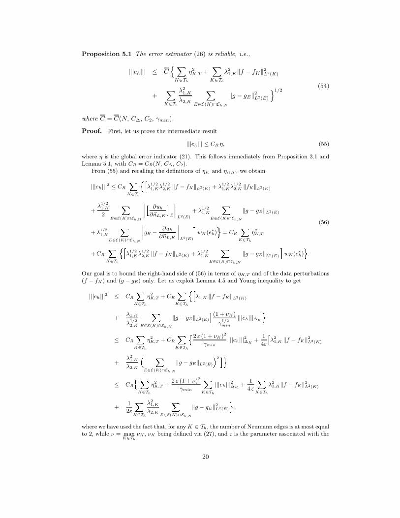
Proposition 5.1 The error estimator (26) is reliable, i.e.,
|||eh||| ≤ C ∑
K∈Th
η2K,T +
∑
K∈Th
λ21,K‖f − fK‖2
L2(K)
+∑
K∈Th
λ21,K
λ2,K
∑
E∈E(K)∩Eh,N
‖g − gE‖2L2(E)
1/2(54)
where C = C(N, C∆, C2, γmin).
Proof. First, let us prove the intermediate result
|||eh||| ≤ CR η, (55)
where η is the global error indicator (21). This follows immediately from Proposition 3.1 andLemma 5.1, with CR = CR(N, C∆, C2).
From (55) and recalling the definitions of ηK and ηK,T , we obtain
|||eh|||2 ≤ CR
K∈Th λ1/2
1,Kλ1/22,K ‖f − fK‖L2(K) + λ
1/21,Kλ
1/22,K ‖fK‖L2(K)
+λ
1/21,K
2
E∈E(K)∩Eh,Ω
∂uh
∂~nL,K
E
L2(E)
+ λ1/21,K
E∈E(K)∩Eh,N
‖g − gE‖L2(E)
+ λ1/21,K
E∈E(K)∩Eh,N
gE − ∂uh
∂~nL,K
L2(E)
wK(e∗h) = CR
K∈Th
η2K,T
+ CR
K∈Th λ1/2
1,Kλ1/22,K ‖f − fK‖L2(K) + λ
1/21,K
E∈E(K)∩Eh,N
‖g − gE‖L2(E) wK(e∗h) .
(56)
Our goal is to bound the right-hand side of (56) in terms of ηK,T and of the data perturbations(f − fK) and (g − gE) only. Let us exploit Lemma 4.5 and Young inequality to get
|||eh|||2 ≤ CR
K∈Th
η2K,T + CR
K∈Th λ1,K ‖f − fK‖L2(K)
+λ1,K
λ1/22,K
E∈E(K)∩Eh,N
‖g − gE‖L2(E) (1 + νK)
γ1/2min
|||eh|||∆K
≤ CR
K∈Th
η2K,T + CR
K∈Th 2 ε (1 + νK)2
γmin|||eh|||2∆K
+1
4ε λ21,K ‖f − fK‖2
L2(K)
+λ2
1,K
λ2,K
E∈E(K)∩Eh,N
‖g − gE‖L2(E) 2 ≤ CR
K∈Th
η2K,T +
2 ε (1 + ν)2
γmin
K∈Th
|||eh|||2∆K+
1
4 ε
K∈Th
λ21,K‖f − fK‖2
L2(K)
+1
2ε
K∈Th
λ21,K
λ2,K
E∈E(K)∩Eh,N
‖g − gE‖2L2(E) ,
where we have used the fact that, for any K ∈ Th, the number of Neumann edges is at most equalto 2, while ν = max
K∈Th
νK , νK being defined via (27), and ε is the parameter associated with the
20

Young inequality, to be suitably chosen. As from (6) it follows that
K∈Th
|||eh|||2∆K≤ N |||eh|||2,
we get
1 − 2CRεN(1 + ν)2
γmin |||eh|||2 ≤ CR
K∈Th
η2K,T
+1
4ε
K∈Th
λ21,K‖f − fK‖2
L2(K) +1
2 ε
K∈Th
λ21,K
λ2,K
E∈E(K)∩Eh,N
‖g − gE‖2L2(E) .
(57)
To make inequality (57) meaningful, we have to assure that
1 − 2CRεN(1 + ν)2
γmin> 0 i.e. ε <
γmin
2CRN(1 + ν)2.
For instance, the choice ε = γmin/(4CRN(1 + ν)2) guarantees that
|||eh||| ≤ CR
K∈Th
η2K,T +
CRN(1 + ν)2
γmin
K∈Th
λ21,K‖f − fK‖2
L2(K)
+2CRN(1 + ν)2
γmin
K∈Th
λ21,K
λ2,K
E∈E(K)∩Eh,N
‖g − gE‖2L2(E) 1/2
,
namely the reliability result (54), where C = CR max 1,8N
γminCR , with CR defined through
(55). Remark 5.1 Notice that the contribution of the data oscillation increases as N getslarger, i.e., when the maximum number of elements of a patch increases. Moreover, thereliability result does not depend explicitly on ν since this quantity appears in the form1 + ν which is uniformly bounded between 1 and 2.
6 Efficiency of ηT
To prove the efficiency of the error estimator defined in (26), let us study separately thethree terms at the right-hand side of (25):
η2K,T = λ
1/21,K λ
1/22,K‖fK‖L2(K) wK(e∗h)
︸ ︷︷ ︸( I )
+λ
1/21,K
2
( ∑
E∈E(K)∩Eh,Ω
∥∥∥[ ∂uh
∂~nL,K
]E
∥∥∥L2(E)
)wK(e∗h)
︸ ︷︷ ︸( II )
+ λ1/21,K
( ∑
E∈E(K)∩Eh,N
∥∥∥(gE − ∂uh
∂~nL,K
)∣∣∣E
∥∥∥L2(E)
)wK(e∗h)
︸ ︷︷ ︸( III )
.
(58)
In the Lemmas below we bound the three quantities ( I ), ( II ) and ( III ) in terms ofthe data perturbations (f − fK) and (g − gE), and of the energy norm |||eh|||∆K
of thediscretization error on the patch ∆K .
21

First, let us provide two results used in the sequel. The first one is relation (18)rewritten on the whole domain Ω and by recalling the simplifying assumptions made inSection 4 on the initial problem (9). We have
∫
Ω
( 2∑
i,j=1
aij∂eh
∂xj
∂v
∂xi
)d~x =
∫
Ω
fv d~x +
∫
ΓN
gv ds −∫
Ω
( 2∑
i,j=1
aij∂uh
∂xj
∂v
∂xi
)d~x. (59)
The second result is obtained by suitably integrating by parts the right-hand side of(59):
∫
Ω
fv d~x +
∫
ΓN
gv ds −∫
Ω
( 2∑
i,j=1
aij∂uh
∂xj
∂v
∂xi
)d~x
=
∫
Ω
fv d~x +
∫
ΓN
gv ds +∑
K∈Th
∫
K
( 2∑
i,j=1
aij∂2uh
∂xi ∂xjv)
d~x −∫
∂K
∂uh
∂~nL,Kv ds
=∑
K∈Th
∫
K
fv d~x +∑
E∈Eh,N
∫
E
(g − ∂uh
∂~nL,K
)v ds −
∑
E∈Eh,Ω
∫
E
[ ∂uh
∂~nL,K
]E
v ds,
(60)
the diffusive matrix A having been assumed constant.Let us begin to analyze the term ( I ) in (58).
Lemma 6.1 Under the Assumption 4.1, the bound
( I ) ≤ 1 + νK
C1/2
Kγmin
[(CA λ1/2 (1 + s2K)1/2
21/2+
γmin
4
)|||eh|||2∆K
+λ21,K ‖f −fK ||2L2(K)
](61)
holds, where γmin is the minimum eigenvalue of the constant diffusive matrix A, λ isthe eigenvalue of the problem (34), CA = 4 max
i,j=1, 2|aij |, and νK and C
K are defined by
relations (27) and (38), respectively.
Proof. First, let us introduce the auxiliary function σK defined by
σK = sign(fK) bAK |K|−1/2,
sign denoting the sign-function and where bAK is the triangle anisotropic bubble function intro-
duced in Section 4.2. Lemma 4.6 immediately yieldsK
fK σK d~x = |fK | |K|−1/2
K
bAK d~x = C K ‖fK‖L2(K),
that is
‖fK‖L2(K) =1
C KK
fK σK d~x. (62)
22

Now, since supp(σK) ⊂ K, and from equations (60), (59) and Lemma 4.6 we getK
fK σK d~x =
K
f σK d~x +
K
(fK − f) σK d~x
=
Ω
f σK d~x +
ΓN
g σK ds −Ω
2i,j=1
aij∂uh
∂xj
∂σK
∂xi d~x +
K
(fK − f) σK d~x
=
K
2i,j=1
aij∂eh
∂xj
∂σK
∂xi d~x +
K
(fK − f) σK d~x
≤ CA ‖∇eh‖L2(K)‖∇σK‖L2(K) + ‖f − fK‖L2(K)‖σK‖L2(K)
≤ |K|−1/2 K
bAK d~x 1/2
CAλ1/2 (1 + s2
K)1/2
21/2 λ1,K‖∇eh‖L2(K) + ‖f − fK‖L2(K)
= C1/2K CA
λ1/2 (1 + s2K)1/2
21/2 λ1,K‖∇eh‖L2(K) + ‖f − fK‖L2(K) .
(63)
Going back to the term ( I ) in (58) we have
( I ) ≤ λ1/21,Kλ
1/22,K
1
C1/2K CA
λ1/2 (1 + s2K)1/2
21/2 λ1,K‖∇eh‖L2(K) + ‖f − fK‖L2(K) wK(e∗h)
≤ λ1,K1
C1/2K CA
γ1/2min
λ1/2 (1 + s2K)1/2
21/2 λ1,K|||eh|||K + ‖f − fK‖L2(K) 1 + νK
γ1/2min
|||eh|||∆K
≤ 1 + νK
(C K γmin)1/2 CA
γ1/2min
λ1/2 (1 + s2K)1/2
21/2|||eh|||2∆K
+ λ1,K ‖f − fK‖L2(K)|||eh|||∆K
,
(64)where relations (62), (63), (31) and (33) have been exploited. Let us further rewrite the productλ1,K ‖f − fK‖L2(K) |||eh|||∆K
via the Young inequality:
λ1,K ‖f − fK‖L2(K) |||eh|||∆K≤ λ2
1,K
γ1/2min
‖f − fK‖2L2(K) +
γ1/2min
4|||eh|||2∆K
,
which, inserted into (64), provides the estimate (61). The term ( II ) in (58) can be bounded thanks to a similar procedure.
Lemma 6.2 Under the Assumption 4.1 it can be proved that
( II ) ≤ 3 C∗(1 + νK)
2 C∗
Kγmin
[sK
(γmin
4h
1/2
K+
CA
ρ1/2
K
)|||eh|||2∆K
+λ21,K N h
1/2
K
∑
T∈∆K
‖f − fT ‖2L2(T )
],
(65)
where
C∗
= C1/2 max(s1/2K , s
1/2K′ ) max
1 +
1
C1/2
K
, max(sK , sK′) h
K
(λ1/2 +
( 2 λ
C
K
)1/2),
K ′ is the triangle sharing edge E with K, νK , CA, γmin, C
K and λ are defined as in
Lemma 6.1, λ is the eigenvalue of the problem (35), the constants N , C∗
Kand C are
23

defined by relations (6), (39) and (40), and h
K , ρ
K are the diameter of K and of theball inscribed in it, respectively.
Proof. Let us introduce the auxiliary function σE associated with a generic internal edgeE ∈ E(K) ∩ Eh,Ω,
σE = sign ∂uh
∂~nL,K
E h
−1/2E bA
E ,
bAE denoting the edge anisotropic bubble function defined in Section 4.2. As, thanks to Lemma
4.6, E
∂uh
∂~nL,K
EσE ds = ∂uh
∂~nL,K
E
h−1/2E
E
bAE ds = C∗K ∂uh
∂~nL,K
E
L2(E)
,
we immediately deduce that ∂uh
∂~nL,K
E
L2(E)
=1
C∗KE
∂uh
∂~nL,K
EσE ds. (66)
As supp(σE) ⊂ QE , and thanks to results (60), (59) and Lemma 4.6 we inferE
∂uh
∂~nL,K
EσE ds
=
T∈QE
T
f σE d~x −Ω
f σE d~x −
ΓN
g σE ds +
Ω
2i,j=1
aij∂uh
∂xj
∂σE
∂xi d~x
=
T∈QE
T
f σE d~x −
QE 2
i,j=1
aij∂eh
∂xj
∂σE
∂xi d~x
≤ ‖f‖L2(QE) ‖σE‖L2(QE) + CA ‖∇eh‖L2(QE) ‖∇σE‖L2(QE)
≤ h−1/2E
QE
bAE d~x 1/2
‖f‖L2(QE)
+CA h K λ1/2 h−1E max(sK , sK′ ) ‖∇eh‖L2(QE)
≤ C1/2 max(s1/2K , s
1/2
K′ ) h1/2E ‖f‖L2(QE)
+CA h K h−1/2E λ1/2 max(sK , sK′ )‖∇eh‖L2(QE)
≤ C1/2 max(s1/2K , s
1/2K′ ) h
1/2E
T∈QE
‖f − fT ‖L2(T )
+h1/2E
T∈QE
‖fT ‖L2(T ) + CA h K h−1/2E λ1/2 max(sK , sK′ )‖∇eh‖L2(QE) ,
where relation (19) has been exploited. Now, by suitably using equalities (62) and (63) toestimate the norms ‖fT ‖L2(T ), we get
E
∂uh
∂~nL,K
EσE ds ≤ C
∗ h1/2E
T∈QE
‖f − fT ‖L2(T ) +CA
(ρ Kλ2,K)1/2‖∇eh‖L2(QE) ,
where relation (19), (47), together withT∈QE
‖∇eh‖L2(T ) ≤√
2 ‖∇eh‖L2(QE),
24
andh
1/2E (1 + s2
T )1/2
21/2 λ1,T≤ h
1/2E sT
h KhE
= h−1/2E h K sT ,
have been used. Thanks to the relations (31), (33) and (66), we get
( II ) ≤λ
1/21,K C
∗
2 C∗K
E∈E(K)∩Eh,Ω
h1/2E
T∈QE
‖f − fT ‖L2(T )
+CA
(γmin ρ K λ2,K)1/2|||eh|||QE
wK(e∗h)
≤ 3 C∗
2 C∗K λ1,K h1/2K
T∈∆K
‖f − fT ‖L2(T ) + CA sK
ρ K γmin 1/2
|||eh|||∆K
s1/2K (1 + νK)
γ1/2min
|||eh|||∆K
=3 C
∗(1 + νK)
2 C∗K γ1/2min
λ3/21,K
λ1/22,K
h1/2K |||eh|||∆K
T∈∆K
‖f − fT ‖L2(T )
+sK
(ρ K γmin)1/2CA |||eh|||2∆K
,
where relation
E∈E(K)∩Eh,Ω
QE ⊆ ∆K ,
along with (19), and the fact that E(K) consists of three edges have been used. Finally, weexploit the Young inequality to split the term
|||eh|||∆K
T∈∆K
‖f − fT ‖L2(T ):
λ3/21,K
λ1/22,K
|||eh|||∆K
T∈∆K
‖f − fT ‖L2(T ) ≤γ
1/2min
4sK |||eh|||2∆K
+λ2
1,K
γ1/2min
N
T∈∆K
‖f − fT ‖2L2(T ).
This yields result (65). Finally, let us consider the term ( III ) in (58).
Lemma 6.3 Under the Assumption 4.1 we have
( III ) ≤ 2 C∗∗
C∗
K
(1 + νK)
γmin
[sK
( CA
ρ1/2
K
+γmin
4h
1/2
K+
γmin
4
)|||eh|||2∆K
+h1/2
Kλ2
1,K ‖f − fK‖2L2(K) + 2 λ1,K
∑
E∈E(K)∩Eh,N
‖gE − g‖2L2(E)
],
(67)where
C∗∗
= maxC1/2 s
1/2K
(1 +
1
C1/2
K
), (C∗
K)1/2 , C1/2 s
3/2K h
K λ1/2
+( C
C
K
)1/2
λ1/2 h
Ks3/2K
,
CA, γmin, λ, λ, C, C
K , h
K , ρ
K , νK and C∗
Kbeing defined as in Lemma 6.2.
25
Proof. Let us introduce the auxiliary function
σE = sign gE − ∂uh
∂~nL,K E h
−1/2E bA
E
associated with a generic edge E ∈ E(K) ∩ Eh,N . From Lemma 4.6, we haveE gE − ∂uh
∂~nL,K σE ds = gE − ∂uh
∂~nL,K E h−1/2
E
E
bAE ds
= C∗K gE − ∂uh
∂~nL,K
L2(E),
that is, gE − ∂uh
∂~nL,K
L2(E)=
1
C∗KE gE − ∂uh
∂~nL,K σE ds. (68)
Results (60), (59), together with Lemma 4.6 yield the inequalitiesE gE − ∂uh
∂~nL,K σE ds =
E g − ∂uh
∂~nL,K σE ds +
E
(gE − g)σE ds
=
Ω
f σE d~x +
ΓN
g σE ds −Ω
2i,j=1
aij∂uh
∂xj
∂σE
∂xi d~x −
K
f σE d~x
+
E
(gE − g)σE ds =
K
2i,j=1
aij∂eh
∂xj
∂σE
∂xi d~x −
K
f σE d~x +
E
(gE − g)σE ds
≤ CA ‖∇eh‖L2(K)‖∇σE‖L2(K) + ‖f‖L2(K)‖σE‖L2(K) + ‖gE − g‖L2(E)‖σE‖L2(E)
≤ CA ‖∇eh‖L2(K) h−3/2E λ1/2 h K sK
K
bAE d~x 1/2
+ ‖f‖L2(K) h−1/2E
K
bAE d~x 1/2
+ ‖gE − g‖L2(E) h−1/2E
E
bAE ds 1/2
≤ C1/2 s1/2K CA λ1/2 h K sK h
−1/2E ‖∇eh‖L2(K) + h
1/2E ‖f‖L2(K)
+(C∗K)1/2 ‖gE − g‖L2(E) ≤ C1/2 s1/2K CA λ1/2 h K sK h
−1/2E ‖∇eh‖L2(K)
+ h1/2E ‖f − fK‖L2(K) + h
1/2E ‖fK‖L2(K) + (C∗K)1/2 ‖gE − g‖L2(E),
where the inclusion supp(σE) ⊂ K has been exploited too. Now, by applying results (62) and(63) to the term ‖fK‖L2(K), we derive that
E gE − ∂uh
∂~nL,K σE ds ≤ C
∗∗ CAh−1/2E ‖∇eh‖L2(K)
+ h1/2E ‖f − fK‖L2(K) + ‖gE − g‖L2(E) .
Now we are in a position to bound the term ( III ) in (58). Moving from (68) and thanks to
26

the geometrical relations (47) and (19), and results (31) and (33), we have
( III ) ≤λ
1/21,K C
∗∗
C∗K
E∈E(K)∩Eh,N
h−1/2E
γ1/2min
CA |||eh|||K + h1/2E ‖f − fK‖L2(K)
+ ‖gE − g‖L2(E) wK(e∗h)
≤2 λ
1/21,K C
∗∗
C∗K CA
(ρ K γmin λ2,K)1/2|||eh|||∆K
+ λ1/21,K h
1/2K ‖f − fK‖L2(K)
+
E∈E(K)∩Eh,N
‖gE − g‖L2(E) wK(e∗h)
≤ 2 C∗∗
C∗K s1/2K
(ρ K γmin)1/2CA |||eh|||∆K
+ λ1,K h1/2K ‖f − fK‖L2(K)
+ λ1/21,K
E∈E(K)∩Eh,N
‖gE − g‖L2(E) s1/2K
(1 + νK)
γ1/2min
|||eh|||∆K
=2 C
∗∗
C∗K(1 + νK)
γ1/2min
sK
(ρ K γmin)1/2CA |||eh|||2∆K
+λ
3/21,K
λ1/22,K
h1/2K |||eh|||∆K
‖f − fK‖L2(K)
+λ1,K
λ1/22,K
|||eh|||∆K
E∈E(K)∩Eh,N
‖gE − g‖L2(E) .Finally, employing Young’s inequality on the last two terms, we obtain
λ3/21,K
λ1/22,K
|||eh|||∆K‖f − fK‖L2(K) ≤
γ1/2min
4sK |||eh|||2∆K
+λ2
1,K
γ1/2min
‖f − fK‖2L2(K),
andλ1,K
λ1/22,K
|||eh|||∆K
E∈E(K)∩Eh,N
‖gE − g‖L2(E)
≤ γ1/2min
4sK |||eh|||2∆K
+2
γ1/2min
λ1,K
E∈E(K)∩Eh,N
‖gE − g‖2L2(E),
respectively. These inequalities provide result (67). Lemmas 6.1, 6.2 and 6.3 yield the desired efficiency estimate (24) for the local error
indicator ηK,T :
Proposition 6.1 Under the Assumption 4.1, it can be proved that
ηK,T ≤ C[
|||eh|||2∆K+ λ2
1,K
∑
T∈∆K
‖f − fT ‖2L2(T )
+ λ1,K
∑
E∈E(K)∩Eh,N
‖gE − g‖2L2(E)
]1/2
,
with C = C(K, N, C∆, νK , maxT∈∆K
sT , CA, γmin).
27

Remark 6.1 (A cautionary tale) It is well known that recovery-based estimators,though possessing several attractive features, such as, their ease of implementation, gen-erality and ability to produce quite accurate estimators, also have some drawbacks. Forexample, a kind of dangerous behavior is highlighted in [1], Section 4.7, and it is referredto as a cautionary tale. The authors construct an example in which the recovery-based es-timator produces an estimated error equal to zero, while the actual error can be arbitrarilylarge. A similar phenomenon is also addressed in [36], Remark 1.7, where it is shownhow to construct a problem having uh = 0 as discrete solution, while ||u−uh||H1(Ω) 6= 0.We point out that this situation is independent of the estimator being employed, e.g.recovery-based or residual-based estimator. As long as the estimator uses only “finite”or “lumped” information extracted from the numerical solution and/or from the dataof the problem, it will always be possible to devise cases when the estimators fail to bereliable. In particular, in [36], the author’s conclusion is that this kind of situations willalways occur as long as it is not possible to evaluate exactly ||f ||L2(K), and that thisproblem is cured by further refinements of the mesh. In other words, this phenomenonis related to the so-called data oscillation, i.e. ||f −fK ||L2(K). This term may dominateentirely the error estimate but it is usually not included in the definition of the localerror estimator, due to its uncomputable nature. In these cases, it is obvious that theerror estimator is not reliable. Conditions guaranteeing that the data oscillation is smallshould be satisfied, then no phenomena such as the cautionary tale might occur.
7 Numerical algorithm and validation
In this section we first describe the numerical algorithm used to compute a numericalsolution satisfying a given tolerance, from an error estimator as (26). Then we validatethis algorithm on some numerical test cases.
7.1 Generation of the metric
The anisotropic information provided by the estimator (26) can be employed in twodifferent ways,
1. one just computes, on a given mesh, the quantity (26), thus obtaining an estimatefor the energy norm of the error;
2. one uses (26) in a predictive fashion, i.e. to construct a mesh satisfying an opti-mality condition. Typical choices for this are
a) given a constraint on the maximum number of elements, find the mesh pro-viding the most accurate numerical solution;
b) given a constraint on the accuracy of the numerical solution, find the meshwith the least number of elements.
In what follows, we describe our approach, which fits into the 2.b) case.Our numerical procedure is based on the definition of mesh metric (see [15]). In
particular, it is a standard way to endow the domain Ω with a metric, induced by asymmetric positive definite tensor field MΩ : Ω → R
2such that
MΩ = RT Λ−2R.
28

The tensors Λ = diag(λ1, λ2) and RT = [~r1~r2] are positive diagonal and orthogonal,
respectively while the quantities ~ri and λi provide the stretching directions and spacingof the grid to be generated (see Fig. 1). The metric MΩ, however, is not known explicitly(e.g. as a function of ~x = (x1, x2)), but is defined implicitly by the error estimator (26)and the requirement b) above.
Suppose first that MΩ is given; then we show how the problem of constructing a meshassociated with the metric, in some sense to be defined shortly, can be posed in termsof a “matching condition”. With this aim, we recall that, for any given mesh Th, we candefine a piecewise constant metric MTh
, such that, MTk|K = MK = B−2
K = RTKΛ−2
K RK ,for any K ∈ Th, the matrices being the ones defined in Section 2. With respect to thismetric, any edge of triangle K has unitary length. Indeed, for any ~e ∈ E(K), we have
~eT MK~e = ~eT B−2K ~e = ~eT B−1
K Z−TK Z−1
K B−1K ~e = ~eT M−T
K M−1K ~e
= ||M−1K ~e ||22 = ||~e ||22 = 1,
where ~e = T−1K (~e ).
For practical reasons, we approximate the quantities λ1, λ2, ~r1, ~r2 defining MΩ by
piecewise constant functions over the triangulation Th, such that ~ri
∣∣K
= ~ri,K , λi
∣∣K
=
λi,K , for any K ∈ Th and with i = 1, 2.Thus, we introduce the following matching criterion:
Definition 7.1 A mesh Th matches a given metric MΩ if, for any K ∈ Th,
MΩ
∣∣K
= MTk
∣∣K
= MK ,
i.e. ~ri,K = ~ri,K and λi,K = λi,K , for i = 1, 2.
The determination of MΩ and, in view of the definition above, of the correspondingmatching mesh, is usually carried out via an iterative procedure: starting from a givenmesh T k
h , playing the role of a background mesh, i.e., a grid where the informationconcerning the new metric is stored and used to update the new mesh, by analyzing thesolution on T k
h , we seek for an optimal metric Mk+1Ω (piecewise constant over T k
h ) to
drive the generation of a better, adapted grid T k+1h . At each step of this procedure, to
compute Mk+1Ω , we start from the definition of the global estimator (26), and then, for
convenience, we rewrite the local estimators ηK,T as
η2K,T = |K|3/2ρK(uh)
[sK
(~r T1,KGK(e∗h)~r1,K
)+
1
sK
(~r T2,KGK(e∗h)~r2,K
)]1/2
, (69)
where ρK(uh) = ρK(uh)|K|−1/2 and GK(e∗h) = GK(e∗h)|K|−1 are the scaled residualand matrix related to the reconstructed derivatives, respectively, the dependence onk being dropped. This scaling is driven with the aim of making all the terms in theright-hand side of (69) approximately independent of the measure of triangle K, at leastasymptotically (i.e., when the mesh is sufficiently fine), thus lumping this informationonly in a multiplicative constant.
After scaling, we resort to the 2.b) requirement mentioned above, i.e. for a fixedvalue of ηK,T , we minimize the number of triangles by maximizing |K|. This amounts
29

to solving the following constrained minimization problem:
find sK and ~r1,K such that
I(sK , ~r1,K) = sK
(~r T1,K GK(e∗h)~r1,K
)+
1
sK
(~r T2,K GK(e∗h)~r2,K
)be minimized,
where sK ≥ 1, ~r1,K , ~r2,K ∈ R2, ‖~r1,K‖2 = ‖~r2,K‖2 = 1, and ~r1,K · ~r2,K = 0.
(70)The solution to this problem is provided in the following
Proposition 7.1 The solution (sK , ~r1,K) of (70) is such that ~r1,K is parallel to the
eigenvector associated with the minimum eigenvalue of GK(e∗h) while
sK =
√√√√max(eig(GK(e∗h)))
min(eig(GK(e∗h))),
eig(GK(e∗h)) being the set of the eigenvalues of GK(e∗h).
Proof. Let us denote by (~v1,K , σ1,K) and (~v2,K , σ2,K) the two couples of orthonormal
eigenvectors and eigenvalues of the symmetric positive semi-definite matrix GK(e∗h), where,without loss of generality, we assume σ1,K ≥ σ2,K(> 0). Let us expand ~r1,K and ~r2,K as
~r1,K = a1 ~v1,K + a2 ~v2,K , ~r2,K = −a2 ~v1,K + a1 ~v2,K ,
where a21 + a2
2 = 1. This gives,
~r T1,K GK(e∗h)~r1,K = σ1,K a2
1 + σ2,K a22, ~r T
2,K GK(e∗h)~r2,K = σ2,K a21 + σ1,K a2
2.
Noticing that (~r T1,K GK(e∗h)~r1,K)+(~r T
2,K GK(e∗h)~r2,K) = σ1,K +σ2,K , we are led to minimizingthe quantity
I(sK , ~r1,K) = sK − 1
sK ~r T
1,K GK(e∗h)~r1,K +σ1,K + σ2,K
sK
with respect to ~r1,K and sK . First notice that, for any given sK > 1, the above expressionis minimized when ~r T
1,K GK(e∗h)~r1,K is minimum. This occurs when the Rayleigh quotient
~r T1,K GK(e∗h)~r1,K is equal to the minimum eigenvalue of GK(e∗h), i.e., when ~r T
1,K GK(e∗h)~r1,K =σ2,K and ~r1,K is parallel to the eigenvector ~v2,K . When this is the case, it also holds~r T2,K GK(e∗h)~r2,K = σ1,K and ~r2,K is parallel to ~v1,K . In turn, the minimization with respect
to sK provides us with the optimal value of sK
sK = σ1,K
σ2,K≥ 1.
Then we consider some particular cases:
a) when sK = 1, I(1, ~r1,K) = σ1,K + σ2,K , independently of ~r1,K , which can thus be chosenarbitrarily;
b) when σ2,K = 0 we have to limit sK to a suitable user-defined maximum value;
c) when σ1,K = σ2,K , all the Rayleigh quotients are equal to the common eigenvalue ofGK(e∗h). In this case the solution of the minimization problem provides us with an
arbitrary vector ~r1,K and with sK = 1, consistently with a). This corresponds to theisotropic case of an unstretched triangle.
30

To define completely the metric we are left with computing the values of λ1,K and
λ2,K . For this purpose we use the equidistribution of the error. More precisely, since wecan only act on the local estimators, we impose that ηK,T = τ , for any K ∈ Th, where τis a given tolerance. By combining the result of Proposition 7.1 with the equidistributionof the error, we single out the values of λ1,K and λ2,K as the solutions of the system
λ1,K
λ2,K
= sK ≡ q,
λ1,K λ2,K =
τ4
|K|3 ρ 2K(uh)
(sK σ2,K +
σ1,K
sK
)
1/3
≡ p,
from which it follows that λ1,K =√
pq, λ2,K =√
p/q.
Finally, we recall that the global metric Mk+1Ω is obtained by letting ~ri|K = ~ri,K and
λi|K = λi,K , with i = 1, 2. Once the metric has been computed, the new mesh is builtby a metric-driven mesh generator, e.g. BAMG [19], which receives as input the metric
Mk+1Ω and returns the mesh T k+1
h satisfying (within a certain tolerance) the matchingcondition.
7.2 Numerical Assessment
The procedure provided in Section 7.1 to get an adapted mesh satisfying criterion 2.b)together with an error equidistribution approach, is validated in this section. Moreover,to assess the robustness of the proposed anisotropic error estimator we study its behavioron some a priori chosen non-optimal grids. A comparison with the standard ZZ and theresidual-based error estimators is also provided.
7.2.1 The first test case
We solve the Poisson problem in Ω = (0, 1)2 with homogeneous Dirichlet boundaryconditions, namely we choose aij = δij , γ = 0, and ΓN = ∅ in (9), with δij theKronecker symbol. The forcing term f is chosen such that the exact solution is givenby
u = 4(1 − e−100x1 − x1(1 − e−100)
)x2 (1 − x2).
The solution u exhibits an exponential layer along the boundary x1 = 0, with an initialsteepness of 100. The presence of the boundary layer justifies the use of an anisotropicmesh adaption technique.Moving from the error estimator (26) and from an initial uniform mesh of about 1000elements, we apply the procedure in Section 7.1 to get a new metric guaranteeing a pre-scribed accuracy τ = 10−3 of the approximate solution uh and an error equidistributionon the mesh elements, and the corresponding adapted mesh. A priori one would expectan adapted grid with the triangles stretched along the boundary layer to capture thedirectional features of the solution at hand. This is confirmed by Fig. 4 where the fourthadapted mesh, of about 5000 elements, is shown. The orientation and deformation ofthe mesh elements (shortest edges oriented across the direction of maximal variation ofthe solution) guarantee a reduction of the number of triangles, that is of the computa-tional cost associated with the approximation of the problem at hand. A zoom of themesh in correspondence with the boundary layer is also provided on the right of Fig. 4.
31

0 0.1 0.2 0.3 0.4 0.5 0.6 0.7 0.8 0.9 10
0.1
0.2
0.3
0.4
0.5
0.6
0.7
0.8
0.9
1
0.02 0.04 0.06 0.08 0.1 0.120.55
0.6
0.65
0.7
Figure 4: First test case: fourth adapted mesh obtained via the anisotropic ZZ errorestimator (26).
In Fig. 5 we provide an adapted mesh obtained moving from the same initial mesh,but using another error estimator [12]. In more detail, we exploit an anisotropic coun-terpart of the dual-based error analysis in [4]. Also in this case, by suitably choosingthe adjoint problem to be solved, we control the energy norm of the discretization er-ror. By comparing the meshes in Figs. 4 and 5, we note that the distribution of thetriangles is very similar. However, the grid in Fig. 5 has less elements (about 4000), theboundary layer being captured more sharply (compare the thickness of the refined areasnear the side x1 = 0). This sharpness, though, is balanced by the higher computationalcost characterizing this second approach, due to the additional resolution of the dualproblem.We remark that a control of linear functionals of the discretization error, identifyingphysically meaningful quantities, is allowed by the dual-based analysis too. This ap-proach yields meshes characterized by a distribution of triangles varying according tothe quantity we are interested in. We refer to [12] for an example of such a technique.
To assess the robustness of the error estimator (26), let us study its behavior on apriori chosen meshes, following the criterion 1. in Section 7.1.First, we consider a series of stretched meshes parametrized by a value k such that,starting from a uniform 10×10 mesh of the domain Ω, the new mesh is obtained by thetransformation
xnew1 =
exp (kxini1 ) − 1
exp (k) − 1, (71)
where xini1 takes on the values of the horizontal coordinates of the nodes of the initial
uniform grid. Notice that the meshes generated by the criterion (71) are correctlyoriented (though not necessarily of the correct size), the triangles being stretched alongthe x2-axis and gathered in correspondence with the side x1 = 0.
Table 1 collects the most meaningful quantities related to this assessment. In par-ticular, for the current mesh, from left to right, we find:
• the value k;
• the maximum and minimum stretching factor sK ;
• the total number Nv of vertices;
32

0 0.1 0.2 0.3 0.4 0.5 0.6 0.7 0.8 0.9 10
0.1
0.2
0.3
0.4
0.5
0.6
0.7
0.8
0.9
1
0 0.01 0.02 0.03 0.04 0.05 0.060.47
0.48
0.49
0.5
0.51
0.52
0.53
Figure 5: First test case: fourth adapted mesh obtained via an anisotropic dual-basedapproach.
• the value ν =||GZZuh −∇u||L2(Ω)
||∇uh −∇u||L2(Ω), related to the condition (27);
• the energy norm |||eh||| of the discretization error;
• the effectivity index associated with the standard isotropic ZZ error estimator
θZZ =||GZZuh −∇uh||L2(Ω)
|||eh|||;
• the effectivity index associated with the standard isotropic residual-based errorestimator
θRes =
( ∑
K∈Th
(h2
K ||rK(uh)||2L2(K) +hK
2||RK(uh)||2L2(K)
))1/2
|||eh|||, (72)
rK(uh) and RK(uh) being defined as in (14)-(15);
• the effectivity index associated with the anisotropic error estimator (26)
θA =ηT
|||eh|||.
Notice that the total number of mesh vertices is invariant, i.e. it does not dependon k.Moreover, until the maximum stretching factor is about 26 (i.e. k ≤ 5), the behavior ofthe energy norm of the discretization error as well as of the effectivity indexes θZZ andθA is the expected one, |||eh||| diminishing and the indexes converging to constant values(about 1 and 4, respectively). On the other hand, the effectivity index θres associatedwith the residual-based error estimator gets larger and larger.
33

Table 1: First test case: values associated with the meshes generated by the criterion(71)
k maxK sK – minK sK Nv ν |||eh||| θZZ θres θA
1 1.73 – 1.73 121 0.9961 8.8780 0.0772 1.0416 0.3635
2.5 4.62 – 1.75 121 0.9057 3.4868 0.5470 12.7906 2.3530
5 26.2 – 1.75 121 0.7328 1.2096 0.9760 51.0799 4.3298
10 1480 – 1.77 121 0.8596 1.4224 0.8812 46.9202 4.0841
20 8.76 · 106 – 1.77 121 1.0568 2.7707 0.5798 23.1898 2.9348
30 6.46 · 1010– 2.60 121 0.9602 4.5719 0.3983 11.5777 2.8185
40 5.10 · 1014– 6.47 121 1.0206 5.4212 0.3636 11.1959 3.0221
For 10 ≤ k ≤ 40, that is for extremely high values of the maximum stretching factor, adifferent and unexpected trend is shown by the quantities |||eh|||, θZZ and θA, probablydue to the lack of a sufficient number of mesh nodes along the x1 axis, far from theboundary layer, or to the maximum very large aspect ratio, up to 1014. As for thequantity ν in the fourth column, we note that it is below the value 1, except for twocases only.
The same quantities collected in Table 1 are computed on a second series of stretchedgrids, obtained by refining the initial grid along the wrong direction, i.e. the x2 axisand near the top side of the domain, by the relation
xnew2 =
exp (kxini2 ) − 1
exp (k) − 1, (73)
where xini2 takes on the values of the vertical coordinates of the nodes of the initial
uniform grid. This choice aims at comparing the error estimator (26) with the standardZZ and residual-based estimators, in a very unfavorable situation. The results aresummarized in Table 2.
Table 2: First test case: values associated with the meshes generated by the criterion(73)
k maxK sK – minK sK Nv ν |||eh||| θZZ
θres
θA
2.5 4.62 – 1.75 121 0.9995 8.9567 0.0781 1.2829 0.3652
5 26.2 – 1.75 121 0.9944 9.1328 0.0781 1.8650 0.3725
10 1480 – 1.77 121 0.9925 10.0010 0.0600 3.1409 0.3244
20 8.76 · 106 – 1.77 121 0.9957 11.8100 0.0314 4.7254 0.2265
30 6.46 · 1010 – 2.60 121 0.9976 12.5180 0.0205 5.3389 0.1912
40 5.10 · 1014 – 6.47 121 0.9987 12.7495 0.0138 5.5666 0.1686
The values of the energy norm |||eh||| are large and increase with k, due to the wrongchoice of the meshes, while the effectivity indexes θZZ and θA get smaller and smaller.This testifies that, for the Poisson problem at hand, the isotropic ZZ and the anisotropicerror estimators underestimate the true error on such kind of grids. On the other hand,the effectivity index (72) seems to be stabilizing about the value 5.5. In this case, thequantity ν is less than 1 but very close to it, probably again due to the unfavorablechoice of the mesh.
Finally, we evaluate the three error estimators above by approximating the Poissonproblem at hand on structured grids obtained by subdividing the horizontal and vertical
34

sides of the domain by N1 and N2 uniform subintervals, respectively, and on criss-crosstype meshes characterized by N1 = N2 uniform subdivisions of all of the boundary edges.For both the structured and criss-cross meshes, the maximum and minimum values ofthe stretching factor sK are equal to 1.73 and 1, respectively.The results are collected in Tables 3 and 4, respectively.
Table 3: First test case: values associated with the structured meshes
N1− N2 Nv ν |||eh||| θZZ
θres
θA
20 – 3 84 0.9670 5.9649 0.3105 13.7252 1.5044
40 – 6 287 0.9093 3.5215 0.5428 20.6935 2.4027
80 – 12 1053 0.8718 1.8925 0.7636 24.9598 3.3841
160 – 24 4025 0.7865 0.9666 0.9056 27.6362 4.1149
In both cases, the energy norm of the discretization error reduces as the grid isrefined, while the effectivity indexes θZZ and θA get near the values 1 and 4, respectively.On the contrary, the estimates of the norm |||eh||| predicted by the residual-based errorestimator are not reliable, as the large values of θres suggest. In both cases, the valuesof ν are always less than 1 (except for the first mesh in Table 4), probably due to theregularity of the meshes.
Table 4: First test case: values associated with the criss-cross meshes
N1 = N2 Nv ν |||eh||| θZZ
θres
θA
4 41 1.0024 10.1142 0.0504 0.8272 0.2427
8 145 0.9786 6.5950 0.1920 3.2989 0.8779
16 545 0.9226 4.0655 0.4307 5.9274 1.8749
32 2113 0.8935 2.2421 0.6820 7.9493 2.9682
64 8321 0.8369 1.1542 0.8639 9.4810 3.8535
7.2.2 The second test case
We are still concerned with the solution of the Poisson problem in Ω = (0, 1)2 withhomogeneous Dirichlet boundary conditions. The choice f = −20 sin(6 π x2)(−1 −18 π2 x1 + 18 π2 x2
1) is made for the forcing term, so that the solution u is given by
u = 10 x1 (1 − x1) sin(6 π x2).
First, we solve the problem on a quasi-uniform mesh with average size 1/20. Then ac-cording to the criterion 2.b) cited in Section 7.1, we exploit the anisotropic informationprovided by the error estimator (26) to get an adapted mesh with an almost equidis-tributed error per element equal to τ = 10−3. This goal is reached after four iterations.The sequence of the four adapted grids is collected in Fig. 6 (left-right top-bottom). Itappears that the directional features of the solution u match the grids. The six morerefined horizontal zones correspond to the regions of Ω where the maxima and minimaof u are reached.Fig. 7 shows the discrete solution uh computed on the third adapted mesh. The twoplots refer to different view points.The same quantities considered in Tables 1-4 are now computed on the initial and on the
35

four adapted meshes, together with the total number Nt of mesh triangles. The corre-sponding values are gathered in Table 5. It can be noted that the anisotropic estimatoris very little sensitive to the variations of the stretching factors. It is remarkable alsothat, in this example, the standard ZZ error estimator has effectivity indexes very closeto one. However it is not straightforward to extract some anisotropic information fromthis estimator to use in a predictive fashion. Finally, the residual-based error estimatorturns out again not to be a reliable quantity, the corresponding effectivity index θres
having an increasing trend. Notice that the sequence of the values of ν is decreasing asthe adaptation procedure progresses, assessing, in this case, the good properties of theZZ recovery procedure.
0 0.1 0.2 0.3 0.4 0.5 0.6 0.7 0.8 0.9 10
0.1
0.2
0.3
0.4
0.5
0.6
0.7
0.8
0.9
1
0 0.1 0.2 0.3 0.4 0.5 0.6 0.7 0.8 0.9 10
0.1
0.2
0.3
0.4
0.5
0.6
0.7
0.8
0.9
1
0 0.1 0.2 0.3 0.4 0.5 0.6 0.7 0.8 0.9 10
0.1
0.2
0.3
0.4
0.5
0.6
0.7
0.8
0.9
1
0 0.1 0.2 0.3 0.4 0.5 0.6 0.7 0.8 0.9 10
0.1
0.2
0.3
0.4
0.5
0.6
0.7
0.8
0.9
1
Figure 6: Second test case: sequence of the adapted meshes provided by the anisotropicZZ error estimator (26) (left-right top-bottom).
36

0
0.2
0.4
0.6
0.8
1
00.2
0.40.6
0.81
−2.5
−2
−1.5
−1
−0.5
0
0.5
1
1.5
2
2.5
0
0.2
0.4
0.6
0.8
1
00.10.20.30.40.50.60.70.80.91
−3
−2
−1
0
1
2
3
Figure 7: Second test case: discrete solution computed on the third adapted mesh.
Table 5: Second test case: values associated with the initial and the four adapted meshes
maxK sK – minK sK Nv Nt ν |||eh||| θZZ θres θA
2.32 – 1.01 665 1248 0.7083 5.3290 1.0504 7.69907 4.8269
15.6 – 1.03 586 1128 0.6175 3.5560 1.0232 13.4678 4.9417
16.0 – 1.01 1196 2307 0.4142 2.0337 1.0076 19.2115 4.9277
18.4 – 1.02 2330 4533 0.3678 1.3077 1.0004 23.5636 4.9628
21.4 – 1.02 3298 6416 0.3390 1.0928 0.9991 22.8249 4.9007
7.2.3 The third test case
As last test case we still deal with the solution of the Poisson problem in Ω = (0, 1)2
completed with homogeneous Dirichlet boundary conditions. Now the forcing term f ischosen such that the solution is
u = sin(aπx1) sin(aπx2), (74)
with a chosen equal to 1, 2 and 4. According to the criterion 1. in Section 7.1, we exploitsuch a test case to compare again the robustness of the anisotropic error estimator (26)with that of the standard ZZ and of the residual-based estimators. We use structuredgrids obtained by subdividing the horizontal and the vertical sides of the domain by N1
and N2 uniform subintervals, respectively.
Table 6: Third test case: values associated with structured meshes and for the choicea = 1 in (74)
N1 − N2 Nv ν |||eh||| θZZ θres θA
2 – 2 9 1.0785 1.5352 0.6178 6.4211 2.5899
4 – 4 25 0.8769 0.8427 0.9380 6.8819 3.8000
8 – 8 81 0.5940 0.4323 1.0064 7.1731 4.2097
16 – 16 289 0.3718 0.2176 1.0087 7.2769 4.3122
32 – 32 1089 0.2338 0.1090 1.0048 7.3127 4.3374
64 – 64 4225 0.1521 0.0545 1.0024 7.3260 4.3486
37

Table 7: Third test case: values associated with structured meshes and for the choicea = 2 in (74)
N1− N2 Nv ν |||eh||| θZZ θres θA
2 – 2 9 1.0582 4.6980 0.3748 10.0847 2.5544
4 – 4 25 1.1147 3.0140 0.6251 6.4844 2.8587
8 – 8 81 0.9135 1.6807 0.9526 6.9236 4.0188
16 – 16 289 0.5767 0.8641 1.0070 7.2034 4.2996
32 – 32 1089 0.3342 0.4351 1.0061 7.2935 4.3525
64 – 64 4225 0.1955 0.2180 1.0029 7.3212 4.3564
Table 8: Third test case: values associated with structured meshes and for the choicea = 4 in (74)
N1− N2 Nv ν |||eh||| θZZ
θres
θA
2 – 2 9 0.4811 2.9609 0.7136 7.8888 3.1110
4 – 4 25 1.1058 9.0507 0.5894 10.8892 3.5873
8 – 8 81 1.1328 6.0441 0.6266 6.5104 2.9673
16 – 16 289 0.9326 3.3556 0.9585 6.9436 4.1318
32 – 32 1089 0.5663 1.7274 1.0064 7.2183 4.3449
64 – 64 4225 0.3126 0.8702 1.0044 7.3018 4.3726
The results for the three different values of a are collected in Tables 6-8. Besides areduction of the norm |||eh||| of the discretization error, we notice that the values of thethree effectivity indexes θZZ , θres and θA stabilize around 1, 7.3 and 4.3, respectively.This trend states that, for this test case, except for a suitable scaling factor, the threeerror estimators provide reliable values for the energy norm of the discretization error,in the presence of the structured meshes chosen above. Finally, we note that, in allthe three cases, the quantity ν is small, except for few cases, probably because of theregularity of the meshes and the smoothness of the solutions.AcknowledgmentsThis work has been supported by the project MIUR 2001 “Numerical Methods in FluidDynamics and Electromagnetism”.
References
[1] M. Ainsworth, J.T. Oden, A Posteriori Error Estimation in Finite Element Analysis(John Wiley & Sons, Inc., New-York, 2000).
[2] T. Apel, Anisotropic Finite Elements: Local Estimates and Applications, BookSeries: Advances in Numerical Mathematics (Teubner, Stuttgart, 1999).
[3] S. Bartels, C. Carstensen, Each averaging technique yields reliable a posteriori errorcontrol in FEM on unstructured grids. II: High order FEM, Math. Comp. 71 (2001)971–994.
[4] R. Becker, R. Rannacher, An optimal control approach to a posteriori error esti-mation in finite element methods, Acta Numerica 10 (2001) 1–102.
38

[5] C. Carstensen, S. Bartels, Each averaging technique yields reliable a posteriori errorcontrol in FEM on unstructured grids. I: Low order conforming, nonconforming,and mixed FEM, Math. Comp. 71 (2001) 945–969.
[6] C. Carstensen, S.A. Funken, Averaging technique for FE - a posteriori error controlin elasticity. I: Conforming FEM, Comput. Methods Appl. Mech. Engrg. 190 (2001)2483–2498.
[7] Ph. Ciarlet, The Finite Element Method for Elliptic Problems (North-Holland Pub-lishing Company, Amsterdam, 1978).
[8] Ph. Clement, Approximation by finite element functions using local regularization,RAIRO Anal. Numer. 2 (1975) 77–84.
[9] E.F. D’Azevedo, R.B. Simpson, On optimal triangular meshes for minimizing thegradient error, Numer. Math. 59 (1991) 321–348.
[10] R. Duran, M.A. Muschietti, R. Rodrıguez, On the asymptotic exactness of errorestimators for linear triangular finite elements, Numer. Math. 59 (1991) 107–127.
[11] L. Formaggia, S. Perotto, New anisotropic a priori error estimates, Numer. Math.89 (2001) 641–667.
[12] L. Formaggia, S. Perotto, Anisotropic error estimates for elliptic problems, Numer.Math. 94 (2003) 67–92.
[13] L. Formaggia, S. Micheletti, S. Perotto, Anisotropic mesh adaptation in Compu-tational Fluid Dynamics: application to the advection-diffusion-reaction and theStokes problems, to appear in Appl. Numer. Math.
[14] L. Formaggia, S. Perotto, P. Zunino, An anisotropic a-posteriori error estimate fora convection-diffusion problem, Comput. Visual. Sci. 4 (2001) 285–298.
[15] P.L. George, H. Borouchaki, Delaunay Triangulation and Meshing-Application toFinite Element (Editions Hermes, Paris, 1998).
[16] M.B. Giles, E. Suli, Adjoint methods for PDEs: a posteriori error analysis andpostprocessing by duality, Acta Numerica 11 (2002) 145–236.
[17] G.H. Golub, C.F. Van Loan, Matrix Computations, 2nd ed. (The Johns HopkinsUniversity Press, Baltimore, 1989).
[18] W.G. Habashi, M. Fortin, J. Dompierre, M.G. Vallet, Y. Bourgault, Anisotropicmesh adaptation: a step towards a mesh-independent and user-independent CFD,in Barriers and Challenges in Computational Fluid Dynamics, (Kluwer Acad. Publ.,1998) 99–117.
[19] F. Hecht, BAMG: bidimensional anisotropic mesh generator, http://www-rocq.inria.fr/gamma/cdrom/www/bamg/eng.htm, 1998.
[20] M. Krızek, P. Neittaanmaki, Superconvergence phenomenon in the finite elementmethod arising from averaging gradients, Numer. Math. 45 (1984) 105–116.
[21] M. Krızek, P. Neittaanmaki, On a global superconvergence of the gradient of lineartriangular elements, J. Comput. Appl. Math. 18 (1987) 221–233.
39
[22] G. Kunert, A Posteriori Error Estimation for Anisotropic Tetrahedral and Triangu-lar Finite Element Meshes, Ph.D. thesis, Fakultat fur Mathematik der TechnischenUniversitat Chemnitz, 1999.
[23] G. Kunert, S. Nicaise, Zienkiewicz-Zhu error estimators on anisotropic tetrahedraland triangular finite element meshes, Preprint SFB393/01-20, Technishe Univer-sitat Chemnitz, 2001.
[24] A.M. Lakhany, I. Marek, J.R. Whiteman, Superconvergence results on mildly struc-tured triangulations, Comput. Methods Appl. Mech. Engrg. 189 (2000) 1–75.
[25] J.L. Lions, E. Magenes, Non-Homogeneous Boundary Value Problem and Applica-tion, Volume I (Springer-Verlag, Berlin, 1972).
[26] S. Micheletti, S. Perotto, M. Picasso, Stabilized finite elements on anisotropicmeshes: a priori error estimates for the advection-diffusion and Stokes problems,SIAM J. Numer. Anal. 41 (3) (2003) 1131–1162.
[27] S. Micheletti, S. Perotto, An anisotropic recovery-based a posteriori error estimator,Numerical Mathematics and Advanced Applications - Enumath 2001, Proceedingsof the 4th European Conference on Numerical Mathematics and Advanced Applica-tions. F. Brezzi, A. Buffa, S. Corsaro, A. Murli, ed., (Springer-Verlag, Italia, 2003)731-741.
[28] S. Micheletti, S. Perotto, Anisotropic mesh adaption in CFD, MOX–Report No.29, MOX – Department of Mathematics “F. Brioschi”, Politecnico of Milano, sub-mitted for the publication in Proceedings of Chicago Workshop on Adaptive MeshRefinement Methods, Chicago, September 3-5, 2003.
[29] P. Morin, R.H. Nochetto, K.G. Siebert, Data oscillation and convergence of adap-tive FEM, SIAM J. Numer. Anal. 38 (2) (2000) 466–488.
[30] J.T. Oden, S. Prudhomme, Goal-oriented error estimation and adaptivity for thefinite element method, Computers Math. Applic. 41 (5-6) (2001) 735–756.
[31] M. Picasso, Numerical study of the effectivity index for an anisotropic error indi-cator based on Zienkiewicz-Zhu error estimator, Comm. Numer. Methods. Engrg.19 (1) (2003) 13–23.
[32] M. Picasso, An anisotropic error indicator based on Zienkiewicz-Zhu error estima-tor: application to elliptic and parabolic problems, SIAM J. Sci. Comput. 24 (4)(2003) 1328–1355.
[33] A. Quarteroni, A. Valli, Numerical approximation of partial differential equations(Springer-Verlag, Berlin, 1994).
[34] L.R. Scott, S. Zhang, Finite element interpolation of non-smooth functions satisfy-ing boundary conditions, Math. Comp. 54 (1990) 483–493.
[35] R.B. Simpson, Anisotropic mesh transformations and optimal error control, Appl.Numer. Math. 14 (1994) 183–198.
[36] R. Verfurth, A Review of A Posteriori Error Estimation and Adaptive Mesh-Refinement Techniques, Wiley - Teubner, New York, 1996.
40

[37] N. Yan, A. Zhou, Gradient recovery type a posteriori error estimation for finiteelement approximations on irregular meshes, Comput. Methods Appl. Mech. Engrg.190 (2001) 4289–4299.
[38] Z. Zhang, J.Z. Zhu, Superconvergence of the derivative patch recovery techniqueand a posteriori error estimation, in the IMA Volumes in Mathematics and itsApplications, I. Babuska, J.E. Flaherty, W.D. Henshaw, J.E. Hopcroft, J.E. Oliger,T. Tezduyar, ed., Modeling, Mesh Generation, and Adaptive Numerical Methodsfor Partial Differential Equations, Vol. 75 (Springer-Verlag, New York, 1995) 431–450.
[39] O.C. Zienkiewicz, Y.K. Cheung, The Finite Element Method in Structural andContinuum Mechanics. Numerical Solution of problems in structural and continuummechanics (McGraw Hill, London, 1967).
[40] O.C. Zienkiewicz, J.Z. Zhu, A simple error estimator and adaptive procedure forpractical engineering analysis, Int. J. Numer. Methods Eng. 24 (2) (1987) 337–357.
[41] O.C. Zienkiewicz, J.Z. Zhu, The superconvergent patch recovery (SPR) and adap-tive finite element refinement, Comput. Methods Appl. Mech. Engrg. 101 (1-3)(1992) 207–224.
[42] O.C. Zienkiewicz, J.Z. Zhu, The superconvergent patch recovery and a posteriorierror estimates. I: The recovery technique, Int. J. Numer. Methods Eng. 33 (7)(1992) 1331–1364.
[43] O.C. Zienkiewicz, J.Z. Zhu, The superconvergent patch recovery and a posteriorierror estimates. II: Error estimates and adaptivity, Int. J. Numer. Methods Eng.33 (7) (1992) 1365–1382.
41