Embed Size (px)
Citation preview

Reliability and maintenance policies for a two-stageshock model with self-healing mechanism
Xian Zhao, Xiaoxin Guo, Xiaoyue Wang
School of Management Economics, Beijing Institute of Technology, China
March 31, 2020
Zhao, Guo, Wang (SME-BIT) Two-stage model March 31, 2020 1 / 25

Topics
1 Overview
2 Model Assumptions
3 Reliability Analysis of Shock Model
4 Computation and comparison
5 Preventive Maintenance Policies
6 Illustrative Examples
7 Conclusions and Future Work
8 References
Zhao, Guo, Wang (SME-BIT) Two-stage model March 31, 2020 2 / 25

Overview
A two-stage shock model with self-healing mechanism is proposed :Change point is defined as the moment when the cumulative numberof valid shocks reaches d .
Before the change point, the system can heal when δ-invalid shocksreaches k in the trailing run of invalid shocks. Equivalently, thedamage caused by previous i valid shocks can be healed when thenumber of delta-invalid shocks falls in [ik , (i + 1)k) in the run ofinvalid shocks.
Zhao, Guo, Wang (SME-BIT) Two-stage model March 31, 2020 3 / 25
The system loses self-healing ability upon reaching change point, andthen fails when the cumulative number of valid shocks reaches aprefixed value n(n > d).
Finite Markov chain imbedding approach is employed to obtain thepmf, cdf and the mean of shock length.
Three preventive maintenance policies are proposed for the systemunder different monitoring condition.
Zhao, Guo, Wang (SME-BIT) Two-stage model March 31, 2020 4 / 25

Introduction (Contd.)
Valid shock: a shock that results in a certain degree of systemdamage.
δ- invalid shock: an invalid shock whose time lag with the precedingshock exceeds a given threshold δ.
Zhao, Guo, Wang (SME-BIT) Two-stage model March 31, 2020 5 / 25

Model Assumptions
The system is operating in random environment, which is subject to asequence of randomly occurring shocks over time
Each shock has two possible types: Valid shock with the probabilityof p, and invalid shock with the probability of q (i.e., p + q = 1).
Xi is time lag between the(i − 1)-th and i-th shock, i ≥ 1.Xi are i.i.d ∼ Exp(λ). They are independent of type of shock.
Zhao, Guo, Wang (SME-BIT) Two-stage model March 31, 2020 6 / 25

Introduction: Motivating example
Consider the example of aviation industry. An aircraft can be consideredas a functioning system exposed to shocks.
Valid Shocks : Turbulences that can cause damage to the airframe.
δ-invalid shocks : External stimuli like heat, light, electrical fields ormoisture.
These stimuli can trigger self healing mechanism that heals thesystem from damages.
When the cumulative damage reaches a certain amount, the aircraftwill lose the self-healing ability and then the damage caused by validshocks starts to accumulate.
The reliability of air craft can be increased and its service life can beextended effectively by applying the self-healing materials.
Zhao, Guo, Wang (SME-BIT) Two-stage model March 31, 2020 7 / 25
Failure process of the System
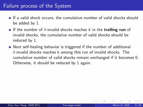
If a valid shock occurs, the cumulative number of valid shocks shouldbe added by 1.
If the number of δ-invalid shocks reaches k in the trailing run ofinvalid shocks, the cumulative number of valid shocks should bereduced by 1.
Next self-healing behavior is triggered if the number of additionalδ-invalid shocks reaches k among this run of invalid shocks. Thecumulative number of valid shocks remain unchanged if it becomes 0.Otherwise, it should be reduced by 1 again.
n : cumulative number of valid shocks that cause the system failured : cumulative number of valid shocks that make the system cometo the change point
Let us consider n = 5, d = 3, k = 2, δ = 1. Consider1′, 0′, 0I , (X1, . . . ,X11) indicate valid shocks, invalid shocks, the initialstate of the sequence of shocks and the time lags, respectively
Zhao, Guo, Wang (SME-BIT) Two-stage model March 31, 2020 8 / 25

Failure process of the System
If a valid shock occurs, the cumulative number of valid shocks shouldbe added by 1.
If the number of δ-invalid shocks reaches k in the trailing run ofinvalid shocks, the cumulative number of valid shocks should bereduced by 1.
Next self-healing behavior is triggered if the number of additionalδ-invalid shocks reaches k among this run of invalid shocks. Thecumulative number of valid shocks remain unchanged if it becomes 0.Otherwise, it should be reduced by 1 again.
n : cumulative number of valid shocks that cause the system failured : cumulative number of valid shocks that make the system cometo the change point
Let us consider n = 5, d = 3, k = 2, δ = 1. Consider1′, 0′, 0I , (X1, . . . ,X11) indicate valid shocks, invalid shocks, the initialstate of the sequence of shocks and the time lags, respectively
Zhao, Guo, Wang (SME-BIT) Two-stage model March 31, 2020 8 / 25
Illustration
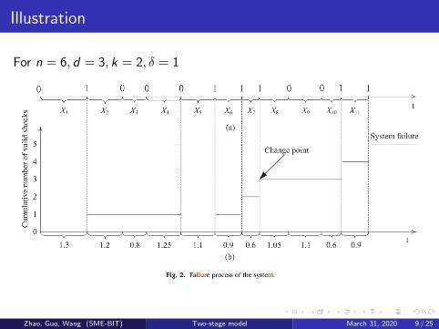
For n = 6, d = 3, k = 2, δ = 1
Zhao, Guo, Wang (SME-BIT) Two-stage model March 31, 2020 9 / 25

The Picturization of the two-stage model
Therefore essentially, the two-stage process looks like this:
Zhao, Guo, Wang (SME-BIT) Two-stage model March 31, 2020 10 / 25

Reliability Analysis of the shock model
Sm denotes the cumulative number of valid shocks.
Tm represents the number of δ-invalid shocks in the trailing run ofinvalid shocks.
Rm denotes the number of δ-invalid shocks which can trigger a nextself-healing behavior if the system is in stage 1 whereRm = Tm − [Tm
k ]k, otherwise, Rm = Θ where Θ means the system isin stage 2.
Markov chain Ym,m ≥ 0 associated with Sm and Rm is defined as
Ym = (Sm,Rm),m ≥ 0
Zhao, Guo, Wang (SME-BIT) Two-stage model March 31, 2020 11 / 25

The state-space
Ωm = (s, r) : 0 ≤ s ≤ d−1, 0 ≤ r ≤ k−1U(s,Θ) : d ≤ s ≤ n−1UEa
Initial State : Y0 = (0, 0)Ea: absorbing state, cumulative number of valid shocks reaches n and thesystem fails.
Zhao, Guo, Wang (SME-BIT) Two-stage model March 31, 2020 12 / 25

Forming the transition matrix
The probability q of invalid shock can be further broken down:
q1 = probability that m-th shock is δ-invalid.
q2 = probability that m-th shock is an invalid shock but not δ-invalid.(q1 + q2 = q)
Example: n = 4, d = 2, k = 2
Ωm = (0, 0), (0, 1), (1, 0), (1, 1), (2,Θ), (3,Θ)⋃Ea
Zhao, Guo, Wang (SME-BIT) Two-stage model March 31, 2020 13 / 25

The state transition diagram
Zhao, Guo, Wang (SME-BIT) Two-stage model March 31, 2020 14 / 25
One Step transition probability Matrix
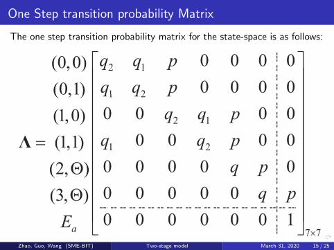
The one step transition probability matrix for the state-space is as follows:
Zhao, Guo, Wang (SME-BIT) Two-stage model March 31, 2020 15 / 25

Therefore the matrix Λ
can be written in general in the following format:
Where γ = [dk + (n − d + 1)] is the cardinality of the state-space Ω.
Zhao, Guo, Wang (SME-BIT) Two-stage model March 31, 2020 16 / 25

Λ can be transitioned as follows: Λ =
[P(γ−1)X (γ−1) Q(γ−1)X1
01X (γ−1) E1X1
]One step transition probabilities:
P(γ−1)X (γ−1) among transient states
Q(γ−1)X1 transient states to absorbing states
01X (γ−1) absorbing state to transient state
E1X1 identity matrix
Combining transient states in stage 2 and absorbing states into newabsorbing state Ef (system moves fromstage 1). Φ =[U(γ1)X (γ1) V(γ1)X1
01X (γ1) E1X1
]where γ1 = dXk
Zhao, Guo, Wang (SME-BIT) Two-stage model March 31, 2020 17 / 25

The general format of matrices P, Q,U and V
Zhao, Guo, Wang (SME-BIT) Two-stage model March 31, 2020 18 / 25

The distribution of N1
N1 is the total number of shocks until change point appears.Let α = (1, 0, . . . , 0)1Xγ1 , Ic = U0 and eγ1 = (1, . . . , 1)1Xγ1
The pmf of the shock length N1 is
P(N1 = k) = αUk−1V
The cdf of the shock length N1 is
P(N1 ≤ k) =k∑
i=1
αUi−1V
The expected shocklength is
E (N1) = α(Ic −U)−1e′γ1
Zhao, Guo, Wang (SME-BIT) Two-stage model March 31, 2020 19 / 25

The distribution of N2
N2 is the total number of shocks until the system fails.Let π0 = (1, 0, . . . , 0)1X (γ−1), I = P0 and e(γ−1) = (1, . . . , 1)1X (γ−1)The pmf of the shock length N2 is
P(N2 = k) = π0Pk−1Q
The cdf of the shock length N2 is
P(N2 ≤ k) =k∑
i=1
π0Pi−1Q
The expected shocklength is
E (N2) = π0(I− P)−1e′γ−1
Zhao, Guo, Wang (SME-BIT) Two-stage model March 31, 2020 20 / 25
Illustrative Example
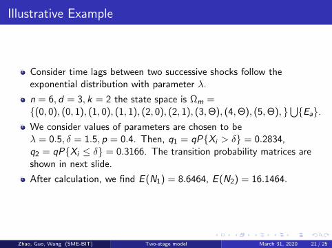
Consider time lags between two successive shocks follow theexponential distribution with parameter λ.
n = 6, d = 3, k = 2 the state space is Ωm =(0, 0), (0, 1), (1, 0), (1, 1), (2, 0), (2, 1), (3,Θ), (4,Θ), (5,Θ),
⋃Ea.
We consider values of parameters are chosen to beλ = 0.5, δ = 1.5, p = 0.4. Then, q1 = qPXi > δ = 0.2834,q2 = qPXi ≤ δ = 0.3166. The transition probability matrices areshown in next slide.
After calculation, we find E (N1) = 8.6464, E (N2) = 16.1464.
Zhao, Guo, Wang (SME-BIT) Two-stage model March 31, 2020 21 / 25
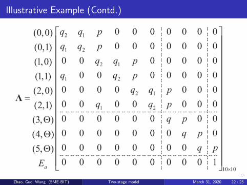
Illustrative Example (Contd.)
Zhao, Guo, Wang (SME-BIT) Two-stage model March 31, 2020 22 / 25

Illustrative Example (Contd.)
Zhao, Guo, Wang (SME-BIT) Two-stage model March 31, 2020 23 / 25

Table for some other choices of parameters
Zhao, Guo, Wang (SME-BIT) Two-stage model March 31, 2020 24 / 25

Thank you!
Zhao, Guo, Wang (SME-BIT) Two-stage model March 31, 2020 25 / 25