Reliability of individual valuations of public and private ... · Reliability of individual valuations of public and private goods: Choice consistency, response time, and preference

Journal of Public Economics 92 (2008) 1595–1606www.elsevier.com/locate/econbase

Reliability of individual valuations of public and private goods:Choice consistency, response time, and preference refinement

Thomas C. Brown a,⁎, David Kingsley b, George L. Peterson a, Nicholas E. Flores b,Andrea Clarke c, Andrej Birjulin d

a Rocky Mountain Research Station, U.S. Forest Service, 2150-A Centre Avenue, Fort Collins, Colorado 80526 USAb Department of Economics, University of Colorado, Boulder USA

c Natural Resources Conservation Service, Washington, DC 20250 USAd OMNI Institute, Denver, CO 80203 USA

Received 7 February 2007; received in revised form 11 October 2007; accepted 14 January 2008Available online 19 January 2008

Abstract

We examined the reliability of a large set of paired comparison value judgments involving public goods, private goods, andsums of money. As respondents progressed through a random sequence of paired choices they were each given, their response timedecreased and they became more consistent, apparently fine-tuning their responses, suggesting that respondents tend to begin ahypothetical value exercise with relatively imprecise preferences and that experience in expressing preference helps reduce thatimprecision. Reliability was greater for private than for public good choices, and greater for choices between a good and amonetary amount than for choices between two goods. However, the reliability for public good choices was only slightly lowerthan for the private goods.Published by Elsevier B.V.

JEL classification: D1; H41; Q20Keywords: Valuation; Reliability; Public goods; Response time; Preference learning

1. Introduction

How precisely do people know their preferences? It is common in applications of utility theory to assume thatpeople know their preferences perfectly. In modeling people's choices we therefore assume that error in estimation isattributable to missing variables or errors in measurement. But is this a reasonable assumption, especially when thepreferences are about unfamiliar goods?

According to McFadden (2001), Thurstone (1927) was the first to propose a choice model that allowed for, indeedexpected, errors in human judgment and preference. Thurstone had the advantage of years of prior research by fellowpsychologists into people's paired judgments of physical stimuli, such as the weights of objects or the loudness of

⁎ Corresponding author. Tel.: +1 970 295 5968; fax: +1 970 295 5959.E-mail address: [email protected] (T.C. Brown).

0047-2727/$ - see front matter. Published by Elsevier B.V.doi:10.1016/j.jpubeco.2008.01.004

1596 T.C. Brown et al. / Journal of Public Economics 92 (2008) 1595–1606

sounds, which demonstrated that people's accuracy in judging the relative magnitudes of such stimuli decreased as thedifference between the stimuli lessened (Brown and Peterson, 2003). He extended this finding to the domain ofpreferences (e.g., Thurstone and Chave, 1929) and developed a theory and method for estimating the relativemagnitudes of the stimuli, using the amount of inconsistency in preference as an indication of the closeness of thestimuli.

The possibility of error—or, more precisely, imprecision or uncertainty—in individual preference as proposed byThurstone did not go unnoticed over the years. As McFadden explains, Marschak (1959) brought the idea to theattention of economists. Although economists' adaptation of the random utility notion focused on exogenous sourcesof error, endogenous error has been mentioned occasionally over the years by economists (e.g., Hausman and Wise,1978) and is gradually becoming more accepted (e.g., Ben-Akiva and Lerman, 1985; Bockstael and Strand, 1987; Liand Mattsson, 1995; Rieskamp et al., 2006).

Survey methods such as contingent valuation or conjoint (multi-attribute) analysis have emerged as primarymethods for estimating the economic value of public goods. With these methods we rely on people's responses toquestions about their willingness to pay (WTP) for a certain good or on their choices among goods that are eachavailable at a price. These methods were initially used to value quasi-private nonmarket goods, such as an individualrecreation opportunity on public land, or, in the case of conjoint analysis, consumer goods, but the methods have beenextended to value public goods such as air quality protection and wilderness preservation. Many contingent valuationstudies (see Carson et al., 1994) and several conjoint studies have valued public goods. However, the extension topublic goods incurs potential problems related to, among other things, respondents' lack of familiarity with purchasingsuch goods.

The question about how well people know their preferences has been addressed, within contingent valuation, in partvia reliability studies. Some of these studies used the test–retest approach, where a sample is asked the same questionon two different occasions. Time periods between tests have varied from a few weeks to several years, and both publicand private goods have been studied. In all cases significant correlations were found between the two occasions; mostcorrelations fell in the 0.5 to 0.8 range (see Jorgensen et al., 2004; McConnell et al., 1998 for summaries of thesestudies). Other studies used different samples at different times and compared estimates of meanWTP (Jorgensen et al.,2004; McConnell et al., 1998 list some of these), generally finding no significant difference between the estimates.

These studies provide a general sense of confidence in the contingent valuation method, but they do not deal directlywith the question posed above, about the precision with which a given subject is able to respond to a WTP question.They also do not help us understand whether subjects learn about their preferences in the course of forming an answer.The studies are unable to address these questions because they ask each respondent only one or a few monetaryvaluation questions. Our methods, because we ask each respondent a large number of valuation questions, help answerthese questions. Most importantly, our methods allow us to observe and test for changes in the consistency ofpreferences as respondents proceed through the multiple valuation questions they are given.

Despite the fact that the reliability of stated WTP has been found to be adequate in the studies referred to above, ithas long been thought that reliability would be substantially less for public than for private goods (Cummings et al.,1986), principally because public goods lack market prices and people have less experience valuing them. Only onestudy, by Kealy et al. (1990), tested this conjecture. The authors obtained WTP estimates for a private good and a publicgood from separate samples, and then replicated those estimates with the same two groups two weeks later. They foundthat the test–retest reliability of the estimate for the public good was only slightly less than, and not significantlydifferent from, that of the private good estimate, thereby rejecting the Cummings et al. conjecture. We took a secondlook at this issue by including both public and private goods in our surveys.

Our approach uses the paired comparison (PC) method, which dates back to Fechner (1860) and has been studiedextensively (e.g., Bock and Jones, 1968; David, 1988; Thurstone, 1927; Torgerson, 1958). The method yields anindividual respondent's preference order among items of a choice set by presenting the items in pairs and askingrespondents to choose the item in each pair that best meets a given criterion, such as being the more preferred.Importantly for our purposes here, the method yields individual estimates of reliability.

The PC method asks each respondent to make numerous binary choices. When all possible pairs of the items arepresented and the number of items is large enough that respondents have difficulty recalling past choices, the methodoffers abundant opportunities for inconsistency in preference, which allow for our first approach to reliability. Inaddition, we repeated some of the pairs at the end of the session, offering a short-term test–retest measure of reliability.We report on these two approaches for assessing reliability for public and private good choices, and also examine how

1597T.C. Brown et al. / Journal of Public Economics 92 (2008) 1595–1606

response time and consistency of preference changes over the course of a session and how response time varies by typeof choice (public or private good) and by consistency of the choice.

2. Conceptual model

As proposed by Thurstone (1927) in his exposition on paired comparisons, preferences are probably best describedby a stochastic function. This function is now commonly known as a random utility function in recognition of the beliefthat the true utilities of the items are the expected values of preference distributions. The random utility function (U)consists of deterministic (V) and random (ε) components.1 For example, the utility of items 1 and 2 to respondent i onchoice occasion j can be represented by the following two relations:

Uij1 ¼ Vi1 þ eij1Uij2 ¼ Vi2 þ eij2

: ð1Þ

The randomness signified by ε in the current application is inherent in the individual choice process, which issubject to fluctuations and disturbances that are beyond our ability to model deterministically. Among a respondent'schoices in a PC exercise, this variation has at least three potential sources. First, choices are subject to measurementerror, which occurs, for example, when a respondent mistakenly pushes the wrong key or checks the wrong box torecord a choice. Second, preferences may be subject to momentary fluctuations resulting from preference imprecision(Thurstone, 1927). Third, preference for multi-attribute items may vary with the mix of attributes of the pair of itemsbeing compared. This may occur, for example, when respondents weight attributes differently when making differentcomparisons (Tversky, 1969), make different assumptions about incompletely described items when making differentcomparisons, or have multiple objective functions (Hicks, 1956) and focus on different objectives when makingdifferent comparisons.

The probability of an individual selecting item 1 in a comparison of items 1 and 2 is given by:

P Uij1NUij2

� � ¼ P Vi1 þ eij1NVij2 þ eij1� �

: ð2Þ

This probability P is greater the larger is V1−V2 and the narrower are distributions of ε1 and ε2. An inconsistentresponse occurs when Uij2NUij1 although Vi1NVi2, and can happen when the distributions of εij1 and εij2 about theirrespective Vs overlap.

We suspect, in line with the Cummings et al. (1986) conjecture, that ε will tend to be wider when the items lackmarket prices and when respondents have little experience valuing them. Because these conditions are more often thecase with public than with private goods, we hypothesize that reliability will be lower for public good choices than forprivate good choices. Similarly, we hypothesize that respondents will take more time to make public than private goodchoices and that inconsistent choices will take more time than consistent choices.

In each PC session, respondents made over 100 choices among all possible pairs of the items. As respondents workthrough the sequence of choices they may fine-tune their preferences. Perhaps the most likely change with sequence isa narrowing of the disturbance term as respondents become more settled in their preferences. We hypothesize such anarrowing, and thus a drop in ε with sequence.

3. Methods

For this paper we combined data from three studies. Each study focused on specific valuation issues apart from thereliability concerns of this paper, but all three studies used the same basic procedure for eliciting PC responses,enabling us to aggregate the data to evaluate two measures of respondent reliability, one based on isolation ofinconsistent choices among the original choices and the other relying on a retest of the original choices. In this section,the PC procedure and the data it provides are described and our analysis procedures are summarized.

1 Thurstone thought of ε a normally distributed about mean V, leading to a random utility function that is now characterized using the binaryprobit model. Other distributional forms for ε are feasible and commonly assumed in modern discrete choice analysis (Ben-Akiva and Lerman,1985).

Table 1Data sources

Study Number ofrespondents

Number of goods Number of moneyamounts

Number of choices perrespondent

Public Private

Birjulin (1997) 189 6 4 11 155Clarke et al. (1999) 463 5 4 8 108Peterson and Brown (1998) 327 6 4 11 155Total 979


3.1. The data

The three studies that provided the data for this paper (Table 1) each obtained judgments for a mixture of publicgoods, private goods, and amounts of money.2 Some goods were used in more than one study, but most were unique toa specific study. Across the three studies, a total of 979 respondents, all university students, provided PC judgments. Allpublic goods were locally relevant, involving the university campus or its surrounding community. All private goodswere common consumer items with specified prices. In total, these three studies yielded 129,984 respondent choices,each between a pair of items.

As an example of the methods of these three studies, we summarize the methods used by Peterson and Brown(1998). The choice set consisted of six public goods, four private goods, and eleven sums of money (21 items in total).Each respondent made 155 choices consisting of 45 choices between goods and 110 choices between goods and sumsof money. They did not choose between sums of money (it was assumed that larger amounts of money were preferred tosmaller ones), but did choose between all other possible pairs of the items. The 327 respondents yielded a total of50,685 binary choices.

The four private goods of the Peterson and Brown (1998) study were: a meal at any local restaurant, not to exceed acost of $15; a $200 certificate useable at any local clothing store; a $500 certificate for air travel on any airline; and twotickets for one of four listed events (e.g., a professional football game) with an estimated value of $75. The six publicgoods were of mixed type. Two were pure public environmental goods, in that they were nonrival and nonexcludable inconsumption. One was the purchase by the university of 2000 acres of land in the mountains west of town as a wildliferefuge for animals native to the area; the other focused on clean air and water. The remaining four public goods wereexcludable by nature but stated as nonexcludable by policy, and were nonrival until demand exceeds capacity. One wasa no-fee library service that provides video tapes of all course lectures; the others involved campus parking capacity, acampus music festival, and student dining facilities. The eleven sums of money were $1, $25, $50, $75, and $100 to$700 in intervals of one hundred. These amounts were derived from pilot studies in order to have good variation anddistribution across the values of the goods.

Respondents were asked to choose one or the other item under the assumption that either would be provided at nocost to the respondent. The respondent simply chose the preferred item in each pair. If respondents were indifferentbetween the two items in a pair, they were still asked to make a choice; indifference across respondents was laterrevealed as an equal number of choices of each item.3

The surveys were administered on personal computers that presented the pairs of items on the monitors in randomorder for each respondent to control for order effects. The items appeared side-by-side on the monitor, with theirposition (right versus left) also randomized. The respondent entered a choice by pressing the right or left arrow key and,as long as a subsequent choice had not yet been entered, could correct a mistake by pressing the backspace key and thenselecting the other item. Review of prior choices was not possible. At the end of the original paired comparisons, thecomputer presented some of the pairs a second time, without a break in the presentation and without a priorannouncement that some pairs would be repeated. The pairs presented for retrial were of two kinds, those pairs for

2 Complete lists of the goods are found in chapter 2 of the Discussion Paper “An enquiry into the method of paired comparison: Reliability,scaling, and Thurstone's law of comparative judgment” available at http://www.fs.fed.us/rm/value/discpapers.html.3 Providing subjects with an indifference option may have its advantages. If it worked well, it would allow us to separate real indifference from

other sources of inconsistency. However, providing an indifference option runs the risk of allowing subjects to avoid all close calls. If, as Torgerson(1958) argues, the probability of true indifference at any given time is “vanishingly small,” forcing a choice maximizes the amount learned whilestill allowing indifference to be revealed in data from multiple subjects or from a given subject responding multiple times.


which the individual's choice was not consistent with the dominant preference order as defined by the preference scores(see the definition of preference score below), and ten randomly selected consistent pairs. The individual pairs in thesetwo sets of repeated choices were randomly intermixed. The computer also recorded the time taken to enter eachchoice. Respondents were not told that response time was recorded.

3.2. Data analysis

Given a set of t items, the PC method presents them independently in pairs as (t / 2)(t−1) discrete binary choices.These choices yield a preference score for each item, which is the number of times the respondent prefers that item toother items in the set. A respondent's vector of preference scores describes the individual's preference order among theitems in the choice set, with larger integers indicating more preferred items. In the case of a 21-item choice set, anindividual preference score vector with no circular triads contains all 21 integers from 0 through 20. Circular triads (i.e.,choices that imply ANBNCNA) cause some integers to appear more than once in the preference score vector, whileothers disappear.

For a given respondent, a pair's preference score difference (PSD) is simply the absolute value of the differencebetween the preference scores of the two items of the pair. This integer, which can range from 0 to 20 for a 21-itemchoice set, indicates on an ordinal scale the difference in value assigned to the two items.

The number of circular triads in each individual's responses can be calculated directly from the preference scores.The number of items in the set determines the maximum possible number of circular triads. The individualrespondent's coefficient of consistency is calculated by subtracting the observed number of circular triads from themaximum number possible and dividing by the maximum.4 The coefficient varies from one, indicating that there are nocircular triads in a person's choices, to zero, indicating the maximum possible number of circular triads.

When a circular triad occurs, it is not unambiguous which choice is the cause of the circularity. This is easily seen byconsidering a choice set of three items, whose three paired comparisons produce the following circular triad:ANBNCNA. Reversing any one of the three binary choices removes the circularity of preference; selection of the one tolabel “inconsistent” is arbitrary. However, with more items in the choice set, selection of inconsistent choices (i.e.,choices where Uij2NUij1 although Vi1NVi2), though still imperfect, can be quite accurate. For each respondent, weselected as inconsistent any choice that was contrary to the order of the items in the respondent's preference scorevector, with the condition that the order of items with identical preference scores was necessarily arbitrary. Simulationsshow that the accuracy of this procedure in correctly identifying inconsistent choices increases rapidly as the PSDincreases. In simulations with a set of 21 items and assuming normal dispersion distributions, the accuracy of theprocedure rises quickly from 50% at a PSD of 0 to nearly 100% at a PSD of 5. Simulations also show that the procedureis unbiased and thus can be used to compare consistency across sets of choices, such as sets representing differentclasses of goods or different points along the sequence of choices (e.g., first pair versus second pair).5

The proportion of choices that were selected as inconsistent, across all respondents, provides another measure ofreliability. We computed this measure for all choices together, and then for three partitions of the data. First, themeasure was computed for each choice in the order the choices were made (i.e., it was computed for all the first choices,all the second choices, etc.). Plotting the proportion inconsistent for each choice, with the choices in sequence, showshow inconsistency changes as respondents gain more experience with the choice task and the items being compared.6

Because the pairs were presented in a unique random order to each respondent, this measure is independent of pair

4 The maximum possible number of circular triads, m, is (t / 24)(t2−1) when t is an odd number and (t / 24)(t2−4) when t is even, where t is thenumber of items in the set. Letting ai equal the preference score of the ith item and b equal the average preference score (i.e., (t−1) /2), the numberof circular triads is (David, 1988):

c ¼ t24

t2 � 1� �� 1

2

Xai � bð Þ2:

The coefficient of consistency (Kendall and Smith, 1940) is then defined as: 1−c/m.5 A thorough explanation of the procedure for specifying inconsistent choices is found in chapter 4 of the Discussion Paper “An enquiry into the

method of paired comparison: Reliability, scaling, and Thurstone's law of comparative judgment” available at http://www.fs.fed.us/rm/value/discpapers.html.6 Attribute-based choice studies that have evaluated change in consistency over the sequence of choices include Swait and Adamowicz (2001),

who employed 16 choices, and Holmes and Boyle (2005) who examined 4 choices.

Fig. 1. Distribution of respondent reliability.


order. Second, the measure was computed for the five different types of choices: private good versus money, publicgood versus money, private good versus private good, public good versus public good, and private good versus publicgood. Third, the measure was computed for each level of PSD to show how inconsistency changes as the choicesbecome easier to make. We performed numerous statistical tests on these measures of inconsistency, either to compareresults for public goods with those for private goods, or to evaluate trends over time. Proportions were compared usinga test based on the normal approximation to the binomial distribution. Trends were evaluated using linear regression.For all tests, we used a 0.05 probability level to test for significance.

Because our procedure is uncommon, we also used a more well-recognized method, a heteroscedastic probitimplementation of the random utility model, to evaluate the reliability of respondents' choices. This very differentmethod provides a check on the preference-score-based approach. The probit analysis uses the variance of thedisturbance term (ε, Eq. (1)) as the measure of inconsistency (DeShazo and Fermo, 2002; Swait and Adamowicz,1996). This approach confirmed the findings obtained based on our simple decision rule for isolating inconsistentchoices, both in examination of changes in inconsistency with sequence and in comparing inconsistency of public andprivate good choices. To conserve space here, the methods and results of the probit analysis are described elsewhere.7

As a final measure of reliability we use the repeats of originally consistent choices (For completeness, we alsopresent the data on the repeats of inconsistent pairs.). Choice switching (i.e., choosing one item initially and the otheritem upon retrial) when an originally consistent choice was made indicates a lack of reliability.

4. Results

Results from the original choices are presented in Subsections 4.1–4.5, followed by results from the repeatedchoices in Subsection 4.6. All results shown in figures or reported in tables are based on the full set of 979 respondents.

4.1. Coefficient of consistency

Coefficients of consistency were computed for each respondent. The mean coefficients of the three studies rangefrom 0.908 to 0.915, and the median coefficients range from 0.927 to 0.939. In each set, the median exceeds the mean,as the means are sensitive to the relatively low coefficients of a minority of respondents in each set (Fig. 1). The overallmedian coefficient is 0.93; 95% of the respondents had a coefficient of at least 0.77.

4.2. Change in consistency with sequence

Across the three studies, 7.2% of the choices were inconsistent with respondents' dominant preference orders asdetermined by the preference score vector. To examine how this inconsistency varies over time, the proportion of

7 See the Discussion Paper “Paired comparisons of public and private goods, with heteroscedastic probit analysis of choice consistency” found athttp://www.fs.fed.us/rm/value/discpapers.html.

Fig. 2. Proportion of respondents making an inconsistent choice, first 100 choices.


choices that were inconsistent was computed for each choice in sequence (i.e., all first choices, all second choices, etc.).As Fig. 2 shows, inconsistency drops from 15% for the first choice to about 7% by the 30th choice, and then dropsonly slightly more after that (all three studies show the same pattern). The drop in inconsistency that occurs overthe first 30 pairs is highly significant (df=29, F=116.06, pb0.01), but the slight drop from the 31st to the 100th choiceis not significant (df=29, F=2.95, p=0.09).8 A minimum level of inconsistency, which is roughly 6.5% for thesedata (Fig. 2), is always expected, largely because some of the choices are between items of roughly equal desirability(i.e., they are close calls). Because each respondent encountered the choices in a unique random order, Fig. 2 is notdependent on the nature of the particular items that were first encountered. The drop in inconsistency over timesuggests that respondents were fine-tuning or firming up the preferences with which they began the PC exercise.

The changing consistency with sequence depicted in Fig. 2 suggests that respondents were narrowing the mag-nitudes of the random components of their preference distributions (ε) over the course of the session, but it does noteliminate the possibility that respondents' preferences (V) were also changing with sequence. The sample sizes of thethree studies are insufficient for computing average preference scores for each item for each choice in the sequence ofchoices, but we can compare average preference scores from sets of choices, such as sets of early versus late choices.9

A comparison of the average preference scores estimated from the first 30 choices with those estimated from choices71–100 produced correlations of early versus late average preference scores ranging from 0.96 to 0.99 across the threestudies, indicating very little shift in preferences with sequence, thus supporting the claim that only the disturbanceterms were changing over the course of the sessions.

4.3. Response time

Mean response (decision) times for the second through the sixth choices were 10.0, 8.0, 6.7, 6.3, and 6.0 s. Responsetime continued to drop at a decreasing rate until about halfway through the choices, when it stabilized at about 2.4 s.Response times were longer for inconsistent than for consistent choices. Indeed, for every one of the first 100 choices,inconsistent choices took more time on average than did consistent choices (Fig. 3), a result that is extremely unlikelyto occur by chance alone. On average, consistent choices took 3.4 s and inconsistent choices took 4.7 s.

4.4. Inconsistency and preference score difference

Fig. 4 shows that inconsistency decreases rapidly with PSD.10 Fifty percent of the choices are inconsistent at azero PSD, as expected. Inconsistency drops to 1% by a PSD of 8. Seventy-two percent of all inconsistent choices

8 Figures of choices by sequence show only the first 100 choices, which is sufficient to depict the trend and avoids including later choices, someof which are based on only a subset of the respondents (as shown in Table 1, the total number of choices varied by study). In any case, we found notrends in proportion inconsistent past the 100th choice (e.g., no evidence of fatigue, which could cause an increase in inconsistency).9 For a given study and set of sequential choices, the average preference score of each item was computed as the number of times, across all

respondents, the item was chosen over the number of times the item appeared among the choices. Such computations are possible because of therandom ordering of pairs for each respondent.10 Because the Clarke et al. (1999) data set includes only 18 items, the contribution to Fig. 4 from that data set is limited to PSDs of from 0 to 17.

Fig. 3. Mean response time, 2nd through 100th choice.

Fig. 4. Inconsistency versus preference score difference.


occurred at a PSD≤2. The fact that inconsistency drops to near zero for choices of high PSD indicates that mistakes,which would not be restricted to choices of low PSD, are not a major cause of inconsistent choices. The fact that 72% ofthe inconsistent choices occur at a PSD≤2 suggests that most inconsistent choices result from indifference or nearindifference.

Further, mean response time dropped monotonically with mean PSD, from 5 s at PSD=0 to about 2 s at PSD=20,indicating that people labor more over close calls than obvious ones.11 That close calls are the most difficult ones is, ofcourse, not news to anyone who has fretted over a choice between two equally good options.

Although most inconsistent choices involve close calls, a substantial amount (28%) of the inconsistent choicesoccurred at PSDN2, indicating a rather high degree of imprecision. The data show that many of these inconsistentchoices were produced by a minority of respondents. For example, one-half of the inconsistent choices of PSDN2 wereproduced by the 20% of the respondents with the lowest coefficients of consistency, as might be anticipated from Fig. 1.

The finding that over one quarter of the inconsistent choices involve pairs with a rather large PSD, and that mistakesaccount for very few of the inconsistent choices, raises the question: when do these high PSD inconsistent choicesoccur? Are they sprinkled evenly over the sequence of pairs, or are they concentrated among the first few pairs? Asshown in Fig. 5, inconsistent choices of higher PSD are more common early in the sequence. The mean PSDs of thefirst few pairs are near 3, mean PSD drops over the first 30 pairs or so, and after the 30th pair the mean PSDs are nearlyall below 2, averaging 1.73. Regression shows that the slope of the straight line fitted for first 30 points is significantlynegative (df=29, F=52.54, pb0.01), and that the subsequent points show no slope (df=69, F=1.65, p=0.20). If weaccept the conceptual model of the choice process represented by Eq. (1), this finding suggests again that respondents

11 Response time increases not only with the closeness of the items being compared. A study by Wilcox (1993) of choices between lotteries foundthat decision time increased with the complexity of the lotteries; and a recent study by Rubinstein (2007) posits, based on subjects' choices inseveral complex games, that choices made instinctively take less time than choices made using cognitive reasoning.

Fig. 5. Mean preference score difference, first 100 choices.


begin the exercise with relatively imprecise values (i.e., relatively large disturbance terms ε) and that the disturbancegradually narrows as respondents gain experience with the items in the course of comparing them.

Also shown in Fig. 5 are the mean PSDs of the consistent choices. These mean PSDs are considerably larger thanthose of the inconsistent choices, averaging 6.78 across the first 100 pairs in comparison to 1.90 for the inconsistentchoices. Mean PSD is larger for consistent choices because choices for pairs with a large PSD tend to be consistent.There is no trend in mean PSD over sequence for the consistent choices.

4.5. Separating public and private goods

Separating the public good choices from the private good choices shows that both classes of goods follow thepattern shown in Fig. 2, but that the degree of inconsistency is slightly greater for public good than for private goodchoices (Fig. 6). The public good choices are those involving only public goods or public goods and dollars, and theprivate good choices are those involving only private goods or private goods and dollars (thus, this breakdown ignoresthe choices comparing a public good with a private good). For 62 of the first 100 choices, public good choices were lessconsistent than private good choices (0.62 is significantly greater than 0.5). The greatest differences occur among thefirst 14 choices, but the tendency for inconsistency to be greater for public than for private goods persists throughoutthe sequence of choices. Ignoring sequence, 7.0% of the 64,946 public good choices and 6.5% of the 43,394 privategood choices were inconsistent (the two percentages are significantly different).

Response times were also longer for public good choices, taking an average of 3.5 s compared with 3.3 s for privategood choices. Although the difference is small, it was persistent; for example, mean public good response times werelonger than mean private good response times for 86 of the first 100 choices.

Fig. 6. Proportion of respondents making an inconsistent choice, for public and private good choices, first 100 choices.

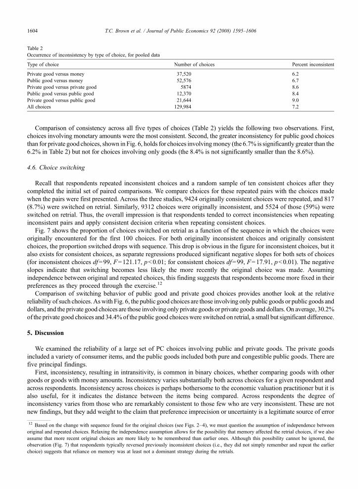
Table 2Occurrence of inconsistency by type of choice, for pooled data

Type of choice Number of choices Percent inconsistent

Private good versus money 37,520 6.2Public good versus money 52,576 6.7Private good versus private good 5874 8.6Public good versus public good 12,370 8.4Private good versus public good 21,644 9.0All choices 129,984 7.2


Comparison of consistency across all five types of choices (Table 2) yields the following two observations. First,choices involving monetary amounts were the most consistent. Second, the greater inconsistency for public good choicesthan for private good choices, shown in Fig. 6, holds for choices involvingmoney (the 6.7% is significantly greater than the6.2% in Table 2) but not for choices involving only goods (the 8.4% is not significantly smaller than the 8.6%).

4.6. Choice switching

Recall that respondents repeated inconsistent choices and a random sample of ten consistent choices after theycompleted the initial set of paired comparisons. We compare choices for these repeated pairs with the choices madewhen the pairs were first presented. Across the three studies, 9424 originally consistent choices were repeated, and 817(8.7%) were switched on retrial. Similarly, 9312 choices were originally inconsistent, and 5524 of those (59%) wereswitched on retrial. Thus, the overall impression is that respondents tended to correct inconsistencies when repeatinginconsistent pairs and apply consistent decision criteria when repeating consistent choices.

Fig. 7 shows the proportion of choices switched on retrial as a function of the sequence in which the choices wereoriginally encountered for the first 100 choices. For both originally inconsistent choices and originally consistentchoices, the proportion switched drops with sequence. This drop is obvious in the figure for inconsistent choices, but italso exists for consistent choices, as separate regressions produced significant negative slopes for both sets of choices(for inconsistent choices df=99, F=121.17, pb0.01; for consistent choices df=99, F=17.91, pb0.01). The negativeslopes indicate that switching becomes less likely the more recently the original choice was made. Assumingindependence between original and repeated choices, this finding suggests that respondents become more fixed in theirpreferences as they proceed through the exercise.12

Comparison of switching behavior of public good and private good choices provides another look at the relativereliability of such choices.Aswith Fig. 6, the public good choices are those involving only public goods or public goods anddollars, and the private good choices are those involving only private goods or private goods and dollars. On average, 30.2%of the private good choices and 34.4%of the public good choiceswere switched on retrial, a small but significant difference.

5. Discussion

We examined the reliability of a large set of PC choices involving public and private goods. The private goodsincluded a variety of consumer items, and the public goods included both pure and congestible public goods. There arefive principal findings.

First, inconsistency, resulting in intransitivity, is common in binary choices, whether comparing goods with othergoods or goods with money amounts. Inconsistency varies substantially both across choices for a given respondent andacross respondents. Inconsistency across choices is perhaps bothersome to the economic valuation practitioner but it isalso useful, for it indicates the distance between the items being compared. Across respondents the degree ofinconsistency varies from those who are remarkably consistent to those few who are very inconsistent. These are notnew findings, but they add weight to the claim that preference imprecision or uncertainty is a legitimate source of error

12 Based on the change with sequence found for the original choices (see Figs. 2–4), we must question the assumption of independence betweenoriginal and repeated choices. Relaxing the independence assumption allows for the possibility that memory affected the retrial choices, if we alsoassume that more recent original choices are more likely to be remembered than earlier ones. Although this possibility cannot be ignored, theobservation (Fig. 7) that respondents typically reversed previously inconsistent choices (i.e., they did not simply remember and repeat the earlierchoice) suggests that reliance on memory was at least not a dominant strategy during the retrials.

Fig. 7. Proportion of choices switched upon retrial, first 100 choices.


within the random utility maximization model, and that the standard assumption in utility theory that the consumerknows her preferences precisely is unrealistic.

Second, response time varies systematically across types of choices, being longer for early as opposed to laterchoices, inconsistent as opposed to consistent choices, and close calls as opposed to more obvious choices. If we acceptresponse time as an indication of choice difficulty, we have some evidence that difficulty increases with closeness of theitems in the pair, and that choices become less difficult with experience choosing among the items.

Third, reliability improved dramatically over the course of the first 30 or so choices. Further, we found no evidencethat values (Vs) were changing. Respondents were apparently firming up their preferences as they consideredadditional choices involving the same items. In terms of Eq. (1), the variances of the disturbance distributions (ε)diminished with sequence. This finding supports the hypothesis that most respondents begin a hypothetical valueexercise with relatively imprecise preferences about the items presented and that experience in expressing preferenceabout the items helps to reduce that imprecision. This increasing precision is consistent with the notion of “valuelearning,” a component of preference learning, proposed by Braga and Starmer (2005), but only in the limited sense offirming up of preferences, not in the sense of changing preferences, and is perhaps more aptly called preferencerefinement.13 The evidence implies that a valuation study that relies on only one choice per respondent, as is commonin contingent valuation, for example, may be unduly limiting the reliability of its value estimate.

Increasing precision of preference (i.e., narrowing of ε) as respondents become more familiar with the items beingcompared is not the only explanation for the observed improvement in consistency with sequence. It is also possible thatrespondents gradually develop simplifying rules for making difficult choices and then use those rules for all choicesexcept those for which there are overwhelming reasons to ignore the rule. One example of such a rule would be thatpeople tend to cue on specific attributes. For example, a person might tend to choose a public good over a private goodwhenever the values of the two goods are similar. We suspect that some people do use simplifying rules, but we have noway of knowing how common such behavior is. Future research should strive to determine the relative importance of thedifferent possible explanations for the improving consistency with experience choosing among the items.

The fourth finding is that reliability was generally greater for private good than for public good choices, andgenerally greater for choices involving a monetary amount than for choices comparing two goods. This is in contrast tothe study by Kealy et al. (1990), who found a similar but insignificant difference for private versus public goods. Wehypothesize that our findings reflect the degree to which people have experience trading such items. Monetary amountswere the most commonly traded items of the choice sets, and private goods are more commonly traded than publicgoods. Further, the private goods had specified prices, which may help to anchor their values. Lack of experiencevaluing an item may tend to widen the distribution of its value, leading to more close calls, and thus to more circulartriads, inconsistent choices, and switches on retrial.

13 Our findings on preference refinement bring to mind the controversy regarding the learning about one's preferences that occurs over repeatedtrials of some choice task (Braga and Starmer, 2005, cite many of the relevant papers). Some authors adhere to the discovered preference hypothesisproposed by Plott (1996), which maintains that stable (i.e., context independent) underlying preferences are discovered through sufficient repetitionof a choice task that provides relevant feedback. Others counter, especially when dealing with unfamiliar goods, that labile (i.e., context dependent)preferences are constructed in the course of choosing (Gregory et al., 1993), and that repetition of the choice task in the same context will not alterthe effects on preference of contextual cues. Unfortunately, because the task we presented to respondents involved no consequences and feedback,and because we did not specifically test for the effect of contextual cues, we can offer no insight on the controversy.


Finally, the reliability for public good choices was only slightly lower than for the private good choices. Althoughwe found significant differences in consistency between the two classes of goods, those differences were small. Basedon this and earlier evidence, reliability of public good choices does not appear to be a major concern. The validity ofstated-preference estimates of economic value of public goods is a separate issue.

References

Ben-Akiva, M., Lerman, S.R., 1985. Discrete Choice Analysis: Theory and Application to Travel Demand. Massachusetts Institute of Technology,Cambridge, MA.

Birjulin, A.A., 1997. Valuation of public goods using the method of paired comparison: the effects of psychological distance between goods onconsistency of preferences. Unpublished dissertation, Colorado State University, Fort Collins, CO.

Bock, R.D., Jones, L.V., 1968. The Measurement and Prediction of Judgment and Choice. Holden-Day, Inc., San Francisco, CA.Bockstael, N.E., Strand Jr., I.E., 1987. The effect of common sources of regression error on benefit estimates. Land Economics 63 (1), 11–20.Braga, J., Starmer, C., 2005. Preference anomalies, preference elicitation and the discovered preference hypothesis. Environmental and Resource

Economics 32 (1), 55–89.Brown, T.C., Peterson, G.L., 2003. Multiple good valuation. In: Champ, P.A., Boyle, K., Brown, T.C. (Eds.), A primer on non-market valuation.

Kluwer Academic Publishers, Norwell, MA, pp. 221–258.Carson, R.T., Wright, J., Carson, N., Alberini, A., Flores, N., 1994. A bibliography of contingent valuation studies and papers. Natural Resource

Damage Assessment, Inc., La Jolla, CA.Clarke, A., Bell, P.A., Peterson, G.L., 1999. The influence of attitude priming and social responsibility on the valuation of environmental public

goods using paired comparisons. Environment and Behavior 31 (6), 838–857.Cummings, R.G., Brookshire, D.S., Schulze, W.D. (Eds.), 1986. Valuing Environmental Goods: An Assessment of the Contingent Valuation Method.

Rowman and Allanheld, Totowa, NJ.David, H.A., 1988. The Method of Paired Comparisons (Second ed. Vol. 41). Oxford University Press, New York, NY.DeShazo, J.R., Fermo, G., 2002. Designing choice sets for stated preference methods: the effects of complexity on choice consistency. Journal of

Environmental Economics and Management 44 (1), 123–143.Fechner, G.T., 1860. Elemente der psychophysik. Breitkopf and Hartel, Leipzip.Gregory, R., Lichtenstein, S., Slovic, P., 1993. Valuing environmental resources: a constructive approach. Journal of Risk and Uncertainty 7, 177–197.Hausman, J.A., Wise, D.A., 1978. A conditional probit model for qualitative choice: discrete decisions recognizing interdependence and het-

erogeneous preferences. Econometrica 46 (2), 403–426.Hicks, J.R., 1956. A Revision of Demand Theory. Oxford University Press, London.Holmes, T.P., Boyle, K.J., 2005. Dynamic learning and context-dependence in sequential, attribute-based, stated-preference valuation questions.

Land Economics 81 (1), 114–126.Jorgensen, B.S., Syme, G.J., Smith, L.M., Bishop, B.J., 2004. Random error in willingness to pay measurement: a multiple indicators, latent variable

approach to the reliability of contingent values. Journal of Economic Psychology 25 (1), 41–59.Kealy, M.J., Montogmery, M., Dovidio, J.F., 1990. Reliability and predictive validity of contingent values: does the nature of the good matter?

Journal of Environmental Economics and Management 19, 244–263.Kendall, M.G., Smith, B.B., 1940. On the method of paired comparisons. Biometrika 31, 324–345.Li, C.-Z., Mattsson, L., 1995. Discrete choice under preference uncertainty: An improved structural model for contingent valuation. Journal of

Environmental Economics and Management 28, 256–269.Marschak, J., 1959. Binary-choice constraints and random utility indicators. Paper presented at the Mathematical Methods in the Social Sciences.

Stanford University Press.McConnell, K.E., Strand, I.E., Valdes, S., 1998. Testing temporal reliability and carry-over effect: the role of correlated responses in test–retest

reliability studies. Environmental and Resource Economics 12 (3), 357–374.McFadden, D., 2001. Economic choices. American Economic Review 91 (3), 351–378.Peterson, G.L., Brown, T.C., 1998. Economic valuation by the method of paired comparison, with emphasis on evaluation of the transitivity axiom.

Land Economics 74 (2), 240–261.Plott, C.R. 1996. Rational individual behavior in markets and social choice processes: The discovered preference hypothesis. In K. Arrow, E.

Colombatto, M. Perleman, C. Schmidt (Eds.), Rational foundations of economic behavior, pp. 225–250. London: Macmillan and St. Martin's.Rieskamp, J., Busemeyer, J.R., Mellers, B.A., 2006. Extending the bounds of rationality: evidence and theories of preferential choice. Journal of

Economic Literature 44 (3), 631–661.Rubinstein, A., 2007. Instinctive and cognitive reasoning: a study of response times. Economic Journal 117, 1243–1259.Swait, J., Adamowicz, W., 1996. The effect of choice complexity on random utility models: an application to combined stated and revealed preference

models. Working Paper, Department of Marketing, University of Florida, Gainsville, FL.Swait, J., Adamowicz, W., 2001. The influence of task complexity on consumer choice: a latent class model of decision strategy switching. Journal of

Consumer Research 28 (1), 135–148.Thurstone, L.L., 1927. A law of comparative judgment. Psychology Review 34, 273–286.Thurstone, L.L., Chave, E.J., 1929. The Measurement of Attitude. University of Chicago Press, Chicago, IL.Torgerson, W.S., 1958. Theory and Methods of Scaling. John Wiley & Sons, New York, NY.Tversky, A., 1969. Intransitivity of preferences. Psychology Review 76 (1), 31–48.Wilcox, N.T., 1993. Lottery chance: incentives, complexity and decision time. Economic Journal 103, 1397–1417.

Documents

Reliability of individual valuations of public and private ... · Reliability of individual valuations of public and private goods: Choice consistency, response time, and preference