Reliable Multidisciplinary Design of a Supersonic …adl.stanford.edu/papers/fenrich-2017.pdfReliable Multidisciplinary Design of a Supersonic ... approach can be used to e ectively

Reliable Multidisciplinary Design of a Supersonic

Nozzle Using Multifidelity Surrogates

Richard W. Fenrich∗ and Juan J. Alonso†

Stanford University, Stanford, CA 94305, U.S.A.

The complex multidisciplinary design problems found in aerospace engineering oftencontain a large number of uncertainties from different sources, leading to the growing in-terest in uncertainty quantification and design under uncertainty methods. By mitigatinguncertainties and incorporating them in the design process, engineers can design morerobust and reliable systems. A primary difficulty of solving such design problems is theaccurate estimation of probabilistic quantities with a reasonable amount of computationalpower. This paper introduces a new combination of techniques for reliability-based designoptimization applied to the shape design of the turbofan nozzle system of an advancedsurveillance and reconnaissance aircraft. Separable low- and high-fidelity surrogate modelsare built for chance constraints using anchored decomposition and polynomial chaos, andthen embedded in a trust region model management framework. Results show that thisapproach can be used to effectively solve a coupled aero-thermal-structural reliable nozzledesign optimization problem for a cost that is only several times that of an equivalentdeterministic optimization, at least for problems of moderate dimension (40 random pa-rameters and 26 deterministic design variables in our case). Two separate optimizationswith different model fidelities are compared and contrasted.

Nomenclature

ai ith PCE coefficientA matrix of linear constraintsb bounds for linear constraintsE[f ] expectation of ff nonlinear function

f corrected fF thrustFZ CDF of Zg nonlinear constraintg corrected gl design variable lower bounds` sparse grid levelm modified P-norm functionM massP probabilityS stress failure criterionT temperatureu design variable upper bounds

x deterministic variablesµξ E[ξ]ξ random variablesσ stress∆ trust region sizeΦ TRMM penalty functionΨi ith PCE basis function

Superscriptk TRMM iteration∗ optimum

Subscriptc trust region centerhi high-fidelityi indexlo low-fidelityPCE polynomial chaos expansion

∗Ph.D. Candidate, Department of Aeronautics & Astronautics, AIAA Student Member†Professor, Department of Aeronautics & Astronautics, AIAA Associate Fellow

1 of 21

American Institute of Aeronautics and Astronautics

I. Introduction

Supersonic nozzles, especially those in high-performance military applications, present several designchallenges. The nozzle operates in a high-stress, high-temperature environment often with working fluidtemperatures of over 1000 K near the inlet and must perform reliably over its lifetime.1 Naturally, fatigue,engine performance including thrust and fuel burn, and criteria such as weight and cost are importantquantities of interest for a nozzle designer. In addition, designers must also consider integration of thenozzle with the surrounding airframe structure. The performance of a nozzle during its service life, muchlike with any other aircraft component, is subject to variability resulting from many uncertainties includingbut not limited to atmospheric conditions, changes in engine performance, pilot behavior, and material andmanufacturing uncertainties. Each of these uncertainties can potentially have a noticeable effect on nozzleperformance and lifetime. By taking such uncertainties into account during the design process, a designercan design a more reliable nozzle, i.e. one that meets performance requirements nearly all the time and rarelyfails, as specified by the designer in a probabilistic manner. This type of design is known as reliability-baseddesign optimization (RBDO) which is a subset of the broader field of design under uncertainty (DUU).

As an aero-thermal-structural design problem, nozzle design is also naturally suited for multidisciplinaryoptimization (MDO) methods. A large variety of these methods, classified according to how they decoupleand manage a problem’s disciplines, have been explored for a variety of deterministic problems.2 MDOmethods have also been extended to RBDO and a variety of reliability-based multidisciplinary optimization(RBMDO) methods have also been explored by various authors.3 The extra difficulty of solving RBMDOproblems compared to standard MDO problems is due to the addition of uncertainty. Assuming the use ofprobability to represent uncertainties, solving a RBMDO problem requires the estimation of probabilisticquantities found in the objective and constraint functions. When underlying model evaluations are ex-pensive, for example in the case of computational fluid dynamics (CFD), estimation of such probabilisticquantities from these models can become prohibitive. For example, using the simple Monte Carlo methodquickly becomes intractable to accurately estimate cumulative distribution functions (CDF) due to its slowconvergence rate.4

Nevertheless, effectively designing reliable engineering systems which are not overly conservative requiresRBMDO methods to be leveraged. Traditional RBDO and reliability analysis methods, first used in thestructural analysis community, introduce the concept of a reliability index which can be used to gaugethe distance a given design is from its most probable point (MPP) of failure (the limit state surface) andthereby quantify and compare reliabilities.5 The first-order reliability method (FORM) and second-orderreliability method (SORM) are common ways of estimating reliabilities which can then be embedded in anoptimization or MDO framework.3,5 Applications of RBMDO have emphasized the need to intelligentlyconstruct a process for management of the problem’s solution due to the costly integration of an overalloptimization with both multidisciplinary analyses and reliability analyses.3 One possible approach is to usea unilevel method, where the reliability analysis (which itself is an optimization procedure) is replaced withits Karush-Kuhn-Tucker (KKT) conditions, effectively eliminating one analysis.6

However, the approach of this paper is to work directly with estimates of the probabilistic quantities ofinterest instead of reliability indices. We use a multidisciplinary feasible (MDF) MDO approach where ateach iterate of the overall optimization the multiple disciplines are in coherence with each other resulting in arealistic nozzle analysis. System-level sensitivities are obtained via finite difference methods. Our approachalso relies on surrogates and uncertainty quantification (UQ) methods to more cheaply estimate probabilisticquantities of interest. A variety of applicable techniques used in UQ and DUU are briefly reviewed below.

Monte Carlo is a powerful and widely-used UQ tool and efforts to improve its convergence rate havelargely focused on reducing the variance of the Monte Carlo estimate, leading to a smaller number ofsamples for an estimate of equivalent accuracy to simple Monte Carlo. These methods include quasi-MonteCarlo, stackMC,4 control variate methods, and importance sampling among others.7 In addition multi-level extensions to the control variate method have also been proposed which further leverage the use of alower-fidelity, less expensive model in place of a higher-fidelity model.8

Another approach for estimating probabilistic quantities includes building a surrogate of the originalfunction and then estimating such quantities from the surrogate instead at a cheaper cost. Methods includestochastic expansion methods such as polynomial chaos and stochastic collocation9,10 and kriging11 amongothers. In addition, a variety of other surrogates can be implemented, for example anchored decompositionwhich is used in this paper.12

Finally, dimension reduction methods are critically important since all the aforementioned methods

2 of 21


degrade with higher dimensions of input variables, the so-called curse of dimensionality. Thus, by intelligentlydecreasing the dimension of the input space, UQ can be performed more efficiently thereby enabling thesolution of realistic high-dimension design problems. Dimension reduction methods include reduced-ordermodels, principal component analysis (PCA), and active subspaces13 among others. However, dimensionreduction methods are not formally considered in this paper.

This paper considers a new multifidelity surrogate approach for the reliable design of a supersonic nozzle.Section II formally states the problem and associated optimization formulation. We assume deterministicdesign variables, however this requirement can be relaxed by treating the mean of random design variablesas a deterministic quantity (for example, in the case of taking manufacturing uncertainties into account).The proposed multifidelity approach constructs a low- and a high-fidelity surrogate for each stochasticquantity of interest and embeds both surrogates in a trust region model management (TRMM) optimizationframework14,15 which is described in section III. The TRMM framework carefully manages the overalloptimization so that the majority of function evaluations are performed on the cheaper low-fidelity surrogate.

The low- and high-fidelity surrogates are constructed from a polynomial chaos expansion (PCE) whichenables cheaper estimation of stochastic quantities.10 The low-fidelity surrogate additionally uses anchoreddecomposition.12 Section IV reviews anchored decomposition and polynomial chaos and derives the form ofthe surrogate models. For comparative purposes and illustration of the method, RBMDO is performed usingtwo different truth models (each from which a low- and high-fidelity surrogate is constructed) and comparedwith equivalent deterministic MDO. Section V describes the computational truth models, one of which usesa lower-fidelity quasi-1D aerodynamic analysis with coupled heat transfer and a structural FEM analysis,and the other which uses a higher-fidelity Euler CFD analysis with thermal and structural FEM analyses.All analyses are steady-state since the majority of the nozzle’s operation, including the operating conditionconsidered herein can be sufficiently modeled as steady-state.1 Note that quantification of transients remainsimportant for accurately quantifying cycles to failure, which we do not consider here.

The proposed approach aims to reduce the number of objective and constraint function evaluations tomake the solution of the RBMDO problem tractable. The optimization results in section VI show thatusing this approach, the solution of the reliable nozzle design problem is only several times more costlythan an equivalent deterministic optimization. One current limitation is that only relatively low reliabilitylevels (99%) are pursued in the optimization. However, section VII addresses this and other limitations withsuggestions for future research.

II. Problem Statement

We consider the shape design of an axisymmetric supersonic nozzle for reliable performance at a criticaltop-of-climb condition. We solve the design problem as a nonlinear reliability-based multidisciplinary opti-mization with chance constraints on thrust, temperature, and stresses. Minimum expected mass is used asa surrogate for cost.

A. Nozzle Specification

The baseline nozzle geometry is modified from the supersonic axisymmetric jet flow case found in the NPARCAlliance Validation Archive, originally studied in 1962.16 An affine transformation is applied to the NPARCnozzle coordinates in order to match the estimated nozzle inlet radius and length for a high-subsonic militaryreconnaissance and surveillance aerial vehicle using a non-afterburning F100-PW-220 engine.

Figure 1 gives a schematic of the nozzle and table 1 introduces the component numbering system used inthe optimization formulations. The nozzle wall is comprised of an inner thermal layer and an outer structurallayer1 separated by an air gap. The thermal layer is manufactured from a ceramic matrix composite materialand insulates the structural layer from high temperatures. The air gap provides additional thermal insulation.The structural layer is a composite sandwich material composed of titanium honeycomb between two layers ofgraphite-bismaleimide (Gr/BMI) composite material and provides structural support. The standoffs betweenthe thermal and structural layers are not modeled. Six composite sandwich baffles attach the nozzle to thesurrounding aircraft structure. Four Gr/BMI stringers provide additional support in the axial direction.

3 of 21


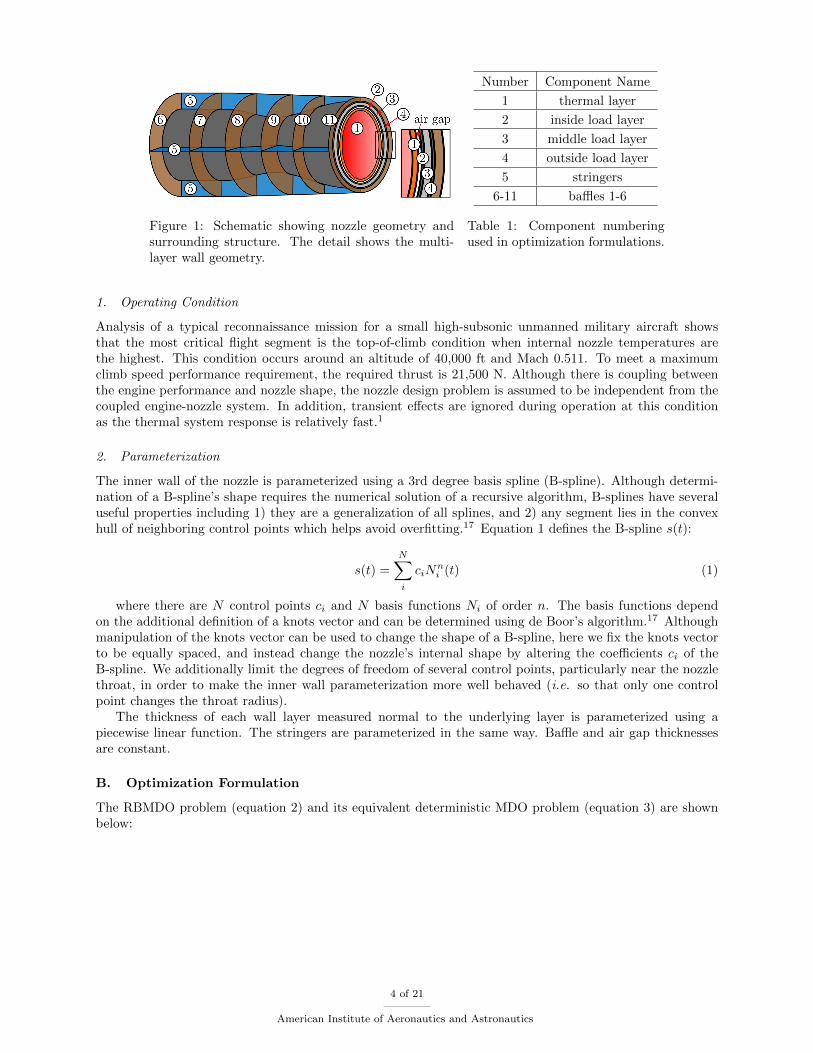
Figure 1: Schematic showing nozzle geometry andsurrounding structure. The detail shows the multi-layer wall geometry.

Number Component Name

1 thermal layer

2 inside load layer

3 middle load layer

4 outside load layer

5 stringers

6-11 baffles 1-6

Table 1: Component numberingused in optimization formulations.

1. Operating Condition

Analysis of a typical reconnaissance mission for a small high-subsonic unmanned military aircraft showsthat the most critical flight segment is the top-of-climb condition when internal nozzle temperatures arethe highest. This condition occurs around an altitude of 40,000 ft and Mach 0.511. To meet a maximumclimb speed performance requirement, the required thrust is 21,500 N. Although there is coupling betweenthe engine performance and nozzle shape, the nozzle design problem is assumed to be independent from thecoupled engine-nozzle system. In addition, transient effects are ignored during operation at this conditionas the thermal system response is relatively fast.1

2. Parameterization

The inner wall of the nozzle is parameterized using a 3rd degree basis spline (B-spline). Although determi-nation of a B-spline’s shape requires the numerical solution of a recursive algorithm, B-splines have severaluseful properties including 1) they are a generalization of all splines, and 2) any segment lies in the convexhull of neighboring control points which helps avoid overfitting.17 Equation 1 defines the B-spline s(t):

s(t) =

N∑i

ciNni (t) (1)

where there are N control points ci and N basis functions Ni of order n. The basis functions dependon the additional definition of a knots vector and can be determined using de Boor’s algorithm.17 Althoughmanipulation of the knots vector can be used to change the shape of a B-spline, here we fix the knots vectorto be equally spaced, and instead change the nozzle’s internal shape by altering the coefficients ci of theB-spline. We additionally limit the degrees of freedom of several control points, particularly near the nozzlethroat, in order to make the inner wall parameterization more well behaved (i.e. so that only one controlpoint changes the throat radius).

The thickness of each wall layer measured normal to the underlying layer is parameterized using apiecewise linear function. The stringers are parameterized in the same way. Baffle and air gap thicknessesare constant.

B. Optimization Formulation

The RBMDO problem (equation 2) and its equivalent deterministic MDO problem (equation 3) are shownbelow:

4 of 21


RBMDO Formulation:

minimizex∈<62

E[M(x, ξ)]

s.t. P [F (x, ξ) ≤ 21500] ≤ 10−7

P [m1 (T2(x, ξ)/Tmax,2) > 1] ≤ 10−7

P [m2 (S1(σ1(x, ξ))) > 1] ≤ 10−7

P [m3 (S2(σ2(x, ξ))) > 1] ≤ 10−7

P [m4 (S3(σ3(x, ξ))) > 1] ≤ 10−7

P [m5 (S4(σ4(x, ξ))) > 1] ≤ 10−7

P [m6 (S5(σ5(x, ξ))) > 1] ≤ 10−7

P [m7 (S6(σ6(x, ξ))) > 1] ≤ 10−7

P [m8 (S7(σ7(x, ξ))) > 1] ≤ 10−7

P [m9 (S8(σ8(x, ξ))) > 1] ≤ 10−7

P [m10 (S9(σ9(x, ξ))) > 1] ≤ 10−7

P [m11 (S10(σ10(x, ξ))) > 1] ≤ 10−7

P [m12 (S11(σ11(x, ξ))) > 1] ≤ 10−7

Ax ≤ bl ≤ x ≤ uξ ∈ <40

(2)

Deterministic MDO Formulation:

minimizex∈<62

M(x, µξ)

s.t. F (x, µξ) > 21500

m1 (T2(x, µξ)/Tmax,2) ≤ 1

m2 (S1(σ1(x, µξ))) ≤ 1

m3 (S2(σ2(x, µξ))) ≤ 1

m4 (S3(σ3(x, µξ))) ≤ 1

m5 (S4(σ4(x, µξ))) ≤ 1

m6 (S5(σ5(x, µξ))) ≤ 1

m7 (S6(σ6(x, µξ))) ≤ 1

m8 (S7(σ7(x, µξ))) ≤ 1

m9 (S8(σ8(x, µξ))) ≤ 1

m10 (S9(σ9(x, µξ))) ≤ 1

m11 (S10(σ10(x, µξ))) ≤ 1

m12 (S11(σ11(x, µξ))) ≤ 1

Ax ≤ bl ≤ x ≤ uξ ∈ <40

(3)

where x are deterministic design variables, ξ are random parameters with mean µξ = E[ξ], M(x, ξ) is themass of the nozzle, F (x, ξ) is the thrust, T2(x, ξ) is the temperature in the inside load layer, and Si(σi(x, ξ))is the stress failure criterion for nozzle component i where σi(x, ξ) is the stress field in component i. Ax ≤ bis a set of linear constraints and l and u are lower and upper bounds on the design variables, respectively.Refer to table 1 for the mapping between component name and component number.

The problem formulations above only contain one temperature constraint since temperature monotoni-cally decreases radially outward from the inner wall. Since the thermal layer is in direct contact with fluid,altering the nozzle shape will not change its maximum temperature due to the prescribed inlet stagnationtemperature. Instead, the temperature constraint is more appropriately placed on the inside load layer whichhas the next greatest temperatures.

Since temperature and stress are fields, a modified P-norm function m(z) is used to smoothly approximatea maximum of the field z as shown in equation 4.18 Based on numerical experiments a value of p = 10 isneither too conservative or relaxed. Kresselmeier-Steinhauser functions may also be used for the samepurpose; however they result in more conservative approximations.19

m(z) =

(1

N

N∑i

zpi

) 1p

(4)

In practice, solving the RBMDO problem above is difficult for several reasons including its large dimen-sion and the need to resolve small tail probabilities in the chance constraints. Thus, dimension reductiontechniques and methods for estimating small tail probabilities are imperative.

Here dimension reduction is performed in the ad hoc engineering sense of fixing design variables andremoving constraints that are not important. The solution of the full equivalent deterministic optimizationproblem in equation 3 is used to guide the dimension reduction and determine which variables and constraintsare important. The 36 design variables which meet their lower bounds at the solution of the deterministicoptimization are chosen to be fixed at their lower bounds for the reliable optimization problem. Thesevariables correspond to the thicknesses of components 1-11 in the nozzle, but not the thickness of the airgap. In addition, the last 7 stress failure criteria constraints are found to be very far from their bounds atall iterates during the deterministic optimization and are therefore removed from the reliable optimizationproblem. The need for estimating small tail probabilities is also mitigated by relaxing the probability levelin the chance constraints to 10−2. Lastly, the objective function has been replaced by M(x,E[ξ]) which

5 of 21


is easier to calculate and a good approximation of E[M(x, ξ)] (in our case, to within milligrams of mass).Equation 5 shows the reduced reliable optimization problem.

In addition, the RBMDO problem is normalized and reformulated in the spirit of a Performance MeasureApproach (PMA) prior to its solution. A PMA formulation constrains a response level of a CDF given aprobability level as opposed to the Reliability Index Approach (RIA) which constrains a probability levelof a CDF given a response level. Tu et al have shown that the PMA formulation is better-posed than anRIA formulation in certain cases, namely for inactive chance constraints.20 Equation 6 shows the scaledand reformulated optimization problem. The reformulation approach in equation 6 is not exactly PMAsince random variables are not mapped to a standard space and the generalized reliability index is not used,however it still benefits from constraints that are always well-defined.

Reduced RBMDO Formulation:

minimizex∈<26

M(x,E[ξ])

s.t. P [F (x, ξ) ≤ 21500] ≤ 10−2

P [m1 (T2(x, ξ)/Tmax,2) > 1] ≤ 10−2

P [m2 (S1(σ1(x, ξ))) > 1] ≤ 10−2

P [m3 (S2(σ2(x, ξ))) > 1] ≤ 10−2

P [m4 (S3(σ3(x, ξ))) > 1] ≤ 10−2

P [m5 (S4(σ4(x, ξ))) > 1] ≤ 10−2

Ax ≤ bl ≤ x ≤ uξ ∈ <40

(5)

PMA Reformulation:

minimizex∈<26

γM(x,E[ξ])

s.t. αF (x) ≤ 0

αT2(x) ≤ 0

αS1(x) ≤ 0

αS2(x) ≤ 0

αS3(x) ≤ 0

αS4(x) ≤ 0

Ax ≤ bl ≤ x ≤ uξ ∈ <40

(6)

where γ is a scaling coefficient for the mass, and αZ(x) is the normalized equivalent chance constraintformulated in the style of PMA. For example, for thrust:

αF (x) = 1−F−1F (10−2)

21500(7)

where F−1F is the inverse CDF for thrust. Similar reformulations are made for the temperature constraint

using m1 (T2(x, ξ)/Tmax,2) and the 4 stress failure criteria constraints using mi+1 (Si(σi(x, ξ))) , i ∈ 1 . . . 4.

1. Design Variables x

The full formulation (equations 2 and 3) uses 62 deterministic design variables x. 21 correspond to theaxial and radial coordinates of control points ci in the inner wall B-spline. 24 correspond to the breaklocations and thicknesses of each of the 4 material layers. 1 corresponds to the thickness of the air gap.6 correspond to the stringer thickness at each break location and 10 correspond to baffle axial positionsand thicknesses. The bounds for design variables governing thicknesses are determined by the minimumand maximum manufacturable material thicknesses. Bounds for other design variables are determined to be+/-20% of the value for the baseline nozzle shape.

The reduced formulation (equations 5 and 6) has 26 deterministic design variables x where all designvariables related to thickness have been removed, with the exception of the air gap thickness.

2. Random Parameters ξ

The problem considers 40 random parameters related to the material properties (35), atmospheric conditions(2), inlet conditions (2), and heat transfer (1). In particular, the atmospheric temperature and pressure,and inlet stagnation temperature and pressure are considered to be random. In addition, the heat transfercoefficient from the exterior surface of the nozzle to ambient conditions is considered to be random. Allparameters are considered to be independent.

Probability distributions for each random parameter are estimated using a variety of techniques. Forthe atmospheric conditions, mean values were taken from the 1970 U.S. Standard Atmosphere and varianceswere estimated from historical data provided at 60N under the assumption of a log-normal distribution.21

6 of 21


For the inlet conditions, uncertainties in engine parameters were propagated through a F100-PW-220 enginemodel (similar to that from reference 23) using simple Monte Carlo (SMC) and a log-normal distributionwas fit to the resulting histograms. Data used to construct the engine model was taken from a variety ofsources.22–24 The heat transfer coefficient was estimated by fitting a log-normal distribution to a histogramformed by SMC forward propagation of material and geometric uncertainties in a linear thermal resistanceheat transfer model. Distributions for the material properties were estimated from experimental data whenavailable.25–29 Otherwise, expert knowledge was used to determine variances or possible ranges.

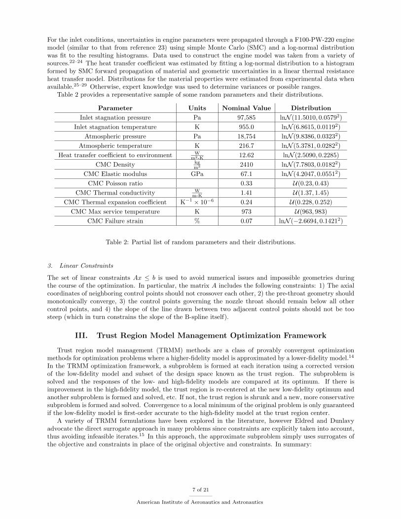
Table 2 provides a representative sample of some random parameters and their distributions.

Parameter Units Nominal Value Distribution

Inlet stagnation pressure Pa 97,585 lnN (11.5010, 0.05792)

Inlet stagnation temperature K 955.0 lnN (6.8615, 0.01192)

Atmospheric pressure Pa 18,754 lnN (9.8386, 0.03232)

Atmospheric temperature K 216.7 lnN (5.3781, 0.02822)

Heat transfer coefficient to environment Wm2-K 12.62 lnN (2.5090, 0.2285)

CMC Density kgm3 2410 lnN (7.7803, 0.01822)

CMC Elastic modulus GPa 67.1 lnN (4.2047, 0.05512)

CMC Poisson ratio 0.33 U(0.23, 0.43)

CMC Thermal conductivity Wm-K 1.41 U(1.37, 1.45)

CMC Thermal expansion coefficient K−1 × 10−6 0.24 U(0.228, 0.252)

CMC Max service temperature K 973 U(963, 983)

CMC Failure strain % 0.07 lnN (−2.6694, 0.14212)

Table 2: Partial list of random parameters and their distributions.

3. Linear Constraints

The set of linear constraints Ax ≤ b is used to avoid numerical issues and impossible geometries duringthe course of the optimization. In particular, the matrix A includes the following constraints: 1) The axialcoordinates of neighboring control points should not crossover each other, 2) the pre-throat geometry shouldmonotonically converge, 3) the control points governing the nozzle throat should remain below all othercontrol points, and 4) the slope of the line drawn between two adjacent control points should not be toosteep (which in turn constrains the slope of the B-spline itself).

III. Trust Region Model Management Optimization Framework

Trust region model management (TRMM) methods are a class of provably convergent optimizationmethods for optimization problems where a higher-fidelity model is approximated by a lower-fidelity model.14

In the TRMM optimization framework, a subproblem is formed at each iteration using a corrected versionof the low-fidelity model and subset of the design space known as the trust region. The subproblem issolved and the responses of the low- and high-fidelity models are compared at its optimum. If there isimprovement in the high-fidelity model, the trust region is re-centered at the new low-fidelity optimum andanother subproblem is formed and solved, etc. If not, the trust region is shrunk and a new, more conservativesubproblem is formed and solved. Convergence to a local minimum of the original problem is only guaranteedif the low-fidelity model is first-order accurate to the high-fidelity model at the trust region center.

A variety of TRMM formulations have been explored in the literature, however Eldred and Dunlavyadvocate the direct surrogate approach in many problems since constraints are explicitly taken into account,thus avoiding infeasible iterates.15 In this approach, the approximate subproblem simply uses surrogates ofthe objective and constraints in place of the original objective and constraints. In summary:

7 of 21


Original Formulation:

minimizex

f(x)

s.t. g(x) ≤ 0

Ax ≤ bl ≤ x ≤ u

k-th Subproblem Formulation:

minimizex

fk(x)

s.t. gk(x) ≤ 0

Ax ≤ b∥∥x− xkc∥∥∞ ≤ ∆k

l ≤ x ≤ u

where f(x) denotes the objective function, g(x) denotes the nonlinear constraints, Ax ≤ b denotes thelinear constraints, and l and u are the lower and upper bounds on the design variables x. In the subproblemformulation, fk(x) is used to denote the corrected surrogate function of the original objective for the k-thsubproblem and likewise for gk(x). Note the additional restriction on the design space through the use of atrust region constraint where the center of the trust region is xc and it has size ∆k.

A. Low-fidelity Correction

First-order and second-order multiplicative and additive corrections have been investigated in the litera-ture.15,30 Here, we use a first-order additive correction for simplicity to match the low-fidelity model’sobjective and constraint responses flo, glo and gradients to the high-fidelity model’s responses fhi, ghi andgradients at the center of the trust region xc. The k-th additive correction δk is determined as:30

δk = fhi(xkc )− flo(xkc ) (8)

Thus, the first-order corrected surrogate model f(x) is:

f(x) = flo(x) + δk +(∇δk

)T(x− xc) (9)

B. Iterate Acceptance

Two methods are commonly used to accept or reject the optimum of the subproblem for a given TRMMiteration. One method forms a trust region ratio from a merit function involving the low- and high-fidelityobjective and constraint values14 (see section C). Another method, and the one used here, is the filtermethod.15 In this method, the iterate is accepted if either f(x∗) < f (i) or v(x∗) < v(i) for all i in the filter,that is for all previously recorded values of f and v. v(x) is a measure of the constraint violation; here weuse v(x) = ‖g(x)‖2 ∀g(x) > 0.

C. Trust-Region Update

A merit function is used to form a trust region ratio to assess the quality of the low-fidelity approximation.The trust region ratio ρ is defined in equation 10.15 As can be seen, ρ ≈ 1 if the low-fidelity approximatesthe high-fidelity model well. For small values of ρ, the trust region is shrunk (ρ < 0.25), for intermediateor large values it retains the same size (0.25 ≤ ρ ≤ 0.75 and ρ > 1.25), and for values close to 1 it expands(0.75 ≤ ρ ≤ 1.25).

ρk =Φhi(xc)− Φhi(x

∗)

Φlo(xc)− Φlo(x∗)(10)

where Φ(x) is the merit function. Proposed merit functions have included the Lagrangian, augmentedLagrangian, and penalty-type functions.15 A penalty-type merit function is used here since it is easilyimplemented:

Φ(x, rp) = f(x) + rpg+(x)T g+(x) (11)

where g+(x) is the set of active nonlinear constraints, and rp = e(k+offset)/10 as used by Eldred andDunlavy.15

8 of 21


IV. Surrogate Construction

When model evaluations are expensive, surrogate models may be required for stochastic quantities ofinterest in order to make the calculation of statistics tractable. In addition, many model responses are afunction of both deterministic and random variables. In this case, separating the complex function governingthe model response into deterministic and random components can additionally simplify the calculation ofstatistics and overall optimization process when embedded in a TRMM framework.

Our approach uses anchored decomposition and polynomial chaos expansions to construct a low-fidelitysurrogate model for each chance constraint in equation 6. Anchored decomposition is used to first separatethe contribution of the deterministic design variables and random parameters to the function response.A polynomial chaos expansion is then used to further approximate the stochastic term in the anchoreddecomposition.

A. Anchored Decomposition

Decomposition techniques approximate a function of several variables by a sum or product of simpler func-tions of which anchored decomposition is the simplest form. Another popular method is the ANOVA (Analy-sis of Variance) decomposition, but as this approach requires integrals whose numerical computation requiresadditional sampling of the original function it is not used here.12

In anchored decomposition a function is decomposed into a sum of terms, where each term is a projectionof the function onto a subset of the function’s variables.12 For the case of a function consisting of two setsof variables x and ξ, the function is separated in the following way:

f(x, ξ) + f(x0, ξ0)− f(x0, ξ)− f(x, ξ0) = 0 (12)

where (x0, ξ0) is a set of fixed values, i.e. the anchor. Note that equation 12 is true if one fixes x = x0 forall ξ, and is likewise true if one fixes ξ = ξ0 for all x. As x and ξ change together, the following approximationcan be written for the function f , so long as x is close to x0, ξ is close to ξ0 and the function is well-behaved:

f(x, ξ) ≈ f(x0, ξ) + f(x, ξ0)− f(x0, ξ0) (13)

In general, anchored decomposition can be applied to more than 2 sets of variables, however determiningwhich variables belong to which sets is not always clear. The anchored decomposition approximation canbe expected to be less accurate away from the anchor when correlated variables have been separated intodifferent sets. We make the intuitive choice of separating deterministic x from random ξ. In many physicalproblems, variables may also already be classified as belonging to certain (typically correlated) groups.

B. Polynomial Chaos Expansions

The polynomial chaos expansion (PCE) is a classical uncertainty quantification method which approximatesa function of random variables by a series of mutually orthogonal polynomials. Although the expansion canbe performed for deterministic and random variables, it has traditionally been used with random variables,beginning with the pioneering work of Ghanem and Spanos.31 Further developments revealed a connectionbetween the types of random variables in the function and corresponding orthogonal polynomial baseswhich give optimal convergence of polynomial coefficients. This expanded approach is known as generalizedpolynomial chaos (gPC).10

In gPC, the polynomial basis for the expansion is selected a priori from the Askey scheme of polynomi-als. For example, for Gaussian random variables the Hermite polynomials are used and for uniform randomvariables the Legendre polynomials are used.10 In addition, mixed random variables can be easily accom-modated by mixing the polynomial basis since orthogonality properties are still preserved when orthogonalpolynomials are used.32 A function f(ξ) can be expanded as:

f(ξ) ≈ fPCE(ξ) =

Q∑i=1

aiΨi(ξ) (14)

where Ψi(ξ) is the i-th basis function, ai is the i-th coefficient, and the expansion is approximate since ithas been truncated to include Q terms. The difficulty of efficiently completing the approximation in equation14 lies in the calculation of the coefficients ai which is described below in section 1.

9 of 21


Polynomial chaos methods can be separated into intrusive and non-intrusive approaches. Intrusive ap-proaches require embedding the expansion in equation 14 directly into the governing equations and solving anew expanded and coupled system of equations which may be difficult in practice. The non-intrusive methodis more more easily implemented for existing models as it simply samples the function f(ξ) at quadraturepoints to estimate the the coefficients and thereby builds the expansion. Both approaches introduce trunca-tion error, but the non-intrusive approach also introduces an error due to the use of quadrature.

1. Calculation of Coefficients

In the non-intrusive approach, the coefficients ai can be calculated using a pseudo-spectral projection processas shown in equation 15:32

ai =1

〈Ψ2i (ξ)〉

∫Ω

fPCE(ξ)Ψi(ξ)w(ξ)dξ (15)

where the inner product 〈Ψi(ξ)〉 can be calculated a priori and w(ξ) is the weight function correspondingto polynomial basis Ψi(ξ). The multidimensional integral over Ω, the space spanned by all random variablesin ξ, can be approximated using quadrature, of which several techniques have been used including tensorproduct quadrature, cubature, and sparse grids.33 For a small number of variables, full tensor productquadrature works well, but for higher dimensions, full tensor product quadrature is too expensive and asparse grid approach is more tractable although less accurate for non-smooth functions.32,33 In this work,we use sparse grid quadrature.

Sparse grid quadrature requires evaluation of the integrand at a relatively small number of points whichcollectively are called the sparse grid. The sparse grid and its associated quadrature weights are determinedvia a desired quadrature rule (Clenshaw-Curtis, Gauss, etc.) and a level ` which determines the sparsity ofthe grid. A sparse grid is formed by extending Smolyak’s 1-D interpolation formula to multiple dimensions.The Smolyak isotropic interpolation formula A(`, n) is a linear combination of product formulas and can bewritten in the form found in equation 16:32,33

A(`, n) =∑

`+1≤|i|≤`+n

(−1)`+n−|i|

(n− 1

`+ n− |i|

)(U i1 ⊗ . . .⊗ U in) (16)

where ` is the level of the sparse grid, n is the number of variables, i = (i1, . . . , in), and U ij is the 1-Dinterpolant over the space spanned by the ij-th variable. As can be seen in equation 16, the 1-D interpolantsU i1 . . .U in need only be evaluated for `+ 1 ≤ i1 + . . .+ in ≤ `+n, i.e. at a small subset of points H(`, n). Inaddition, sparse grids may also be nested so that H(`, n) ⊂ H(`+ 1, n), thereby allowing reuse of grid pointsfor efficiency.32 When using a level 1 sparse grid (` = 1), the coefficients ai can be calculated using 2n + 1evaluations of the integrand. Level 2 nested sparse grid quadrature requires 2n2 + 2n+ 1 evaluations insteadwhen Chebyshev abscissas are used. Although sparse grid makes evaluation of the integral in equation 15more tractable, for large numbers of variables and higher accuracy (i.e. higher grid level), evaluation ofcoefficients may still be costly.

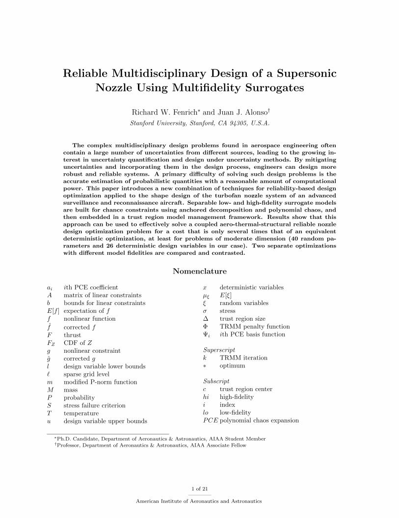
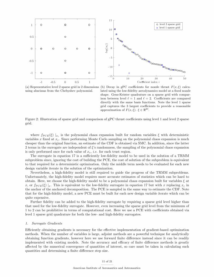
In this work, gPC coefficients are evaluated with Genz-Keister quadrature on a level 1 sparse grid asimplemented in the open-source Dakota software package.34 Figure 2a shows a level 2 sparse grid in 2dimensions. Figure 2 compares the decay in polynomial coefficients for the approximation of nozzle thrustusing a level 1 and level 2 sparse grid.

C. Surrogate for Chance Constraints

As shown previously, a chance constraint can be reformulated using PMA such that its evaluation dependson evaluating the inverse CDF at the desired probability level (equation 7). Thus we seek a method forapproximating the inverse CDF (or CDF) for a random field f(x, ξ) which is dependent on both deterministicvariables x and random parameters ξ.

First, an anchored decomposition approximation is made for the random field as shown in equation 13where the anchor (x0, ξ0) is taken to be (xc, E[ξ]) where xc is the center of a trust region. Next, the randomcomponent of the resulting approximation is further approximated with a PCE as shown in equation 17:

f(x, ξ) ≈ fPCE(ξ) |xc +f(x,E[ξ])− f(xc, E[ξ]) (17)

10 of 21


-1 -0.5 0 0.5 1

-1

-0.5

0.5

0

1

(a) Representative level 2 sparse grid in 2 dimensionsusing abscissas from the Chebyshev polynomial.

0 10 20 30 40 50

Coecient index i

- 15

- 10

- 5

10

15

log(|ai|)

5

0

level 2 sparse grid

level 1 sparse grid

(b) Decay in gPC coefficients for nozzle thrust F (x, ξ) calcu-lated using the low-fidelity aerodynamics model at a fixed nozzleshape. Genz-Keister quadrature on a sparse grid with compar-ison between level ` = 1 and ` = 2. Coefficients are compareddirectly with the same basis functions. Note the level 1 sparsegrid captures the 3 largest coefficients to provide a reasonableapproximation of F (x, ξ). ξ ∈ <40.

Figure 2: Illustration of sparse grid and comparison of gPC thrust coefficients using level 1 and level 2 sparsegrid.

where fPCE(ξ) |xc is the polynomial chaos expansion built for random variables ξ with deterministicvariables x fixed at xc. Since performing Monte Carlo sampling on the polynomial chaos expansion is muchcheaper than the original function, an estimate of the CDF is obtained via SMC. In addition, since the latter2 terms in the surrogate are independent of ξ’s randomness, the sampling of the polynomial chaos expansionis only performed once for each value of xc, i.e. for each trust region.

The surrogate in equation 17 is a sufficiently low-fidelity model to be used in the solution of a TRMMsubproblem since, ignoring the cost of building the PCE, the cost of solution of the subproblem is equivalentto that required for a deterministic optimization. Only the middle term needs to be evaluated for each newdesign variable iterate in the solution of the optimization.

Nevertheless, a high-fidelity model is still required to guide the progress of the TRMM subproblems.Unfortunately, the high-fidelity model requires more accurate estimates of statistics which can be hard toobtain. Here, we choose the high-fidelity model to be a polynomial chaos expansion built for variables ξ atx, or fPCE(ξ) |x. This is equivalent to the low-fidelity surrogate in equation 17 but with x replacing xc inthe anchor of the anchored decomposition. The PCE is sampled in the same way to estimate the CDF. Notethat for the high-fidelity model, a new PCE must be built for each new design variable iterate which can bequite expensive.

Further fidelity can be added to the high-fidelity surrogate by requiring a sparse grid level higher thanthat used for the low-fidelity surrogate. However, even increasing the sparse grid level from the minimum of1 to 2 can be prohibitive in terms of computational cost. Here we use a PCE with coefficients obtained vialevel 1 sparse grid quadrature for both the low- and high-fidelity surrogates.

1. Surrogate Gradients

Efficiently obtaining gradients is necessary for the effective implementation of gradient-based optimizationmethods. When the number of variables is large, adjoint methods are a powerful technique for analyticallyobtaining function gradients, however here we use forward finite difference instead since it can be readilyimplemented with existing models. Note the accuracy and efficacy of finite difference methods is greatlyaffected by the numerical convergence of quantities of interest, so care must be taken in calculating suchquantities and determining a finite difference step size.

11 of 21


Low-fidelity MDA

Quasi-1D aero analysis

FEMthermal analysis

FEMstructural analysis

wall temperature wall pressure

σi

stresses

T2

temperatureTi

temperatures

Fthrust

x, ξi

x, ξi x, ξi x, ξi

1D heattransferanalysis

wall temperature

stagnation temp. friction coef.

Aerothermal analysis

x, ξi

stagnation temp. friction coef.

x, ξi

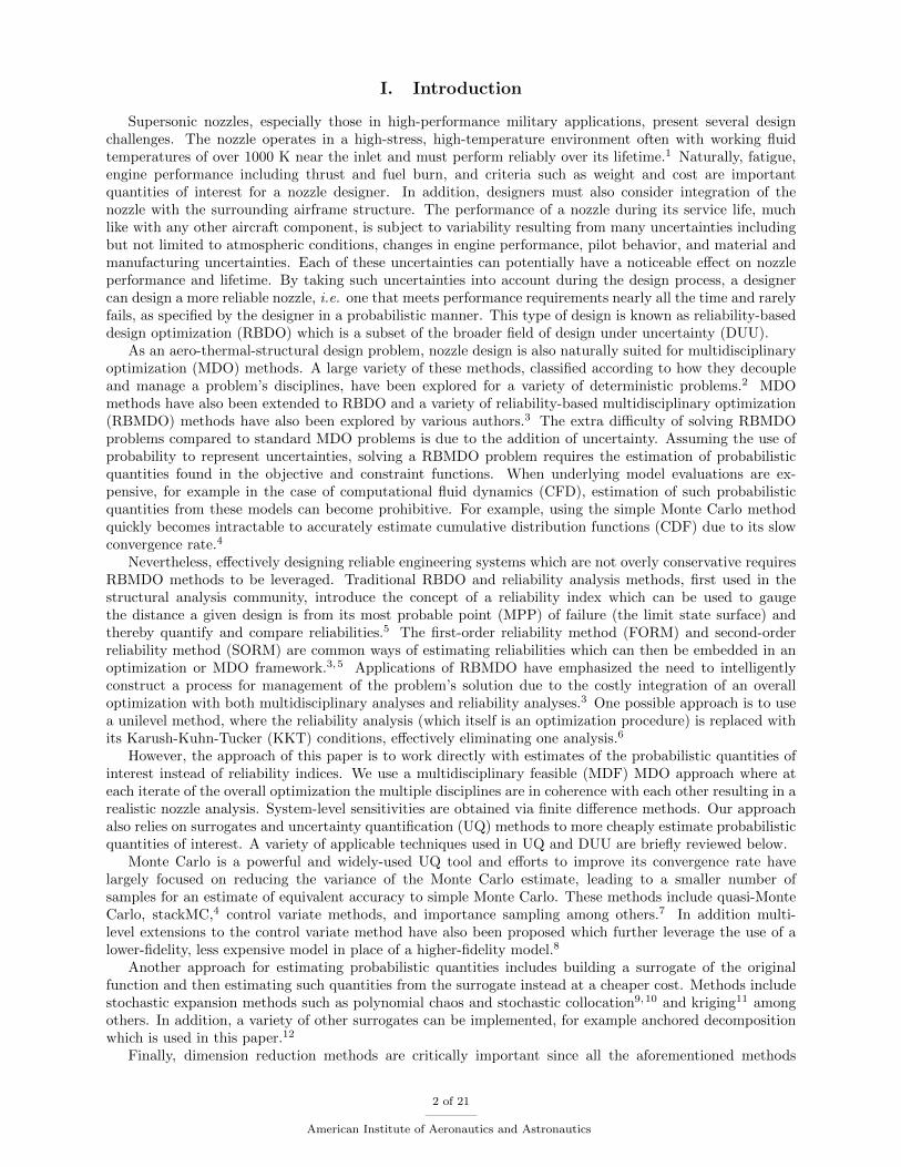
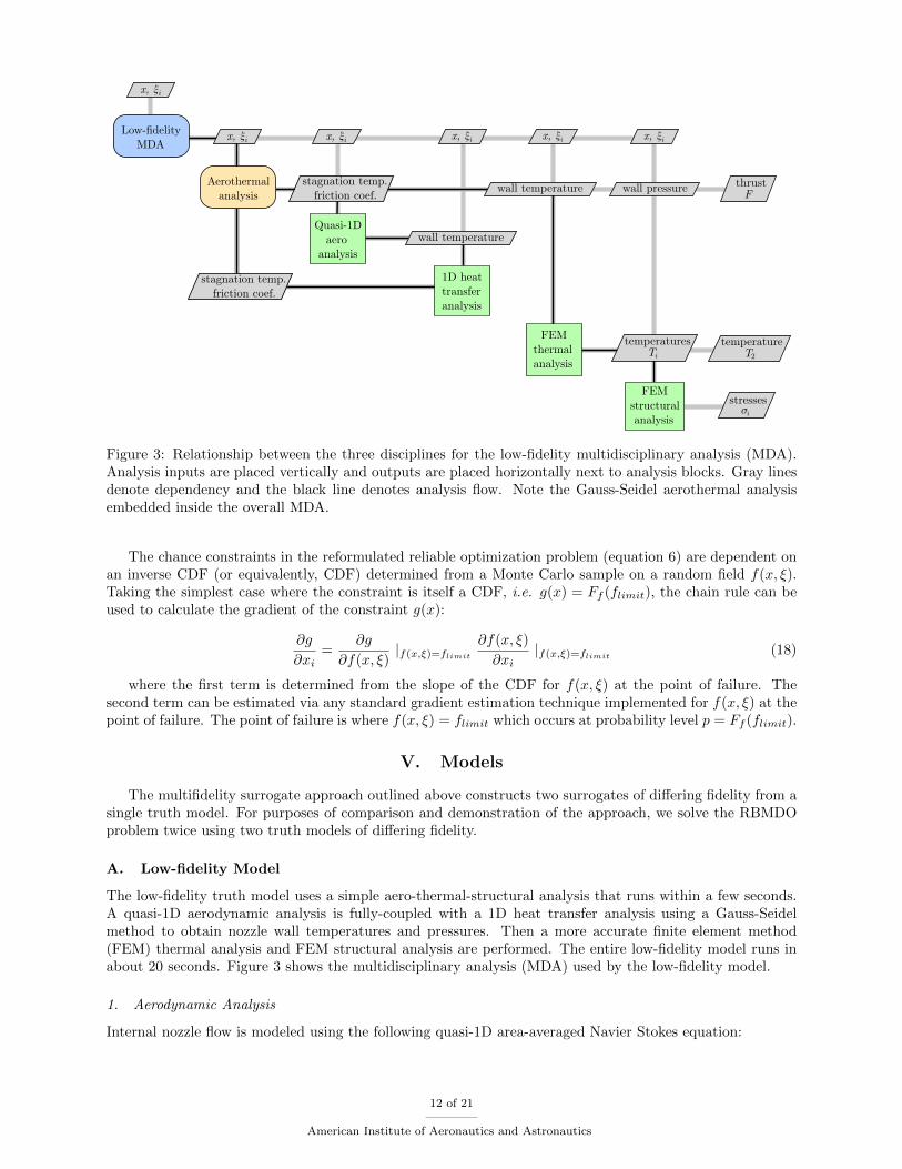
Figure 3: Relationship between the three disciplines for the low-fidelity multidisciplinary analysis (MDA).Analysis inputs are placed vertically and outputs are placed horizontally next to analysis blocks. Gray linesdenote dependency and the black line denotes analysis flow. Note the Gauss-Seidel aerothermal analysisembedded inside the overall MDA.

The chance constraints in the reformulated reliable optimization problem (equation 6) are dependent onan inverse CDF (or equivalently, CDF) determined from a Monte Carlo sample on a random field f(x, ξ).Taking the simplest case where the constraint is itself a CDF, i.e. g(x) = Ff (flimit), the chain rule can beused to calculate the gradient of the constraint g(x):

∂g

∂xi=

∂g

∂f(x, ξ)|f(x,ξ)=flimit

∂f(x, ξ)

∂xi|f(x,ξ)=flimit (18)

where the first term is determined from the slope of the CDF for f(x, ξ) at the point of failure. Thesecond term can be estimated via any standard gradient estimation technique implemented for f(x, ξ) at thepoint of failure. The point of failure is where f(x, ξ) = flimit which occurs at probability level p = Ff (flimit).

V. Models

The multifidelity surrogate approach outlined above constructs two surrogates of differing fidelity from asingle truth model. For purposes of comparison and demonstration of the approach, we solve the RBMDOproblem twice using two truth models of differing fidelity.

A. Low-fidelity Model

The low-fidelity truth model uses a simple aero-thermal-structural analysis that runs within a few seconds.A quasi-1D aerodynamic analysis is fully-coupled with a 1D heat transfer analysis using a Gauss-Seidelmethod to obtain nozzle wall temperatures and pressures. Then a more accurate finite element method(FEM) thermal analysis and FEM structural analysis are performed. The entire low-fidelity model runs inabout 20 seconds. Figure 3 shows the multidisciplinary analysis (MDA) used by the low-fidelity model.

1. Aerodynamic Analysis

Internal nozzle flow is modeled using the following quasi-1D area-averaged Navier Stokes equation:

12 of 21


High-fidelity MDA

Euler CFD analysis

FEMthermal analysis

FEMstructural analysis

wall temperature wall pressure

σi

stresses

T2

temperatureTi

temperatures

Fthrust

x, ξi

x, ξi x, ξi x, ξi

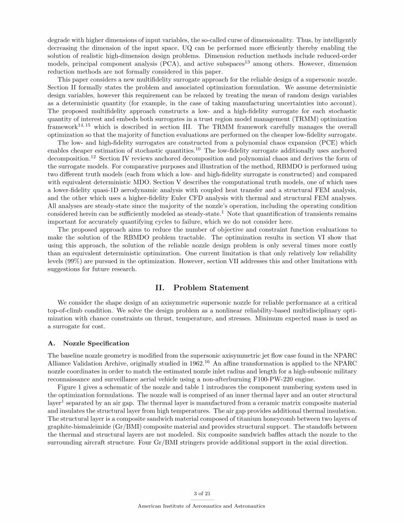
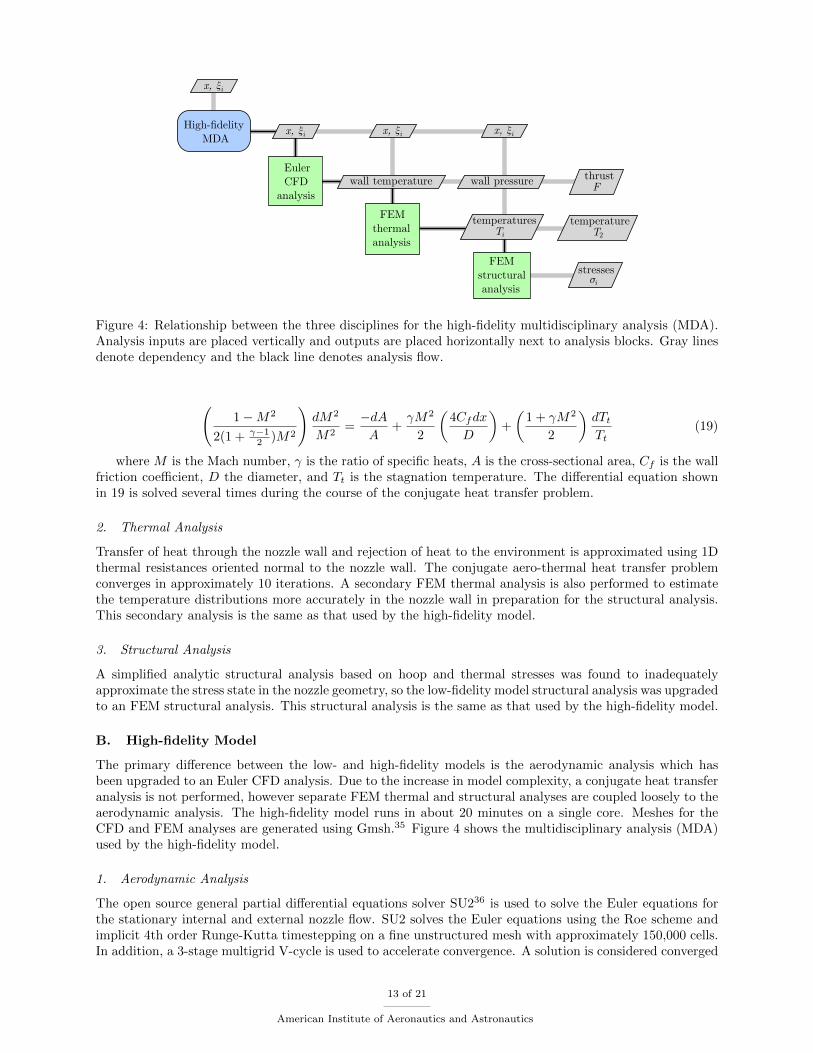
Figure 4: Relationship between the three disciplines for the high-fidelity multidisciplinary analysis (MDA).Analysis inputs are placed vertically and outputs are placed horizontally next to analysis blocks. Gray linesdenote dependency and the black line denotes analysis flow.

(1−M2

2(1 + γ−12 )M2

)dM2

M2=−dAA

+γM2

2

(4Cfdx

D

)+

(1 + γM2

2

)dTtTt

(19)

where M is the Mach number, γ is the ratio of specific heats, A is the cross-sectional area, Cf is the wallfriction coefficient, D the diameter, and Tt is the stagnation temperature. The differential equation shownin 19 is solved several times during the course of the conjugate heat transfer problem.

2. Thermal Analysis

Transfer of heat through the nozzle wall and rejection of heat to the environment is approximated using 1Dthermal resistances oriented normal to the nozzle wall. The conjugate aero-thermal heat transfer problemconverges in approximately 10 iterations. A secondary FEM thermal analysis is also performed to estimatethe temperature distributions more accurately in the nozzle wall in preparation for the structural analysis.This secondary analysis is the same as that used by the high-fidelity model.

3. Structural Analysis

A simplified analytic structural analysis based on hoop and thermal stresses was found to inadequatelyapproximate the stress state in the nozzle geometry, so the low-fidelity model structural analysis was upgradedto an FEM structural analysis. This structural analysis is the same as that used by the high-fidelity model.

B. High-fidelity Model

The primary difference between the low- and high-fidelity models is the aerodynamic analysis which hasbeen upgraded to an Euler CFD analysis. Due to the increase in model complexity, a conjugate heat transferanalysis is not performed, however separate FEM thermal and structural analyses are coupled loosely to theaerodynamic analysis. The high-fidelity model runs in about 20 minutes on a single core. Meshes for theCFD and FEM analyses are generated using Gmsh.35 Figure 4 shows the multidisciplinary analysis (MDA)used by the high-fidelity model.

1. Aerodynamic Analysis

The open source general partial differential equations solver SU236 is used to solve the Euler equations forthe stationary internal and external nozzle flow. SU2 solves the Euler equations using the Roe scheme andimplicit 4th order Runge-Kutta timestepping on a fine unstructured mesh with approximately 150,000 cells.In addition, a 3-stage multigrid V-cycle is used to accelerate convergence. A solution is considered converged

13 of 21


0.03

0.87

1.72

2.56

3.41

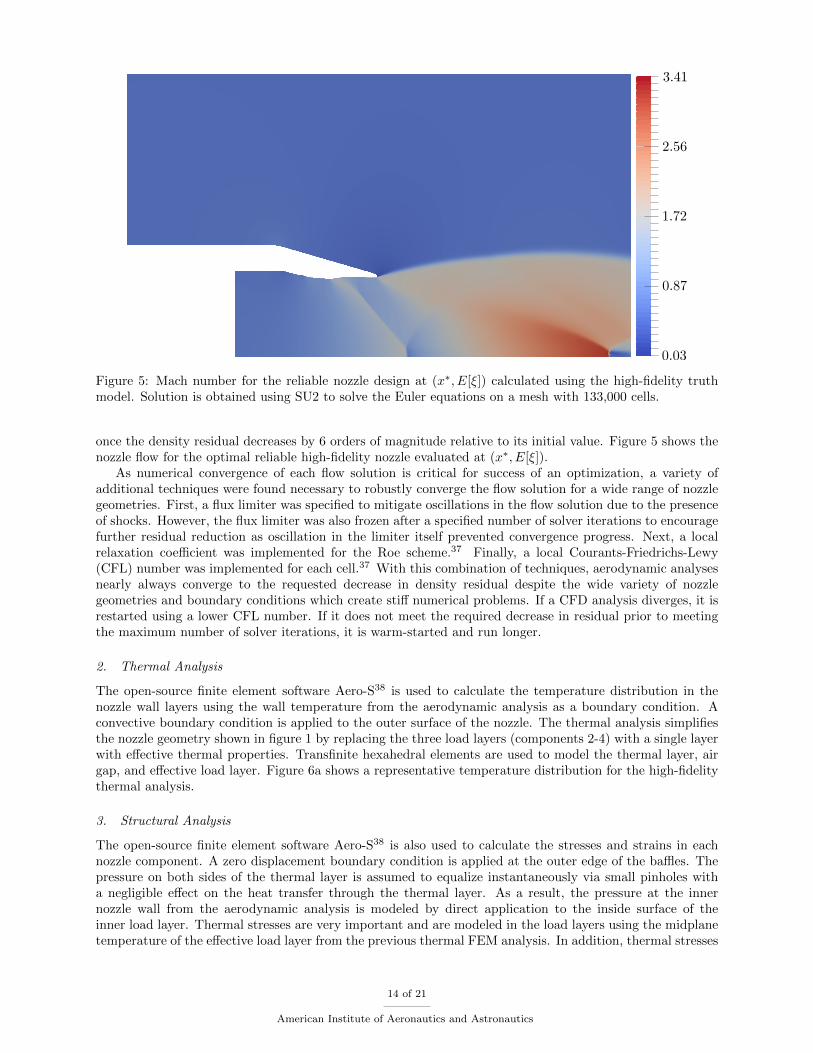
Figure 5: Mach number for the reliable nozzle design at (x∗, E[ξ]) calculated using the high-fidelity truthmodel. Solution is obtained using SU2 to solve the Euler equations on a mesh with 133,000 cells.

once the density residual decreases by 6 orders of magnitude relative to its initial value. Figure 5 shows thenozzle flow for the optimal reliable high-fidelity nozzle evaluated at (x∗, E[ξ]).

As numerical convergence of each flow solution is critical for success of an optimization, a variety ofadditional techniques were found necessary to robustly converge the flow solution for a wide range of nozzlegeometries. First, a flux limiter was specified to mitigate oscillations in the flow solution due to the presenceof shocks. However, the flux limiter was also frozen after a specified number of solver iterations to encouragefurther residual reduction as oscillation in the limiter itself prevented convergence progress. Next, a localrelaxation coefficient was implemented for the Roe scheme.37 Finally, a local Courants-Friedrichs-Lewy(CFL) number was implemented for each cell.37 With this combination of techniques, aerodynamic analysesnearly always converge to the requested decrease in density residual despite the wide variety of nozzlegeometries and boundary conditions which create stiff numerical problems. If a CFD analysis diverges, it isrestarted using a lower CFL number. If it does not meet the required decrease in residual prior to meetingthe maximum number of solver iterations, it is warm-started and run longer.

2. Thermal Analysis

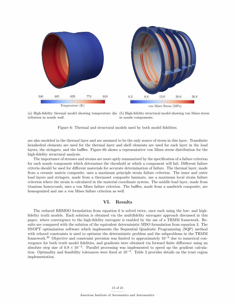
The open-source finite element software Aero-S38 is used to calculate the temperature distribution in thenozzle wall layers using the wall temperature from the aerodynamic analysis as a boundary condition. Aconvective boundary condition is applied to the outer surface of the nozzle. The thermal analysis simplifiesthe nozzle geometry shown in figure 1 by replacing the three load layers (components 2-4) with a single layerwith effective thermal properties. Transfinite hexahedral elements are used to model the thermal layer, airgap, and effective load layer. Figure 6a shows a representative temperature distribution for the high-fidelitythermal analysis.

3. Structural Analysis

The open-source finite element software Aero-S38 is also used to calculate the stresses and strains in eachnozzle component. A zero displacement boundary condition is applied at the outer edge of the baffles. Thepressure on both sides of the thermal layer is assumed to equalize instantaneously via small pinholes witha negligible effect on the heat transfer through the thermal layer. As a result, the pressure at the innernozzle wall from the aerodynamic analysis is modeled by direct application to the inside surface of theinner load layer. Thermal stresses are very important and are modeled in the load layers using the midplanetemperature of the effective load layer from the previous thermal FEM analysis. In addition, thermal stresses

14 of 21


340 485 629 774 919

Temperature (K)

(a) High-fidelity thermal model showing temperature dis-tribution in nozzle wall.

0.2 6.8 13.0 20.0 26.8

von Mises Stress (MPa)

(b) High-fidelity structural model showing von Mises stressin nozzle components.

Figure 6: Thermal and structural models used by both model fidelities.

are also modeled in the thermal layer and are assumed to be the only source of stress in this layer. Transfinitehexahedral elements are used for the thermal layer and shell elements are used for each layer in the loadlayers, the stringers, and the baffles. Figure 6b shows a representative von Mises stress distribution for thehigh-fidelity structural analysis.

The importance of stresses and strains are more aptly summarized by the specification of a failure criterionfor each nozzle component which determines the threshold at which a component will fail. Different failurecriteria should be used for different materials for accurate determination of failure. The thermal layer, madefrom a ceramic matrix composite, uses a maximum principle strain failure criterion. The inner and outerload layers and stringers, made from a thermoset composite laminate, use a maximum local strain failurecriterion where the strain is calculated in the material coordinate system. The middle load layer, made fromtitanium honeycomb, uses a von Mises failure criterion. The baffles, made from a sandwich composite, arehomogenized and use a von Mises failure criterion as well.

VI. Results

The reduced RBMDO formulation from equation 6 is solved twice, once each using the low- and high-fidelity truth models. Each solution is obtained via the multifidelity surrogate approach discussed in thispaper, where convergence to the high-fidelity surrogate is enabled by the use of a TRMM framework. Re-sults are compared with the solution of the equivalent deterministic MDO formulation from equation 3. TheSNOPT optimization software which implements the Sequential Quadratic Programming (SQP) methodwith relaxed constraints is used to optimize the deterministic problem and the subproblems in the TRMMframework.39 Objective and constraint precision was limited to approximately 10−6 due to numerical con-vergence for both truth model fidelities, and gradients were obtained via forward finite difference using anabsolute step size of 0.9 × 10−3. Parallel processing was implemented to speed up the gradient calcula-tion. Optimality and feasibility tolerances were fixed at 10−3. Table 3 provides details on the trust regionimplementation.

15 of 21


Approximate Subproblem direct

Merit function Φ(x) penalty

Low-fidelity Correction additive, 1st order

Acceptance Test filter method

Initial Size 0.016

Contract Threshold 0.25

Expand Threshold 0.75

Contraction Factor 0.25

Expansion Factor 1.5

Soft Convergence Limit 3

Convergence Tolerance 10−4

Constraint Tolerance 10−4

Table 3: Trust region parameters used for the solution of the RBMDO problem in equation 6.

A. Low-fidelity Design

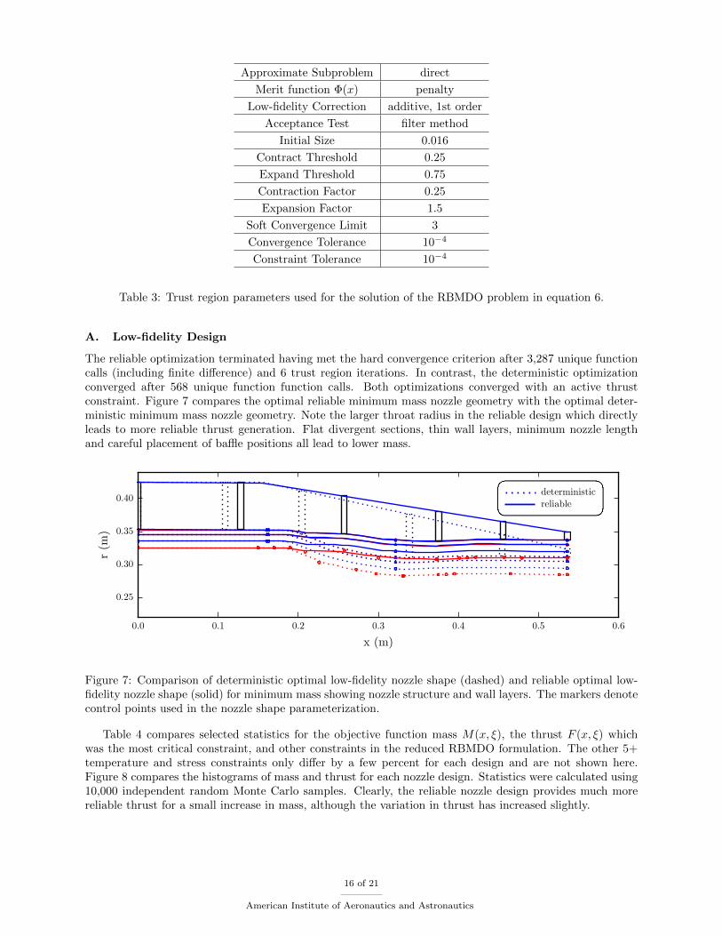
The reliable optimization terminated having met the hard convergence criterion after 3,287 unique functioncalls (including finite difference) and 6 trust region iterations. In contrast, the deterministic optimizationconverged after 568 unique function function calls. Both optimizations converged with an active thrustconstraint. Figure 7 compares the optimal reliable minimum mass nozzle geometry with the optimal deter-ministic minimum mass nozzle geometry. Note the larger throat radius in the reliable design which directlyleads to more reliable thrust generation. Flat divergent sections, thin wall layers, minimum nozzle lengthand careful placement of baffle positions all lead to lower mass.

0.0 0.1 0.2 0.3 0.4 0.5 0.6

x (m)

0.25

0.30

0.35

0.40

r (m

)

deterministicreliable

Figure 7: Comparison of deterministic optimal low-fidelity nozzle shape (dashed) and reliable optimal low-fidelity nozzle shape (solid) for minimum mass showing nozzle structure and wall layers. The markers denotecontrol points used in the nozzle shape parameterization.

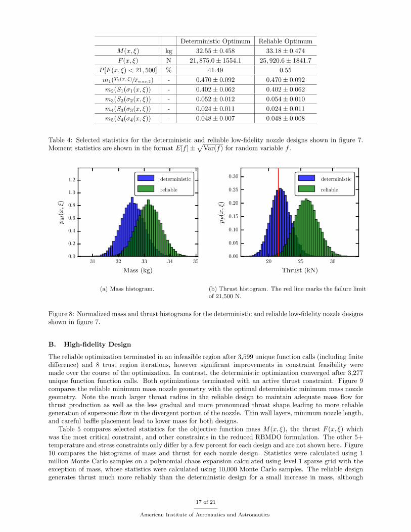
Table 4 compares selected statistics for the objective function mass M(x, ξ), the thrust F (x, ξ) whichwas the most critical constraint, and other constraints in the reduced RBMDO formulation. The other 5+temperature and stress constraints only differ by a few percent for each design and are not shown here.Figure 8 compares the histograms of mass and thrust for each nozzle design. Statistics were calculated using10,000 independent random Monte Carlo samples. Clearly, the reliable nozzle design provides much morereliable thrust for a small increase in mass, although the variation in thrust has increased slightly.

16 of 21


Deterministic Optimum Reliable Optimum

M(x, ξ) kg 32.55± 0.458 33.18± 0.474

F (x, ξ) N 21, 875.0± 1554.1 25, 920.6± 1841.7

P [F (x, ξ) < 21, 500] % 41.49 0.55

m1(T2(x, ξ)/Tmax,2) - 0.470± 0.092 0.470± 0.092

m2(S1(σ1(x, ξ)) - 0.402± 0.062 0.402± 0.062

m3(S2(σ2(x, ξ)) - 0.052± 0.012 0.054± 0.010

m4(S3(σ3(x, ξ)) - 0.024± 0.011 0.024± 0.011

m5(S4(σ4(x, ξ)) - 0.048± 0.007 0.048± 0.008

Table 4: Selected statistics for the deterministic and reliable low-fidelity nozzle designs shown in figure 7.Moment statistics are shown in the format E[f ]±

√Var(f) for random variable f .

31 32 33 34 35Mass (kg)

0.0

0.2

0.4

0.6

0.8

1.0

1.2

pM

(x,ξ

)

deterministic

reliable

(a) Mass histogram.

20 25 30Thrust (kN)

0.00

0.05

0.10

0.15

0.20

0.25

0.30

pF(x,ξ

)

deterministic

reliable

(b) Thrust histogram. The red line marks the failure limitof 21,500 N.

Figure 8: Normalized mass and thrust histograms for the deterministic and reliable low-fidelity nozzle designsshown in figure 7.

B. High-fidelity Design

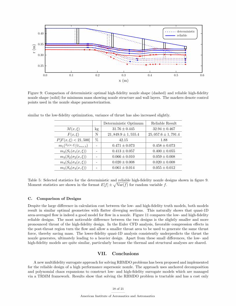
The reliable optimization terminated in an infeasible region after 3,599 unique function calls (including finitedifference) and 8 trust region iterations, however significant improvements in constraint feasibility weremade over the course of the optimization. In contrast, the deterministic optimization converged after 3,277unique function function calls. Both optimizations terminated with an active thrust constraint. Figure 9compares the reliable minimum mass nozzle geometry with the optimal deterministic minimum mass nozzlegeometry. Note the much larger throat radius in the reliable design to maintain adequate mass flow forthrust production as well as the less gradual and more pronounced throat shape leading to more reliablegeneration of supersonic flow in the divergent portion of the nozzle. Thin wall layers, minimum nozzle length,and careful baffle placement lead to lower mass for both designs.

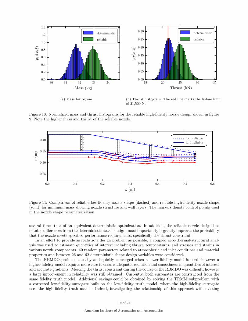
Table 5 compares selected statistics for the objective function mass M(x, ξ), the thrust F (x, ξ) whichwas the most critical constraint, and other constraints in the reduced RBMDO formulation. The other 5+temperature and stress constraints only differ by a few percent for each design and are not shown here. Figure10 compares the histograms of mass and thrust for each nozzle design. Statistics were calculated using 1million Monte Carlo samples on a polynomial chaos expansion calculated using level 1 sparse grid with theexception of mass, whose statistics were calculated using 10,000 Monte Carlo samples. The reliable designgenerates thrust much more reliably than the deterministic design for a small increase in mass, although

17 of 21


0.0 0.1 0.2 0.3 0.4 0.5 0.6

x (m)

0.25

0.30

0.35

0.40r

(m)

deterministicreliable

Figure 9: Comparison of deterministic optimal high-fidelity nozzle shape (dashed) and reliable high-fidelitynozzle shape (solid) for minimum mass showing nozzle structure and wall layers. The markers denote controlpoints used in the nozzle shape parameterization.

similar to the low-fidelity optimization, variance of thrust has also increased slightly.

Deterministic Optimum Reliable Result

M(x, ξ) kg 31.76± 0.445 32.94± 0.467

F (x, ξ) N 21, 849.9± 1, 555.4 25, 057.6± 1, 791.4

P [F (x, ξ) < 21, 500] % 42.15 1.88

m1(T2(x, ξ)/Tmax,2) - 0.471± 0.073 0.458± 0.073

m2(S1(σ1(x, ξ)) - 0.413± 0.057 0.400± 0.055

m3(S2(σ2(x, ξ)) - 0.066± 0.010 0.059± 0.008

m4(S3(σ3(x, ξ)) - 0.020± 0.008 0.020± 0.008

m5(S4(σ4(x, ξ)) - 0.061± 0.014 0.055± 0.012

Table 5: Selected statistics for the deterministic and reliable high-fidelity nozzle designs shown in figure 9.Moment statistics are shown in the format E[f ]±

√Var(f) for random variable f .

C. Comparison of Designs

Despite the large difference in calculation cost between the low- and high-fidelity truth models, both modelsresult in similar optimal geometries with flatter diverging sections. This naturally shows that quasi-1Darea-averaged flow is indeed a good model for flow in a nozzle. Figure 11 compares the low- and high-fidelityreliable designs. The most noticeable difference between the two designs is the slightly smaller and morepronounced throat of the high-fidelity design. In the Euler CFD analysis, favorable compression effects inthe post-throat region turn the flow and allow a smaller throat area to be used to generate the same thrustforce, thereby saving mass. The lower-fidelity quasi-1D analysis consistently underpredicts the thrust thenozzle generates, ultimately leading to a heavier design. Apart from these small differences, the low- andhigh-fidelity models are quite similar, particularly because the thermal and structural analyses are shared.

VII. Conclusions

A new multifidelity surrogate approach for solving RBMDO problems has been proposed and implementedfor the reliable design of a high performance supersonic nozzle. The approach uses anchored decompositionand polynomial chaos expansions to construct low- and high-fidelity surrogate models which are managedvia a TRMM framework. Results show that solving the RBMDO problem is tractable and has a cost only

18 of 21


30 31 32 33 34Mass (kg)

0.0

0.2

0.4

0.6

0.8

1.0

1.2

1.4

pM

(x,ξ

)deterministic

reliable

(a) Mass histogram.

15 20 25 30 35Thrust (kN)

0.00

0.05

0.10

0.15

0.20

0.25

0.30

pF(x,ξ

)

deterministic

reliable

(b) Thrust histogram. The red line marks the failure limitof 21,500 N.

Figure 10: Normalized mass and thrust histograms for the reliable high-fidelity nozzle design shown in figure9. Note the higher mass and thrust of the reliable nozzle.

0.0 0.1 0.2 0.3 0.4 0.5 0.6

x (m)

0.25

0.30

0.35

0.40

r (m

)

lo-fi reliablehi-fi reliable

Figure 11: Comparison of reliable low-fidelity nozzle shape (dashed) and reliable high-fidelity nozzle shape(solid) for minimum mass showing nozzle structure and wall layers. The markers denote control points usedin the nozzle shape parameterization.

several times that of an equivalent deterministic optimization. In addition, the reliable nozzle design hasnotable differences from the deterministic nozzle design; most importantly it greatly improves the probabilitythat the nozzle meets specified performance requirements, specifically the thrust constraint.

In an effort to provide as realistic a design problem as possible, a coupled aero-thermal-structural anal-ysis was used to estimate quantities of interest including thrust, temperatures, and stresses and strains invarious nozzle components. 40 random parameters related to atmospheric and inlet conditions and materialproperties and between 26 and 62 deterministic shape design variables were considered.

The RBMDO problem is easily and quickly converged when a lower-fidelity model is used, however ahigher-fidelity model requires more care to ensure adequate resolution and smoothness in quantities of interestand accurate gradients. Meeting the thrust constraint during the course of the RBMDO was difficult, howevera large improvement in reliability was still obtained. Currently, both surrogates are constructed from thesame fidelity truth model. Additional savings could be obtained by solving the TRMM subproblem witha corrected low-fidelity surrogate built on the low-fidelity truth model, where the high-fidelity surrogateuses the high-fidelity truth model. Indeed, investigating the relationship of this approach with existing

19 of 21


multifidelity, multi-level optimization approaches will be a subject of future research.The proposed approach also has several limitations. Although a reliable optimization is performed, the

specified reliability is actually quite low (99%). Estimating tail probabilities in chance constraints is a subjectof much research and even simply sampling the polynomial chaos expansion to accurately obtain a probabilitylevel of 10−7 can be prohibitively expensive. Importance sampling, reliability-index based methods, andapproaches like Conditional Value at Risk (CVaR) may prove useful for more efficiently estimating taildistributions. Another limitation is the original problem is not solved but rather approximated and replacedwith a high-fidelity surrogate based on a polynomial chaos expansion. Using higher sparse grid levels canmore accurately represent stochastic quantities of interest but only if the coefficients in the polynomial chaosexpansion converge rapidly.

Finally, we plan on further investigating the use of separable approaches for function approximation inuncertainty quantification, and carrying out a comparison of traditional RBDO methods with the methodproposed here.

Acknowledgments

This work was supported by the DARPA Enabling Quantification of Uncertainty in Physical Systemsprogram. R. Fenrich would additionally like to acknowledge the support of P. Avery and V. Menier for theirimportant contributions to the computational model development.

References

1Deaton, J. D., Design of Thermal Structures using Topology Optimization, Ph.D. thesis, Wright State University, 2014.2Martins, J. R. R. A. and Lambe, A. B., “Multidisciplinary Design Optimization: A Survey of Architectures,” AIAA

Journal , Vol. 51, No. 9, Sept. 2013, pp. 2049–2075.3Ahn, J. and Kwon, J. H., “An Efficient Strategy for Reliability-based Multidisciplinary Design Optimization using

BLISS,” Structural and Multidisciplinary Optimization, Vol. 31, No. 5, May 2006, pp. 363–372.4Tracey, B., Wolpert, D., and Alonso, J. J., “Using Supervised Learning to Improve Monte Carlo Integral Estimation,”

arXiv preprint arXiv:1108.4879 , 2011.5Madsen, H., Krenk, S., and Lind, N., Methods of Structural Safety, Prentice-Hall International Series in Civil Engineering

and Engineering Mechanics, Prentice-Hall, Inc., Englewood Cliffs, NJ, 1986.6Agarwal, H., Renaud, J., Lee, J., and Watson, L., “A Unilevel Method for Reliability Based Design Optimization,” AIAA,

April 2004.7Kleijnen, J. P., Ridder, A. A., and Rubinstein, R. Y., Variance Reduction Techniques in Monte Carlo Methods, Springer,

2013.8Geraci, G., Eldred, M., and Iaccarino, G., “A Multifidelity Control Variate Approach for the Multilevel Monte Carlo

Technique,” Center for Turbulence Research Annual Research Briefs, 2015.9Liao, Q. and Zhang, D., “Probabilistic Collocation Method for Strongly Nonlinear Problems: 1. Transform by Location:

Transformed Probabilistic Collocation Method,” Water Resources Research, Vol. 49, No. 12, Dec. 2013, pp. 7911–7928.10Xiu, D. and Karniadakis, G. E., “Modeling Uncertainty in Flow Simulations via Generalized Polynomial Chaos,” Journal

of Computational Physics, Vol. 187, No. 1, May 2003, pp. 137–167.11Lukaczyk, T. W., Surrogate Modeling and Active Subspaces for Efficient Optimization of Supersonic Aircraft , Ph.D.

thesis, Stanford University, June 2015.12Goda, T., “On the Separability of Multivariate Functions,” arXiv preprint arXiv:1301.5962 , 2013.13Constantine, P. G., Active Subspaces: Emerging Ideas for Dimension Reduction in Parameter Studies, No. 2 in SIAM

Spotlights, Society for Industrial and Applied Mathematics, Philadelphia, 2015.14Rodriguez, J. F., Renaud, J. E., Wujek, B. A., and Tappeta, R. V., “Trust Region Model Management in Multidisciplinary

Design Optimization,” Journal of Computational and Applied Mathematics, Vol. 124, No. 1, 2000, pp. 139–154.15Eldred, M. S. and Dunlavy, D. M., “Formulations for Surrogate-Based Optimization with Data Fit, Multifidelity, and

Reduced-order Models,” Proceedings of the 11th AIAA/ISSMO Multidisciplinary Analysis and Optimization Conference,AIAA-2006-7117, Portsmouth, VA, Vol. 199, 2006.

16Eggers, J. M., “Supersonic Axisymmetric Jet Flow,” 1966.17Prautzsch, H., Boehm, W., and Paluszny, M., Bezier and B-Spline Techniques, Mathematics and Visualization, Springer

Berlin Heidelberg, Berlin, Heidelberg, 2002.18Holmberg, E., Torstenfelt, B., and Klarbring, A., “Stress Constrained Topology Optimization,” Structural and Multidis-

ciplinary Optimization, Vol. 48, No. 1, July 2013, pp. 33–47.19Martins, J. and Poon, N. M., “On Structural Optimization using Constraint Aggregation,” VI World Congress on

Structural and Multidisciplinary Optimization, Rio de Janeiro, Brazil , 2005.20Tu, J., Choi, K. K., and Park, Y. H., “A New Study on Reliability-Based Design Optimization,” ASME Journal of

Mechanical Design, Vol. 121, No. 4, 1999, pp. 557–564.21Jursa, A. S., Handbook of Geophysics and the Space Environment , Air Force Geophysics Laboratory, 4th ed., 1985.

20 of 21


22“Pratt & Whitney F100,” IHS Jane’s Defense and Security Intelligence and Analysis, 2017.23Lee, A. S., Singh, R., and Probert, S. D., “Modeling of the Performance of a F100-PW229 Equivalent Engine under

Sea-Level Static Conditions,” 45th AIAA/ASME/SAE/ASEE Joint Propulsion Conference and Exhibit , 2009.24Camm, F., “The Development of the F100-PW-220 and F110-GE-100 Engines: A Case Study of Risk Assessment and

Risk Management,” 1993.25Bansal, N. P., Handbook of Ceramic Composites, Kluwer Academic Publishers, 2005.26Chawla, K. K., Ceramic Matrix Composites, Springer US, Boston, MA, 2003.27Cytec, “CYCOM 5250-4 Prepreg System,” March 2012, AECM-00008 datasheet.28Hexcel, “HexTow IM7,” 2016, CTA351 JY16 datasheet.29Benecor, I., “Engineering Honeycomb Structures,” 2016, Datasheet.30Eldred, M. S., Giunta, A. A., Collis, S. S., Alexandrov, N. A., Lewis, R. M., and others, “Second-order Corrections for

Surrogate-based Optimization with Model Hierarchies,” Proceedings of the 10th AIAA/ISSMO Multidisciplinary Analysis andOptimization Conference, Albany, NY, Aug, 2004, pp. 2013–2014.

31Ghanem, R. G. and Spanos, P. D., Stochastic Finite Elements: A Spectral Approach, Springer, New York, NY, 1991.32Eldred, M., Webster, C., and Constantine, P., “Evaluation of Non-Intrusive Approaches for Wiener-Askey Generalized

Polynomial Chaos,” American Institute of Aeronautics and Astronautics, April 2008.33Xiu, D. and Hesthaven, J. S., “High-Order Collocation Methods for Differential Equations with Random Inputs,” SIAM

Journal on Scientific Computing, Vol. 27, No. 3, Jan. 2005, pp. 1118–1139.34Adams, B. M., Ebeida, M. S., Eldred, M. S., Jakeman, J. D., Swiler, L. P., Stephens, J. A., Vigil, D. M., Wildey, T. M.,

Bohnhoff, W. J., Dalbey, K. R., Eddy, John P., Hooper, Russell W., Hu, Kenneth T., Bauman, Lara E., Hough, Patricia D., andRushdi, Ahmad, “Dakota, A Multilevel Parallel Object-Oriented Framework for Design Optimization, Parameter Estimation,Uncertainty Quantification, and Sensitivity Analysis: Version 6.3 User’s Manual,” Tech. Rep. SAND2014-4633, Sandia NationalLaboratories, July 2014.

35Geuzaine, C. and Remacle, J.-F., “Gmsh: A 3-D Finite Element Mesh Generator with Built-in Pre-and Post-processingFacilities,” International Journal for Numerical Methods in Engineering, Vol. 79, No. 11, 2009, pp. 1309–1331.

36Sanchez, R., Palacios, R., Economon, T. D., Kline, H. L., Alonso, J. J., and Palacios, F., “Towards a Fluid-StructureInteraction Solver for Problems with Large Deformations Within the Open-Source SU2 Suite,” American Institute of Aeronauticsand Astronautics, Jan. 2016.

37Menier, V., Numerical Methods and Mesh Adaptation for Reliable RANS Simulations, Ph.D. thesis, Paris 6, 2015.38Farhat, C., “AERO-S,” https://bitbucket.org/frg/aero-s/overview, 2017.39Philip, E., Murray, W., and Saunders, M. A., “Users Guide for SNOPT Version 6, a Fortran Package for Large-scale

Nonlinear Programming,” University of California, California, 2002.

21 of 21


Documents

Reliable Multidisciplinary Design of a Supersonic …adl.stanford.edu/papers/fenrich-2017.pdfReliable Multidisciplinary Design of a Supersonic ... approach can be used to e ectively