Reliable p-median facility location problem: two-stage robust

models and algorithms

Yu An, Bo Zeng, Yu Zhang and Long Zhao

Dept. of Industrial and Management Systems Engineering

Dept. of Civil and Environment Engineering

University of South Florida, Tampa, FL 33620

December, 2012

Abstract

In this paper, we propose a set of two-stage robust optimization models to design reliable

p-median facility location networks subject to disruptions. A customized column-and-constraint

generation approach is implemented and shown to be more effective than Benders cutting plane

method. Numerical experiments are performed on real data and management insights on system

design are presented. Our study also demonstrates the strong modeling capability of two-stage

robust optimization scheme by including two practical issues, i.e., facility capacities and demand

losses due to disruptions, which receive little attention in reliable network design research.

Results show the significant influence of the demand loss factor on the network configuration.

keyword: facility location problem, reliable network design, two-stage robust optimization, de-

mand loss

1 Introduction

The selection of facility locations and customer assignments are among the most crucial issues in

designing an efficient distribution network. To address these issues, various facility location models

are formulated and studied for decades, including those based on p-median and fixed-charge facility

location formulations and their extensions (Daskin, 1995; Drezner, 1995; Revelle et al., 2008; Melo

et al., 2009). The applications of those facility location models can be found in various industries,

including manufacturing, retail and healthcare (Barahona and Jensen, 1998; Teo and Shu, 2004;

Jia et al., 2007). Although it is expected by designers that the distribution network works reliably,

network components could lose their functions and become unavailable in practice. For example,

some facilities may be disrupted by natural disasters, labor strikes or terrorism threats, and become

non-operable. Since the material or information flows are generated, processed, and distributed by

facilities, facility disruptions could significantly deteriorate the performance of the whole network

and result in enormous economic losses, see the descriptions in Snyder et al. (2010) and references

therein.

To address this reliability issue, several recent studies, including Snyder and Daskin (2005),

Berman et al. (2007), Cui et al. (2010), Li and Ouyang (2010), Lim et al. (2010), Li et al. (2012),

and Peng et al. (2011) propose to proactively consider network disruptions and the incurred cost

of countermeasures in the system design stage. The countermeasures, i.e., mitigation or recourse

operations, are to reassign clients to survived facilities such that they can be served and the impact

1

of disruptions can be minimized. Hence, the objective of system design is to minimize the (weighted)

overall cost, including the operation cost in the normal situation when all facilities function properly,

and the cost of mitigation in disruptive situations. To analytically represent this new design scheme,

based on the explicit probabilistic information, several compact (nonlinear) mixed integer programs

or scenario-based two-stage stochastic programming formulations are developed and customized

exact or approximation algorithms are designed to solve real instances. (Snyder and Daskin, 2005;

Cui et al., 2010; Li and Ouyang, 2010; Lim et al., 2010; Shen et al., 2011; Peng et al., 2011).

Nevertheless, in many situations, either accurate method does not exist or sufficient data are

lack to exactly characterize probability distributions, or data are contaminated to provide precise

information. Under such situations, probabilistic models, e.g., the aforementioned two types of

models, could be inappropriate or lead to infeasible solutions. To address this challenge, robust

optimization (RO) method, which simply assumes an uncertainty set to capture random data, is

developed to provide solutions that are robust to any perturbations within the uncertainty set. To

model the situation where some decisions can be made and implemented after the uncertainty is

revealed, robust optimization is extended to include the second stage recourse decisions so that

the available information can be fully utilized to produce a less conservative solution. After their

introduction, original robust optimization method and its two-stage extension have been applied

in many operational and engineering areas (Ben-Tal et al., 2009; Bertsimas et al., 2011), such as

facility location problems with random demands (Atamturk and Zhang, 2007; Baron et al., 2011;

Gabrel et al., 2011). In fact, comparing with demand uncertainty, facility disruptions are often

less likely to be described by accurate probabilistic information. For example, earthquakes in

California or hurricanes in Florida could cause facilities in those regions to be disrupted. However,

it is very difficult to estimate the number of earthquakes or hurricanes in next 10 years based

on historical/statistical data. Hence, in this paper, we apply the concept of uncertainty set to

capture the possible site disruptions and employ robust optimization method to study reliable

facility location problems.

Specifically, we adopt two-stage robust optimization approach to investigate reliable p-median

problem, where location decisions are made before (here-and-now) and recourse (mitigation) de-

cisions are made after disruptions are revealed (wait-and-see). We mention that such a modeling

framework exactly captures the decision making sequence in real operations. In particular, due to

its strong modeling capability, we are able to extend our study to consider facility capacities and

demand losses due to disruptions. We note that the former situation is very challenging for proba-

bilistic models while the latter has not been investigated in existing literature. Then, classical and

customized solution algorithms, i.e., Benders decomposition and column-and-constraint generation

methods, are implemented and a set of numerical experiments are performed to generate insights

on the algorithm performance and the network design.

The rest of the paper is organized as follows. In Section 2, we review relevant literature on

probabilistic models and two-stage robust optimization models. In Section 3, we introduce our

two-stage robust optimization reliable p-median models and analyze their properties. In Section

4 we describe our solution algorithms. In Section 5, we present numerical results and provide

insights on system design. In Section 6, we conclude this paper with a discussion on future research

directions.

2

2 Literature review

In this section, we briefly review two types of relevant studies on the facility location problem:

probability based reliable facility location models and (two-stage) robust optimization ones. Results

on classical and deterministic facility location problems can be found in Daskin (1995) and Drezner

(1995). For problems with uncertain demands and cost, readers are referred to a comprehensive

review in Snyder (2006).

The research by Drezner (1987) is probably the first one studying facility location problem with

unreliable facilities while Snyder and Daskin (2005) present the first reliable facility location mod-

els with inclusion of mitigation/recourse operations and costs. Lagrangian relaxation algorithms

are implemented within a branch-and-bound scheme to solve the resulting linear mixed integer

programs for real instances. By relaxing the assumption that all sites share the same failure rate,

Cui et al. (2010) build a nonlinear mixed integer program and develop both Lagrangian relaxation

and continuum approximation algorithms for this challenging problem. To reduce the complexity

of the nonlinear form, Lim et al. (2010) study a simplified model where clients will be assigned

to (unreliable) facilities and reliable backup facilities if needed. Shen et al. (2011) present both

scenario-based stochastic programming and a nonlinear mixed integer programming model and

show that they are generally equivalent. Also, a constant-ratio approximation algorithm for the

case where all failure rates are identical is proposed. Li and Ouyang (2010) study a problem with

correlated probabilistic disruptions and solve their model by a continuum approximation algorithm.

Li et al. (2012) consider problems with a fortification budget in the first stage so that unreliable

facilities can be fortified by hardening operations. Recently, this line of research is extended to

investigate more general reliable network design problems. Peng et al. (2011) consider a reliable

multiple-echelon logistics network design problem where disruptions can happen in multiple eche-

lons. An et al. (2011) study reliable hub-and-spoke network design problems in which hubs could

be disrupted and affected flows will be rerouted through survived operational hubs. From those

aforementioned studies, we observe that (i) either complicated nonlinear mixed integer programs or

large-scale scenario-based stochastic programs are necessary to build the model. When professional

solvers are not efficient to deal with those models, customerized algorithms, either analytical or

heuristic ones, will be developed; (ii) some practical situations are not sufficiently investigated. For

example, very limited research is done for capacitated models except Peng et al. (2011) and no

exact algorithm has been developed. Also, demand losses due to disrupted clients have not been

modeled, which could affect the location of facilities.

Different from nonlinear mixed integer programs or scenario-based stochastic programs that are

developed based on precise probabilistic information, robust optimization based location models,

including those developed with two-stage robust optimization method, assume a probability-free

uncertainty set and seek to determine locations that are robust to any perturbations in that uncer-

tainty set. Baron et al. (2011) build a multi-period capacitated fixed charge (single-stage) robust lo-

cation model and investigate the impact of different uncertainty sets on facility locations. Gulpınar

et al. (2012) propose to use tractable (single-stage) robust optimization method to approximately

solve stochastic facility location problem with a chance constraint. Atamturk and Zhang (2007),

Gabrel et al. (2011), and Zeng and Zhao (2011) develop two-stage robust optimization formulations

for location-transportation problems where locations and capacities must be determined in the first

stage and transportation decisions can be adjusted after demand is realized. Different solution al-

gorithms are proposed by them respectively, including an approximation algorithm (Atamturk and

Zhang, 2007), Benders cutting plane algorithm (Gabrel et al., 2011), and the column-and-constraint

3

generation (C&CG) algorithm (Zeng and Zhao, 2011). We mention that the column-and-constraint

generation algorithm demonstrates a superior computational performance over Benders cutting

plane method in the two-stage facility location problem and power system scheduling problems

(Zhao and Zeng, 2010).

In order to make this paper focused, we restrict this study to p-median problem and leave

the study of two-stage RO formulations for another classical model, i.e., the fixed-charge facility

location problem, as a future research direction. Research presented in this paper makes the

following contributions to the literature.

(i) To the best of our knowledge, no research has been done to apply two-stage RO to formulate

reliable facility location design problems with consideration of disruptions. Hence, this paper

presents the first set of reliable facility location formulations using two-stage robust optimization

tools.

(ii) Because of the modeling advantages of two-stage RO, we consider real features that have

received very limited or no attention. They are finite capacities of facilities and demand losses due

to disruptions.

(iii) In addition to some analytical study on those models, we customize and implement solution

algorithms to perform numerical experiments. We also present management insights based on the

numerical results from instances with real data.

3 Two-stage robust p-median reliable models

In this section, we present our formulations on two-stage RO reliable p-median facility location

problem. We first consider uncapacitated robust models and then extend our work to consider

capacitated cases. Existing research generally ignores the demand losses due to disruptions. We

show that, by using the two-stage robust optimization framework, demand losses can be easily

incorporated. We also derive structural properties of those models.

3.1 Robust p-median models without demand losses

Different from stochastic programming models that explicitly consider all possible uncertain sce-

narios, (two-stage) robust optimization models use an uncertainty set to describe the concerned

possible scenarios without depending on probability information. Specifically, assume that all sites

in set J are homogeneous and consider all possible scenarios with up to k simultaneous disruptions.

Then, the uncertainty set, i.e., the disruption set in this paper, can be represented as

A = {z ∈ {0, 1}|J | :∑j∈J

zj ≤ k}. (1)

where zj is the indicator variable for site j, i.e., zj = 1 if site j is disrupted and zj = 0 otherwise.

Note that, although there may exist an exponential number of disruptive scenarios, this formulation

provides an implicit but compact algebraic format to capture all of them. In the remainder of this

paper, unless explicitly mentioned, we employ this disruption set to perform our study.

Next, we develop our two-stage RO reliable p-median facility location models. Let I be the

set of clients (customer nodes) and J ⊆ I be the set of potential facility nodes. Without loss of

generality, we assume that I = J . Each client i ∈ I has a demand di and the unit cost of serving

i by the facility at j ∈ J is cij ≥ 0 with cii = 0. We use y and x to denote the first stage (the

normal situation without disruptions) decision variables: yj = 1 means that a facility is located

4

at j, yj = 0 otherwise; xij ∈ [0, 1] represents the portion of i’s demand served by j in the normal

situation. Note that the first stage decision variables are to be fixed before any disruptive scenario

z in set A is realized. In a disruptive scenario, as in Snyder and Daskin (2005) and Cui et al. (2010),

a disrupted facility at j can not serve any client. However, system reliability can be achieved by

implementing recourse or mitigation operations such as re-assigning customers to survived facilities.

So, we introduce w and q to represent the second stage recourse operation decisions in a disruptive

scenario, where wij ∈ [0, 1] represents the portion of demand di served by the survived facility at j

and qi ∈ [0, 1] represents the unsatisfied portion. Each unit of unsatisfied demand of di will incur

a penalty M .

Similar to all existing studies on reliable facility location models, we first assume that there is

no demand loss in any disruptive scenario, i.e., disruptions only affect the function of facilities and

all clients keep generating demands as usual. In the following, we present the two-stage RO reliable

p-median facility location formulation with up to k simultaneous disruptions and no demand loss.

RO-PMP0

V0(p, k, ρ) =minx,y

(1− ρ)∑i

∑j

cijdixij + ρmaxz∈A

min(w,q)∈S0(y,z)

(∑i

∑j

cijdiwij +∑i

Mdiqi) (2)

s.t. xij ≤ yj , ∀i, j (3)∑j

xij ≥ 1, ∀i (4)

∑j

yj = p, (5)

xij ≥ 0, ∀i, j; yj ∈ {0, 1}, ∀j (6)

where

S0(y, z) = {wij ≤ 1− zj , ∀i, j (7)

wij ≤ yj , ∀i, j (8)∑j

wij + qi ≥ 1, ∀i (9)

wij ≥ 0, ∀i, j; qi ≥ 0, ∀i } (10)

In this formulation, the objective function in (2) seeks to minimize the weighted sum of the

operation costs in the normal disruption-free situation and in the worst disruptive scenarios in

A. The weight ρ ∈ [0, 1] is a parameter that reflects the system designer’s attitude towards the

disruption cost. Clearly, a larger ρ indicates that the designer is more conservative and willing

to configure the system in a way such that less recourse/mitigation operation costs will incur in

disruptive situations. Constraints in (3)-(5) are from the classical p-median model and simply mean

that a customer site can be assigned to a facility only if the facility is built, the entire demand of

a customer site has to be served, and the total number of facilities is p, respectively.

The max operator identifies the disruptive scenario(s) in A yielding the largest operation cost,

given the location y. The second min seeks for the least costly mitigation solution while the

set S0(y, z) defines the possible recourse operations. That is, given the definition of yj and zj ,

constraints (7) and (8) ensure that in any disruptive scenario, a client i’s demand can only be

assigned to established and survived facilities. Then, constraints in (9) represents that except the

lost portion qi, the rest of i’s demand, 1− qi, has to be served. In this paper, our research focuses

on the nontrivial cases where k ≤ p − 1. Otherwise, there will be no mitigation operations in any

5

worst disruption scenario and the problem reduces to the p-median formulation.

Although this robust formulation is a complicated tri-level optimization problem, we can derive

some structural properties by analyzing the underlying location problem. Specifically, we consider

the case where the penalty coefficient M is sufficiently large, e.g., M ≥ maxi,j{cij}. It implies that

all customer demands will be served in any disruptive situation because the penalty cost is higher

than the largest serving cost. Actually, every individual customer’s demand will be served by an

available facility that is closest to him, in both normal and disruptive situations. Clearly, given

that some customer’s initially assigned facility becomes unavailable in a disruptive situation, his

demand will be served by a survived facility that is definitely further. Hence, we have the following

result.

Lemma 1. For given a facility location y0, let Cr(y0) and Cz(y0) be the operating costs in the

normal situation and a disruptive situation z, respectively. When M is sufficiently large, we have

Cz(y0) ≥ Cr(y0).

Consequently, the following results can be proven easily.

Proposition 1. When M is sufficiently large, the function V0(p, k, ρ) is (i) non-increasing with

respect to p; (ii)non-decreasing with respect to k; and (iii) non-decreasing with respect to ρ;

Proof. Statements in (i) and (ii) are very easy to prove. We give the proof for the statement in

(iii). Consider ρ1 ≤ ρ2 and their corresponding optimal facility locations y1 and y2.

Clearly, as y2 may not be optimal when ρ = ρ1, we have

V0(p, k, ρ1) = V0(p, k, ρ1|y = y1) ≤ V0(p, k, ρ1|y = y2).

Given that ρ1 ≤ ρ2, it follows from Lemma 1 that

V0(p, k, ρ1|y = y2) ≤ V0(p, k, ρ2|y = y2).

Therefore, we have

V0(p, k, ρ1) = V0(p, k, ρ1|y = y1) ≤ V0(p, k, ρ2|y = y2) = V0(p, k, ρ2)

Note from constraints (3)-(10) that the two-stage RO is a very adaptive modeling framework. By

using y and z, we can impose logic or physical restrictions on recourse decisions without enumerating

all their possible values. In the following, we show that a more involved situation can be formulated

compactly.

3.2 Robust p-median problem with demand losses

Note that the aforementioned formulation assumes that a disrupted site keeps generating demands

as usual while a facility on it, if exists, loses the function. However, as an example, demands of

non-essential or luxury products often vanish in disruptions. To the best of our knowledge, no

existing work on the reliable facility location problem studies the impact of demand losses due

to site disruptions on the system design. One possible reason is that, if the demand loss factor

is considered, classical probabilistic models have to evaluate all possible scenarios while different

scenarios will have different coefficients in their objective functions, which makes it very challenging

6

to have a compact and tractable formulation. Nevertheless, the two-stage robust optimization

scheme provides us a convenient modeling framework to address this issue. Specifically, given the

interpretation of zi in (1), we can simply add “−zi” on the right-hand-side of (9) to model the

demand loss at a disrupted site.

RO-PMPl

Vl(p, k, ρ) =minx,y

(1− ρ)∑i

∑j

cijdixij + ρmaxz∈A

min(w,q)∈Sl(y,z)

(∑i

∑j

cijdiwij +∑i

Mdiqi)

(11)

s.t. (3)− (6),

with

Sl(y, z) = {(7)− (8), (10)∑j

wij + qi ≥ 1− zi, ∀i} (12)

Note from (12) that when zi = 1, the minimization recourse problem will drive wij = 0 for all j

and qi = 0, i.e., there is no demand at i to serve.

We mention that considering demand losses complicates the problem structure as the customer

demand in a disruptive situation is depending on z now. Nevertheless, we note that in RO-PMPl,

if M is sufficiently large, the operation cost of the worst disruptive situation is still larger than that

of the normal situation.

Lemma 2. When M is sufficiently large, consider a given facility location y∗ and the disruption

set A. We have (i) the worst case disruptions and therefore demand losses happen only at facility

sites, i.e., those with y∗j = 1; (ii) CA(y∗) ≥ Cr(y

∗) where CA(y∗) is the operating cost of the worst

case scenario in A.

Proof. For (i), we prove it by contradiction. Consider the worst case disruptive situation z1 where

a disruption happens at site j0, on which there is no facility, i.e., z1j0 = 1 and y∗j0 = 0. Let C1 be

the operation cost under this disruptive situation.

As p− k ≥ 1, there exists a facility, say j1 with y∗j1 = 1, survived in the disruptive situation z1.

Consider two disruptive situations: z′ where z′j0 = 0, and z′j = z1j for j = j0, and z2 where z2j0 = 0,

z2j1 = 1 and z2j = z1j for j = j0 and j = j1. Denote the operation cost under z′ by C ′, and that

under z2 by C2.

First, it is clear that C ′ ≥ C1, because demand from customer site j0 must be served by some

facility in z′ while this demand is lost in z1 and does not incur any cost.

Second, under the disruptive situation z2, because the facility at j1 is not available, all its served

customer demands, except the demand from j1, will be served by other survived facilities, which

will be further and more costly. Because cj1j1 = 0, the demand from site j1 will not incur any

service cost in z′ and z2. So, we have C2 ≥ C ′.

Because C2 ≥ C ′ ≥ C1, we have the desired contradiction. Also, based on the argument

of C ′ ≤ C2, it is easy to see that CA(y∗) is non-decreasing with respect to k and therefore (ii)

follows.

As a result, similar to those presented in Proposition 1, the following properties for RO-PMPl

can be obtained based on Lemma 2.

7

Proposition 2. When M is sufficiently large, the function Vl(p, k, ρ) is (i) non-increasing with

respect to p; (ii) non-decreasing with respect to k; and (iii) non-decreasing with respect to ρ.

Next, we extend our study to capacitated facility location problem, whose reliable models have

received little research attention.

3.3 The robust capacitated facility location model

The capacitated p-median facility location (CPMP) problem is an extension of the classical facility

location model. Besides the same objective function and decision variables as in the classical

uncapacitated facility location problem, it assumes that each potential facility has a capacity, i.e.,

an upper bound on the amount of demand that it can serve (Sridharan, 1995). Let Cj denote the

capacity of site j. The two-stage robust capacitated p-median facility location problem without

demand loss is shown as follows:

RO-CPMP0

VC0(p, k, ρ) =minx,y

(1− ρ)∑i

∑j

cijdixij + ρmaxz∈A

min(w,q)∈S0(y,z)

(∑i

∑j

cijdiwij +∑i

Mdiqi) (13)

s.t. (3)− (6)∑i

dixij ≤ Cjyj , ∀j (14)

with

S0(y, z) = {(7)− (9), (10)∑i

diwij ≤ Cjyj , ∀j} (15)

Constraints (14) ensure that the total demand served by facility j does not exceed its capacity Cj .

Constraints (15) impose the similar requirement on the survived facility j.

Consider a disruptive situation, when M is sufficiently large, demands will either be completely

served; or if the remaining capacity is not sufficient, some of them will be lost and penalized with

M per unit. So, we can derive some insights on RO-CPMP0, although it has a more complicated

structure. Specifically, for a given facility location y0 and a disruptive situation z, since x, w, and

q are continuous, we need to solve two linear programs to determine the operation costs Cr(y0)

and Cz(y0). It is easy to see that an optimal solution of the recourse problem of the disruptive

situation is either a feasible solution to the first-stage problem or can be converted into a feasible

solution by assigning the lost demand to facilities.

Lemma 3. When M is sufficiently large, for a given facility solution y0 and a disruptive situation

z, if there is no demand loss due to disruptions, we have Cz(y0) ≥ Cr(y0).

Similarly, we have the following properties on VC0(p, k, ρ).

Proposition 3. When M is sufficiently large, the function VC0(p, k, ρ) is (i) non-increasing with

respect to p; (ii)non-decreasing with respect to k; and (iii) non-decreasing with respect to ρ;

We can also extend our study with a little modification to model demand losses if a disrupted

site does not generate demand. The formulation is

8

RO-CPMPl

VCl(p, k, ρ) =minx,y

(1− ρ)∑i

∑j

cijdixij + ρmaxz∈A

min(w,q)∈Sl(y,z)

(∑i

∑j

cijdiwij +∑i

Mdiqi) (16)

s.t. (3)− (6), (14)

with

Sl(y, z) = {(7), (8), (10), (12), (15)}

Because of the demand losses and facility capacity constraints, RO-CPMPl is less trackable than

previously studied models. Nevertheless, under some mild assumptions, properties similar to those

models can be derived.

Specifically, we assume that (i) Cj ≥ dj for all j, and (ii) the service costs satisfy the triangular

inequality. The first assumption indicates that in both normal and disruptive situations, it is

feasible to serve the whole demand of a (survived) facility site by the facility itself. The second

assumption shows that it always leads to less cost to serve the demand of a (survived) facility site

by the facility on it. Finally, given that cjj = 0, it can be proven, by the same line of Lemma 2, that

a customer site disruption actually decreases the operation cost while the disruption of one facility

site will lead to more operation cost. Hence, we have the following property similar to Lemma 2.

Lemma 4. Under assumptions (i) and (ii), when M is sufficiently large, consider a given facility

solution y∗ and a disruption set A. We have that (i) the worst case disruptions and therefore

demand losses happen only at facility sites, i.e., those with y∗j = 1; (ii) CA(y∗) ≥ Cr(y

∗) where

CA(y∗) is the operating cost in the worst disruptive situation in A.

Finally, we have

Proposition 4. Under assumptions (i) and (ii), when M is sufficiently large, the function VCl(p, k, ρ)

is (i) non-increasing with respect to p; (ii) non-decreasing with respect to k; and (iii) non-decreasing

with respect to ρ.

4 Solution algorithms

Two-stage RO models in general are very difficult to solve (Ben-Tal et al., 2004). When the

second stage mitigation problem is a linear program (LP), as in each of the models we introduced

so far, Benders decomposition method can be employed to derive optimal solutions (Bertsimas

et al., 2012; Jiang et al., 2011). However, Benders method is not efficient in dealing with real size

instances. A different solution method, the column-and-constraint generation algorithm, denoted

by C&CG, was developed in Zeng and Zhao (2011) recently, which shows a superior performance

over Benders method in solving practical problems. In this paper, we adopt C&CG method as

the primary solution method to solve two-stage RO reliable p-median facility location models. We

first provide details of a customized C&CG method for our robust models and then present a set

of improvement strategies. We also briefly discuss the implementation of Benders decomposition

method. Our computational study also confirm the efficiency of C&CG algorithm over Benders

decomposition method.

9

4.1 Implementation of C&CG algorithm

We select RO-PMPl to describe the development of the customized C&CG algorithm. Because other

three robust models are of similar structures, C&CG can be implemented with minor modifications

to solve them.

C&CG algorithm is implemented within a two level master-sub problem framework. In the

subproblem, for a given solution (x∗,y∗) to the first stage decision problem, we solve the remaining

max-min problem to identify the worst scenario. As the unsatisfied demand will be penalized in

any disruptive situation, the second stage mitigation problem is always feasible. Hence, we can take

the dual and obtain a max-max problem, which is actually a maximization problem. Specifically,

let u, v, and s be the dual variables of the constraints (7), (8) and (12) respectively. The resulting

nonlinear maximization formula of subproblem is as follows:

NL-SP

maxz,u,v,s

∑i

∑j

(1− zj)uij +∑i

∑j

y∗j vij +∑i

(1− zi)si (17)

s.t. uij + vij + si ≤ cijdi, ∀i, j (18)

si ≤ Mdi, ∀i (19)∑j∈J

zj ≤ k, (20)

uij ≤ 0, ∀i, j; vij ≤ 0, ∀i, j; si ≥ 0, ∀i; zj ∈ {0, 1}, ∀j (21)

As the nonlinear terms are the products of a continuous variable and a binary variable, we can

linearize this formulation by replacing them with two new variables, i.e., Uij = uijzj and Si = sizi,

and using big-M method. Given the penalty coefficient M in (2), the big M for Uij and Si can be

set to Mdi. As a result, the linearized subproblem is:

SP

maxz,u,v,s,U,S

∑i

∑j

(uij − Uij + y∗j vij) +∑i

(si − Si) (22)

s.t. uij + vij + si ≤ cijdi, ∀i, j (23)

si ≤ Mdi, ∀i (24)

Uij ≥ uij , ∀i, j (25)

Uij ≥ −Mdizj , ∀i, j (26)

Uij ≤ uij +Mdi(1− zj), ∀i, j (27)

Si ≤ si, ∀i (28)

Si ≤ Mdizi, ∀i (29)

Si ≥ si +Mdi(zi − 1), ∀i (30)∑j∈J

zj ≤ k, (31)

uij ≤ 0, ∀i, j;Uij ≤ 0, ∀i, j; vij ≤ 0, ∀i, j;si ≥ 0, ∀i;Si ≥ 0, ∀i; zj ∈ {0, 1}, ∀j (32)

Note that the linearized subproblem (SP), which is a MIP problem, can be solved by a profes-

sional MIP solver. Next, we describe the details of the column-and-constraint generation algorithm

10

along with the formulation of the master problem, which will be solved iteratively. In each iteration

n, a significant scenario zn will be identified through solving the SP. Then, a set of recourse vari-

ables (wn,qn) and corresponding constraints in the forms of (34) and (35)-(37) associated with this

particular scenario will be created and added to the master problem. Let UB and LB be the upper

and lower bounds respectively, Gap be the relative gap between UB and LB, n be the iteration

index and ϵ be the optimality tolerance.

Column-and-constraint generation algorithm

1. Set LB = −∞, UB = ∞, and n = 0.

2. Solve the following master problem (MP) and obtain an optimal solution (xn,yn, ηn) (a

feasible solution if unbounded) and set LB to the optimal value of the MP.

MP

min (1− ρ)∑i

∑j

cijdixij + ρη (33)

s.t. (3)− (6)

η ≥∑i

∑j

cijdiwlij +

∑i

Mdiqli, ∀l = 1, 2, ..., n (34)

∑j

wlij ≥ 1− qli − zli, ∀i, l = 1, 2, ..., n (35)

wlij ≤ 1− zlj , ∀i, j, l = 1, 2, ..., n (36)

wlij ≤ yj , ∀i, j, l = 1, 2, ..., n (37)

qli ≥ 0, ∀i, l = 1, 2, ..., n;wlij ≥ 0, ∀i, j, l = 1, 2, ..., n. (38)

3. Solve SP with respect to (xn,yn) and derive an optimal solution (zn,un,vn, sn) and its

optimal value Rn. Update

UB = min{UB, (1− ρ)∑i

∑j

cijdixnij + ρRn}.

4. If Gap = UB−LBLB ≤ ϵ, an ϵ-optimal solution is found, and terminate. Otherwise, create

recourse variables (wn,qn) and corresponding constraints associated with zn and add them

to MP. Update n = n+ 1. Go to Step 2. �

It has been proven in Zeng and Zhao (2011) that C&CG algorithm converges to an optimal solution

in finite iterations. Different from C&CG method, after solving SP, Benders decomposition method

will iteratively supply a single cutting plane in the following form to its master problem that only

carries the first stage decision variables (x,y)

η ≥∑i

∑j

(1− znj )unij +

∑i

∑j

vnijyj +∑i

(1− zni )sni

Comparing these two types of algorithms, Zeng and Zhao (2011) theoretically show that C&CG

method is of a much less computational complexity and its generated constraints are stronger.

11

4.2 Algorithm improvement

In this section, we study how to improve the computational performance of C&CG method on

solving reliable p-median facility location problems. In particular, note that the numbers of variables

and constraints in MP will quickly increase over iterations. So, solving MP to optimality may take

excessive amount of time for large instances. To address this challenge, a few strategies could be

applied to reduce the computational expenses on solving MP.

Adding valid inequalities to MP. Two types of valid inequalities are generated. The first type

is generally applicable for any implementation of C&CG. That is, let t denote the objective value

of the current MP. Then, the following constraint

t ≥ LB (39)

is valid and can be added to MP to speed up the branch-and-bound procedure of the solver. The

second type is specific to our reliable facility location problems. Based on Proposition 1-4, it can

be seen that, when M is sufficiently large, t can be bounded from below by the optimal values of

instances with smaller k and ρ. Moreover, instances with smaller ρ and k are easier to compute.

Therefore, constraint similar to (39) can be added to MP once the optimal value of an instance

with smaller ρ or k is available.

Passing significant disruptive scenarios. Similarly, as instances with smaller ρ are easier to com-

pute, we can first solve such an instance (with a small ρ) to obtained a set of disruptive scenarios.

Those scenarios, i.e., the corresponding recourse variables and constraints, can be supplied to the

MP of an instance with a larger ρ. Intuitively speaking, those scenarios, which yield the most

disruptive cost, should also be significant even when ρ is larger. Hence, C&CG algorithm can avoid

starting an MP from scratch, less iterations in C&CG can be expected. Nevertheless, we note that

it also has a negative effect as MP will be larger and its computational time could be longer.

Obtaining good solutions before convergence. Note that MP gradually evolves into a large and

computationally intensive mixed integer program while any of its feasible solutions can be used to

generate valid disruptive scenarios. So, when Gap is large, it is not necessary to derive an optimal

solution of MP and a good feasible solution could be sufficient to generate significant disruptive

scenarios. When we employ a solver to compute, we can seek a balance between the solution quality

and the computational time by dynamically changing its optimality tolerance. When Gap is large

at the beginning, we can set a relatively larger optimality tolerance for a good solution to MP. As

Gap becomes smaller, a smaller optimality tolerance will be adopted for a better solution and a

more precise lower bound.

5 Numerical study and analysis

In this section, we first describe data and experimental setup. Then, we provide results of a set of

numerical experiments and present our insights on various reliable p-median models.

All of our experiments are performed on the 49-node data set described in Snyder and Daskin

(2005), which includes information of demands and site coordinates. We also consider a data set

of 25 nodes that are randomly selected from the 49-node data set as shown in Table 1.

In the study, cij is the Euclidean distance between node i and j obtained from site coordinates.

For capacitated models, the capacity of each site is randomly generated between [D/10, 3D/10]

where D is the total demand of all nodes. Whenever the random site capacity is smaller than

its demand, we set the value of capacity equal to the demand. For all problems with 25 nodes

12

and 49 nodes, we test them with different parameter values, i.e., ρ = 0.2, 0.4, P = 8, 10, 12, and

k = 1, 2, 3, totally 36 instances for each model. We consider the penalty coefficient M equal to

15 and maxi,j{cij}. The first value resembles a situation where an affected demand will be served

by competitors if the service cost of using survived facilities is more than 15. The second value

represents a situation where all demands must be served (if capacity is sufficient) in any disruptive

scenario.

C&CG algorithm is our primary solution method and we apply it to solve each type of prob-

lems. For the comparison purpose, we also implement Benders decomposition method (BD) and

benchmark it with C&CG on the RO-PMPl model with |I| = 25 and M = 15. For all instances, the

optimality tolerance ϵ = 0.1% and time limit is 7200s. The master problems and the subproblems

are solved by a mixed integer programming solver, CPLEX 12.1. All algorithms are implemented

in C++ and tested on a Dell Optiplex 760 desktop computer (Intel Core 2 Duo CPU, 3.0GHz,

3.25GB of RAM) in Windows XP environment.

5.1 Algorithm Performance

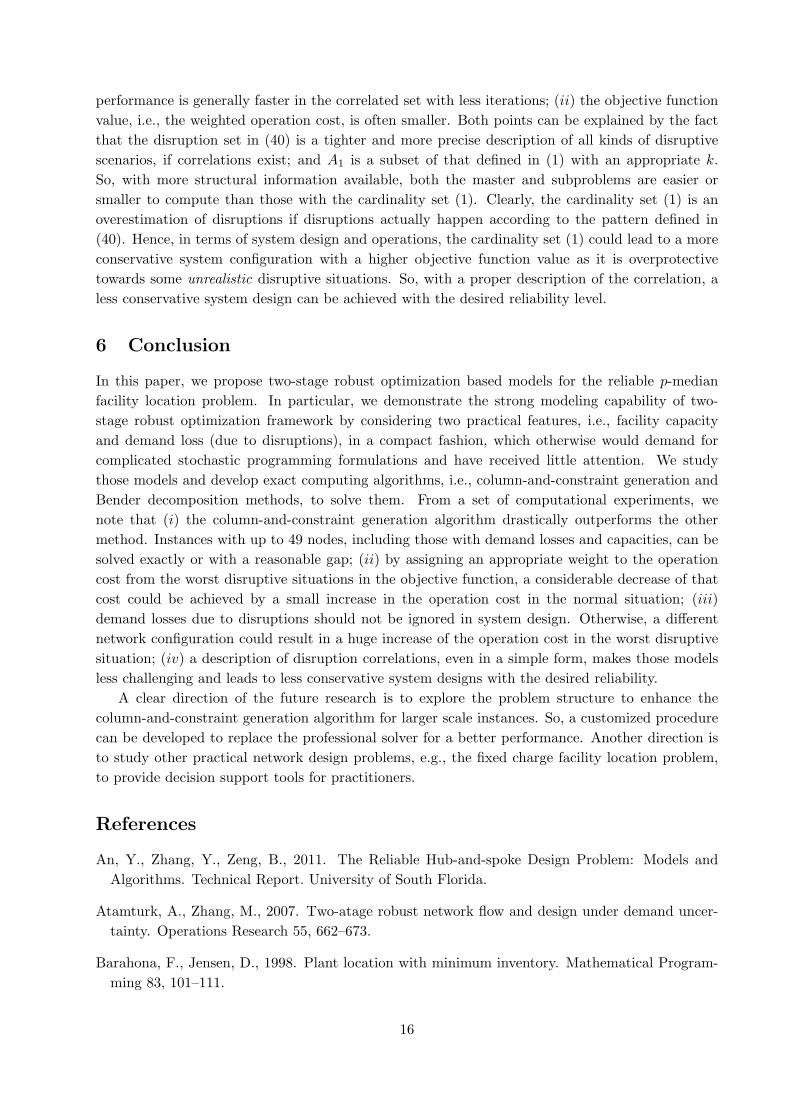
Table 2 presents the performance of the BD methods on instances of RO-PMPl. Table 3 - 6

summarize the computational results of C&CG algorithm on the four reliable models. In those

tables, the column Time(s) presents the computational time in seconds; the column Iter indicates

the number of iterations; the column Obj shows the best objective value ever found; the column

Gap(%) provides the relative gap in percentage if it is larger than ϵ. If an instance can not be solved

due to extensive computation time or lack of memory, we use T or M, respectively, to indicate the

reason in the Time(s) column.

Based on those tables, we observe that

(i) C&CG algorithm performs hundreds of times faster and takes much fewer iterations than the

classical Benders decomposition method. This result confirms the observations made in Zhao

and Zeng (2010) for the robust power system scheduling problem and Zeng and Zhao (2011)

for the location-transportation network design problem. Actually, compared to results in

Zhao and Zeng (2010) and Zeng and Zhao (2011), a more significant superiority of C&CG

algorithm is demonstrated in solving reliable p-median problems.

(ii) The computation complexity of C&CG algorithm increases with the problem size |I| and k,

as well as the weight coefficient ρ. In all four types of models, the most challenging instances

are those with largest |I|, k, and ρ. Note that all instances with k = 1 are easy to compute.

Most small size instances with |I| = 25 can be solved to optimality or with a small optimality

gap while some instances with |I| = 49 are difficult. A closer analysis shows that SP can

be computed easily and the actual bottleneck is to solve MP, which will grow into a large

MIP problem over iterations. As CPLEX, a general-purpose MIP solver, is currently called

to solve MP, one possible direction of future research is to develop a specialized algorithm

that takes advantage of the structure of MP for a faster computation.

(iii) Including additional features does not incur significant computational expense. Compared

with models without capacity restrictions or demand losses, capacitated ones are slightly

harder while models with demand losses could be easier. Hence, our two-stage RO formu-

lations of reliable p-median problems are computationally robust to additional features or

restrictions.

13

(iv) Although for many instances the optimal objective values are the same for the different M

values, the large penalty coefficient M generally negatively impacts the computational per-

formance, which is more significant for instances in capacitated models. One explanation is

that large penalty coefficient M forces demand that was served by a disrupted facility to be

served by survived ones, instead of being simply treated as unmet demand. As a result, the

optimization complexity increases.

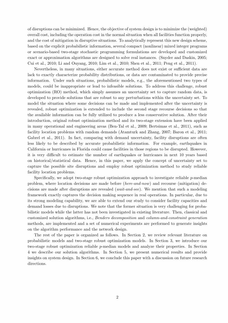
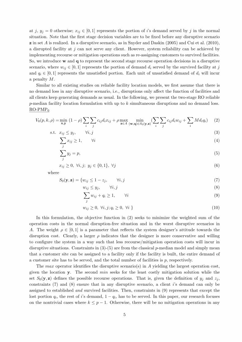
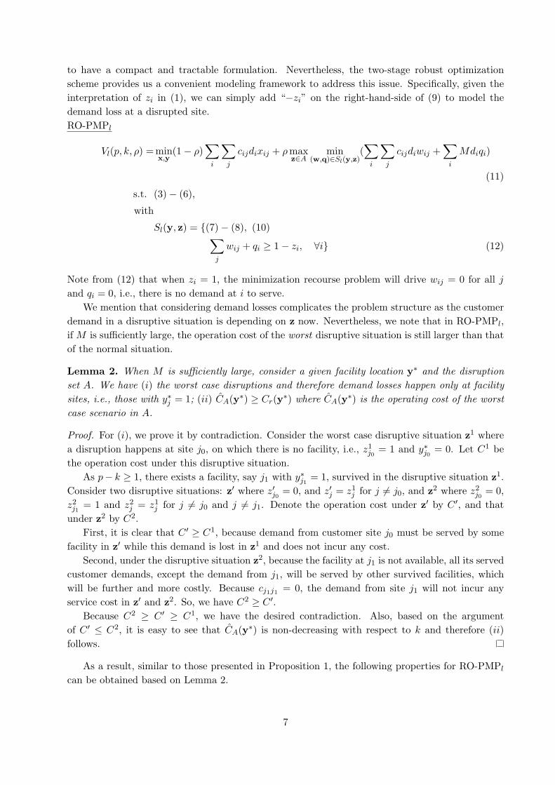
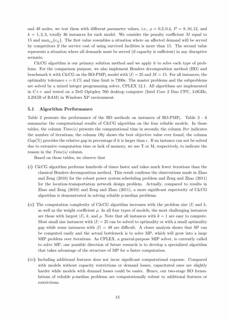
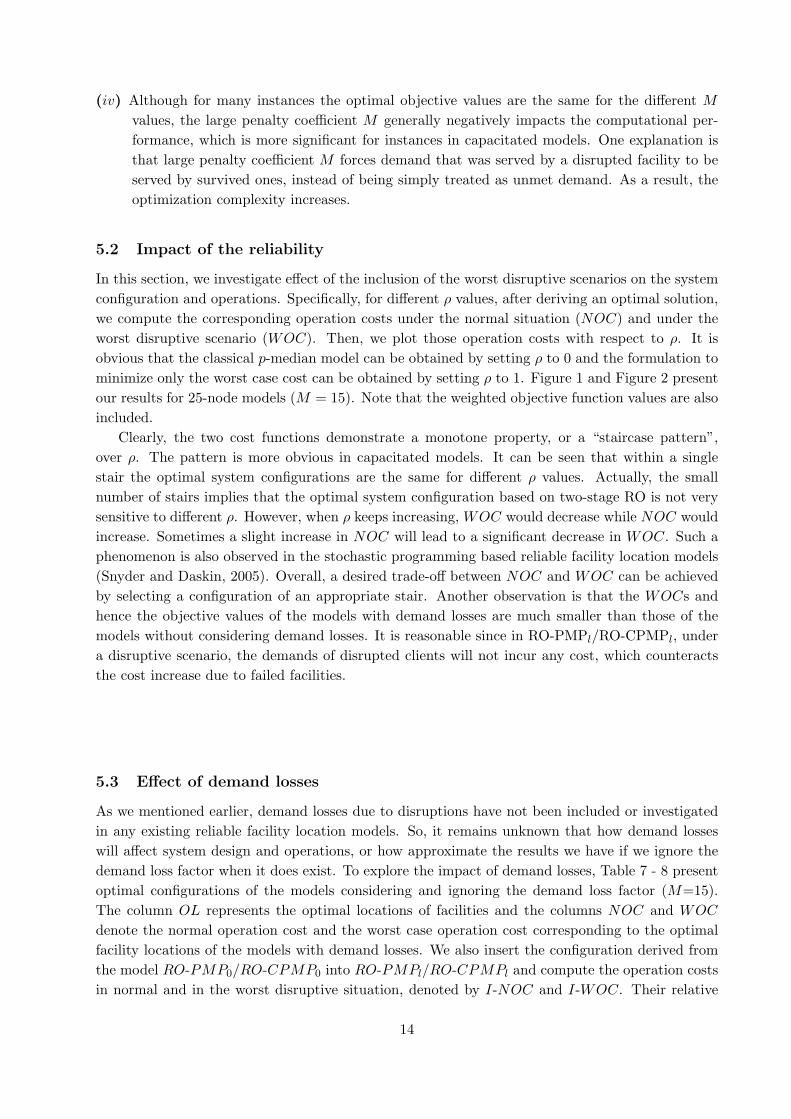
5.2 Impact of the reliability

In this section, we investigate effect of the inclusion of the worst disruptive scenarios on the system

configuration and operations. Specifically, for different ρ values, after deriving an optimal solution,

we compute the corresponding operation costs under the normal situation (NOC) and under the

worst disruptive scenario (WOC). Then, we plot those operation costs with respect to ρ. It is

obvious that the classical p-median model can be obtained by setting ρ to 0 and the formulation to

minimize only the worst case cost can be obtained by setting ρ to 1. Figure 1 and Figure 2 present

our results for 25-node models (M = 15). Note that the weighted objective function values are also

included.

Clearly, the two cost functions demonstrate a monotone property, or a “staircase pattern”,

over ρ. The pattern is more obvious in capacitated models. It can be seen that within a single

stair the optimal system configurations are the same for different ρ values. Actually, the small

number of stairs implies that the optimal system configuration based on two-stage RO is not very

sensitive to different ρ. However, when ρ keeps increasing, WOC would decrease while NOC would

increase. Sometimes a slight increase in NOC will lead to a significant decrease in WOC. Such a

phenomenon is also observed in the stochastic programming based reliable facility location models

(Snyder and Daskin, 2005). Overall, a desired trade-off between NOC and WOC can be achieved

by selecting a configuration of an appropriate stair. Another observation is that the WOCs and

hence the objective values of the models with demand losses are much smaller than those of the

models without considering demand losses. It is reasonable since in RO-PMPl/RO-CPMPl, under

a disruptive scenario, the demands of disrupted clients will not incur any cost, which counteracts

the cost increase due to failed facilities.

5.3 Effect of demand losses

As we mentioned earlier, demand losses due to disruptions have not been included or investigated

in any existing reliable facility location models. So, it remains unknown that how demand losses

will affect system design and operations, or how approximate the results we have if we ignore the

demand loss factor when it does exist. To explore the impact of demand losses, Table 7 - 8 present

optimal configurations of the models considering and ignoring the demand loss factor (M=15).

The column OL represents the optimal locations of facilities and the columns NOC and WOC

denote the normal operation cost and the worst case operation cost corresponding to the optimal

facility locations of the models with demand losses. We also insert the configuration derived from

the model RO-PMP0/RO-CPMP0 into RO-PMPl/RO-CPMPl and compute the operation costs

in normal and in the worst disruptive situation, denoted by I-NOC and I-WOC. Their relative

14

changes with respect to NOC and WOC are denoted by ∆NOC(%) and ∆WOC(%). For a case, if

the optimal facility locations are different for the models with and without demand losses, we will

highlight the locations by underlines.

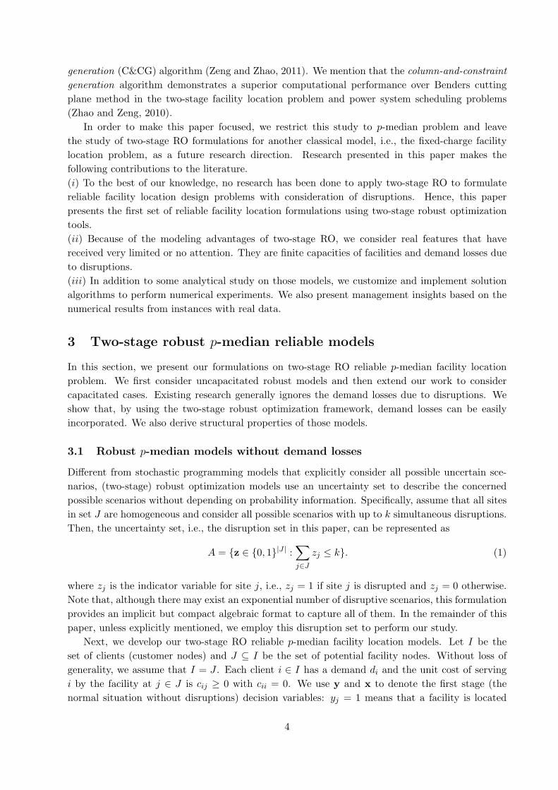
We observe that the demand loss plays a significant role in determining system configuration.

In all 36 instances, including uncapacitated and capacitated ones, there are 18 instances where

optimal facility locations are different from those derived from models ignoring demand losses. In

fact, when we put more weight on the worst disruptive situations, the impact of demand losses

becomes more significant. For example, when ρ = 0.4, there are 11 instances (out of 18 ones) on

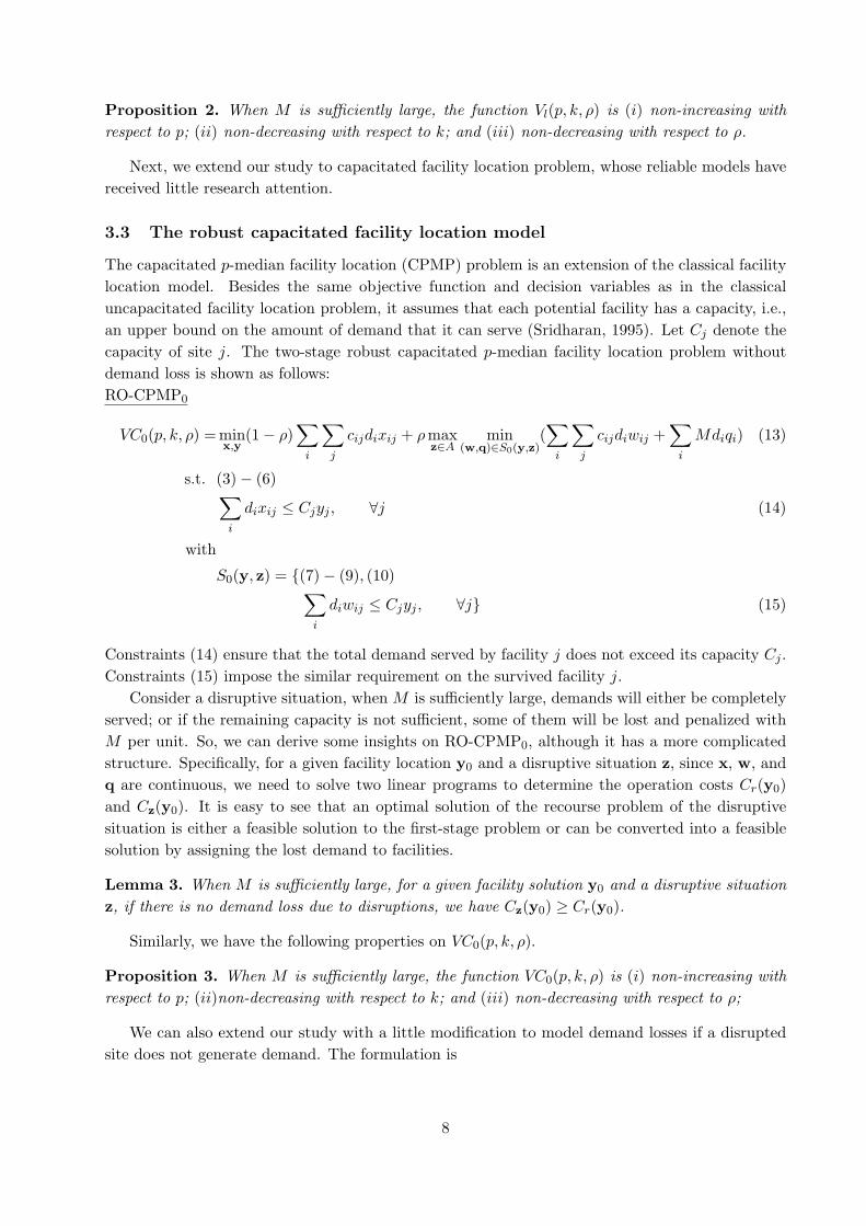
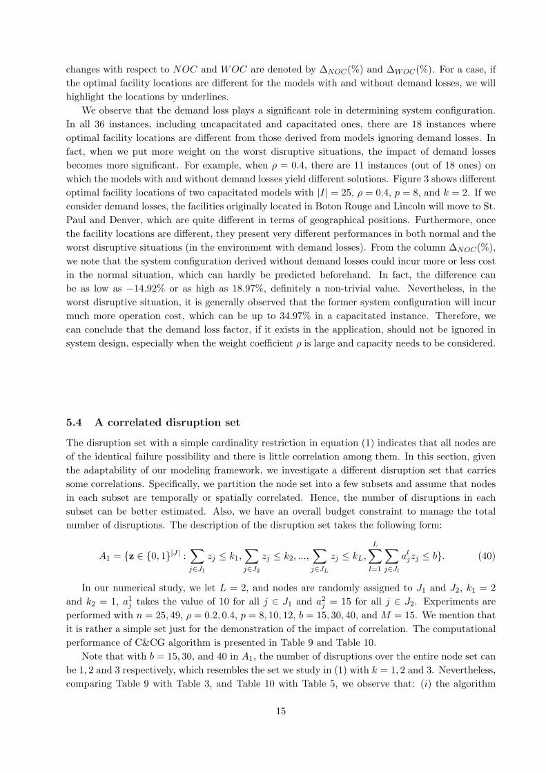
which the models with and without demand losses yield different solutions. Figure 3 shows different

optimal facility locations of two capacitated models with |I| = 25, ρ = 0.4, p = 8, and k = 2. If we

consider demand losses, the facilities originally located in Boton Rouge and Lincoln will move to St.

Paul and Denver, which are quite different in terms of geographical positions. Furthermore, once

the facility locations are different, they present very different performances in both normal and the

worst disruptive situations (in the environment with demand losses). From the column ∆NOC(%),

we note that the system configuration derived without demand losses could incur more or less cost

in the normal situation, which can hardly be predicted beforehand. In fact, the difference can

be as low as −14.92% or as high as 18.97%, definitely a non-trivial value. Nevertheless, in the

worst disruptive situation, it is generally observed that the former system configuration will incur

much more operation cost, which can be up to 34.97% in a capacitated instance. Therefore, we

can conclude that the demand loss factor, if it exists in the application, should not be ignored in

system design, especially when the weight coefficient ρ is large and capacity needs to be considered.

5.4 A correlated disruption set

The disruption set with a simple cardinality restriction in equation (1) indicates that all nodes are

of the identical failure possibility and there is little correlation among them. In this section, given

the adaptability of our modeling framework, we investigate a different disruption set that carries

some correlations. Specifically, we partition the node set into a few subsets and assume that nodes

in each subset are temporally or spatially correlated. Hence, the number of disruptions in each

subset can be better estimated. Also, we have an overall budget constraint to manage the total

number of disruptions. The description of the disruption set takes the following form:

A1 = {z ∈ {0, 1}|J | :∑j∈J1

zj ≤ k1,∑j∈J2

zj ≤ k2, ...,∑j∈JL

zj ≤ kL,

L∑l=1

∑j∈Jl

aljzj ≤ b}. (40)

In our numerical study, we let L = 2, and nodes are randomly assigned to J1 and J2, k1 = 2

and k2 = 1, a1j takes the value of 10 for all j ∈ J1 and a2j = 15 for all j ∈ J2. Experiments are

performed with n = 25, 49, ρ = 0.2, 0.4, p = 8, 10, 12, b = 15, 30, 40, and M = 15. We mention that

it is rather a simple set just for the demonstration of the impact of correlation. The computational

performance of C&CG algorithm is presented in Table 9 and Table 10.

Note that with b = 15, 30, and 40 in A1, the number of disruptions over the entire node set can

be 1, 2 and 3 respectively, which resembles the set we study in (1) with k = 1, 2 and 3. Nevertheless,

comparing Table 9 with Table 3, and Table 10 with Table 5, we observe that: (i) the algorithm

15

performance is generally faster in the correlated set with less iterations; (ii) the objective function

value, i.e., the weighted operation cost, is often smaller. Both points can be explained by the fact

that the disruption set in (40) is a tighter and more precise description of all kinds of disruptive

scenarios, if correlations exist; and A1 is a subset of that defined in (1) with an appropriate k.

So, with more structural information available, both the master and subproblems are easier or

smaller to compute than those with the cardinality set (1). Clearly, the cardinality set (1) is an

overestimation of disruptions if disruptions actually happen according to the pattern defined in

(40). Hence, in terms of system design and operations, the cardinality set (1) could lead to a more

conservative system configuration with a higher objective function value as it is overprotective

towards some unrealistic disruptive situations. So, with a proper description of the correlation, a

less conservative system design can be achieved with the desired reliability level.

6 Conclusion

In this paper, we propose two-stage robust optimization based models for the reliable p-median

facility location problem. In particular, we demonstrate the strong modeling capability of two-

stage robust optimization framework by considering two practical features, i.e., facility capacity

and demand loss (due to disruptions), in a compact fashion, which otherwise would demand for

complicated stochastic programming formulations and have received little attention. We study

those models and develop exact computing algorithms, i.e., column-and-constraint generation and

Bender decomposition methods, to solve them. From a set of computational experiments, we

note that (i) the column-and-constraint generation algorithm drastically outperforms the other

method. Instances with up to 49 nodes, including those with demand losses and capacities, can be

solved exactly or with a reasonable gap; (ii) by assigning an appropriate weight to the operation

cost from the worst disruptive situations in the objective function, a considerable decrease of that

cost could be achieved by a small increase in the operation cost in the normal situation; (iii)

demand losses due to disruptions should not be ignored in system design. Otherwise, a different

network configuration could result in a huge increase of the operation cost in the worst disruptive

situation; (iv) a description of disruption correlations, even in a simple form, makes those models

less challenging and leads to less conservative system designs with the desired reliability.

A clear direction of the future research is to explore the problem structure to enhance the

column-and-constraint generation algorithm for larger scale instances. So, a customized procedure

can be developed to replace the professional solver for a better performance. Another direction is

to study other practical network design problems, e.g., the fixed charge facility location problem,

to provide decision support tools for practitioners.

References

An, Y., Zhang, Y., Zeng, B., 2011. The Reliable Hub-and-spoke Design Problem: Models and

Algorithms. Technical Report. University of South Florida.

Atamturk, A., Zhang, M., 2007. Two-atage robust network flow and design under demand uncer-

tainty. Operations Research 55, 662–673.

Barahona, F., Jensen, D., 1998. Plant location with minimum inventory. Mathematical Program-

ming 83, 101–111.

16

Baron, O., Milner, J., Naseraldin, H., 2011. Facility location: a robust optimization approach.

Production and Operations Management 20, 772–785.

Ben-Tal, A., El Ghaoui, L., Nemirovski, A., 2009. Robust Optimization. Princeton Univ Press.

Ben-Tal, A., Goryashko, A., Guslitzer, E., Nemirovski, A., 2004. Adjustable robust solutions of

uncertain linear programs. Mathematical Programming 99, 351–376.

Berman, O., Krass, D., Menezes, M., 2007. Facility reliability issues in network p-median problems:

strategic centralization and co-location effects. Operations Research 55, 332–350.

Bertsimas, D., Brown, D., Caramanis, C., 2011. Theory and applications of robust optimization.

SIAM Review 53, 464–501.

Bertsimas, D., Litvinov, E., Sun, X., Zhao, J., Zheng, T., 2012. Adaptive robust optimization for

the security constrained unit commitment problem. Power Systems, IEEE Transactions on 99,

1–12.

Cui, T., Ouyang, Y., Shen, Z., 2010. Reliable facility location design under the risk of disruptions.

Operations Research 58, 998–1011.

Daskin, M., 1995. Network and Discrete Location: Models, Algorithms, and Applications. Wiley-

Interscience.

Drezner, E., 1995. Facility Location: A Survey of Applications and Methods. Springer.

Drezner, Z., 1987. Heuristic solution methods for two location problems with unreliable facilities.

Journal of the Operational Research Society 38, 509–514.

Gabrel, V., Lacroix, M., Murat, C., Remli, N., 2011. Robust location transportation problems

under uncertain demands. to appear in Discrete Applied Mathematics .

Gulpınar, N., Pachamanova, D., Canakoglu, E., 2012. Robust strategies for facility location under

uncertainty. European Journal of Operational Research 225, 21–35.

Jia, H., Ordonez, F., Dessouky, M., 2007. A modeling framework for facility location of medical

services for large-scale emergencies. IIE Transactions 39, 41–55.

Jiang, R., Zhang, M., Li, G., Guan, Y., 2011. Benders Decomposition for the Two-stage Security

Constrained Robust Unit Commitment Problem. Technical Report. University of Florida.

Li, Q., Zeng, B., Savachkin, A., 2012. Reliable facility location design under disruptions. To appear

in Computers & Operations Research .

Li, X., Ouyang, Y., 2010. A continuum approximation approach to reliable facility location design

under correlated probabilistic disruptions. Transportation Research Part B 44, 535–548.

Lim, M., Daskin, M., Bassamboo, A., Chopra, S., 2010. A facility reliability problem: Formulation,

properties, and algorithm. Naval Research Logistics 57, 58–70.

Melo, M., Nickel, S., Saldanha-Da-Gama, F., 2009. Facility location and supply chain management-

a review. European Journal of Operational Research 196, 401–412.

17

Peng, P., Snyder, L., Lim, A., Liu, Z., 2011. Reliable logistics networks design with facility disrup-

tions. Transportation Research Part B 45, 1190–1211.

Revelle, C., Eiselt, H., Daskin, M., 2008. A bibliography for some fundamental problem categories

in discrete location science. European Journal of Operational Research 184, 817–848.

Shen, Z., Zhan, R., Zhang, J., 2011. The reliable facility location problem: Formulations, heuristics,

and approximation algorithms. INFORMS Journal on Computing 23, 470–482.

Snyder, L., 2006. Facility location under uncertainty: a review. IIE Transactions 38, 547–564.

Snyder, L., Atan, Z., Peng, P., Rong, Y., Schmitt, A., Sinsoysal, B., 2010. OR/MS models for

supply chainn disruptions: a review. Available at SSRN: http://ssrn.com/abstract=1689882.

Snyder, L., Daskin, M., 2005. Reliability models for facility location: The expected failure cost

case. Transportation Science 39, 400–416.

Sridharan, R., 1995. The capacitated plant location problem. European Journal of Operational

Research 87, 203–213.

Teo, C., Shu, J., 2004. Warehouse-retailer network design problem. Operations Research 52,

396–408.

Zeng, B., Zhao, L., 2011. Solving Two-stage Robust Optimization Problems by A Column-and-

constraint Generation Method. Technical Report. submitted.

Zhao, L., Zeng, B., 2010. Robust Unit Commitment Problem with Demand Response and Wind

Energy. Technical Report. University of South Florida.

18

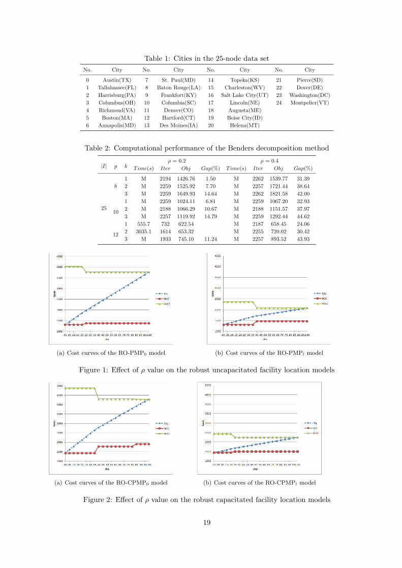
Table 1: Cities in the 25-node data set

No. City No. City No. City No. City

0 Austin(TX) 7 St. Paul(MD) 14 Topeka(KS) 21 Pierre(SD)

1 Tallahassee(FL) 8 Baton Rouge(LA) 15 Charleston(WV) 22 Dover(DE)

2 Harrisburg(PA) 9 Frankfort(KY) 16 Salt Lake City(UT) 23 Washington(DC)

3 Columbus(OH) 10 Columbia(SC) 17 Lincoln(NE) 24 Montpelier(VT)

4 Richmond(VA) 11 Denver(CO) 18 Augusta(ME)

5 Boston(MA) 12 Hartford(CT) 19 Boise City(ID)

6 Annapolis(MD) 13 Des Moines(IA) 20 Helena(MT)

Table 2: Computational performance of the Benders decomposition method

|I| p kρ = 0.2 ρ = 0.4

Time(s) Iter Obj Gap(%) Time(s) Iter Obj Gap(%)

25

8

1 M 2194 1426.76 1.50 M 2262 1539.77 31.39

2 M 2259 1525.92 7.70 M 2257 1721.44 38.64

3 M 2259 1649.93 14.64 M 2262 1821.58 42.00

10

1 M 2259 1024.11 6.81 M 2259 1067.20 32.93

2 M 2188 1066.29 10.67 M 2188 1151.57 37.97

3 M 2257 1119.92 14.79 M 2259 1292.44 44.62

12

1 555.7 732 622.54 M 2187 658.45 24.06

2 3035.1 1614 653.32 M 2255 720.02 30.42

3 M 1933 745.10 11.24 M 2257 893.52 43.93

(a) Cost curves of the RO-PMP0 model (b) Cost curves of the RO-PMPl model

Figure 1: Effect of ρ value on the robust uncapacitated facility location models

(a) Cost curves of the RO-CPMP0 model (b) Cost curves of the RO-CPMPl model

Figure 2: Effect of ρ value on the robust capacitated facility location models

19

Table 3: Computational results for uncapacitated instances with M = 15

|I| ρ p kRO-PMP0 RO-PMPl

Time(s) Iter Obj Gap(%) Time(s) Iter Obj Gap(%)

25

0.2

8

1 1.9 5 1558.09 1.9 5 1426.76

2 4.8 8 1855.51 4.2 7 1525.92

3 T 58 2292.82 0.46 27.3 13 1649.93

10

1 0.8 2 1139.08 3.4 7 1024.11

2 2.0 6 1374.09 10.9 10 1066.29

3 16.4 11 1601.93 6.9 8 1119.92

12

1 0.7 2 811.73 0.5 2 622.54

2 0.7 3 973.46 0.7 2 653.32

3 1.5 3 1110.90 6.1 9 745.10

0.4

8

1 1.9 5 1802.45 5.0 8 1539.77

2 30.3 15 2335.00 40.0 14 1721.44

3 T 84 3194.56 13.69 80.1 17 1821.58

10

1 0.6 2 1364.19 5.2 9 1067.20

2 9.8 10 1785.45 13.4 11 1151.57

3 181.9 23 2235.93 61.8 15 1292.44

12

1 0.7 2 1036.84 1.8 3 658.45

2 1.4 3 1360.29 0.6 3 720.02

3 0.7 3 1635.19 139.1 22 893.52

49

0.2

8

1 9.1 5 6145.54 4.2 2 5684.45

2 187.2 10 6808.88 244.9 10 6020.47

3 T 35 7471.69 9.98 T 29 6364.45 3.26

10

1 3.3 3 4950.32 34.7 6 4687.15

2 617.3 16 5534.76 1050.1 14 4982.95

3 T 27 6106.86 4.80 T 22 5131.20 0.64

12

1 4.6 3 4181.94 3.2 3 3830.82

2 402.9 11 4582.71 56.4 9 4022.75

3 7174.4 25 5011.58 T 20 4217.79 0.27

0.4

8

1 15.5 6 6625.50 32.5 6 5898.97

2 T 28 8326.04 7.60 T 26 6534.28 2.55

3 T 36 9344.74 21.74 T 34 7215.81 13.62

10

1 11.4 5 5351.47 34.5 7 4796.70

2 T 35 6815.54 12.80 T 24 5298.70 1.44

3 T 37 7520.25 15.49 T 34 5827.05 11.91

121 48.8 8 4583.09 7.9 4 3920.28

2 T 26 5397.18 2.35 2577.6 18 4239.83

3 T 39 6249.57 12.98 T 33 4694.21 9.68

20

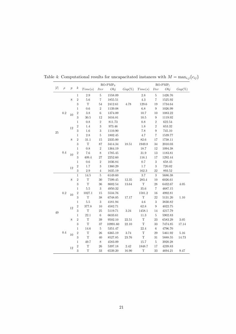
Table 4: Computational results for uncapacitated instances with M = maxi,j{cij}

|I| ρ p kRO-PMP0 RO-PMPl

Time(s) Iter Obj Gap(%) Time(s) Iter Obj Gap(%)

25

0.2

8

1 2.9 5 1558.09 2.8 5 1426.76

2 5.6 7 1855.51 4.3 7 1525.92

3 T 54 2412.61 4.78 129.6 19 1734.64

10

1 0.6 2 1139.08 6.8 9 1026.99

2 3.8 6 1374.09 10.7 10 1083.22

3 30.5 12 1616.81 10.5 9 1119.92

12

1 0.8 2 811.73 0.8 2 622.54

2 1.4 3 973.46 1.8 2 653.32

3 1.6 3 1110.90 7.8 9 745.10

0.4

8

1 2.8 5 1802.45 4.7 7 1539.77

2 31.1 15 2335.00 82.6 17 1738.11

3 T 87 3414.34 18.51 1949.8 34 2010.03

10

1 0.8 2 1364.19 18.7 12 1094.38

2 7.6 8 1785.45 31.9 13 1183.81

3 409.4 27 2252.60 116.1 17 1292.44

12

1 0.6 2 1036.84 0.7 3 658.45

2 1.7 3 1360.29 1.7 3 720.02

3 2.9 4 1635.19 162.3 22 893.52

49

0.2

8

1 14.5 5 6149.60 3.7 3 5686.38

2 T 30 7599.45 12.35 283.4 10 6026.61

3 T 36 8602.54 13.64 T 28 6432.67 4.05

10

1 5.5 3 4950.32 35.6 7 4687.15

2 1027.1 15 5534.76 1581.2 16 4992.81

3 T 38 6748.05 17.17 T 22 5131.20 1.10

12

1 5.5 3 4181.94 4.6 3 3830.82

2 377.8 10 4582.71 62.8 9 4022.75

3 T 25 5119.71 3.24 1458.1 14 4217.79

0.4

8

1 22.1 6 6633.61 11.3 5 5902.83

2 T 39 9502.10 22.51 T 23 6583.29 3.05

3 T 37 10991.60 22.10 T 33 7474.85 17.14

10

1 14.6 5 5351.47 22.4 6 4796.70

2 T 26 6365.19 3.74 T 29 5461.92 5.16

3 T 40 8527.85 23.76 T 31 5888.55 14.73

12

1 49.7 8 4583.09 15.7 5 3920.28

2 T 26 5397.18 2.42 1848.7 17 4239.83

3 T 33 6539.20 16.90 T 33 4694.21 9.47

21

Table 5: Computational results for capacitated instances with M = 15

|I| ρ p kRO-CPMP0 RO-CPMPl

Time(s) Iter Obj Gap(%) Time(s) Iter Obj Gap(%)

25

0.2

8

1 2.9 4 1783.39 2.8 4 1550.58

2 10 6 2126.51 8.5 8 1638.56

3 38.7 10 2466.17 9.7 8 1725.95

10

1 0.5 2 1148.48 1.4 5 1036.93

2 1.7 3 1383.48 4.6 6 1094.58

3 2.9 6 1642.20 10.8 8 1180.54

12

1 0.7 2 821.12 0.7 2 642.54

2 1.9 3 982.85 2.5 5 715.66

3 8.7 8 1266.38 3.9 6 756.96

0.4

8

1 2.9 4 2024.04 2.5 6 1623.29

2 75.9 13 2791.94 23.3 10 1799.26

3 4172 35 3495.95 175.1 18 2015.52

10

1 0.8 2 1373.58 8.7 8 1083.45

2 1.2 3 1843.59 21.3 10 1224.17

3 16.6 8 2307.08 782.4 25 1403.52

12

1 0.4 2 1046.23 1.5 3 689.06

2 1.8 3 1369.69 27.6 12 835.30

3 37.7 16 1828.23 60.8 14 895.72

49

0.2

8

1 10.6 4 6432.77 79.3 6 6180.25

2 T 26 7290.78 10.90 T 19 6525.89 2.01

3 T 27 8302.32 19.43 T 22 7134.59 8.75

10

1 17.2 5 5045.10 23.8 6 4778.10

2 T 23 5752.22 3.06 1262.5 14 5097.14

3 T 20 6187.69 6.55 T 19 5250.64 0.76

12

1 8.3 4 4228.04 4.7 3 3920.98

2 T 18 4797.85 0.76 71.8 8 4104.87

3 T 36 5235.33 8.09 T 21 4379.91 1.60

0.4

8

1 131.5 8 6939.44 502.5 11 6426.95

2 T 31 8677.54 17.51 T 25 7388.72 10.00

3 T 34 10205.90 23.84 T 34 8291.22 17.83

10

1 55.9 7 5434.73 34.9 7 4881.02

2 T 34 6888.70 14.20 T 24 5593.89 6.08

3 T 25 7759.64 15.83 T 24 5885.55 10.76

121 35.0 7 4617.67 9.4 4 4018.48

2 T 23 5399.02 2.68 2794.1 15 4321.95

3 T 41 6647.17 21.97 T 32 4906.77 12.87

22

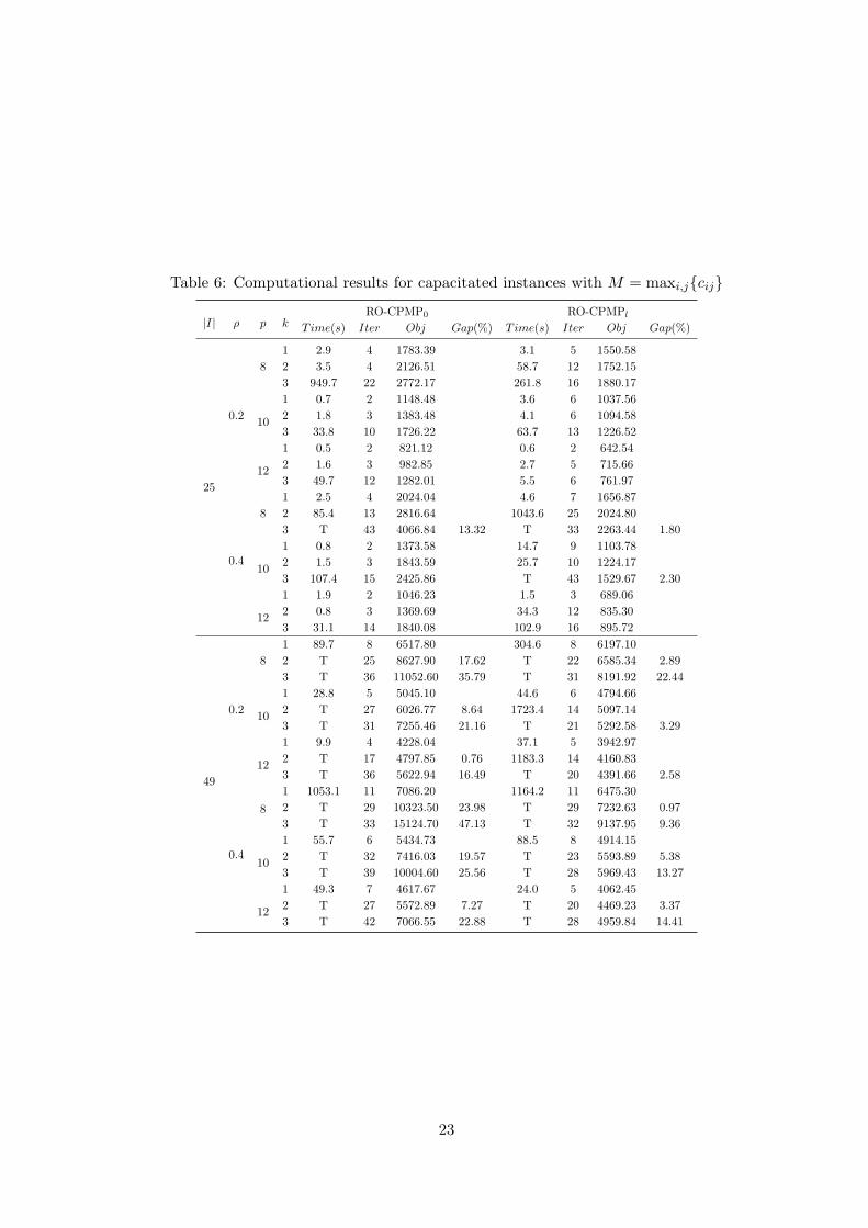
Table 6: Computational results for capacitated instances with M = maxi,j{cij}

|I| ρ p kRO-CPMP0 RO-CPMPl

Time(s) Iter Obj Gap(%) Time(s) Iter Obj Gap(%)

25

0.2

8

1 2.9 4 1783.39 3.1 5 1550.58

2 3.5 4 2126.51 58.7 12 1752.15

3 949.7 22 2772.17 261.8 16 1880.17

10

1 0.7 2 1148.48 3.6 6 1037.56

2 1.8 3 1383.48 4.1 6 1094.58

3 33.8 10 1726.22 63.7 13 1226.52

12

1 0.5 2 821.12 0.6 2 642.54

2 1.6 3 982.85 2.7 5 715.66

3 49.7 12 1282.01 5.5 6 761.97

0.4

8

1 2.5 4 2024.04 4.6 7 1656.87

2 85.4 13 2816.64 1043.6 25 2024.80

3 T 43 4066.84 13.32 T 33 2263.44 1.80

10

1 0.8 2 1373.58 14.7 9 1103.78

2 1.5 3 1843.59 25.7 10 1224.17

3 107.4 15 2425.86 T 43 1529.67 2.30

12

1 1.9 2 1046.23 1.5 3 689.06

2 0.8 3 1369.69 34.3 12 835.30

3 31.1 14 1840.08 102.9 16 895.72

49

0.2

8

1 89.7 8 6517.80 304.6 8 6197.10

2 T 25 8627.90 17.62 T 22 6585.34 2.89

3 T 36 11052.60 35.79 T 31 8191.92 22.44

10

1 28.8 5 5045.10 44.6 6 4794.66

2 T 27 6026.77 8.64 1723.4 14 5097.14

3 T 31 7255.46 21.16 T 21 5292.58 3.29

12

1 9.9 4 4228.04 37.1 5 3942.97

2 T 17 4797.85 0.76 1183.3 14 4160.83

3 T 36 5622.94 16.49 T 20 4391.66 2.58

0.4

8

1 1053.1 11 7086.20 1164.2 11 6475.30

2 T 29 10323.50 23.98 T 29 7232.63 0.97

3 T 33 15124.70 47.13 T 32 9137.95 9.36

10

1 55.7 6 5434.73 88.5 8 4914.15

2 T 32 7416.03 19.57 T 23 5593.89 5.38

3 T 39 10004.60 25.56 T 28 5969.43 13.27

12

1 49.3 7 4617.67 24.0 5 4062.45

2 T 27 5572.89 7.27 T 20 4469.23 3.37

3 T 42 7066.55 22.88 T 28 4959.84 14.41

23

Table 7: Comparison between RO-PMPl and RO-PMP0 models (|I| = 25)

ρ p kRO-PMPl RO-PMP0

OL NOC WOC OL I-NOC I-WOC ∆NOC(%) ∆WOC(%)

0.2

81 0 1 2 3 5 8 11 13 1313.74 1878.84 0 1 2 3 5 8 11 13 1313.74 1878.84 0.00 0.00

2 0 1 2 3 5 8 11 13 1313.74 2374.64 0 1 2 3 5 8 11 13 1313.74 2374.64 0.00 0.00

3 0 1 2 3 4 5 7 11 1478.28 2336.53 0 1 2 3 4 5 11 13 1417.77 2659.42 -4.09 13.82

10

1 0 1 2 3 4 5 7 8 11 14 981.02 1196.49 0 1 2 3 4 5 8 11 13 16 913.98 1479.05 -6.83 23.62

2 0 1 2 3 4 5 7 8 11 14 981.02 1407.39 0 1 2 3 4 5 8 11 13 16 913.98 1764.15 -6.83 25.35

3 0 1 2 3 4 5 8 11 13 16 913.98 1943.70 0 1 2 3 4 5 8 10 11 13 967.93 2132.01 5.90 9.69

121 0 1 2 3 4 5 7 8 10 11 14 16 586.62 766.19 0 1 2 3 4 5 7 8 10 11 14 16 586.62 766.19 0.00 0.00

2 0 1 2 3 4 5 7 8 10 11 14 16 586.62 920.11 0 1 2 3 4 5 7 8 10 11 14 16 586.62 920.11 0.00 0.00

3 0 1 2 3 4 5 7 8 10 11 14 16 586.62 1378.98 0 1 2 3 4 5 7 8 10 11 14 16 586.62 1378.98 0.00 0.00

0.4

81 0 1 2 3 5 8 11 13 1313.74 1878.82 0 1 2 3 5 8 11 13 1313.74 1878.82 0.00 0.00

2 0 1 2 3 4 5 7 11 1478.28 2086.18 0 1 2 3 8 11 12 13 1380.83 2696.66 -6.59 29.26

3 0 1 2 3 4 5 7 11 1478.28 2336.53 0 1 3 5 6 10 11 17 1546.41 2983.21 4.61 27.68

10

1 0 1 2 3 4 5 7 8 11 14 981.02 1196.48 0 1 2 3 4 5 8 11 13 16 913.98 1479.04 -6.83 23.62

2 0 1 2 3 4 5 7 8 11 14 981.02 1407.40 0 1 2 3 4 5 7 8 11 14 981.02 1407.40 0.00 0.00

3 0 1 2 3 4 5 7 8 11 16 974.49 1769.37 0 1 2 3 4 5 8 10 11 13 967.93 2132.02 -0.67 20.50

121 0 1 2 3 4 5 7 8 10 11 14 16 586.62 766.19 0 1 2 3 4 5 7 8 10 11 14 16 586.62 766.19 0.00 0.00

2 0 1 2 3 4 5 7 8 10 11 14 16 586.62 920.11 0 1 2 3 4 5 7 8 10 11 14 16 586.62 920.11 0.00 0.00

3 0 1 2 3 4 5 6 7 8 11 13 16 689.51 1199.54 0 1 2 3 4 5 7 8 10 11 14 16 586.62 1378.98 -14.92 14.96

Table 8: Comparison between RO-CPMPl and RO-CPMP0 models (|I| = 25)

ρ p kRO-CPMPl RO-CPMP0

OL NOC WOC OL I-NOC I-WOC ∆NOC(%) ∆WOC(%)

0.2

81 0 1 2 3 4 5 11 13 1436.38 2007.38 0 1 3 4 5 8 11 13 1518.49 2162.64 5.72 7.73

2 0 1 2 3 4 5 11 13 1436.38 2447.28 0 1 2 3 4 5 11 13 1436.38 2447.28 0.00 0.00

3 0 1 2 3 4 5 11 13 1436.38 2884.23 0 1 2 3 4 5 11 13 1436.38 2884.23 0.00 0.00

10

1 0 1 2 3 4 5 7 8 11 14 990.41 1223.01 0 1 2 3 4 5 8 11 13 16 923.37 1494.32 -6.77 22.18

2 0 1 2 3 4 5 8 11 13 16 923.37 1779.42 0 1 2 3 4 5 8 11 13 16 923.37 1779.42 0.00 0.00

3 0 1 2 3 4 5 8 11 13 16 923.37 2209.22 0 1 2 3 4 5 8 10 11 13 977.33 2183.93 5.84 -1.14

121 0 1 2 3 4 5 7 8 10 11 14 16 596.02 828.62 0 1 2 3 4 5 7 8 10 11 14 16 596.02 828.62 0.00 0.00

2 0 1 2 3 4 5 7 8 10 11 14 16 596.02 1194.22 0 1 2 3 4 5 7 8 10 11 14 16 596.02 1194.22 0.00 0.00

3 0 1 2 3 4 5 7 8 10 11 14 16 596.02 1400.72 0 1 2 3 4 5 7 8 10 11 14 16 596.02 1400.72 0.00 0.00

0.4

81 0 1 2 3 4 5 7 11 1496.89 1812.89 0 1 3 4 8 11 12 13 1573.83 2333.11 5.14 28.70

2 0 1 2 3 4 5 7 11 1496.89 2252.82 0 1 2 3 4 5 8 17 1780.79 3040.72 18.97 34.97

3 0 1 2 3 4 5 11 13 1436.38 2884.23 0 1 2 3 4 5 11 13 1436.38 2884.23 0.00 0.00

10

1 0 1 2 3 4 5 7 8 11 14 990.41 1223.01 0 1 2 3 4 5 8 11 13 16 923.37 1494.35 -6.77 22.19

2 0 1 2 3 4 5 7 8 11 16 983.88 1584.60 0 1 2 3 4 5 8 11 13 16 923.37 1779.45 -6.15 12.30

3 0 1 2 3 4 5 7 8 10 11 1037.84 1952.04 0 1 2 3 4 5 8 10 11 13 977.33 2183.93 -5.83 11.88

121 0 1 2 3 4 5 7 8 10 11 14 16 596.02 828.62 0 1 2 3 4 5 7 8 10 11 14 16 596.02 828.62 0.00 0.00

2 0 1 2 3 4 5 7 8 10 11 14 16 596.02 1194.22 0 1 2 3 4 5 7 8 10 11 14 16 596.02 1194.22 0.00 0.00

3 0 1 2 3 4 5 6 7 8 11 13 16 689.51 1205.04 0 1 2 3 4 5 7 8 9 10 11 14 724.38 1533.51 5.06 27.26

24

(a) System configuration of RO-CPMPl (b) System configuration of RO-CPMP0

Figure 3: Comparison of Optimal Configurations of RO-CPMPl and RO-CPMP0

25

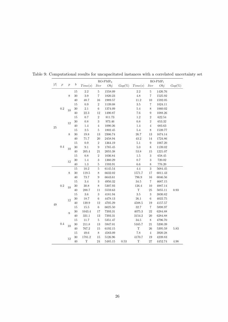
Table 9: Computational results for uncapacitated instances with a correlated uncertainty set

|I| ρ p bRO-PMP0 RO-PMPl

Time(s) Iter Obj Gap(%) Time(s) Iter Obj Gap(%)

25

0.2

8

15 2.2 5 1558.09 2.2 5 1426.76

30 3.9 7 1820.23 4.8 7 1525.92

40 48.7 16 1989.57 11.2 10 1592.05

10

15 0.9 2 1139.08 3.5 7 1024.11

30 2.1 6 1374.09 5.4 8 1060.02

40 22.3 12 1490.87 7.6 9 1088.26

12

15 0.7 2 811.73 1.2 2 622.54

30 0.8 3 973.46 0.8 2 653.32

40 1.4 4 1090.26 1.4 4 683.63

0.4

8

15 2.5 5 1802.45 5.4 8 1539.77

30 19.8 13 2306.74 26.7 13 1674.14

40 71.7 20 2458.94 43.2 14 1724.86

10

15 0.9 2 1364.19 5.1 9 1067.20

30 9.1 9 1785.45 5.0 8 1139.02

40 205.4 21 2055.38 53.8 15 1221.07

12

15 0.8 2 1036.84 1.5 3 658.45

30 1.4 3 1360.29 0.7 3 720.02

40 1.3 5 1593.91 6.6 8 776.20

49

0.2

8

15 10.2 5 6145.54 4.4 3 5684.45

30 119.5 8 6632.02 1571.7 17 6011.43

40 73.7 9 6643.61 796.9 16 6046.56

10

15 3.4 3 4950.32 34.5 7 4687.15

30 30.8 8 5307.93 126.4 10 4887.14

40 288.7 11 5559.63 T 25 5055.11 0.93

12

15 3.6 3 4181.94 3.5 3 3830.82

30 18.7 6 4478.13 26.1 6 4022.75

40 139.9 12 4705.29 4588.5 19 4157.57

0.4

8

15 15.5 6 6625.50 32.7 7 5898.97

30 1043.4 17 7393.31 4075.3 22 6284.88

40 331.1 13 7393.31 3154.2 20 6284.88

10

15 11.7 5 5351.47 34.5 8 4796.70

30 211.8 13 5947.01 5165.7 21 5200.39

40 767.2 15 6192.15 T 26 5395.59 5.83

12

15 49.6 8 4583.09 7.8 4 3920.28

30 1781.2 15 5126.96 4170.7 19 4239.83

40 T 24 5485.15 0.53 T 27 4452.74 4.98

26

Table 10: Computational results for capacitated instances with a correlated uncertainty set

|I| ρ p bRO-CPMP0 RO-CPMPl

Time(s) Iter Obj Gap(%) Time(s) Iter Obj Gap(%)

25

0.2

8

15 2.5 4 1783.39 2.4 4 1550.58

30 2.8 4 2126.51 5.5 6 1597.10

40 26.7 8 2331.96 8.7 8 1626.47

10

15 0.9 2 1148.48 2.6 5 1036.93

30 1.7 3 1383.48 3.4 6 1084.08

40 18.3 10 1612.96 14.5 10 1119.55

12

15 1.6 2 821.12 0.8 2 642.54

30 0.7 3 982.85 2.7 5 715.66

40 49.9 13 1224.47 3.3 6 756.96

0.4

8

15 2.5 4 2024.04 2.8 6 1623.29

30 52.3 12 2791.94 29.7 11 1737.18

40 33.4 10 2895.55 28.8 10 1791.85

10

15 0.9 2 1373.58 9.1 8 1083.45

30 1.7 3 1843.59 28.3 11 1224.17

40 103.8 14 2211.98 48.2 12 1291.03

12

15 0.6 2 1046.23 0.8 3 689.06

30 1.7 3 1369.69 26.4 12 835.30

40 124.5 18 1742.80 100.3 15 882.31

49

0.2

8

15 10.7 4 6432.77 78.3 6 6180.25

30 T 23 7097.47 4.08 1438.4 13 6470.81

40 809.9 11 7062.09 2732.5 16 6470.81

10

15 17.3 5 5045.10 22.5 6 4778.10

30 1293.7 13 5466.82 1535.4 14 5066.65

40 T 22 5898.33 5.79 T 21 5215.26 2.31

12

15 8.4 4 4228.04 4.8 3 3920.98

30 66.0 7 4546.14 47.8 6 4104.87

40 T 19 4833.22 0.93 T 21 4299.91 1.74

0.4

8

15 125.5 8 6939.44 504.5 11 6426.95

30 T 23 7977.01 5.65 T 18 6791.59 1.14

40 5668.7 17 7948.09 1254.8 24 6826.96

10

15 55.5 7 5434.73 33.4 7 4881.02

30 T 30 6276.43 4.55 T 20 5468.66 4.10

40 T 22 6825.37 11.45 T 20 5519.86 5.16

12

15 35.5 7 4617.67 9.7 4 4018.48

30 1564.9 13 5173.96 5312.5 16 4321.95

40 T 23 5531.67 0.20 T 23 4637.33 7.85

27