REMOTE SENSING, GIS AND SCS CURVE NUMBER …€¦ · REMOTE SENSING, GIS AND SCS CURVE NUMBER TECHNIQUES FO R ESTIMATING THE RUNOFF OF PEDDA KEDARI RESERVE FOREST,TEKKALI, SRIK AKULAM,

http://www.iaeme.com/IJCIET/index.asp 428 [email protected]

International Journal of Civil Engineering and Technology (IJCIET) Volume 8, Issue 5, May 2017, pp. 428–443, Article ID: IJCIET_08_05_050 Available online at http://www.iaeme.com/IJCIET/issues.asp?JType=IJCIET&VType=8&IType=5 ISSN Print: 0976-6308 and ISSN Online: 0976-6316 © IAEME Publication Scopus Indexed

REMOTE SENSING, GIS AND SCS CURVE NUMBER TECHNIQUES FOR ESTIMATING

THE RUNOFF OF PEDDA KEDARI RESERVE FOREST,TEKKALI, SRIKAKULAM, AP

Dr. Ch. Kannam Naidu Civil Engineering Department, AITAM-Aditya Institute of Technology and Management,

Tekkali, Andhra Pradesh, India

Dr. Ch. Vasudeva Rao Civil Engineering Department, AITAM-Aditya Institute of Technology and Management,


S. Ramlal Civil Engineering Department, AITAM-Aditya Institute of Technology and Management,


ABSTRACT The primary source of water is rainfall for the generation of runoff over the land

surface. Runoff or overland flow is the flow of water that occurs when excess storm water flows over the earth's surface. Satellite remote sensing and GIS techniques coupled with conventional filed investigations were used for mapping of land use/land cover (LU/LC) features of the study area towards estimating the runoff of the area. The SCS-CN method (SCS, 1985) method involves the use of a simple empirical formula and readily available tables and curves. Determination of SCS curve number depends on the soil and land cover conditions, which the model represents as hydrologic soil group, cover type, treatment and hydrologic condition. Soils are classified into hydrologic soil groups (HSG) to indicate the minimum rate of infiltration obtained for bare soil after prolonged wetting.

Runoff computed from a given rainfall event was integrated with the data of land use treatment, curve numbers and hydrological soil groups by using SCS-CN method. The estimated runoff contributes more than 28% of total rainfall received in the study area. The suitable locations of rainwater harvesting and artificial recharge structures are suggested to increase the groundwater levels for sustainable development of water resources in the Pedda Kedari Reserve Forest. Key words: Runoff, Remote Sensing, GIS, LU/LC, SCS-CN, Hydrologic soil groups.

Remote Sensing, GIS and SCS Curve Number Techniques for Estimating the Runoff of Pedda Kedari Reserve Forest, Tekkali, Srikakulam


Cite this Article: Dr. Ch. Kannam Naidu, Dr. Ch. Vasudeva Rao and S. Ramlal, Remote Sensing, GIS and SCS Curve Number Techniques for Estimating the Runoff of Pedda Kedari Reserve Forest, Tekkali, Srikakulam. International Journal of Civil Engineering and Technology, 8(5), 2017, pp. 428–443. http://www.iaeme.com/IJCIET/issues.asp?JType=IJCIET&VType=8&IType=5

1. INTRODUCTION When rain falls, initially first drops of water are intercepted by the leaves and stems of the vegetation i.e., interception storage. The water reaching the ground surface, as the rain continues, infiltrates into the soil until it reaches a stage where the rate of rainfall exceeds the infiltration capacity of the soil. After that, surface puddles, ditches, tanks and other depressions are filled, thereafter runoff is generated. The infiltration capacity of the soil depends on its texture and on the antecedent soil moisture content (previous rainfall or dry season). The process of runoff generation is continued as long as the rainfall intensity exceeds the actual infiltration capacity of the soil but it stops when the rate of rainfall drops below the actual rate of infiltration.

Remote sensing and GIS have proved an effective means for extracting and processing varied resolutions of spatial information for monitoring natural resources (Masser, 2001). In case of inaccessible region, this technique is perhaps the only method of obtaining the required data on a cost and time-effective basis. Several remote sensing satellites were launched for various purposes and of various resolutions, which provides a new dimension to the remote sensing technology. Now, most common remote sensing systems operates in one and/or several of the visible, infrared, or microwave portions of the electromagnetic spectrum (Jensen, 2007). Digital elevation models (DEM) are among the remote sensing techniques that have been used to measure landscape surface roughness properties over large areas. These are used for visual and mathematical analysis of topography, landscapes and landforms; and also modeling of surface processes (Millaresis and Argialas, 2000; Tucker et al. 2001). Prudhvi Raju and Vaidyanathan (1981) analyzed the fracture patterns of Eastern Ghats region, Andhra Pradesh, which was taken from Landsat imagery using standard visual interpretation techniques. Chetty and Murthy (1993) have mapped the structural and various lithological features of east coast of India using remote sensing data. They adopted different remote sensing techniques for identification of lineaments and other structural features followed by ground check in the field. Land use and land cover changes are important elements of the global environmental change processes (Dickinson, 1995; Hall et al. 1995). Traditional approaches to automated land cover mapping using remotely sensed data have employed pattern recognition techniques including supervised and unsupervised approaches (Jensen, 1986; Benediktsson et al. 1990; Fried and Brodley, 1997; Ward et al. 2000; Rashed et al. 2001; Shamsudheen et al. 2005). Murthy and Venketeswara Rao (1997) have carried out temporal studies of land use/land cover in Varaha river basin, Andhra Pradesh, India using Landsat and IRS LISS data.

Estimating direct runoff depths from storm rainfall by the United States Department of Agriculture (USDA) by curve number (CN) method (Soil Conservation Service (SCS), 1972 and 1985) probably the most widely used techniques. The SCS-CN method is one of the most popular methods for computing the volume of surface runoff in catchments for a given rainfall event. This approach involves the use of a simple empirical formula and readily available tables and curves. A high curve number means high runoff and low infiltration, whereas a low curve number means low runoff and high infiltration. The curve number is a function of land use and hydrologic soil group (HSG). It is a method that can incorporate the land use for computation of runoff from rainfall. The SCS-CN method provides a rapid way

Dr. Ch. Kannam Naidu, Dr. Ch. Vasudeva Rao and S. Ramlal


to estimate runoff change due to land use change (Shrestha, 2003; Zhan and Huang, 2004). The SCS-CN method is a well accepted tool in applied hydrology. Greene and Cruise (1995) and Ponce and Hawkins (1996) worked on the applicability of curve number and considered the CN method as one of the useful tool for calculating runoff depths. Gary and Carmen (2007) conducted a study to ascertain the impact of land use and management practices on rainfall-runoff relationship and used GIS techniques to route runoff through a watershed. The land use/land cover, HSGs and storm rainfall data were utilized to estimate the runoff (Durbude et al. 2001; Ambazhagan et al. 2005; Jasrotia and Singh, 2006; Rao et al. 2010; Kumar and Rajpoot, 2013).High relief and steep slopes impart higher runoff, while the topographical depressions help in an increased infiltration. Surface water bodies like rivers, ponds, etc. can act as recharge zones enhancing the groundwater potential in the vicinity (Jensen, 1986). Geospatial data land use/land cover and Lineaments are not available for Pedda Kedari Reserve Forest area. The topic of the present project work has highest importance and relevance, as the rapid drawing of water resources have enormous impact on the environment of the study area. The focus of the research work is to identify the various factors affecting the water and land environments using geospatial information in Pedda Kedari Reserve Forest area of Srikakulam district, Andhra Pradesh, India.

1.1. Study Area The study area, Pedda Kedari Reserve Forest, is an integral part of Srikakulam district of Andhra Pradesh State. The district is located in the north-eastern part of the State. The district has a coastline of 192 km, and is situated in between the Eastern Ghats and the Bay of Bengal. It is one of the less populated and low literacy district of the State. The district is endowed by good rainfall, forest wealth, mineral and surface water resources. The aerial extent is 5,837 km2. The district is bounded by the Bay of Bengal on the east, Vizianagaram district on west and south, and Odisha state on north and northwest. Howrah–Chennai broad gauge railway line and NH-5 are passing through the district almost parallel to the coastline. The district is divided into three revenue divisions viz. Srikakulam, Palakonda and Tekkali. Further these revenue divisions are subdivided into 38 revenue mandals consisting of six towns and 1,763 villages with a population of 25,37,593 as per Census 2011. The urban population is 4,36,347 whereas rural population constitutes 22,63,124 (District Census Handbook, 2011). The density of population of the district is 462 persons per km2. The important rivers flowing in the district are Vamsadhara, Nagavali, Suvarnamukhi, Vegavati, Mahendratanaya and Bahuda. Among the rivers Vamsadhara, Nagavali and Suvarnamukhi are perennial (Figure 1.0). The general drainage pattern is dendritic to sub-dendritic and occasionally parallel at places.

Figure 1 Location map of the study area



1.2. Data Used and Methodology The survey of India (SOI) toposheet No. 74 B/2 of 1:50,000 along with GeoEye-I imagery of 1.65 m resolution and Landsat ETM+ imagery of 30 m resolution were used to generate the different maps. DEM was generated from the toposheet contour data there by generated Slope map and Aspect map. Land Use/Land Cover was mapped using the GeoEye-I imagery by visual interpretation. Lineaments map was mapped using the Landsat imagery by applying sobel filter techniques. The Soil Texture Map was collected from National Bureau of Soil Sciences (NBSS), Nagpur. The daily rainfall data of Meliaputti was collected for the years of 2005 to 2014. The daily rainfall data has been used for determination of storm events to identify anti moisture conditions.

Flow Chart

2. RESULTS AND DISCUSSIONS Runoff computed from a given rainfall event was integrated with the data of land use treatment, curve numbers and hydrological soil groups by using SCS-CN method. The SCS-CN method (SCS, 1985) method involves the use of a simple empirical formula and readily available tables and curves. A high curve number means high runoff and low infiltration, whereas a low curve number means low runoff and high infiltration. The curve number could be estimated from land use and hydrologic soil group. It is a method that can incorporate the land use for computation of runoff from rainfall. The SCS-CN method provides a rapid way to estimate runoff change due to land use change.

METHODOLOGY

TOPOSHEET (SOI) SATELLITE DATA NBSS DATA RAINFALL DATA

DEM

SLOPE MAP

ASPECT MAP

GEOEYE-I

LANDSAT

LU/LC MAP

LINEAMENTS

SOIL TEXTURE

HSG A HSG D

CURVE NUMBERS

AMC I

AMC II

AMC III

SCS CURVE NUMBER METHOD

RUNOFF ESTIMATION

STREAM NETWORK

CONTOUR DATA

SUGGESTIONS

ARTIFICIAL RECHARGE STRUCTURES RAINWATER HARVESTING STRUCTURES



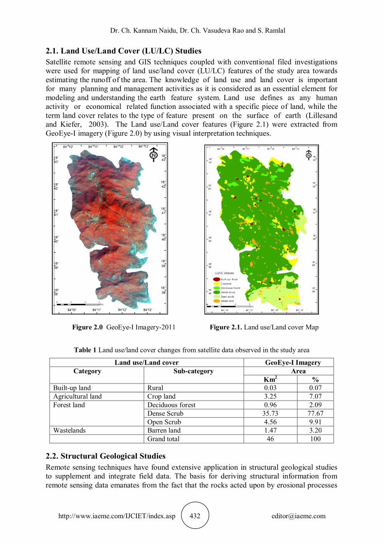
2.1. Land Use/Land Cover (LU/LC) Studies Satellite remote sensing and GIS techniques coupled with conventional filed investigations were used for mapping of land use/land cover (LU/LC) features of the study area towards estimating the runoff of the area. The knowledge of land use and land cover is important for many planning and management activities as it is considered as an essential element for modeling and understanding the earth feature system. Land use defines as any human activity or economical related function associated with a specific piece of land, while the term land cover relates to the type of feature present on the surface of earth (Lillesand and Kiefer, 2003). The Land use/Land cover features (Figure 2.1) were extracted from GeoEye-I imagery (Figure 2.0) by using visual interpretation techniques.

Figure 2.0 GeoEye-I Imagery-2011 Figure 2.1. Land use/Land cover Map

Table 1 Land use/land cover changes from satellite data observed in the study area

Land use/Land cover GeoEye-I Imagery Category Sub-category Area

Km2 % Built-up land Rural 0.03 0.07 Agricultural land Crop land 3.25 7.07 Forest land Deciduous forest 0.96 2.09

Dense Scrub 35.73 77.67 Open Scrub 4.56 9.91

Wastelands Barren land 1.47 3.20 Grand total 46 100

2.2. Structural Geological Studies Remote sensing techniques have found extensive application in structural geological studies to supplement and integrate field data. The basis for deriving structural information from remote sensing data emanates from the fact that the rocks acted upon by erosional processes



result in landforms (Raviprakash Gupta, 1991). Lineament map has been generated from Landsat 7 ETM+ of Band 1, Band 2 and Band 3 using Sobel directional filter. A number of major and minor lineaments traverse the study area. Lineaments appear on the FCC imagery as straight, curvilinear, parallel and discontinuity features. The pattern of lineament is important on the image. Lineaments with straighter alignments indicating moderate to steeply dipping surfaces in the study area. The length and direction of lineaments present in this area vary considerably. The study areas is characterized by major NS, NE-SW and NNE trending lineaments (Figure 2.2) and are varying in length between 0.17 and 1.25 km.

Figure 2.3. Lineaments Map of Study Area

2.3. SCS Curve Number Method Determination of SCS curve number depends on the soil and land cover conditions, which the model represents as hydrologic soil group, cover type, treatment and hydrologic condition. This method is based on an assumption of proportionality between retention and runoff as,

PQ

SQP



Where Q is actual direct runoff, P is total storm rainfall, and S is potential maximum retention.

The retention parameter (S) varies spatially, due to changes in soils, land use and slope and temporally due to changes in soil-water content. This is the ratio of actual retention of rainfall to potential retention is equal to the ratio of actual runoff to rainfall minus initial abstraction. This assumption underscores the conceptual basis of the runoff curve number method expressed as,

a

a

IPQ

SQIP

SIP

IPQ

a

2a

Where P, Q and S are expressed in mm or inches. The initial abstraction Ia is all the losses before runoff begins. It includes the water

retained in surface depressions and the water intercepted by vegetation, evaporation and infiltration. So Ia is highly variable but generally is correlated with soil and cover parameters. After several studies Ia was found to be approximated as,

0.2SIa Substituting Ia in the above equation, we get

1.4............................................ eq0.8S)(P0.2S)(PQ

2

For convenience in evaluating antecedent rainfall, soil conditions, a land use and conservation practice (SCS, 1985) defines:

10

CN100025.4S

CN is an arbitrary curve number varying from 0 to 100.

2.4. Rainfall Data Rainfall data was collected from Meliaputti rain gauge center which is the only one center situated to the nearest for the study area. The recorded daily rainfall data was collected during the period 2005-2014. The daily rainfall data has been used for determination of storm events to identify anti moisture conditions. Precipitation in the study area is mainly concentrated in two rainy seasons, from June to September and October to November. The study area receives about 55% of rainfall from the south-west monsoon during the months of June to September.

2.5. Soil Textural Map The soil map has been collected from National Bureau of Soil Sciences (NBSS). Two types of soil textural classes have been identified and the areal extent of these classes is as follows.

Table 2

S.No Textural Class Area Km2 %

1 Sandy Clay/Clay Loam 34.12 74.2 2 Sandy Loam/Loamy Sand 11.88 25.8



Figure 2.4. Soil Texture Map of Study Area

2.6. Hydrologic Soil Groups (HSG) Soils are classified into hydrologic soil groups to indicate the minimum rate of infiltration obtained for bare soil after prolonged wetting. The HSG are used in determining runoff curve numbers. Infiltration rates of soils vary widely and are affected by subsurface permeability as well as surface intake rates. Soils are classified into four HSG namely A, B, C, and D, according to their minimum infiltration rate, which is obtained for bare soil after prolonged wetting (USDA, 1986). The infiltration rate is the rate at which water enters the soil at the soil surface. Hydrologic soil groups derived based on the textural classes of the soils in the study area are given as follows.

Table 3

HSG A: Soils have low runoff potential and high infiltration rates; HSG D: Soils have high runoff potential. They have very low infiltration rates;

2.7. Curve Number (CN) Values In order to determine the curve number values the land use categories in the study area were considered. Standard SCS curve number values (USDA, 1986) were assigned for each land use and soil group combination. Table 4 presents the curve number values and the corresponding land and soil group combination. The land use classes of the study area are settlements, crop land, forest land, scrub and wastelands and were taken into consideration for the analysis.

Soil Textural Class HSG Area in Km2

Sandy loam/loamy sand A 11.88 Sandy clay/clay loam D 34.12



Table 4 Curve numbers and statistical distribution of land use categories with HSG in the study area

S.No Land use HSG Curve Number (CN)

Area (A) km2

CN*A

1 Settlements A 77 0.02 1.5 D 92 0.03 2.8

2 Crop land A 72 1.73 124.6 D 91 1.50 136.5

3 Forest land A 45 0.20 9.0 D 83 0.80 66.4

4 Scrub A 68 7.73 525.6 D 89 27.92 2484.9

5 Wastelands A 68 2.20 149.6 D 89 3.87 344.4

2.8. Antecedent Moisture Condition (AMC) Antecedent soil moisture condition has an important effect on the runoff. Considering this, SCS developed three antecedent soil moisture conditions such as AMC I AMC II and AMC III. Prior to the estimation of runoff for a storm event, the curve numbers should be adjusted on the basis of the season and 5-day antecedent precipitation. The AMC as described by McCuen (1982) is the initial moisture condition of the soil, prior to the storm event of interest and this parameter is taken as an index based on seasonal limits for the total 5-day antecedent rainfall as follows.

Table 5

AMC class 5-day antecedent rainfall (mm) Dormant season Growing season

I <12.5 <35 II 12.5-27.5 35-52.5 III >27.5 >52.5

The following equation is used for calculating the weighted curve number,

n

1i i

ii

AACNCN

Where CNi = curve number of each land use-hydrologic soil group Ai = area of each land use-hydrologic soil group n = class number of land use-hydrologic soil group

The weighted curve number was computed using the above formula for AMC II condition and the obtained value is 84. CN values for AMC-I and AMC-III can be computed using the following empirical equations (Chow, 1964).

IICN0.05810IICN4.2ICN

IICN0.1310

IICN23IIICN

The weighted curve number obtained from the calculations for AMC-II is 84,

corresponding to this value of the conversion curve numbers for CNI and CNIII are 69 and 92, respectively. The obtained curve number values have been taken into consideration for estimating the potential maximum retention (S) of the soil with water for AMC-II of CNII using the equation as follows.



48.381084

100025.4

10II CN

100025.4S

The calculated values of S is 48.38 for AMC II, 114.12 for AMC I and 22.09 for AMC III

conditions. The obtained S value is substituted in the equation 4.1, to the each storm event for estimating the runoff.

2.9. Runoff Estimation The daily rainfall data for 10 years and also the weighted curve number values in the present study have been taken into the consideration for estimation of runoff using SCS CN method. The runoff is calculated from the different storm events of observed rainfall during the years 2005 to 2014. Estimated runoff for each and every storm event in different AMC conditions for all the years is presented in Table 3.0. The runoff contribution is generally higher during later part of the monsoon months that has been resulted as higher observed runoff. If the storm event rainfall is less than 25 mm, then it was not considered for determination of runoff because it does not contribute any runoff. Most of the major storm events occurred in the months of September and October. The highest precipitation occurs during cyclonic storms, which results in peak flows in the local drainage. Such cyclonic storms are very common during late July, August, September and October months. The average annual runoff in the study area was estimated to be 389.8 mm which corresponds to about 28.6% of average annual rainfall of the study area. It was also observed from the data, the runoff varies widely from 11% (2011) to 53.9% (2014). The linear diagram (Figure 6) represents the annual rainfall-runoff relationship during 2005-2014, which is indicating that the overall increase in runoff and decrease in the rainfall trend of the study region. Most of the major storm events occurred in the months of September and October. The highest precipitation occurs during cyclonic storms, which results in peak flows in the local drainage.

Table 6 Runoff estimation for each storm event during the period from 2005-2014 Date of storm-event

Storm Rainfall

(P) mm 5 day total antecedent

rainfall (mm)

AMC Class

Storm runoff (Q)

mm % 17.04.2005-18.04.2005 71.4 0.0 I 14.51 20.32 24.07.2005-26.07.2005 71.4 38.8 II 34.60 48.46 08.08.2005-14.08.2005 185.8 13.0 I 95.86 51.59 01.10.2005-03.10.2005 58.8 34.4 I 8.63 14.67 22.10.2005-23.10.2005 30.2 0.0 I 0.45 1.48 01.11.2005-03.11.2005 77.2 27.2 I 17.55 22.73 15.03.2006-17.03.2006 43.8 5.8 I 3.26 7.44 25.04.2006-26.04.2006 26.2 0.0 I 0.10 0.37 16.05.2006-17.05.2006 34.0 7.2 I 1.00 2.93 27.05.2006-29.05.2006 60.6 65.2 III 40.32 66.54 04.06.2006-06.06.2006 62.2 0.0 I 10.10 16.24 22.06.2006-25.06.2006 50.8 20.2 I 5.51 10.85 28.06.2006-05.07.2006 380.8 15.6 I 271.45 71.28 01.08.2006-04.08.2006 178.2 27.2 I 89.59 50.27 11.08.2006-17.08.2006 113.6 16.4 I 40.22 35.41 21.08.2006-30.08.2006 106.2 9.6 I 35.20 33.15 04.09.2006-05.09.2006 40.0 13.2 I 2.25 5.62 15.09.2006-21.09.2006 90.6 0.0 I 25.26 27.88 29.09.2006-30.09.2006 71.0 0.0 I 14.30 20.15



28.10.2006-30.10.2006 49.6 0.0 I 5.09 10.26 21.06.2007-30.06.2007 286.5 19.2 I 184.04 64.24 19.07.2007-21.07.2007 63.1 0.0 I 10.51 16.65 02.08.2007-08.08.2207 127.4 5.8 I 50.01 39.26 02.09.2007-06.09.2007 93.6 5.2 I 27.10 28.95 10.09.2007-18.09.2007 102.0 61.4 III 79.57 78.01 20.09.2007-24.09.2007 111.8 21.6 I 38.98 34.87 09.02.2008-11.02.2008 43.8 0.0 I 3.26 7.44 24.03.2008-25.03.2008 29.6 0.0 I 0.38 1.28 27.05.2008-28.05.2008 41.2 6.8 I 2.55 6.19 22.06.2008-23.06.2008 63.0 1.0 I 10.46 16.61 11.07.2008-14.07.2008 32.2 23.6 I 0.71 2.21 18.07.2008-21.07.2008 82.6 35.8 II 43.84 53.07 27.07.2008-29.07.2008 76.4 84.4 III 55.08 72.09 02.08.2008-04.08.2008 108.8 33.4 I 36.95 33.96 07.08.2008-10.08.2008 104.7 108.8 III 82.18 78.49 16.08.2008-17.08.2008 89.4 0.0 I 24.53 27.44 05.09.2008-07.09.2008 87.0 2.0 I 23.10 26.56 09.09.2008-18.09.2008 214.6 87.0 III 190.19 88.63 22.09.2008-23.09.2008 57.6 34.6 I 8.12 14.10 12.07.2009-16.07.2009 90.2 3.6 I 25.02 27.73 18.07.2009-22.07.2009 90.4 84.6 III 68.41 75.67 15.08.2009-16.08.2009 55.6 10.8 I 7.32 13.16 25.08.2009-26.08.2009 81.0 23.8 I 19.65 24.26 01.10.2009-04.10.2009 132.2 28.6 I 53.53 40.49 03.04.2010-06.04.2010 166.2 0.0 I 79.84 48.04 13.06.2010-14.06.2010 36.6 0.0 I 1.48 4.06 18.06.2010-21.06.2010 43.0 36.6 II 13.59 31.60 01.07.2010-02.07.2010 96.8 6.2 I 29.10 30.06 05.07.2010-08.07.2010 48.4 96.8 III 29.28 60.49 20.07.2010-22.07.2010 25.2 15.4 I 0.05 0.19 28.07.2010-30.07.2010 42.8 26.2 II 13.46 31.45 03.08.2010-06.08.2010 119.0 12.6 I 43.99 36.97 26.08.2010-28.08.2010 82.8 10.4 I 20.67 24.96 03.09.2010-09.09.2010 120.4 1.0 I 44.98 37.36 24.09.2010-26.09.2010 83.8 0.0 I 21.24 25.34 06.10.2010-09.10.2010 51.0 9.4 I 5.58 10.94 15.10.2010-18.10.2010 163.4 18.6 I 77.60 47.49 30.10.2010-02.11.2010 88.0 6.2 I 23.70 26.93 08.11.2010-09.11.2010 77.0 0.0 I 17.44 22.65 06.12.2010-10.12.2010 125.8 0.0 I 48.85 38.83 20.05.2011-21.05.2011 40.8 0.0 I 2.45 6.00 12.06.2011-14.06.2011 66.8 0.0 I 12.24 18.32 25.06.2011-26.06.2011 71.0 0.0 I 14.30 20.15 05.07.2011-08.07.2011 101.0 25.2 I 31.79 31.47 30.07.2011-02.08.2011 143.2 4.0 I 61.80 43.16 17.09.2011-18.09.2011 37.6 26.4 II 10.22 27.17 21.06.2012-22.06.2012 76.6 0.0 I 17.23 22.49 01.07.2012-04.07.2012 48.0 64.6 III 28.92 60.25 03.08.2012-06.08.2012 44.0 23.0 I 3.32 7.54 01.09.2012-06.09.2012 210.4 0.0 I 116.63 55.43 02.09.2012-04.09.2012 45.6 48.0 III 26.80 58.78 08.09.2012-10.09.2012 57.2 45.6 III 37.21 65.05 18.09.2012-19.09.2012 46.2 10.6 I 3.98 8.61 24.09.2012-26.09.2012 42.6 32.4 I 2.92 6.86 01.10.2012-03.10.2012 34.6 44.4 II 8.47 24.49 23.04.2013-25.04.2013 49.4 56.2 III 30.17 61.06 11.06.2013-13.06.2013 75.8 18.4 I 16.80 22.16



23.06.2013-24.06.2013 44.8 20.2 I 3.55 7.92 14.07.2013-16.07.2013 31.2 74.4 III 14.68 47.04 19.07.2013-22.07.2013 101.2 31.2 I 31.92 31.54 04.08.2013-06.08.2013 83.4 0.0 I 21.01 25.19 11.10.2013-12.10.2013 41.0 0.6 I 2.50 6.09 21.10.2013-27.10.2013 507.2 0.0 I 392.03 77.29 20.11.2013-22.11.2013 27.2 0.0 I 0.16 0.60 25.05.2014-27.05.2014 158.6 0.0 I 73.78 46.52 15.07.2014-16.07.2014 65.2 42.2 II 29.67 45.50 18.07.2014-22.07.2014 65.8 67.4 III 45.14 68.60 28.07.2014-06.08.2014 89.2 0.0 I 24.41 27.37 15.08.2014-19.08.2014 137.6 58.2 III 114.23 83.02 21.08.2014-23.08.2014 52.8 111.2 III 33.21 62.91 28.08.2014-07.09.2014 240.2 52.8 III 215.58 89.75 04.09.2014-07.09.2014 161.4 58.6 III 137.62 85.26 18.09.2014-20.09.2014 33.6 26.2 I 0.93 2.77 11.10.2014-14.10.2014 201.0 0.0 I 108.62 54.04

Such cyclonic storms are very common during late July, August, September and October months. The average annual runoff in the study area was estimated to be 389.8 mm which corresponds to about 28.6% of average annual rainfall of the study area (Table 7). It was also observed from the data, the runoff varies widely from 11% (2011) to 53.9% (2014). The linear diagram (Figure 2.5) represents the annual rainfall-runoff relationship during 2005-2014, which is indicating that the overall increase in runoff and decrease in the rainfall trend of the study region.

Table 7 Trends in rainfall and runoff in the study area

Year Rainfall Runoff mm %

2005 1304.6 171.6 13.2 2006 1740.0 543.7 31.2 2007 1299.6 391.0 30.1 2008 1446.8 473.2 32.7 2009 992.10 173.9 17.5 2010 1626.2 470.8 29.0 2011 1210.6 132.8 11.0 2012 1214.6 245.5 20.2 2013 1343.4 512.8 38.2 2014 1453.8 783.2 53.9

Average 1363.2 389.8 28.6



Figure 2.5. The linear diagram represents trends in rainfall and runoff during 2005-2014

3. SUGGESTIONS The suitable locations for rainwater harvesting (RH) structures are suggested by using the maps of slope, Lineaments, Drainage network. The suitable locations of RH structure are located geographically where lineament meets the drainage network at the slope greater than 250 (Table 8, Figure 3.0). These locations are for artificial recharge (AR) structures (Table 8, Figure 3.0). And separately the locations for the artificial recharge geographically where drainage network meets the foot of the hill (Table 8, Figure 3.0).

Table 8

S.No Latitude Longitude Structure (s) 1 18°38'54.305"N 84°11'15.486"E RH AND AR STRUCTURES 2 18°38'25.214"N 84°12'21.726"E RH AND AR STRUCTURES 3 18°39'08.168"N 84°11'36.484"E RH AND AR STRUCTURES 4 18°39'01.413"N 84°11'20.994"E RH AND AR STRUCTURES 5 18°39'24.902"N 84°11'58.240"E RH AND AR STRUCTURES 6 18°39'58.023"N 84°12'13.823"E RH AND AR STRUCTURES 7 18°40'20.839"N 84°12'18.685"E RH AND AR STRUCTURES 8 18°40'14.378"N 84°12'16.496"E RH AND AR STRUCTURES 9 18°40'28.496"N 84°12'23.129"E RH AND AR STRUCTURES 10 18°40'11.435"N 84°11'19.658"E RH AND AR STRUCTURES 11 18°40'45.023"N 84°12'24.156"E RH AND AR STRUCTURES 12 18°41'08.810"N 84°12'07.867"E RH AND AR STRUCTURES 13 18°40'42.501"N 84°10'58.468"E RH AND AR STRUCTURES 14 18°40'53.439"N 84°11'01.317"E RH AND AR STRUCTURES 15 18°41'13.212"N 84°10'42.543"E RH AND AR STRUCTURES 16 18°41'43.599"N 84°10'03.043"E RH AND AR STRUCTURES 17 18°41'48.106"N 84°12'12.339"E RH AND AR STRUCTURES 18 84°12'12.339"N 84°11'52.014"E RH AND AR STRUCTURES

Runoff

Runoff (in mm

) Rain

fall

(in m

m)



19 18°42'56.054"N 84°11'54.258"E RH AND AR STRUCTURES 20 18°43'15.516"N 84°10'06.293"E RH AND AR STRUCTURES 21 18°43'18.617"N 84°11'28.971"E RH AND AR STRUCTURES 22 18°37'59.323"N 84°12'32.246"E AR STRUCTURE 23 18°38'47.425"N 84°11'4.201"E AR STRUCTURE 24 18°39'56.129"N 84°12'34.055"E AR STRUCTURE 25 18°39'51.956"N 84°12'31.081"E AR STRUCTURE 26 18°40'47.513"N 84°13'5.505"E AR STRUCTURE 27 18°41'44.503"N 84°12'54.710"E AR STRUCTURE 28 18°42'00.902"N 84°12'28.477"E AR STRUCTURE 29 18°42'20.868"N 84°12'25.641"E AR STRUCTURE 30 18°42'20.233"N 84°12'22.551"E AR STRUCTURE 31 18°43'22.398"N 84°12'29.531"E AR STRUCTURE 32 18°43'10.858"N 84°11'52.219"E AR STRUCTURE 33 18°43'23.802"N 84°11'36.490"E AR STRUCTURE 34 18°43'38.796"N 84°11'04.340"E AR STRUCTURE 35 18°43'38.882"N 84°10'20.667"E AR STRUCTURE 36 18°43'23.730"N 84°09'58.487"E AR STRUCTURE 37 18°42'50.968"N 84°09'55.993"E AR STRUCTURE 38 18°42'32.375"N 84° 9' 52.726"E AR STRUCTURE 39 18°42'26.068"N 84°09'53.241"E AR STRUCTURE 40 18°42'13.701"N 84°09'57.625"E AR STRUCTURE 41 18°40'14.604"N 84°10'56.318"E AR STRUCTURE 42 18°40'8.376"N 84°11'22.959"E AR STRUCTURE

Figure 3.0. Suitable locations for Rainwater Harvesting and Artificial Recharge structures



REFERENCES [1] Ambazhagan, S., Ramaswamy, S.M. and Das Gupta, S., 2005, Remote sensing and GIS

for artificial recharge study, runoff estimation and planning in Ayyar basin, Tamil Nadu, India. Environ. Geol. Vol. 48, No. 2, pp. 158-170.

[2] Benediktsson, J., Swain, P. and Ersoy, O.K., 1990, Neural network appro-aches versus statistical methods in classification of multi-source Remote sensing data. IEEE Trans. Geosci. Remote Sensing. Vol. 28, pp. 540-552.

[3] Chetty, T.R.K. and Murthy, D.S.N., 1993, Landsat-thematic mapper data applied to structural studies of the Eastern Ghat granulite terrain in part of Andhra Pradesh. Jour. Geol. Soc. India. Vol. 42, pp. 373-391.

[4] Dickinson, R., 1995, Land processes in climate models. Remote sensing environ, Vol. 51, pp. 27-38.

[5] District Census Handbook: Srikakulam, 2011, Directorate of Census Operations, Andhra Pradesh, Series-29, Part XII-B.

[6] Durbude, D.G., Purandara, B.K. and Sharma, A., 2001, Estimation of surface runoff potential of a watershed in semi arid environment – a case study. Jour. Indian Soc. Remote Sensing, Vol. 29, No. 1&2, pp. 48-58.

[7] Fried, M.A. and Brodley, C.E., 1997, Decision tree classification of land cover from remotely sensed data. Remote sensing environ., Vol. 61, pp. 399-409.

[8] Gary W.C and Carmen Vega., 2007, Impacts of land use changes on runoff generation in the east branch of the Brandywine creek watershed using a GIS-based hydrologic model. Middle states geographer, Vol. 40, pp. 142-149.

[9] Greene, R.G and Cruise, J.F., 1995: Urban watershed modeling using GIS, Journal of Water Resources Planning and Management, ASCE. Vol. 121 No. 4, pp. 318-325.

[10] Hall, F.G., Townsend, J.R. and Engman, E.T., 1995, Status of Remote sensing algorithms for estimation of land surface state parameters. Remote sensing environ., Vol. 51, pp. 138-156.

[11] Jasrotia, A.S. and Singh, R., 2006, Modeling runoff and soil erosion in a catchment area, using the GIS, in the Himalayan region, India. Environ. Geol. Vol. 51, pp. 29-37.

[12] Jensen, J.R., 1986, Introductory digital image processing: a Remote sensing perspective. Prentice Hall, New Jersy.

[13] Jensen, J.R., 2007, Remote sensing of the environment. 1st edition, Dorling Kindersley (India) Pvt. Ltd., New Delhi.

[14] Kumar, A. and Rajpoot, P.S., 2013, Assessment of hydro-environmental loss as surface runoff using CN method of Pahuj river basin datia, India. Proceedings of the international academy of ecology and environmental sciences. Vol. 3, No. 4, pp. 324-329.

[15] Lillesand, T.M. and Kiefer, R.W., 2003, Remote sensing and image interpretation. 4th edition. John Wiley & Sons., New York.

[16] Masser, I., 2001, Managing our urban future: the role of Remote sensing and Geographic information systems. Habitat Int. Vol. 25, pp. 503-512.

[17] McCuen, R.H., 1982, A Guide to hydrologic analysis using SCS methods. Prentice-Hall Inc., Englewood Cliffs, New Jersey.

[18] Millaresis, G.C. and Argialas, D.P., 2000, Extraction and delineation of alluvial fans from digital elevation models and Landsat thematic mapper images. Photogrammetric engg. Remote sensing, Vol. 66, pp. 1093-1101.



[19] Murthy, K.S.R. and Venkateswara Rao, V., 1997, Temporal studies of land use/land cover in Varaha river basin, Andhra Pradesh, India. Jour. Indian Soc. Remote sensing, Vol. 25 No. 3, pp. 145-154.

[20] Ponce, V.M. and Hawkins, R.H., 1996, Runoff curve number: Has it reached maturity?, J. Hydrol. Eng. ASCE. Vol. 1, pp. 11–18.

[21] Rao, K.N., Naredra, K. and Latha, P.S., 2010, An Integrated study of geospatial information technologies for surface runoff estimation in an agricultural watershed, India. J. Indian Soc. Remote Sens. Vol. 38, pp. 255–267.

[22] Rashed, T., Weeks, J.R., Gadalla, M.S. and Hill, A.G., 2001, Revealing the anatomy of cities through spectral mixture analysis of multispectral satellite imagery: a case study of the Greater Cairo region, Egypt. Geocarto Int. Vol. 16, pp. 5-15.

[23] Ravi Prakash Gupta, 1991, Remote Sensing Geology, Geological applications, Springer, Chapter-16, pp. 223-309.

[24] SCS., 1985, Hydrology national engineering handbook, Supplement A, Section 4 Chapter 10, Soil Conservation service. USDA, Washington, DC.

[25] Shamsudheen, M., Dasog, G.S. and Tejaswini, N.B., 2005, Land use/land cover mapping in the coastal area of north Karnataka using remote sensing data. Jour. Indian Soc. Remote Sensing. Vol. 33 No. 2, pp. 253-257.

[26] Shrestha, M.N., 2003, spatially distributed hydrological modeling considering land-use changes using Remote Sensing and GIS. Map asia conference.

[27] Tucker, G.E., Catani, F., Rinaldo, A. and Bras, R.L., 2001, Statistical analysis of drainage density from digital terrain data. Geomorphology, Vol. 36, pp. 187-202.

[28] USDA., 1986, Urban hydrology for small watersheds. Technical release 55 (TR-55). United States department of agriculture, Washington, D.C.

[29] Ward, D., Phinn, S.R., and Murray, A.L., 2000, Monitoring growth in rapidly urbanizing areas using remotely sensed data. Professional geogra. Vol. 53, pp. 371-386.

[30] Zhan, X.Y., and Huang, M.L., 2004, ArcCN-Runoff: An ArcGIS tool for generating curve number and runoff maps. Environmental modeling & software, Vol. 19, pp. 875-879.

[31] A. Manikanta Sai, K. Sanjeev Rahul, B. Mohanty and SS. Asadi, Estimation Analysis of Runoff for Udaygiri Mandal Using A Potential Method: A Model Study. International Journal of Civil Engineering and Technology, 8(4), 2017, pp. 2062-2068

Documents

REMOTE SENSING, GIS AND SCS CURVE NUMBER …€¦ · REMOTE SENSING, GIS AND SCS CURVE NUMBER TECHNIQUES FO R ESTIMATING THE RUNOFF OF PEDDA KEDARI RESERVE FOREST,TEKKALI, SRIK AKULAM,