Remote Sensing Image Analysis with R · landsat

Remote Sensing Image Analysis with R

Aniruddah Ghosh and Robert J. Hijmans

Feb 20, 2019

CONTENTS

1 Introduction 31.1 Terminology . . . . . . . . . . . . . . . . . . . . . . . . . . . . . . . . . . . . . . . . . . . . . . . 31.2 Data . . . . . . . . . . . . . . . . . . . . . . . . . . . . . . . . . . . . . . . . . . . . . . . . . . . . 41.3 Resources . . . . . . . . . . . . . . . . . . . . . . . . . . . . . . . . . . . . . . . . . . . . . . . . . 41.4 R packages . . . . . . . . . . . . . . . . . . . . . . . . . . . . . . . . . . . . . . . . . . . . . . . . 4

2 Exploration 52.1 View image properties . . . . . . . . . . . . . . . . . . . . . . . . . . . . . . . . . . . . . . . . . . 52.2 Image information and statistics . . . . . . . . . . . . . . . . . . . . . . . . . . . . . . . . . . . . . 62.3 Visualize single and multi-band imagery . . . . . . . . . . . . . . . . . . . . . . . . . . . . . . . . 72.4 Subset and rename spectral bands . . . . . . . . . . . . . . . . . . . . . . . . . . . . . . . . . . . . 102.5 Spatial subset or crop . . . . . . . . . . . . . . . . . . . . . . . . . . . . . . . . . . . . . . . . . . . 112.6 Saving results to disk . . . . . . . . . . . . . . . . . . . . . . . . . . . . . . . . . . . . . . . . . . . 112.7 Relation between bands . . . . . . . . . . . . . . . . . . . . . . . . . . . . . . . . . . . . . . . . . 122.8 Extract raster values . . . . . . . . . . . . . . . . . . . . . . . . . . . . . . . . . . . . . . . . . . . 142.9 Spectral profiles . . . . . . . . . . . . . . . . . . . . . . . . . . . . . . . . . . . . . . . . . . . . . 14

3 Basic mathematical operations 173.1 Vegetation indices . . . . . . . . . . . . . . . . . . . . . . . . . . . . . . . . . . . . . . . . . . . . 173.2 Histogram . . . . . . . . . . . . . . . . . . . . . . . . . . . . . . . . . . . . . . . . . . . . . . . . 173.3 Thresholding . . . . . . . . . . . . . . . . . . . . . . . . . . . . . . . . . . . . . . . . . . . . . . . 203.4 Principal component analysis . . . . . . . . . . . . . . . . . . . . . . . . . . . . . . . . . . . . . . 24

4 Unsupervised Image Classification 294.1 kmeans classification . . . . . . . . . . . . . . . . . . . . . . . . . . . . . . . . . . . . . . . . . . . 29

5 Supervised Image Classification 335.1 Reference data . . . . . . . . . . . . . . . . . . . . . . . . . . . . . . . . . . . . . . . . . . . . . . 335.2 Generate sample sites . . . . . . . . . . . . . . . . . . . . . . . . . . . . . . . . . . . . . . . . . . 345.3 Extract cell values for the sample sites . . . . . . . . . . . . . . . . . . . . . . . . . . . . . . . . . . 365.4 Train the classifier using training samples . . . . . . . . . . . . . . . . . . . . . . . . . . . . . . . . 365.5 Classify . . . . . . . . . . . . . . . . . . . . . . . . . . . . . . . . . . . . . . . . . . . . . . . . . . 365.6 Model evaluation . . . . . . . . . . . . . . . . . . . . . . . . . . . . . . . . . . . . . . . . . . . . . 38

i

ii


Aniruddha Ghosh and Robert J. Hijmans

CONTENTS 1


2 CONTENTS

CHAPTER

ONE

INTRODUCTION

This book provides a short introduction to satellite data analysis with R. Before reading this you should first learn thebasics of the raster package.

Getting satellite images for a specific project remains a challenging task. You have to find data that is suitable foryour objectives, and that you can get access to. Important properties to consider while searching the remotely sensed(satellite) data include:

1. Spatial resolution

2. Temporal resolution, including the return time; availability of historical images, and for a particular moment intime)

3. Spectral resolution, that is, the parts of the electromagnetic spectrum (wavelengths) that are sensed

4. Radiometric resolution (sensor sensitivity; ability to measure small differences)

5. Quality (e.g. the presence of cloud-cover or of artefacts in the data (read about problems in Landsat ETM+)

There are numerous sources of remotely sensed data from satellites. Generally, the very high spatial resolution datais available as (costly) commercial products. Lower spatial resolution data is freely available from NASA, ESA andother missions. In this tutorial we’ll use freely available Landsat 8, Landsat 7, Landsat 5, Sentinel and MODIS data.The Landsat program started in 1972 and is is the longest running Earth-observation satellite program.

You can access public satellite data from several sources, including:

i. http://earthexplorer.usgs.gov/

ii. https://lpdaacsvc.cr.usgs.gov/appeears/

iii. https://search.earthdata.nasa.gov/search

iv. https://lpdaac.usgs.gov/data_access/data_pool

v. https://scihub.copernicus.eu/

vi. https://aws.amazon.com/public-data-sets/landsat/

This web site lists 15 sources of freely available remote sensing data.

It is possible to download some satellite data using R-packages. You can use the MODIS or MODISTools package tosearch, download and pre-process different MODIS products.

1.1 Terminology

Most remote sensing products consist of observations of reflectance data. That is, they are measures of the intensityof the sun’s radiation that is reflected by the earth. Reflectance is normally measured for different wavelengths of theelectromagnetic spectrum. For example, it can be measured in the red, green, and blue wavelengths. If that is the case,a satellite image can be referred to as a “multi-spectral” (or hyper-spectral if there are many separate wavelengths).

3

http://rspatial.org/spatial/

http://www.nrcan.gc.ca/node/9407

http://www.seos-project.eu/modules/remotesensing/remotesensing-c03-p05.html

http://www.seos-project.eu/modules/remotesensing/remotesensing-c03-p03.html

http://landsat.usgs.gov/products_slcoffbackground.php

https://landsat.gsfc.nasa.gov/landsat-8/



https://earth.esa.int/web/sentinel/user-guides/sentinel-2-msi

https://lpdaac.usgs.gov/dataset_discovery/modis/modis_products_table

https://landsat.gsfc.nasa.gov/a-landsat-timeline/

http://earthexplorer.usgs.gov/

https://lpdaacsvc.cr.usgs.gov/appeears/

https://search.earthdata.nasa.gov/search

https://lpdaac.usgs.gov/data_access/data_pool

https://scihub.copernicus.eu/

https://aws.amazon.com/public-data-sets/landsat/

http://gisgeography.com/free-satellite-imagery-data-list/

https://cran.r-project.org/web/packages/MODIS/index.html

https://cran.r-project.org/web/packages/MODISTools/index.html

https://lpdaac.usgs.gov/dataset_discovery/modis/modis_products_table


Therefore, a single ‘satellite image’ typically consists of a number of separate raster layers. In remote sensing jargon,these layers are referred to as “bands” (shorthand for “bandwidth”). Other commonly used jargon in remote sensingcircles is “pixel”, which is equivalent to “grid cell”.

1.2 Data

You can download all the data required for the examples used in this book here. Unzip the file contents and save thedata to the R working directory of your computer.

You can also use the below script to download the data.

dir.create('data', showWarnings = FALSE)if (!file.exists('data/rs/samples.rds')) {

download.file('https://biogeo.ucdavis.edu/data/rspatial/rsdata.zip', dest = 'data/→˓rsdata.zip')

unzip('data/rsdata.zip', exdir='data')}

1.3 Resources

Here is a short list of some good resources to learn about remote sensing image analysis:

• Remote Sensing Digital Image Analysis

• Introductory Digital Image Processing: A Remote Sensing Perspective

• A survey of image classification methods and techniques for improving classification performance

• A Review of Modern Approaches to Classification of Remote Sensing Data

• Online remote sensing course

1.4 R packages

Here is a list of some R packages for analyzing remote sensing data:

• RStoolbox

• landsat

• hsdar

• rasterVis for visualization

4 Chapter 1. Introduction

https://biogeo.ucdavis.edu/data/rspatial/rsdata.zip

http://www.springer.com/us/book/9783642300615

https://www.pearsonhighered.com/program/Jensen-Introductory-Digital-Image-Processing-A-Remote-Sensing-Perspective-4th-Edition/PGM30020.html

http://www.tandfonline.com/doi/pdf/10.1080/01431160600746456

http://link.springer.com/chapter/10.1007%2F978-94-007-7969-3_9

http://nptel.ac.in/courses/105108077/

https://cran.r-project.org/web/packages/RStoolbox/index.html

https://cran.r-project.org/web/packages/landsat/index.html

https://cran.r-project.org/web/packages/hsdar/index.html

https://cran.r-project.org/web/packages/rasterVis/index.html

CHAPTER

TWO

EXPLORATION

In this chapter we describe how to access and explore attributes of remote sensing images with R. We also show howto plot (make maps).

We will primarily use a spatial subset of Landsat 8 scene collected on June 14, 2017. The subset covers the areabetween Concord and Stockton, in California, USA.

All Landsat image scenes have a unique product ID and metadata. You can find the information on Landsat sensor,satellite, location on Earth (WRS path, WRS row) and acquisition date from the product ID. For example, the productidentifier of the data we will use is ‘LC08_044034_20170614’. Based on this guide, you can see that the Sensor-Satellite is OLI/TIRS combined Landsat 8, WRS Path 44, WRS Row 34 and collected on June 14, 2017. Landsatscenes are most commonly delivered as zipped file, which contains separate files for the reflectance values at eachbandwidth (wavelength).

We will start by exploring and visualizing the data (See [chapter 1] for data downloading instructions if you have notalready done so).

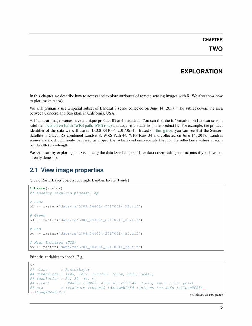
2.1 View image properties

Create RasterLayer objects for single Landsat layers (bands)

library(raster)## Loading required package: sp

# Blueb2 <- raster('data/rs/LC08_044034_20170614_B2.tif')

# Greenb3 <- raster('data/rs/LC08_044034_20170614_B3.tif')

# Redb4 <- raster('data/rs/LC08_044034_20170614_B4.tif')

# Near Infrared (NIR)b5 <- raster('data/rs/LC08_044034_20170614_B5.tif')

Print the variables to check. E.g.

b2## class : RasterLayer## dimensions : 1245, 1497, 1863765 (nrow, ncol, ncell)## resolution : 30, 30 (x, y)## extent : 594090, 639000, 4190190, 4227540 (xmin, xmax, ymin, ymax)## crs : +proj=utm +zone=10 +datum=WGS84 +units=m +no_defs +ellps=WGS84→˓+towgs84=0,0,0

(continues on next page)

5

https://landsat.usgs.gov/what-worldwide-reference-system-wrs

https://landsat.usgs.gov/landsat-collections#Prod%20IDs


(continued from previous page)

## source : c:/github/rspatial/rspatial-web/source/rs/_R/data/rs/LC08_044034_→˓20170614_B2.tif## names : LC08_044034_20170614_B2## values : 0.0748399, 0.7177562 (min, max)

You can see the spatial resolution, extent, number of layers, coordinate reference system and more.

2.2 Image information and statistics

The below shows how you can access various properties from a Raster* object (this is the same for any raster data set).

# coordinate reference system (CRS)crs(b2)## CRS arguments:## +proj=utm +zone=10 +datum=WGS84 +units=m +no_defs +ellps=WGS84## +towgs84=0,0,0

# Number of rows, columns, or cellsncell(b2)## [1] 1863765dim(b2)## [1] 1245 1497 1

# spatial resolutionres(b2)## [1] 30 30

# Number of bandsnlayers(b2)## [1] 1

# Do the bands have the same extent, number of rows and columns, projection,→˓resolution, and origincompareRaster(b2,b3)## [1] TRUE

You can create a RasterStack (an object with multiple layers) from the existing RasterLayer (single band) objects.

landsatRGB <- stack(b4, b3, b2)landsatFCC <- stack(b5, b4, b3)

# Check the properties of the RasterStacklandsatRGB## class : RasterStack## dimensions : 1245, 1497, 1863765, 3 (nrow, ncol, ncell, nlayers)## resolution : 30, 30 (x, y)## extent : 594090, 639000, 4190190, 4227540 (xmin, xmax, ymin, ymax)## crs : +proj=utm +zone=10 +datum=WGS84 +units=m +no_defs +ellps=WGS84→˓+towgs84=0,0,0## names : LC08_044034_20170614_B4, LC08_044034_20170614_B3, LC08_044034_→˓20170614_B2## min values : 0.02084067, 0.04259216, 0.→˓07483990## max values : 0.7861769, 0.6924697, 0.→˓7177562

6 Chapter 2. Exploration


Notice the order of the layers. These are suitable for plotting different color composites. You can learn more aboutcolor composites in remote sensing here and also in the section below.

You can also create the RasterStack using the filenames.

# first create a list of raster layers to usefilenames <- paste0('data/rs/LC08_044034_20170614_B', 1:11, ".tif")filenames## [1] "data/rs/LC08_044034_20170614_B1.tif"## [2] "data/rs/LC08_044034_20170614_B2.tif"## [3] "data/rs/LC08_044034_20170614_B3.tif"## [4] "data/rs/LC08_044034_20170614_B4.tif"## [5] "data/rs/LC08_044034_20170614_B5.tif"## [6] "data/rs/LC08_044034_20170614_B6.tif"## [7] "data/rs/LC08_044034_20170614_B7.tif"## [8] "data/rs/LC08_044034_20170614_B8.tif"## [9] "data/rs/LC08_044034_20170614_B9.tif"## [10] "data/rs/LC08_044034_20170614_B10.tif"## [11] "data/rs/LC08_044034_20170614_B11.tif"

landsat <- stack(filenames)landsat## class : RasterStack## dimensions : 1245, 1497, 1863765, 11 (nrow, ncol, ncell, nlayers)## resolution : 30, 30 (x, y)## extent : 594090, 639000, 4190190, 4227540 (xmin, xmax, ymin, ymax)## crs : +proj=utm +zone=10 +datum=WGS84 +units=m +no_defs +ellps=WGS84→˓+towgs84=0,0,0## names : LC08_044034_20170614_B1, LC08_044034_20170614_B2, LC08_044034_→˓20170614_B3, LC08_044034_20170614_B4, LC08_044034_20170614_B5, LC08_044034_20170614_→˓B6, LC08_044034_20170614_B7, LC08_044034_20170614_B8, LC08_044034_20170614_B9, LC08_→˓044034_20170614_B10, LC08_044034_20170614_B11## min values : 9.641791e-02, 7.483990e-02, 4.→˓259216e-02, 2.084067e-02, 8.457669e-04, -7.872183e-→˓03, -5.052945e-03, 3.931751e-02, -4.337332e-04,→˓ 2.897978e+02, 2.885000e+02## max values : 0.73462820, 0.71775615, 0.→˓69246972, 0.78617686, 1.01243150, 1.04320455,→˓ 1.11793602, 0.82673049, 0.03547901,→˓ 322.43139648, 317.99530029

Above we created a RasterStack with 11 layers. The layers represent reflection intensity in the following wavelengths:Ultra Blue, Blue, Green, Red, Near Infrared (NIR), Shortwave Infrared (SWIR) 1, Shortwave Infrared (SWIR) 2,Panchromatic, Cirrus, Thermal Infrared (TIRS) 1, Thermal Infrared (TIRS) 2. We won’t use the last four layers andwe will learn how to remove those in following sections.

2.3 Visualize single and multi-band imagery

You can plot individual layers of a RasterStack of a multi-spectral image.

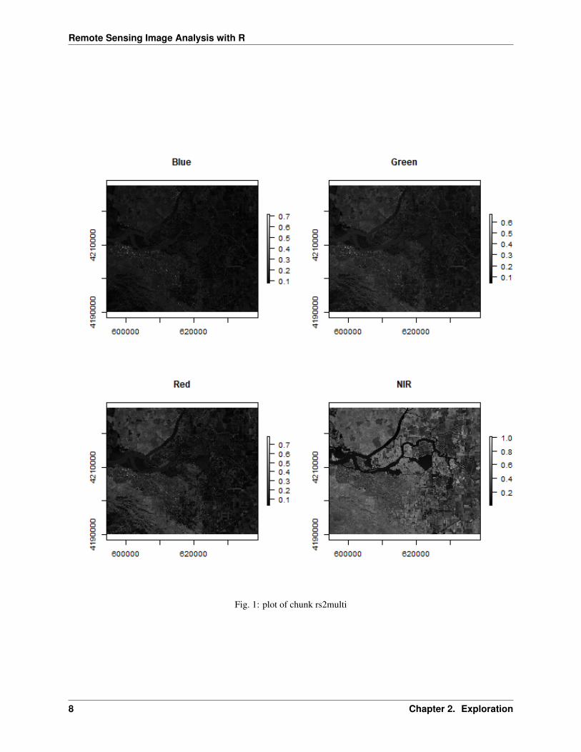
par(mfrow = c(2,2))plot(b2, main = "Blue", col = gray(0:100 / 100))plot(b3, main = "Green", col = gray(0:100 / 100))plot(b4, main = "Red", col = gray(0:100 / 100))plot(b5, main = "NIR", col = gray(0:100 / 100))

Check the legends. They represent the range of values in each layer, and they range from 0 and 1. Notice the differencein shading and range of legends between the different bands. This is because different Earth surface features reflect

2.3. Visualize single and multi-band imagery 7

https://crisp.nus.edu.sg/~research/tutorial/opt_int.htm


Fig. 1: plot of chunk rs2multi



the incident solar radiation differently. Each layer represent how much incident solar radiation is reflected for thatparticular wavelength. For example, vegetation reflects more energy in NIR than other wavelengths and thus appearsbrighter in NIR wavelength. However water absorbs most of the incident energy in NIR regions and appears dark.

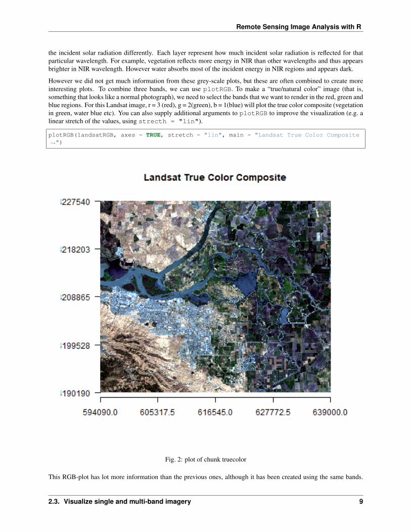
However we did not get much information from these grey-scale plots, but these are often combined to create moreinteresting plots. To combine three bands, we can use plotRGB. To make a “true/natural color” image (that is,something that looks like a normal photograph), we need to select the bands that we want to render in the red, green andblue regions. For this Landsat image, r = 3 (red), g = 2(green), b = 1(blue) will plot the true color composite (vegetationin green, water blue etc). You can also supply additional arguments to plotRGB to improve the visualization (e.g. alinear stretch of the values, using strecth = "lin").

plotRGB(landsatRGB, axes = TRUE, stretch = "lin", main = "Landsat True Color Composite→˓")

Fig. 2: plot of chunk truecolor

This RGB-plot has lot more information than the previous ones, although it has been created using the same bands.

2.3. Visualize single and multi-band imagery 9


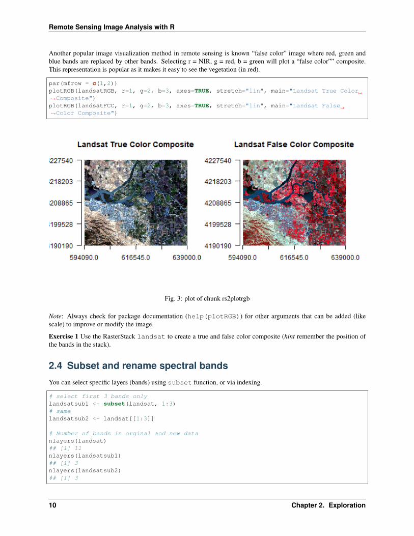
Another popular image visualization method in remote sensing is known “false color” image where red, green andblue bands are replaced by other bands. Selecting r = NIR, g = red, b = green will plot a “false color”” composite.This representation is popular as it makes it easy to see the vegetation (in red).

par(mfrow = c(1,2))plotRGB(landsatRGB, r=1, g=2, b=3, axes=TRUE, stretch="lin", main="Landsat True Color→˓Composite")plotRGB(landsatFCC, r=1, g=2, b=3, axes=TRUE, stretch="lin", main="Landsat False→˓Color Composite")

Fig. 3: plot of chunk rs2plotrgb

Note: Always check for package documentation (help(plotRGB)) for other arguments that can be added (likescale) to improve or modify the image.

Exercise 1 Use the RasterStack landsat to create a true and false color composite (hint remember the position ofthe bands in the stack).

2.4 Subset and rename spectral bands

You can select specific layers (bands) using subset function, or via indexing.

# select first 3 bands onlylandsatsub1 <- subset(landsat, 1:3)# samelandsatsub2 <- landsat[[1:3]]

# Number of bands in orginal and new datanlayers(landsat)## [1] 11nlayers(landsatsub1)## [1] 3nlayers(landsatsub2)## [1] 3



As mentioned above, we have no use here for the last four bands inlandsat. You can remove those using

landsat <- subset(landsat, 1:7)

Set the names of the bands using the following:

names(landsat)## [1] "LC08_044034_20170614_B1" "LC08_044034_20170614_B2"## [3] "LC08_044034_20170614_B3" "LC08_044034_20170614_B4"## [5] "LC08_044034_20170614_B5" "LC08_044034_20170614_B6"## [7] "LC08_044034_20170614_B7"names(landsat) <- c('ultra-blue', 'blue', 'green', 'red', 'NIR', 'SWIR1', 'SWIR2')names(landsat)## [1] "ultra.blue" "blue" "green" "red" "NIR"## [6] "SWIR1" "SWIR2"

2.5 Spatial subset or crop

Spatial subsetting can be used to limit analysis to a geographic subset of the image. Spatial subsets can be created withthe crop function, using an extent object, or another spatial object from which an Extent can be extracted/created,.

# Using extentextent(landsat)## class : Extent## xmin : 594090## xmax : 639000## ymin : 4190190## ymax : 4227540e <- extent(624387, 635752, 4200047, 4210939)

# crop landsat by the extentlandsatcrop <- crop(landsat, e)

Exercise 2 Interactive selection from the image is also possible. Use drawExtent and drawPoly to select an areaof interest. Note: drawing will not work for plots generated within the markdown document. Please run the plot anddraw commands from the RStudio console.

Exercise 3 Use the RasterStack landsatcrop to create a true and false color composite (hint remember the positionof the bands in the stack).

2.6 Saving results to disk

At this stage we may want to save the raster to disk using the function writeRaster. Multiple file types aresupported. We will use the commonly used GeoTiff format. While the layer order is preserved, layer names areunfortunately lost in the GeoTiff format.

writeRaster(landsatcrop,filename = "cropped-landsat.tif", overwrite = TRUE)

To keep the layer names, you can used the ‘raster-grd’ format:

writeRaster(landsatcrop, filename = "cropped-landsat.grd", overwrite = TRUE)

The disadvantage of this format is that not many other programs can read the data, in contrast to the GeoTiff format.

Note: Check for package documentation (help(writeRaster)) for additional helpful arguments that can beadded.

2.5. Spatial subset or crop 11


2.7 Relation between bands

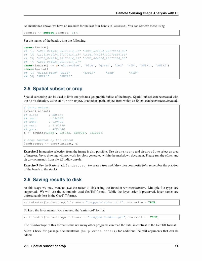
A scatterplot matrix can be helpful in exploring relationships between raster layers. This can be done with the pairs()function of the raster package.

Plot of reflection in the ultra-blue wavelength against reflection in the blue wavelength.

pairs(landsatcrop[[1:2]], main = "Ultra-blue versus Blue")

Fig. 4: plot of chunk rs2pairs1

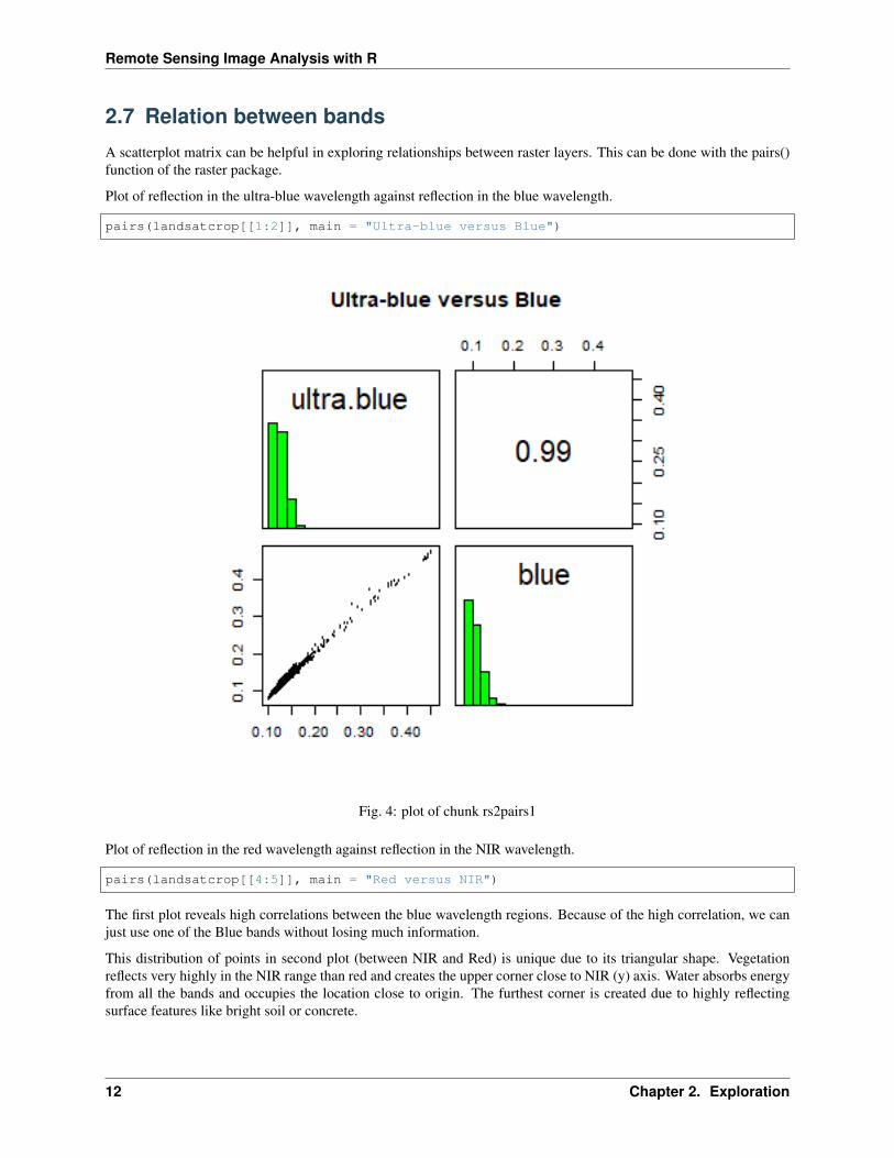
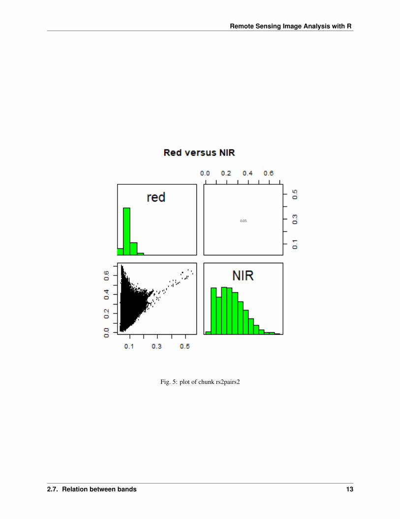
Plot of reflection in the red wavelength against reflection in the NIR wavelength.

pairs(landsatcrop[[4:5]], main = "Red versus NIR")

The first plot reveals high correlations between the blue wavelength regions. Because of the high correlation, we canjust use one of the Blue bands without losing much information.

This distribution of points in second plot (between NIR and Red) is unique due to its triangular shape. Vegetationreflects very highly in the NIR range than red and creates the upper corner close to NIR (y) axis. Water absorbs energyfrom all the bands and occupies the location close to origin. The furthest corner is created due to highly reflectingsurface features like bright soil or concrete.



Fig. 5: plot of chunk rs2pairs2

2.7. Relation between bands 13


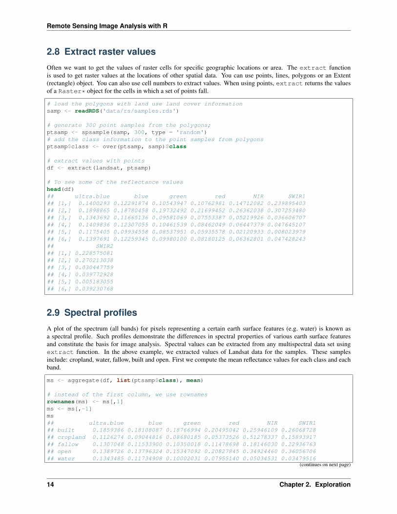
2.8 Extract raster values

Often we want to get the values of raster cells for specific geographic locations or area. The extract functionis used to get raster values at the locations of other spatial data. You can use points, lines, polygons or an Extent(rectangle) object. You can also use cell numbers to extract values. When using points, extract returns the valuesof a Raster* object for the cells in which a set of points fall.

# load the polygons with land use land cover informationsamp <- readRDS('data/rs/samples.rds')

# generate 300 point samples from the polygons;ptsamp <- spsample(samp, 300, type = 'random')# add the class information to the point samples from polygonsptsamp$class <- over(ptsamp, samp)$class

# extract values with pointsdf <- extract(landsat, ptsamp)

# To see some of the reflectance valueshead(df)## ultra.blue blue green red NIR SWIR1## [1,] 0.1400293 0.12291874 0.10543947 0.10762981 0.14712082 0.239895403## [2,] 0.1898865 0.18780458 0.19732492 0.21699452 0.26362038 0.307253480## [3,] 0.1343692 0.11665136 0.09581069 0.07553387 0.05219926 0.036606707## [4,] 0.1409836 0.12307055 0.10461539 0.08462049 0.06447379 0.047645107## [5,] 0.1175405 0.09934558 0.08537951 0.05935578 0.02120933 0.008023979## [6,] 0.1397691 0.12259345 0.09980100 0.08180125 0.06362801 0.047428243## SWIR2## [1,] 0.228575081## [2,] 0.270213038## [3,] 0.030447759## [4,] 0.039772928## [5,] 0.005183055## [6,] 0.039230768

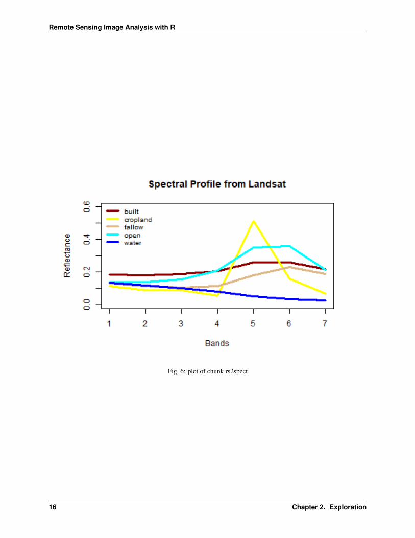
2.9 Spectral profiles

A plot of the spectrum (all bands) for pixels representing a certain earth surface features (e.g. water) is known asa spectral profile. Such profiles demonstrate the differences in spectral properties of various earth surface featuresand constitute the basis for image analysis. Spectral values can be extracted from any multispectral data set usingextract function. In the above example, we extracted values of Landsat data for the samples. These samplesinclude: cropland, water, fallow, built and open. First we compute the mean reflectance values for each class and eachband.

ms <- aggregate(df, list(ptsamp$class), mean)

# instead of the first column, we use rownamesrownames(ms) <- ms[,1]ms <- ms[,-1]ms## ultra.blue blue green red NIR SWIR1## built 0.1859386 0.18108087 0.18766994 0.20495042 0.25946109 0.26068728## cropland 0.1126274 0.09044816 0.08680185 0.05373526 0.51278337 0.15893917## fallow 0.1307048 0.11533900 0.10350018 0.11478698 0.18146030 0.22936763## open 0.1389726 0.13796324 0.15347092 0.20827845 0.34924460 0.36056706## water 0.1343485 0.11734908 0.10002031 0.07955140 0.05034531 0.03479516





## SWIR2## built 0.21610628## cropland 0.06836314## fallow 0.18799975## open 0.21426980## water 0.02827112

Now we will plot the mean spectra of these features.

# Create a vector of color for the land cover classes for use in plottingmycolor <- c('darkred', 'yellow', 'burlywood', 'cyan', 'blue')

#transform ms from a data.frame to a matrixms <- as.matrix(ms)

# First create an empty plotplot(0, ylim=c(0,0.6), xlim = c(1,7), type='n', xlab="Bands", ylab = "Reflectance")

# add the different classesfor (i in 1:nrow(ms)){lines(ms[i,], type = "l", lwd = 3, lty = 1, col = mycolor[i])

}

# Titletitle(main="Spectral Profile from Landsat", font.main = 2)

# Legendlegend("topleft", rownames(ms),

cex=0.8, col=mycolor, lty = 1, lwd =3, bty = "n")

The spectral profile shows (dis)similarity in the reflectance of different features on the earth’s surface (or above it).Unsurprisingly, the spectral signatures of ‘crop’ and ‘vegetation’ are similar. ‘Water’ shows relatively low reflectionin all wavelengths, and ‘built’, ‘fallow’ and ‘open’ have relatively high reflectance in the longer wavelengts.

2.9. Spectral profiles 15


Fig. 6: plot of chunk rs2spect


CHAPTER

THREE

BASIC MATHEMATICAL OPERATIONS

The raster package supports many mathematical operations. Math operations are generally performed per pixel.First we will learn about basic arithmetic operations on bands. First example is a custom math function that calculatesthe Normalized Difference Vegetation Index (NDVI). Learn more about vegetation indices here and NDVI.

We will use the same Landsat data as in Chapter 2.

library(raster)raslist <- paste0('data/rs/LC08_044034_20170614_B', 1:11, ".tif")landsat <- stack(raslist)landsatRGB <- landsat[[c(4,3,2)]]landsatFCC <- landsat[[c(5,4,3)]]

3.1 Vegetation indices

Let’s define a general function for a ratio based (vegetation) index. In the function below, img is a mutilayer Raster*object and i and k are the indices of the layers to compute the vegetation index.

VI <- function(img, k, i) {bk <- img[[k]]bi <- img[[i]]vi <- (bk - bi) / (bk + bi)return(vi)

}

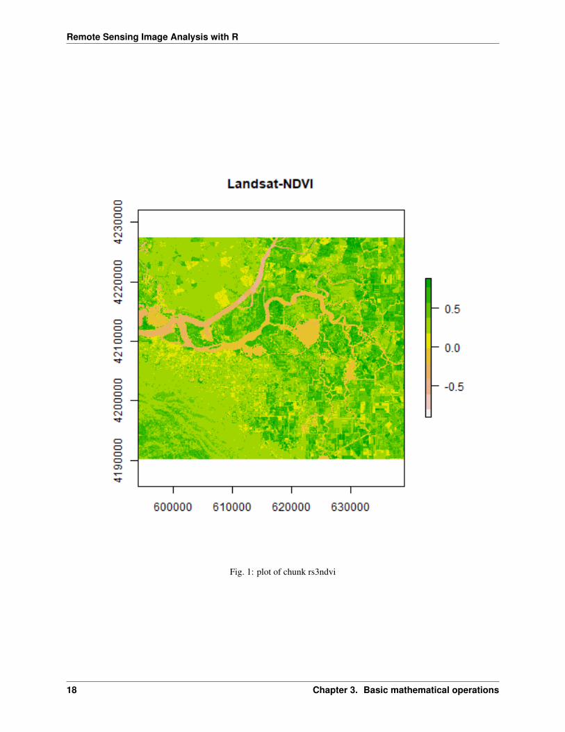
# For Landsat NIR = 5, red = 4.ndvi <- VI(landsat, 5, 4)plot(ndvi, col = rev(terrain.colors(10)), main = 'Landsat-NDVI')

You can see the variation in greenness from the plot.

Exercise 1 Adapt the function to compute indices which will highlight i) water and ii) built-up. Hint: Use the spectralprofile plot to find the bands having maximum and minimum reflectance for these two classes.

3.2 Histogram

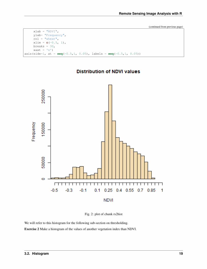
We can explore the distribution of values contained within our raster using the hist() function which produces ahistogram. Histograms are often useful in identifying outliers and bad data values in our raster data.

# view histogram of datahist(ndvi,

main = "Distribution of NDVI values",


17

http://www.un-spider.org/links-and-resources/data-sources/daotm/daotm-vegetation

http://phenology.cr.usgs.gov/ndvi_foundation.php


Fig. 1: plot of chunk rs3ndvi

18 Chapter 3. Basic mathematical operations



xlab = "NDVI",ylab= "Frequency",col = "wheat",xlim = c(-0.5, 1),breaks = 30,xaxt = 'n')

axis(side=1, at = seq(-0.5,1, 0.05), labels = seq(-0.5,1, 0.05))

Fig. 2: plot of chunk rs2hist

We will refer to this histogram for the following sub-section on thresholding.

Exercise 2 Make a histogram of the values of another vegetation index than NDVI.

3.2. Histogram 19


3.3 Thresholding

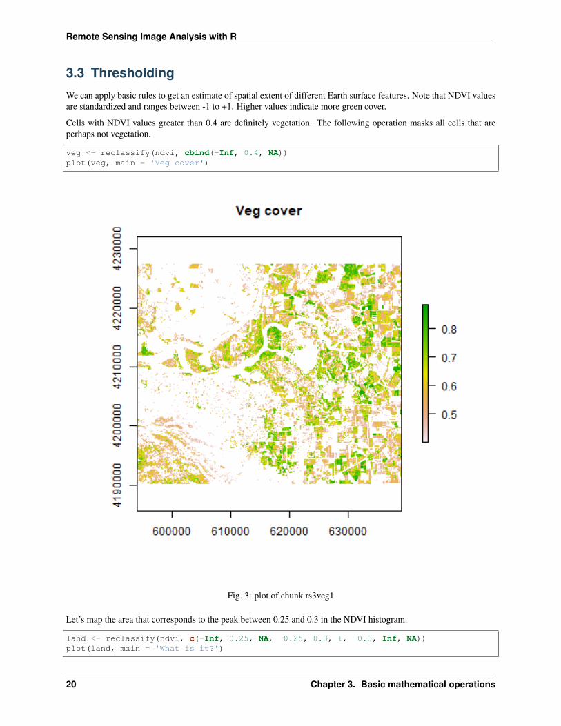
We can apply basic rules to get an estimate of spatial extent of different Earth surface features. Note that NDVI valuesare standardized and ranges between -1 to +1. Higher values indicate more green cover.

Cells with NDVI values greater than 0.4 are definitely vegetation. The following operation masks all cells that areperhaps not vegetation.

veg <- reclassify(ndvi, cbind(-Inf, 0.4, NA))plot(veg, main = 'Veg cover')

Fig. 3: plot of chunk rs3veg1

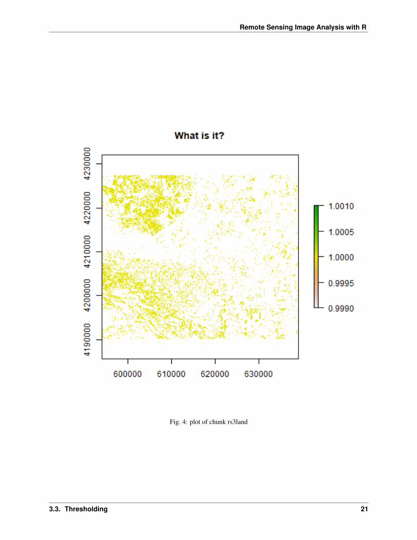
Let’s map the area that corresponds to the peak between 0.25 and 0.3 in the NDVI histogram.

land <- reclassify(ndvi, c(-Inf, 0.25, NA, 0.25, 0.3, 1, 0.3, Inf, NA))plot(land, main = 'What is it?')



Fig. 4: plot of chunk rs3land

3.3. Thresholding 21


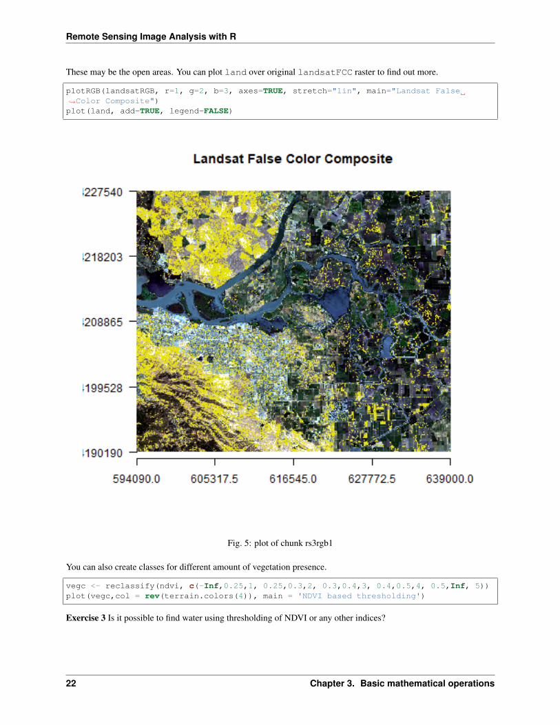
These may be the open areas. You can plot land over original landsatFCC raster to find out more.

plotRGB(landsatRGB, r=1, g=2, b=3, axes=TRUE, stretch="lin", main="Landsat False→˓Color Composite")plot(land, add=TRUE, legend=FALSE)

Fig. 5: plot of chunk rs3rgb1

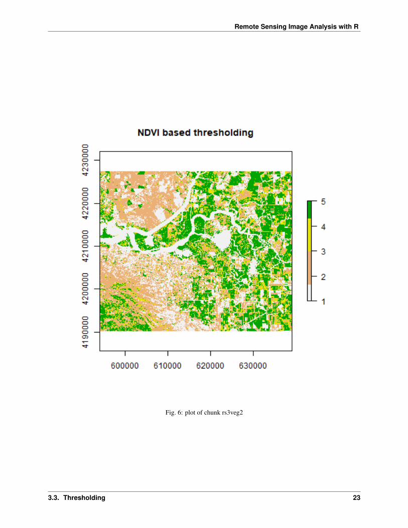
You can also create classes for different amount of vegetation presence.

vegc <- reclassify(ndvi, c(-Inf,0.25,1, 0.25,0.3,2, 0.3,0.4,3, 0.4,0.5,4, 0.5,Inf, 5))plot(vegc,col = rev(terrain.colors(4)), main = 'NDVI based thresholding')

Exercise 3 Is it possible to find water using thresholding of NDVI or any other indices?



Fig. 6: plot of chunk rs3veg2

3.3. Thresholding 23


3.4 Principal component analysis

Multi-spectral data are sometimes transformed to helps to reduce the dimensioanlity and noise in the data. The princi-pal components transform is a generic data reduction method that can be used to create a few uncorrelated bands froma larger set of correlated bands.

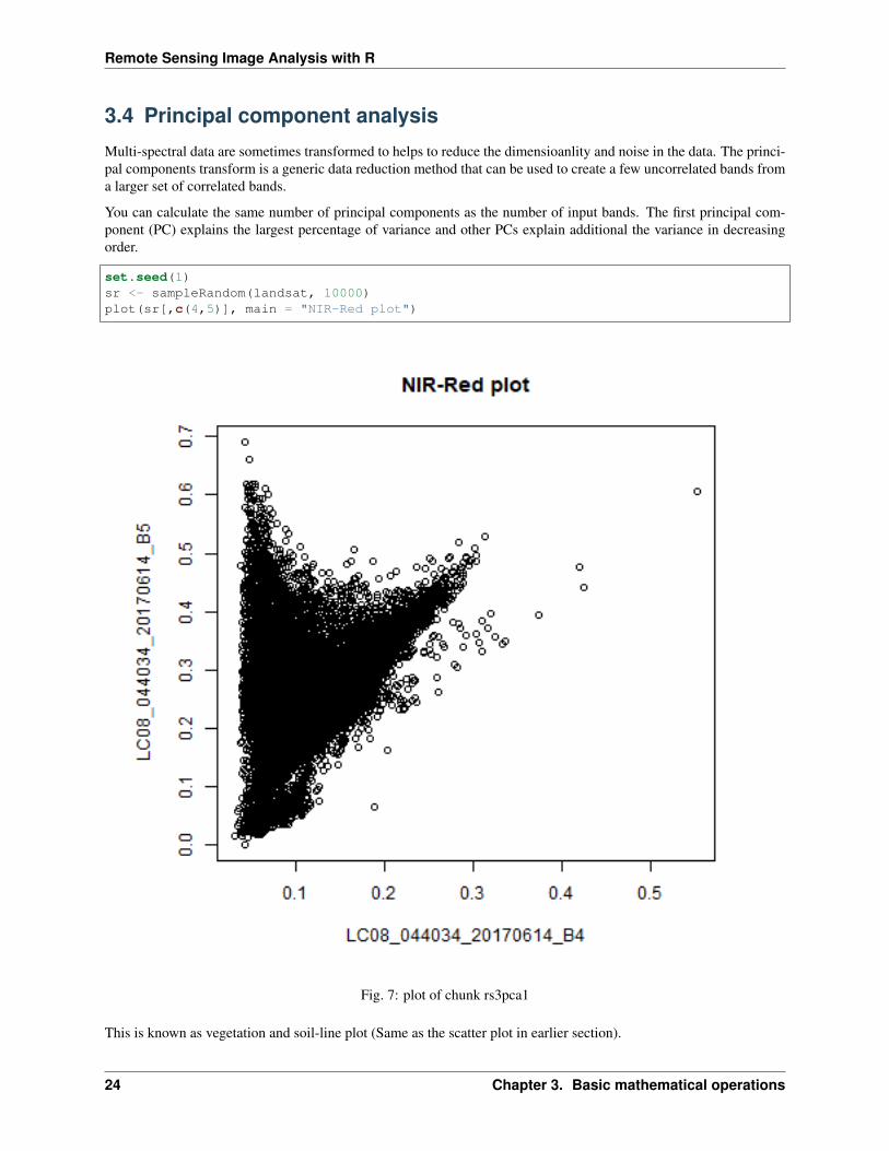
You can calculate the same number of principal components as the number of input bands. The first principal com-ponent (PC) explains the largest percentage of variance and other PCs explain additional the variance in decreasingorder.

set.seed(1)sr <- sampleRandom(landsat, 10000)plot(sr[,c(4,5)], main = "NIR-Red plot")

Fig. 7: plot of chunk rs3pca1

This is known as vegetation and soil-line plot (Same as the scatter plot in earlier section).



Exercise 4 Can you guess the directions of ‘principal components’ from this scatter plot?

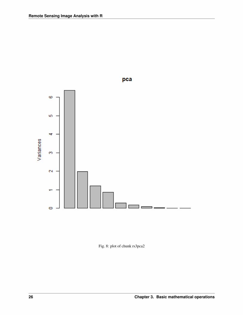
pca <- prcomp(sr, scale = TRUE)pca## Standard deviations (1, .., p=11):## [1] 2.52687022 1.40533428 1.09901821 0.92507423 0.53731672 0.42657919## [7] 0.28002273 0.12466139 0.09031384 0.04761419 0.03609857#### Rotation (n x k) = (11 x 11):## PC1 PC2 PC3 PC4## LC08_044034_20170614_B1 0.2973469 -0.3516438 -0.29454767 -0.06983456## LC08_044034_20170614_B2 0.3387629 -0.3301194 -0.16407835 -0.03803678## LC08_044034_20170614_B3 0.3621173 -0.2641152 0.07373240 0.04090884## LC08_044034_20170614_B4 0.3684797 -0.1659582 0.10260552 0.03680852## LC08_044034_20170614_B5 0.1546322 0.1816252 0.71354112 0.32017620## LC08_044034_20170614_B6 0.3480230 0.2108982 0.23064060 0.16598851## LC08_044034_20170614_B7 0.3496281 0.2384417 -0.11662258 0.07600209## LC08_044034_20170614_B8 0.3490464 -0.2007305 0.08765521 0.02303421## LC08_044034_20170614_B9 0.1314827 0.1047365 0.33741447 -0.92325315## LC08_044034_20170614_B10 0.2497611 0.4912132 -0.29286315 -0.02950655## LC08_044034_20170614_B11 0.2472765 0.4931489 -0.29515754 -0.03176549## PC5 PC6 PC7 PC8## LC08_044034_20170614_B1 0.49474685 0.175510232 -0.23948553 0.215745065## LC08_044034_20170614_B2 0.22121122 0.094184121 0.06447037 0.216537517## LC08_044034_20170614_B3 0.08482031 0.009040232 0.30511210 -0.518233675## LC08_044034_20170614_B4 -0.33835490 -0.066844529 0.60174786 0.012437959## LC08_044034_20170614_B5 0.51960822 -0.059561476 -0.07348455 -0.083217504## LC08_044034_20170614_B6 -0.29437062 0.317984598 -0.02106132 0.632178645## LC08_044034_20170614_B7 -0.25404931 0.525411720 -0.40543545 -0.478543437## LC08_044034_20170614_B8 -0.31407992 -0.673584139 -0.52642131 0.003527306## LC08_044034_20170614_B9 0.03040161 0.059642905 -0.03152221 -0.002775800## LC08_044034_20170614_B10 0.16317572 -0.243735973 0.14341520 0.041736319## LC08_044034_20170614_B11 0.19294569 -0.241611777 0.11997475 -0.022446494## PC9 PC10 PC11## LC08_044034_20170614_B1 0.122812108 0.535959306 0.1203473847## LC08_044034_20170614_B2 0.091063964 -0.773112627 -0.1817872036## LC08_044034_20170614_B3 -0.644305383 0.070860458 0.0540175730## LC08_044034_20170614_B4 0.543822097 0.218324141 0.0135097158## LC08_044034_20170614_B5 0.209682702 -0.040186292 -0.0004965182## LC08_044034_20170614_B6 -0.397210135 0.089423617 -0.0045305608## LC08_044034_20170614_B7 0.248871690 -0.074907393 0.0003958921## LC08_044034_20170614_B8 -0.012642132 0.002411975 0.0007749022## LC08_044034_20170614_B9 0.003176077 -0.000832654 0.0019986985## LC08_044034_20170614_B10 -0.003574004 -0.158727672 0.6900281980## LC08_044034_20170614_B11 -0.043475408 0.148102091 -0.6878990264screeplot(pca)

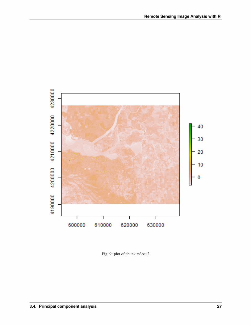
pci <- predict(landsat, pca, index = 1:2)plot(pci[[1]])

The first principal component highlights the boundaries between land use classes or spatial details, which is the mostcommon information among all wavelengths. it is difficult to understand what the second principal component ishighlighting. Lets try thresholding again:

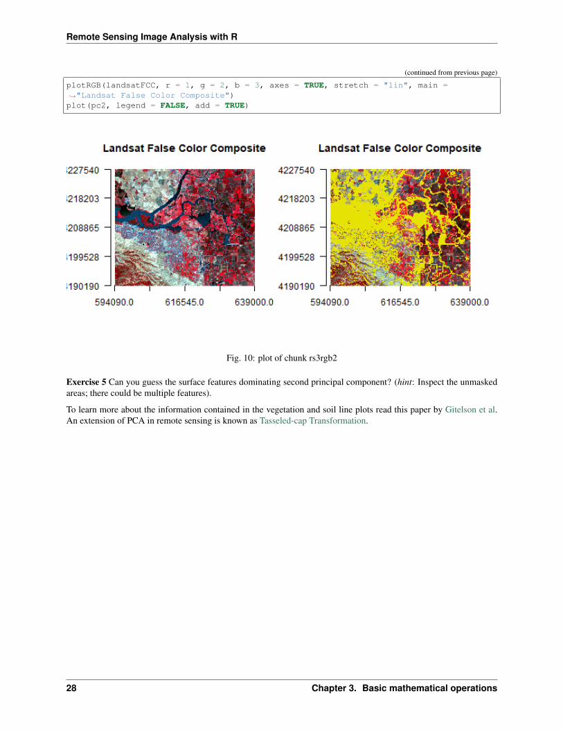
pc2 <- reclassify(pci[[2]], c(-Inf,0,1,0,Inf,NA))par(mfrow = c(1,2))plotRGB(landsatFCC, r = 1, g = 2, b = 3, axes = TRUE, stretch = "lin", main =→˓"Landsat False Color Composite")


3.4. Principal component analysis 25






3.4. Principal component analysis 27



plotRGB(landsatFCC, r = 1, g = 2, b = 3, axes = TRUE, stretch = "lin", main =→˓"Landsat False Color Composite")plot(pc2, legend = FALSE, add = TRUE)

Fig. 10: plot of chunk rs3rgb2

Exercise 5 Can you guess the surface features dominating second principal component? (hint: Inspect the unmaskedareas; there could be multiple features).

To learn more about the information contained in the vegetation and soil line plots read this paper by Gitelson et al.An extension of PCA in remote sensing is known as Tasseled-cap Transformation.


http://www.tandfonline.com/doi/abs/10.1080/01431160110107806#.V6hp_LgrKhd

http://wiki.landscapetoolbox.org/doku.php/remote_sensing_methods:tasseled-cap_transformation

CHAPTER

FOUR

UNSUPERVISED IMAGE CLASSIFICATION

In this chapter we explore unsupervised classification. Various unsupervised classification algorithms exist, and thechoice of algorithm can affect the results. We will explore only one algorithm (k-means) to illustrate the generalprinciple.

For this example, we will follow the National Land Cover Database 2011 (NLCD 2011) classification scheme for asubset of the Central Valley regions. You will use cloud-free composite image from Landsat 5 with 6 bands.

library(raster)## Loading required package: splandsat5 <- stack('data/rs/centralvalley-2011LT5.tif')names(landsat5) <- c('blue', 'green', 'red', 'NIR', 'SWIR1', 'SWIR2')

Exercise 1 Make a 3-band False Color Composite plot of landsat5.

In unsupervised classification, we don’t supply any training data. This particularly is useful when we don’t haveprior knowledge of the study area. The algorithm groups pixels with similar spectral characteristics into uniqueclusters/classes/groups following some statistically determined conditions (e.g. minimizing mean square root errorwithin each cluster). You have to re-label and combine these spectral clusters into information classes (for e.g. land-use land-cover). Unsupervised algorithms are often referred as clustering.

To get satisfactory results from unsupervised classification, a good practice is to start with large number of centers(more clusters) and merge/group/recode similar clusters by inspecting the original imagery.

Learn more about K-means and other unsupervised-supervised algorithms here.

We will perform unsupervised classification on a spatial subset of the ndvi layer.

ndvi <- (landsat5[['NIR']]-landsat5[['red']])/(landsat5[['NIR']]+landsat5[['red']])

We will do kmeans clustering of the ndvi data. First we use crop to make a spatial subset of the ndvi, to allowfor faster processing (you can select any extent using the drawExtent() function).

4.1 kmeans classification

# Extent to crop ndvi layere <- extent(-121.807, -121.725, 38.004, 38.072)

# crop landsat by the extentndvi <- crop(ndvi, e)ndvi## class : RasterLayer## dimensions : 252, 304, 76608 (nrow, ncol, ncell)## resolution : 0.0002694946, 0.0002694946 (x, y)


29

https://www.mrlc.gov/nlcd2011.php


http://nptel.ac.in/courses/105108077/module5/lecture19.pdf



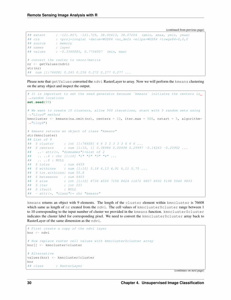
## extent : -121.807, -121.725, 38.00413, 38.07204 (xmin, xmax, ymin, ymax)## crs : +proj=longlat +datum=WGS84 +no_defs +ellps=WGS84 +towgs84=0,0,0## source : memory## names : layer## values : -0.3360085, 0.7756007 (min, max)

# convert the raster to vecor/matrixnr <- getValues(ndvi)str(nr)## num [1:76608] 0.245 0.236 0.272 0.277 0.277 ...

Please note that getValues converted the ndvi RasterLayer to array. Now we will perform the kmeans clusteringon the array object and inspect the output.

# It is important to set the seed generator because `kmeans` initiates the centers in→˓random locationsset.seed(99)

# We want to create 10 clusters, allow 500 iterations, start with 5 random sets using→˓"Lloyd" methodkmncluster <- kmeans(na.omit(nr), centers = 10, iter.max = 500, nstart = 5, algorithm=→˓"Lloyd")

# kmeans returns an object of class "kmeans"str(kmncluster)## List of 9## $ cluster : int [1:76608] 6 6 3 3 3 3 3 6 6 6 ...## $ centers : num [1:10, 1] 0.38986 0.00498 0.29997 -0.14263 -0.20902 ...## ..- attr(*, "dimnames")=List of 2## .. ..$ : chr [1:10] "1" "2" "3" "4" ...## .. ..$ : NULL## $ totss : num 6459## $ withinss : num [1:10] 5.18 6.13 4.91 6.11 5.75 ...## $ tot.withinss: num 55.8## $ betweenss : num 6403## $ size : int [1:10] 8736 4550 7156 8624 11672 6807 8932 5198 5040 9893## $ iter : int 221## $ ifault : NULL## - attr(*, "class")= chr "kmeans"

kmeans returns an object with 9 elements. The length of the cluster element within kmncluster is 76608which same as length of nr created from the ndvi. The cell values of kmncluster$cluster range between 1to 10 corresponding to the input number of cluster we provided in the kmeans function. kmncluster$clusterindicates the cluster label for corresponding pixel. We need to convert the kmncluster$cluster array back toRasterLayer of the same dimension as the ndvi.

# First create a copy of the ndvi layerknr <- ndvi

# Now replace raster cell values with kmncluster$cluster arrayknr[] <- kmncluster$cluster

# Alternativevalues(knr) <- kmncluster$clusterknr## class : RasterLayer


30 Chapter 4. Unsupervised Image Classification



## dimensions : 252, 304, 76608 (nrow, ncol, ncell)## resolution : 0.0002694946, 0.0002694946 (x, y)## extent : -121.807, -121.725, 38.00413, 38.07204 (xmin, xmax, ymin, ymax)## crs : +proj=longlat +datum=WGS84 +no_defs +ellps=WGS84 +towgs84=0,0,0## source : memory## names : layer## values : 1, 10 (min, max)

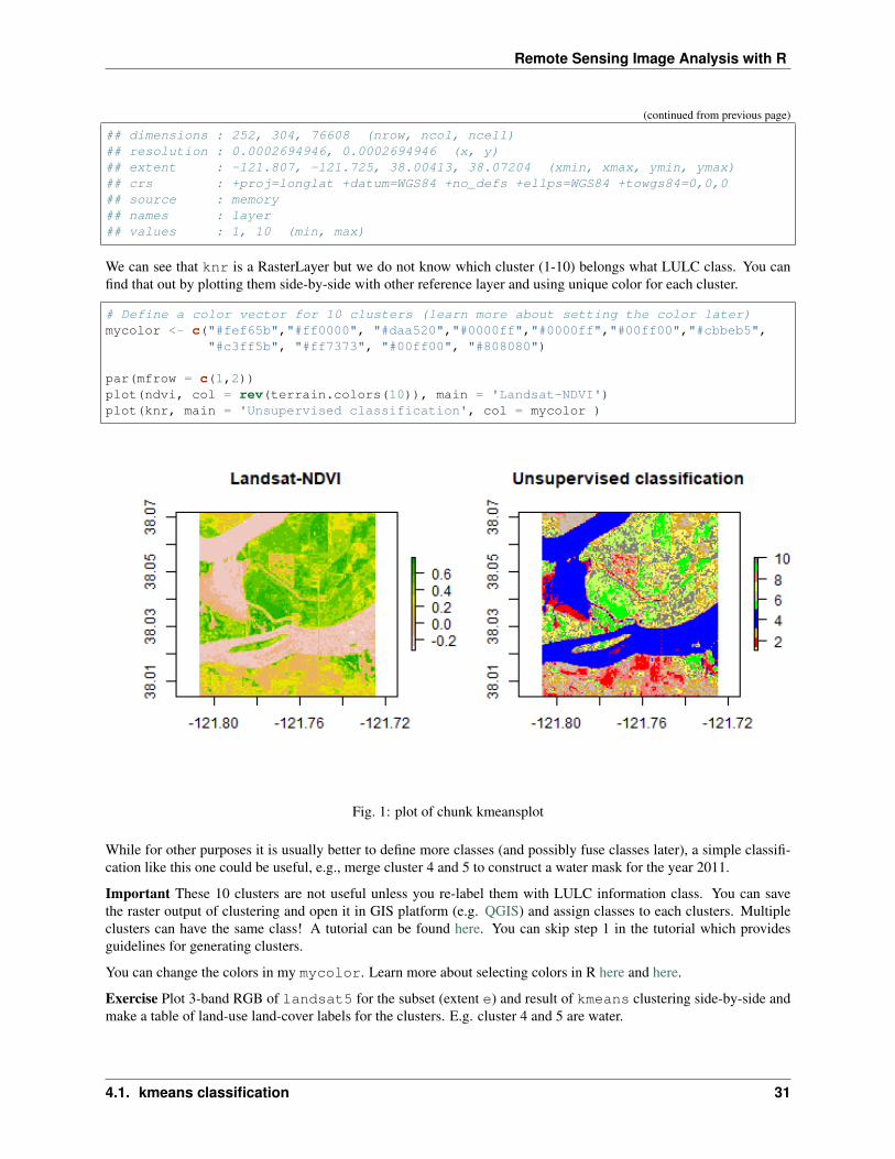
We can see that knr is a RasterLayer but we do not know which cluster (1-10) belongs what LULC class. You canfind that out by plotting them side-by-side with other reference layer and using unique color for each cluster.

# Define a color vector for 10 clusters (learn more about setting the color later)mycolor <- c("#fef65b","#ff0000", "#daa520","#0000ff","#0000ff","#00ff00","#cbbeb5",

"#c3ff5b", "#ff7373", "#00ff00", "#808080")

par(mfrow = c(1,2))plot(ndvi, col = rev(terrain.colors(10)), main = 'Landsat-NDVI')plot(knr, main = 'Unsupervised classification', col = mycolor )

Fig. 1: plot of chunk kmeansplot

While for other purposes it is usually better to define more classes (and possibly fuse classes later), a simple classifi-cation like this one could be useful, e.g., merge cluster 4 and 5 to construct a water mask for the year 2011.

Important These 10 clusters are not useful unless you re-label them with LULC information class. You can savethe raster output of clustering and open it in GIS platform (e.g. QGIS) and assign classes to each clusters. Multipleclusters can have the same class! A tutorial can be found here. You can skip step 1 in the tutorial which providesguidelines for generating clusters.

You can change the colors in my mycolor. Learn more about selecting colors in R here and here.

Exercise Plot 3-band RGB of landsat5 for the subset (extent e) and result of kmeans clustering side-by-side andmake a table of land-use land-cover labels for the clusters. E.g. cluster 4 and 5 are water.

4.1. kmeans classification 31

https://qgis.org/en/site/about/index.html

http://wiki.awf.forst.uni-goettingen.de/wiki/index.php/Unsupervised_classification_(Tutorial)

http://www.melissaclarkson.com/resources/R_guides/documents/colors_Ver2.pdf

https://www.nceas.ucsb.edu/~frazier/RSpatialGuides/colorPaletteCheatsheet.pdf


32 Chapter 4. Unsupervised Image Classification

CHAPTER

FIVE

SUPERVISED IMAGE CLASSIFICATION

Here we explore supervised classification. Various supervised classification algorithms exist, and the choice of algo-rithm can affect the results. Here we explore two related algorithms (CART and RandomForest).

In supervised classification, we have prior knowledge about some of the land-cover types through, for example, field-work, reference spatial data or interpretation of high resolution imagery (such as available on Google maps). Specificsites in the study area that represent homogeneous examples of these known land-cover types are identified. Theseareas are commonly referred to as training sites because the spectral properties of these sites are used to train theclassification algorithm.

The following examples uses a Classification and Regression Trees (CART) classifier (Breiman et al. 1984) (furtherreading to predict land use land cover classes in the study area.

We will perform the following steps:

• Generate sample sites based on a reference raster

• Extract cell values from Landsat data for the sample sites

• Train the classifier using training samples

• Classify the Landsat data using the trained model

• Evaluate the accuracy of the model

5.1 Reference data

The National Land Cover Database 2011 (NLCD 2011) is a land cover product for the USA. NLCD is a 30-m Landsat-based land cover database spanning 4 epochs (1992, 2001, 2006 and 2011). NLCD 2011 is based primarily on adecision-tree classification of circa 2011 Landsat data.

You can find the class names in NCLD 2011 (here)[https://www.mrlc.gov/nlcd11_leg.php]. It has two pairs of class-values and classnames that correspond to the levels of land use and land cover classification system. These levelsusually represent the level of complexity, level I being the simplest with broad land use land cover categories. Readthis report by Anderson et al to learn more about this land use and land cover classification system for use with RemoteSensor data.

library(raster)nlcd <- brick('data/rs/nlcd-L1.tif')names(nlcd) <- c("nlcd2001", "nlcd2011")

# The class names and colors for plottingnlcdclass <- c("Water", "Developed", "Barren", "Forest", "Shrubland", "Herbaceous",→˓"Planted/Cultivated", "Wetlands")classdf <- data.frame(classvalue1 = c(1,2,3,4,5,7,8,9), classnames1 = nlcdclass)


33

https://doi.org/10.1016/S0034-4257(97)00049-7

https://doi.org/10.1016/S0034-4257(97)00049-7


https://www.mrlc.gov/nlcd11_leg.php

https://pubs.usgs.gov/pp/0964/report.pdf



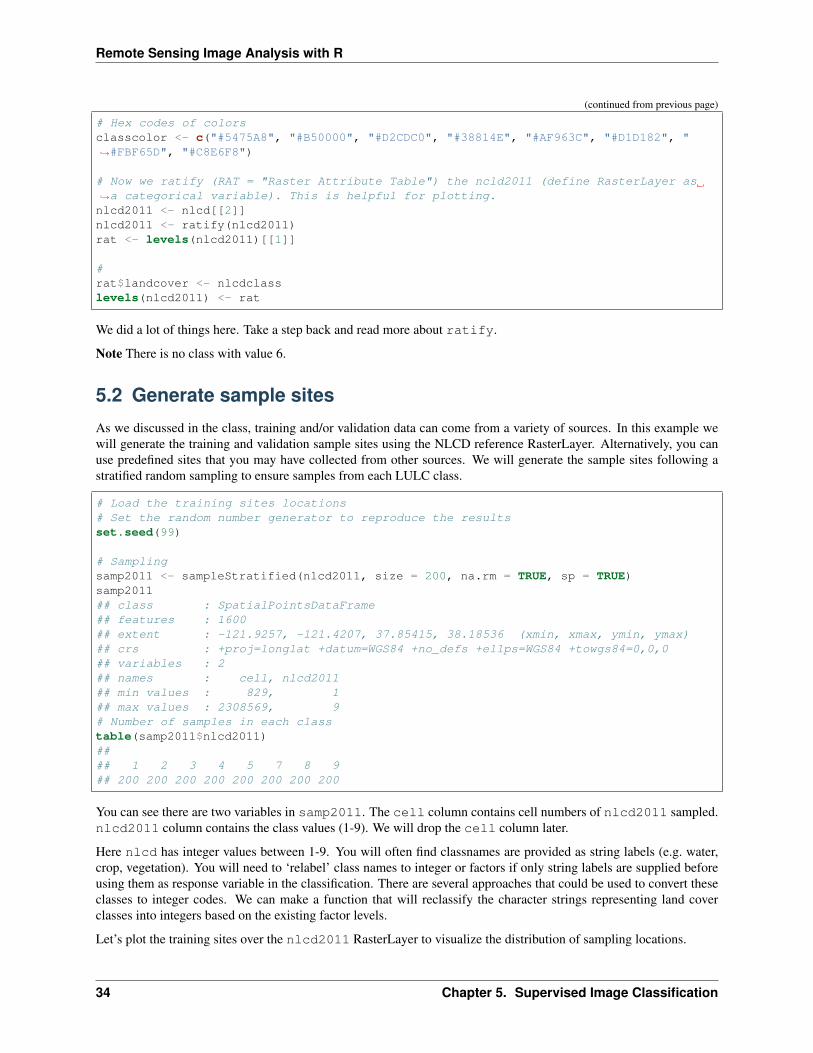
# Hex codes of colorsclasscolor <- c("#5475A8", "#B50000", "#D2CDC0", "#38814E", "#AF963C", "#D1D182", "→˓#FBF65D", "#C8E6F8")

# Now we ratify (RAT = "Raster Attribute Table") the ncld2011 (define RasterLayer as→˓a categorical variable). This is helpful for plotting.nlcd2011 <- nlcd[[2]]nlcd2011 <- ratify(nlcd2011)rat <- levels(nlcd2011)[[1]]

#rat$landcover <- nlcdclasslevels(nlcd2011) <- rat

We did a lot of things here. Take a step back and read more about ratify.

Note There is no class with value 6.

5.2 Generate sample sites

As we discussed in the class, training and/or validation data can come from a variety of sources. In this example wewill generate the training and validation sample sites using the NLCD reference RasterLayer. Alternatively, you canuse predefined sites that you may have collected from other sources. We will generate the sample sites following astratified random sampling to ensure samples from each LULC class.

# Load the training sites locations# Set the random number generator to reproduce the resultsset.seed(99)

# Samplingsamp2011 <- sampleStratified(nlcd2011, size = 200, na.rm = TRUE, sp = TRUE)samp2011## class : SpatialPointsDataFrame## features : 1600## extent : -121.9257, -121.4207, 37.85415, 38.18536 (xmin, xmax, ymin, ymax)## crs : +proj=longlat +datum=WGS84 +no_defs +ellps=WGS84 +towgs84=0,0,0## variables : 2## names : cell, nlcd2011## min values : 829, 1## max values : 2308569, 9# Number of samples in each classtable(samp2011$nlcd2011)#### 1 2 3 4 5 7 8 9## 200 200 200 200 200 200 200 200

You can see there are two variables in samp2011. The cell column contains cell numbers of nlcd2011 sampled.nlcd2011 column contains the class values (1-9). We will drop the cell column later.

Here nlcd has integer values between 1-9. You will often find classnames are provided as string labels (e.g. water,crop, vegetation). You will need to ‘relabel’ class names to integer or factors if only string labels are supplied beforeusing them as response variable in the classification. There are several approaches that could be used to convert theseclasses to integer codes. We can make a function that will reclassify the character strings representing land coverclasses into integers based on the existing factor levels.

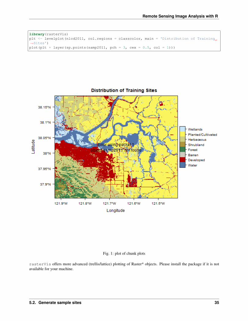
Let’s plot the training sites over the nlcd2011 RasterLayer to visualize the distribution of sampling locations.

34 Chapter 5. Supervised Image Classification


library(rasterVis)plt <- levelplot(nlcd2011, col.regions = classcolor, main = 'Distribution of Training→˓Sites')plot(plt + layer(sp.points(samp2011, pch = 3, cex = 0.5, col = 1)))

Fig. 1: plot of chunk plots

rasterVis offers more advanced (trellis/lattice) plotting of Raster* objects. Please install the package if it is notavailable for your machine.

5.2. Generate sample sites 35


5.3 Extract cell values for the sample sites

landsat5 <- stack('data/rs/centralvalley-2011LT5.tif')names(landsat5) <- c('blue', 'green', 'red', 'NIR', 'SWIR1', 'SWIR2')

Once we have the sites, we can extract the cell values from landsat5 RasterStack. These band values will be thepredictor variables and “classvalues” from nlcd2011 will be the response variable.

# Extract the layer values for the locationssampvals <- extract(landsat5, samp2011, df = TRUE)

# sampvals no longer has the spatial information. To keep the spatial information you→˓use `sp = TRUE` argument in `extract` function.

# drop the ID columnsampvals <- sampvals[, -1]

# combine the class information with extracted valuessampdata <- data.frame(classvalue = samp2011@data$nlcd2011, sampvals)

5.4 Train the classifier using training samples

Now we will train the classification algorithm using training2011 dataset.

library(rpart)

# Train the modelcart <- rpart(as.factor(classvalue)~., data=sampdata, method = 'class', minsplit = 5)

# print(model.class)

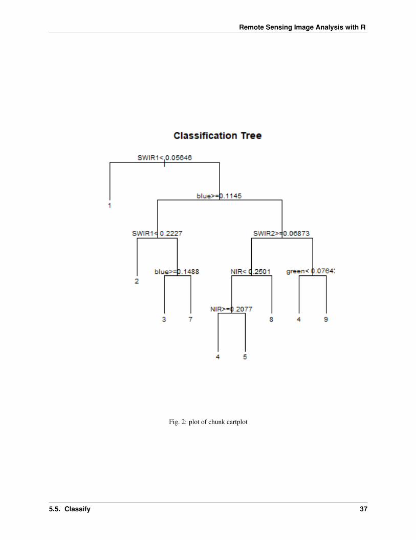
# Much cleaner way is to plot the trained classification treeplot(cart, uniform=TRUE, main="Classification Tree")text(cart, cex = 0.8)

In the classification tree plot classvalues are printed at the leaf node. You can find the corresponding land use landcover names from the classdf dataframe.

See ?rpart.control to set different parameters for building the model.

You can print/plot more about the cart model created in the previous example. E.g. you can use plotcp(cart)to learn about the cost-complexity (cp argument in rpart).

5.5 Classify

Now we have our trained classification model (cart), we can use it to make predictions, that is, to classify all cells inthe landsat5 RasterStack.

Important The names in the Raster object to be classified should exactly match those expected by the model. Thiswill be the case if the same Raster object was used (via extract) to obtain the values to fit the model (previous example).

# Now predict the subset data based on the model; prediction for entire area takes→˓longer timepr2011 <- predict(landsat5, cart, type='class')pr2011




Fig. 2: plot of chunk cartplot

5.5. Classify 37



## class : RasterLayer## dimensions : 1230, 1877, 2308710 (nrow, ncol, ncell)## resolution : 0.0002694946, 0.0002694946 (x, y)## extent : -121.9258, -121.42, 37.85402, 38.1855 (xmin, xmax, ymin, ymax)## crs : +proj=longlat +datum=WGS84 +no_defs +ellps=WGS84 +towgs84=0,0,0## source : memory## names : layer## values : 1, 9 (min, max)## attributes :## ID value## from: 1 1## to : 8 9

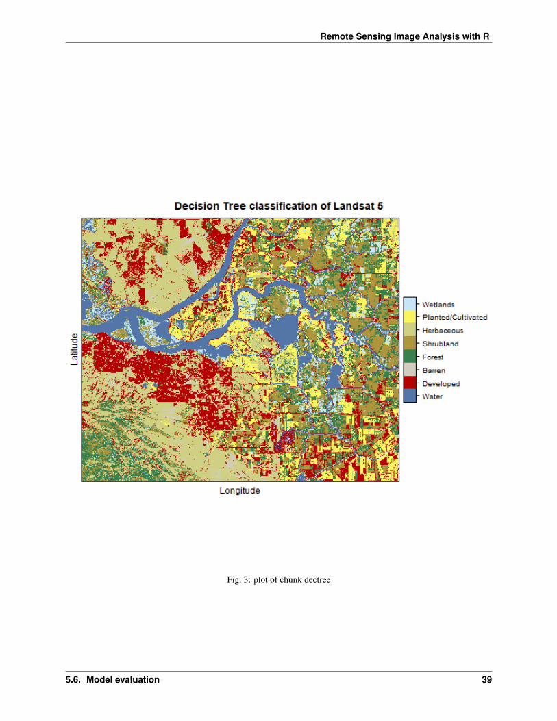
Now plot the classification result using rasetrVis. See will set the classnames for the classvalues.

pr2011 <- ratify(pr2011)

rat <- levels(pr2011)[[1]]

rat$legend <- classdf$classnames

levels(pr2011) <- rat

levelplot(pr2011, maxpixels = 1e6,col.regions = classcolor,scales=list(draw=FALSE),main = "Decision Tree classification of Landsat 5")

Exercise 1 Plot nlcd2011 and pr2011 side-by-side and comment about the accuracy of the prediction (e.g. mixingbetween cultivated crops, pasture, grassland and shrubs).

You may need to select more samples and use additional predictor variables. The choice of classifier also plays animportant role.

5.6 Model evaluation

Now let’s assess the accuracy of the model to get an idea of how accurate the classified map might be. Two widely usedmeasures in remote sensing community are “overall accuracy” and “kappa”. You can perform the accuracy assessmentusing the independent samples (validation2011).

To evaluate any model, you can use k-fold cross-validation. In this technique the data used to fit the model is split intok groups (typically 5 groups). In turn, one of the groups will be used for model testing, while the rest of the data isused for model training (fitting).

library(dismo)set.seed(99)j <- kfold(sampdata, k = 5, by=sampdata$classvalue)table(j)## j## 1 2 3 4 5## 320 320 320 320 320

Now we train and test the model five times, each time computing a confusion matrix that we store in a list.

x <- list()




Fig. 3: plot of chunk dectree

5.6. Model evaluation 39



for (k in 1:5) {train <- sampdata[j!= k, ]test <- sampdata[j == k, ]cart <- rpart(as.factor(classvalue)~., data=train, method = 'class', minsplit = 5)pclass <- predict(cart, test, type='class')# create a data.frame using the reference and predictionx[[k]] <- cbind(test$classvalue, as.integer(pclass))

}

Now combine the five list elements into a single data.frame, using do.call and compute a confusion matrix.

y <- do.call(rbind, x)y <- data.frame(y)colnames(y) <- c('observed', 'predicted')

conmat <- table(y)# change the name of the classescolnames(conmat) <- classdf$classnamesrownames(conmat) <- classdf$classnamesconmat## predicted## observed Water Developed Barren Forest Shrubland Herbaceous## Water 172 6 1 3 3 1## Developed 8 93 22 10 8 37## Barren 6 54 52 6 8 62## Forest 0 3 2 102 49 8## Shrubland 0 8 1 52 105 12## Herbaceous 1 16 24 4 16 121## Planted/Cultivated 2 20 5 24 37 24## Wetlands 14 12 1 32 25 16## predicted## observed Planted/Cultivated Wetlands## Water 1 13## Developed 20 2## Barren 5 7## Forest 13 23## Shrubland 17 5## Herbaceous 17 1## Planted/Cultivated 81 7## Wetlands 32 68

Exercise 2 Comment on the miss-classification between different classes.

Exercise 3 Can you think of ways to to improve the accuracy.

Compute overall accuracy and Kappa statistics.

Overall accuray

# number of casesn <- sum(conmat)n## [1] 1600

# number of correctly classified cases per classdiag <- diag(conmat)





# Overall AccuracyOA <- sum(diag) / nOA## [1] 0.49625

Kappa

# observed (true) cases per classrowsums <- apply(conmat, 1, sum)p <- rowsums / n

# predicted cases per classcolsums <- apply(conmat, 2, sum)q <- colsums / n

expAccuracy <- sum(p*q)kappa <- (OA - expAccuracy) / (1 - expAccuracy)kappa## [1] 0.4242857

Producer and user accuracy

# Producer accuracyPA <- diag / colsums

# User accuracyUA <- diag / rowsums

outAcc <- data.frame(producerAccuracy = PA, userAccuracy = UA)

outAcc## producerAccuracy userAccuracy## Water 0.8472906 0.860## Developed 0.4386792 0.465## Barren 0.4814815 0.260## Forest 0.4377682 0.510## Shrubland 0.4183267 0.525## Herbaceous 0.4306050 0.605## Planted/Cultivated 0.4354839 0.405## Wetlands 0.5396825 0.340

Exercise 4 Perform the classification using Random Forest classifiers from the package `randomForest <https://cran.r-project.org/web/packages/randomForest/index.html>‘__. For help see this discussion.

Exercise 5 Plot the results of rpart and ’rf‘ classifier side-by-side.

Exercise 6 (optional) Please repeat the steps for the year 2001 using rpart. You will use cloud-free compositeimage from Landsat 7 with 6-bands. The reference data will be the National Land Cover Database 2001 (NLCD 2001)for the subset of the Central Valley regions.

Exercise 7 (optional) You have been training your classifiers using 160 samples for each class. Now we want to seethe effect of sample size on classification. Please repeat the steps with different subset of the sample size (e.g. 120,100). Use the same holdout samples for accuracy assessment.

5.6. Model evaluation 41

https://cran.r-project.org/web/packages/randomForest/index.html

https://cran.r-project.org/web/packages/randomForest/index.html

https://gis.stackexchange.com/questions/39021/how-to-perform-random-forest-land-cover-classification



Documents

Remote Sensing Image Analysis with R · landsat