Remotesensing-04-00271_Environmental and Sensor Limitations in Optical Remote Sensing of Coral Reef

Remote Sens. 2012, 4, 271-302; doi:10.3390/rs4010271

Remote Sensing ISSN 2072-4292

www.mdpi.com/journal/remotesensing Article

Environmental and Sensor Limitations in Optical Remote Sensing of Coral Reefs: Implications for Monitoring and Sensor Design

John D. Hedley 1,2,*, Chris M. Roelfsema 3, Stuart R. Phinn 3 and Peter J. Mumby 1,4

1 School of Biosciences, University of Exeter, Prince of Wales Road, Exeter EX4 4PS, UK 2 ARGANS Ltd., Tamar Science Park, Derriford, Plymouth PL6 8BT, UK 3 Center for Spatial Environmental Research, School of Geography Planning and Environmental

Management, University of Queensland, Brisbane, QLD 4072, Australia;

E-Mails: [email protected] (C.M.R.); [email protected] (S.R.P.) 4 Marine Spatial Ecology Lab, School of Biological Sciences, University of Queensland, Brisbane,

QLD 4072, Australia; E-Mail: [email protected]

* Author to whom correspondence should be addressed; E-Mail: [email protected];

Tel.: +44-1752-764-298; Fax: +44-1752-772-227.

Received: 1 December 2011; in revised form: 9 January 2012 / Accepted: 9 January 2012 /

Published: 23 January 2012

Abstract: A generic method was developed for analysing the capabilities of optical remote

sensing of aquatic systems in terms of environmental components and imaging sensor

configurations. The method was based on a component based model of the entire system in

which not only benthic composition but other environmental components such as water

inherent optical properties (IOPs), bathymetry, sun elevation, wind speed and sensor noise

characteristics were defined by datasets with the potential to include across-image

variation. The model was applied to data from Pacific Ocean reefs in an airborne sensor

context to estimate the primary environmental or sensor factors confounding discrimination

of benthic mixtures of key reef types: live coral, bleached coral, dead coral and

macroalgae. Results indicate that spectral variation of benthic types and sub-pixel mixing is

the primary limiting factor for benthic mapping objectives, whereas instrument noise levels

are a minor factor.

Keywords: remote sensing; benthic; aquatic; inherent optical properties; coral reefs;

bleaching

OPEN ACCESS

Remote Sens. 2012, 4

272

1. Introduction

Analysis of satellite and airborne imagery has shown that remote sensing offers the potential to monitor

important ecological events on coral reefs, such as stress induced coral bleaching (loss of symbiotic

zooxanthellae [1], coral mortality and phase shifts to macroalgal dominance [2,3]. However, practical

image-based coral reef remote sensing research has, by necessity, been performed on a rather ad hoc

basis, producing a variety results that are sensor-specific, algorithm-specific and site-specific [3–5].

Clearly, application-based results are an inefficient method to estimate the maximum potential of coral

reef remote sensing in general terms, or to demonstrate how to realise that potential through analytical

algorithms and sensor design. Modelling studies are therefore required to evaluate the upper or lower

theoretical bounds of remote sensing capability and guide the design of appropriate sensors. Various

studies have assessed the spectral separability of reef benthic classes and in some cases advised on

optimal wavelengths for discrimination [6–10]. However, these studies have focused on variation in

benthic type in situ spectral reflectance and sensor noise as the primary sources of noise in the system.

In reality, within the spatial scale of a single remotely-sensed image, coral reef waters can exhibit a

wide range of water clarity from Case 1 oceanic-like fore-reef sites through shallow lagoonal sites

subject to wind and tidal driven re-suspension of sediments, to complex sediment and CDOM-loaded

terrestrial inputs [11,12]. Around spur and groove zones and on patch reefs depth can also vary with

vertical scales almost equal to the total height of the water column. The spectral signal for a given

benthic type is therefore subject to these additional variations within an image, and discrimination may

be consequently confounded. Put simply, two distinct benthic types at different depths (for example)

may be spectrally indistinguishable in a remotely sensed image.

Previous studies have shown that basic reef benthic types such as coral, macroalgae, seagrass and

sand are fundamentally separable by hyperspectral reflectance signatures [5,6,8,13]. Thus, modelling

water column radiative transfer without factoring-in any variation in clarity or depth leads to the

inevitable conclusion that, assuming optimal spectral bands, sensor signal-to-noise characteristics

(SNR) are the predominant limiting factor and that remote sensing capability is “sensor limited”, i.e.,

reflectance spectra at depth are increasingly similar but still technically separable by a sensor with a

high SNR (Figure 1). In reality, however, the system may be “environmentally limited” with sensor

SNR issues becoming insignificant compared to the variation in reflectance caused by variance in

water column depth and optical properties (Figure 1). Since these processes will also be a function of

wavelength, the number, position and width of the sensor spectral bands will also contribute to “sensor

limitation”. Sensor spatial resolution and the spatial heterogeneity of target features will also interact to

introduce sub-pixel spectral mixing and reduce the capability for benthic class discrimination.

Depending on perspective, this process could be considered either a sensor limitation or an

environmental limitation.


273

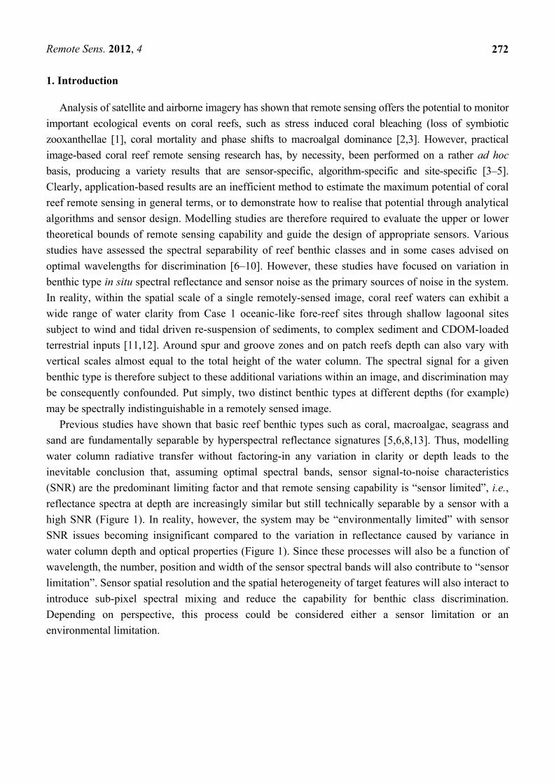
Figure 1. Sensor-limited vs. environmentally limited remote sensing. At each stage of the

remote sensing system the variation in classes to be discriminated is expressed by the

distribution of their member populations in spectral space, e.g., as illustrated in two bands

b1, b2. The extent of overlap between two classes expresses their fundamental

inseparability. Variation in different components of the system, such as benthic class

spectral variation, variance in water clarity, or sensor noise, contributes to overall variation

in the recorded signal. Sensor-limited objectives are those for which a change in sensor

design characteristics will improve separability despite environmental sources of variation.

A possible measure of class overlap is to attempt to insert a separating plane in spectral

space between A and B, linear discriminant analysis (LDA) is one method to achieve this.

Estimating benthic class separability of in situ spectra or at specific depths [6,9] is of little practical

relevance when in general, without ancillary data, the depth of individual pixels in a remotely sensed

image is unknown. Rather, the separability of classes as they appear across the expected range of

depths is more relevant (Figure 2). Put simply, there may be a problem where “coral” at one depth

looks like “algae” at a different depth, for example. In such cases neither depth nor benthic class can

be reliably determined from reflectance alone. An important concept developed in this study is that the


274

variance in spectral reflectance introduced by environmental factors and sensor characteristics is key to

understanding the fundamental limits of the separability of benthic classes. For example, if a model is

used to estimate the above-water reflectance resulting from two distinct in situ benthic reflectances, as

depth in increased the modelled reflectances will become increasingly similar. However the two

reflectances will continues to be numerically separable unless a factor is considered which will

introduce variance into the measured signal, e.g., sensor noise, or a small random variance in one of

the depths. The total achievable separability is therefore a complex result of the interaction of the

absolute effect and variance induced by the environmental and sensor components in the system,

framed by the structure of the question that is to be asked of the data (Figure 1).

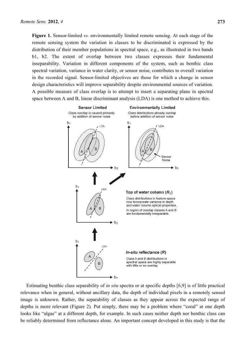
Figure 2. Hypothetical stylised example to illustrate the need to assess separability of

benthic classes across a depth range. Above water reflectance measured in two bands

(b1, b2) shows the basic within-class variance in in situ reflectances of two benthic classes

(A and B) shifted at the specific depths 1, 2 and 3 m, (a) and (b). Any pair-wise

comparison between A and B at two specific depths indicates high separability ~65% (c).

However, given that A and B can occur at any depth, for very few values of b1 and b2 can

the benthic class be unequivocally identified as A or B and the actual separability of A and

B is very low ~15% (d). Pair-wise comparisons (c) cannot be combined to reveal the

overall separability (d) since there is no way to know that the individual overlap regions

combine to give (d).

The recent trend in analysis algorithms for shallow water benthic remote sensing is to seek a

pixel-by-pixel best fit for reflectance from a forward-based radiative transfer model parameterised on

benthic reflectance, depth, water optical properties [12,14–21]. Such algorithms offer the promise of

simultaneous derivation of depth, water optical properties and benthic class. However, clearly, within


275

such multi-parameter models there is the possibility for confusion, where different sets of parameters

produce similar predicted reflectances. This issue is another expression of the concept of a system

being “environmentally limited” (Figure 1).

Various authors have discussed the possibility of a new satellite-based remote sensing instrument

designed specifically for coral reef applications [6,7,10]. While these studies have focused on

determining optimal band wavelengths, further work is now needed to provide concrete design advice

on issues such as the trade-off between spatial resolution, spectral resolution and SNR. To justify

expenditure on a new satellite sensor considerable effort must be made to evaluate the expected

efficacy of the proposed design, this requires a credible assessment of the extent to which sources of

environmental variance are inherently limiting. In this paper we present a methodology designed to

address this question, and as first step apply it to an airborne sensor configuration with a fixed set of

spectral bands (Table 1). We consider the optimal SNR and relative spatial resolution in relation to reef

heterogeneity for detection of coral bleaching, mortality and algal overgrowth of live coral on a Pacific

reef. While this study concentrates on reef-scale monitoring at high spatial resolutions, the limits of

discrimination established are also directly relevant to satellite sensors, and the methodology is readily

extendable to include atmospheric effects and different spectral band assignments.

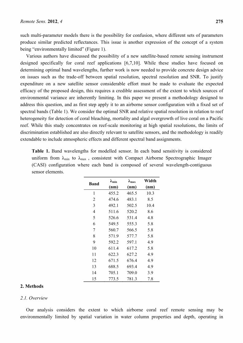
Table 1. Band wavelengths for modelled sensor. In each band sensitivity is considered

uniform from λmin to λmax , consistent with Compact Airborne Spectrographic Imager

(CASI) configuration where each band is composed of several wavelength-contiguous

sensor elements.

Band λmin λmax Width

(nm) (nm) (nm)

1 455.2 465.5 10.3 2 474.6 483.1 8.5 3 492.1 502.5 10.4 4 511.6 520.2 8.6 5 526.6 531.4 4.8 6 549.5 555.3 5.8 7 560.7 566.5 5.8 8 571.9 577.7 5.8 9 592.2 597.1 4.9

10 611.4 617.2 5.8 11 622.3 627.2 4.9 12 671.5 676.4 4.9 13 688.5 693.4 4.9 14 705.1 709.0 3.9 15 773.5 781.3 7.8

2. Methods

2.1. Overview

Our analysis considers the extent to which airborne coral reef remote sensing may be

environmentally limited by spatial variation in water column properties and depth, operating in


276

conjunction with other environmental factors such as sub-pixel mixing from benthic classes of mixed

composition, i.e., spatial resolution vs. heterogeneity, sea surface state and sun elevation (Figure 3(b)).

A modelling and sensitivity analysis was performed in which the spectral separability of benthic

classes was assessed under a set of scenarios each representing a different combination of environmental

factors and sensor characteristics. By comparing achievable separability under different scenarios the

effects of individual environmental factors were assessed, such as the difference between separability

at specific depths as opposed to separability when the benthic classes occur across a range of depths.

Previous work has considered sensor spectral band configurations for coral reef applications [6,7]. For

statistical validity, given the large number of degrees of freedom in configuring a hyperspectral sensor,

this requires a very substantial dataset of reflectances (i.e., 1,000’s). So to simplify the analysis here,

we used a single configuration of sensor wavelength bands throughout (Table 1) and concentrate on

sensor noise and sub-pixel mixing, the latter being analogous to the effect of spatial resolution. The

band choices are based on a review of coral and algal pigment absorption features from spectroscopy

and remote sensing [4], and actual configurations of the Compact Airborne Spectrographic Imager

(CASI) used in previous studies which have demonstrated discrimination of live and dead coral [2,3].

The structure of the methods and analysis are summarised in the flowchart of Figure 3(a), and the

details are presented in the following sections.

2.2. Sensitivity Analysis Structure

The sensitivity analysis involved modelling the distribution of sensor recorded spectral reflectance

for each benthic class under specific scenarios defined by the other environmental and sensor factors.

Note we use the term “scenario” to represent a particular combination of environmental factors and

sensor configuration (Figure 3(b), Table 2). The separability of the reflectance distributions for differing

benthic compositions (Figure 1) under a given class combination scenario indicates the extent to which

that particular combination of environmental factors and sensor configuration confounded separability

for those benthic classes.

In the benthic remote sensing literature the concept of “class” is often restricted to benthos, since

“classification” of image pixels to benthic classes is usually the final aim [22]. However, as Mobley [23]

discusses, the translation of class structured analyses as used in terrestrial applications to sub-surface

aquatic environments is problematic, since benthic composition is only one of several environmental

and sensor factors that contribute to the sensor recorded signal. In our analysis we conceive a class

structure for the other environmental factors and sensor configurations (Table 2). For example, in the

same way that the pure Live Coral benthic class was modelled as a set of reflectance spectra from live

corals, the Zonal IOP class was modelled as a set of water optical properties collected across different

reef zone locations. This is conceptually similar to the structure of image analysis methods which use

look up tables or model inversions based on a range of water optical properties [16,18] but here some

classes are explicitly constructed to encompass within-class variance of the parameters in question. By

this method, parameters often treated as quantitative, such as depth [16] can be class structured by

quantizing the value range in a manner suitable for the application and then grouping discrete values

into classes (Table 2).


277

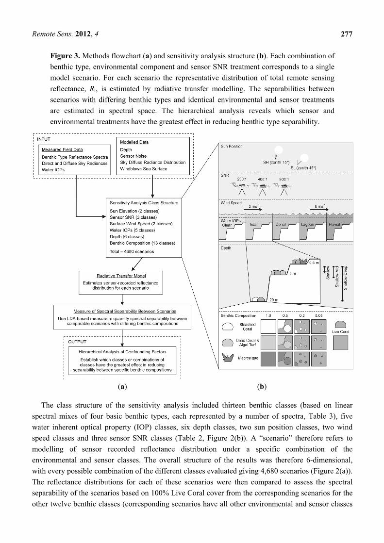
Figure 3. Methods flowchart (a) and sensitivity analysis structure (b). Each combination of

benthic type, environmental component and sensor SNR treatment corresponds to a single

model scenario. For each scenario the representative distribution of total remote sensing

reflectance, Rt, is estimated by radiative transfer modelling. The separabilities between

scenarios with differing benthic types and identical environmental and sensor treatments

are estimated in spectral space. The hierarchical analysis reveals which sensor and

environmental treatments have the greatest effect in reducing benthic type separability.

(a) (b)

The class structure of the sensitivity analysis included thirteen benthic classes (based on linear

spectral mixes of four basic benthic types, each represented by a number of spectra, Table 3), five

water inherent optical property (IOP) classes, six depth classes, two sun position classes, two wind

speed classes and three sensor SNR classes (Table 2, Figure 2(b)). A “scenario” therefore refers to

modelling of sensor recorded reflectance distribution under a specific combination of the

environmental and sensor classes. The overall structure of the results was therefore 6-dimensional,

with every possible combination of the different classes evaluated giving 4,680 scenarios (Figure 2(a)).

The reflectance distributions for each of these scenarios were then compared to assess the spectral

separability of the scenarios based on 100% Live Coral cover from the corresponding scenarios for the

other twelve benthic classes (corresponding scenarios have all other environmental and sensor classes


278

the same). This gave a total of 4,320 individual separability evaluations: three groups of 1,440

scenarios corresponding to discrimination of pure Live Coral from mixtures containing Bleached

Coral, Dead Coral/Turf and Macroalgae respectively. For each of these three benthic class groups a

hierarchical master analysis (described below) organised the 1,440 results into a graph diagram

structure revealing the most significant environmental and sensor classes with respect to reducing the

separability of the benthic compositions from pure Live Coral.

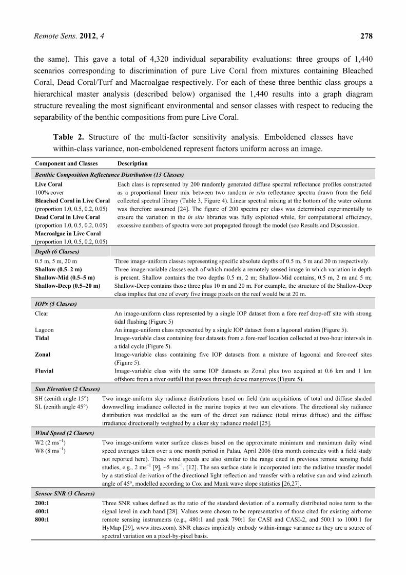
Table 2. Structure of the multi-factor sensitivity analysis. Emboldened classes have

within-class variance, non-emboldened represent factors uniform across an image.

Component and Classes Description

Benthic Composition Reflectance Distribution (13 Classes)

Live Coral 100% cover

Each class is represented by 200 randomly generated diffuse spectral reflectance profiles constructed as a proportional linear mix between two random in situ reflectance spectra drawn from the field collected spectral library (Table 3, Figure 4). Linear spectral mixing at the bottom of the water column was therefore assumed [24]. The figure of 200 spectra per class was determined experimentally to ensure the variation in the in situ libraries was fully exploited while, for computational efficiency, excessive numbers of spectra were not propagated through the model (see Results and Discussion.

Bleached Coral in Live Coral (proportion 1.0, 0.5, 0.2, 0.05) Dead Coral in Live Coral (proportion 1.0, 0.5, 0.2, 0.05) Macroalgae in Live Coral (proportion 1.0, 0.5, 0.2, 0.05)

Depth (6 Classes)

0.5 m, 5 m, 20 m Three image-uniform classes representing specific absolute depths of 0.5 m, 5 m and 20 m respectively. Shallow (0.5–2 m) Shallow-Mid (0.5–5 m) Shallow-Deep (0.5–20 m)

Three image-variable classes each of which models a remotely sensed image in which variation in depth is present. Shallow contains the two depths 0.5 m, 2 m; Shallow-Mid contains, 0.5 m, 2 m and 5 m; Shallow-Deep contains those three plus 10 m and 20 m. For example, the structure of the Shallow-Deep class implies that one of every five image pixels on the reef would be at 20 m.

IOPs (5 Classes)

Clear An image-uniform class represented by a single IOP dataset from a fore reef drop-off site with strong tidal flushing (Figure 5)

Lagoon An image-uniform class represented by a single IOP dataset from a lagoonal station (Figure 5). Tidal Image-variable class containing four datasets from a fore-reef location collected at two-hour intervals in

a tidal cycle (Figure 5). Zonal Image-variable class containing five IOP datasets from a mixture of lagoonal and fore-reef sites

(Figure 5). Fluvial Image-variable class with the same IOP datasets as Zonal plus two acquired at 0.6 km and 1 km

offshore from a river outfall that passes through dense mangroves (Figure 5).

Sun Elevation (2 Classes)

SH (zenith angle 15°) SL (zenith angle 45°)

Two image-uniform sky radiance distributions based on field data acquisitions of total and diffuse shaded downwelling irradiance collected in the marine tropics at two sun elevations. The directional sky radiance distribution was modelled as the sum of the direct sun radiance (total minus diffuse) and the diffuse irradiance directionally weighted by a clear sky radiance model [25].

Wind Speed (2 Classes)

W2 (2 ms−1) W8 (8 ms−1)

Two image-uniform water surface classes based on the approximate minimum and maximum daily wind speed averages taken over a one month period in Palau, April 2006 (this month coincides with a field study not reported here). These wind speeds are also similar to the range cited in previous remote sensing field studies, e.g., 2 ms−1 [9], ~5 ms−1, [12]. The sea surface state is incorporated into the radiative transfer model by a statistical derivation of the directional light reflection and transfer with a relative sun and wind azimuth angle of 45°, modelled according to Cox and Munk wave slope statistics [26,27].

Sensor SNR (3 Classes)

200:1 400:1 800:1

Three SNR values defined as the ratio of the standard deviation of a normally distributed noise term to the signal level in each band [28]. Values were chosen to be representative of those cited for existing airborne remote sensing instruments (e.g., 480:1 and peak 790:1 for CASI and CASI-2, and 500:1 to 1000:1 for HyMap [29], www.itres.com). SNR classes implicitly embody within-image variance as they are a source of spectral variation on a pixel-by-pixel basis.


279

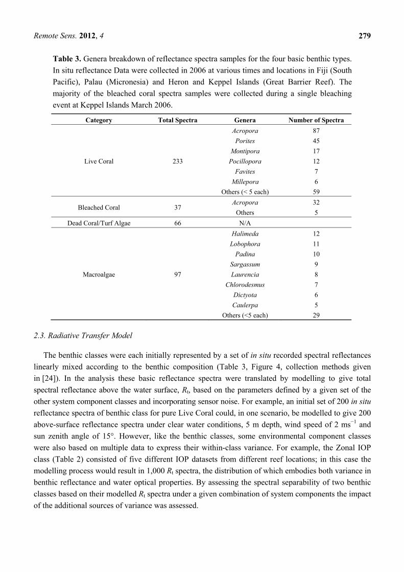
Table 3. Genera breakdown of reflectance spectra samples for the four basic benthic types.

In situ reflectance Data were collected in 2006 at various times and locations in Fiji (South

Pacific), Palau (Micronesia) and Heron and Keppel Islands (Great Barrier Reef). The

majority of the bleached coral spectra samples were collected during a single bleaching

event at Keppel Islands March 2006.

Category Total Spectra Genera Number of Spectra

Live Coral 233

Acropora

Porites

Montipora

Pocillopora

Favites

Millepora

Others (< 5 each)

87

45

17

12

7

6

59

Bleached Coral 37 Acropora

Others

32

5

Dead Coral/Turf Algae 66 N/A

Macroalgae 97

Halimeda

Lobophora

Padina

Sargassum

Laurencia

Chlorodesmus

Dictyota

Caulerpa

Others (<5 each)

12

11

10

9

8

7

6

5

29

2.3. Radiative Transfer Model

The benthic classes were each initially represented by a set of in situ recorded spectral reflectances

linearly mixed according to the benthic composition (Table 3, Figure 4, collection methods given

in [24]). In the analysis these basic reflectance spectra were translated by modelling to give total

spectral reflectance above the water surface, Rt, based on the parameters defined by a given set of the

other system component classes and incorporating sensor noise. For example, an initial set of 200 in situ

reflectance spectra of benthic class for pure Live Coral could, in one scenario, be modelled to give 200

above-surface reflectance spectra under clear water conditions, 5 m depth, wind speed of 2 ms−1 and

sun zenith angle of 15°. However, like the benthic classes, some environmental component classes

were also based on multiple data to express their within-class variance. For example, the Zonal IOP

class (Table 2) consisted of five different IOP datasets from different reef locations; in this case the

modelling process would result in 1,000 Rt spectra, the distribution of which embodies both variance in

benthic reflectance and water optical properties. By assessing the spectral separability of two benthic

classes based on their modelled Rt spectra under a given combination of system components the impact

of the additional sources of variance was assessed.


280

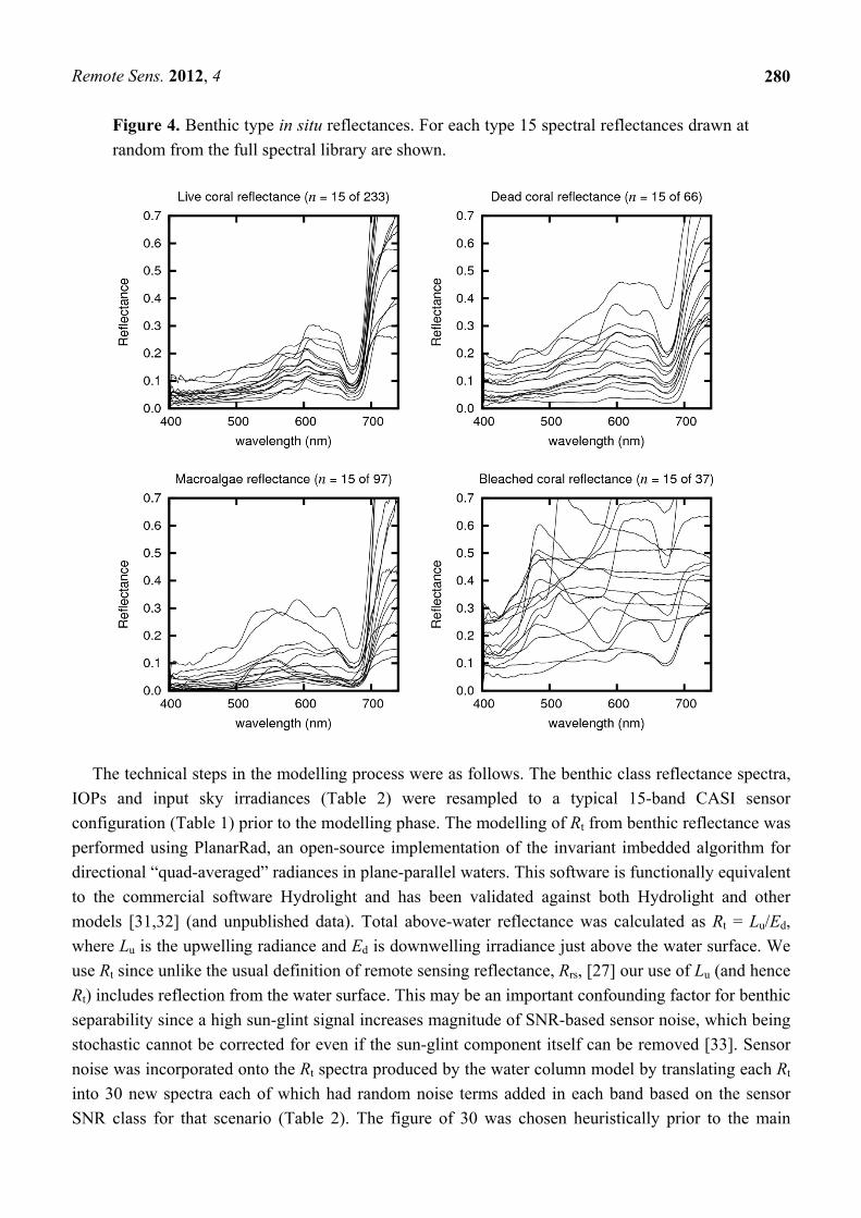
Figure 4. Benthic type in situ reflectances. For each type 15 spectral reflectances drawn at

random from the full spectral library are shown.

The technical steps in the modelling process were as follows. The benthic class reflectance spectra,

IOPs and input sky irradiances (Table 2) were resampled to a typical 15-band CASI sensor

configuration (Table 1) prior to the modelling phase. The modelling of Rt from benthic reflectance was

performed using PlanarRad, an open-source implementation of the invariant imbedded algorithm for

directional “quad-averaged” radiances in plane-parallel waters. This software is functionally equivalent

to the commercial software Hydrolight and has been validated against both Hydrolight and other

models [31,32] (and unpublished data). Total above-water reflectance was calculated as Rt = Lu/Ed,

where Lu is the upwelling radiance and Ed is downwelling irradiance just above the water surface. We

use Rt since unlike the usual definition of remote sensing reflectance, Rrs, [27] our use of Lu (and hence

Rt) includes reflection from the water surface. This may be an important confounding factor for benthic

separability since a high sun-glint signal increases magnitude of SNR-based sensor noise, which being

stochastic cannot be corrected for even if the sun-glint component itself can be removed [33]. Sensor

noise was incorporated onto the Rt spectra produced by the water column model by translating each Rt

into 30 new spectra each of which had random noise terms added in each band based on the sensor

SNR class for that scenario (Table 2). The figure of 30 was chosen heuristically prior to the main


281

analysis with the objective being to fully populate the signal noise in the 15-band spectral space

without excessive redundancy.

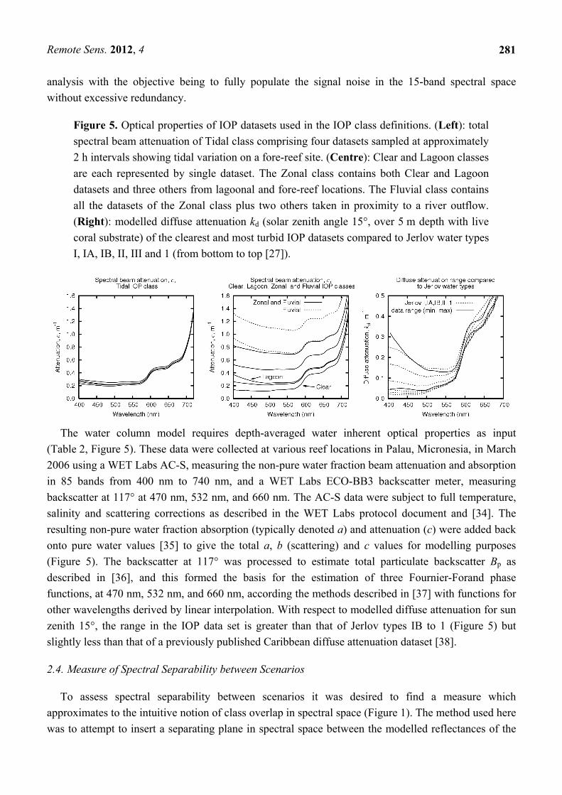
Figure 5. Optical properties of IOP datasets used in the IOP class definitions. (Left): total

spectral beam attenuation of Tidal class comprising four datasets sampled at approximately

2 h intervals showing tidal variation on a fore-reef site. (Centre): Clear and Lagoon classes

are each represented by single dataset. The Zonal class contains both Clear and Lagoon

datasets and three others from lagoonal and fore-reef locations. The Fluvial class contains

all the datasets of the Zonal class plus two others taken in proximity to a river outflow.

(Right): modelled diffuse attenuation kd (solar zenith angle 15°, over 5 m depth with live

coral substrate) of the clearest and most turbid IOP datasets compared to Jerlov water types

I, IA, IB, II, III and 1 (from bottom to top [27]).

The water column model requires depth-averaged water inherent optical properties as input

(Table 2, Figure 5). These data were collected at various reef locations in Palau, Micronesia, in March

2006 using a WET Labs AC-S, measuring the non-pure water fraction beam attenuation and absorption

in 85 bands from 400 nm to 740 nm, and a WET Labs ECO-BB3 backscatter meter, measuring

backscatter at 117° at 470 nm, 532 nm, and 660 nm. The AC-S data were subject to full temperature,

salinity and scattering corrections as described in the WET Labs protocol document and [34]. The

resulting non-pure water fraction absorption (typically denoted a) and attenuation (c) were added back

onto pure water values [35] to give the total a, b (scattering) and c values for modelling purposes

(Figure 5). The backscatter at 117° was processed to estimate total particulate backscatter Bp as

described in [36], and this formed the basis for the estimation of three Fournier-Forand phase

functions, at 470 nm, 532 nm, and 660 nm, according the methods described in [37] with functions for

other wavelengths derived by linear interpolation. With respect to modelled diffuse attenuation for sun

zenith 15°, the range in the IOP data set is greater than that of Jerlov types IB to 1 (Figure 5) but

slightly less than that of a previously published Caribbean diffuse attenuation dataset [38].

2.4. Measure of Spectral Separability between Scenarios

To assess spectral separability between scenarios it was desired to find a measure which

approximates to the intuitive notion of class overlap in spectral space (Figure 1). The method used here

was to attempt to insert a separating plane in spectral space between the modelled reflectances of the


282

two benthic types (Figure 1). The inverse of the grouped covariance matrix is one way to establish

such a plane and is similar to linear discriminant analysis (LDA) [39]. For each pair of benthic classes

and a specific set of treatments (a scenario) the set of n Rt spectra representing each class was used to

establish a dividing plane in spectral space (Figure 1) and the number of individual spectra lying on

their correct class side of the plane was counted as nc. Note that nc ranges from n to 2n since there are a

total of 2n spectra and a separating plane can always be found such that half the points are on the

correct class side (Figure 1). Separability, τ, was then calculated as,

n

nn c100 (%) (1)

In practice, the range of τ is 0% (completely inseparable classes) to 100% (completely separable)

and has identical interpretation to the Tau coefficient [40] as the percentage more correct

classifications achieved than would be expected by chance alone [22]. An individual τ value has no

associated statistical significance and is simply a number that approximates to the fundamental

separability between the spectral distributions for a specific model evaluation (Figure 1).

The fully factored sensitivity analysis contained 4,680 class combinations (i.e., scenarios) that

corresponded to modelling approximately 1,560,000 Rt spectra, before the addition of sensor noise. For

each comparison between scenarios the τ value gives the resultant separability for that particular model

evaluation with no associated statistical significance. However, since some classes contained stochastic

elements, e.g., benthic class mixtures and sensor noise, the predicted separabilities are estimates of

what would be expected under many model runs for the given scenarios. To assess the spread of these

estimates the entire analysis was repeated ten times. In the results the mean separabilities () are

reported with reference to their standard error over the ten runs. Where required, t-tests were applied to

these mean separabilities to determine if an apparent change in separability were genuine or an artefact

of the specific instantiations of stochastic components of the model. Where this was done

simultaneously across several scenarios both the standard and Dunn-Ŝidák Type I error corrected

results were calculated [41].

2.5. Hierarchical Analysis of Confounding Factors

With 4,680 class combinations in a 6-dimensional results table further condensing of the results is

required to get an overview of relative importance of the different factors. Here we present a general

method of constructing a hierarchical class significance diagram from a fully factorised sensitivity

analysis (Figure 6).

The diagram consists of a directed graph (meaning “graph” as in graph theory [42]) that is built

starting with a single vertex representing the entire results, i.e., all scenarios, and then scenarios

including specific classes are iteratively excluded with the classes chosen in order to maximally

increase the overall accuracy at each step. The result is a directed graph where each arc represents the

exclusion of a class from the entire results table and vertices represent the resulting subsets of

scenarios. The vertical position of a vertex in the diagram is based on the mean separability over the

set of scenarios that it represents. Therefore the relative effect of excluding successive confounding

classes is readily apparent. The horizontal position of vertices has no meaning and is merely based on

spacing out the vertices at each level. The graph is built iteratively, for each current vertex each class is


283

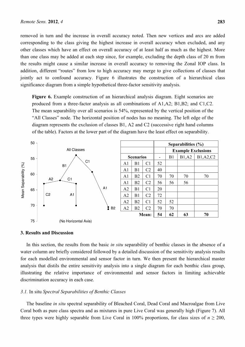
removed in turn and the increase in overall accuracy noted. Then new vertices and arcs are added

corresponding to the class giving the highest increase in overall accuracy when excluded, and any

other classes which have an effect on overall accuracy of at least half as much as the highest. More

than one class may be added at each step since, for example, excluding the depth class of 20 m from

the results might cause a similar increase in overall accuracy to removing the Zonal IOP class. In

addition, different “routes” from low to high accuracy may merge to give collections of classes that

jointly act to confound accuracy. Figure 6 illustrates the construction of a hierarchical class

significance diagram from a simple hypothetical three-factor sensitivity analysis.

Figure 6. Example construction of an hierarchical analysis diagram. Eight scenarios are

produced from a three-factor analysis as all combinations of A1,A2; B1,B2; and C1,C2.

The mean separability over all scenarios is 54%, represented by the vertical position of the

“All Classes” node. The horizontal position of nodes has no meaning. The left edge of the

diagram represents the exclusion of classes B1, A2 and C2 (successive right hand columns

of the table). Factors at the lower part of the diagram have the least effect on separability.

Separabilities (%)

Example Exclusions

Scenarios - B1 B1,A2 B1,A2,C2

A1 B1 C1 52

A1 B1 C2 40

A1 B2 C1 70 70 70 70

A1 B2 C2 56 56 56

A2 B1 C1 20

A2 B1 C2 72

A2 B2 C1 52 52

A2 B2 C2 70 70

Mean: 54 62 63 70

3. Results and Discussion

In this section, the results from the basic in situ separability of benthic classes in the absence of a

water column are briefly considered followed by a detailed discussion of the sensitivity analysis results

for each modelled environmental and sensor factor in turn. We then present the hierarchical master

analysis that distils the entire sensitivity analysis into a single diagram for each benthic class group,

illustrating the relative importance of environmental and sensor factors in limiting achievable

discrimination accuracy in each case.

3.1. In situ Spectral Separabilities of Benthic Classes

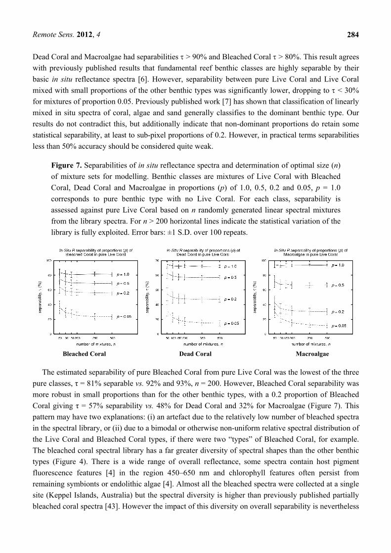
The baseline in situ spectral separability of Bleached Coral, Dead Coral and Macroalgae from Live

Coral both as pure class spectra and as mixtures in pure Live Coral was generally high (Figure 7). All

three types were highly separable from Live Coral in 100% proportions, for class sizes of n ≥ 200,


284

Dead Coral and Macroalgae had separabilities > 90% and Bleached Coral > 80%. This result agrees

with previously published results that fundamental reef benthic classes are highly separable by their

basic in situ reflectance spectra [6]. However, separability between pure Live Coral and Live Coral

mixed with small proportions of the other benthic types was significantly lower, dropping to < 30%

for mixtures of proportion 0.05. Previously published work [7] has shown that classification of linearly

mixed in situ spectra of coral, algae and sand generally classifies to the dominant benthic type. Our

results do not contradict this, but additionally indicate that non-dominant proportions do retain some

statistical separability, at least to sub-pixel proportions of 0.2. However, in practical terms separabilities

less than 50% accuracy should be considered quite weak.

Figure 7. Separabilities of in situ reflectance spectra and determination of optimal size (n)

of mixture sets for modelling. Benthic classes are mixtures of Live Coral with Bleached

Coral, Dead Coral and Macroalgae in proportions (p) of 1.0, 0.5, 0.2 and 0.05, p = 1.0

corresponds to pure benthic type with no Live Coral. For each class, separability is

assessed against pure Live Coral based on n randomly generated linear spectral mixtures

from the library spectra. For n > 200 horizontal lines indicate the statistical variation of the

library is fully exploited. Error bars: ±1 S.D. over 100 repeats.

Bleached Coral Dead Coral Macroalgae

The estimated separability of pure Bleached Coral from pure Live Coral was the lowest of the three

pure classes, τ = 81% separable vs. 92% and 93%, n = 200. However, Bleached Coral separability was

more robust in small proportions than for the other benthic types, with a 0.2 proportion of Bleached

Coral giving τ = 57% separability vs. 48% for Dead Coral and 32% for Macroalgae (Figure 7). This

pattern may have two explanations: (i) an artefact due to the relatively low number of bleached spectra

in the spectral library, or (ii) due to a bimodal or otherwise non-uniform relative spectral distribution of

the Live Coral and Bleached Coral types, if there were two “types” of Bleached Coral, for example.

The bleached coral spectral library has a far greater diversity of spectral shapes than the other benthic

types (Figure 4). There is a wide range of overall reflectance, some spectra contain host pigment

fluorescence features [4] in the region 450–650 nm and chlorophyll features often persist from

remaining symbionts or endolithic algae [4]. Almost all the bleached spectra were collected at a single

site (Keppel Islands, Australia) but the spectral diversity is higher than previously published partially

bleached coral spectra [43]. However the impact of this diversity on overall separability is nevertheless


285

small since τ = 81% still predicts pure Bleached Coral and Live Coral to be highly separable.

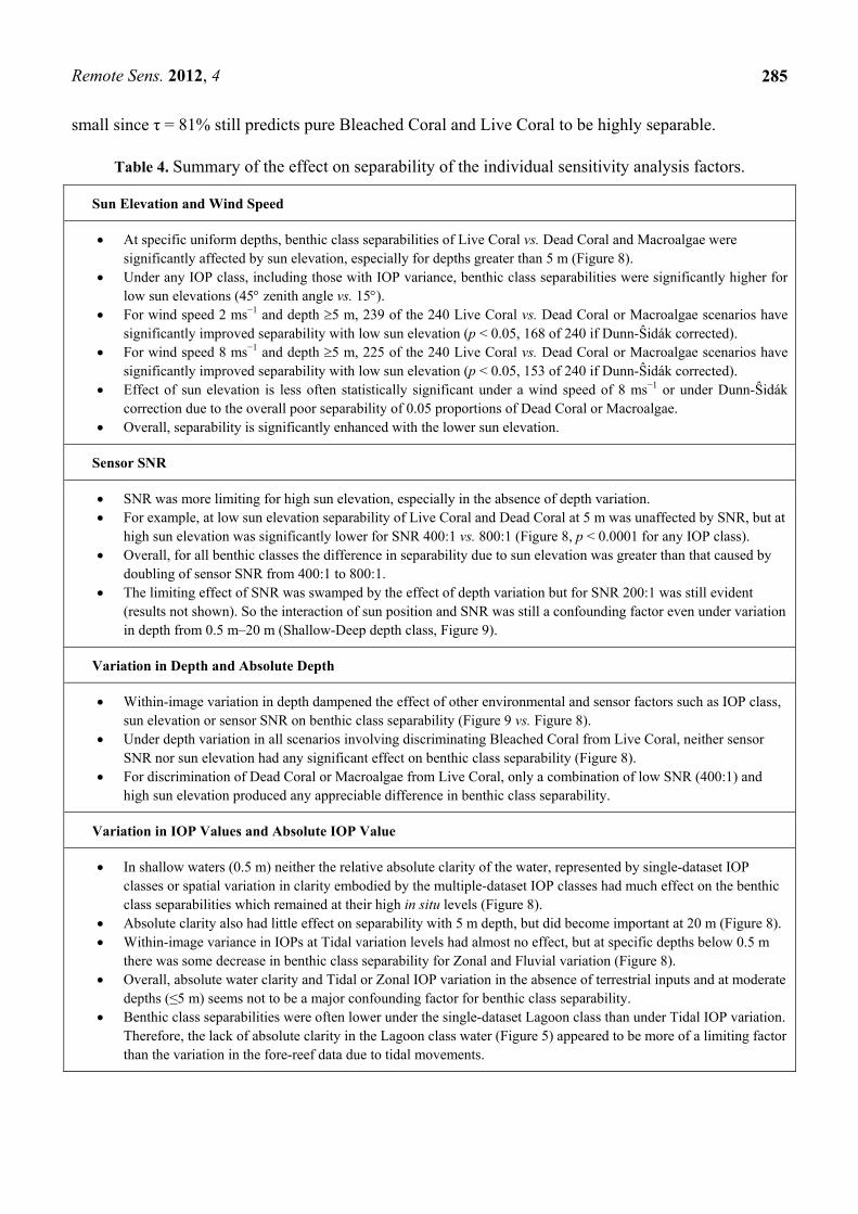
Table 4. Summary of the effect on separability of the individual sensitivity analysis factors.

Sun Elevation and Wind Speed

At specific uniform depths, benthic class separabilities of Live Coral vs. Dead Coral and Macroalgae were significantly affected by sun elevation, especially for depths greater than 5 m (Figure 8).

Under any IOP class, including those with IOP variance, benthic class separabilities were significantly higher for low sun elevations (45 zenith angle vs. 15).

For wind speed 2 ms−1 and depth 5 m, 239 of the 240 Live Coral vs. Dead Coral or Macroalgae scenarios have significantly improved separability with low sun elevation (p < 0.05, 168 of 240 if Dunn-Ŝidák corrected).

For wind speed 8 ms−1 and depth 5 m, 225 of the 240 Live Coral vs. Dead Coral or Macroalgae scenarios have significantly improved separability with low sun elevation (p < 0.05, 153 of 240 if Dunn-Ŝidák corrected).

Effect of sun elevation is less often statistically significant under a wind speed of 8 ms−1 or under Dunn-Ŝidák correction due to the overall poor separability of 0.05 proportions of Dead Coral or Macroalgae.

Overall, separability is significantly enhanced with the lower sun elevation.

Sensor SNR

SNR was more limiting for high sun elevation, especially in the absence of depth variation. For example, at low sun elevation separability of Live Coral and Dead Coral at 5 m was unaffected by SNR, but at

high sun elevation was significantly lower for SNR 400:1 vs. 800:1 (Figure 8, p < 0.0001 for any IOP class). Overall, for all benthic classes the difference in separability due to sun elevation was greater than that caused by

doubling of sensor SNR from 400:1 to 800:1. The limiting effect of SNR was swamped by the effect of depth variation but for SNR 200:1 was still evident

(results not shown). So the interaction of sun position and SNR was still a confounding factor even under variation in depth from 0.5 m–20 m (Shallow-Deep depth class, Figure 9).

Variation in Depth and Absolute Depth

Within-image variation in depth dampened the effect of other environmental and sensor factors such as IOP class, sun elevation or sensor SNR on benthic class separability (Figure 9 vs. Figure 8).

Under depth variation in all scenarios involving discriminating Bleached Coral from Live Coral, neither sensor SNR nor sun elevation had any significant effect on benthic class separability (Figure 8).

For discrimination of Dead Coral or Macroalgae from Live Coral, only a combination of low SNR (400:1) and high sun elevation produced any appreciable difference in benthic class separability.

Variation in IOP Values and Absolute IOP Value

In shallow waters (0.5 m) neither the relative absolute clarity of the water, represented by single-dataset IOP classes or spatial variation in clarity embodied by the multiple-dataset IOP classes had much effect on the benthic class separabilities which remained at their high in situ levels (Figure 8).

Absolute clarity also had little effect on separability with 5 m depth, but did become important at 20 m (Figure 8). Within-image variance in IOPs at Tidal variation levels had almost no effect, but at specific depths below 0.5 m

there was some decrease in benthic class separability for Zonal and Fluvial variation (Figure 8). Overall, absolute water clarity and Tidal or Zonal IOP variation in the absence of terrestrial inputs and at moderate

depths (≤5 m) seems not to be a major confounding factor for benthic class separability. Benthic class separabilities were often lower under the single-dataset Lagoon class than under Tidal IOP variation.

Therefore, the lack of absolute clarity in the Lagoon class water (Figure 5) appeared to be more of a limiting factor than the variation in the fore-reef data due to tidal movements.


286

3.2. Individual Effect of Environmental and Sensor Factors

Estimated benthic class separabilities across the sensitivity analysis are the result of the interaction

of all the modelled factors of benthic composition, sun elevation, wind speed, absolute depth, depth

variation, absolute water clarity and variation in water clarity (Figures 8 and 9). Although strictly

speaking each factor cannot be treated in isolation, some generalisations can be made. Basic trends and

interesting observations are summarised in Table 4 and will be discussed briefly in this section.

In general, separability was significantly enhanced at the lower sun position zenith angle of 45° vs.

15° but variation in depth or low cover proportions are more severely limiting and reduced the

beneficial effect (Table 4, Figures 8 and 9). Nevertheless t-tests indicated that the majority of Live

Coral vs. Dead Coral or Macroalgae scenarios have significantly improved separability with low sun

elevation (Table 4).

The physical basis of the advantage of low sun elevation is in reduced reflection from the air-water

interface into upward radiance, Lu. For high sun elevations the benthic component is a smaller fraction

of the overall larger upwelling radiance and so is increasingly obscured by sensor signal-dependent

noise (SNR). This is supported by the results, however while for specific depths SNR was more

limiting at high sun elevation, the effect of sun elevation itself is a greater (Figure 8). Further, when the

distribution of modelled spectral reflectances (Rt) included within-image depth variation (Figure 9) the

difference in separability due to sun elevation seen at specific depths (Figure 8) was almost completely

absent although some SNR limitation at 400:1 and 200:1 (not shown) is still evident. These results are

consistent with those presented in [9] for a simple scenario based on a HyMap image and Case 1

waters. In that study the combined sensor and environmental noise, SNRE, in a HyMap image differed

from 100:1 to 20:1 in the presence of sun glint, and consequently the calculation of theoretical depth at

which live coral vs. dead coral can be discriminated in the clearest Case 1 reef waters is 25 m vs. 8 m,

respectively. This result is comparable to a single class combination in our analysis, for the Clear IOP

class, separability of Live Coral and Dead Coral at specific depth 5 m under high sun position (86%) is

the same as at specific depth 20 m for low sun position (87%) but substantially lower with high sun

position at 20 m (56%) (Figure 8, wind speed 2 ms−1, SNR 800:1). However the cited study [9] did not

consider the contribution to environmental noise (SNRE) of spatial variance in IOPs or depth and also

did not assess the possibility of across-depth confusion between benthic classes. These factors are

incorporated into our analysis by the other treatment combinations (Table 4), and show that this

specific-depth clear water result is a best case scenario for live and dead coral discrimination.

3.3. Effect of Variation in Depth vs. Absolute Depth

In a practical remote sensing application, the spectral distribution of above-water reflectances for a

given benthic class will be subject to variance caused by differences in depth. If the depth at given

pixel is unknown, the spectral reflectance could represent any benthic class at any depth within the

image depth range (Figure 2). In the sensitivity analysis this corresponds to the situation where the sets

of Rt representing benthic classes are modelled under a scenario involving one of the multiple-depth

classes Shallow, Shallow-Mid or Shallow-Deep (Table 2). Spectral variation caused by depth variation

is in itself likely to decrease the separability of the benthic classes (Figure 1). In contrast, the limiting


287

role of absolute depth, assessed as benthic class separability at a specific uniform depth, occurs only in

conjunction with other sources of variance. For example in deep water, differences in spectral

reflectance may be lower than sensor SNR thresholds, so the variance due to SNR is the fundamental

cause of the inseparability. The effect of depth on separability therefore operates by two distinct

mechanisms and variance in depth may in itself be limiting by increasing across-depth confusion

between classes irrespective of sensor SNR (Figure 1). This reasoning is supported by the results,

where the effect of variance in depth in general overwhelms the effects due to IOP class, sun elevation

or sensor SNR (Table 4, Figure 9). In particular, the strong effect of sensor SNR seen at specific

absolute depths below 5 m (Figure 8) is largely absent under depth variation (Figure 9), so attainable

accuracy is no longer “sensor limited” but is “environmentally limited” (upper right hand part of

Figure 1).

Although variation in depth reduced the significance of other factors such as sensor SNR on benthic

class separability, determining the overall effect of depth variance itself, as an isolated concept, on

achievable accuracy is less straightforward. From Figures 8 and 9 it appears as though overall

separability under the multiple-depth classes might simply be the average separability under the

specific depths within those classes. For example, if DEEPS is separability under the Shallow-Deep multiple-depth class and d is separability at specific depth d m, then maybe

5/2010525.0 DEEPS , since the Shallow-Deep class is constructed from the five

specific depths 0.5, 2, 5, 10 and 20 m (Table 2). If the above relation were true then there would be no

evidence for across-depth confusion between benthic classes and the effect of variation in depth could

simply be interpreted in terms of the separabilities at the specific absolute depths involved. In fact,

with respect to discriminating Live Coral from any of the other classes in pure 1.0 proportion, in 294

of 360 cases across the entire analysis the separability estimate under a multiple-depth class was

significantly worse than the mean separability of the corresponding individual depths (p < 0.01,

Dunn-Ŝidák correction applied). Separability results for many of the benthic classes with mixture

proportions less than 1.0 were similarly conclusive, with the pattern only breaking down for low

mixture proportions of 0.2 and 0.05, which have very low separabilities anyway.

One caveat to be considered is that the decrease in separability observed under depth variation may

be an artefact of the linear separating plane (Figure 1) if depth variation produced a curved pattern of

reflectance distribution in spectral space. In this case less constrained analysis methods such as

successive approximation or lookup tables [17,18,20] or by applying a linearising pre-classification

transform [44]. However, although the non-linear distribution argument will have some validity in

general, it is an unlikely explanation of the observed results in this case for two reasons: (i) the Shallow

multiple-depth class only contains two depths so depth variation alone cannot cause a non-linear

distribution of Rt; and (ii) variation in IOPs would be expected to produce a similar non-linear effect in

spectral distributions, but in fact in this study variation in IOPs had relatively less effect on separability

than variation in depth (Figures 8 and 9).

In a practical application, sources of environmental noise other than depth variation will be present

and may also be limiting, for example atmospheric effects, which we neglect here. Our results indicate

that it may be necessary to re-evaluate conclusions from previous studies that only consider differences

between benthic types at specific uniform water depths without possibility of across-depth confusion [9].


288

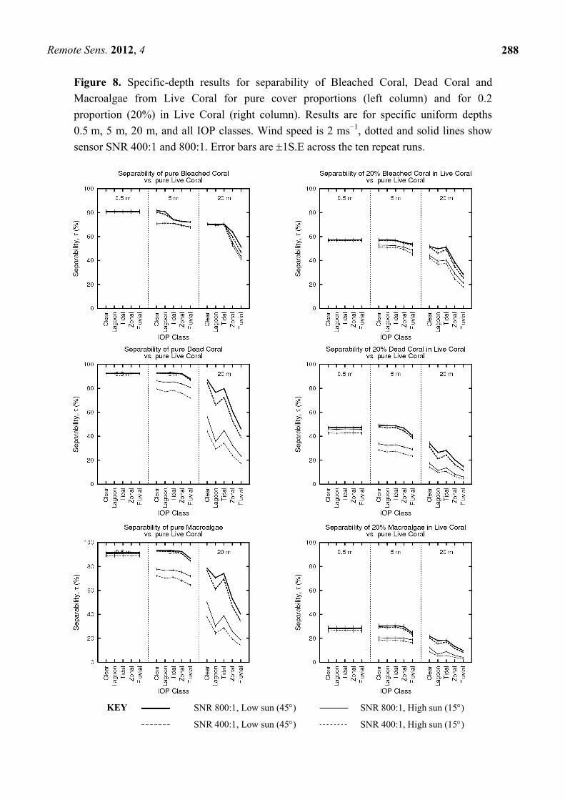
Figure 8. Specific-depth results for separability of Bleached Coral, Dead Coral and

Macroalgae from Live Coral for pure cover proportions (left column) and for 0.2

proportion (20%) in Live Coral (right column). Results are for specific uniform depths

0.5 m, 5 m, 20 m, and all IOP classes. Wind speed is 2 ms−1, dotted and solid lines show

sensor SNR 400:1 and 800:1. Error bars are 1S.E across the ten repeat runs.

KEY SNR 800:1, Low sun (45) SNR 800:1, High sun (15)

SNR 400:1, Low sun (45) SNR 400:1, High sun (15)


289

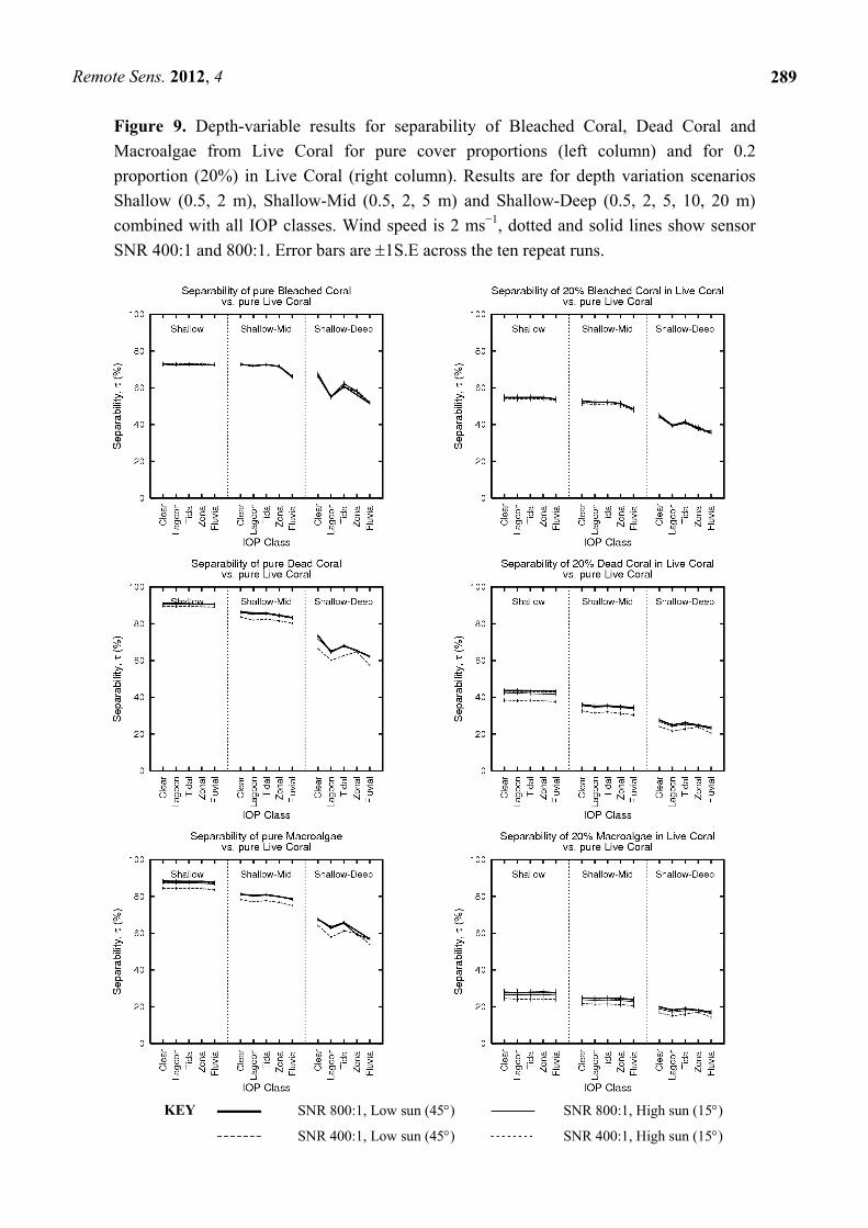
Figure 9. Depth-variable results for separability of Bleached Coral, Dead Coral and

Macroalgae from Live Coral for pure cover proportions (left column) and for 0.2

proportion (20%) in Live Coral (right column). Results are for depth variation scenarios

Shallow (0.5, 2 m), Shallow-Mid (0.5, 2, 5 m) and Shallow-Deep (0.5, 2, 5, 10, 20 m)

combined with all IOP classes. Wind speed is 2 ms−1, dotted and solid lines show sensor

SNR 400:1 and 800:1. Error bars are 1S.E across the ten repeat runs.

KEY SNR 800:1, Low sun (45) SNR 800:1, High sun (15)

SNR 400:1, Low sun (45) SNR 400:1, High sun (15)


290

Finally, by way of a comparison to field-based data, we consider a published Pacific study [3] that

demonstrated an improved ability to discriminate live from dead coral in approximate depth ranges of

2–3 m vs. 3–4 m in a 0.25 m pixel CASI image (SNR ~400:1) collected with solar zenith angle ~50°.

In contrast, the modelling results here indicate no difference in separability for these classes in clear or

lagoonal waters at specific depths of 0.5 m and 5 m for sun zenith 45° but a clear significant difference

for sun zenith 15° or waters of lower clarity (Figure 8, centre left). However, the imagery in the

published study [3] had only 6 spectral bands so our relative over-prediction of separability in the

deeper waters may be due to the higher 15-band spectral resolution in the model. Extending the model

framework to incorporate different spectral sensor configurations will answer this question and is a

priority for future work.

3.4. Effect of Variation in IOP Values vs. Absolute IOP Values

Analogous to the previous discussion on depth, a distinction can be drawn between the effects of

absolute water clarity on benthic class separability as opposed to the effects of variance in optical

properties within an image. While neither absolute water clarity nor variance in clarity had much effect

on benthic class separabilities in very shallow waters (0.5 m) absolute clarity within the modelled

range starts to become limiting beyond 5 m while Zonal and Fluvial levels of variance have some

effect at depths below 0.5 m (Table 4, Figure 8). Therefore, absolute water clarity and Tidal or Zonal

IOP variation in the absence of terrestrial inputs and at moderate depths (<5 m) seems not to be a

major confounding factor for benthic class separability. Since these conditions correspond to those

found for much of coral reef remote sensing objectives then suitable analysis algorithms should be able

to factor out water column effects [16,18,20,45]. Interpreting the total water column optical effect in

terms of optical depth (optical depth = depth × attenuation), then it is clear that variation in depth will

be more significant optically than the IOP variation in our dataset. Ratios between optical depths

among the three physical depths 0.5, 5 and 20 m are 4, 10 and 40. Whereas relative attenuation

between the IOP datasets has a maximum ratio of only around 10, or around 5 if the Fluvial class IOP

datasets are excluded (Figure 5). If the ratio of 5, between minimum and maximum attenuations in the

Lagoon class, is assumed as the typical range for reef remote sensing, then variation in IOPs will only

become more optically significant than variation in depth if the depth range is restricted such that

dmax/dmin < 5, for example, a depth range of 1 to 5 m or 2 to 10 m.

Discrimination of pure Bleached Coral from pure Live Coral presents an exception to the previous

observation that Tidal variation IOPs overall had little effect (Figure 8, top left). While no significant

difference exists in Bleached Coral separability under the single-dataset Clear or Lagoon classes,

= 81% in both cases, Tidal IOP variation significantly reduces separability of Bleached Coral from

Live Coral to = 74% (p < 0.001). This pattern occurs at both wind speeds (2 ms−1 and 8 ms−1) but

only for the high 800:1 SNR class and not when discriminating mixed proportions of Bleached Coral

in Live Coral less than 1.0 (Figure 8, top right). In most cases sediments in coral reef environments

will be dominated by calcium carbonate particles, and this was certainly true in our study sites where

coral sand was abundant. Since detection of coral bleaching by remote sensing is essentially detecting

a calcium carbonate “signal”, i.e., the coral skeleton with pigments removed, it is possible that

variation in suspended sediments may be a confounding factor specifically for the detection of


291

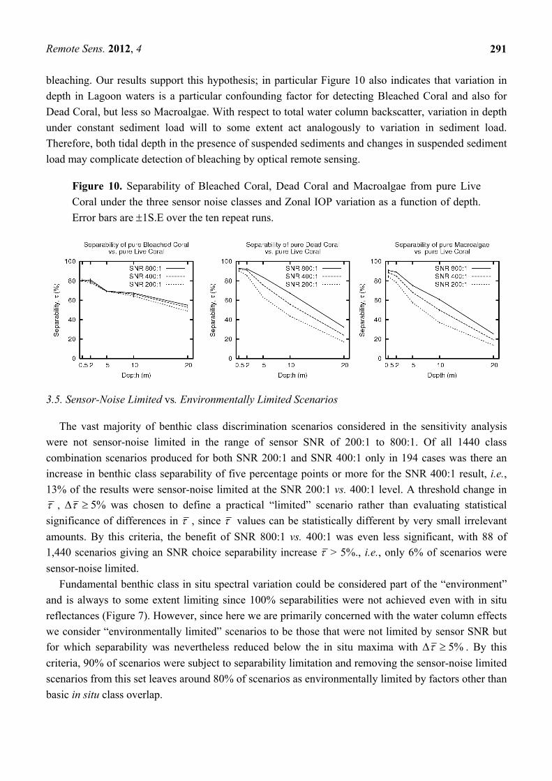
bleaching. Our results support this hypothesis; in particular Figure 10 also indicates that variation in

depth in Lagoon waters is a particular confounding factor for detecting Bleached Coral and also for

Dead Coral, but less so Macroalgae. With respect to total water column backscatter, variation in depth

under constant sediment load will to some extent act analogously to variation in sediment load.

Therefore, both tidal depth in the presence of suspended sediments and changes in suspended sediment

load may complicate detection of bleaching by optical remote sensing.

Figure 10. Separability of Bleached Coral, Dead Coral and Macroalgae from pure Live

Coral under the three sensor noise classes and Zonal IOP variation as a function of depth.

Error bars are 1S.E over the ten repeat runs.

3.5. Sensor-Noise Limited vs. Environmentally Limited Scenarios

The vast majority of benthic class discrimination scenarios considered in the sensitivity analysis

were not sensor-noise limited in the range of sensor SNR of 200:1 to 800:1. Of all 1440 class

combination scenarios produced for both SNR 200:1 and SNR 400:1 only in 194 cases was there an

increase in benthic class separability of five percentage points or more for the SNR 400:1 result, i.e.,

13% of the results were sensor-noise limited at the SNR 200:1 vs. 400:1 level. A threshold change in

, %5 was chosen to define a practical “limited” scenario rather than evaluating statistical

significance of differences in , since values can be statistically different by very small irrelevant

amounts. By this criteria, the benefit of SNR 800:1 vs. 400:1 was even less significant, with 88 of

1,440 scenarios giving an SNR choice separability increase > 5%., i.e., only 6% of scenarios were

sensor-noise limited.

Fundamental benthic class in situ spectral variation could be considered part of the “environment”

and is always to some extent limiting since 100% separabilities were not achieved even with in situ

reflectances (Figure 7). However, since here we are primarily concerned with the water column effects

we consider “environmentally limited” scenarios to be those that were not limited by sensor SNR but

for which separability was nevertheless reduced below the in situ maxima with %5 . By this

criteria, 90% of scenarios were subject to separability limitation and removing the sensor-noise limited

scenarios from this set leaves around 80% of scenarios as environmentally limited by factors other than

basic in situ class overlap.


292

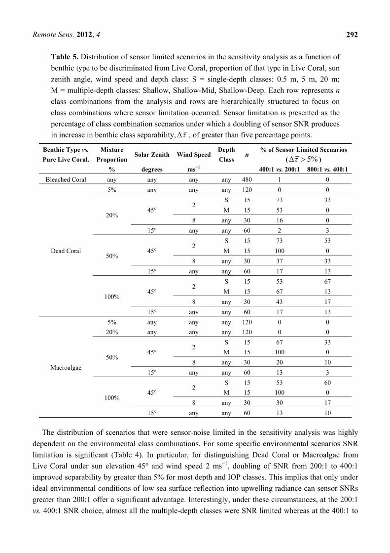
Table 5. Distribution of sensor limited scenarios in the sensitivity analysis as a function of

benthic type to be discriminated from Live Coral, proportion of that type in Live Coral, sun

zenith angle, wind speed and depth class: S = single-depth classes: 0.5 m, 5 m, 20 m;

M = multiple-depth classes: Shallow, Shallow-Mid, Shallow-Deep. Each row represents n

class combinations from the analysis and rows are hierarchically structured to focus on

class combinations where sensor limitation occurred. Sensor limitation is presented as the

percentage of class combination scenarios under which a doubling of sensor SNR produces

in increase in benthic class separability, , of greater than five percentage points.

Benthic Type vs.

Pure Live Coral.

Mixture

Proportion Solar Zenith Wind Speed

Depth

Class n

% of Sensor Limited Scenarios

( %5 )

% degrees ms−1 400:1 vs. 200:1 800:1 vs. 400:1

Bleached Coral any any any any 480 1 0

Dead Coral

5% any any any 120 0 0

20% 45°

2 S 15 73 33

M 15 53 0

8 any 30 16 0

15° any any 60 2 3

50% 45°

2 S 15 73 53

M 15 100 0

8 any 30 37 33

15° any any 60 17 13

100% 45°

2 S 15 53 67

M 15 67 13

8 any 30 43 17

15° any any 60 17 13

Macroalgae

5% any any any 120 0 0

20% any any any 120 0 0

50% 45°

2 S 15 67 33

M 15 100 0

8 any 30 20 10

15° any any 60 13 3

100% 45°

2 S 15 53 60

M 15 100 0

8 any 30 30 17

15° any any 60 13 10

The distribution of scenarios that were sensor-noise limited in the sensitivity analysis was highly

dependent on the environmental class combinations. For some specific environmental scenarios SNR

limitation is significant (Table 4). In particular, for distinguishing Dead Coral or Macroalgae from

Live Coral under sun elevation 45° and wind speed 2 ms−1, doubling of SNR from 200:1 to 400:1

improved separability by greater than 5% for most depth and IOP classes. This implies that only under

ideal environmental conditions of low sea surface reflection into upwelling radiance can sensor SNRs

greater than 200:1 offer a significant advantage. Interestingly, under these circumstances, at the 200:1

vs. 400:1 SNR choice, almost all the multiple-depth classes were SNR limited whereas at the 400:1 to


293

800:1 choice none were (Table 4). This indicates the point at which depth variation overwhelmed

sensor SNR as a confounding factor was around the SNR 400:1 level. Therefore, within the scope of

this study, variation in depth was slightly less problematic for benthic class discrimination than the

combination of sea surface state and sun elevation. Conversely, as discussed before, considering

absolute depth as modelled by the single-depth classes, sensor-noise limitation continues to be

predicted at the SNR 400:1 to 800:1 level under low sea surface reflection (Table 4). This again

reiterates the point that considering separability only at specific uniform depths will over-emphasise

the importance of sensor SNR.

Finally, note that discrimination of any mixture proportion of Bleached Coral from Live Coral was

not sensor limited under almost any class combination scenario (Table 4). This is consistent with the

earlier argument developed from the in situ results, that a large part of the Live Coral and Bleached

Coral classes are highly separable, and hence do not require high sensor SNR to be discriminated.

Unlike the Dead Coral and Macroalgae classes, the separability of Bleached Coral from Live Coral

remains quite high as absolute depth increases and is relatively insensitive to sensor SNR (Figure 10).

Therefore, different objectives within the scope coral reef remote sensing may demand different

optimal sensor designs.

3.6. Hierarchical Analysis of Confounding Factors

Hierarchical summary diagrams (Figure 6) were constructed from the 1,440 factor combination

scenarios to illustrate the relative significance of the various environmental and sensor class choices

with respect to the entire sensitivity analysis for each basic benthic type (Figures 11–13). Each

diagram should be read from top to bottom starting at the “All Scenarios” vertex, the vertical position

of which indicates the mean separability over all 1,440 scenarios. Subsequent nodes indicate the mean

separability as scenarios containing the most significant confounding factors are iteratively removed

from the analysis (labelled arcs). At the bottom region of the graphs only the “ideal” scenarios for

benthic class discrimination remain and the mean separability as represented by vertical position of the

individual vertices is close to the maximum attainable under any scenario. The following sections

discuss and interpret the patterns in these diagrams (Figures 11–13).

3.6.1. Initial Factor Exclusion—Sub-Pixel Proportions

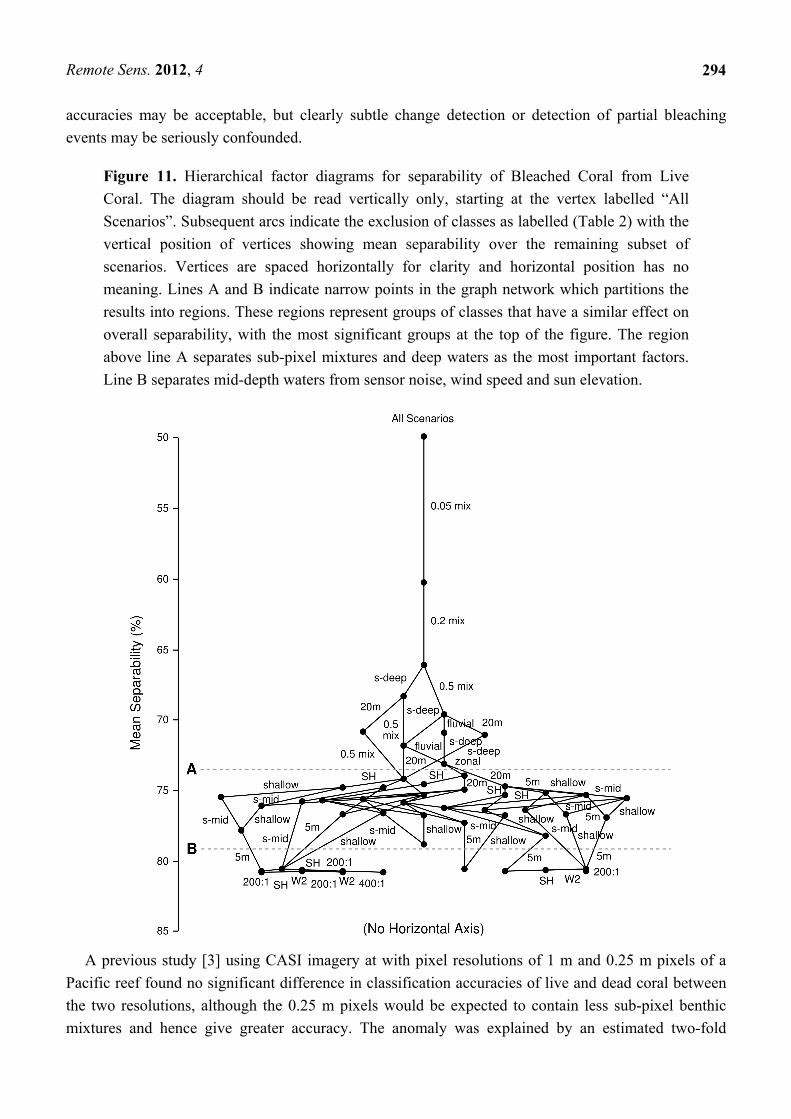
Moving downwards from the “All Scenarios” node, in all three Figures 11–13 there is an initial

large jump in overall accuracy attained by exclusion of all scenarios including the 0.05 benthic mixture

proportion followed by the 0.2 and 0.5 cover proportions, although for Bleached Coral and Dead Coral

exclusion of the 0.5 cover proportion class competes with 20 m depth and Deep multiple-depth class

(Figures 11 and 12). This indicates that attempting to discriminate sub-pixel proportions of the benthic

types was by far the biggest overall confounding factor for accuracy across the entire analysis. Any

level of sub-pixel mixing, reduced overall separability to below 73%, and even to below 60% for Live

Coral vs. Macroalgae. These results imply that benthic types that are mixed at sub-pixel scales will be

subject to a potential error in cover estimate of around one third (i.e., ~30%) of the areal extent of the

type to be detected. This potential error rises to one half (~50%) for benthic types in sub-pixel

proportions less than 0.2. This level of error is an upper limit and for some applications these


294

accuracies may be acceptable, but clearly subtle change detection or detection of partial bleaching

events may be seriously confounded.

Figure 11. Hierarchical factor diagrams for separability of Bleached Coral from Live

Coral. The diagram should be read vertically only, starting at the vertex labelled “All

Scenarios”. Subsequent arcs indicate the exclusion of classes as labelled (Table 2) with the

vertical position of vertices showing mean separability over the remaining subset of

scenarios. Vertices are spaced horizontally for clarity and horizontal position has no

meaning. Lines A and B indicate narrow points in the graph network which partitions the

results into regions. These regions represent groups of classes that have a similar effect on

overall separability, with the most significant groups at the top of the figure. The region

above line A separates sub-pixel mixtures and deep waters as the most important factors.

Line B separates mid-depth waters from sensor noise, wind speed and sun elevation.

A previous study [3] using CASI imagery at with pixel resolutions of 1 m and 0.25 m pixels of a

Pacific reef found no significant difference in classification accuracies of live and dead coral between

the two resolutions, although the 0.25 m pixels would be expected to contain less sub-pixel benthic

mixtures and hence give greater accuracy. The anomaly was explained by an estimated two-fold


295

increased environmental noise level in the higher resolution imagery, but in the results presented here

an SNR increase did not compensate for any level of sub-pixel mixing. However, firstly, the

interaction of benthic spatial distributions and pixel size was not assessed in [3], so it may not be true

that the 0.25 pixels were less mixed. Secondly, the higher resolution imagery had a lower spectral

resolution, 6 bands at 0.25 m vs. 10 bands at 1 m, and thirdly, the model presented here has a far higher

diversity of coral reflectance (Table 2) whereas the area surveyed in [3] was dominated by only two

genera (Porites and Pocillopora). These multiple qualifying factors illustrate the difficulty of making

general inferences from image-based studies.

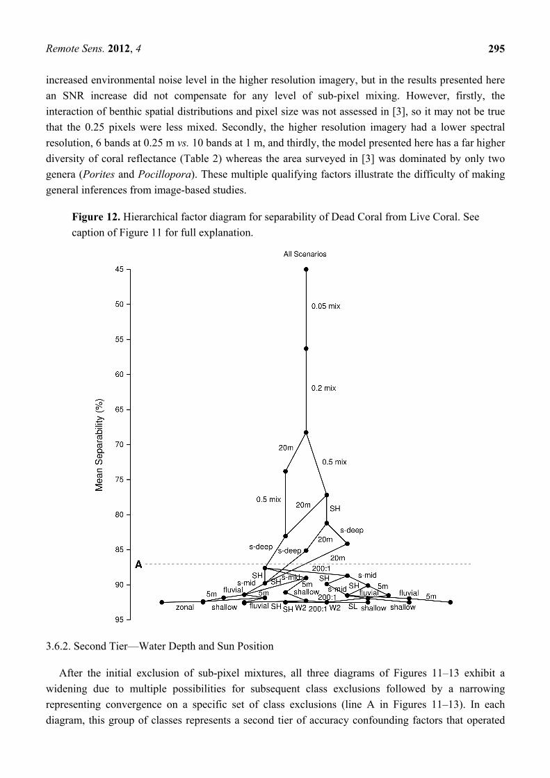
Figure 12. Hierarchical factor diagram for separability of Dead Coral from Live Coral. See

caption of Figure 11 for full explanation.

3.6.2. Second Tier—Water Depth and Sun Position

After the initial exclusion of sub-pixel mixtures, all three diagrams of Figures 11–13 exhibit a

widening due to multiple possibilities for subsequent class exclusions followed by a narrowing

representing convergence on a specific set of class exclusions (line A in Figures 11–13). In each

diagram, this group of classes represents a second tier of accuracy confounding factors that operated


296

after sub-pixel proportions had been excluded. A water depth of greater than 5 m was the most

significant confounding factor across all three graphs at this stage with almost all scenarios containing

the 20 m and the Shallow-Deep classes removed from the analysis by this point. Additionally,

differences among the benthic types start to emerge with many exclusions of high sun elevation for

Dead Coral and Macroalgae vs. the exclusion of the Fluvial IOP class from a large subsection of the

Bleached Coral diagram. Overall therefore, deep water was the next most significant confounding

factor for benthic class discrimination after sub-pixel proportions, followed by high sun position.

Reasonable water clarity was also important for detecting bleached coral at this accuracy level.

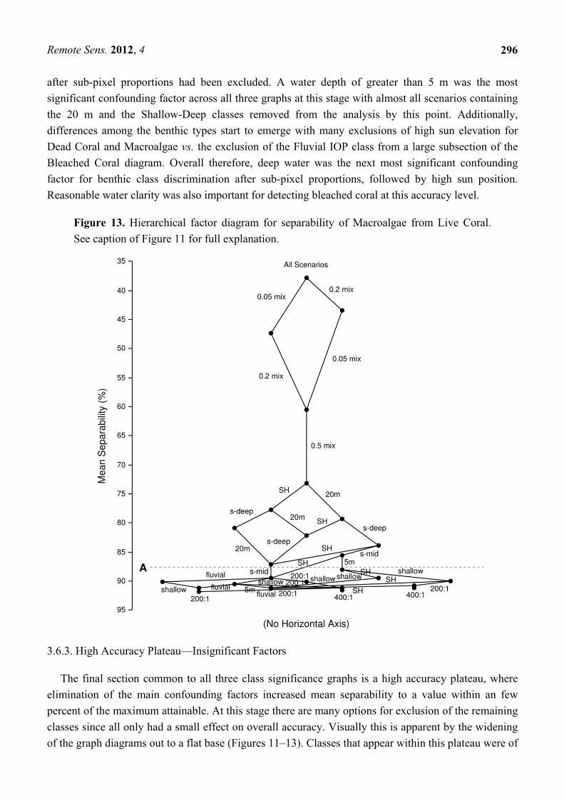
Figure 13. Hierarchical factor diagram for separability of Macroalgae from Live Coral.

See caption of Figure 11 for full explanation.

3.6.3. High Accuracy Plateau—Insignificant Factors

The final section common to all three class significance graphs is a high accuracy plateau, where

elimination of the main confounding factors increased mean separability to a value within an few

percent of the maximum attainable. At this stage there are many options for exclusion of the remaining

classes since all only had a small effect on overall accuracy. Visually this is apparent by the widening

of the graph diagrams out to a flat base (Figures 11–13). Classes that appear within this plateau were of


297

very little relative significance within the sensitivity analysis as a whole. For all three benthic types

excluded factors at this stage typically included the sensor SNR classes, wind speed classes and almost

all IOP classes, for clarity Figures 11–13 do not include all of these arcs and vertices. The Bleached

Coral graph is notable in that there is a clear intermediate step to high accuracy where remaining depth

classes except 0.5 m were excluded (line B in Figure 11). This indicates that any water depth greater

than 0.5 m was a confounding factor for detecting bleaching. The same effect is present but less

pronounced for Dead Coral and Macroalgae (Figures 12 and 13).

In the Bleached Coral diagram (Figure 11) there is a division into two subsections where in one case

the Fluvial IOP class was excluded and in the other it was retained. The division occurs at the point

where line A intersects the graph and persists to the high separability plateau, where the group of four

vertices on the left still contains the Fluvial IOP class but the three on the right do not. This illustrates

the interaction between water clarity and depth, as large depths were excluded low water clarity

became increasingly insignificant. Note however that the trade-off is highly unbalanced since the

graph construction implies that at almost every step excluding a depth class is twice as effective as

excluding an IOP class. This is consistent with the charts in Figures 8 and 9, which illustrate IOP class

only had a large effect on separability in the 20 m and Shallow-Deep classes.

The overall structure of the hierarchical graphs and subsequent conclusions are dependent on the

design of the sensitivity analysis class structure and the methodology of graph construction. However,

the class structure was designed to represent scenarios encountered in practical reef remote sensing

contexts. The major patterns in the results are fairly clear and consistent between the detailed analysis

(Figures 8 and 9) and the hierarchical summary (Figures 11–13) and can be further qualitatively

summarised as a single ranked list of confounding factors for benthic remote sensing, Table 6.

Table 6. Overall list of confounding factors for accuracy of benthic type separability

ordered by significance (based on the structure of the experiment design presented here).

(1) Detecting proportions less than 100% of any benthic type.

(2) Water depth > 5m.

(3) Fluvial variation in IOPs when detecting bleaching.

(4) High sun elevation (zenith angle 15° vs. 45°).

(5) Water depth > 0.5 m when detecting bleaching (less important for dead coral or macroalgae).

(6) Sensor SNR, wind speed and other IOP variations are overall not very significant factors.

4. Conclusions

One of the aims of this study has been to demonstrate a generic method for analysing a remote

sensing system in terms of individual environmental and sensor components. The aim of this method is

to be able to distinguish between environmentally limited objectives, where accuracy cannot benefit

from improved sensor design, and sensor-limited objectives, where specific sensor design

improvements will be effective and their effect on accuracy can be quantitatively predicted. Although

this paper has concentrated on benthic class separability, it is straightforward to turn the analysis

around and instead, for example, consider the capability to recover bathymetry or IOP class under

benthic class variation.


298

Within the scope of the experimental design presented here, the relative importance of several key

environmental and sensor design factors in accurately discriminating benthic classes in remotely

sensed image data has been established. For the benthic types considered here, sub-pixel quantification

was the most challenging objective. While previous modelling studies have not quantified the effect of

benthic class confusion across depths, this work has demonstrated that while depth itself is a serious

confounding factor for benthic remote sensing, depth variation introduces further spectral confusion

even for shallow waters (<2 m). That is, the fact that we do not know a priori exactly what depth a

pixel represents is a separate source of confusion than the fact that increasing depth attenuates the

reflected light. Overall, water column IOP spatial variation found in reef systems does little to

confound benthic class separability. This result supports the application of the latest techniques that

aim to extract both water properties and benthic class from optical data [19]. While most environmental

factors cannot be controlled by investigators, our model framework provides a method for determining

optimal conditions for those that can. This is demonstrated by the highlighting of sun elevation at

image acquisition as an important factor in the hierarchy of confounding factors (Table 6). An efficient

software implementation of the method could therefore be a useful planning tool for remote sensing

campaigns.

Overall, most modelled scenarios were environmentally limited, with sensor SNR limitation only

becoming significant under ideal environmental conditions of low wind speed and low sun elevation

and for certain benthic classes. However, sub-pixel mixing can be interpreted indirectly as a sensor

characteristic through being a function of spatial resolution. Since sub-pixel mixing was an

overwhelming confounding factor in the analysis and sensor SNR was not, it may be that current

airborne sensors would benefit in trading SNR for higher spatial resolution in reef applications.

Identifying the optimal spatial resolution will require an analysis of benthic spatial distributions on

reefs, but even a qualitative assessment based on experience of the scales of heterogeneity in reef

environments implies that in general resolutions below 1 m2 are required. Importantly, if future

predictions of decline of live coral cover on reefs are borne out, the difficulty in monitoring these

ecosystems by remote sensing will only increase. While bleached coral was the most robustly

discriminated benthic class under the range of conditions modelled, since bleaching events occur on

relatively short time scales of days to weeks the practical advantage of this detectability may

outweighed by the temporal resolution offered by satellite over-flight times, or the need to plan

airborne surveys.

For high spatial resolutions, water column effects causing lateral spectral mixing must also be

considered, i.e., the water column “point spread function” [24], plus effects due to benthic 3-dimensional

canopy structure. These effects cannot be assessed with the plane-parallel radiative transfer model used

here and so will require new modelling algorithms [31]. For satellite-borne sensors atmospheric effects

will also be a significant factor that will affect the balance of sensor SNR and spatial resolution. In this

study we have neglected to consider differing sensor spectral resolutions as this has been addressed

before [6,7]. However this design factor will also be trade-off with SNR and spatial resolution and

cannot be treated in isolation from these or the environmental factors included here. Future work will

extend the model framework presented here to incorporate all the above-discussed factors, the primary

difficulty being to make the resulting multi-factor analysis computationally tractable. Nevertheless,


299

developing such a generic modelling framework would seem a highly cost-effective method for

improving understanding of remote sensing systems and advising on future practical directions.

With respect to the estimated separabilities presented here, as the current model is simplified in

certain respects and excludes an atmospheric component, these will be upper bounds on what will be

achievable in practice. Although it could be argued that non-linear analysis techniques such as

successive approximation models, look-up tables or neural networks [17,18,46,47] may perform better

under certain circumstances than the linear separability measure used here, the significant spectral

space class overlap that must be present for some factor combinations will confound any analytical

method. Similarly, any pre-processing steps that only manipulate individual pixel spectra, such as

removing water column effects by depth invariant indices [22,44] will have little impact on

separability as identical spectra remain identical after transformation. Conversely, techniques that

incorporate additional data sources such a sonar bathymetry [48], do in theory add information and

could resolve cases of spectral confusion. Therefore, while there are definite environmental limitations

to what can be achieved by any sensor or algorithm, the future potential to overcome these limitations

resides in data synthesis across multiple sources.

Acknowledgements

This project was funded by the World Bank/GEF Coral Reef Targeted Research and Capacity

Building Program with additional contributions from the UK Natural Environment Research Council

(grants NER/Z/S/2001/01029 and NE/C513626/1) and the Australian Research Council Discovery

Project (DP0663893. Innovative Coral Reef Mapping) to Phinn and Mumby. The authors are grateful

for the assistance of the University of the South Pacific and the South Pacific Geosciences Committee.

The manuscript was improved thanks to the comments of Edward Smith.

References

1. Elvidge, C.D.; Dietz, J.B.; Berklemans, R.; Andréfouët, S.; Skirving, W.; Strong, A.E.; Tuttle, B.T.;

Satellite observation of Keppel Islands (Great Barrier Reef) 2002 coral bleaching using IKONOS

data. Coral Reefs 2004, 23, 123-132.

2. Mumby, P.J.; Chisholm, J.R.M.; Clark, C.D.; Hedley, J.D.; Jaubert, J. A bird’s eye view of the

health of coral reefs. Nature 2001, 413, 36.

3. Mumby, P.J.; Hedley, J.D.; Chisholm, J.R.M.; Clark, C.D.; Ripley, H.; Jaubert, J. The cover of

living and dead corals from airborne remote sensing. Coral Reefs 2004, 23, 171-183.

4. Hedley, J.D.; Mumby, P.J. Biological and remote sensing perspectives of pigmentation in coral

reef organisms. Adv. Mar. Biol. 2002, 43, 277-317.

5. Lesser, M.P.; Mobley, C.D. Bathymetry, water optical properties, and benthic classification of

coral reefs using hyperspectral remote sensing imagery. Coral Reefs 2007, 26, 819-829.

6. Hochberg, E.J.; Atkinson, M.J.; Andréfouët, S. Spectral reflectance of coral reef bottom types

worldwide and implications for coral reef remote sensing. Remote Sens. Environ. 2003, 85,

159-173.

7. Hochberg, E.J.; Atkinson, M.J. Capabilities of remote sensors to classify coral, algae and sand as

pure and mixed spectra. Remote Sens. Environ. 2003, 85, 174-189.


300

8. Karpouzli, E.; Malthus, T.J.; Place, C.J. Hyperspectral discrimination of coral reef benthic

communities in the western Caribbean. Coral Reefs 2004, 23, 141-151.

9. Kutser, T.; Dekker, A.G.; Skirving, W. Modeling spectral discrimination of Great Barrier Reef

benthic communities by remote sensing instruments. Limnol. Oceanogr. 2003, 48, 497-510.

10. Lubin, D.; Li, W.; Dustan, P.; Mazel, C.H.; Stamnes, K. Spectral Signatures of coral reefs:

Features from space. Remote Sens. Environ. 2001, 75, 127-137.

11. Malthus, T.; Mumby, P.J. Remote sensing of the coastal zone: An overview and priorities for

future research. Int. J. Remote Sens. 2003, 24, 2805-2815.

12. Phinn, S.R.; Dekker, A.G.; Brando, V.E.; Roelfsema, C.M. Mapping water quality and substrate

cover in optically complex coastal and reef waters: An integrated approach. Mar. Pollut. Bull.

2005, 51, 459-469.

13. Hedley, J.D.; Mumby, P.J.; Joyce, K.E.; Phinn, S.R. Spectral unmixing of coral reef benthos under

ideal conditions. Coral Reefs 2004, 23, 60-73.

14. Hedley, J.D.; Mumby, P.J. A remote sensing method for resolving depth and subpixel

composition of aquatic benthos. Limnol. Oceanogr. 2003, 48, 480-488.

15. Lee, Z.P.; Carder, K.L.; Mobley, C.D.; Steward, R.G.; Patch, J.S. Hyperspectral remote sensing

for shallow waters, 1. A semi-analytical model. Appl. Opt. 1998, 37, 6329-6338.

16. Lee, Z.P.; Carder, K.L.; Mobley, C.D.; Steward, R.G.; Patch, J.S. Hyperspectral remote sensing

for shallow waters, 2. Deriving bottom depths and water properties by optimization. Appl. Opt.

1999, 38, 3831-3843.

17. Lee, Z.; Carder, K.L.; Chen, R.F.; Peacock, T.G. Properties of the water column and bottom

derived from Airborne Visible Infrared Imaging Spectrometer (AVIRIS) data. J. Geophys. Res.

2001, 106, 11639-11651.

18. Mobley, C.D.; Sundman, L.K.; Davis, C.O.; Bowles, J.H.; Downes, T.V.; Leathers, R.A.;

Montes, M.J.; Bisset, W.P.; Kohler, D.D.R.; Reid, R.P.; Louchard, A.M.; Gleason, A.

Interpretation of hyperspectral remote-sensing imagery by spectrum matching and look-up tables.

Appl. Opt. 2005, 44, 3576-3592.

19. Brando, V.E.; Anstee, J.M.; Wettle, M.; Dekker, A.G.; Phinn, S.R.; Roelfsema, C. A physics

based retrieval and quality assessment of bathymetry from suboptimal hyperspectral data. Remote

Sens. Environ. 2009, 113, 755-770.

20. Hedley, J.D.; Roelfsema, C.M.; Phinn, S.R. Efficient radiative transfer model inversion for remote

sensing applications. Remote Sens. Environ. 2009, 113, 2527-2532.

21. Dekker, A.G.; Phinn, S.R.; Anstee J.; Bissett P.; Brando V.E.; Casey B.; Fearns P.; Hedley, J.;

Klonowski W.; Lee, Z.P.; Lynch, M.; Lyons, M.; Mobley, C.; Roelfsema, C. Intercomparison of

shallow water bathymetry, hydro-optics, and benthos mapping techniques in Australian and

Caribbean coastal environments. Limnol. Oceanogr. Methods 2011, 9, 396-425.

22. Green, E.P.; Mumby, P.J.; Edwards A.J.; Clark, C.D. Remote Sensing Handbook for Tropical

Coastal Management; UNESCO: Paris, France, 2000.

23. Mobley, C.D. Thematic mapping. In Ocean Optics Web Book; 2012. Available online:

http://www.oceanopticsbook.info/view/remote_sensing/level_2/thematic_mapping (accessed on

20 January 2012).


301

24. Mobley, C.D.; Sundman, L.K. Effects of optically shallow waters on upwelling radiances:

Inhomogeneous and sloping bottoms. Limnol. Oceanogr. 2003, 48, 329-336.

25. Grant, R.H.; Hiesler, G.M.; Gao, W. Photosynthetically-active radiation: Sky radiance

distributions under clear and overcast conditions. Agric. For. Meteorol. 1996, 82, 267-292.

26. Cox, C.; Munk, W. Statistics of the sea surface derived from sun glitter. J. Mar. Res. 1954, 13,

198-227.

27. Mobley, C.D. Light and Water; Academic Press: San Diego, CA, USA, 1994.

28. Mather, P.M. Computer Processing of Remotely-Sensed Images, 2nd ed.; Wiley: New York, NY,

USA, 1999.

29. Lucas, R.; Rowlands, A.; Niemann, O.; Merton, R.N. Hyperspectral sensors and applications. In

Advanced Image Processing Techniques for Remote Sensed Hyperspectral Data; Varshney, P.K.,

Arora, M.J., Eds.; Springer-Verlag: New York, NY, USA, 2004; pp. 11-49.

30. Roelfsema, C.M.; Marshall, J.; Hochberg, E.; Phinn, S.; Goldizen, A.; Joyce, K. Underwater

Spectrometer System 2004 (UWSS04); Centre for Remote Sensing and Spatial Information

Science, University of Queensland: Brisbane, QLD, Australia, 2006.

31. Hedley, J. A three-dimensional radiative transfer model for shallow water environments. Opt.

Express 2008, 16, 21887-21902.

32. Mobley, C.D.; Sundman, L.K. Hydrolight 4.1 Users’ Guide; Sequoia Scientific Inc.: Redmond,

WA, USA, 2000.

33. Hedley, J.D.; Harborne, A.R.; Mumby, P.J. Simple and robust removal of sun glint for mapping

shallow water benthos. Int. J. Remote Sens. 2005, 26, 2107-2112.

34. Mueller, J.L. Ocean Optics Protocols for Satellite Ocean Color Sensor Validation; NASA/TM

2003-211621/Rev 4-Vol IV (Erratum 1); 2003.

35. Smith, R.C.; Baker, K.S. Optical properties of the clearest natural waters (200–800 nm). Appl.

Opt. 2001, 20, 177-184.

36. Boss, E.; Pegau, W.S. Relationship of light scattering at an angle in the backward direction to the

backscattering coefficient. Appl. Opt. 2001, 40, 5503-5507.

37. Mobley, C.D.; Sundman, L.K.; Boss, E. Phase function effects on oceanic light fields. Appl. Opt.

2002, 41, 1035-1050.

38. Karpouzli, E.; Malthus, T.; Place, C.; Mitchell Chui, A.; Ines Garcia, M.; Mair, J. Underwater

light characterisation for correction of remotely sensed images. Int. J. Remote Sens. 2003, 24,

2683-2702.

39. Tabachnick, B.G.; Fidell, L.S. Using Multivariate Statistics, 4th ed.; Allyn and Bacon: London,

UK, 2001.

40. Ma, Z.; Redmond, R.L. Tau coefficients for accuracy assessment of classification of remotely

sensed data. Photogramm. Eng. Remote Sensing 1995, 61, 435-439.

41. Sokal, R.R.; Rohlf, F.J. Biometry, 3rd ed.; Freeman: San Francisco, CA, USA, 1995.

42. Christofides, N. Graph theory. An algorithmic approach. Academic Press, London, UK, 1975.

43. Leiper, I.A.; Siebeck, U.E.; Marshall, N.J.; Phinn, S.R. Coral health monitoring: Linking coral

colour and remote sensing techniques. Can. J. Remote Sensing 2009, 35, 276-286.

44. Lyzenga, D.R. Passive remote sensing techniques for mapping water depth and bottom features.

Appl. Opt. 1978, 17, 379-383.


302

45. Wettle, M.; Brando, V.E. SAMBUCA: Semi-Analytical Model for Bathymetry, Un-Mixing, and

Concentration Assessment; CSIRO Land and Water Science Report 22/06; CSIRO: Canberra,

ACT, Australia, 2006.

46. Calvo, S.; Ciraolo, G.; La Loggia, G. Monitoring Posidonia oceanica meadows in a Mediterranean

coastal lagoon (Stagnone, Italy) by means of neural network and ISODATA classification

methods. Int. J. Remote Sens. 2003, 24, 2703-2716.

47. Ceyhun, Ö.; Yalcin, A. Remote sensing of water depths in shallow waters via artificial neural

networks. Estuar. Coast. Shelf Sci. 2010, 89, 89-96.

48. Bejerano, S.; Mumby, P.J.; Hedley, J.D.; Sotheran, I. Combining optical and acoustic data to

enhance the detection of Caribbean fore-reef habitats. Remote Sens. Environ. 2010, 114, 2768-2778.

© 2012 by the authors; licensee MDPI, Basel, Switzerland. This article is an open access article

distributed under the terms and conditions of the Creative Commons Attribution license

(http://creativecommons.org/licenses/by/3.0/).

Documents

Remotesensing-04-00271_Environmental and Sensor Limitations in Optical Remote Sensing of Coral Reef