Air Pollutant Exposure Associated with

Distributed Electricity Generation

Final Report

Contract No. 01-341

Prepared for the

California Air Resources Board

and the California Environmental Protection Agency

Prepared by

Garvin A. Heath, Abigail S. Hoats and William W Nazaroff

Department of Civil and Environmental Engineering

631 Davis Hall

University of California

Berkeley, CA 94720-1710

April 2003

Disclaimer The statements and conclusions in this Report are those of the contractor and not necessarily those of the California Air Resources Board. The mention of commercial products, their source, or their use in connection with material reported herein is not to be construed as actual or implied endorsement of such products.

i

Acknowledgements Professor Catherine Koshland served as an advisor for this research. Julian Marshall provided insightful feedback at many stages of the research. We acknowledge their contributions with gratitude. In addition to the financial support of the California Air Resources Board, we acknowledge the support of the University of California’s Toxic Substances Research and Training Program and the U.S. Environmental Protection Agency’s Science to Achieve Results graduate fellowship, which provided support for Garvin Heath and Abby Hoats during this research. This report was submitted in fulfillment of Contract No. 01-341, Air Pollutant Exposure Associated with Distributed Generation, by the University of California under the sponsorship of California Air Resources Board. Work was completed as of April 4, 2003.

ii

Table of Contents Disclaimer ........................................................................................................................... i Acknowledgements ........................................................................................................... ii Table of Contents ............................................................................................................. iii List of Figures.................................................................................................................... v List of Tables ................................................................................................................... vii Abstract........................................................................................................................... viii Executive Summary ......................................................................................................... ix I. Introduction........................................................................................................... 1 II. Methods................................................................................................................ 11

II.A Electricity Generation Units: Location and Background Information......... 12 II.B Pollutant Selection ....................................................................................... 18 II.C Modeling Tools and Input Data ................................................................... 18

II.C.1 Gaussian Plume Model .......................................................................... 18 II.C.1.a Gaussian Plume Model for Conserved Pollutants ............................ 18 II.C.1.b Gaussian Plume Model for Decaying Pollutants .............................. 20

II.C.2 Meteorological Parameters .................................................................... 21 II.C.2.a Mixing Height................................................................................... 21 II.C.2.b Wind Speed and Direction ................................................................ 21 II.C.2.c Atmospheric Stability Class.............................................................. 24

II.C.3 Population Parameters ........................................................................... 26 II.C.4 Power Plant and Pollutant Data ............................................................. 28

II.C.4.a Power Plant Data............................................................................... 28 II.C.4.b Pollutant Data.................................................................................... 32

II.D Modeled Parameters..................................................................................... 34 II.D.1 Hazard Index.......................................................................................... 34 II.D.2 Intake Fraction....................................................................................... 35

II.D.2.a Intake Fraction of Conserved Pollutants .......................................... 36 II.D.2.b Intake Fraction for a Decaying Pollutant ......................................... 37

II.D.3 Intake Factor.......................................................................................... 37 III. Results and Discussion........................................................................................ 38

III.A Hazard Ranking Results............................................................................... 38 III.B Intake Fraction Results................................................................................ 40

III.B.1 Conserved Pollutants Results................................................................. 40 III.B.2 Key Factors Governing Intake Fraction for Conserved Pollutants ....... 44 III.B.3 Decaying Pollutant Results .................................................................... 47 III.B.4 Cumulative Intake Fraction ................................................................... 49 III.B.5 Comparison to Previously Published Research ..................................... 55 III.B.6 Refined Analysis of Meteorological and Population Density Data ....... 56

III.C Intake Factor Results................................................................................... 58 III.D Summary of Results..................................................................................... 65

IV. Conclusions .......................................................................................................... 65

iii

V. Recommendations ............................................................................................... 67 VI. References ............................................................................................................ 70 VII. Glossary of Terms, Abbreviations, Units of Measure and Symbols............... 75 Appendix .......................................................................................................................... 81 A.I. Methods................................................................................................................ 81

A.I.A Gaussian Plume Model for Conserved Pollutants ....................................... 81 A.I.B Meteorological Parameters .......................................................................... 82

A.I.B.1 Mixing Height........................................................................................ 82 A.I.B.2 Wind Speed and Direction ..................................................................... 82 A.I.B.3 Atmospheric Stability Class................................................................... 82

A.I.C Population Parameters ................................................................................. 83 A.I.D Intake Fraction Calculation ......................................................................... 87 A.I.E Environmental Justice Analysis................................................................... 87

A.II. Results and Discussion........................................................................................ 88 A.II.A Annual-Average Intake Fraction ................................................................. 88 A.II.B Population Distribution Analysis................................................................. 90 A.II.C Annual-Average Intake Fraction Comparison ............................................ 94 A.II.D Environmental Justice Analysis................................................................... 97

A.III. Conclusions .......................................................................................................... 99

iv

List of Figures Figure 1. Percentage of total U.S. emissions released by fossil-fuel electricity generation

units and other sources in 1999................................................................................... 2 Figure 2. Fraction of 2001 California electricity production (GWh) by fuel-type, with

imports allocated to fuel-type category....................................................................... 4 Figure 3. Map of locations of Morro Bay and El Segundo central stations. Photographs

of the facilities are displayed to the left, with arrows indicating to which location they belong................................................................................................................ 14

Figure 4. Map of locations of two of the three microturbine cases. A picture of a microturbine is provided to the left of the map (Capstone, 2002). A microturbine was also modeled at the site of the Morro Bay central station (see Figure 3). ......... 17

Figure 5. Wind direction histogram for Los Angeles, CA, based on typical meteorological year data (TMY2) (NREL, 1995). ............................................................................ 23

Figure 6. Wind direction histogram for Santa Maria, CA, based on typical meteorological year data (TMY2) (NREL, 1995). ................................................... 23

Figure 7A, B and C. Population density (people/km2) as a function of downwind distance for each of the three locations of electricity generation units: A) Morro Bay; B) El Segundo; and C) Downtown LA............................................................................... 27

Figure 8A, B, C, D and E. Conserved pollutant iFs by stability class for A) Morro Bay Power Plant; B) El Segundo Generating Station; C) a microturbine at the site of Morro Bay Power Plant; D) a microturbine at the site of El Segundo Generating Station; and E) a microturbine in downtown Los Angeles (10 km inland). These values have been adjusted for conditions leading to zero intake when appropriate. 41

Figure 9. Annual-average iFs for a conserved pollutant for all cases, adjusted for conditions leading to zero intake, as appropriate...................................................... 43

Figure 10. iF results from sequentially switching certain, key parameters, starting from the El Segundo central station case and moving to the DG at Morro Bay case for conserved pollutants. These cases were adjusted for conditions leading to zero intake, as appropriate. ............................................................................................... 46

Figure 11. Annual-average iFs for a conserved pollutant and HCHO for all cases, adjusted for conditions leading to zero intake, as appropriate.................................. 48

Figure 12. Conserved pollutant iFs as a function of downwind distance for stability class C (slightly unstable) for El Segundo and a microturbine (“DG”) located at the same site, varying downwind population density from the actual to a distance-weighted average population density. ...................................................................................... 50

Figure 13. Conserved pollutant iFs as a function of downwind distance for stability class D (neutral) for El Segundo and a microturbine (“DG”) located at the same site, varying downwind population density from the actual to a distance-weighted average population density. ...................................................................................... 51

Figure 14. Conserved pollutant iFs as a function of downwind distance for stability class F (moderately stable) for El Segundo and a microturbine (“DG”) located at the same site, varying downwind population density from the actual to a distance-weighted average population density. ...................................................................................... 52

Figure 15. HCHO iFs as a function of downwind distance for stability class C (slightly unstable) for El Segundo and a microturbine (“DG”) located at the same site,

v

varying downwind population density from the actual to a distance-weighted average population density. ...................................................................................... 54

Figure 16. Comparison of annual-average intake fraction between the original, modal wind direction model and the refined model for a conserved pollutant.. ................. 57

Figure 17. Intake factors for primary PM2.5 emissions from two existing and two new central stations and three existing DG cases (i.e., DG installed before the CARB 2003 DG emission standard)..................................................................................... 61

Figure 18. Intake factors for primary HCHO emissions from two existing and two new central stations and three existing DG cases (i.e., DG installed before the CARB 2003 DG emission standard)..................................................................................... 62

Figure 19. Estimate of PM2.5 emission factors necessary for newly installed DG to equal the iFacs of existing or new central stations............................................................. 63

Figure 20. Estimate of HCHO emission factors necessary for newly installed DG to equal the iFacs of existing or new central stations. .................................................. 64

Figure A1. Electricity generation locations with points at 0.5 km intervals radiating in

twelve directions ....................................................................................................85 Figure A2. Zoom in on El Segundo and downtown LA with points at 0.5 km intervals

radiating in twelve directions.................................................................................86 Figure A3. Annual-average intake fractions for a conserved pollutant using the refined

model......................................................................................................................89 Figure A4. Population data inputs for the Morro Bay modal wind direction ...................91 Figure A5. Population data inputs for the El Segundo modal wind direction ..................92 Figure A6. Population data inputs for the downtown LA modal wind direction .............93 Figure A7. Comparison of annual-average intake fraction between the original, modal

wind direction model and the refined model for a conserved pollutant ................95 Figure A8. Comparison between three modeling scenarios of annual-average intake

fraction for a conserved pollutant ..........................................................................96 Figure A9. Environmental justice analysis .......................................................................98

vi

List of Tables Table 1. Selected 2000 emission inventory data (tons per day, annual average) for

California. .................................................................................................................3 Table 2. Typical characteristics of the central station and distributed generation (DG)

paradigms of electricity generation relevant to air quality and inhalation exposure.. .................................................................................................................6

Table 3. Efficiencies and emissions factors of selected distributed generation technologies.. ...........................................................................................................8

Table 4. Selected data relevant to air quality for El Segundo and Morro Bay central stations. ..................................................................................................................13

Table 5. Modeling characteristics of the three microturbine cases relevant to air quality. ...................................................................................................................16

Table 6. Summary of meteorological data for each case. .................................................25 Table 7. Emission factors used in modeling the three central station cases (Morro Bay,

El Segundo and new central stations) and existing microturbines. .......................31 Table 8. Total daytime rate constant for HCHO decay considering reaction with the

hydroxyl radical (OH) and photolysis....................................................................33 Table 9. Hazard ranking for Morro Bay and El Segundo central station plants and for

existing microturbines............................................................................................39 Table 10. Step that a given parameter was changed in moving from the case of El

Segundo central station to microturbine at Morro Bay. ........................................45 Table 11. Intake factors for the three central station cases (Morro Bay, El Segundo and

new central-station plants) and existing microturbines, as well as an estimate of emission factors for new microturbines necessary to equalize intake factors of central station technologies....................................................................................60

Table A1. Case study locations.........................................................................................84

vii

Abstract Private sector and governmental organizations recently have promoted the deployment of small-scale, distributed electricity generation (DG) technologies for their many benefits as compared to the traditional paradigm of large, centralized power plants. However, there is reason to caution against an unmitigated embrace of combustion-based DG. We conducted a series of case studies that combined air dispersion modeling and an exposure assessment. This investigation has revealed that the fraction of pollutant mass emitted that is inhaled by the downwind, exposed population (i.e., the intake fraction) can be more than an order-of-magnitude greater for natural gas-fired, microturbine DG technologies than for large, natural gas-burning, central-station power plants. This result is a consequence mainly of the closer proximity of DG sources to densely populated areas as compared to typical central stations. Considering uncontrolled emission factors for DG technologies (e.g., those installed before the 2003 California DG emission standard), the mass of pollutant inhaled normalized by the electricity delivered (i.e., the intake factor) can be up to four orders-of-magnitude greater for microturbines as compared to central stations. In order to equalize the exposure burden between DG and central station technologies, microturbine emission factors will need to be reduced to a range between the level of the cleanest, new central stations and two orders of magnitude below those levels, depending on the pollutant and siting. Continued research to refine our preliminary results could lead to an emissions target for DG sources so that they do not pose a greater public health burden than the current electricity generation system.

viii

Executive Summary Background

The electricity generation system in California is undergoing major changes. The electric industry is being restructured, retail markets are now open to competition, and new generation technologies are being developed. One important aspect of these changes is a shift from a heavy reliance on central-station power plants toward more distributed generation of electricity. Distributed generation (DG) is defined as “electrical generation close to the place of use” (SB1298). DG technologies vary enormously in their air quality significance, from zero-emissions solar and wind power to high-emitting diesel-powered generators. Because units are sized according to the local demand, even the high-emitting technologies may be sufficiently small to not require an air permit to operate. Yet, widespread use of distributed generation could lead to substantially increased pollutant emissions in close proximity to people. Consequently, there are legitimate concerns about the possible air quality impacts of a shift in electricity production from central power plants to distributed generation.

Senate Bill 1298 charged the California Air Resources Board (CARB) with the development of regulations for air pollutant emissions from distributed generation. The regulations developed thus far aim to equalize emissions per unit of electricity generated from DG technologies as compared to modern central power stations. However, one important aspect of a shift from centralized power generation to DG is the potential for closer proximity between emissions and people. Closer proximity can cause higher exposures, even if the pollutant mass emitted is unchanged. Methods

This study evaluates the potential for increased inhalation exposure to air pollutant emissions due to a paradigm shift in the scale of electricity generation, from central stations to distributed generation. We use case studies of real and hypothetical electricity generation units to represent the range of natural gas-fired, baseload electricity generation facilities in California today. Gaussian plume modeling across a range of typical meteorological conditions estimates the downwind concentrations of certain emitted pollutants within 100 km of the source. By combining these predictions with population data and breathing rates, we estimate the total population intake of a pollutant associated with a particular source. The intake fraction (iF) is defined to be the population intake divided by the mass emitted, or the fraction of emissions that are inhaled by the downwind population. This is an appropriate figure of merit for comparing the exposure potential of the two paradigms of electricity generation.

The intake fraction multiplied by a pollutant emission factor is termed the intake factor (iFac). This figure of merit represents the population intake normalized per unit of electricity delivered to the end user and incorporates the differences in efficiency, emission rates and line losses among technologies. The intake factor forms another basis of comparison between the cases of existing DG and central station technologies used in this study. We then use the intake factor to estimate what new DG emission factors should be so not to present a greater exposure burden than central stations.

ix

Results Our case-study approach provides important indications of the differences in

population exposure to air pollutants emitted from the two paradigms of electricity generation, as well as their underlying causes. We find that intake fractions differ by an order of magnitude or more between DG and central stations. The underlying reason for the considerable difference traces to two factors. First, the difference in stack heights (~5 m for DG and ~250-450 m for central stations) leads to much closer proximity of the emissions to people for DG technologies. Closer proximity yields higher exposure concentrations and, thus, greater intake. Second, population density of the likely siting locations for DG is much higher than for central station plants. Central station plants are commonly located in rural or industrial areas on the outskirts of population centers. Many DG units, on the other hand, are likely to be located in the downtown business district of major cities. Higher population density in close proximity to the source leads to a greater number of people exposed, which increases the intake fraction.

When normalized per unit of electricity delivered, the resulting intake factors are one to four orders-of-magnitude greater for the cases of existing, uncontrolled DG units as for the central stations considered in this study. Differences in emission factors compound the disparity in intake fraction to yield significantly greater population intake per unit of electricity delivered for existing DG units. In order to equalize the exposure burden of existing and new central stations, new DG technologies will have to emit at no greater rate than the cleanest, new central stations and in many cases at levels up to two orders-of-magnitude lower than those rates. Conclusions

While the specific results of this study reflect the particularities of the cases selected, the scale of the effects observed, the confirmation of the magnitude and trends of the results by an alternative assessment in the Appendix, and the elucidation of their underlying causes suggest that our broad findings may be true beyond the limits of the cases considered. Thus, this research has implications for air quality and energy policy.

The early concern of higher emission rates has been addressed in California for four pollutants; by 2007, DG emissions of those pollutants per unit electricity generated should be no greater than those from central stations. However, achieving parity in mass emission rates does not ensure equal air pollutant exposure impacts. In addition, the standard does not mandate limits on many other pollutants of concern. To be protective of public health, regulators should consider the potential for increased exposures to air pollutants emitted by combustion-based DG technologies, including those pollutants not currently regulated.

The exposure penalty revealed here can help define a new DG emissions target to equalize inhalation exposures and health impacts. To accomplish this goal, emission factors from DG technologies will have to be much better than from central stations, a goal that will take time to achieve. More research is needed to refine and substantiate our initial findings. In the meantime, regulators should consider increasing the promotion of ultralow-emitting technologies, such as fuel cells, or nonemitting technologies, such solar photovoltaics, to capture the many benefits of distributed generation without incurring the risks to public health concomittant with combustion-based technologies.

x

I. Introduction Electricity generation has major impacts on the environment at local, regional and

global scales. Fossil fuel-based generation is especially important for local and regional air quality. According to U.S. emission inventories, electricity generation contributes a significant fraction of national emissions of certain pollutants (Figure 1). The share of total emissions in California is lower (Table 1) due to tighter environmental regulations, fuel switching and a high percentage (slightly less than half) of non-emitting generation (CEC, 2001a). Nevertheless, electricity generation’s contribution to California’s statewide emissions from combustion-related activities remains substantial (Table 1).

A long history of concern about such emissions has led to significant improvements in the polluting characteristics of electricity generation across the nation. Both absolute and relative emissions have decreased significantly over the last few decades, especially in California (CEC, 2001a). For instance, the contribution of electricity generation to total statewide nitrogen oxides (NOx) emissions fell from 7% in 1980 to 2% in 1990 and then remained at 2% in 2000 despite a declining base of total emissions (Scheible, 2002). Multifaceted control programs involving cleaner fuels, improved combustion, emission control devices and process modifications are responsible for the improvements.

Electricity is generated by many technologies with different characteristics. California’s electricity generation units are diverse, both in fuel-type (Figure 2) and size. However, total electrical output and emissions are concentrated in the largest plants. Of approximately 1000 units, the 100 largest, with capacities of over 100 megawatts (MW) each, constitute nearly 75% of the total generating capacity in the state (CEC, 2001c). In addition, 46% of the total NOx emissions from electric utilities in California come from the ten largest fossil-fuel burning plants (CARB, 2000b). Thus, individual power plants can be large sources of air pollutants.

Combustion-based technologies are the subject of this analysis, because they are the source of almost all direct air pollutant emissions from electricity generation. 1 We will focus on units that burn natural gas. Natural gas is a popular fuel choice for existing and new capacity. Forty-five percent of electricity production and 53% of current capacity in California is provided in natural gas-fueled plants (CEC, 2001b and CEC, 2002c). Since 1999, 100% of licensing applications approved by the California Energy Commission (CEC) are for natural gas facilities, mainly combined cycle (CEC, 2002a).

For most of the past century, the United States has used a regulated monopoly model for ensuring reliable and adequate production of electricity at reasonable cost. Since the mid-1990’s, many state legislatures, including California’s, have significantly restructured the electric power industry within their jurisdictions. This restructuring has led to increased competition and has reduced central planning and large infrastructure investments. Parallel with this change have been advances in electric generation technology leading to a wave of new, smaller-scale generators on the market. Because of their size and proportional cost, smaller-scale technologies present a greater opportunity for private ownership of power production, heralding a shift towards more distributed generation of electricity. 1 Hydrogen sulfide emissions from geothermal plants provide the only major exception.

1

67

23

33

33

67

77

0 20 40 60 80 100

Sulfur Dioxide

NitrogenOxides

Toxics

Electricity Generation Other Sources

Figure 1. Percentage of total U.S. emissions released by fossil-fuel electricity generation units and other sources in 1999. [Toxics data source: EPA, 2002a; others: GAO, 2002]

2

Table 1. Selected 2000 emission inventory data (tons per day, annual average) for California.

Emission Source ROGa COb NOxc SO2

d PM10e

Electric utilities 4.3 32 46 3.8 5Cogeneration 4.1 38 33 2.1 3.6Total electric utilities plus cogeneration 8.4 70 79 5.9 8.6

Total stationary fuel combustion 41 295 494 57 43

Total statewide 3311 21035 3591 333 2403a ROG = reactive organic gases b CO = carbon monoxidec NOx = oxides of nitrogen d SO2 = sulfur dioxidee PM10 = particulate matter less than 10 µm in diameterSource: CARB, 2000a.

3

Natural Gas

OilCoal

Nuclear

Hydro, large

Geothermal

Other Renewables

Figure 2. Fraction of 2001 California electricity production (GWh) by fuel-type, with imports allocated to fuel-type category. Source: CEC, 2001b

4

Formally, distributed generation, or DG, can be defined as, “electric power generation within the distribution network or on the customer side of the meter” (Ackerman et al., 2001). Operationally, any electricity generated “near the place of use” is known as distributed generation (SB 1298, 1999); this is the definition used in this report since it is codified in California law and regulation. The alternative paradigm of electricity generation, typified by 1,000-megawatt (MW) or greater utility-owned power plants, mostly constructed in the middle of the last century, is referred to as “central station.” California has twelve major central stations, each having a generating capacity of 1,000 MW or greater (CEC, 2001c).

Major central station power plants are classic “point sources” for air quality engineering and regulation. They provide power to the electrical grid to be used anywhere that transmission lines can connect them to a demand. Smaller central station power plants (e.g., less than 300 MW) are more numerous, but on average the emissions and power generation from the electricity-generating system is concentrated toward the largest central stations (CARB, 2000b). 2 Size (or capacity) of DG plants is actually not limited by the above definitions, although in practice, entities generating electricity for their own needs seldom produce more than 50 MW. More typically, DG units have less than 1 MW capacity. Table 2 further summarizes some of the differences between DG and central stations that are especially relevant to human exposures to air pollutants.

2 While total mass emissions are concentrated in the larger facilities, smaller generators can sometimes have much higher emissions on a per kilowatt-hour basis. This can be important for local exposures and has implications for regulatory approaches to deal with high emitters.

5

Table 2. Typical characteristics of the central station and distributed generation (DG) paradigms of electricity generation relevant to air quality and inhalation exposure.

Electricity Generation Paradigm

Capacity (MW) Location

Effective Stack Height (m)a

Applicable Emission Regulations

a Effective stack height is discussed in Section II.C.4.a; for DG, the range is defined by placement of the unit either on the ground or on the top of a building. Central station effective stack heights are calculated based on the typical assessment of plume rise (owing to exit velocity and temperature) plus physical stack height.

DG Typ. < 1 - Suburban- Urban None yet1 - 50

Central Station Typ. > 300 50 – 450 Many- Rural- Suburban- Coastal urban

6

Distributed generation can include both old and new technologies, which can use a range of primary energy sources, including fossil fuel combustion and renewable resources. However, in some circles, DG refers only to small-scale, renewable energy systems (e.g., photovoltaic and wind systems), or possibly to other “clean” energy sources such as fuel cells that combine hydrogen and oxygen to create electricity. The focus of this report is on the DG technologies that combust fossil fuels, since these technologies are more mature, fit more easily into our fossil fuel-dominated infrastructure and, therefore, are likely to dominate the early DG market.

Efficiencies and emission rates of DG units can also vary considerably (Table 3). These characteristics are influenced by many factors, including power rating, fuel type, combustion conditions, and whether and what kind of control technologies are installed. Although the emission factors listed in Table 3 are for units that do not meet the current CARB emission standard (which are only applicable to new units) (CARB, 2002), they represent the range of units deployed today. Far from all DG technologies being “small, clean and beautiful” — a common misperception — many emit pollutants at far higher rates (per unit of electricity delivered) than typical central station plants. Thus, depending on the extent and mix of DG technologies deployed, criteria and hazardous pollutant emissions could increase compared to emissions from the current electricity generation system.

There are many potential benefits of the use of DG to society. These include reduced grid congestion; increased overall efficiency of providing electrical and thermal energy through maximal use of waste heat in combined heat and power (CHP) applications; reduced losses from long-distance transmission of electricity (line losses); and deferred siting and construction of new central station plants. Focusing on these benefits, the U.S. Department of Energy (DOE) has established a goal that “[by] 2010 … distributed energy resources [will] achieve 20% of all new electric capacity additions in the US” (DOE, 2000). 3 At the time of adopting this recommendation, DOE translated 20 percent of new capacity additions to 26.5 gigawatts (GW) and the agency has initiated programs to meet that goal. The California Energy Commission, after deciding that more analysis was prudent before setting a numerical goal, has published a strategy that calls for promotion of DG technologies within the state (CEC, 2002b).

3 The US Department of Energy defines “distributed energy resources” (DER) to mean supply- and demand-side resources. However, by referring to DER as supplying “20 percent of new electric capacity” (emphasis added) it would seem that they use this term synonymously with the definition of DG as a supply-side resource, as used in this report.

7

Dies

el IC

EbNG

ICEb

Mic

rotu

rbin

eFu

el C

ell

(S

olid

Oxi

de)c

Fuel

Cel

l

(P

hosp

horic

Aci

d)c

Effic

ienc

y38

%36

%25

%42

%37

%38

%NO

x em

issio

ns10

12

0.00

50.

010.

2g/

kWh

PM10

emiss

ions

0.4

0.01

0.04

00

0.02

g/kW

h

Sour

ces:

EPA

, 200

0; R

AP, 2

001;

CEC

, 200

1a; C

EC, 2

002c

; CAR

B, 2

000b

; Gha

nand

an, 2

002.

a Bas

ed o

n un

cont

rolle

d em

issio

ns fr

om D

G te

chno

logi

es in

stalle

d be

fore

the 2

003

CARB

DG

emiss

ions

stan

dard

(CAR

B, 2

002)

.b IC

E =

inte

rnal

com

busti

on en

gine

c with

on-

site r

efor

mer

conv

ertin

g na

tura

l gas

to h

ydro

gen.

Units

Calif

orni

a Ave

rage

(a

ir po

lluta

nt-

emitt

ing

sour

ces)

Char

acte

rist

ic

DG T

echn

olog

ies

Tab

le 3

. Ef

ficie

ncie

s and

em

issi

ons f

acto

rsa o

f sel

ecte

d di

strib

uted

gen

erat

ion

tech

nolo

gies

.

8

Already, the DOE estimates that more than 53,000 MW of distributed energy resources are installed in the U.S. (DOE, 2000). 4 The CEC estimates that greater than 2,000 MW of DG is installed in California with another 3,000 MW of emergency back-up generation (often undifferentiated in definitions of DG even though back-up power is not considered DG by most authorities). Since January 2001, 400 MW of new capacity has been proposed in California (CEC, 2002b). By far, the majority of these installations are household-sized, renewable energy units; however, as with central stations, most of the capacity is in the larger units of up to 50 MW (DOE, 2000 and CEC, 2002b).

There are many commercial benefits of DG driving its adoption. During the California energy crisis of 2000-2001 and before, the cost of self-generation was substantially lower than the retail cost of electricity, mainly due to the low cost of natural gas. Today, with natural gas prices substantially higher, the most economical configuration is to identify nearby heat loads that can take advantage of the waste heat of electricity generation in combined heat and power operations (formerly known as co-generation). However, “premium power”— i.e., supplying very reliable, high quality power to high-value activities such as the operation of critical electronic equipment — is emerging as a primary market niche for DG applications (CEC, 2002b).

Ironically, one attribute that makes DG innovative and appealing to many parties — that the generation units are sized appropriately to the local demand — causes concern to many regulators. Their small size places most DG units outside of existing regulatory structures, which have focused on large, centralized point sources. For criteria pollutants, the U.S. Environmental Protection Agency (EPA) sets standards for ambient concentrations to be protective of public health, including susceptible subpopulations. To ensure that these standards are not exceeded, the states determine the maximum amount of certain primary pollutants that can be emitted by various source classes, as well as other measures (Kyle et al., 2001). The states (or their decentralized designees) then allocate, in the form of permits, the total allowable emissions to all regulated sources. 5

For hazardous air pollutants (HAPs), the EPA uses technology-based regulations to achieve a risk-based goal. The EPA determines which industries or activities constitute “major sources” of a particular HAP and then require that specific control technologies be used to limit those emissions. Through this approach, the EPA attempts to reduce to acceptable levels the long-term health risk owing to ambient exposure to these pollutants (Clean Air Act, 1990).

Large point sources are the focus of both of these regulatory programs because they have traditionally been perceived to constitute the majority of total emissions and because they are easier to regulate. To identify these large sources in the electricity generation sector, regulators often use the power rating (e.g., horsepower, hp) or electricity generation capacity (e.g., kilowatts, kW) of a plant. Generally, the air quality management districts (AQMD) in California have exempted from permit requirements electricity generation units that are smaller than 50-100 hp or 300 kW (CARB, 2001a). This threshold has the effect of exempting most DG units.

4 This estimate includes units used solely for back-up, peaking, or baseload power and may include an estimate of demand-side resources. 5 Sometimes these permits are in the form of total mass emission limits and sometimes in terms of mass emission rates (mass per unit time) or emission factors (mass per unit electrical output).

9

Alternatively, some AQMDs in California use mass emission rates6 on which to base exemption decisions. Mostly, these rules exempt units that emit less than a certain mass emission rate for the sum of all emitted pollutants; one AQMD specifies a mass emission rate for the sum of all criteria pollutant emissions (CARB, 2001a). Regardless of the particular configuration of the exemption standards, total emissions from most DG units are below de minimus levels and therefore are not subject to emission limitations.

Like all combustion-based electricity generation technologies, DG units emit both criteria and hazardous air pollutants. Central station plants located in California often trigger health risk assessment requirements — such as those from the “Hot Spots” program (AB 2588, 1987) — based on the quantity of their emissions. Because the total mass emitted by any individual DG unit is low, the likelihood that it would trigger a risk-based regulation is similarly low. Thus, as yet, most DG units are not subjected to emissions limitations based on the risk they pose to surrounding populations.

Nevertheless, some regulatory attention has focused on the potential air quality impacts of increased prevalence of DG. First, the CEC placed an important caveat onto their DG mission statement, only promising to promote and deploy DG technologies “…to the extent that such effort benefits energy consumers, the energy system and the environment in California” (CEC, 2002b). This statement explicitly acknowledges the potential environmental and public health burden imposed by current DG technologies.

This concern can be traced back to 1999 when the California Senate, concerned that the emissions from DG technologies could be more than an order of magnitude greater than central station units, passed Senate Bill 1298 (SB 1298, 1999). This legislation instructed the California Air Resources Board (CARB) to establish a certification program for all DG units that are exempt from district emission rules. In two stages, the program will regulate mass emissions per unit of electricity generated (SB 1298, 1999). All new DG units installed after 2003 are required to meet the best performance achieved in practice by any DG technology. By 2007, the CARB will require that all new DG units achieve parity with central stations equipped with the best available control technology (BACT) (CARB, 2002). In this way, the CARB is seeking to make newly installed DG no worse for air quality in terms of emission factors than would be a new central station plant.

Recent research has been aligned with this approach, motivated by a concern for the ability of localities, air basins and states to meet the National Ambient Air Quality Standards (NAAQS) and other mandates. Several studies have estimated the effect of increased DG capacity on outdoor air pollutant concentrations using the metric of total mass of certain pollutants emitted (Allison and Lents, 2002; Iannucci et al., 2000). This figure can easily be compared to emission inventories to scale the potential impact of increased deployment of certain DG technologies. On this basis, each of these studies came to similar conclusions. To quote Allison and Lents (2002): “only the lowest emitting DG with significant waste heat recovery is even marginally competitive with combined cycle power production when air pollution issues are considered.”

These studies were based on emission factors for technologies that are so young that one can have little confidence in their accuracy. Additionally, because DG manufacturers know that they will have to significantly improve the emission characteristics of their products, emission factors are likely to decrease substantially in 6 Expressed in terms of mass per unit time, not per unit electrical output.

10

the near future. Thus, actual pollutant mass emitted to the atmosphere might be significantly different than predicted.

Furthermore, an equally important factor in any assessment of the environmental impacts of DG is the potential effects of DG emissions on population exposure to air pollutants. The rationale for this concern is clear: widespread deployment of DG will shift emissions more proximate to people, both in the sense of where on the map and in the height of release. Increased proximity, on average, leads to higher concentrations of pollutants in people’s breathing zone since there is less opportunity for dilution. The studies of Allison and Lents (2002) and Iannucci et al. (2000) acknowledged this concern. However, neither study evaluated it for lack of an adequate analytical tool.

The aim of this report is to explore the effects of a shift in release location on human inhalation intake of pollutants emitted from baseload electricity generation facilities. We use this information to provide a preliminary estimate of the emission factors necessary for DG technologies to equalize the exposure burden of comparable central station facilities. To accomplish these objectives, we use a common air dispersion modeling method to compare estimates of the annual-average population intake of pollutants emitted from the two paradigms of electricity generation: distributed generation and central station. While this exploratory study will not provide definitive results, it does contribute to a better understanding of the implications of a fundamental shift in the range and scale of technologies used to generate electricity. The results will also suggest fruitful directions for future research in order to substantiate and refine our findings. This research builds on the work of others who have looked at the question of population intake from central stations (e.g., Evans et al., 2002; Smith, 1993), extending their analyses to consider distributed generation technologies. It also extends their work to consider the specific case of California, a coastal state with considerably different meteorology and population distribution than found elsewhere in the United States. In addition, California is an appropriate case to consider because of its history as a leader in the deployment of new electricity generation technology and in restructuring its electric industry, as well as in the regulation of air quality. II. Methods

We use a case study approach to explore how a paradigm shift in the scale of electricity generation might affect population exposure to air pollutants. The cases considered are modeling representations of physical electricity generation units — real and hypothetical — that are indicative of the spectrum of baseload, natural gas-fired electricity generation facilities in California today. We model the plume of air pollutant emissions across a range of meteorological conditions to yield estimates of downwind concentrations of certain pollutant species and the inhalation intake by the exposed population within 100 km from the source. The results of the exposure calculations are weighted by the prevalence of the corresponding meteorological conditions to obtain an estimate of annual-average population intake. 7 Dividing this value by the mass emitted

7 The reader will note that our method differs from the standard approach recommended by most regulatory agencies and delivered in common air dispersion modeling packages. Typically, annual-average downwind concentrations are determined using hourly data of all meteorological parameters to estimate hourly downwind concentrations. The results are then averaged into an appropriate averaging period. An estimate of annual-average downwind concentration should be more accurate by this method. However, standard air

11

reveals the fraction of emissions that is inhaled by the downwind population. This figure, called the intake fraction, is what we compare across systems to evaluate the exposure potential to emitted pollutants.

In the second part of our analysis, we systematically vary some key parameters to elucidate the factors that influence population exposures to air pollutants emitted by electricity generation sources. In the third part, we normalize the intake fraction by the electricity delivered, so as to incorporate differences in efficiency of power production per unit of emissions. The resulting figure, called the intake factor, forms the final basis of comparison of environmental health impacts of the two paradigms of electricity generation. In addition, we use the intake factor to estimate emission factors for new DG units that would be necessary to equalize the exposure burden amongst combustion-based sources of electricity generation.

The cases we consider differ along a number of key dimensions: population density, stack height, meteorological conditions, and pollutant class. These dimensions substantially influence the outcome of the population exposure assessment. Other characteristics are also varied to make the cases representative of classes of baseload electricity generation facilities in California. This case-study approach is not exhaustive, but it does provide indications of the differences in exposure that should be expected from different electricity generation methods. The exploration also provides information about the causes of those differences and suggests directions for future research that could test and refine our results. II.A Electricity Generation Units: Location and Background Information

We model electricity generation units at three sites within two air basins. The South Coast Air Basin (SoCAB) and South Central Coast Air Basin represent urban and rural regions in the state, respectively. The two central station plants that anchor the exact geographic placement are the El Segundo Generating Station (El Segundo) and the Morro Bay Power Plant (Morro Bay). These plants are representative of large California baseload plants built on the coast in the 1950s and that, in many respects, are still the mainstays of the electricity generation system in California. Both plants originally burned oil, but were repowered for natural gas in the 1980s. Currently, both plants have plans to replace the steam turbine units with combined cycle turbines that will increase total capacity and efficiency. Table 4 presents relevant characteristics of these power plants as they exist currently. Figure 3 displays pictures and a map of the location of these plants.

dispersion modeling packages are not designed to estimate the intake fraction or intake factor. Thus, we proceeded to develop our own model based on the same fundamental equation and parametrization as the standard regulatory approach. To explore the accuracy of our approach, we compared our base method to a stratified random sample of 219 hours that represent an entire year (see Appendix). The differences between the methodologies appear small relative to the differences among cases (see section III.B.6).

12

Cas

eY

ear

Onl

ine

Cou

nty

Air

Ba

sin

Loca

tion

Type

Tech

nolo

gyFu

elC

apac

ity

(MW

)Ef

ficie

ncy

Stac

k N

umbe

ra

Stac

k H

eigh

t (m

)

Effe

ctiv

e St

ack

Hei

ghtb

(m)

% o

f To

tal

Flow

161

244

35%

261

297

65%

113

746

351

%

213

745

849

%

a Mor

ro B

ay h

as th

ree

stack

s, bu

t onl

y tw

o ha

ve re

porte

d em

issio

ns (E

PA, 1

996)

.b E

ffec

tive

stack

hei

ght i

s dis

cuss

ed in

sect

ion

II.C

.4.a

.

Sout

h Ce

ntra

l Co

ast

Los

Ang

eles

1955

1955

San

Luis

O

bisp

o

1020

Nat

ural

G

asSt

eam

Tur

bine

Sout

h Co

ast

El S

egun

do

Gen

erat

ing

Stat

ion

Mor

ro B

ay

Pow

er P

lant

Subu

rban

Co

asta

l

Rura

l Co

asta

l33

%10

02N

atur

al

Gas

Stea

m T

urbi

ne

31%

Tab

le 4

. Se

lect

ed d

ata

rele

vant

to a

ir qu

ality

for E

l Seg

undo

and

Mor

ro B

ay c

entra

l sta

tions

.

13

Morro Morro Bay Bay

El Segundo El Segundo

Figure 3. Map of locations of Morro Bay and El Segundo central stations. Photographs of the facilities are displayed to the left, with arrows indicating to which location they belong (Morro Bay: Coastal Alliance, 2000; El Segundo: Platts Global Energy, 2002). The shading of the map represents quintiles of average population density by county; the darker the shade, the higher the population density.

14

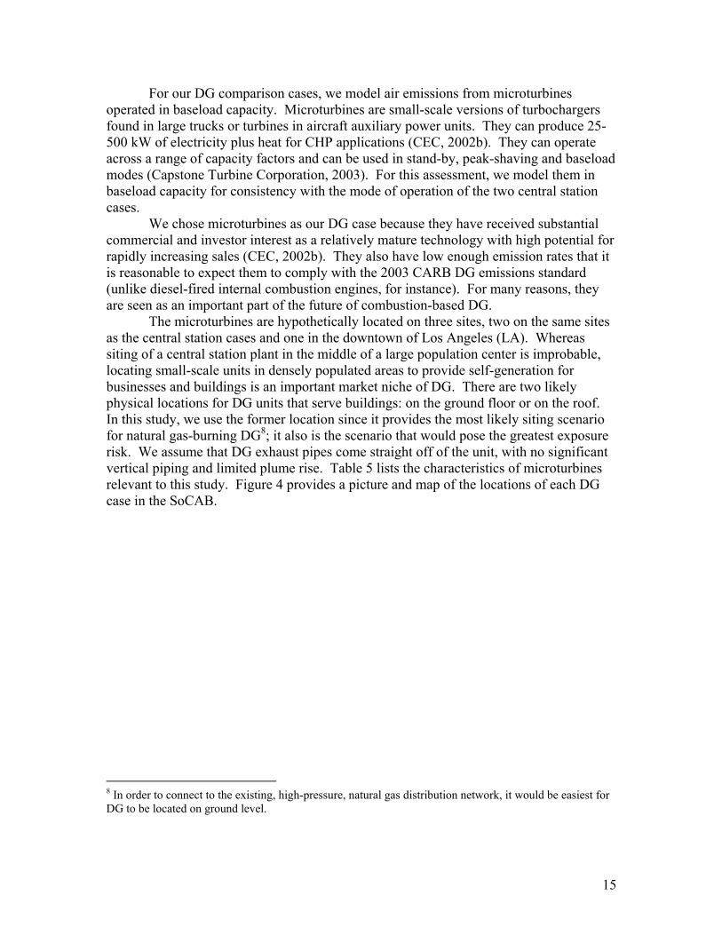
For our DG comparison cases, we model air emissions from microturbines operated in baseload capacity. Microturbines are small-scale versions of turbochargers found in large trucks or turbines in aircraft auxiliary power units. They can produce 25-500 kW of electricity plus heat for CHP applications (CEC, 2002b). They can operate across a range of capacity factors and can be used in stand-by, peak-shaving and baseload modes (Capstone Turbine Corporation, 2003). For this assessment, we model them in baseload capacity for consistency with the mode of operation of the two central station cases.

We chose microturbines as our DG case because they have received substantial commercial and investor interest as a relatively mature technology with high potential for rapidly increasing sales (CEC, 2002b). They also have low enough emission rates that it is reasonable to expect them to comply with the 2003 CARB DG emissions standard (unlike diesel-fired internal combustion engines, for instance). For many reasons, they are seen as an important part of the future of combustion-based DG.

The microturbines are hypothetically located on three sites, two on the same sites as the central station cases and one in the downtown of Los Angeles (LA). Whereas siting of a central station plant in the middle of a large population center is improbable, locating small-scale units in densely populated areas to provide self-generation for businesses and buildings is an important market niche of DG. There are two likely physical locations for DG units that serve buildings: on the ground floor or on the roof. In this study, we use the former location since it provides the most likely siting scenario for natural gas-burning DG8; it also is the scenario that would pose the greatest exposure risk. We assume that DG exhaust pipes come straight off of the unit, with no significant vertical piping and limited plume rise. Table 5 lists the characteristics of microturbines relevant to this study. Figure 4 provides a picture and map of the locations of each DG case in the SoCAB.

8 In order to connect to the existing, high-pressure, natural gas distribution network, it would be easiest for DG to be located on ground level.

15

Coun

tyAi

r Bas

inLo

catio

n Ty

pe

San

Luis

Obisp

oSo

uth

Cent

ral

Coas

tRu

ral

Coas

tal

Los A

ngele

sSo

uth

Coas

tSu

burb

an

Coas

tal

Los A

ngele

sSo

uth

Coas

tUr

ban

Down

town

a Effe

ctive

stac

k he

ight

is d

iscus

sed

in se

ction

II.C

.4.a.

Micr

otur

bine

Tech

nolo

gyFu

elCa

pacit

y (k

W)

30Na

tura

l Gas

52

25%

Case

Loc

atio

nEf

fect

ive S

tack

H

eight

a

(m)

Stac

k H

eight

(m

)Ef

ficien

cy

Tab

le 5

. M

odel

ing

char

acte

ristic

s of t

he th

ree

mic

rotu

rbin

e ca

ses r

elev

ant t

o ai

r qua

lity.

16

Figure 4. Map of locations of two of the three microturbine cases. A picture of a microturbine is provided to the left of the map (Capstone, 2002). A microturbine was also modeled at the site of the Morro Bay central station (see Figure 3). The tacks indicate the modeled locations.

17

II.B Pollutant Selection The pollutants modeled include one from each of two classes: conserved and

decaying. A hazard ranking formed the basis for selection of these pollutants (see section II.D.1 for the calculation method and section III.A for the detailed results). Primary emissions of particulate matter less than 2.5 micrometers in diameter (PM2.5) can be treated as a conserved species in outdoor air on the timescales of transport within 100 km and have one of the highest health risks attributable to electricity generation (Krewitt et al., 1998). 9 In this assessment, we assume that all primary emissions of particulate matter from natural gas combustion are in the form of PM2.5 (EPA, 2000). 10

Formaldehyde (HCHO) had the highest hazard ranking among the hazardous air pollutants we evaluated and so was selected to represent the case of a decaying pollutant. This assessment only considers formaldehyde exposures directly attributable to emissions from combustion of natural-gas used in generating electricity. Emissions of other volatile organic compounds (VOC) from natural-gas combustion are too low for secondary formation of formaldehyde due solely to this source to be important; thus, we only consider primary emissions in this assessment. 11

II.C Modeling Tools and Input Data

Sections II.C.1-4 report the various calculation methods, data sources and assumptions used in this study. II.C.1 Gaussian Plume Model II.C.1.a Gaussian Plume Model for Conserved Pollutants

We modeled downwind pollutant concentrations from the electricity generation sources using a standard Gaussian plume model (Turner, 1994). We limited our assessment of downwind concentration to within 100 km for three reasons. First, the dispersion parameters are generally not thought to be valid beyond this distance. Second, a similar assessment by Marshall (2002) found that the contribution to population intake beyond this distance is minor because of the low concentrations achieved after so much dilution. 12 This result is especially true for decaying species. Third, proper treatment of long-range transport would require the application of trajectory-tracking models with appropriate meteorological data, an approach that was beyond the resources available for 9 The atmospheric lifetime of PM2.5 was estimated by Seinfeld and Pandis (1998) as “many days”, which is greater than the transport time, assuming constant prevailing winds, from any of the cases we evaluate. Using deposition velocity data from Seinfeld and Pandis (1998) for PM of diameter 0.2-2 µm, we estimate losses over 100 km to be 1-8%. These small loss rates justify treating PM2.5 as a conserved pollutant. 10 There will be a difference in the average age of particles by the time they are inhaled by humans, with DG emissions, on average, being younger. This could have some impact on health consequences, but it is unclear at this time exactly how and how much. Thus, we leave this issue to further study. 11 There are many other sources of formaldehyde exposure in addition to primary emissions from natural gas combustion, including secondary formation from gaseous precursors (it has been estimated that greater than 75% of summer, daytime, urban formaldehyde is due to secondary formation (e.g., Friedfeld et al., 2002)), and primary emissions from motor vehicles, building materials, consumer products and industrial processes. 12 We note, however, that the work of Marshall (2002) focused on ground-based releases in the South Coast Air Basin. Significant contributions to intake fraction could occur for remote releases that impact heavily populated regions far downwind.

18

this study. For the purposes of examining the tradeoffs between the two paradigms of electricity generation in terms of human exposure, the 100 km domain seems acceptable.

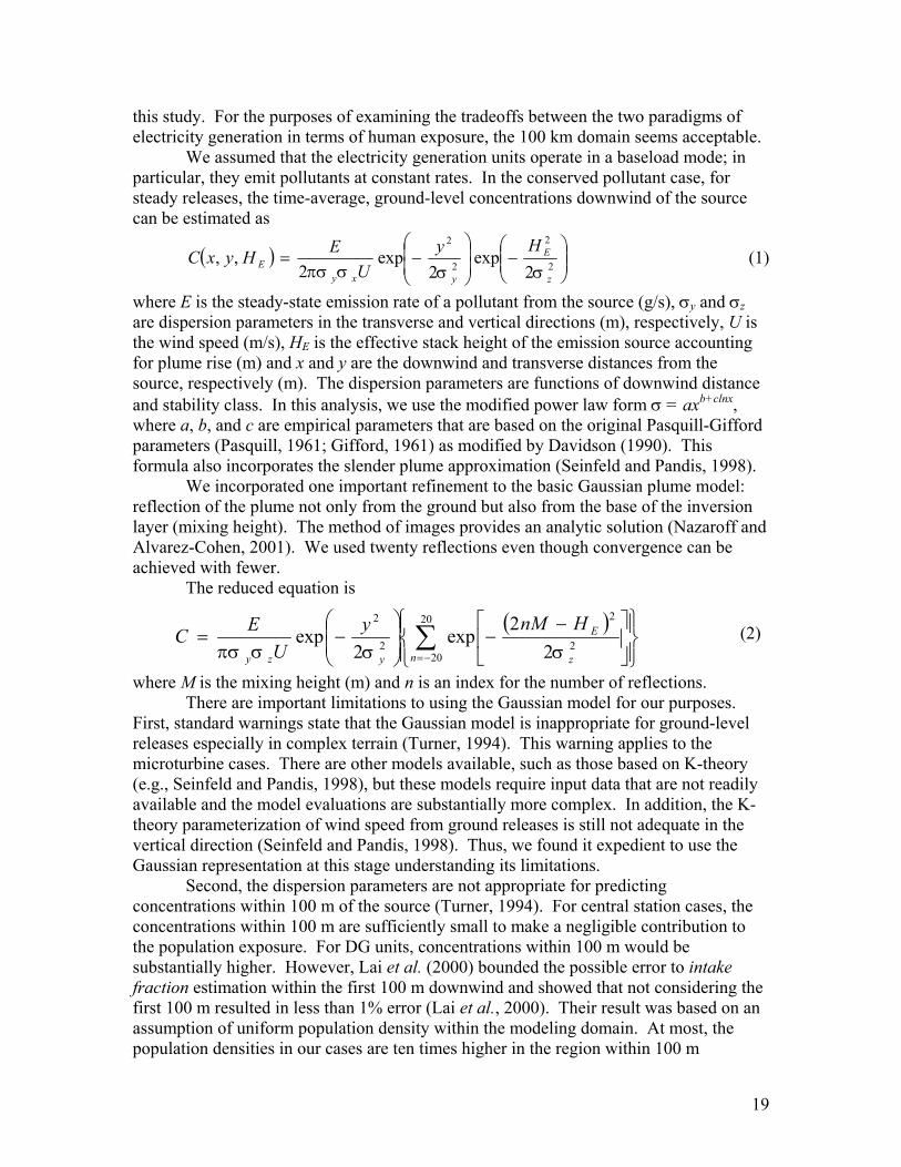
We assumed that the electricity generation units operate in a baseload mode; in particular, they emit pollutants at constant rates. In the conserved pollutant case, for steady releases, the time-average, ground-level concentrations downwind of the source can be estimated as

( )

−

−= 2

2

2

2

2exp

2exp

2,,

z

E

yxyE

HyU

EHyxCσσσπσ

(1)

where E is the steady-state emission rate of a pollutant from the source (g/s), σy and σz are dispersion parameters in the transverse and vertical directions (m), respectively, U is the wind speed (m/s), HE is the effective stack height of the emission source accounting for plume rise (m) and x and y are the downwind and transverse distances from the source, respectively (m). The dispersion parameters are functions of downwind distance and stability class. In this analysis, we use the modified power law form σ = axb+clnx, where a, b, and c are empirical parameters that are based on the original Pasquill-Gifford parameters (Pasquill, 1961; Gifford, 1961) as modified by Davidson (1990). This formula also incorporates the slender plume approximation (Seinfeld and Pandis, 1998).

We incorporated one important refinement to the basic Gaussian plume model: reflection of the plume not only from the ground but also from the base of the inversion layer (mixing height). The method of images provides an analytic solution (Nazaroff and Alvarez-Cohen, 2001). We used twenty reflections even though convergence can be achieved with fewer.

The reduced equation is

( )

−−

−= ∑

−=

20

202

2

2

2

22

exp2

expn z

E

yzy

HnMyU

ECσσσπσ

(2)

where M is the mixing height (m) and n is an index for the number of reflections. There are important limitations to using the Gaussian model for our purposes.

First, standard warnings state that the Gaussian model is inappropriate for ground-level releases especially in complex terrain (Turner, 1994). This warning applies to the microturbine cases. There are other models available, such as those based on K-theory (e.g., Seinfeld and Pandis, 1998), but these models require input data that are not readily available and the model evaluations are substantially more complex. In addition, the K-theory parameterization of wind speed from ground releases is still not adequate in the vertical direction (Seinfeld and Pandis, 1998). Thus, we found it expedient to use the Gaussian representation at this stage understanding its limitations.

Second, the dispersion parameters are not appropriate for predicting concentrations within 100 m of the source (Turner, 1994). For central station cases, the concentrations within 100 m are sufficiently small to make a negligible contribution to the population exposure. For DG units, concentrations within 100 m would be substantially higher. However, Lai et al. (2000) bounded the possible error to intake fraction estimation within the first 100 m downwind and showed that not considering the first 100 m resulted in less than 1% error (Lai et al., 2000). Their result was based on an assumption of uniform population density within the modeling domain. At most, the population densities in our cases are ten times higher in the region within 100 m

19

compared to the rest of the modeling domain, so we would expect 10% or less error if we excluded this region entirely. In fact, we estimate concentration within 100 m by extrapolating from a point beyond 100 m to the origin. Thus, we expect our error to be less than 10% owing to this factor.

Finally, the Pasquill stability class representation is discretized while the atmosphere is continuous in its conditions (see section II.C.2.c for further description of Pasquill classification system). As there are no other descriptions of atmospheric conditions as widely used and trusted as the Pasquill system, we deem its use here to be appropriate.

There are two other important assumptions. First, to use the Gaussian model, one must assume that meteorological conditions remain constant within the transport time of the plume (Turner, 1994). For this assessment, we draw the boundary of the exposed population at 100 km downwind in the prevailing wind direction. At the wind speeds in the prevailing direction, the travel time is approximately 13 hours and 7.5 hours in the cases of Morro Bay and the SoCAB locations, respectively. Clearly, meteorological conditions do not remain constant over intervals of the order of 10 h. However, what we seek in this study is closely related to the long-term temporal- and spatial-averaged ground-level concentration over the entire impact area of the plume. As the system is linear for the pollutants considered here, the assumption of steady state as a means to estimate an average is reasonable. Nevertheless, this issue should be addressed in future refinements of this line of research.

The second set of assumptions relate to the treatment of pollutant loss at the system boundaries, i.e., the ground and the bottom of the inversion layer. We assume that there is no loss of pollutant to the ground surface or through the inversion layer, i.e., that there is perfect reflection from those boundaries. While the assumption of perfect reflection at the ground surface may not be strictly true for PM2.5, we estimate that this assumption introduces an error of less than 10% over the travel distance of the plume. Thus, PM2.5 can be approximated as a conserved pollutant over the distances within the scope of this study.

As for pollutant loss at the upper boundary, for all cases where the effective stack height of a plant is lower than the mixing height, we assume the bottom of the inversion layer is perfectly reflecting. However, there are many hours of the year when the mixing height is lower than the effective stack height of the central station plants (the proportion is higher for Morro Bay since it has taller stacks). When considering population intake during those hours, we made the simplifying assumption that this condition was completely protective of public health, i.e., that the vertical plume from the stack has enough momentum to fully pass through the inversion base and be separated from the people below. Operationally, this means that we multiply our intake fraction values by a first-order correction term equal to the proportion of annual hours that the effective stack height is lower than the mixing height. II.C.1.b Gaussian Plume Model for Decaying Pollutants

The Gaussian plume model can easily incorporate first-order decay of primary pollutants by adding an exponential decay term to the expression. Thus, eq 2 becomes

( )UkxCC cd /exp −= (3)

20

where Cd is the concentration of the decaying species (g/m3), Cc is the concentration of a conserved species emitted at the same rate and under the same conditions as the decaying species (g/m3), k is the decay constant (s-1), U is the wind speed (m/s) and x is the downwind distance (m). If there are multiple loss mechanisms (such as for formaldehyde), the decay constant represents the sum of the rates of all applicable loss mechanisms. Similar to our assumption for the conserved pollutant PM2.5, we also assume no loss of formaldehyde to the ground surface. While its deposition velocity is higher than for PM2.5, leading to losses of approximately 30% over the travel distance of the plume (using data from Christensen et al., 2000), we leave the incorporation of this additional loss factor to future refinements of this line of research. II.C.2 Meteorological Parameters

Several meteorological parameters are used in the Gaussian plume model: mixing height, wind speed and direction, and stability class. Table 6 at the end of this section summarizes all of the relevant meteorological data for each case. II.C.2.a Mixing Height

For mixing height, we used the EPA Support Center for Regulatory Air Models data (EPA, 2002b). In this data set, there is only one station in California that records mixing height — Oakland — so its values were used for all cases; we selected the 1991 data because it was the most recent year available. While sources that provide mixing height data for other cities in California exist, they must often be purchased or used in conjunction with a preprocessor for one of the common air dispersion model packages. Thus, for this exploratory research, it was not practical to use these data.

We chose to use the harmonic mean of the data because the mixing height appears in the denominator of the equation for concentration in a well-mixed air basin (C = E (MWU)-1, where W is the width of the box). For conditions where the mixing height is low and the atmosphere is unstable, the Gaussian model matches the case of a well-mixed air basin. The harmonic mean of a set of data is different than its arithmetic mean and is the correct choice when the variable to be averaged appears in the denominator of a desired result.

The value of mixing height harmonic means was different between the microturbine and two central station cases. Plume reflection from the bottom of the inversion layer only occurs when the mixing height is higher than the effective stack height. Therefore, we only used the harmonic mean of those hours for which reflection occurs in the Gaussian model. In the special case of the very low effective stack height from microturbines, all hours have mixing heights above the effective stack height, so we use the harmonic mean of the complete data set. II.C.2.b Wind Speed and Direction

Wind speed and direction, as well as all of the parameters necessary to determine stability class, were taken from the National Renewable Energy Laboratory’s (NREL) Typical Meteorological Year 2 (TMY2) dataset (NREL, 1995). The TMY2 dataset consists of hourly solar radiation and meteorological elements for the period of one year. It is derived from the 1961-1990 National Solar Radiation Data Base and “represents conditions judged to be typical over a long period of time, such as 30 years” (NREL,

21

1995). It is intended for the comparison of computer simulations of energy systems; thus, it is appropriate for use in this assessment.

The histogram of wind direction in Los Angeles (the closest meteorological station to El Segundo and downtown LA) (Figure 5) shows a marked peak in the prevailing wind direction. This peak is centered around 250° (the onshore, daytime winds), with a second mode centered around 90° (the offshore, nighttime winds). A combined 78% of the TMY2 hours occur in one or the other mode. As a simplifying assumption, we treated the winds for LA as bimodal and allocated the remaining hours evenly between the two modes. The effect of a more robust treatment of wind direction is discussed in the Appendix to this report. Also, note that in the case of coastal plants (central and DG), when the winds are offshore, there is no population exposure. This is not true in the case of DG located in downtown LA, where there are ten kilometers of land (and people) before the offshore winds are blown to sea.

The histogram of wind direction for Santa Maria (closest meteorological station to Morro Bay) (Figure 6) displays a similar, though less pronounced, bimodal pattern, with 72% of the TMY2 hours fitting either mode. We treated the allocation of hours not occurring in either mode in the same manner as for Los Angeles.

22

0

200

400

600

800

1000

1200

1400

0 100 200 300

Wind Direction (degrees)

Nu

mb

er o

f O

ccu

ren

ces

26% of hours

Second Mode

PrevailingWind

Direction

51% of hours

Figure 5. Wind direction histogram for Los Angeles, CA, based on typical meteorological year data (TMY2) (NREL, 1995).

0

200

400

600

800

1000

1200

1400

1600

0 100 200 300

Wind Direction (degrees)

Nu

mb

er o

f O

ccu

ren

ces

Second Mode

16% of hours

Prevailing W ind Direction

51% of hours

Figure 6. Wind direction histogram for Santa Maria, CA, based on typical meteorological year data (TMY2) (NREL, 1995).

23

Because wind speed appears in the denominator of the Gaussian equation, we use the harmonic mean for all hours in each mode. However, there is still an issue of how to treat those hours that have zero measured wind speed (i.e., calm conditions); 4% and 7% of hours are calms for LA and for Santa Maria, respectively. Near-source concentrations increase monotonically with decreasing wind speed, such that periods of calm conditions could present a significant health risk for local exposure to air emissions, especially from ground-source releases but also for releases from tall stacks. By neglecting calms from the calculation of harmonic mean of wind speed, we expect to underpredict the true population exposure. However, because the proportion of hours with calm conditions is small for both locations, we do not expect the bias to be large. II.C.2.c Atmospheric Stability Class

We determined atmospheric stability for each hour in a year by applying the Pasquill classification system (Pasquill, 1961) to the TMY2 data. Atmospheric stability describes the relationship between mechanical turbulent mixing and the effect of buoyancy on an air parcel (Turner, 1994). “Unstable” conditions (Pasquill stability classes A through C) enhance vertical mixing while “stable” conditions (E and F) hinder it; D is the neutral condition. We use the prevalence of each stability class as the weights for averaging the results of the stability class-specific population intake evaluation to estimate an annual-average value.

There was not a perfect match between all requirements of Pasquill’s classification system and the TMY2 data. Consequently, we made the following translations. Where Turner reports that others have designated nighttime hours with winds less than 2 m/s as “G”, we classify these hours as “F” since there are no dispersion parameters in Davidson (1990) or common texts for “G.” Pasquill defines night as “the period 1 hour before sunset to 1 hour after sunrise” (Pasquill, 1961). The translation we use for the TMY2 data is one hour before “extraterrestrial horizontal radiation” is zero in evening and one hour after it is zero in the morning. To implement Pasquill’s requirement that "category D should be used, regardless of wind speed, for overcast conditions during day or night" (Pasquill, 1961), we defined overcast as when low clouds completely cover the sky (i.e., when "opaque sky cover" = 10 for the TMY2 data). Finally, for all cases where stability class is given as a range, we use the end of the range tending toward neutral conditions (e.g, for “A-B” we use “B”).

24

Dir

ectio

n%

of

hour

sSp

eed

(m/s

)D

irec

tion

% o

f ho

urs

Spee

d(m

/s)

AB

CD

EF

Cen

tral

St

atio

n74

4

DG

343

Cen

tral

St

atio

n62

6

DG

343

Dow

ntow

n LA

DG

343

Mor

ro B

ay

3.7

0.1%

2.3

38%

90o

62%

250o

Sant

a M

aria

Los A

ngel

es

Mix

ing

Hei

ght

(m)

Loca

tion

Met

eoro

logi

cal

Stat

ion

Prev

ailin

g W

ind

Seco

nd M

odal

Win

dPr

eval

ence

of S

tabi

lity

Cla

ss (%

) 22%

13%

43%

16%

300o

29%

9.8%

38%

14%

9.0%

El S

egun

do

Cas

e

6.8%

0.1%

1.9

30%

120o

2.1

70%

Tab

le 6

. Su

mm

ary

of m

eteo

rolo

gica

l dat

a fo

r eac

h ca

se.

25

II.C.3 Population Parameters To assess population exposures to air pollutants, there are two important factors

related to the exposed population: the number and the breathing rate of exposed people. Population density is heterogeneous, varying in both space and time. In the spatial dimension, we adopted two approaches. For the treatment presented in the body of this report, we considered population density as constant within counties, with the exception of Los Angeles city. A more detailed assessment that considers population resolved at the level of census tracts is discussed in the Appendix; a summary of the results from the Appendix is presented in section III.B.6. We used 2000 California Department of Finance, Demographic Research Unit population and county area data (as reported in CARB, 2001b) to determine county-level population density. For population density of Los Angeles city, we used the results of the 2000 U.S. Census and the area of the city (as reported in City of Los Angeles, 2001). We did not consider temporal variability in population density for this assessment. Figure 7 displays the population density figures used in this assessment as a function of downwind distance. The distance-weighted average densities are 1359 people/km2 for El Segundo and downtown LA, and 36 people/km2 for Morro Bay.

Breathing rates are also heterogeneous, varying by age, gender, level of activity, and health status. We assume a constant breathing rate equal to the estimated lifetime population-average value of 12 m3/d (Layton, 1993).

26

C)

0

10

20

30

40

50

60

0 20 40 60 80 100

Distance Downwind (km)

Po

pu

lati

on

Den

sity

(#/

km 2 )

3500

/km

2 )

0500

10001500200025003000

0 20 40 60 80 100op

ula

tio

n D

ensi

ty (

#

D istance D ow nw ind (km )

P

0

500

1000

1500

2000

2500

3000

3500

-10 10 30 50 70 90Distance Downwind (km )

Po

pu

lati

on

Den

sity

(#/

km2 )

Offshore Onshore

A)

B)

Figure 7A, B and C. Population density (people/km2) as a function of downwind distance for each of the three locations of electricity generation units: A) Morro Bay; B) El Segundo; and C) Downtown LA. Population densities are treated as constant within counties, with the exception of LA city (3047 people/km2). The microturbine located in downtown LA is ten kilometers inland from the ocean; “offshore” shows the population density in the offshore wind direction, while “onshore” shows the population density in the onshore wind direction. Morro Bay and El Segundo are located directly on the coast; thus, offshore winds expose no one.

27

II.C.4 Power Plant and Pollutant Data II.C.4.a Power Plant Data

Two factors related to the electricity generation units are key for exposure assessment: release height and pollutant emission rates. When a pollutant is released from a large combustion source, it is usually emitted from a stack with some exit velocity and elevated temperature. Both of these factors cause the plume to rise above the physical height of the stack before its net effective velocity aligns to that of the prevailing wind. The sum of the physical stack height plus the plume rise, i.e., the “effective stack height,” is the release height used in Gaussian plume models. There are multiple methods to calculate plume rise and determine the effective stack height (see Turner, 1994). For the central station facilities at Morro Bay and El Segundo, we used effective stack heights reported by the USEPA (EPA, 1996). For emissions from microturbines, we used an effective stack height of 5 m, nominally assuming that the emissions were near ground level and that the plume rise would be minimal due to the low volumetric flow and exit velocity. 13

There is one additional issue with regard to the central station stacks. El Segundo has two stacks of different physical and effective stack heights. For the Gaussian and population exposure calculations, we weighted the contribution of each stack by the corresponding flow of emissions, as reported by the EPA (EPA, 1996). Morro Bay has three stacks, but they are all the same height. 14 In this case, we treated all emissions as leaving from one stack. 15 The stack height data for each central station plant and microturbine are summarized in Tables 4 and 5, respectively.

Emission factors for each pollutant are necessary to conduct both the pollutant hazard ranking and to calculate the intake factor (see sections II.D.1 and II.D.3). For both assessments, examples of existing and new central station and DG technologies could be evaluated. We use existing central station and microturbine emission factors for the hazard ranking. This is consistent with the goal of a hazard ranking which is to assess potential hazard based on an upper-bound scenario (e.g., the higher emissions of microturbines installed before more strict regulations were enacted). Likewise, in order to establish baseline intake factors for the current mix of central stations and microturbines we use emission factors based on those existing technologies.

Another goal of our research is to estimate emission factors for new DG technologies necessary to equalize exposure burden to central station levels. Since new DG technologies could displace either existing or new central station production, we estimate intake factors for both; this requires estimating emission factors from new combined cycle turbines. Table 7 summarizes the emission factors used in these two assessments; the remainder of this section discusses the data and methods used to estimate emission factors. 13 It is possible for DG technologies to be located on the roofs of buildings. Even though the effective stack height above the building would still only be on the order of five meters, the height of the building would add considerably to the release height as used in Gaussian plume modeling. 14 Only two of the stacks have reported emissions (EPA, 1996) and those are nearly equal, further justifying modeling them as one stack. 15 By the time the plume has reached the ground, the plume width from each stack is an order of magnitude or more greater than the distance between the stacks. This justifies treating the emissions as if they were emitted from just one stack.

28

In the case of electricity generation, emission factors typically express the mass of pollutant emitted either per unit of heat input or per unit of electricity output. If emissions are reported per unit heat input, knowing the thermal energy-to-electricity conversion efficiency allows one to calculate the emission factor per unit of electricity generated. For the central station plants, we calculated the efficiency from heat input and electric output data provided by EPA’s Emission and Generation Resource Integrated Database (EPA, 1998). For consistency with the effective stack height data, we chose to use 1996 values.

Central station emission factors also need to be adjusted to account for the loss of electricity between where it is generated and where it is used (i.e., line loss). Electricity is converted to heat due to resistance (R) in the transmitting media and the amount of current (I) (Ph=I2R; where Ph is power which in this case is the rate of production of heat energy or electric power loss). This loss is a function of both distance (directly proportional to R) and voltage (V) (inversely proportional). 16 DG is superior to central stations on both counts. By definition, central station plants are more distant from where the electricity will be used than DG. In addition, by connecting to the customer side of the meter — the formal definition of DG (Ackerman et al., 2001) — DG units avoid the distribution part of the network, which has the lowest voltage. This latter factor is the more important one as a greater proportion of line losses occur in the distribution network than in the high-voltage, long-distance transmission lines (Ackermann et al., 2001). For the purposes of this assessment, we applied average line losses of 10% to electricity generated by central station plants and 0% for the microturbines in order to account for this benefit of DG (Energy Information Administration, 1999).

Emission rates (tons/year) are recorded for California central station plants in the state’s emission inventory (CARB, 2000b). We used 1996 data to be consistent with the reporting year for the effective stack height and efficiency. 17 Knowing the heat input, efficiency and line loss, we calculated emission factors in milligrams of a pollutant emitted per kilowatt-hour of electricity delivered (mg/kWhdel).

New central station plants in California are required to meet the CARB BACT standard for five pollutants: NOx, CO, VOC, PM10 and SO2 (CARB, 1999). In the case of PM10, the BACT recommendation is written as a limit on the amount of sulfur in natural gas. This formulation presents difficulties in translation to units of mass emission per kilowatt-hour. Instead, we used the requirements placed on a particular power plant that recently underwent BACT review (Carson Energy Group, Sacramento, CA) to estimate their PM10 emissions (CARB, 1999). We then assume that other new central station plants will be required to achieve similar emission reductions.

Since there is no BACT for formaldehyde, an emission factor was obtained from AP-42 (EPA, 2000), adjusted for the higher efficiency of these units (51%) (RAP, 2001). In this case, we assumed that all new central stations would be able to achieve an emission factor equivalent to facilities with catalytic reduction control technology installed.

16 With constant electric power demand, lower voltage requires increased current (Pe = IV; where Pe in this case is electric power). 17 Using more recent data (1999) does not change the results significantly. Thus, for consistency with the stack height data, we only display and discuss the results using the 1996 data.

29

For the DG cases, because the industry is so young, almost all technology-specific performance data are either unavailable or unconfirmed by independent testing. Fortunately, in the case of microturbines, the base technology is relatively mature and emission factors have been determined for a range of natural gas units. The most widely used emission factors handbook is the EPA’s Compilation of Air Pollutant Emission Factors, otherwise known as AP-42 (EPA, 2000). For microturbines installed before 2003 (for which the CARB emission standards do not apply), we use AP-42 emission factors to represent uncontrolled emissions of all pollutants.

Chapter 3.1 of AP-42 contains emission factors for criteria and hazardous air pollutants for natural gas turbines. Scaling the AP-42 factors (reported in pounds per million British thermal units, lbs/MMBtu) by the efficiency of microturbines provides the emission factors in units of mg/kWhdel. We estimated microturbine efficiency by averaging three values reported by manufacturers (Marnay, 2003). Table 7 displays emissions factors across a range of pollutants of concern used in modeling each case considered in this analysis.

We have simplified the analysis by assuming that the technologies will operate at the emission factor reported in Table 7 for every hour of a year, i.e., in steady-state. It is fair to ask whether this assumption will under- or over-estimate true annual-average population intake. The answer depends on the ratio of the amount of ‘negative’ emissions from periods of non-operation to the amount emitted during periods of higher-than-steady-state emissions.

In reality, even baseload power plants with high capacity factors will have some non-operation hours. These can be thought of as ‘negative’ emissions compared to our steady-state assumption. However, every period of non-operation has associated start-up and shut-down emissions. Emission factors for start-up and shut-down conditions can be considerably higher than those under steady-state operations (CARB, 1999 and EPA, 2000). In addition, it is unlikely that even baseload central station plants will operate at full-load for all operable hours. Part-load conditions are also known to often have substantially higher emission factors (CARB, 1999 and EPA, 2000). Thus, to understand the true population inhalation exposure due to the emissions from the technologies considered in this report, we would need to know the number of hours in non-operation and start-up, shut-down and part-load conditions and the emission factors for each mode. This level of detail is generally not available for real plants (e.g., Morro Bay and El Segundo) and is not yet reported generically for microturbines.

30

NO

x C

OSO

2PM

10PM

2.5 g

Ben

zene

Form

alde

hyde

Mor

ro B

ayb

500

200

350

500.

020.

2E

l Seg

undo

c30

010

06

2020

0.01

1N

ew C

entr

al S

tatio

ns d

3050

102

20.

042

Exi

stin

g M

icro

turb

ines

e20

0050

00.

005

f40

400.

074

a EFs

for M

orro

Bay

and

El S

egun

do a

re b

ased

on

actu

al e

mis

sion

s in

199

6 (C

AR

B, 2

000b

) for

con

sist

ency

with

the

late

st a

vaila

ble

data

on

stac

k

para

met

ers

(EPA

, 199

6), e

xcep

t Mor

ro B

ay S

O2 (

EPA

, 199

8); n

ew c

entra

l sta

tion

plan

ts a

re a

ssum

ed to

be

com

bine

d cy

cle

natu

ral g

as tu

rbin

es m

eetin

g

BA

CT

em

issi

on re

quire

men

ts, e

xcep

t tox

ic e

mis

sion

s w

hich

are

bas

ed o

n A

P-42

ass

umin

g EF

s no

hig

her t

han

achi

eved

by

cata

lytic

redu

ctio

n co

ntro

l

tech

nolo

gy (E

PA, 2

000)

; EFs

for e

xist

ing

mic

rotu

rbin

es (i

.e.,

inst

alle

d be

fore

200

3) a

re fo

r unc

ontro

lled

emis

sion

s ba

sed

on A

P-42

dat

a (E

PA, 2

000)

.b I

nput

dat

a: e

ffic

ienc

y =

33%

, hea

t inp

ut =

14,

248,

414

MM

Btu

(150

00 T

J) (E

PA, 1

998)

; lin

e lo

ss =

10%

.c I

nput

dat

a: e

ffic

ienc

y =

31%

, hea

t inp

ut =

12,

756,

384

MM

Btu

(135

00 T

J) (E

PA, 1

998)

; lin

e lo

ss =

10%

.d

Ass

umpt

ions

: 51%

eff

icie

ncy

(RA

P, 2

001)

; lin

e lo

ss =

10%

; ins

talla

tion

of c

atal

ytic

redu

ctio

n te

chno

logy

(or e

quiv

alen

t) is

ass

umed

.e A

ssum

ptio

ns: 2

5% e

ffic

ienc

y (M

arna

y, 2

003)

; 0%

line

loss

. f E

mis

sion

fact

or g

iven

by

perc

ent s

ulfu

r con

tent

in n

atur

al g

as.

A

ssum

ptio

n: 9

x 1

0-7 w

eigh

t per

cent

of s

ulfu

r in

natu

ral g

as (U

nion

Gas

, 200

2) a

nd th

at a

ll SO

x are

SO

2.g

A

ssum

ing

that

all

PM e

mis

sion

s ar

e PM

2.5.

New

cen

tral s

tatio

ns e

stim

ate

base

d on

BA

CT

for C

arso

n En

ergy

Gro

up (C

AR

B, 1

999)

.

Ele

ctri

city

Gen

erat

ion

Uni

tC

rite

ria

Pollu

tant

sT

oxic

s

Em

issi

on F

acto

rsa

(mg/

kWh d

el)

Tab

le 7

. Em

issi

on fa

ctor

s use

d in

mod

elin

g th

e th

ree

cent

ral s

tatio

n ca

ses (

Mor

ro B

ay, E

l Seg

undo

and

new

cen

tral s

tatio

ns)

and

exis

ting

mic

rotu

rbin

es.

31

II.C.4.b Pollutant Data Two pollutant classes are considered. Because conserved pollutants, by

definition, undergo no transformations, no pollutant-specific data are needed in the Gaussian model to predict downwind concentrations. Decaying pollutants can be accommodated in Gaussian models with an exponential decay term, e-kx/U. The decay constant, k, represents the sum of all relevant loss mechanisms. In the case of formaldehyde, there are two reactions that contribute to the decay of this species on timescales of interest: photolysis and reaction with the hydroxyl radical (OH) (Atkinson, 2000). 18

The photolysis rate depends on solar intensity, which, in turn, varies with the time of day and year and latitude. Using data from Demerjian et al. (1980) on rates by zenith angle and path, and from Finlayson-Pitts and Pitts (1986) correlating zenith angle and time of day for Los Angeles, we estimated the average photolysis rate for ‘typical’ conditions during the six hours symmetric around noon.

Formaldehyde reaction with the OH radical is a first-order process. With data from Finlayson-Pitts and Pitts (1986) on OH concentration across a range of background pollution levels and the International Union of Pure and Applied Chemistry (IUPAC) recommended reaction rate (IUPAC, 2001), we estimated the reaction rate for two general pollution conditions. We modeled Morro Bay using “rural” conditions and El Segundo using “moderate” conditions. 19 Each OH background pollution level is reported over a range of concentration; we used the high end of each range. Table 8 summarizes the reaction rates used for formaldehyde decay.

18 In this assessment, we did not consider reaction with the nitrate radical (NO3) or dry or wet deposition of HCHO. Reaction with NO3, though the only significant loss mechanism during night, is relatively insignificant compared to losses by OH and photolysis during the day (Atkinson, 2000). Our central estimate for the effect of dry deposition on HCHO concentration is 30% loss within 100 km (using data from Christensen et al., 2000); this is small in comparison to the central estimate of 30-50% per hour loss by reactions. In future assessments, the role of dry and wet deposition would be worth exploring in more detail. 19 Even though El Segundo is just upwind of Los Angeles, one of the most polluted cities in the United States, since the plume will also travel over rural areas within the 100 km modeling domain, moderate conditions seemed a more appropriate average condition.

32

Zeni

th A

ngle

cR

ate

(h-1

)H

igh

End

Low

End

Hig

h En

dLo

w E

nd

30o

0.27

0.35

0.28

0.60

0.31

65o

0.10

0.19

0.11

0.43

0.15

45o

0.21

0.30

0.22

0.54

0.25

a OH

+ H

CH

O re

actio

n ra

te:

9.2x

10-1

2 cm

3 /(mol

ec s)

(IU

PAC

, 200

1)b [O

H] (

rura

l) =

2.5x

106 m

olec

/cm

3 ; [O

H] (

mod

erat

e) =

9.8

x106 m

olec

/cm

3 (hig

h en

d of

eac

h co

ncen

tratio

n ra

nge)

the

ave

rage

con

ditio

ns fo

r the

6 h

our b

lock

sym

met

ric a

roun

d no

on.

c 45o is

the

zent

h an

gle

at 1

0am

/2pm

on

the

equi

noxe

s in

LA. T

his t

ypic

al v

alue

repr

esen

ts a

ppro

xim

atel

y

Atm

Con

ditio

n--L

ow

Pollu

tion

(rur

al) b

Atm

Con

ditio

n--M

oder

ate

Pollu

tion b

Tot

al d

aytim

e ra

te c

onst

ant (

h-1)

Phot

olys

is(H

CO

and

H2 p

aths

)

(Fin

lays

on-P

itts a

nd P

itts,

1986

). M

orro

Bay

is m

odel

led

with

"ru

ral"

and

El S

egun

do w

ith "

mod

erat

e" c

ondi

tions

.

Tab

le 8

. To

tal d

aytim

e ra

te c

onst

ant f

or H

CH

O d

ecay

con

side

ring

reac

tion

with

the

hydr

oxyl

radi

cal (

OH

)a and

pho

toly

sis (

rate

s us

ed in

mod

elin

g in

bol

d).

33

II.D Modeled Parameters II.D.1 Hazard Index

The results of a hazard ranking were used to determine the pollutants for which to model population exposures (see Table 9). The figure of merit is an emission factor divided by a concentration guideline appropriate to the health effects of interest. With example units, the equation can be expressed as

(4) [ ] [ ]kWhEmission Hazard =kWhm

mmg

mg 3

3Guidelineion Concentrat

FactorIndex ==

This figure is similar to that used by the California Office of Environmental

Health Hazard Assessment (OEHHA) in their prioritization of toxic air contaminants for evaluating risks to children’s health (OEHHA, 2001a). By replacing their ambient concentration term with an emission factor, the figure used here represents a source-oriented, technology-specific hazard potential. The units (e.g., m3/kWh) suggest an alternative interpretation. This hazard index represents the minimum volume of air needed to dilute the amount of pollutant emitted during the production of one kilowatt-hour of electric energy to a level not considered hazardous to human health.

The emission factors are plant-specific in the cases of Morro Bay and El Segundo and generic for microturbines. We use emission factors for existing microturbines (i.e., those installed before the CARB 2003 DG emission standard was enacted) in order to assess an upper-bound potential hazard microturbines could pose.

A series of four hazard rankings used different concentration guidelines. We assume that the primary NAAQS (EPA, 2001) with the shortest averaging time (usually 24 h) are appropriate to assess risk of acute health outcomes (Scorecard, 2002a). We used the primary NAAQS with the longest averaging time (usually 1 y) to assess chronic, non-cancer outcomes (Scorecard, 2002a). 20 We evaluated chronic, non-cancer outcomes with chronic inhalation reference concentrations (mainly, chronic Reference Exposure Levels, RELs21) (OEHHA, 2001b). Finally, we also included an assessment of the relative cancer risk. 22 We used inhalation cancer potency factors (mainly, inhalation unit risk factors) to assess cancer outcomes (OEHHA, 1999).

Often, there are multiple agencies have issued guidelines for the same pollutant and health outcome. The selection of which guideline to use (within each of the four hazard rankings outlined above) was based on a prioritization scheme developed by Scorecard (2002b). When multiple agencies have developed a concentration guideline for the same chemical, Scorecard selects values from the agency with the largest number

20 The exception to this method is for NO2, where we use the annual-average NAAQS standard for both an acute and chronic assessment. Even though different averaging times are not required in the standard, NO2 has both acute and chronic health effects. 21 “A chronic REL is an airborne level that would pose no significant health risk to individuals indefinitely exposed to that level” (OEHHA, 2002). RELs cover a wider range of pollutants than NAAQS. In addition, because they use different criteria in their evaluation, where there is overlap to the NAAQS, they may be set at different levels. 22 It should be noted that this assessment does not produce the same units of hazard index as the previous three since the standard units for measuring carcinogenicity are cancer risk per milligram per kilogram body weight per day.

34

of concentration guidelines available. This prioritization scheme was adopted to ensure as much consistency as possible in the compilation of concentration guidelines. In our assessments, we used the values as selected by Scorecard.

We used a “weight of evidence” method to determine which pollutants to model. If a particular pollutant had a higher hazard ranking in, for instance, two of three assessments compared to other pollutants of its class (i.e., conserved or decaying), then we selected that pollutant to model. II.D.2 Intake Fraction

A figure of merit for the assessment of the difference in population exposure due to choice of electricity generation paradigm — central station or DG — is the intake fraction (iF). An iF is the fraction of an emitted pollutant that is inhaled by all exposed people, defined by Lai et al. (2000) as (5)

( ) ( )

( )∫

∑ ∫==

dttE

dttQtCiF people

B

emitted masspersons)exposed all(by inhaled mass

where C(t) is the time-varying concentration within the breathing zone attributable to the emission source (g/m3), QB(t) is the time-varying breathing rate (m3/h) and E(t) is the emission rate of the pollutant from the source in question (g/h). For steady releases, the numerator and denominator can be expressed as constant rates: (6)

E

CQiF people

B∑==

rateemission massrate inhalation mass

The concept of a ratio of inhaled mass to emitted mass has been used for over a decade, often under different names (see Bennett et al., 2002 for a historical summary). The iF metric combines the results of a pollutant fate and transport analysis with an exposure assessment to express the emissions-to-intake relationship in a single, dimensionless and intuitive value. Results for ambient emissions are usually expressed per million, e.g., grams of PM2.5 inhaled per metric ton emitted. 23 Principally, the iF depends on three factors: 1) the proximity between the source and the receptors; 2) the persistence of the pollutant emitted; and 3) the population density in the receptor region. Thus, the iF is more site-specific than technology-specific. For instance, note the lack of dependence on emission rate in the formulation of the iF.

The iF concept can be extended to evaluate source-receptor relationships for an individual, a group of individuals, or the entire exposed population. In the body of this report, the entire downwind exposed population within 100 km will be considered. In the Appendix, the apportionment of iF among selected subpopulations is explored.

A few features of the iF are noteworthy, especially in contrast to alternative methods of estimating risk from electricity generation stations. A traditional approach to estimating the risk posed by HAP emissions from large, central station power plants involves estimating the lifetime intake of a hypothetical person who breathes the maximum ground-level concentration (in both time and space) of a pollutant (e.g., AB

35

23 Indoor releases usually lead to iFs in the hundredth to thousandth range, because of slower removal by airflow and smaller mixing volumes (Lai et al., 2000).

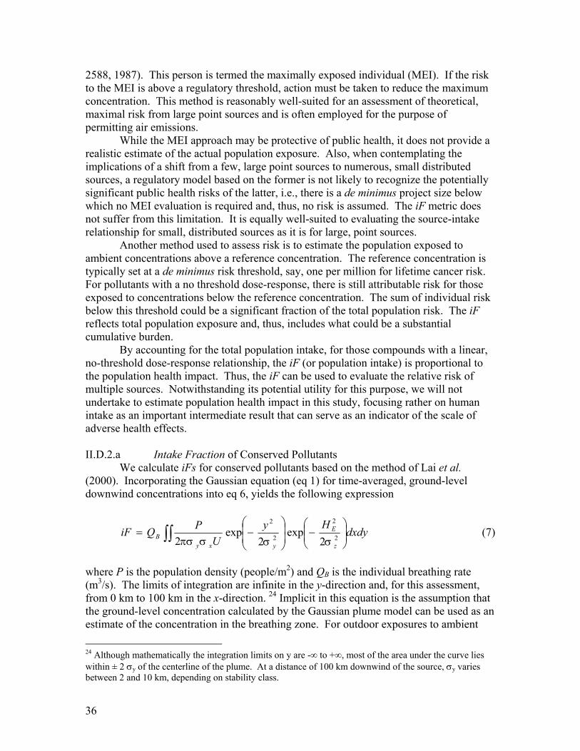
2588, 1987). This person is termed the maximally exposed individual (MEI). If the risk to the MEI is above a regulatory threshold, action must be taken to reduce the maximum concentration. This method is reasonably well-suited for an assessment of theoretical, maximal risk from large point sources and is often employed for the purpose of permitting air emissions.

While the MEI approach may be protective of public health, it does not provide a realistic estimate of the actual population exposure. Also, when contemplating the implications of a shift from a few, large point sources to numerous, small distributed sources, a regulatory model based on the former is not likely to recognize the potentially significant public health risks of the latter, i.e., there is a de minimus project size below which no MEI evaluation is required and, thus, no risk is assumed. The iF metric does not suffer from this limitation. It is equally well-suited to evaluating the source-intake relationship for small, distributed sources as it is for large, point sources.

Another method used to assess risk is to estimate the population exposed to ambient concentrations above a reference concentration. The reference concentration is typically set at a de minimus risk threshold, say, one per million for lifetime cancer risk. For pollutants with a no threshold dose-response, there is still attributable risk for those exposed to concentrations below the reference concentration. The sum of individual risk below this threshold could be a significant fraction of the total population risk. The iF reflects total population exposure and, thus, includes what could be a substantial cumulative burden.

By accounting for the total population intake, for those compounds with a linear, no-threshold dose-response relationship, the iF (or population intake) is proportional to the population health impact. Thus, the iF can be used to evaluate the relative risk of multiple sources. Notwithstanding its potential utility for this purpose, we will not undertake to estimate population health impact in this study, focusing rather on human intake as an important intermediate result that can serve as an indicator of the scale of adverse health effects. II.D.2.a Intake Fraction of Conserved Pollutants

We calculate iFs for conserved pollutants based on the method of Lai et al. (2000). Incorporating the Gaussian equation (eq 1) for time-averaged, ground-level downwind concentrations into eq 6, yields the following expression

dxdyHy

UPQiF

z

E

yxyB

−

−= ∫∫ 2

2

2

2

2exp

2exp

2 σσσπσ (7)

where P is the population density (people/m2) and QB is the individual breathing rate (m3/s). The limits of integration are infinite in the y-direction and, for this assessment, from 0 km to 100 km in the x-direction. 24 Implicit in this equation is the assumption that the ground-level concentration calculated by the Gaussian plume model can be used as an estimate of the concentration in the breathing zone. For outdoor exposures to ambient

24 Although mathematically the integration limits on y are -∞ to +∞, most of the area under the curve lies within ± 2 σy of the centerline of the plume. At a distance of 100 km downwind of the source, σy varies between 2 and 10 km, depending on stability class.

36

concentrations, this assumption is reasonable. However, for certain pollutants such as PM2.5, being indoors offers some protection against pollutants of outdoor origin (Riley et al., 2002). To the extent that buildings are protective, our approach will overestimate the true intake fraction. However, it will do so in a consistent manner among different technologies, so that the proportional change in intake fraction across scenarios should not be biased by this effect.

By assuming infinite plume spread and constant population density in the transverse direction, eq 7 can be integrated analytically in the y-direction and numerically in the x-direction.25 The reduced expression for the iF of a conserved pollutant, including ground and mixing height reflection (with n = 20 reflections included to ensure convergence), is

(8)

( )dx

HnMPU

QiF

X

n z

E

z

B ∫ ∑

−−=

−=

max

0

20

202

2

22

exp2

σσπ

The limit of integration is 0 to xmax = 100 km in the x-direction. It is worth reiterating that the iF results for conserved pollutants are not dependent

on the particular pollutant chosen. Because intake fractions are normalized by the pollutant-specific emission rate, the modeled iF only depends on dispersion, power plant and population parameters. Thus, the results for conserved pollutants apply to this entire class of pollutants. II.D.2.b Intake Fraction for a Decaying Pollutant Intake fractions for decaying pollutants can be calculated by inserting Guassian-predicted concentrations modified by an exponential loss term (see eq 3) into eq 6. II.D.3 Intake Factor

To make the results of the iF assessment technology-specific and to account for some of the benefits of DG, e.g. reduced line loss, the pollutant-specific iFs are multiplied by appropriate emission factors. This method yields a parameter we call the intake factor (iFac), which quantifies pollutant intake per unit of electricity delivered. It can be used like an emissions factor to assess the potential damage of an activity (e.g., mass emitted) with knowledge only of its intensity (e.g., electricity generated). In this case, the intake factor indicates the population intake (grams inhaled) of air pollutants emitted because of the delivery of a certain amount of electricity to where it is used.

In equation form,

)(kWhdelivered yelectricit )(mg intakepopulation

delivered

inhaled=×= iFEFiFac (9) where EF is the emission factor expressed in pollutant mass emitted per unit electricity delivered (mgemitted/kWhdel). This figure of merit will be used as the ultimate point of comparison between the cases in our research.

37

25 We used a trapezoidal numerical integration scheme with a step size of ∆x = 0.5 km.

III. Results and Discussion

In this section, we will first present the results of the hazard ranking of pollutants emitted from the two central station plants and from microturbines. These results informed the decision of which pollutants to consider when evaluating population exposures. Differences in population exposure to air emissions from the two paradigms of electricity generation — central station and DG — are examined through the use of intake fractions. We will present the iF results for the electricity generation cases described in section II.A across a range of typical meteorological conditions for each location and for both a conserved species (PM2.5) and a decaying pollutant (formaldehyde). These results are then weighted by the prevalence of the meteorological conditions to estimate an annual-average intake fraction. We use these results to explore the relative exposure intensities (mass inhaled per mass emitted) from the different paradigms of electricity generation. To better understand the results, we systematically varied key parameters to reveal which are most influential in determining population exposure; results of this assessment are presented in section III.B.2. Finally, we normalized our site-specific intake fraction results by appropriate emission factors to achieve technology-specific intake factors (iFac). These results are used to compare the power plants and technologies in terms of pollutant mass inhaled per unit of electricity delivered. III.A Hazard Ranking Results

Results of the hazard ranking are presented in Table 9. Only pollutants with emission factors for all technologies (Morro Bay, El Segundo and micorturbines) were assessed. Emissions of trace metals from Morro Bay are shown for reference only. While the risks from metals for cancer and chronic noncancer outcomes (using reference concentrations) are high by comparison with other pollutants, since they were not consistently reported for all technologies we were unable to use them in this hazard ranking. It should also be repeated that our ranking only assesses the hazards attributable to the primary emissions of a particular pollutant from the three plants/technologies listed above, all of which are due to the combustion of natural gas for electricity generation. Thus, this hazard ranking does not represent a total exposure assessment to each pollutant, e.g., it does not consider other primary emissions or secondary formation.

38

Tab

le 9

: H

azar

d ra

nkin

g fo

r Mor

ro B

ay a

nd E

l Seg

undo

cen

tral s

tatio

n pl

ants

and

for e

xist

ing

mic

rotu

rbin

es.

Mor

ro B

ayb

El S

egun

doc

Mic

rotu

rbin

esd

Mor

ro B

ayE

l Seg

undo

Mic

rotu

rbin

esM

orro

Bay

El S

egun

doM

icro

turb

ines

Mor

ro B

ayE

l Seg

undo

Mic

rotu

rbin

esM

orro

Bay

El S

egun

doM

icro

turb

ines

Cri

teri

a P

ollu

tan

ts

NO

xe50

030

02,

000

20,0

0020

,000

100,

000

5,00

03,

000

20,0

005,

000

3,00

020

,000

CO

200

100

400

1010

504

210

SO2

36

0.00

5 f

49

0.00

840

700.

062

40.

004

PM

1050

208

1,00

040

080

030

010

030

0

PM

2.5g

5020

83,

000

1,00

02,

000

800

300

600

PM

2.5

(pri

mar

y +

sec

onda

ry)

h14

050

209,

000

3,00

08,

000

2,00

080

02,

000

Tox

ics

Ben

zene

0.02

0.01

0.07

0.00

050.

0004

0.00

20.

30.

21

Form

alde

hyde

0.2

14

0.00

10.

006

0.02

6040

01,

000

Tra

ce M

etal

si

Chr

omiu

m (

VI)

0.00

090.

19,

000

Nic

kel

0.3

0.08

6,00

0

Pho

spho

rous

0.4

6,00

0

a The

EF

s fo

r m

icro

turb

ines

are

bas

ed o

n A

P-4

2 (E

PA

, 200

0) f

or u

ncon

trol

led

emis

sion

s fr

om u

nits

inst

alle

d be

fore

the

CA

RB

200

3 e A

ssum

ing

all N

Ox

is in

the

form

of

NO

2 w

hen

inha

led

by h

uman

s.

D

G e

mis

sion

s st

anda

rd; f

or M

orro

Bay

and

El S

egun

do, E

Fs

are

base

d on

act

ual e

mis

sion

s in

199

6 (C

AR

B, 2

000b

) fo

r co

nsis

tenc

yf E

mis

sion

fac

tor

give

n by

per

cent

sul

fur

cont

ent i

n na

tura

l gas

. A

ssum

ptio

n: 9

x 1

0-7 w

eigh

t per

cent

of

sulf

ur in

nat

ural

gas

(U

nion

Gas

, 200

2)

w

ith

the

late

st a

vail

able

dat

a on

sta

ck p

aram

eter

s (E

PA, 1

996)

, exc

ept M

orro

Bay

SO

2 (E

PA

, 199

8).

an

d th

at a

ll SO

x are

in th

e fo

rm o

f SO

2.b I

nput

dat

a: e

ffic

ienc

y =

33%

, hea

t inp

ut =

14,

248,

414

MM

Btu

(15

000

TJ)

(E

PA

, 199

8); l

ine

loss

= 1

0%.

g A

ssum

ing

that

all

PM

em

issi

ons

are

in th

e fo

rm o

f PM

2.5.

c I

nput

dat

a: e

ffic

ienc

y =

31%

, hea

t inp

ut =

12,

756,

384

MM

Btu

(13

500

TJ)

(E

PA

, 199

8); l

ine

loss

= 1

0%.

h L

evy,

et.

al. (

1999

) m

odel

led

that

eve

ry g

ram

of

prim

ary

PM is

ass

ocia

ted

with

1.8

g o

f se

cond

ary

PM.

d Ass

umpt

ions

: 25%

eff

icie

ncy

(Mar

nay,

200

3) a

nd 0

% li

ne lo

ss.

i E

mis

sion

s fo

r tr

ace

met

als

wer

e on

ly r

epor

ted

for

the

case

of

Mor

ro B

ay (

EPA

, 200

0 an

d C

AR

B, 2

000b

).H

azar

d R

anki

ng S

ourc

es:

j Inh

alat

ion

canc

er p

oten

cy f

acto

rs (

mai

nly

inha

lati

on u

nit r

isk)

: OE

HH

A, 1

999.

Not

e: t

he c

ance

r in

dex

has

diff

eren

t uni

ts th

an th

e no

n-ca

ncer

out

com

es.

k Chr

onic

inha

lati

on r

efer

ence

con

cent

rati

ons

(mai

nly

chro

nic

Ref

eren

ce E

xpos

ure

Lev

els)

: OE

HH

A, 2

001b

.

Prim

ary

NA

AQ

S (E

PA, 2

001)

wit

h th

e lo

nges

t ave

ragi

ng ti

me

(usu

ally

one

yea

r) a

sses

s ch

roni

c, n

on-c

ance

r ou

tcom

es (

Scor

ecar

d, 2

002a

).

Pri

mar

y N

AA

QS

(E

PA

, 200

1) w

ith

the

shor

test

ave

ragi

ng ti

me

(usu

ally

24

hour

s) a

sses

s ac

ute

heal

th o

utco

mes

(S

core

card

, 200

2a).

39

Ch

emic

al(E

F / i

nhal

atio

n ca

ncer

pot

ency

fac

torj )

(EF

/ chr

onic

inha

latio

n R

efC

k)

(EF

/ NA

AQ

S)

Em

issi

on F

acto

rsa

(mg/

kWh d

el)

(EF

/ NA

AQ

S)

Haz

ard

Ran

king

Can

cer

Chr

onic

, Non

canc

erC

hron

ic, N

onca

ncer

Acu

te

(m

3 /kW

h del)

It is clear from Table 9 that the risks from certain pollutants are much higher than from others. Because each of the four rankings assesses a different health outcome and usually uses a different risk value (which were derived for different purposes) sometimes with different units (i.e., the cancer results), one should only compare the quantitative results within a category. PM2.5 (whether considering primary emissions alone or primary emissions plus secondary formation) displays the highest risk for conserved pollutants in both assessments using the NAAQS. 26 Formaldehyde displays the highest risk for decaying pollutants in both the cancer and chronic noncancer assessments (based on the chronic inhalation reference concentration). Thus, PM2.5 and formaldehyde are the two pollutants we selected for pollutant-specific iF and iFac assessments. 27

Based on this hazard ranking, NOx appears to pose the highest risk of any pollutant. However, NO2 — the pollutant for which there are health standards — is a secondary pollutant and modeling its formation and decay chemistry is complex. At this stage, our model cannot accurately assess human exposure to secondary pollutants such as NOx because it does not incorporate such necessary features as spatially and time-varying background concentrations of other reactive pollutants. Thus, we must leave the assessment of population exposure to NOx from electricity generation for future refinements of this research. III.B Intake Fraction Results III.B.1 Conserved Pollutants Results

Conserved pollutant intake fraction results for each case are presented in Figure 8 for a range of stability classes. The results in this section are applicable to any conserved pollutant as no pollutant-specific adjustments have been made.

A difference in the pattern of iF across stability class is immediately noticeable when comparing the central station to DG results (Figures 8A-B vs. Figures 8C-E). With increasing atmospheric stability (from A to F), there is a protective effect (i.e., lower intake fraction) when pollutants are emitted from tall stacks. More stable conditions mean that longer distances are required for the plume to reach the population on the ground leading to insignificant exposure for a substantial portion of the downwind population. For ground-level releases (i.e., the DG cases), increasing atmospheric stability enhances population intake as the vertical spread of the plume is hindered.

26 Carbon monoxide (CO) and benzene were the only other conserved pollutants assessed. Benzene is not formally comparable to either CO or PM2.5 since they have not been assessed under the same regulations. However, it seems safe to conclude from these results that the risks from benzene of these natural gas combustion sources are less than from PM2.5. 27 Of course, a complete exposure assessment of natural gas-based electricity generation must consider emissions from all pollutants, including all of those in Table 9.

40

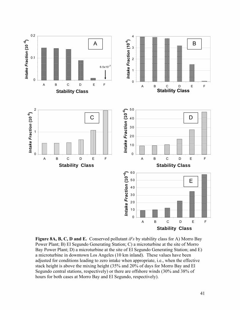
0

0 .1

0 .2

A B C D E F

Stability Class

Inta

ke F

ract

ion

(10

-6 )

6.5x10-7

���������������������������

�����������

���������������������������

����������������������

��������������������������������������

�����������

�������������������������

���������

�������������������

����� ������������������

0

1

2

3

4

A B C D E FStability Class

Inta

ke F

ract

ion

(10-6

)

A B

Figure 8A, B, C, D and E. Conserved pollutant iFs by stability class for A) Morro Bay Power Plant; B) El Segundo Generating Station; C) a microturbine at the site of Morro Bay Power Plant; D) a microturbine at the site of El Segundo Generating Station; and E) a microturbine in downtown Los Angeles (10 km inland). These values have been adjusted for conditions leading to zero intake when appropriate, i.e., when the effective stack height is above the mixing height (35% and 20% of days for Morro Bay and El Segundo central stations, respectively) or there are offshore winds (30% and 38% of hours for both cases at Morro Bay and El Segundo, respectively).

C

0

1

2

A B C D E F

Stability Class

Inta

ke F

ract

ion

(10

-6)

0

1 0

2 0

3 0

4 0

5 0

A B C D E F

Stability Class

Inta

ke F

ract

ion

(10

-6)

D

0

1 0

2 0

3 0

4 0

5 0

6 0

A B C D E F

Stability Class

Inta

ke F

ract

ion

(10

- 6)

E

41

Figure 9 compares the annual-average iF across all cases, weighted by the prevalence of stability class for each location. This figure reveals two important points. First, for the same location, lowering stack height from a central station level (hundreds of meters) to a typical DG level (5 m) increases the iF by approximately an order of magnitude. Recalling the three key influences on iF, lowering the stack height increases proximity by decreasing the (vertical) distance between the source and receptors. The result is higher ground-level concentrations per unit mass emitted and, consequently, higher intake. Second, changing from a rural to an urban location also increases the iF by an order of magnitude. In this instance, the proportionate influence of each of the many changing variables (downwind population density and meteorological conditions, in addition to stack height in the central station cases) is not obvious. An analysis of this question will be presented in section III.B.2.

Comparing the iF results in Figure 9 for DG at El Segundo vs. downtown Los Angeles raises an interesting question. With the same meteorological conditions, stack height and only slightly offset downwind population density, why is the iF for the DG unit in downtown LA (29 per million) higher than at El Segundo (23 per million)? The exact difference is mainly due to the specific circumstances of the comparison, but is based on general principles of the iF worth consideration here.

In the meteorological data for Los Angeles, the average wind speed in the offshore direction is slightly lower than for the onshore winds. For downtown LA, this leads to a higher iF within the distance to the ocean (10 km) compared to the iF over the same downwind distance when the prevailing onshore wind occurs. For ground-level releases and constant population density, greater incremental intake occurs closer to the source where the plume is more concentrated. Consequently, for the downtown LA case, the “gain” of ten kilometers of adjacent, exposed population in the offshore direction (compared to the El Segundo location) is greater in terms of population intake than the “loss” of ten kilometers of more distant exposed population in the prevailing wind direction. While the total population intake over the distance of the plume is greater in the prevailing wind direction, the particular combination of bimodally distributed winds in LA creates the outcome observed in Figure 9.

42

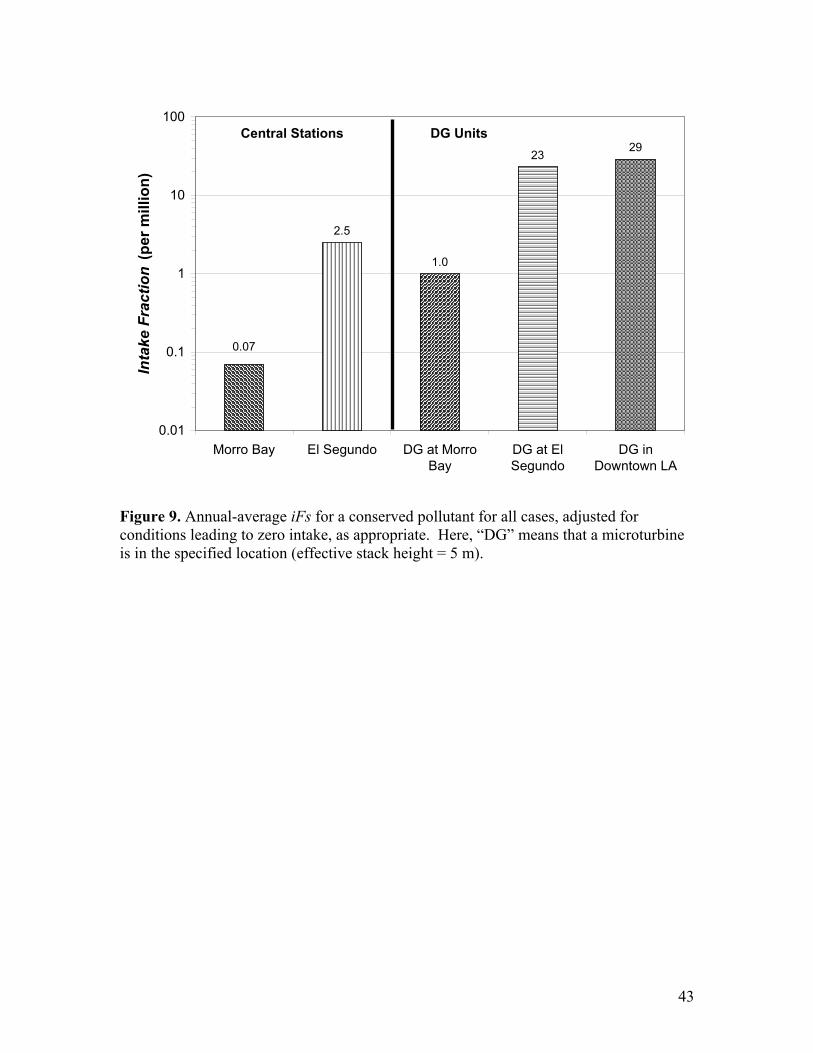
0.07

2923

1.0

2.5

0.01

0.1

1

10

100

Morro Bay El Segundo DG at MorroBay

DG at ElSegundo

DG inDowntown LA

Inta

ke F

ract

ion

(per

mill

ion)

Central Stations DG Units

Figure 9. Annual-average iFs for a conserved pollutant for all cases, adjusted for conditions leading to zero intake, as appropriate. Here, “DG” means that a microturbine is in the specified location (effective stack height = 5 m).

43

III.B.2 Key Factors Governing Intake Fraction for Conserved Pollutants There are many differences among the cases that influence the intake fraction. In

this section, we evaluate the relative influence of proximity (in terms of effective stack height), population and meteorological conditions (one determinant of persistence) on population exposures to air pollutants emitted by electricity generation sources. We do this by answering the question, what changes in these parameters are necessary to move from one case study result to another? The example we present starts with the case of the El Segundo Generating Station and is transformed one step at a time to the case of the microturbine at Morro Bay. Table 10 shows in which order the various elements were changed in this example.

Figure 10 compares the results of the base case (El Segundo central station) to intermediate, hypothetical cases where one element of the Morro Bay microturbine case is sequentially switched with the corresponding El Segundo element. First, meteorological conditions from Morro Bay are used in place of El Segundo’s. Operationally, this translates to changing mean wind speed from 3.7 to 2.1 m/s, the prevalence of onshore winds from 62% to 70% and the prevalence of each stability class to Morro Bay’s (see Table 6). These changes nearly double the intake fraction, with the decrease in wind speed accounting for most of the change.

When the substantially higher population density downwind of El Segundo is switched to Morro Bay’s lower value, the intake fraction decreases by over an order of magnitude. Since the intake fraction scales linearly with population density, this result is expected. 28 Increasing effective stack height from 244 and 297 m for the two El Segundo stacks to the Morro Bay effective stack height of 460 m reduces the intake fraction by 50%. However, comparing the intake fractions at either the 244/297 m or 460 m stack heights with the intake fraction associated with the DG effective stack height of 5 m demonstrates the importance of proximity in the vertical dimension and especially the order-of-magnitude difference in population intake between the two paradigms of electricity generation. The smaller change between ~ 250-300 m and ~ 450-500 m effective stack heights suggests that after a certain point, increasing stack height has marginal returns for reducing population intake. However, a more thorough investigation of the functional dependence of iF on stack height would be necessary to fully understand the relationship between these parameters.

28 The difference in population density downwind of El Segundo and Morro Bay is seen by comparing the distance-weighted, average density—1359 to 36 people/km2.

44

Tab

le 1

0. S

tep

that

a g

iven

par

amet

er w

as c

hang

ed in

mov

ing

from

the

case

of

El S

egun

do c

entr

al s

tatio

n to

mic

rotu

rbin

e at

Mor

ro B

ay.

El S

egun

doE

l Seg

undo

w/

Mor

ro B

ay M

et.

El S

egun

do w

/ M

orro

Bay

Met

. an

d P

op.

Mor

ro B

ayD

G a

t Mor

ro B

ay

Win

d sp

eed

üM

odal

win

d di

rect

ion

prev

alen

ceü

Atm

osph

eric

st

abil

ity

clas

s m

ixü

Pop

ula

tion

Dow

nwin

d po

pula

tion

dens

ity

ü

Pro

xim

ity

Stac

k he

ight

ü

(to

460m

)ü

(to

5m)

Met

. = m

eteo

rolo

gy

Pop.

= p

opul

atio

n

45

Key

iF

Fac

tors

Par

amet

er

Sequ

enti

al C

ase

Per

sist

ence

2.47

4.52

0.14

0.07

1.05

0.01

0.1

1

10

El Segundo El Segundo w/Morro Bay Met.

El Segundo w/Morro Bay Met.

And Pop.

Morro Bay DG at MorroBay

Inta

ke F

ract

ion

(per

mill

ion)

Figure 10. iF results from sequentially switching certain, key parameters, starting from the El Segundo central station case and moving to the DG at Morro Bay case for conserved pollutants. “Met” stands for meteorology (including wind speed and prevalence of modal wind direction and stability class) and “pop” for population. The other parameter that was changed was effective stack height. These cases were adjusted for conditions leading to zero intake, as appropriate.

46

III.B.3 Decaying Pollutant Results The results in Figure 11 show that the annual-average intake fractions for

formaldehyde, a decaying pollutant, are lower than for a conserved pollutant. The average reduction for all cases was 31%, with a range of 18 to 43%. Two patterns emerge when comparing the fractional reduction in iF for each case. First, intake fractions for the two Morro Bay cases decrease more than for the three cases located in the South Coast Air Basin. Second, intake fractions for the central station cases decrease more than for the DG cases. There are two likely causes for these patterns: 1) differences in the mass decay rate of the plumes; and 2) the relationship between who is exposed downwind and stack height.

Plume decay is governed by the exponential decay term, e-kx/U, and is the same for all cases emitting under the same conditions, i.e., with the same wind speed (U) and formaldehyde reaction rate (k). This means that plume decay is the same for the microturbine and central station located at Morro Bay; the cases located at El Segundo and downtown LA are also the same. For the cases at both Morro Bay and in the SoCAB, by the time the plume reaches 100 km downwind, approximately 2% of the mass remains; the mass remaining at distances of 1 and 10 km are also approximately the same for the two locations. This demonstrates that the differences in k and U of these cases counteract to produce roughly equal effect. Consequently, variation in plume decay does not cause the variation in iF observed.

The disparity in fractional reduction of iF can be explained by examining how the differences in distribution of downwind population and stack height relate to iF. Relative to a conserved species, intake fraction for a decaying pollutant emphasizes the population intake in the near-source region. Thus, one would expect to observe a greater reduction in the iF for a decaying pollutant in cases where population is distributed more evenly. The weighting of population near to the source (i.e., within 10 km) is much greater for the SoCAB cases than for Morro Bay, which explains why we observe greater fractional reduction for the Morro Bay cases.

Similar reasoning can account for the differences in fractional reduction of iF between DG and central station cases, where low stack height emphasizes the contribution of the population near to the source to iF. Again, comparing formaldehyde to a conserved species, the reduction in intake fraction for DG in downtown LA is the smallest since the population near to the source bears the proportionately largest burden in this case.

47

48

Figure 11. Annual-average iFs for a conserved pollutant and HCHO for all cases, adjusted for conditions leading to zero intake, as appropriate. HCHO reaction rate is slower in Morro Bay due to lower background OH concentration (Morro Bay is modeled with “rural’ while El Segundo is modeled with “moderate” background pollution).

igure 11. Annual-average iFs for a conserved pollutant and HCHO for all cases, adjusted for conditions leading to zero intake, as appropriate. HCHO reaction rate is slower in Morro Bay due to lower background OH concentration (Morro Bay is modeled with “rural’ while El Segundo is modeled with “moderate” background pollution).

ndoDG in

DowntownLA

0

5

10

15

20

25

30

Morro Bay DG at MorroBay

El Segundo DG at ElSegu

Inta

ke F

ract

ion

(per

mill

ion)

Conservedpollutant

HCHO

0.24 0.13

III.B.4 Cumulative Intake Fraction We calculated cumulative intake fractions versus downwind distance for the three

most prevalent stability classes — C, D and F — for both the central station and DG cases at El Segundo in order to elucidate the differences in distribution of intake between the two paradigms of electricity generation. 29 These results have not been adjusted for conditions leading to zero intake. Switching the downwind population density from the actual downwind distribution to the distance-weighted average reveals further information regarding distributional attributes of population intake. We also compare the results for conserved pollutants and for formaldehyde.

Figure 12 displays the results for conserved pollutants in stability class C (slightly unstable). Discontinuities in slope occur where our modeled population densities changed at county boundaries. For conserved pollutants, even distant populations can accumulate intake. The El Segundo cases use LA county population density out to 100 km (929 people/km2) and so the population intake continues to increase throughout. When more rural counties are reached beyond 100 km, the incremental population intake exhibits a plateau.

Only within the first five kilometers do the plots show a curve in incremental intake. This indicates the zone of most rapid vertical dispersion. While dispersion in the transverse direction decreases local ground-level concentrations, it increases the area impacted by the emissions. Consequently, only dispersion in the vertical direction changes cumulative population intake. The ultimate effect of vertical dispersion is to make the vertical extent of the plume uniform throughout the mixed layer; the more unstable the atmosphere, the earlier this condition is reached.

The curve of incremental population intake is convex for the DG cases. Since the plume is emitted at ground level, population intake accumulates rapidly, with the greatest slope occurring within the first 5 km from the source. As the plume becomes better mixed vertically, the slope falls off and then becomes constant after vertical mixing slows. Comparing the results from the DG cases in each stability class (Figures 12-14) confirms that vertical mixing is slower under the neutral and moderately stable conditions of D and F as compared to stability class C. The distance downwind before the population intake curves become linear is greater the more stable the atmosphere.

For the central station cases, the population intake curve within 5 km of the source is concave. Cumulative intake is small until the plume reaches the ground. From this position concentrations begin to increase rapidly, causing a rapid increase in the slope of the population intake curve.

Comparing the final values for the DG and central station cases, we see that the difference between them is greatest under moderately stable conditions, when the central station plume is separated from the ground and the DG plume remains close to the ground. Under slightly unstable conditions, the difference is least.

29 The results for Morro Bay and downtown LA show a similar pattern as for El Segundo.

49

0

5

10

15

20

0 20 40 60 80 100Distance Downwind, x (km)

Inta

ke F

ract

ion

(per

mill

ion)

DG at El Segundo

DG at El Segundousing ave.downwindpopulation density

El Segundo

El Segundo usingave. downwindpopulation density

Figure 12. Conserved pollutant iFs as a function of downwind distance for stability class C (slightly unstable) for El Segundo and a microturbine (“DG”) located at the same site, varying downwind population density from the actual to a distance-weighted average population density.

50

0

5

10

15

20

25

30

0 20 40 60 80 100Distance Downwind, x (km)

Inta

ke F

ract

ion

(per

mill

ion)

DG at El Segundo

DG at El Segundousing ave.downwindpopulation density

El Segundo

El Segundo usingave. downwindpopulation density

Figure 13. Conserved pollutant iFs as a function of downwind distance for stability class D (neutral) for El Segundo and a microturbine (“DG”) located at the same site, varying downwind population density from the actual to a distance-weighted average population density.

51

0.01

0.1

1

10

100

0 20 40 60 80 100Distance downwind, x (km)

Inta

ke F

ract

ion

(per

mill

ion)

DG at El Segundo

DG at El Segundousing ave.downwindpopulation density

El Segundo

El Segundo usingave. downwindpopulation density

Figure 14. Conserved pollutant iFs as a function of downwind distance for stability class F (moderately stable) for El Segundo and a microturbine (“DG”) located at the same site, varying downwind population density from the actual to a distance-weighted average population density.

52

Figure 15 displays similar results to Figure 12 except a decaying pollutant, formaldehyde, is considered rather than a conserved pollutant. In all cases, the slopes in each zone of population density are shallower, indicating that the concentrations are lower. Within the first twenty kilometers, the slopes and cumulative values are nearly equal, although consistently less, than those for conserved pollutants. At distances greater than twenty kilometers, the incremental intake is considerably less than that for conserved pollutants. This result indicates the diminished contribution of distant populations to total intake as a pollutant undergoes decay.

Figures 12-15 include traces that compare spatially resolved population density (at the county-level) with constant population density (at the same distance-weighted average value). Comparing these results from El Segundo provides further evidence of the relative importance of near-source population to total intake for the two paradigms of electricity generation. For distributed generation, the intake fraction is considerably higher for the spatially resolved distribution of population, as compared with the uniform population distribution. However, for the El Segundo central station case, in which the plume does not reach the ground until it has traveled some distance downwind, the effect of varying population density is much smaller in magnitude and variable in direction. These results indicate the importance of populations near to the source to population intake for ground-level releases and of more distant populations for elevated releases.

53

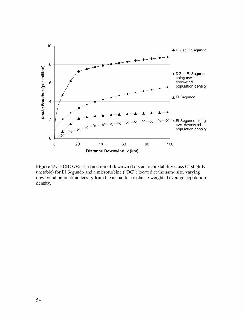
0

2

4

6

8

10

0 20 40 60 80 100Distance Downwind, x (km)

Inta

ke F

ract

ion

(per

mill

ion)

DG at El Segundo

DG at El Segundousing ave.downwindpopulation density

El Segundo

El Segundo usingave. downwindpopulation density

Figure 15. HCHO iFs as a function of downwind distance for stability class C (slightly unstable) for El Segundo and a microturbine (“DG”) located at the same site, varying downwind population density from the actual to a distance-weighted average population density.

54

III.B.5 Comparison to Previously Published Research This study extends previous research in several dimensions. On the particular

question of the ramifications of increased use of DG technologies to urban air quality, previous research has been limited to evaluating total mass emissions of DG versus central station plants into particular air basins or districts (Allison and Lents, 2002; Iannucci et al., 2000) or to simply compare emission factors (Greene and Hammerschlag, 2000). Such evaluations are limited in their ability to assess actual impacts on air quality as they do not account for pollutant transformations and interactions with background atmospheric concentrations. More importantly, they do not assess the impacts of air pollutant emissions on human exposure to those pollutants. Each of these studies considered the likelihood that closer proximity would lead to increased exposures, but did not quantify the issue for lack of an adequate analytical tool. To quote Allison and Lents: “The great difficulty…will be the development of an appropriate factor to account for the central-station to DG location and stack height differences” (Allison and Lents, 2002). We believe that the intake fraction is such a factor.

More generally, other researchers have assessed the intake fraction for pollutants emitted from large point sources (Smith, 1993; Lai et al., 2000; and Evans et al., 2002). Leveraging a study of exposure to primary particles emitted from 86 hypothetical coal-fired power plants in the US (Rowe, 1981), Smith was able to estimate the intake fraction from these plants to be 1 per million. Lai et al. (2000) did not look at power plants explicitly, but after extensive sensitivity analyses concluded that outdoor releases from elevated point sources would lead to intake fractions in the approximate range of 1 to 100 per million. Evans et al. (2002) report the results of a doctoral thesis (Wolff, 2000) that estimated intake fractions for a stratified random sample of 40 US coal-fired power plants. They found that the average iF for primary PM2.5 emissions was 2.2 per million, with a minimum of 0.25 and maximum of 6.3 per million. Taking into account that we limited our modeling domain to 100 km downwind (far less than Wolff, for instance), our central station iF results of 0.07 and 2.5 per million agree reasonably well with these previously reported values.

The agreement between our results and those of Wolff (2000) is noteworthy, especially because of the methodological differences. Wolff’s study provides a useful comparison for our central station cases, so we will explore the differences in our methods briefly here. Wolff used CALPUFF (EPA, 1995), a combination trajectory and Gaussian model, to estimate downwind concentrations within 100 km × 100 km grid cells in a total area of 1600 km × 2800 km encompassing the power plant. The model updates meteorological conditions from the nearest weather station as the plume travels downwind. It incorporates loss of PM2.5 by dry deposition. Finally, it uses average population density within the area of each grid cell.

Wolff’s model is more robust than ours in its treatment of such issues as plume meander, particle loss and time-varying meteorological conditions. There are also aspects of our models that are similar, such as the treatment of population heterogeneity (both within approximately the same grid spacing). Based on the differences, it is interesting to find that our simpler model agrees so well with the more complex one. The one more robust feature of our model is that we estimate concentration at 500 m intervals. This is especially important when considering releases from ground-level sources as this

55

study demonstrates that the contribution to population intake in the near-source region can be considerable.

The novel contribution of our study is the quantitative exploration of differences in exposure between the two paradigms of electricity generation, central station and distributed generation. Previous research has shown that differences in effective stack height are an important factor influencing intake fraction (Lai et al., 2000). Our research both extends this result to stack heights appropriate to distributed generation and confirms the more generic sensitivity analysis of Lai et al. (2000) through a series of case studies. III.B.6 Refined Analysis of Meteorological and Population Density Data

To determine the significance of our simplifying assumptions of meteorological and population parameters, we performed a supplementary evaluation of intake fraction for the same case study locations and technologies using more detailed representations of meteorological and population data. In the simplified analysis, we assumed constant mixing height and wind speed (at the harmonic means), only two wind directions (at the major and minor modes) and time-weighted stability class. For the refined analysis, we used a Latin hypercube sampling scheme to select randomly a substantial number of hours to represent a year of actual mixing height, wind speed and direction, and stability class data. In addition, the treatment of population density was refined. Instead of using constant county- or city-wide average values, in the refined analysis we utilized ArcView 3.2 GIS software (ESRI, 1999) to obtain census tract-level resolution. Further information about the methods and results of this assessment can be found in the Appendix.

Figure 16 displays results from both our original and supplementary analyses. The major exposure trends between case study locations and technologies are consistent between the two analysis approaches. The closer vertical proximity of DG units compared to central stations increases the intake fraction of conserved pollutants by approximately an order of magnitude. Additionally, the siting of an electricity generation unit in a densely populated region increases intake fraction by an order of magnitude as compared with rural siting.

These results demonstrate that the simplified treatment of meteorological and population parameters used in the original assessment sufficiently capture the magnitude and trends in intake fraction between the cases. However, the supplementary analysis revealed that higher-resolution meteorological and population data can be important if more accurate quantification of exposure impact is desired. The supplementary analysis also showed that spatially-resolved population data permits the apportionment of exposure burden to various subpopulations.

56

0.070

2.5

1.1

2329

0.060

5.43.7

31

55

0.01

0.1

1

10

100

Morro Bay El Segundo DG at MorroBay

DG at ElSegundo

DG inDowntown LA

Inta

ke F

ract

ion

(per

mill

ion)

Figure 16. Comparison of annual-average intake fraction between the original, modal wind direction model and the refined model for a conserved pollutant. The white bars are the results from the original, modal wind direction model. The black bars are results from the refined model.

57

III.C Intake Factor Results The intake factor (iFac) is an intake fraction normalized by the amount of

electricity delivered per mass of pollutant emitted. The goal in this section of the report is two-fold: 1) to estimate intake factors for existing microturbines and existing and new central stations and 2) to provide a preliminary estimate of an emission factor that new microturbines should meet to present no greater exposure hazard per unit of electricity generated (i.e., intake factor) than do central station plants. Table 11 and Figures 17-20 present the results of these assessments.

First, we compare iFacs for existing microturbines (i.e., those installed before the enactment of the CARB 2003 DG emission standard) and existing central station plants (i.e., Morro Bay and El Segundo). This comparison defines the baseline difference in intake factor between the two paradigms of electricity generation for units that are in operation today.

In addition to the existing central stations, new combined cycle turbines burning natural gas are also considered to complete the comparison of what DG technologies might displace if there is the shift in electricity generation paradigm that many predict. In terms of future capacity additions, especially in California, seemingly the only central station combustion technology with which DG technologies will be competing is combined cycle gas turbines. These plants are similar in many respects to the traditional central stations — fuel consumed, types of pollutants emitted, stack heights, siting preferences — but are more efficient and emit at rates comparable to or better than the most controlled existing central stations. 30 Thus, they provide a ‘best’ central station case for the comparison of population intake of atmospheric emissions.

Three pieces of data are required to assess combined cycle turbines: emission factors, thermal efficiency and intake fraction. We have already discussed the emission factors and thermal efficiency we use to characterize new combined cycle plants. To estimate intake fractions, we assume that the new combined cycle plants will be located at the same sites as the current central-station facilities at Morro Bay and El Segundo. Assuming similar stack characteristics, the iFs will be the same as for the real units. 31

Results of the comparison of intake factors for existing microturbines to existing and new central stations can be found in the “Base Case Intake Factors” section of Table 11 and are displayed in Figures 17 and 18. While it is true that DG technologies can be located anywhere, their distribution will be focused where there are electrical (and possibly heating and cooling) loads. Aside from pockets of energy-intensive industries that do not require large labor pools, the density of electricity consumption correlates well with population density in California (CEC, 2001a). Thus, to follow the most likely scenarios of DG deployment, the results for suburban and urban (downtown) DG should be compared against the typical central station siting of suburban or rural.

In general, for both PM2.5 and formaldehyde, comparisons between the various scenarios of DG siting and the central station cases reveal a one to four order-of-magnitude ratio in intake factor. The only exception is for a rurally sited microturbine

30 Assuming that regulations will require installation of control technologies such as selective catalytic reduction for NOx control. 31 Effective stack heights from combined cycle plants may be lower than for the central station cases we examined here due to higher conversion efficiencies reducing the waste heat emitted. However, for the assessment reported here, we have assumed that the effective stack height will be unchanged.

58

compared to El Segundo, where for both pollutants the intake factors are nearly equal. However, this comparison is on the margins of what most people expect will be the primary niche of DG technologies — servicing the commercial sector in populated zones. Thus, we find that existing, uncontrolled microturbines present a substantial exposure hazard compared to existing central station plants.

Given the inherent difference in intake fraction between the two paradigms of electricity generation, new DG technologies must be much cleaner than central stations in order to equalize population intake; how much cleaner depends on which central station technologies are compared. If one believes that new DG will displace the marginal electricity generator32, the correct comparison is to existing central station units. 33 If one believes that DG will only compete for capacity additions, then the correct comparison is to new combined cycle turbines. Results of both assessments are displayed in Table 11 and Figures 19 and 20.

For both PM2.5 and HCHO, the emission factors required for microturbines to achieve the intake factors of existing central stations are nearly equal to BACT for new central stations, i.e., an order of magnitude cleaner than the existing central station they would replace. In order to achieve the intake factors of new combined cycle turbines, microturbines will have to reduce PM2.5 and formaldehyde emissions by another order of magnitude, or ten times lower than currently required under BACT.

32 The marginal generator is the generator used to supply the final MW of demand, or the final generator on the load curve. 33 While we acknowledge that Morro Bay and El Segundo are both baseload plants and thus are unlikely to be the marginal generators that DG would displace, we limit our current assessment to those two plants. If one believes that the marginal generators will have higher emission factors than Morro Bay or El Segundo, then DG technologies could have correspondingly higher emission factors and still equalize the exposure burden. The opposite case can be made as well.

59

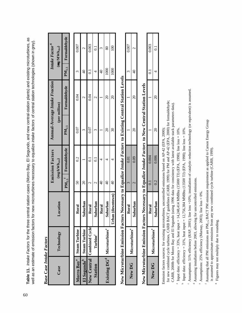
60

Bas

e C

ase

Inta

ke F

acto

rs

PM

2.5f

For

mal

dehy

deP

M2.

5F

orm

alde

hyde

PM

2.5

For

mal

dehy

de

Mor

ro B

aya

Stea

m T

urbi

neR

ural

500.

20.

070.

043

0.00

7

El S

egun

dob

Stea

m T

urbi

neSu

burb

an20

13

240

2

Rur

al2

0.1

0.07

0.04

0.1

0.00

3

Subu

rban

20.

13

24

0.1

Rur

al40

41

140

3

Subu

rban

404

2020

1000

80

Urb

an (

dow

ntow

n)40

430

2010

0010

0

New

Mic

rotu

rbin

e E

mis

sion

Fac

tors

Nec

essa

ry t

o E

qu

aliz

e In

take

Fac

tors

to

Exi

stin

g C

entr

al S

tati

on L

evel

s

Rur

al3

0.01

11

30.

007

Subu

rban

20.

0920

2040

2

New

Mic

rotu

rbin

e E

mis

sion

Fac

tors

Nec

essa

ry t

o E

qu

aliz

e In

take

Fac

tors

to

New

Cen

tral

Sta

tion

Lev

els

Rur

al0.

10.

004

11

0.1

0.00

3

Subu

rban

0.2

0.00

620

204

0.1

Em

issi

on f

acto

rs s

ourc

es:

for

exis

ting

mic

rotu

rbin

es, u

ncon

trol

led

emis

sion

s ba

sed

on A

P-42

(E

PA, 2

000)

;

for

new

com

bine

d cy

cle

turb

ines

, CA

RB

BA

CT

gui

delin

es (

CA

RB

, 199

9) f

or P

M a

nd A

P-42

(E

PA, 2

000)

for

for

mal

dehy

de;

C

AR

B, 2

000b

for

Mor

ro B

ay a

nd E

l Se

gund

o (u

sing

199

6 da

ta f

or c

onsi

sten

cy w

ith l

ates

t av

aila

ble

stac

k pa

ram

eter

s da

ta).

a In

put

data

: ef

fici

ency

= 3

3%, h

eat

inpu

t =

14,

248,

414

MM

Btu

(15

000

TJ)

(E

PA, 1

998)

; lin

e lo

ss =

10%

.b

Inpu

t da

ta:

effi

cien

cy =

31%

, hea

t in

put

= 1

2,75

6,38

4 M

MB

tu (

1350

0 T

J) (

EPA

, 199

8);

line

loss

= 1

0%.

c A

ssum

ptio

ns:

51%

eff

icie

ncy

(RA

P, 2

001)

; lin

e lo

ss =

10%

; in

stal

latio

n of

cat

alyt

ic r

educ

tion

tech

nolo

gy (

or e

quiv

alen

t) i

s as

sum

ed.

d A

ssum

ing

inst

alla

tion

befo

re 2

003,

allo

win

g fo

r un

cont

rolle

d em

issi

ons.

e A

ssum

ptio

ns:

25%

eff

icie

ncy

(Mar

nay,

200

3);

line

loss

= 0

%.

f A

ssum

ing

that

all

PM e

mis

sion

s ar

e PM

2.5;

BA

CT

PM

em

issi

on r

equi

rem

ent a

s ap

plie

d to

Car

son

Ene

rgy

Gro

up

is

assu

med

to

appr

oxim

ate

emis

sion

s fr

om a

ny n

ew c

ombi

ned

cycl

e tu

rbin

e (C

AR

B, 1

999)

.g

Figu

res

may

not

mul

tiply

due

to r

ound

ing.

New

DG

Mic

rotu

rbin

ese

New

DG

Mic

rotu

rbin

ese

Tab

le 1

1. I

ntak

e Fa

ctor

s fo

r the

thre

e ce

ntra

l sta

tion

case

s (M

orro

Bay

, El S

egun

do, a

nd n

ew c

entra

l-sta

tion

plan

ts) a

nd e

xist

ing

mic

rotu

rbin

es, a

s w

ell a

s an

est

imat

e of

em

issi

on fa

ctor

s fo

r new

mic

rotu

rbin

es n

eces

sary

to e

qual

ize

inta

ke fa

ctor

s of

cen

tral s

tatio

n te

chno

logi

es (s

how

n in

gre

y).

Cas

eT

ech

nol

ogy

Loc

atio

n

Em

issi

on F

acto

rsA

nn

ual

-Ave

rage

Int

ake

Fra

ctio

nIn

take

Fac

torg

(mg/

kW

hd

el)

(per

mil

lion

)(µµ

g/M

Wh

del

)

New

Cen

tral

S

tati

onC

omb

ined

Cyc

le

Tur

bine

c

Exi

stin

g D

Gd

Mic

rotu

rbin

ese

Figure 17. Intake factors for primary PM2.5 emissions from two existing and two new central stations and three existing DG cases (i.e., DG installed before the CARB 2003 DG emission standard). “CC” stands for combined cycle natural gas turbine; these units meet current BACT standards. “DG” is distributed generation, which are microturbines in the case of this study.

0.01

0.1

1

10

100

1000

10000

at MorroBay

DG at ElSegundo

DG inDowntown

LA

( µg i

nhal

ed/M

Wh d

el)

Morro Bay El Segundo New CC atMorro Bay

New CC atEl Segundo

DG

iFac

Existing and New Central Stations

Existing DG Units

61

0.001

0.01

0.1

1

10

100

1000

Morro Bay El Segundo New CC atMorro Bay

New CC atEl Segundo

DG at MorroBay

DG at ElSegundo

DG inDowntown

LA

iFac

( µg i

nhal

ed/M

Wh d

el)

Existing DG UnitsExisting and New Central Stations

Figure 18. Intake factors for primary HCHO emissions from two existing and two new central stations and three existing DG cases (i.e., DG installed before the CARB 2003 DG emission standard). “CC” stands for combined cycle natural gas turbine; these units meet current BACT standards. “DG” is distributed generation, which are microturbines in the case of this study.

62

0.01

0.1

1

10

New DG at Morro Bay New DG at ElSegundo

New DG at Morro Bay New DG at ElSegundo

Emis

sion

Fac

tor (

mg/

kWh d

el)

To equal iFac of existing central stations

To equal iFac of new combined cycle central stations

Figure 19. Estimate of PM2.5 emission factors necessary for newly installed DG to equal the iFacs of existing or new central stations.

63

0.001

0.01

0.1

1

New DG at Morro Bay New DG at ElSegundo

New DG at Morro Bay New DG at ElSegundo

Emis

sion

Fac

tor (

mg/

kWh d

el)

To equal iFac of existing central stations

To equal iFac of new combined cycle central stations

Figure 20. Estimate of HCHO emission factors necessary for newly installed DG to equal the iFacs of existing or new central stations.

64

III.D Summary of Results The intake fraction and intake factor appear to be useful metrics to compare the

potential for differential exposures to air pollutants emitted by the two paradigms of combustion-based electricity generation. In this assessment, we have explored the importance of many elements of the three key factors that influence the intake fraction. Proximity was evaluated in terms of effective stack height, persistence in terms of meteorology (e.g., wind speed and atmospheric stability) and pollutant decay, and population in terms of its distribution and density. For the conditions considered, the two factors that had the greatest relative impact on intake fraction were stack height and downwind population density, each contributing a one order-of-magnitude or larger effect. The distribution of downwind population was also an important factor, where short stack heights (i.e., from DG technologies) emphasized the contribution of the population near to the source to total population intake and tall stacks emphasized the more distant population’s contribution.

By contrast, persistence had a smaller effect over the range of conditions considered, only affecting the intake fractions by 30% to a factor of two. Wind speed had a plus or minus factor of two impact on intake fraction. A protective effect was seen for stable atmospheric conditions when pollutants were released from tall stacks and the opposite effect was observed for releases from short stacks. The atmospheric decomposition of primary formaldehyde emissions reduced the intake fraction by 30-50% for the cases explored here. Similar to the effect of short stacks, decaying pollutants emphasize population intake near to the source, whereas the intake of conserved pollutants can accumulate at great distances.

More robust sensitivity analyses are needed to verify these findings and the relative importance of the many factors that can affect intake fractions. Nevertheless, some confidence is gained by the agreement between the results of this study and similar ones identified in the previous two sections.

After accounting for the differences in efficiency, emission rates and line losses between the two paradigms of electricity generation, the intake factors for existing microturbines were one to four orders-of-magnitude higher than for the existing and new natural gas central stations considered in this study. In order to equalize the exposure burden (i.e., intake factor) of existing or new central station generation, new microturbine PM2.5 emission factors must either be equal to or an order-of-magnitude lower than new combined cycle EFs, respectively. For formaldehyde emissions, the necessary EFs for new microturbines are an order-of-magnitude or two lower than new combined cycle turbines. These requirements are a result of the inherent disadvantage that distributed generation has in terms of intake fraction. They pertain to microturbines in rural and suburban locations; if new microturbines are sited in downtown urban locations, the emission factors would have to be reduced even further. IV. Conclusions

Political and market leaders predict rapid growth in the market for DG in the United States and around the world (DOE, 2000; Allied Business Intelligence, 2002). Regulatory actors have recently begun to assess the significance of this expansion with regard to air quality and public health. Already, we know that electricity generation is a significant contributor to state and national emission inventories. In addition, recent studies have demonstrated that power plants impose significant direct human health impacts and monetary damages based on their emissions of criteria pollutants (e.g., Rabl

65

and Spadaro, 2000; Levy et al., 1999). Based on the findings of this preliminary study and on the assumption that the most mature DG technologies — i.e., those that are combustion-based — will capture much of the early market, there is reason to caution against an unmitigated embrace of DG and to continue investigations regarding the potential air quality and health impacts of DG technologies.

There are fundamental differences between the DG and central-station paradigm in the spatial association between where pollutants are emitted and where people are exposed. The closer proximity of DG technologies can increase the fraction of pollutants inhaled by an order of magnitude compared to our current central station approach. When considering that the likeliest siting of DG will be in areas of higher population density than for many central stations, population intake may be increased by another order of magnitude. These differences, expressed here through the intake fraction, place DG at a severe disadvantage if measured in terms of human exposure to atmospheric emissions.

With emission factors for DG technologies installed before 2003 often considerably greater than for the best-controlled central stations, the mass of pollutants inhaled by the exposed population normalized by the electricity delivered (i.e., intake factor) can be up to four orders-of-magnitude greater for DG compared to central stations. Despite uncertainty in the number and location of the existing stock of DG technologies, the preliminary findings of this research highlight the potential hazard these existing units present.

To ensure that the public health consequences of electricity generation do not become worse will require emission characteristics from new DG technologies that are much better than from central station facilities in order to make up for DG’s inherent intake fraction handicap. For PM2.5 emissions, DG emission factors will have to be an order-of-magnitude less than existing central stations in order to equal their exposure burden per unit of electricity delivered; the same ratio is necessary when comparing DG to new combined cycle gas turbines. For the case of formaldehyde, emission factors for new microturbines must be an order-of-magnitude or two lower than existing or new central stations, respectively, in order to equalize exposure burden.

The CARB emission standard requires emission factors from new DG to meet the level of BACT for central stations by 2007. However, equal mass emission rates do not imply equal air pollutant exposure impact. As evidenced by the above mentioned findings, the exposure burden from distributed generation technologies will remain significantly greater than for central stations unless additional emission factor reductions are made. Furthermore, the CARB emission standard only mandates limits on the emissions of four pollutants. Whether emissions of pollutants not expressly regulated will also be reduced is a matter of speculation. What is clear is that current DG emission factors for other pollutants of concern, such as benzene and formaldehyde, can impose significantly increased inhalation exposures due to their close proximity to downwind populations.

Using waste heat in combined heat and power applications can help mitigate the exposure increase by offsetting other emissions, but even the 30-40% efficiency gains will not account for the order-of-magnitude or greater difference in potential exposures, at least not on an individual unit basis. This study did not consider the system-wide effects of full-scale deployment of DG in CHP mode, which could have non-intuitive effects and remains an open issue for future research.

66

The specific results of this study reflect the particularities of the cases chosen. Nonetheless, these cases are at least indicative and at best representative of the spectrum of electricity generation facilities in California. Continued work in this area could improve the robustness of the conclusions through more elaborate treatment of several aspects of the assessment. Nevertheless, the scale of the effects observed and the elucidation of their underlying causes suggest that our broad findings may be true beyond the limits of the specific cases considered.

To date, regulatory policy for DG in California has focused on limiting mass emission rates to a level consistent with good central-station performance. However, even this level of performance could lead to increased population exposures to many pollutants. To be protective of public health, regulators should consider the potential for increased exposures if combustion-based DG technologies are sited in densely populated areas. This consideration would be especially relevant during the 2005 mid-course review of the emission standard. To that end, we have provided estimates of the emission factors necessary for new microturbines to equal the exposure potential of existing and new central station facilities. Additionally, our results should provide further impetus for regulators to promote ultralow-emitting technologies, such as fuel cells, or nonemitting technologies, such solar photovoltaics. A strong move in this direction would capture the many benefits of DG while leading to improvements in ambient air pollution and reductions in greenhouse gas emissions — a clean, distributed energy future. V. Recommendations

The research reported here demonstrates progress in understanding the implications of a shift in electricity generation from a system relying on large, central station power plants to one relying on distributed generation technologies. However, much work remains to better characterize and quantify the potential impacts. Refinements of certain aspects of our current model would yield improvements in its accuracy. Additional efforts could expand the scope of the current model in key dimensions. Furthermore, there are issues that would require a new modeling approach to achieve significant progress. The recommendations for future research are prioritized within these three categories.

This research used a case study approach to estimate annual-average intake fractions and intake factors for particular central stations in California and one DG technology. The results indicate the expected scale of intake fractions (iF) and intake factors (iFac) from these different modes of electricity generation. Increasing the number, type and locations of central station and DG technologies assessed using the same modeling approach would achieve a set of results more representative of the distribution of electricity generation facilities in California now and in the future. However, before evaluating many new sites, the accuracy of the current model should be improved with incremental refinements in the treatment of certain modeling parameters. Examples include adding dry and wet deposition as loss mechanisms for emitted pollutants, incorporating more complete emission factors for DG technologies as they come available, and identifying sources of mixing height data that are closer to the electricity generation units.

There are other important issues that would require a significant expansion of the current model to address. We believe that with a reasonable-scale effort the current model could be adapted to address secondary formation of nitrogen dioxide. This should be the highest priority near-term goal as NO2 was identified in the hazard ranking as the

67

pollutant with the greatest potential health risk and for its importance to air quality compliance. However, assessing the contribution of electricity generation to the formation of other secondary pollutants such as ozone is a more complex matter that would require an alternative modeling approach. For example, one might need to apply a Gaussian-style subgrid plume model within the framework of a trajectory or urban airshed model to accurately capture the combined complexities of atmospheric photochemistry and transport from localized sources.

Two issues with regard to dispersion modeling deserve high-priority attention. First, since DG technologies are likely to be sited in densely populated areas, better representation of dispersion through complex terrain is essential. Also, since short stacks and decaying pollutants both emphasize population intake in the region near the source, a better understanding of the concentration profile within a few kilometers, and especially within 500 meters, is important for accurately estimating population intake.

A more nuanced approach to time-varying rates of emission, downwind concentrations, breathing rates and population location (i.e., mobility), would provide a more realistic assessment of population exposure to air pollutants emitted from electricity generation. For instance, start-up and part-load conditions are known to cause substantially higher emission factors. These conditions, in addition to the maintenance of electricity generation units, can greatly influence peak and average downwind concentrations and, thus, exposures.

Finally, including a formal sensitivity and uncertainty analyses in subsequent evaluations would be an important enhancement to quantify the significance of each of the underlying parameters and the robustness of the results.

Four other research efforts that would expand the scope of the current modeling effort should be considered. First, expanding the modeling domain to include a regional estimate of population intake (i.e., beyond 100 km) is fundamental to assessing the full burden imposed by electricity generation units, especially central station plants. To address this need, one would need to adopt a trajectory model and additional meteorological data to track the plume as it meanders with changing wind speed and direction. CALPUFF is a modeling tool that could serve as a starting point for such an effort.

Second, the system-wide effects of full-scale DG deployment within an urban airshed are not addressed in the current model and could be non-intuitive. One approach to addressing this issue would involve an aggregation of the impacts of individual electricity generation units along with careful treatment of the emissions offsets that would occur with DG deployed in a CHP mode. Another approach would be to move to an urban airshed model where total emissions from all DG and offset sources could be spatially- and temporally evaluated, along with the effects of background concentrations and other parameters.

Third, our current research employs a dispersion model to conduct an exposure assessment. Leveraging the population intake results, one could extend this analysis to risk assessment end points. An assessment of cancer risk would be relatively straightforward; however, the evaluation of pollutants whose dose-response curves exhibit thresholds or nonlinear behavior would be considerably more complex. Finally, other sources of the same pollutants emitted by electricity generation could be evaluated to estimate cumulative personal exposure.

Our research has revealed a large exposure impact from shifting centralized electricity generation to distributed generation. However, our effort reflects exploratory

68

research of limited scope. The significance of electricity generation as a source of air pollutants and societal health impacts argues that additional research is warranted to refine and expand the efforts we have begun. While the distributed generation industry is still nascent, continued research along the directions outlined above is crucial and timely.

69

VI. References AB 2588. 1987. Air Toxics Hot Spots Information and Assessment Act of 1987.

Statutes of 1987. Health and Safety Code, Section 44300-44394. Ackerman T, Andersson G and Soder L. 2001. Distributed Generation: A Definition.

Electric Power Systems Research, 57: 195-204. Allied Business Intelligence. 2002. Major Expansion Ahead for Distributed Generation

On a Global Scale According to Allied Business Intelligence. http://www.alliedworld.com/servlets/Home accessed on 5/20/02.

Allison JE and Lents J. 2002. Encouraging Distributed Generation of Power That Improves Air Quality: Can We Have Our Cake and Eat It, Too? Energy Policy, 30: 737-752.

Atkinson R. 2000. Atmospheric Chemistry of VOCs and NOx. Atmospheric Environment, 34: 2063-2101.

Bennett DH, McKone TE, Evans JS, Nazaroff WW, Margni MD, Jolliet O, and Smith KR. 2002. Defining Intake Fraction. Environmental Science & Technology, 36(9): 206A-211A.

California Spatial Information Library. 2002. Census Tracts (1990, Shoreline-clipped). http://www.gis.ca.gov/ accessed on 7/14/02.

Capstone Turbine Corporation. 2002. photo from http://www.microturbine.com/applications/cogeneration.asp accessed on 9/27/02.

Capstone Turbine Corporation. 2003. Applications. http://www.microturbine.com/applications/ accessed on 3/14/03.

CARB. 1999. Guidance for Power Plant Siting and Best Available Control Technology. California Air Resources Board, Sacramento, CA. Issued September 1999, as approved July 22, 1999.

CARB. 2000a. 2000 Statewide Estimated Annual Average Emissions. California Air Resources Board, Sacramento, CA. http://www.arb.ca.gov/app/emsinv/emssumcat_query.php?F_DIV=0&F_YR=2000&F_AREA=CA accessed on 3/16/02.

CARB. 2000b. California Emission Inventory Data. California Air Resources Board, Sacramento, CA. http://www.arb.ca.gov/emisinv/emsmain/emsmain.htm accessed on 2/25/02.

CARB. 2001a. Staff Report: Initial Statement of Reasons for the Proposal to Establish a Distributed Generation Certification Program. California Air Resources Board, Sacramento, CA. Release date: Sept. 28, 2001, as approved Nov. 15, 2001.

CARB. 2001b. The 2001 California Almanac of Emissions and Air Quality. California Air Resources Board, Sacramento, CA. http://www.arb.ca.gov/aqd/almanac/almanac01/almanac01.htm accessed on 3/5/02.

CARB. 2002. Final Regulation Order: Establish a Distributed Generation Certification Program. California Air Resources Board, Sacramento, CA. As filed July 23, 2002. http://www.arb.ca.gov/regact/dg01/finreg.pdf accessed on Aug. 1, 2002.

CEC. 2001a. Environmental Performance Report of California’s Electric Generation Facilities. California Energy Commission, Sacramento, CA.

70

CEC. 2001b. California Gross System Electricity Production for 2001. California Energy Commission, Sacramento, CA. http://energy.ca.gov/electricity/gross_system_power.html accessed on Aug. 5, 2002.

CEC. 2001c. 2001 Database of California Power Plants. California Energy Commission, Sacramento, CA. http://www.energy.ca.gov/database/index.html#powerplants accessed on 2/25/02.

CEC. 2002a. Power Facility Licensing Cases Approved by the Energy Commission Since 1999. California Energy Commission, Sacramento, CA. http://energy.ca.gov/sitingcases/approved.html accessed on 8/5/02.

CEC. 2002b. Distributed Generation Strategic Plan. California Energy Commission, Sacramento, CA. As approved June 12, 2002.

CEC. 2002c. 1992-2001 Electricity Generation By Fuel Type. California Energy Commission, Sacramento, CA. http://www.energy.ca.gov/electricity/electricity_generation.html accessed on 8/13/02.

Christensen CS, Skov H, Nielson T and Lohse C. 2000. Temporal Variation of Carbonyl Compound Concentrations at a Semi-Rural Site in Denmark. Atmospheric Environment, 34: 287-296.

City of Los Angeles. 2001. City Of Los Angeles - Census 2000. http://www.lacity.org/pln/indexcpc.htm accessed on 3/5/02.

Clean Air Act. 1990. Section 112(f). Standards to Protect Public Health and the Environment.

Coastal Alliance. 2000. photo from http://plantexpansion.org/options.html accessed on 11/4/01.

Davidson GA. 1990. A Modified Power Law Representation of the Pasquill-Gifford Dispersion Coefficients. Journal of the Air & Waste Management Association, 40(8): 1146-1147.

Demerjian KL, Schere KL and Peterson JT. 1980. Theoretical Estimates of Actinic (Spherically Integrated) Flux and Photolytic Rate Constants of Atmospheric Species in the Lower Atmosphere. Advances in Environmental Science & Technology, 10: 369-459.

DOE. 2000. Office of Energy Efficiency and Renewable Energy, Office of Fossil Energy, United States Department of Energy, Washington, DC. Strategic Plan for Distributed Energy Resources. http://www.eren.doe.gov/der/pdfs/derplanfinal.pdf accessed on 8/5/02.

Energy Information Administration. 1999. Annual Energy Review 1998, United States Department of Energy, Washington, DC.

EPA. 1995. A User’s Guide for the CALPUFF Dispersion Model. EPA-454/B-95-006. Office of Air Quality Planning and Standards, United States Environmental Protection Agency, Research Triangle Park, North Carolina.

EPA. 1996. 1996 National Emissions Trends Database (Version 3). United States Environmental Protection Agency. http://www.epa.gov/ttn/naaqs/ozone/areas/plant/stcapln.htm accessed on 2/25/02.

EPA. 1998. Emission and Generation Resource Integrated Database (E-GRID98). United States Environmental Protection Agency. http://www.epa.gov/airmarkets/egrid/ accessed on 2/25/02.

71

EPA. 2000. Compilation of Air Pollutant Emission Factors, AP-42, Fifth Edition, Volume I: Stationary Point and Area Sources, Chapter 3.1: Stationary Gas Turbines. United States Environmental Protection Agency.

EPA. 2001. National Ambient Air Quality Standards. United States Environmental Protection Agency. http://www.epa.gov/airs/criteria.html accessed on 8/6/02.

EPA. 2002a. 1996 National Toxics Inventory. United States Environmental Protection Agency. http://www.epa.gov/air/data/ntimact.html accessed on 8/2/02.

EPA. 2002b. Technology Transfer Network, Support Center for Regulatory Air Models. United States Environmental Protection Agency. http://www.epa.gov/scram001/tt24.htm#mixing accessed on 3/10/02.

ESRI. 1999. ArcView GIS version 3.2. copyright 1992-1999. Environmental Systems Research Institute, Inc.

Evans JS, Wolff SK, Phonboon K, Levy JI and Smith KR. 2002. Exposure Efficiency: An Idea Whose Time Has Come? Chemosphere, 49(9): 865-1190.

Finlayson-Pitts BJ and Pitts JN. 1986. Atmospheric Chemistry. John Wiley and Sons. New York.

Friedfeld S, Fraser M, Ensor K, Tribble S, Rehle D, Leleux D, Tittel F. 2002. Statistical Analysis of Primary and Secondary Atmospheric Formaldehyde. Atmospheric Environment, 36: 4767-4775.

GAO. 2002. Air Pollution: Emissions from Older Electricity Generation Units. pub# GAO-02-709 Air Pollution. United States General Accounting Office.

Ghanandan R. 2002. California Electricity Workbook (version 3). Data compilation from various sources (unpublished).

Gifford FA. 1961. Use of Routine Meteorological Observations for Estimating Atmospheric Dispersion. Nuclear Safety, 2(4): 47-51.

Greene N and Hammerschlag R. 2000. Small and Clean is Beautiful: Exploring the Emissions of Distributed Generation and Pollution Prevention Policies. The Electricity Journal, 13(5): 50-60.

Iannucci J, Horgan S, Eyer J and Cibulka L. 2000. Air Pollution Emission Impacts Associated with Economic Market Potential of Distributed Generation in California. Prepared for the California Air Resources Board, Sacramento, CA.

IUPAC. 2001. Summary of Evaluated Kinetic and Photochemical Data for Atmospheric Chemistry, Web version December 2001. International Union of Pure and Applied Chemistry, Subcommittee for Gas Kinetic Data Evaluation. http://www.iupac-kinetic.ch.cam.ac.uk/summary/IUPACsumm_web0112.pdf accessed on 6/10/02.

Krewitt W, Hurley F, Trukenmuller A and Friedrich R. 1998. Health Risks of Energy Systems. Risk Analysis, 18 (4): 377-383.

Kyle AD, Wright CC, Caldwell JC, Buffler PA and Woodruff TJ. 2001. Evaluating the Health Significance of Hazardous Air Pollutants Using Monitoring Data. Public Health Reports, 116: 32-44.

Lai ACK, Thatcher TL and Nazaroff WW. 2000. Inhalation Transfer Factors for Air Pollution Health Risk Assessment. Journal of the Air & Waste Management Association, 50:1688-1699.

Layton DW. 1993. Metabolically Consistent Breathing Rates For Use In Dose Assessments. Health Physics, 64(1): 23-36.

72

Levy, JI, Hammitt JK, Yanagisawa Y and Spengler JD. 1999. Development of a New Damage Function Model for Power Plants: Methodology and Applications. Environmental Science and Technology, 33(24): 4364-4372.

Marnay C. 2003. Personal communication. Compilation of manufacturers performance-related data for DG technologies.

Marshall JD. 2002. Exposure to Motor Vehicle Emissions: An Intake Fraction Approach. Masters Project. Energy and Resources Group. University of California Berkeley.

Nazaroff WW and Alvarez-Cohen L. 2001. Environmental Engineering Science, John Wiley and Sons, New York.

NREL. 1995. Typical Meteorological Year 2. National Renewable Energy Laboratory, Boulder, CO.

OEHHA. 1999. Toxicity Criteria Database. Office of Environmental Health Hazard Assessment, California Environmental Protection Agency, Sacramento, CA. http://www.oehha.org/risk/chemicalDB/index.asp accessed on 8/6/02.

OEHHA. 2001a. Prioritization of Toxic Air Contaminants Under the Children's Environmental Health Protection Act. Office of Environmental Health Hazard Assessment, California Environmental Protection Agency, Sacramento, CA. http://oehha.ca.gov/air/toxic_contaminants/pdf_zip/SB25%20TAC%20prioritization.pdf accessed on 8/6/02.

OEHHA. 2001b. All Chronic Reference Exposure Levels Adopted by OEHHA as of December 2001. Office of Environmental Health Hazard Assessment, California Environmental Protection Agency, Sacramento, CA. http://www.oehha.org/air/chronic_rels/AllChrels.html accessed on 8/6/02.

OEHHA. 2002. Chronic Reference Exposure Levels (RELs). Office of Environmental Health Hazard Assessment, California Environmental Protection Agency, Sacramento, CA. http://www.oehha.ca.gov/air/chronic_rels/ accessed on 8/9/02.

Pasquill F. 1961. The Estimation of the Dispersion of Windborne Material. Meteorological Magazine, 90(1063): 33-49.

Platts Global Energy. 2002. photo from: http://www.platts.com/engineering/issues/Power/0107/0107pwr_itinplant.shtml accessed on 10/5/02.

Rabl A and Spadaro, JV. 2000. Public Health Impact of Air Pollution and Implications for the Energy System. Annual Review of Energy and Environment, 25: 601-627.

RAP. 2001. DR Emissions Rule Nov Draft, Appendix B. Regulatory Assistance Project. http://www.rapmaine.org. accessed on 2/9/02.

Riley WJ, McKone TE, Lai ACK, Nazaroff WW. 2002. Indoor Particulate Matter of Outdoor Origin: Importance of Size-Dependent Removal Mechanisms. Environmental Science and Technology, 36(2): 200-207.

Rowe MD. 1981. Human Exposure to Particulate Emissions from Power Plants. BNL-51305. Brookhaven National Laboratory. Upton, NY. As cited by Evans et al. 2002.

SB 1298. 1999. California Senate, Sacramento, CA. http://www.arb.ca.gov/regact/dg01/appa.pdf accessed on 8/5/02.

Scheible M. 2002. Deregulation in California: What Does/Did It Mean for Air Quality. Presentation at the Haagen-Smit Symposium. California Air Resources Board. Lake Arrowhead, CA. April 10, 2002.

73

Scorecard. 2002a. Risk Assessment Value Availability. http://www.scorecard.org/chemical-profiles/def/assess_rav.html accessed on 3/14/02.

Scorecard. 2002b. Scorecard's Preferred Sources for Risk Assessment Values. http://www.scorecard.org/chemical-profiles/def/rav_priority.html accessed on 3/14/02.

Seinfeld JH and Pandis SN. 1998. Atmospheric Chemistry and Physics: From Air Pollution to Climate Change. John Wiley and Sons. New York.

Smith KR. 1993. Fuel Combustion, Air Pollution, and Health: The Situation in Developing Countries. Annual Review of Energy and the Environment, 18: 529-566.

Turner DB. 1994. Atmospheric Dispersion Estimates: An Introduction to Dispersion Modeling, 2nd Edition. Lewis Publishers. Ann Arbor, MI.

Union Gas. 2002. Chemical Composition of Natural Gas. http://www.uniongas.com/NaturalGasInfo/AboutNaturalGas/composition.asp accessed on 3/27/02.

Wolff SK. 2000. Evaluation of Fine Particle Exposures. Health Risks and Control Options. Doctoral Thesis. Department of Environmental Health, Harvard School of Public Health, Cambridge, MA. As cited by Evans et al., 2002.

74

VII. Glossary of Terms, Abbreviations, Units of Measure and Symbols

Terms and Abbreviations

AP-42 compilation of emission factors maintained by the US Environmental Protection Agency

AQMD air quality management district

atmospheric stability condition of the atmosphere governing rate of vertical mixing

BACT best available control technology

baseload power plant that is operated continuously, emitting pollutants at a constant rate

calms atmospheric condition in which wind speed is below detection limit of monitoring instrument

CARB California Air Resources Board

CEC California Energy Commission

central station large power plant used to provide electricity to the transmission and distribution network

CO carbon monoxide

combined cycle power plant that uses a turbine plus a steam generator to improve thermal conversion efficiency

CHP combined heat and power; electricity generation system that uses waste heat for beneficial purpose

conserved (pollutant/species) not removed from the air in an urban basin, except by air flow

control technology method of reducing pollutant emissions from a source

criteria pollutant air pollutant whose ambient concentrations must be maintained below the National Ambient Air Quality Standards established by the US Environmental Protection Agency

cumulative intake sum of air pollutant mass breathed by all members of an exposed population

de minimus below a minimum threshold for regulatory concern

decaying (pollutant/species) removed from urban air by a transformation process

demand-side resources any strategy, method or technology to reduce demand for electricity; e.g., energy conservation or increased energy efficiency

75

DER distributed energy resources; supply- and demand-side distributed electricity resources

DG distributed (electricity) generation; generation near the place of use

dispersion spreading of contaminants from regions of high concentration to regions of low concentration

distribution network system for transmitting lower-voltage electricity from sub-stations (which are connected to the transmission network) to sites of use

district air quality management district

DOE (United States) Department of Energy

EF emission factor; mass of pollutant emission per unit of activity, e.g., per heat input or electricity output

effective stack height height above ground at which pollutants are effectively emitted, accounting for both the physical stack height and plume rise

efficiency proportion of thermal energy in fuel converted to electricity in a power plant

El Segundo El Segundo Generation Station, geographically located in El Segundo, a small city (population 16,000) west of Los Angeles, CA

emission rate mass of pollutant emitted per unit time

EPA (United States) Environmental Protection Agency

inhalation exposure average pollutant concentration inhaled times the duration of the encounter with that concentration

Gaussian plume model mathematical representation of the pollutant concentration profile downwind of a localized source

HAPs hazardous air pollutants; a list of 188 pollutants designated in the Clean Air Act and maintained by the US Environmental Protection Agency

harmonic mean reciprocal of the average of reciprocals

hazard ranking / index measure of the relative degree of hazard posed by exposure to a particular pollutant

HCHO formaldehyde

iF intake fraction, proportion of pollutants emitted from a source inhaled by exposed population

iFac intake factor, equal to the product of the intake fraction times an emission factor

76

incremental intake contribution to the population intake per unit distance downwind of a source

inhalation unit risk factor a type of inhalation cancer potency factor; the probability of a person contracting cancer as a result of constant exposure to an ambient pollutant concentration of one microgram per cubic meter over a 70-year lifetime

inhalation cancer potency factor an estimate of a chemical's likelihood to cause cancer from inhalation

intake quantity of an air pollutant inhaled

inversion layer region of the atmosphere where the temperature rises with height

LA Los Angeles

line loss loss of electric power during transmission from the site of generation to the site of use

loss mechanism means of pollutant removal other than air flow, e.g. by chemical reaction

MEI maximally exposed individual

meteorological conditions mixing height, wind speed and direction, and atmospheric stability prevailing over some time at a particular location

microturbine a small-scale electricity generation technology that is based on aircraft engine turbo-chargers and uses natural gas as a fuel

mixing height distance between the ground and the base of an inversion layer where pollutants mix rapidly

modal wind direction wind direction that occurs most commonly

Morro Bay Morro Bay Power Plant, geographically located in Morro Bay, a small city on the central California coast in San Luis Obispo county

NAAQS National Ambient Air Quality Standards

NO2 nitrogen dioxide

NO3 nitrate radical

no-threshold, dose-response health hazard model of a pollutant that includes a finite risk for all exposures, no matter how small

NOx nitrogen oxides (generally NO + NO2)

NREL (United States) National Renewable Energy Laboratory

77

OEHHA (California) Office of Environmental Health Hazard Assessment

offshore wind direction from land to sea

OH• hydroxyl radical

onshore wind direction from sea to land

photolysis chemical reaction initiated by the absorption of a photon of light

plume downwind zone from a localized pollution source over which pollutant levels are elevated because of the source

plume rise extent to which a plume emitted with momentum or buoyancy moves upward relative to its emission height

PM2.5 particulate matter smaller than 2.5 micrometers in aerodynamic diameter

point sources air pollution sources that have small spatial extent (relative, e.g., to the size of a city)

population density number of people residing in a zone per unit land area, e.g., people per square kilometer

population intake cumulative pollutant intake by all members of an exposed population

prevailing wind direction synonymous with modal wind direction, or, the wind direction that occurs most commonly

primary pollutant air contaminant directly emitted from source

REL reference exposure level; concentration that poses no significant health risk from indefinite exposure

secondary pollutant air contaminant formed by chemical reactions in the atmosphere

SoCAB South Coast Air Basin

stability class one of six categories of atmospheric stability, as defined by Pasquill (1961)

stack height physical height of exhaust chimney from air pollution source

steam turbine technology for generating electricity that involves the expansion of compressed steam through a turbine

threshold maximum level of pollutant exposure or intake that would cause no adverse health effects

TMY2 Typical Meteorological Year 2 data set published by NREL (1995)

78

trajectory model method of accounting for the impact of an air pollution source on the downwind area by tracking the movement of air parcels

transmission network part of the electrical grid that transports electricity from generators along high voltage power lines to sub-stations and the distribution network

transverse direction direction in the horizontal plane normal to the prevailing wind flow

VOC volatile organic compound

well-mixed possessing uniform concentrations of pollutants

zenith angle angle between the vertical and the direction of the sun

Units of Measure

µg microgram; 10-6 grams

µm micrometer, 10-6 meters

d day

g gram

GW gigawatt; 109 watts

h hour

hp horsepower

kg kilogram; 103 grams

km kilometer; 103 meters

kW 103 watts

kWh kilowatt-hour

lbs pound

m meter

mg milligram; 10-3 grams

MMBtu million British thermal units

MW megawatt; 106 watts

s second

y year

79

Symbols Used in Equations

π pi

σx dispersion parameter in the downwind direction (m)

σy dispersion parameter in the transverse direction (m)

σz dispersion parameter in the vertical direction (m)

C concentration (g m-3)

Cc concentration of a conserved species (g m-3)

Cd concentration of a decaying species (g m-3)

Ε steady-state emission rate of a pollutant from a source (g s-1 or g h-1)

EF emission factor (e.g., mg per kWh)

HE effective stack height of an emission source (m)

I electric current

iF intake fraction

iFac intake factor (e.g., mginhaled per kWhdel)

iFc intake fraction of a conserved pollutant

iFd intake fraction of a decaying pollutant

k decay constant (s-1)

kWhdel kilowatt-hour of electricity delivered to the place of use

M mixing height (m)

n index for the number of reflections in the Gaussian plume model

P population density (people m-2)

Pe electric power

Ph rate of production of heat energy

QB breathing rate (m3 h-1)

R electrical resistance

U wind speed (m s-1)

V voltage

W width (m)

x downwind distance (m)

y distance in the transverse direction (m)

80

Appendix This appendix documents the methods and results of a supplemental evaluation of

the air pollutant exposure implications of a shift toward distributed electricity generation. In this portion of the study, a more detailed treatment of intake fraction modeling inputs was implemented with the goal of obtaining more precise results. The same case study locations and technologies were analyzed as those reported in the body of the report, but the heterogeneity in meteorological conditions and population distribution was more thoroughly assessed to examine their effects on the results. Specifically, a Latin hypercube sampling scheme was used to select a subset of hours to represent a year of mixing height, wind speed and direction, and stability class conditions, while ArcView 3.2 GIS software (ESRI, 1999) was used to gain population data resolution on the census tract level.

A.I. Methods

The case study locations and electricity generation technologies used in this follow-up analysis were described in section II.A of the report, with data relevant to air quality modeling given in Tables 4 and 5. The following subsections briefly summarize the analysis methods, with notes on all adjustments made for this reassessment.

A.I.A Gaussian Plume Model for Conserved Pollutants The downwind pollutant concentrations from the electricity generation sources

were modeled using the standard Gaussian plume equations described in section II.C.1.a. Again, the assessment of downwind concentration was limited to within 100 km, and electricity generation units were assumed to operate in a baseload capacity. The equation for time-average, ground-level, downwind concentration, C, of a steadily-released, conserved pollutant, incorporating a slender plume approximation and reflection at the ground and the base of the mixing height, is

(A1)

( ) ( )

+−+

−−

−= ∑∑

==

20

02

220

02

2

2

2

22exp

22exp

2exp

n z

E

n z

E

yzy

HnMHnMyU

ECσσσσπσ

where E is the steady-state emission rate of a pollutant from the source (g s-1), σy and σz are dispersion parameters in the transverse (y) and vertical (z) directions (m), respectively, U is the wind speed (m s-1), HE is the effective stack height of the emission source accounting for plume rise (m), x and y are the downwind and lateral distances, respectively, M is the mixing height (m) and n is an index for the number of reflections. The dispersion parameters were modeled using the modified power law form σ = axb+clnx, where a, b, and c are empirical parameters based on the original Pasquill-Gifford parameters (Pasquill, 1961 as modified by Gifford, 1961) as modified by Davidson (1990). The same assumptions of constant meteorological conditions within the transport time of the plume and perfect pollutant reflection at the system boundaries have been invoked.

81

A.I.B Meteorological Parameters Hourly measurements of mixing height, wind speed and direction, and stability

class were used directly in the Gaussian plume model to calculate concentrations. To account for the effects of daily and seasonal weather patterns, a Latin hypercube sampling scheme was implemented to select a stratified random sample of hours to represent a year. The year was divided into 219 groups of eight consecutive hours over five consecutive days (e.g., 1-8 AM, January 1-5). One hour was selected randomly from each of the 219 groups. The analysis was conducted for each of the 219 hours so selected. The annual average result was obtained by taking the arithmetic mean of the model output results for this representative set of hours. A.I.B.1 Mixing Height

For mixing height, the EPA Support Center for Regulatory Air Models data (EPA, 2002b) for Oakland were used for all cases. An average over the years 1984 to 1991 was taken for each daily AM or PM mixing height data point. As designated by the data set, the AM mixing height value was selected for hours between 10 PM of the day before and 9 AM (inclusive), while the PM value was used between 10 AM and 9 PM. When mixing height was lower than the effective stack height, all downwind concentrations of the pollutant were assumed to be zero. A.I.B.2 Wind Speed and Direction

Wind speed and direction were obtained from the National Renewable Energy Laboratory’s (NREL) Typical Meteorological Year 2 (TMY2) data set (NREL, 1995). As in the original assessment, data from the Santa Maria monitoring station were used for Morro Bay, while data from Los Angeles were used for both El Segundo and downtown LA. The wind speeds provided by these data sets were obtained for each of the 219 randomly selected hours. As described in section II.C.2.b, hours with zero measured wind speed were counted and reported as calms. However, these hours were not used in this evaluation because the Gaussian plume equations do not apply to calm conditions. Concentrations during calm hours may potentially be greater than during the hours being modeled. Of the 219 hours selected for the analysis, 9% and 5% of hours at Morro Bay and El Segundo/downtown LA, respectively, were calms. These values agree reasonably well with the annual prevalence of calms in the full data set: 7% and 4% at Santa Maria and Los Angeles, respectively.

Wind direction, although reported to the nearest 10°, was grouped into the closest 30° bin for ease of evaluation. The result for each of the 219 hours was one of twelve possible wind directions aligned to start at N 30° E. A.I.B.3 Atmospheric Stability Class

Atmospheric stability for each hour of the year had been determined for the initial assessment (see section II.C.2.c) by applying the Pasquill classification system (Pasquill, 1961) with necessary translations to the TMY2 data. The stability class for each of the 219 randomly selected hours used in this follow-up evaluation was drawn from this same data set.

82

A.I.C Population Parameters As stated in section II.C.3, the assessment of population exposures to air

pollutants requires two important factors relating to the exposed population: the breathing rate and number of exposed people. The lifetime average breathing rate of 12 m3/d (Layton, 1993), which accounts for differences by age and gender, was not changed from the original study. However, heterogeneity in downwind population was considered in substantial detail.

Census tract-level population density was utilized in place of county- or city-level estimates to better capture spatial variability. Shoreline-clipped 1990 census tracts (in an Albers Equal Area projection, North American Datum, 1927) were obtained from the California Spatial Information Library (2002) for processing by ArcView 3.2. Demographic information, including population density, was included in the data set.

The three case study locations were placed on the map according to their coordinates listed in Table A1. Radiating lines representing wind direction were added to each location at 30° intervals, starting at N 30° E and extending a length of 100 km. These radiating lines were converted to points designating where population density information was required for the model integration. The points were evenly spaced at 0.5 km intervals to match the numerical integration scheme chosen for the original study and repeated in the reevaluation. The demographic data associated with the census tracts was then spatially joined to the points, and exported as a database. Figures A1 and A2 show on two different scales the case study locations with census tracts and analysis points.

83

Table A1. Case study locations.

Case StudyLocation

Longitude(decimal degrees)

Latitude(decimal degrees)

El Segundo -118.4231 33.9106Morro Bay -120.8528 35.3708Downtown LA -118.3196 33.9403

84

Figure A1. Electricity generation locations with points at 0.5 km intervals radiating in twelve directions. Census tracts in the background are shaded by population density classified by natural breaks.

85

Figure A2. Zoom in on El Segundo and downtown LA with points at 0.5 km intervals radiating in twelve directions. Census tracts in the background are shaded by population density classified by natural breaks.

86

A.I.D Intake Fraction Calculation To repeat the assessment of the population intake of pollutants associated with

specific electricity generation techniques and locations, an annual-average intake fraction was calculated for each case study. Here, the annual-average intake fraction is the average of all intake fractions corresponding to the 219 random hours. The method of Lai et al. (2000) was employed with the same assumptions of unbounded crosswind plume spread and constant population density in the transverse direction (see section II.D.2.a), yielding the following expression of intake fraction (iF):

(A2) ( ) ( )

dxHnMHnMP

UQ

iFX

n z

E

n z

E

z

B ∫ ∑∑

+−+

−−=

==

max

0

20

02

220

02

2

22

exp2

2exp

2σσσπ

where P is the population density (persons m-2) and QB is the individual breathing rate (m3 s-1 person-1). The limit of integration is 0 to xmax = 100 km in the x-direction.

Assuming constant population density in the transverse direction introduces some uncertainty owing to lateral plume spread downwind. The merit of this assumption may be further diminished by the census tract-level resolution of population density. However, since the twelve wind directions were chosen without regard to specific downwind populations, population density off-vector at a given downwind distance is not expected to be systematically different than that on-vector. Therefore, this assumption may contribute to imprecision in our estimates, but not contribute to inaccuracy.

A.I.E Environmental Justice Analysis

Population intake is the sum of individual intakes over a specific population. For the main portion of this report, the population of interest was defined as all exposed persons within 100 km of the source. One aspect of environmental justice is concerned with how environmental insults are distributed among different demographic groups. For the purposes of a preliminary analysis of environmental justice concerns regarding electricity generation, we divided the exposed population into two subpopulations: white and nonwhite. The sum of intakes by white and nonwhite subpopulations equals the total population intake. Similarly, the sum of white and nonwhite intake fractions equals the total population intake fraction. Dividing the nonwhite intake fraction by the total population intake fraction, the proportional intake burden of nonwhite people can be determined. This exploratory analysis of intake fraction apportionment by race employed the original modal wind direction modeling scheme described in the body of the report but inserted census tract-level population density data in place of the overall population density to calculate nonwhite intake fractions.

87

A.II. Results and Discussion

A.II.A Annual-Average Intake Fraction Annual-average intake fraction is used to compare differences in population

exposure to air emissions between case study locations and technologies representing several electricity generation schemes. Conserved pollutant intake fraction results for each case are presented in Figure A3. Note that the results are applicable to any conserved pollutant since no pollutant-specific adjustments were made.

A comparison of differences in the magnitude of the intake fraction between pairs of cases reveals two major patterns. First, for the same location, lowering stack height from a central station level to a typical DG level increases the intake fraction by approximately an order of magnitude. The closer vertical proximity of the DG stack to the population leads to higher intake due to higher ground-level concentrations. This is the same trend revealed by the original study and discussed in sections III.B.1 and III.B.2. Comparing differences between locations, the intake fraction at El Segundo is at least an order of magnitude greater than the corresponding intake fraction at Morro Bay for both technologies. Further increases in intake fraction occur for a DG unit in downtown LA compared to a DG unit in Morro Bay or El Segundo. Again, this is the same trend discovered in the original assessment and discussed in sections III.B.1 and III.B.2.

88

0.060

5.43.7

31

55

0.01

0.1

1

10

100

Morro Bay El Segundo DG at MorroBay

DG at ElSegundo

DG inDowntown LA

Inta

ke F

ract

ion

(per

mill

ion)

Figure A3. Annual-average intake fractions for a conserved pollutant using the refined model. Note logarithmic scale.

89

A.II.B Population Distribution Analysis While the same qualitative patterns of exposure to air emissions for various

electricity generation locations and technologies have been substantiated by this supplementary assessment, changes in the detailed intake fraction estimates from the original to the refined study merit exploration. To begin, variation between population data inputs for the two assessments is examined. This exploration will provide hypotheses useful for subsequent interpretation and comparison of the final results from the original to the refined assessment in section A.II.C.

Since intake fraction scales linearly with population, the change in population data is a first indicator of how the refined calculations compare with the original estimates. For DG units, the short stack height creates high ground level pollutant concentrations near the source, making the near-source representation of population distribution very important. In contrast, a plume from a much taller central station stack does not reach the ground near the source, making the accurate representation of population data farther downwind more important.

Figure A4 depicts the original (county-average) and refined (census tract-level) Morro Bay population data inputs for the modal wind direction (300°). The very high census tract population densities near the source are not captured by the county average used in the original assessment. This difference suggests that the refinement will yield a significantly higher intake fraction for the DG unit at Morro Bay than the original estimate. Similar or fractionally lower tract level population densities compared to the county average farther downwind suggest that the intake fraction predicted by the refined model for the central-station case will be slightly lower than that predicted by the original model.

Downwind from El Segundo and downtown LA, census tract-level population densities are generally higher than county-average data. This trend is true, both near the source and further downwind, suggesting that intake fraction calculated by the refined model will be consistently higher than that calculated by the original model for the central station and the DG units. Population data inputs for the El Segundo and the downtown LA modal wind direction (250°) are displayed in Figures A5 and A6.

90

����������������������������������������������������������������������������������������������������������������������������������������������������������������������������������������������������������������������������������������������������������������������������������������������������������������������������������������������������������������������������������������������������������������������������������������������������������������������������������������������������������������������������������������������������������������������������������������������������������0

250

500

750

1000

1250

0 10 20 30 40 50 60 70 80 90 100

Distance Downwind (km)

Popu

latio

n D

ensi

ty (p

erso

ns/k

m2 )

County-average data

Census tract data

Figure A4. Population data inputs for the Morro Bay modal wind direction. County-average data (gray line) were used in the original model. Census tract data (black triangles) were used in the refined model.

91

��������������������������������������������������������������������������������������������������������������������������������������������������������������������������������������������������������������������������������������������������������������������������������������������������������������������������������������������������������������������������������������������������������������������������������������������������������������������������������������������������������������������������������������������������������������������������������������������������������������������

0

2000

4000

6000

8000

10000

0 10 20 30 40 50 60 70 80 90 100

Distance Downwind (km)

Popu

latio

n D

ensi

ty (p

erso

ns/k

m2 )

Census tract data

County-average data

Figure A5. Population data inputs for the El Segundo modal wind direction. County-average data (gray line) were used in the original model. Census tract data (black triangles) were used in the refined model.

92

�����������������������������������������������������������������������������������������������������������������������������������������������������������������������������������������������������������������������������������������������������������������������������������������������������������������������������������������������������������������������������������������������������������������������������������������������������������������������������������������������������������������������������������������������������������������������������������������������������������������

0

2000

4000

6000

8000

10000

0 10 20 30 40 50 60 70 80 90 100

Distance Downwind (km)

Popu

latio

n D

ensi

ty (p

erso

ns/k

m2 )

Census tract data

County-average data

Figure A6. Population data inputs for the downtown LA modal wind direction. County-average data (gray line) were used in the original model. Census tract data (black triangles) were used in the refined model.

93

A.II.C Annual-average Intake Fraction Comparison With these indications of how the intake fraction is likely to change from the

original modal wind direction model to the refined model, a quantitative comparison can now be made. Figure A7 depicts the conserved pollutant intake fraction results for both the original study and the reanalysis.

For all cases, the trends expected from the population data refinements were correct. Intake fraction predicted by the refined model was greater than the intake fraction of the original model for all cases except the central station at Morro Bay. As expected, these increases varied in their relative scale, with the largest increase occurring for a DG unit at Morro Bay. Nevertheless, the complexity of these changes merits further analysis of how the refinements in meteorological and population data inputs altered the quantitative results.

The simplest way to evaluate the effect of higher-resolution population data alone is to use the refined population data in the original modal wind direction model. If the results of this third modeling scenario are similar to the results of the refined model, then population can be implicated as the major driver of the differences between the original and refined results. Figure A8 presents intake fraction results from all three modeling scenarios. From this figure, it appears that the refined population density data is indeed the key factor controlling the change in results at El Segundo and downtown Los Angeles. In these locations the results from the refined model and the third modeling scenario vary by only 25% for the El Segundo central station and by less than 10% for the El Segundo and downtown LA DG units. At Morro Bay, where the results vary by more than 30%, the influence of using higher-resolution population data is less clear.

94

0.070

2.5

1.1

2329

0.060

5.43.7

31

55

0.01

0.1

1

10

100

Morro Bay El Segundo DG at MorroBay

DG at ElSegundo

DG inDowntown LA

Inta

ke F

ract

ion

(per

mill

ion)

Figure A7. Comparison of annual-average intake fraction between the original, modal wind direction model and the refined model for a conserved pollutant. The white bars are the results from the original modal wind direction model. The black bars are results from the refined model.

95

0.070

2.5

1.1

2329

0.060

5.43.7

31

55

0.040

6.8

1.6

3350

0.01

0.1

1

10

100

Morro Bay El Segundo DG at MorroBay

DG at ElSegundo

DG inDowntown LA

Inta

ke F

ract

ion

(per

mill

ion)

Original Modal Wind Direction Model

Refined Model

Modal Wind Direction Model with Refined Population Data

Figure A8. Comparison between three modeling scenarios of annual-average intake fraction for a conserved pollutant.

96

The observation that the intake fraction results from the refined model are not as similar to the third modeling scenario for Morro Bay as they are for El Segundo and downtown Los Angeles indicates that meteorological refinements may play a larger role in driving the differences at Morro Bay. One qualitative explanation can be made by comparing the Santa Maria wind histogram (Figure 6) to the Los Angeles wind histogram (Figure 5). A second modal wind direction is less obvious at Santa Maria than at Los Angeles, implying that the simplified representation using bimodal winds in the original model causes more inaccuracy at Morro Bay than at El Segundo or downtown LA. Therefore, a higher degree of refinement was achieved by the supplementary assessment for Morro Bay than for El Segundo or downtown LA because in LA there was a better chance that the 219 randomly selected hours fit into the primary or secondary mode used by the original model. Greater effects of refinement may explain the higher degree of variability between the refined and third scenario modeling results for Morro Bay compared to El Segundo or downtown LA. However, whether intake fraction would increase or decrease due to this effect is not immediately clear, and is a subject that would require further study.

A.II.D Environmental Justice Analysis The intake fraction attributable to nonwhite people as a portion of the overall

intake fraction ranges from 9% to 69% depending on case study technology and location. Figure A9 presents the nonwhite portion of intake fraction estimated for each case. For comparison, the nonwhite portion of the population in the census tracts within 100 km of the source in the modal wind direction is also reported.

Comparing downwind population racial demographics and intake fraction apportionment by race indicates a disproportionate exposure burden on nonwhite people for the El Segundo and downtown Los Angeles cases. In the most extreme example, for the downtown Los Angeles DG unit, 32% of the exposed population is nonwhite, yet this population group receives 69% of the total intake.

This is only one perspective from which to evaluate disproportionate burden. Another, potentially more robust comparison would be to examine who obtains the benefit of the “good” being produced (in this case, electricity) and who bears the burden of the ills of production (in this case, air pollution). For a simplified illustration of this method, assume electricity use is constant per capita, implying that direct population demographics can represent the distribution of the “good” when the electricity generation is centralized and transmitted throughout the network. If the electricity distribution network serves the entire state, which has 41% nonwhite people, a disproportionate air pollution burden on nonwhite people still occurs in the El Segundo and downtown LA cases, where over 53% of the intake is by nonwhite people. However, for electricity generated in Morro Bay, where only about 10% of the air emissions intake is by nonwhite people, a disproportionate burden would be on white people, who would receive 90% of the intake, but, on average, only 59% of the benefit of this electricity.

97

0%

10%

20%

30%

40%

50%

60%

70%

Morro BayCentral

Morro Bay DG El SegundoCentral

El Segundo DG Downtown LADG

Non-white Portion of Downwind PopulationNon-white Portion of Intake Fraction

Figure A9. Environmental justice analysis. Black bars represent the non-white fraction of population in downwind census tracts. White bars represent the portion of the intake fraction attributed to non-white people.

98

This discussion is only meant to serve as an introduction to some types of environmental justice analyses that become possible by using spatially resolved population data and intake fraction calculations. The initial comparison using the downwind population may be more appropriate for DG units, where electricity is generated near the place of use, than for central stations. For central stations, county, regional or state population demographics may provide a more accurate picture of the distribution of electricity use. An extended comparison of good and burden is beyond the scope of this exploratory analysis, but it should be noted that intake fraction can be a useful tool to apportion air pollution intake to various subpopulations of interest, e.g. according to race, economic status, age. A.III. Conclusions

The supplementary evaluation of conserved air pollutant intake for various electricity generation schemes has shown that the original study effectively captured the dominant air pollutant exposure differences between the two paradigms of electricity generation. The scaling of relative impacts as determined by the original assessment was sound, even though it did not include a comprehensive and highly resolved treatment of meteorological and population parameters. For both levels of analysis resolution, closer vertical proximity of DG units compared to central stations was shown to increase the intake fraction of pollutants by approximately an order of magnitude. Furthermore, the siting of an electricity generation unit in a highly populated place was also demonstrated to increase intake fraction by an order of magnitude as compared with rural siting. If more accurate quantification of impact is desired, higher-resolution population data is essential while refined meteorological data inputs may also be desirable. In addition, evaluation of the proportion of exposure burden attributable to various subpopulations can be accomplished with spatially resolved population data and can be communicated with the use of intake fraction.

99