Report for Lab 2 154213

7/27/2019 Report for Lab 2 154213

http://slidepdf.com/reader/full/report-for-lab-2-154213 1/13

Name / Number

Xavier Blay I Ibáñez

154213

Answer the questions only in the corresponding boxes below

Report of Lab 2

Lab 2 (Introduction to Octave/Matlab and Sinusoids)

The goal of this laboratory is to gain familiarity with complex numbers and their use in

representing sinusoidal signals as complex exponentials.

2. Exercises: Complex Numbers

To exercise your understanding of complex numbers, do the following:

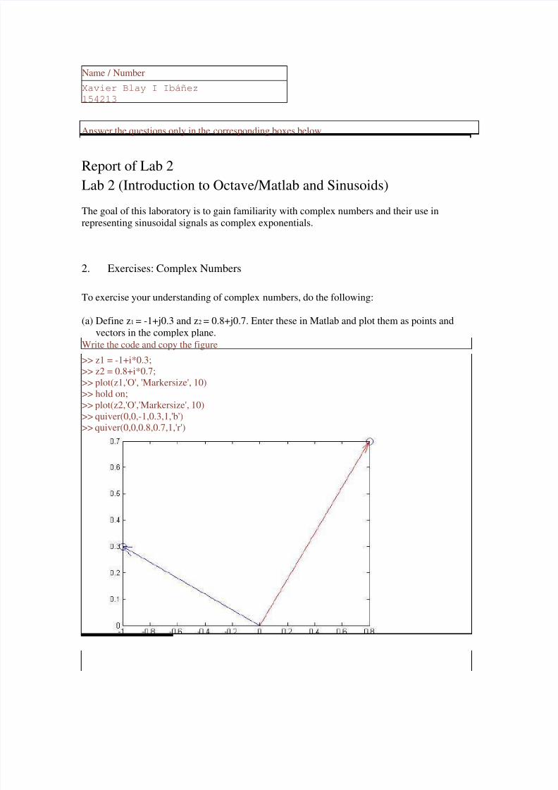
(a) Define z1 = -1+j0.3 and z2 = 0.8+j0.7. Enter these in Matlab and plot them as points and

vectors in the complex plane.

Write the code and copy the figure

>> z1 = -1+i*0.3;>> z2 = 0.8+i*0.7;

>> plot(z1,'O', 'Markersize', 10)>> hold on;

>> plot(z2,'O','Markersize', 10)

>> quiver(0,0,-1,0.3,1,'b')>> quiver(0,0,0.8,0.7,1,'r')

7/27/2019 Report for Lab 2 154213


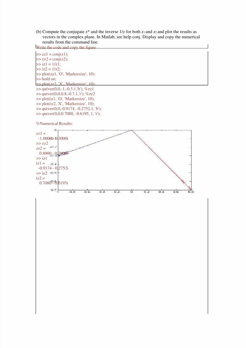
(b) Compute the conjugate z* and the inverse 1/z for both z1 and z2 and plot the results as

vectors in the complex plane. In Matlab, see help conj. Display and copy the numerical

results from the command line.


>> zz1 = conj(z1);

>> zz2 = conj(z2);>> iz1 = 1/z1;>> iz2 = 1/z2;

>> plot(zz1, 'O', 'Markersize', 10);>> hold on;

>> plot(zz2, 'X', 'Markersize', 10);

>> quiver(0,0,-1,-0.3,1,'b'); %zz1>> quiver(0,0,0.8,-0.7,1,'r'); %zz2

>> plot(iz1, 'O', 'Markersize', 10);>> plot(iz2, 'X', 'Markersize', 10);>> quiver(0,0,-0.9174, -0.2752,1, 'b');

>> quiver(0,0,0.7080, -0.6195, 1, 'r');

%Numerical Results:

zz1 =

-1.0000 - 0.3000i>> zz2

zz2 =

0.8000 - 0.7000i>> iz1

iz1 =-0.9174 - 0.2752i

>> iz2

iz2 =

0.7080 - 0.6195i

7/27/2019 Report for Lab 2 154213


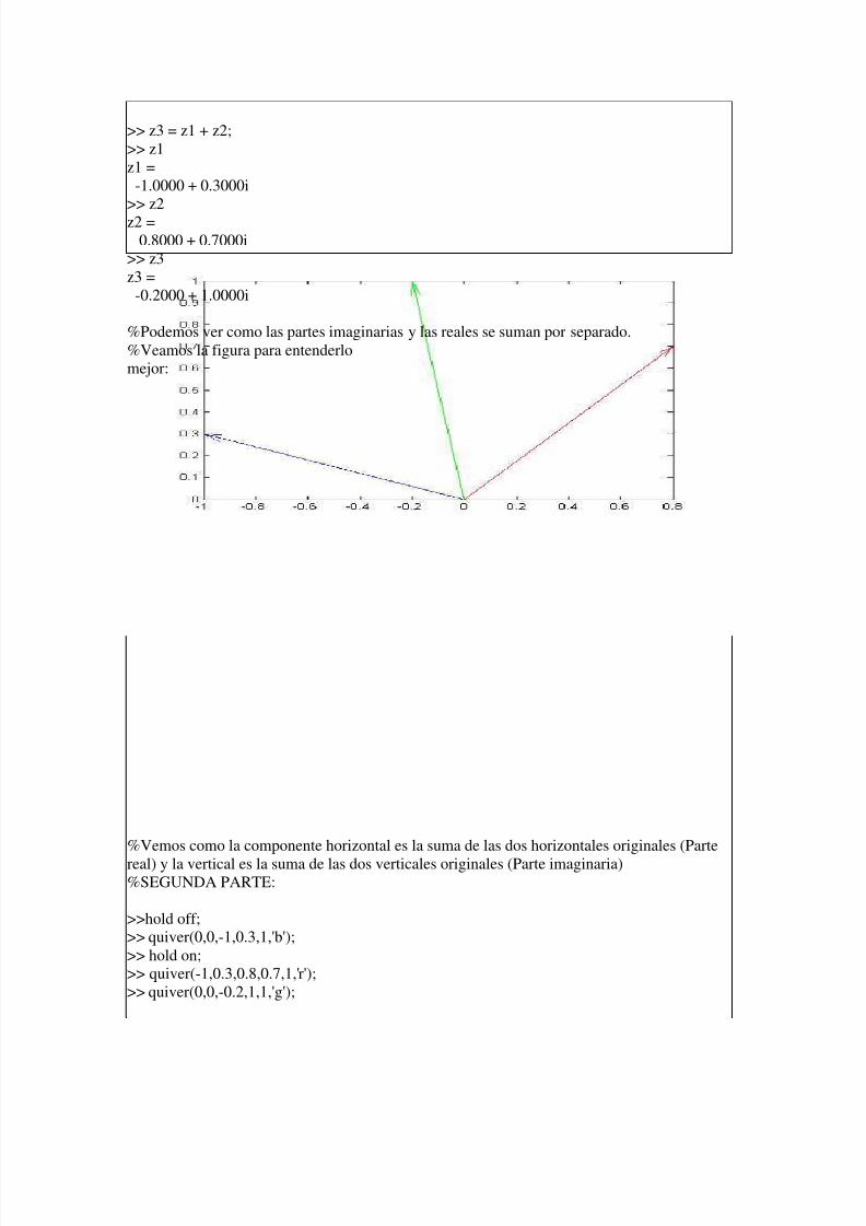
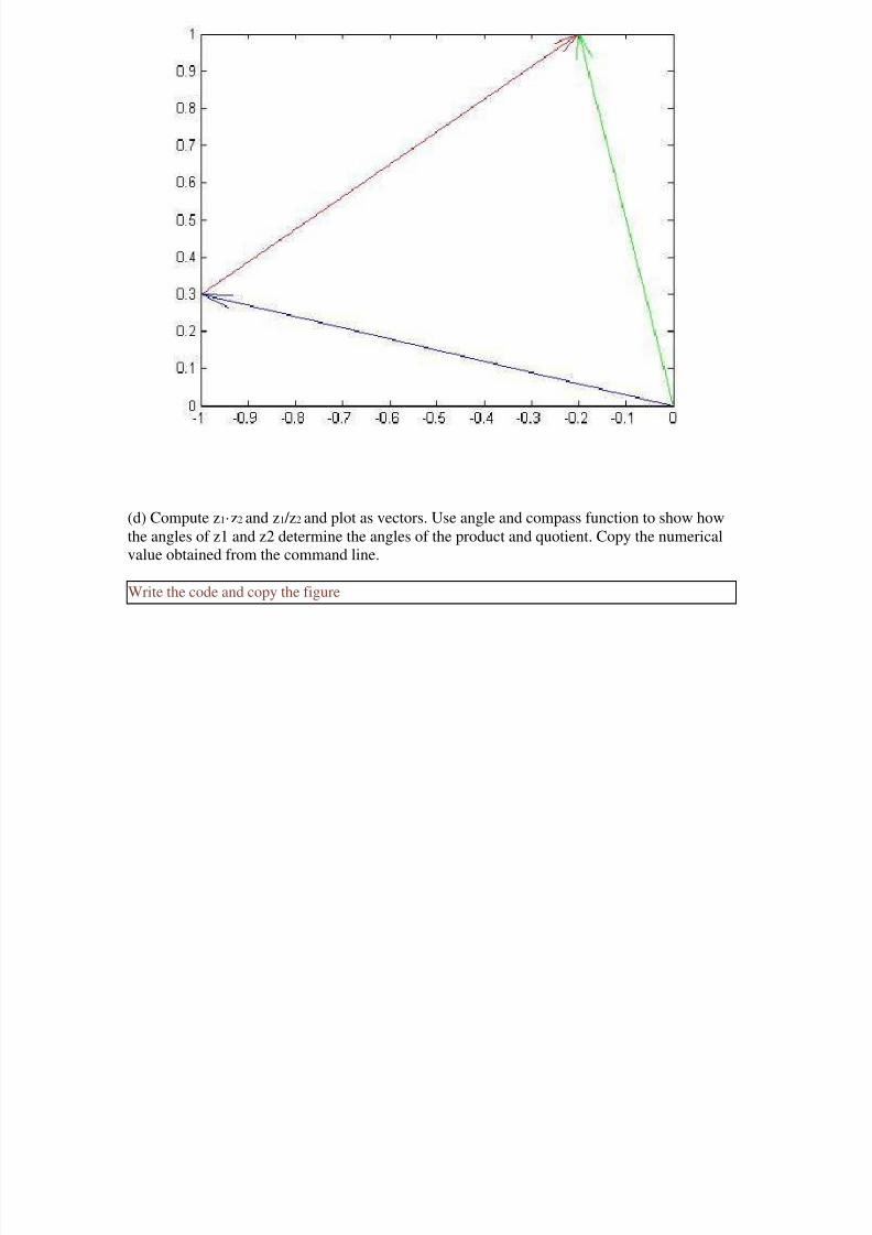
(c) Compute z1 +z2. Copy the result and display z1, z2, and z1+z2 as vectors in the complex plane.

Explain this result geometrically. Display again the previous complex numbers, but now plot

z1 and z1+z2 as vectors starting at the origin but z2 starting at the end of z1. Does this new plotagree with your geometrical interpretation?

Write the code and copy the figure, explain the result

7/27/2019 Report for Lab 2 154213


>> z3 = z1 + z2;

>> z1

z1 =

-1.0000 + 0.3000i

>> z2

z2 =

0.8000 + 0.7000i

>> z3

z3 =

-0.2000 + 1.0000i

%Podemos ver como las partes imaginarias y las reales se suman por separado.

%Veamos la figura para entenderlo

mejor:

%Vemos como la componente horizontal es la suma de las dos horizontales originales (Parte

real) y la vertical es la suma de las dos verticales originales (Parte imaginaria)%SEGUNDA PARTE:

>>hold off;

>> quiver(0,0,-1,0.3,1,'b');

>> hold on;

>> quiver(-1,0.3,0.8,0.7,1,'r');

>> quiver(0,0,-0.2,1,1,'g');

7/27/2019 Report for Lab 2 154213


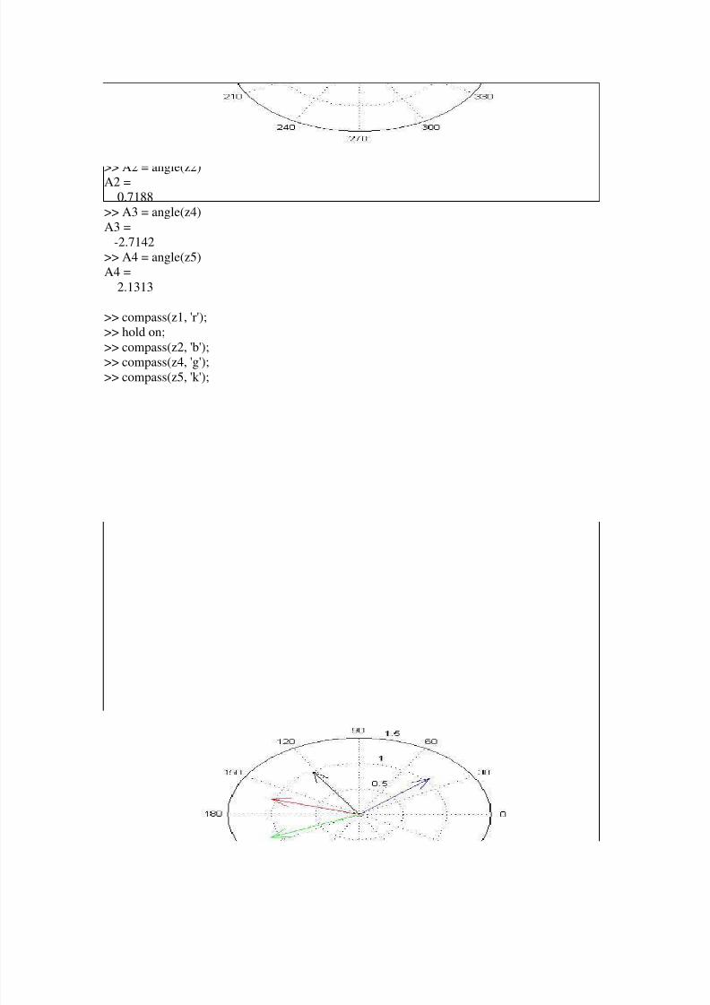
(d) Compute z1·z2 and z1 /z2 and plot as vectors. Use angle and compass function to show how

the angles of z1 and z2 determine the angles of the product and quotient. Copy the numerical

value obtained from the command line.


7/27/2019 Report for Lab 2 154213


>> z4 = z1 * z2;

>> z5 = z1 / z2;

>> A1 = angle(z1)

A1 =

2.8501

>> A2 = angle(z2)

A2 =

0.7188

>> A3 = angle(z4)

A3 =

-2.7142

>> A4 = angle(z5)

A4 =

2.1313

>> compass(z1, 'r');

>> hold on;

>> compass(z2, 'b');>> compass(z4, 'g');

>> compass(z5, 'k');

7/27/2019 Report for Lab 2 154213


3. Exercises: Complex Exponentials

3.1 Representation of Sinusoids with Complex Exponentials

In Matlab consult help on exp, real and imag.

(a) Generate the signal x(t)=

A

e j(ω0

t+

φ) for A=

3, φ=−

0.4π, andω0=

2π

1250. Takea range for t that will cover 2 or 3 periods.

Write the code

>> A=3; phi = -0.4*pi; wo = 2*pi*1250;

>> To = 1/1250;

>> tt = (-To:(To/100):4*To);

>> xx = A * exp(i*(wo*tt+phi));

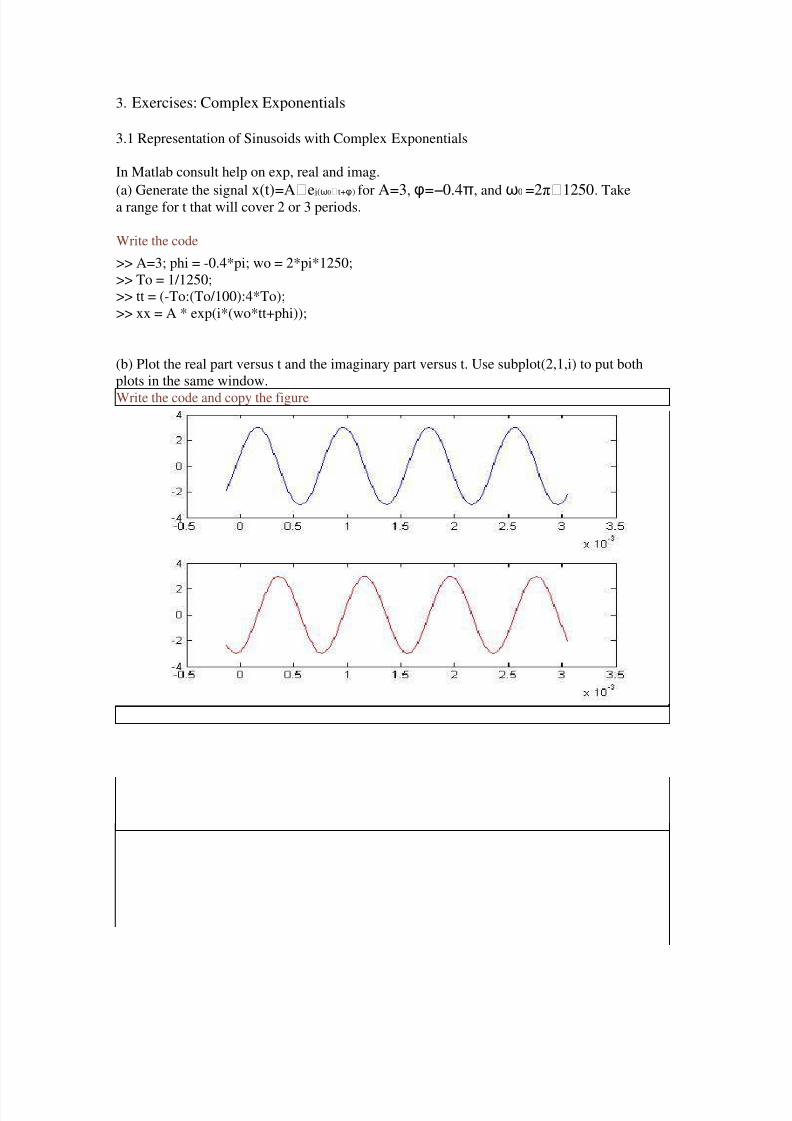
(b) Plot the real part versus t and the imaginary part versus t. Use subplot(2,1,i) to put both

plots in the same window.


>> xx = A * exp(i*(wo*tt+phi));

>> Re = real(xx);

>> subplot(2, 1, 1);

>> plot(tt, Re);

>> Im = imag(xx);

>> subplot(2, 1, 2);

>> plot(tt, Im, ‘r’);

7/27/2019 Report for Lab 2 154213


(c) Verify that the real and imaginary parts are sinusoids and that they have the correct

frequency, phase and amplitude.


Podemos ver en la anterior figura que efectivamente se trata de dos sinusoides.

Tanto la amplitud, como la frecuencia se puede ver a simple vista que se trata de la mismapara los dos elementos.

Vemos finalmente como la fase imaginaria está adelantada respecto la Real.

3.2 Verify Addition of Sinusoids Using Complex Exponentials

Generate four sinusoids with the following amplitudes and phases:

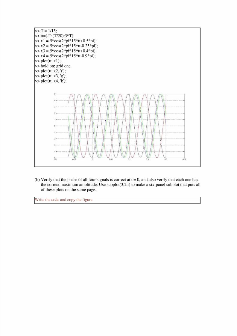
(a) Make a plot of all four signals over a range of t that will exhibit approximately 3 cycles.

Make sure the plot includes negative time so that the phase at t = 0 can be measured. In

order to get a smooth plot make sure that your have at least 20 samples per period of the

wave.


7/27/2019 Report for Lab 2 154213


>> T = 1/15;

>> tt=[-T:(T/20):3*T];

>> x1 = 5*cos(2*pi*15*tt+0.5*pi);

>> x2 = 5*cos(2*pi*15*tt-0.25*pi);

>> x3 = 5*cos(2*pi*15*tt+0.4*pi);

>> x4 = 5*cos(2*pi*15*tt-0.9*pi);

>> plot(tt, x1);

>> hold on; grid on;

>> plot(tt, x2, 'r');

>> plot(tt, x3, 'g');

>> plot(tt, x4, 'k');

(b) Verify that the phase of all four signals is correct at t = 0, and also verify that each one has

the correct maximum amplitude. Use subplot(3,2,i) to make a six-panel subplot that puts all

of these plots on the same page.


7/27/2019 Report for Lab 2 154213


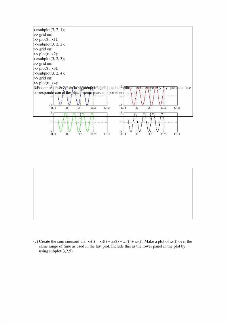
>>subplot(3, 2, 1);

>> grid on;

>> plot(tt, x1);

>>subplot(3, 2, 2);

>> grid on;

>> plot(tt, x2);

>>subplot(3, 2, 3);

>> grid on;

>> plot(tt, x3);

>>subplot(3, 2, 4);

>> grid on;

>> plot(tt, x4);

%Podemos observar en la siguiente imagen que la amplitud oscila entre -5 y 5 y que cada fase

corresponde con el desplazamiento marcado por el enunciado.

(c) Create the sum sinusoid via: x5(t) = x1(t) + x2(t) + x3(t) + x4(t). Make a plot of x5(t) over the

same range of time as used in the last plot. Include this as the lower panel in the plot by

using subplot(3,2,5).

7/27/2019 Report for Lab 2 154213



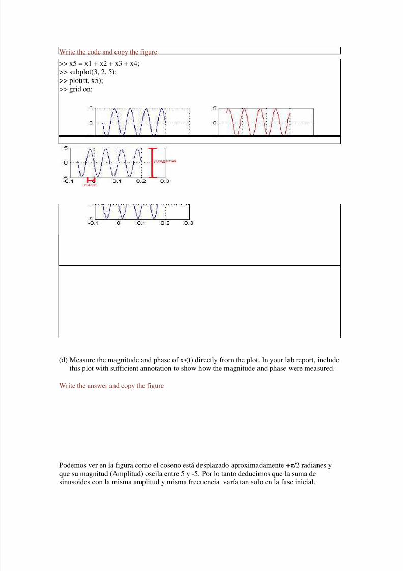
>> x5 = x1 + x2 + x3 + x4;

>> subplot(3, 2, 5);

>> plot(tt, x5);

>> grid on;

(d) Measure the magnitude and phase of x5(t) directly from the plot. In your lab report, include

this plot with sufficient annotation to show how the magnitude and phase were measured.

Write the answer and copy the figure

Podemos ver en la figura como el coseno está desplazado aproximadamente +π /2 radianes y

que su magnitud (Amplitud) oscila entre 5 y -5. Por lo tanto deducimos que la suma de

sinusoides con la misma amplitud y misma frecuencia varía tan solo en la fase inicial.

7/27/2019 Report for Lab 2 154213


(e) Now do some complex arithmetic; create the complex amplitudes corresponding to the

sinusoids xi(t):

Give the numerical values of zi in polar and Cartesian form.

Write the code and results

%Forma Polar:

>> z1 = 5 * exp(i*0.5*pi);

>> z2 = 5 * exp(i*-0.25*pi);

>> z3 = 5 * exp(i*0.4*pi);

>> z4 = 5 * exp(i*-0.9*pi);

>> z5 = 5 * exp(i*+0.5*pi);

%Forma Cartesiana:

>> z1

z1 = 0.0000 + 5.0000i>> z2

z2 = 3.5355 - 3.5355i

>> z3

z3 = 1.5451 + 4.7553i

>> z4

z4 = -4.7553 - 1.5451i

>> z5

z5 = 0.0000 - 5.0000i

(f) Verify that z5 = z1 +z2 +z3 +z4. Show a plot of these five complex numbers as vectors.


7/27/2019 Report for Lab 2 154213


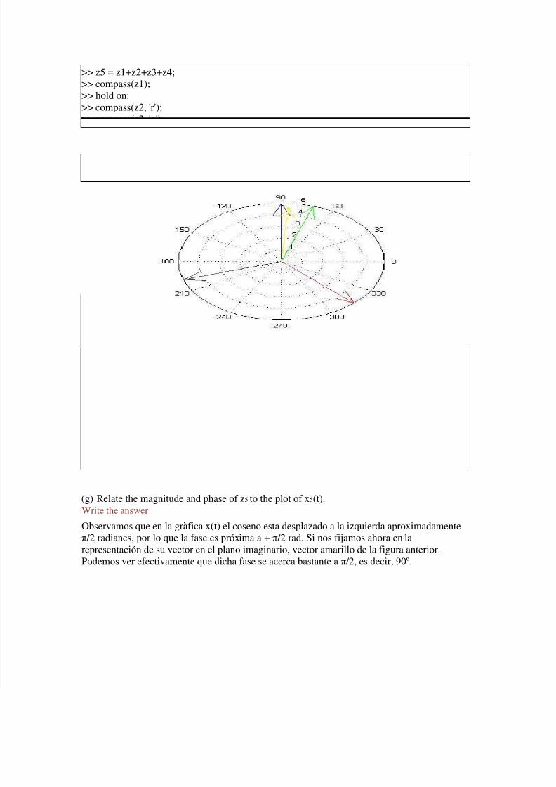
>> z5 = z1+z2+z3+z4;

>> compass(z1);

>> hold on;

>> compass(z2, 'r');

>> compass(z3, 'g');

>> compass(z4, 'k');

>> compass(z5, 'y');

(g) Relate the magnitude and phase of z5 to the plot of x5(t).

Write the answer

Observamos que en la gràfica x(t) el coseno esta desplazado a la izquierda aproximadamente

π /2 radianes, por lo que la fase es próxima a + π /2 rad. Si nos fijamos ahora en la

representación de su vector en el plano imaginario, vector amarillo de la figura anterior.Podemos ver efectivamente que dicha fase se acerca bastante a π /2, es decir, 90º.

Documents

Report for Lab 2 154213