TABLE OF CONTENT

Number Description Page

Student Ethic Code

Group Members 2

1.0 Objective of the experiment 3

2.0 Learning Outcomes 3

3.0 Introduction 3

4.0 Theory 3

5.0 Apparatus 6

6.0 Procedures 7

7.0 Result 8

8.0 Calculation 10

9.0 Discussion 20

10.0 Conclusion 22

11.0 References 23

Appendix 24

From left : Utaya, Zulkifli, Firdaus and Hafiz Anuar

1.0 OBJECTIVE

1.1 Part 1 : To plot moment influence line

1.2 Part 2 : To apply the use of a moment influence on a simply supported

beam

2.0 LEARNING OUTCOMES

2.1 Application of engineering knowledge in practical application

2.2 To enhance the technical competency in civil engineering through

laboratory application.

2.3 Communicate effectively in group.

2.4 To identify problem, solving and finding out appropriate solution through

laboratory application.

3.0 INTRODUCTION

Moving loads on beam are common features of design. Many road bridges are

constructed from beam, and as such have to be designed to carry a knife edge load,

or a string of wheel loads, or a uniformly distributed load, or perhaps the worst

combination of all three. To find the critical moment in section, influence line is

used.

4.0 THEORY

Definition: Influence line is defined as a line representing the changes in moment,

shear force, reaction or displacement at a section of a beam when a unit load moves

on the beam.

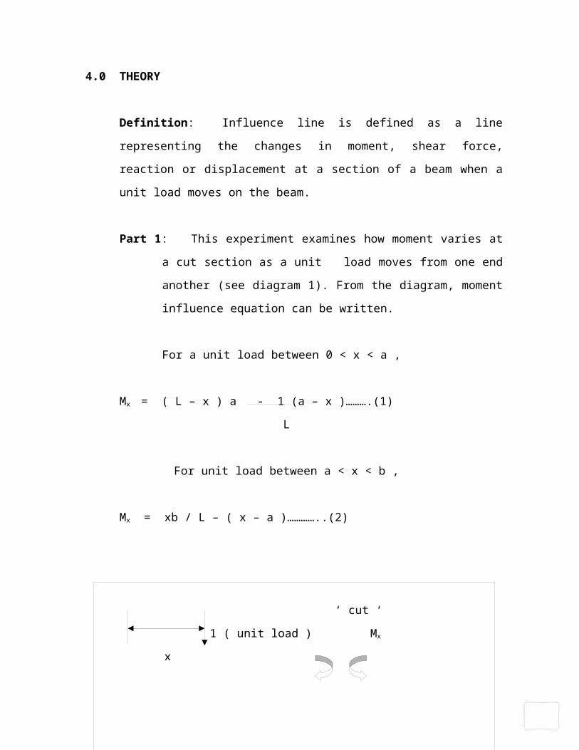
Part 1: This experiment examines how moment varies at a cut section as a unit

load moves from one end another (see diagram 1). From the diagram,

moment influence equation can be written.

For a unit load between 0 < x < a ,

Mx = ( L – x ) a - 1 (a – x )……….(1)

L

For unit load between a < x < b ,

Mx = xb / L – ( x – a )…………..(2)

‘ cut ‘

1 ( unit load ) Mx

x

Mx

RA = (1-x/L) RB = x/L

a b

L

Figure 1

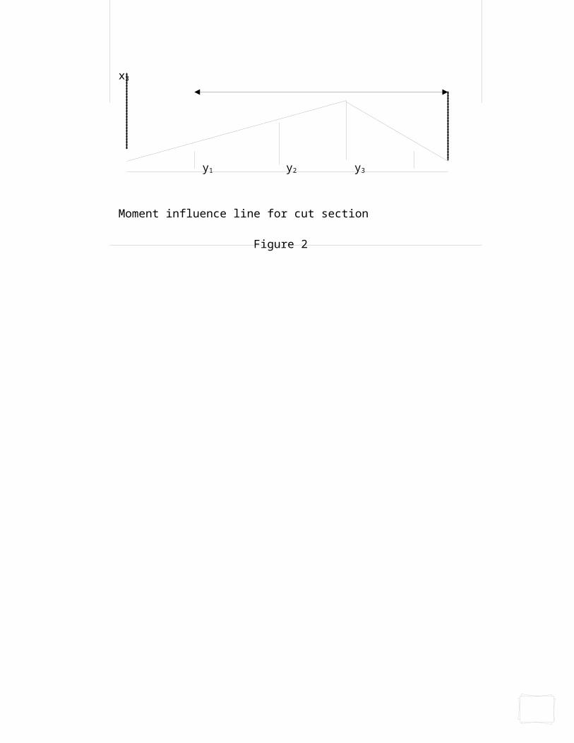
Part 2: If the beam is loaded as shown below, the moment at the ‘cut’ can be

calculated using the influence line. (See diagram 2).

Moment at the ‘cut’ section = F1y1 + F2y2 + F3y3 ……….(3)

( y1, y2, and y3 are coordinates derived from the influence line in terms of x1, x2, x3, a,

b and L )

a+b = L

x1

x2

x3

y1 y2 y3

Moment influence line for cut section

Figure 2

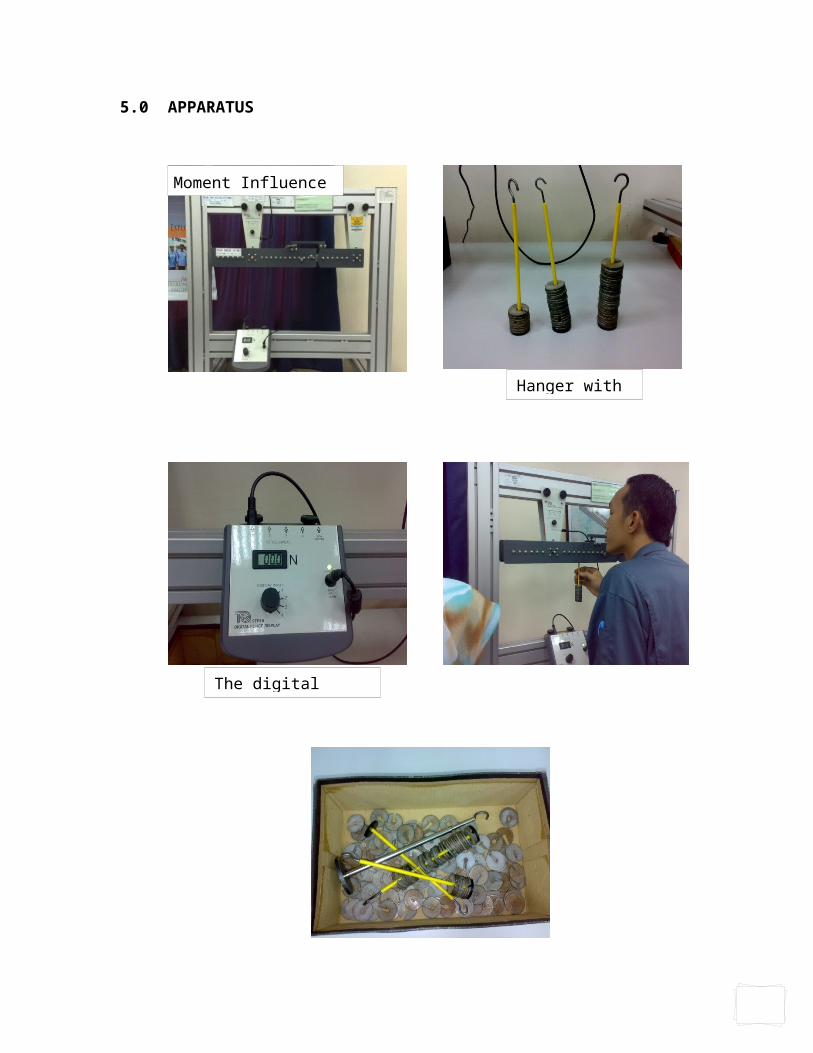
5.0 APPARATUS

Moment Influence Line

Hanger with load

The digital forces meter

6.0 PROCEDURES

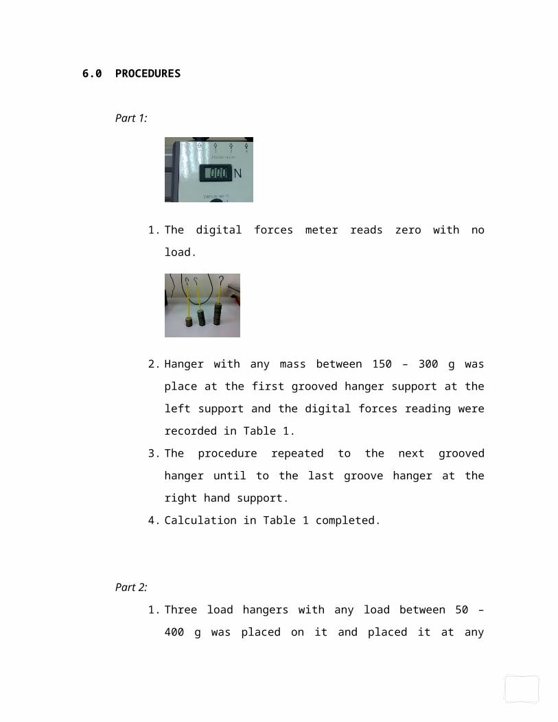
Part 1:

1. The digital forces meter reads zero with no load.

2. Hanger with any mass between 150 – 300 g was place at the first

grooved hanger support at the left support and the digital forces reading

were recorded in Table 1.

3. The procedure repeated to the next grooved hanger until to the last

groove hanger at the right hand support.

4. Calculation in Table 1 completed.

Part 2:

1. Three load hangers with any load between 50 – 400 g was placed on it

and placed it at any position between the supports. The position and the

digital forces display reading recorded in Table 2.

2. The procedure repeated with three other location.

3. The calculation in Table 2 completed.

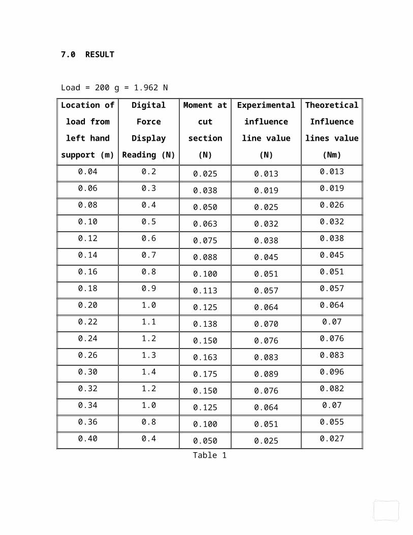
7.0 RESULT

Load = 200 g = 1.962 N

Location of

load from left

hand support

(m)

Digital Force

Display

Reading (N)

Moment at

cut section

(N)

Experimental

influence line

value (N)

Theoretical

Influence lines

value (Nm)

0.04 0.2 0.025 0.013 0.013

0.06 0.3 0.038 0.019 0.019

0.08 0.4 0.050 0.025 0.026

0.10 0.5 0.063 0.032 0.032

0.12 0.6 0.075 0.038 0.038

0.14 0.7 0.088 0.045 0.045

0.16 0.8 0.100 0.051 0.051

0.18 0.9 0.113 0.057 0.057

0.20 1.0 0.125 0.064 0.064

0.22 1.1 0.138 0.070 0.07

0.24 1.2 0.150 0.076 0.076

0.26 1.3 0.163 0.083 0.083

0.30 1.4 0.175 0.089 0.096

0.32 1.2 0.150 0.076 0.082

0.34 1.0 0.125 0.064 0.07

0.36 0.8 0.100 0.051 0.055

0.40 0.4 0.050 0.025 0.027

Table 1

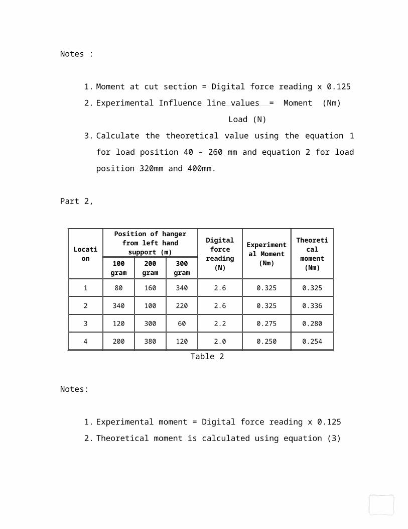
Notes :

1. Moment at cut section = Digital force reading x 0.125

2. Experimental Influence line values = Moment (Nm)

Load (N)

3. Calculate the theoretical value using the equation 1 for load position 40 – 260

mm and equation 2 for load position 320mm and 400mm.

Part 2,

Location

Position of hanger from left hand support (m) Digital

force reading (N)

Experimental Moment

(Nm)

Theoretical moment

(Nm)100 gram

200 gram

300 gram

1 80 160 340 2.6 0.325 0.325

2 340 100 220 2.6 0.325 0.336

3 120 300 60 2.2 0.275 0.280

4 200 380 120 2.0 0.250 0.254

Table 2

Notes:

1. Experimental moment = Digital force reading x 0.125

2. Theoretical moment is calculated using equation (3)

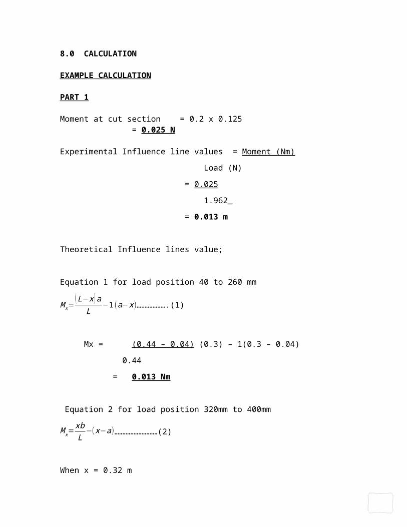
8.0 CALCULATION

EXAMPLE CALCULATION

PART 1

Moment at cut section= 0.2 x 0.125= 0.025 N

Experimental Influence line values = Moment (Nm)

Load (N)

= 0.025

1.962

= 0.013 m

Theoretical Influence lines value;

Equation 1 for load position 40 to 260 mm

M x=( L−x ) a

L−1(a−x )……………….(1)

Mx = (0.44 – 0.04) (0.3) – 1(0.3 – 0.04)

0.44

= 0.013 Nm

Equation 2 for load position 320mm to 400mm

M x=xbL

−(x−a)………………………(2)

When x = 0.32 m

Mx = (0.32) (0.14) – (0.32 – 0.3)

0.44

= 0.082 Nm

y1

y3

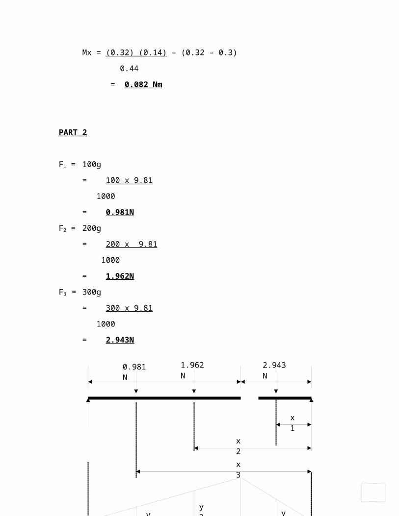
0.981 N 1.962 N 2.943 N

x1

x2

x3

y2

PART 2

F1 = 100g

= 100 x 9.81

1000

= 0.981N

F2 = 200g

= 200 x 9.81

1000

= 1.962N

F3 = 300g

= 300 x 9.81

1000

= 2.943N

Moment influence line for cut section

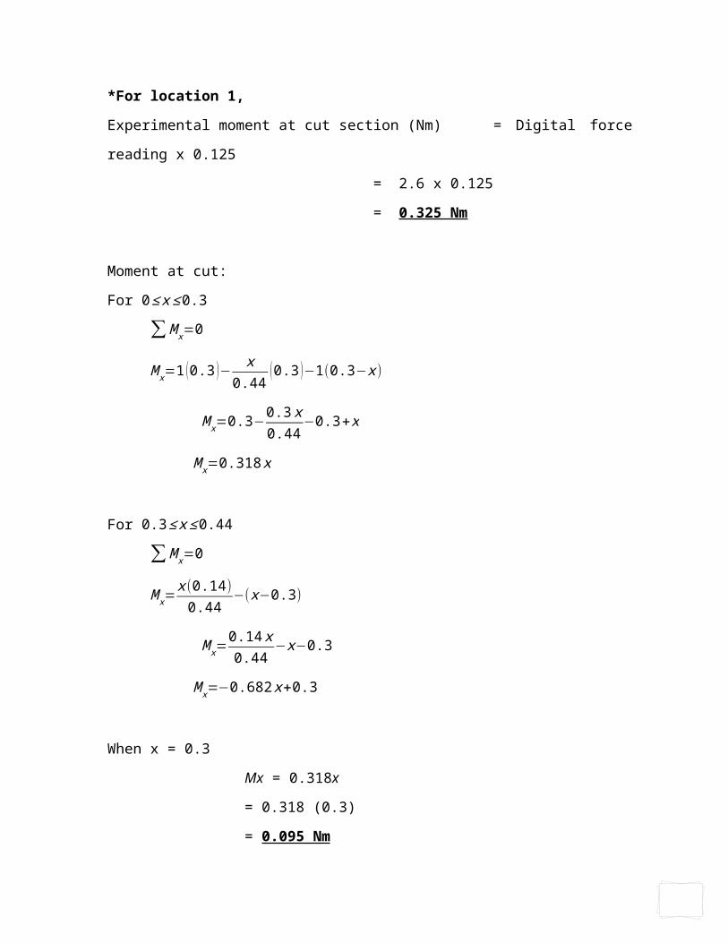
*For location 1,

Experimental moment at cut section (Nm) = Digital force reading x 0.125

= 2.6 x 0.125

= 0.325 Nm

Moment at cut:

For 0 ≤ x≤ 0.3

∑ M x=0

M x=1 (0.3 )− x0.44

(0.3 )−1(0.3−x)

M x=0.3−0.3 x0.44

−0.3+x

M x=0.318x

For 0.3 ≤ x≤ 0.44

∑ M x=0

M x=x (0.14)

0.44−(x−0.3)

M x=0.14 x0.44

−x−0.3

M x=−0.682 x+0.3

When x = 0.3

Mx = 0.318x

= 0.318 (0.3)

= 0.095 Nm

M x=−0.682 x+0.3

= - 0.682 (0.3) + 0.3

= - 0.095 Nm

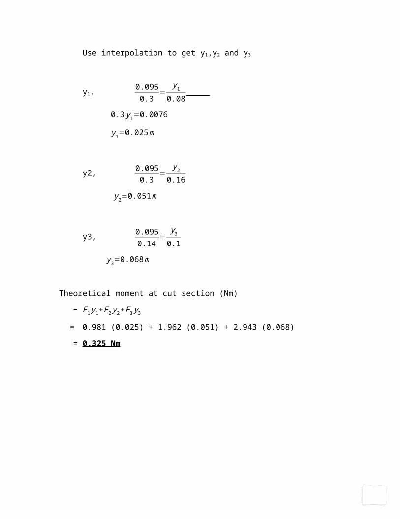
Use interpolation to get y1,y2 and y3

y1, 0.0950.3

=y1

0.08

0.3 y1=0.0076

y1=0.025 m

y2, 0.0950.3

=y2

0.16

y2=0.051 m

y3, 0.0950.14

=y3

0.1

y3=0.068 m

Theoretical moment at cut section (Nm)

= F1 y1+F2 y2+F3 y3

= 0.981 (0.025) + 1.962 (0.051) + 2.943 (0.068)

= 0.325 Nm

y1

y3

1.962 N 2.943 N 0.981 N

x1

x2

x3

y2

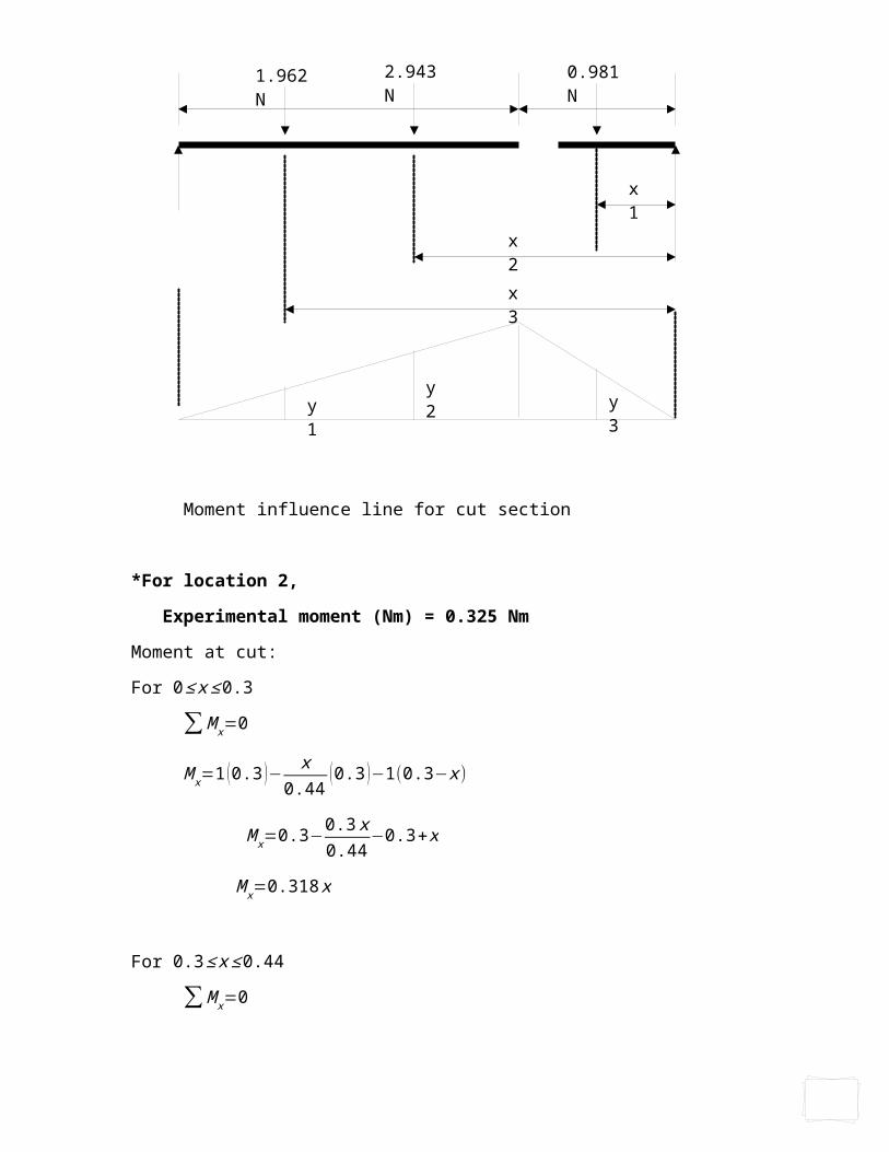
Moment influence line for cut section

*For location 2,

Experimental moment (Nm) = 0.325 Nm

Moment at cut:

For 0 ≤ x≤ 0.3

∑ M x=0

M x=1 (0.3 )− x0.44

(0.3 )−1(0.3−x)

M x=0.3−0.3 x0.44

−0.3+x

M x=0.318x

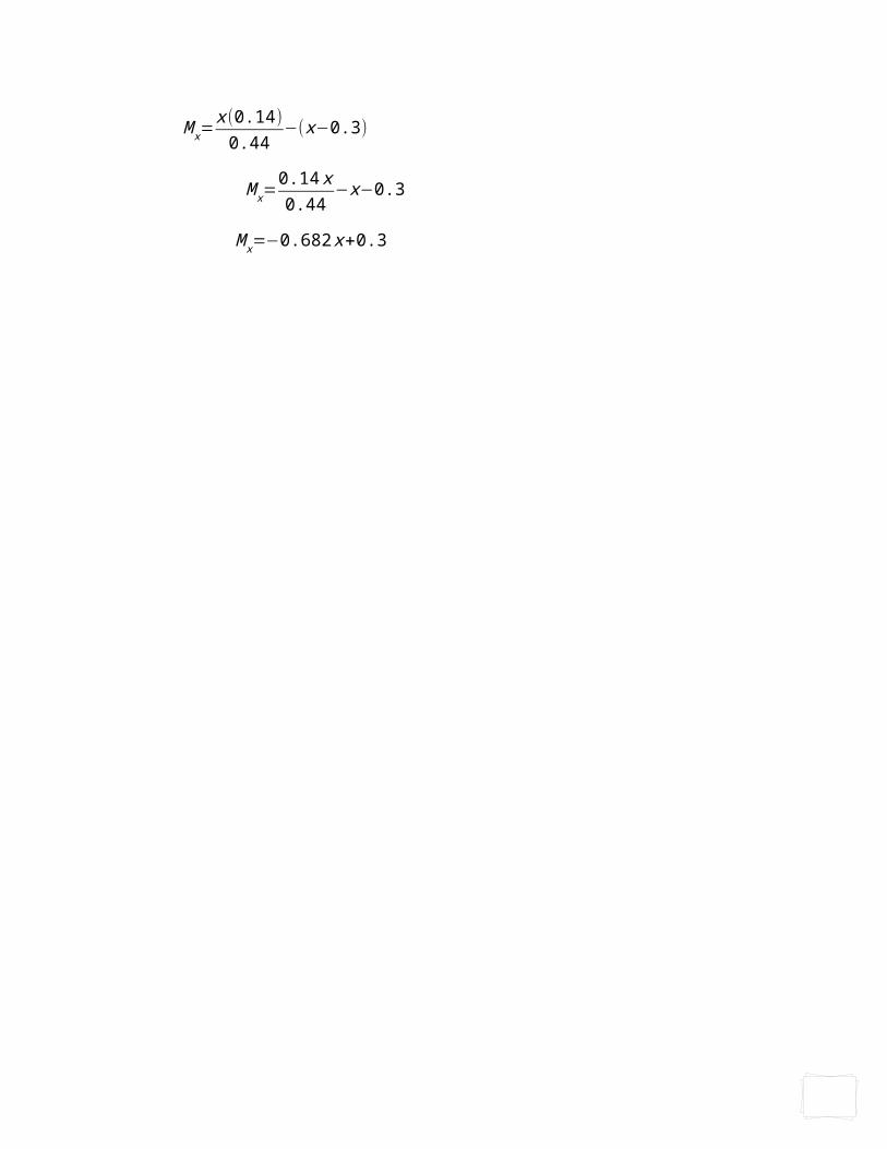
For 0.3 ≤ x≤ 0.44

∑ M x=0

M x=x (0.14)

0.44−(x−0.3)

M x=0.14 x0.44

−x−0.3

M x=−0.682 x+0.3

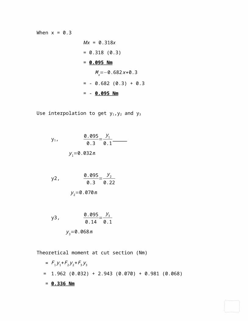
When x = 0.3

Mx = 0.318x

= 0.318 (0.3)

= 0.095 Nm

M x=−0.682 x+0.3

= - 0.682 (0.3) + 0.3

= - 0.095 Nm

Use interpolation to get y1,y2 and y3

y1, 0.0950.3

=y1

0.1

y1=0.032 m

y2, 0.0950.3

=y2

0.22

y2=0.070m

y3, 0.0950.14

=y3

0.1

y3=0.068 m

Theoretical moment at cut section (Nm)

= F1 y1+F2 y2+F3 y3

= 1.962 (0.032) + 2.943 (0.070) + 0.981 (0.068)

= 0.336 Nm

y1

y3

2.941 N 0.981 N 1.962 N

x1

x2

x3

y2

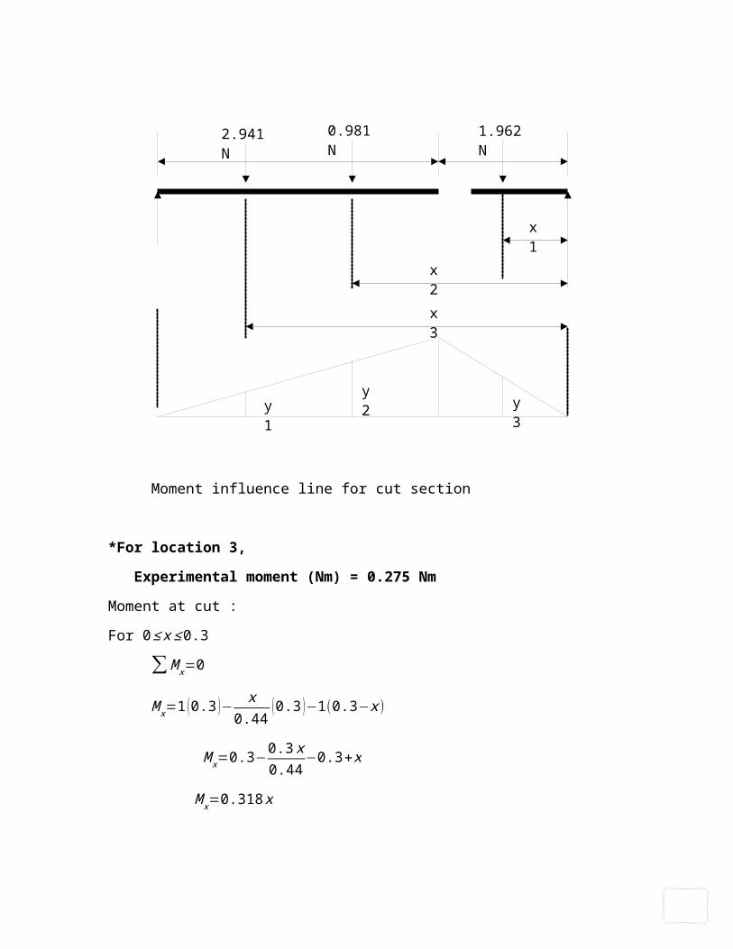
Moment influence line for cut section

*For location 3,

Experimental moment (Nm) = 0.275 Nm

Moment at cut :

For 0 ≤ x≤ 0.3

∑ M x=0

M x=1 (0.3 )− x0.44

(0.3 )−1(0.3−x)

M x=0.3−0.3 x0.44

−0.3+x

M x=0.318x

For 0.3 ≤ x≤ 0.44

∑ M x=0

M x=x (0.14)

0.44−(x−0.3)

M x=0.14 x0.44

−x−0.3

M x=−0.682 x+0.3

When x = 0.3

Mx = 0.318x

= 0.318 (0.3)

= 0.095 Nm

M x=−0.682 x+0.3

= - 0.682 (0.3) + 0.3

= - 0.095 Nm

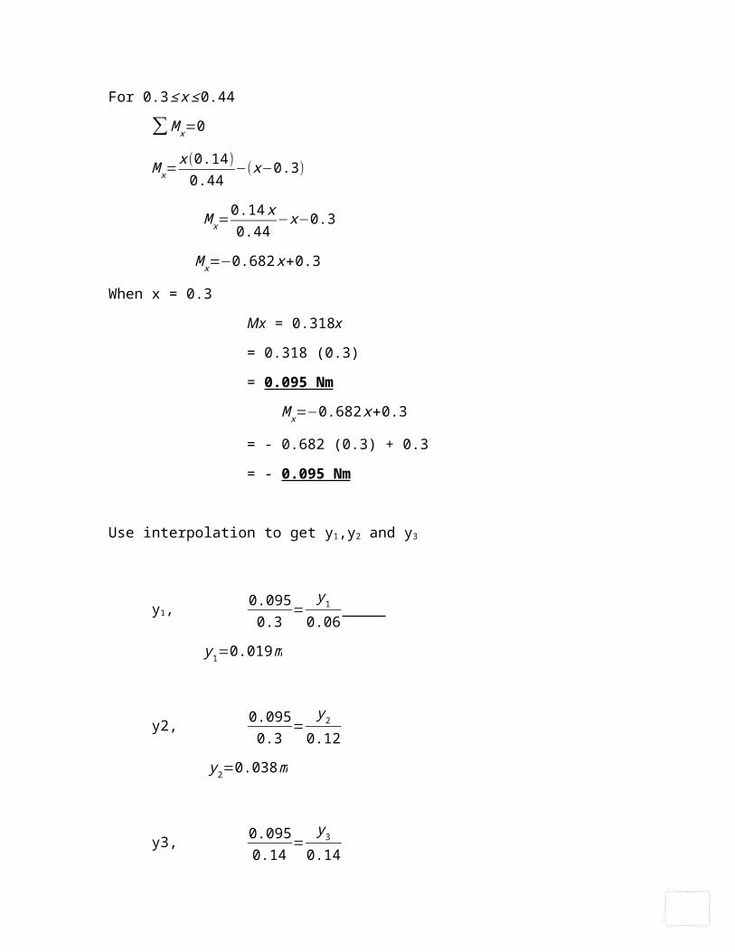
Use interpolation to get y1,y2 and y3

y1, 0.0950.3

=y1

0.06

y1=0.019 m

y2, 0.0950.3

=y2

0.12

y2=0.038m

y3, 0.0950.14

=y3

0.14

y3=0.095 m

Theoretical moment at cut section (Nm)

= F1 y1+F2 y2+F3 y3

= 2.943 (0.019) + 0.981 (0.038) + 1.962 (0.095)

= 0.280 Nm

y1

y3

2.941 N 0.981 N 1.962 N

x1

x2

x3

y2

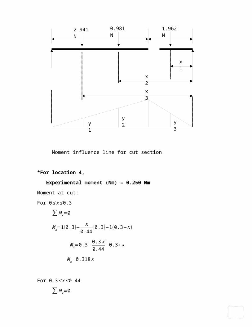
Moment influence line for cut section

*For location 4,

Experimental moment (Nm) = 0.250 Nm

Moment at cut:

For 0 ≤ x≤ 0.3

∑ M x=0

M x=1 (0.3 )− x0.44

(0.3 )−1(0.3−x)

M x=0.3−0.3 x0.44

−0.3+x

M x=0.318x

For 0.3 ≤ x≤ 0.44

∑ M x=0

M x=x (0.14)

0.44−(x−0.3)

M x=0.14 x0.44

−x−0.3

M x=−0.682 x+0.3

When x = 0.3

Mx = 0.318x

= 0.318 (0.3)

= 0.095 Nm

M x=−0.682 x+0.3

= - 0.682 (0.3) + 0.3

= - 0.095 Nm

Use interpolation to get y1,y2 and y3

y1, 0.0950.3

=y1

0.12

y1=0.038 m

y2, 0.0950.3

=y2

0.2

y2=0.063m

y3, 0.0950.14

=y3

0.06

y3=0.041m

Theoritical moment at cut section (Nm)

= F1 y1+F2 y2+F3 y3

= 2.943 (0.038) + 0.981 (0.063) + 1.962 (0.041)

= 0.254 Nm

F1

a b

cut

RA = = RB

x

L

9.0 DISCUSSIONS

PART 1

1. Derive equation 1 and 2.

∑ F x=0

∑ F y=R A+RB−1=0

RA+RB=1

∑ M x=0

RA ( L )−1 ( L−x )=0

RA L=1 (L−x)

RA=1(L−x)

L

¿1−x

L

RA+RB=1

RB=1−(1−x)

L

RB=xL

Equation 1 ; 0 ≤ x≤ a

−M x+RA (a)– 1(a−x )=0

M x=(1 – x)a

L– 1(a−x)

¿(L – x )a – 1(a−x)

L

Equation 2 ; a ≤ x≤ b

M x – RB(b)+1(x−a)=0

M x=RB(b)–1 (x−a)

¿ xL(b) – 1(x−a)

¿xbL

– 1(x−a)

2. On the graph, plot the theoretical and experimental value against distance from

left and support. Comment on the shape of graph. What does it tell u about how

moment varies at the cut section as a load moved on the beam?

0.040.08

0.120.16 0.2

0.24 0.30.34 0.4

00.020.040.060.08

0.10.120.140.160.18

0.2

Graph of Theoretical Value (Nm)versus Exper-imental Value (Nm) versus Distance (m)

Theoretical Influence lines value (Nm)Experimental influence line value (N)

Distance (m)

Mom

ent (

Nm

)

From the graph, a peak shaped graph can be obtained. The peak is the weakest point

of the beam where there is a hinge in the beam. As load is being moved on the

beam, the influence line which was constructed can be used to obtain the value of

the moment. As load is moved across near to it, the moment will increase. So does

the other way round when load is moving further than the hinge, the value of

moment will decrease as the load is moving towards the support at the end. As the

load is moving along towards the hinge from both side of support, it will come to a

peak where the value of moment is the same.

3. Comment on the experimental results and compare it to the theoretical results.

The experimental results that we obtained are quite accurate and compare to the

theoretical results, the experimental results are only slightly different with

theoretical results. When we were conducted the experiment, we tried to minimize

the error by ensuring the Digital Force Meter reads zero with no load before we

place the hangers.

PART 2

1. Calculate the percentage difference between experimental and theoretical results in

table 2. Comment on why the results differ.

Experimental Moment (Nm)

Theoretical moment (Nm)

Percentage Different (%)

0.325 0.325 00.325 0.336 3.270.275 0.280 1.790.250 0.254 1.57

The experimental results are slightly different from theoretical results are due to

human error and instrument sensitivity as the reading of the instrument keep

changing when we conducted the experiment.

10.0 CONCLUSION

As a conclusion, both objectives were achieved. Moment influence line could be

plot and the influence line can be use to determine the moment. We were able to

identify the reaction and behavior of a beam in terms of its moment reaction value.

This method is useful to check every cross section for a particular beam.

11.0 REFERENCES

Ando, J., Komatsuda, T., and Kamiya, A. 1988. Cytoplasmic calcium responses to fluid shear stress in cultured vascular endothelial cells. In Vitro 24: 871-877.

Ando, J., Nomura, H., and Kamiya, A. 1987. The effects of fluid shear stress on the migration and proliferation of cultured endothelial cells. Microvascular Research 33: 6270.

Caplan, B.A. and Schwartz, C.J. 1973. Increased endothelial cell turnover in areas of in vivo Evans blue uptake in the pig aorta. Atherosclerosis 17: 401-417.

Davies, P.F., Remuzzi, A., Gordon, EJ., Dewey, C.F., and Gimbrone, M.A. 1986. Turbulent fluid shear stress induces vascular endothelial cell turnover in vitro. Proceedings of the National Academy of Sciences U.S.A. 83: 2114-2117.

deSouza, P.A., Levesque, M.J., and Nerem, R.M. 1986. Electrophysiological response of endothelial cells to fluid- imposed shear stress. Federation Proceedings 45: 471.

Dewey, C.F., Jr., Bussolari, S.R., Gimbrone, M.A., Jr., and Davis, P.F. 1981. The dynamic response of vascular endothelial cells to fluid shear stress. Journal of Biomechanical Engineering 103: 177-185.

Diamond, S.L., Eskin, S.G., and McIntire, L.V. 1989. Fluid flow stimulates tissue plasminogen activator. Science 243: 1483-1485.

Frangos, J.A., McIntire, L.V., Eskin, S.G., and Ives, C.L. 1985. Flow effects on prostacyclin production by cultured human endothelial cells. Science 227: 1477-1479.

Leung, D.Y.M., Glagov, S., and Mathews, M.B. 1976. Cyclic stretching stimulates synthesis of matrix components by arterial smooth muscle cells in vitro. Science 191: 475-477.

Levesque, M.J., Liepsch, D., Moravec, S., and Nerem, R.M. 1986. Correlation of endothelial cell shape and wall shear stress in a stenosed dog aorta. Arteriosclerosis 6: 220229.

APPENDIX

Influence lines play an important part in the design of bridges, industrial crane

rails, conveyor belts, and other structures where loads move across their span.

An influence line represents the variation of the reaction, shear, moment, or deflection at a

specific point in a member as a concentrated force moves over the member. Once this line

is constructed, one can tell at a glance where the moving load should be placed on a

structure so that it creates the greatest influence at the specified point. Furthermore, the

magnitude of the associated reaction, shear, moment, or deflection at the point can than be

calculated from the ordinates of the influence line diagram.

A bending moment exists in a structural element when a moment is applied to the element

so that the element bends. Moments and torques are measured as a force multiplied by a

distance so they have as unit newton-metres (N·m) , or foot-pounds force (ft·lbf). The

concept of bending moment is very important in engineering (particularly

in civil and mechanical engineering) and physics.

Tensile stresses and compressive stresses increase proportionally with bending moment,

but are also dependent on the second moment of area of the cross-section of the structural

element. Failure in bending will occur when the bending moment is sufficient to induce

tensile stresses greater than the yield stress of the material throughout the entire cross-

section. It is possible that failure of a structural element in shear may occur before failure in

bending; however the mechanics of failure in shear and in bending are different.

The bending moment at a section through a structural element may be defined as "the sum

of the moments about that section of all external forces acting to one side of that section".

The forces and moments on either side of the section must be equal in order to counteract

each other and maintain a state of equilibrium so the same bending moment will result from

summing the moments, regardless of which side of the section is selected.

Moments are calculated by multiplying the external vector forces (loads or reactions) by

the vector distance at which they are applied. When analyzing an entire element, it is

sensible to calculate moments at both ends of the element, at the beginning, centre and end

of any uniformly distributed loads, and directly underneath any point loads. Of course any

"pin-joints" within a structure allow free rotation, and so zero moment occurs at these

points as there is no way of transmitting turning forces from one side to the other.

If clockwise bending moments are taken as negative, then a negative bending moment

within an element will cause "sagging", and a positive moment will cause "hogging". It is

therefore clear that a point of zero bending moment within a beam is a point of contra

flexure—that is the point of transition from hogging to sagging or vice versa.

It is more common to use the convention that a clockwise bending moment to the left of the

point under consideration is taken as positive. This then corresponds to the second

derivative of a function which, when positive, indicates a curvature that is 'lower at the

centre' i.e. sagging. When defining moments and curvatures in this way calculus can be

more readily used to find slopes and deflections.