Embed Size (px)
Citation preview

DEVELOPMENT OF EXPERIMENTAL INFLUENCE LINES
FOR BRIDGES
by
Jasmeen Hirachan
A thesis submitted to the Faculty of the University of Delaware in partial fulfillment of the requirements for the degree of Master of Civil Engineering.
Spring 2006
Copyright 2006 Jasmeen Hirachan All Rights Reserved

UMI Number: 1435843
14358432006
UMI MicroformCopyright
All rights reserved. This microform edition is protected against unauthorized copying under Title 17, United States Code.
ProQuest Information and Learning Company 300 North Zeeb Road
P.O. Box 1346 Ann Arbor, MI 48106-1346
by ProQuest Information and Learning Company.

DEVELOPMENT OF EXPERIMENTAL INFLUENCE LINES
FOR BRIDGES
by
Jasmeen Hirachan
Approved: __________________________________________________________ Michael J. Chajes, Ph.D. Professor in charge of thesis on behalf of the Advisory Committee Approved: __________________________________________________________ Michael J. Chajes, Ph.D. Chair of the Department of Civil and Environmental Engineering Approved: __________________________________________________________ Eric W. Kaler, Ph.D. Dean of the College of Engineering Approved: __________________________________________________________ Conrado M. Gempesaw II, Ph.D. Vice Provost for Academic and International Programs

ACKNOWLEDGMENTS
I am sincerely grateful to my advisor, Dr. Michael J. Chajes, for his
continuous guidance, advice and support. I also express my gratitude to the Delaware
Department of Transportation for providing funding for the bridge tests, with special
thanks to Mr. Doug Finney and Mr. Gerard Mulderig. I thank Mr. Steve Bisch of KCI,
the resident engineer for coordinating the testing schedule, and Mr. Jim Sullivan of
DelDOT for providing the load trucks. I also thank the design engineers, Mr. Richard
Martino and Mr. Anthony Temeles of Modjeski and Masters, for providing as-built
properties of the bridge. I am thankful also to the University of Delaware staff, and
students, Mr. Gary Wenczel, Ms. Melissa Williams and Mr. Michael Zettlemoyer,
who helped to conduct the test and to evaluate some of the data.
I express my heartfelt gratitude to my Dad, Mr. Manesh Hirachan, and
Mom, Mrs. Mangala Hirachan, and my sister, Ms. Kripa Hirachan, for all their love,
support and encouragement. Finally, I am deeply thankful to my husband, Mr. Sagar
Thakali, for his love and friendship always.
3

TABLE OF CONTENTS
LIST OF TABLES ............................................................................................. 5 LIST OF FIGURES............................................................................................ 6 ABSTRACT ....................................................................................................... 8
Chapter 1 ...................................................................................................................... 10 Introduction ...................................................................................................... 10
Chapter 2 ...................................................................................................................... 13 Background....................................................................................................... 13
Chapter 3 ...................................................................................................................... 16 Methodology..................................................................................................... 16
3.1 Influence lines ............................................................................. 16 3.2 Truck response ............................................................................ 16 3.3 Theoretical example .................................................................... 21
Chapter 4 ...................................................................................................................... 28 Eperimental approach....................................................................................... 28
4.1 Test case ...................................................................................... 28 4.2 Testing procedure ........................................................................ 36 4.3 Experimental example................................................................. 39
4.3.1 Passes 6 and 8:.............................................................. 39 4.3.2 Passes 7 and 10:............................................................ 50
Chapter 5 ...................................................................................................................... 58 Experimental influence line.............................................................................. 58
5.1 Test results................................................................................... 58 5.2 Influence lines for gage locations................................................ 62 5.3 Simple lever rule ......................................................................... 70 5.4 Application to load distribution................................................... 76 5.5 Sensitivity study .......................................................................... 81
Chapter 6 ...................................................................................................................... 87 Conclusion........................................................................................................ 87 Bibliography ..................................................................................................... 90
4
LIST OF TABLES
Table 4.1 Trucks used in the test ............................................................................. 35
Table 4.2 Truck passes ............................................................................................ 37
Table 4.3 Calculation of truck speed. ...................................................................... 41
5
LIST OF FIGURES
Figure 3.1 Truck response for long span bridge ...................................................... 18
Figure 3.2 Truck response for short span bridge ..................................................... 20
Figure 3.3 Theoretical example. a) Bridge geometry. b) Truck configuration........ 25
Figure 3.3 Theoretical example. c) Theoretical IL at B. d) Influence profile due to trucks. .......................................................................................... 26
Figure 3.3 Theoretical example. e) IL derived after subtraction of IP’s. f) Final IL after offsetting distance. ........................................................... 27
Figure 4.1 South market street bridge...................................................................... 29
Figure 4.2 South leaf framing plan of the bridge..................................................... 32
Figure 4.3 Strain gages clamped at the floor beam ................................................. 34
Figure 4.4 Truck passing over the bridge ................................................................ 38
Figure 4.5 Strain plots for pass 6 a) strain vs. time b) strain vs. distance. .............. 43
Figure 4.5 Strain plots for pass 6 c) strain vs. interpolated distance d) factored strain vs. distance. .................................................................... 44
Figure 4.6 Strain plots for pass 8. a) strain vs. time b) strain vs. distance. ............ 46
Figure 4.6 Strain plots for pass 8. c) strain vs. interpolated distance. .................... 47
Figure 4.7 Resulting strain plots. a) strain due to difference in front axle weight b) strain due to unit load............................................................. 49
Figure 4.8 Strain plots for pass 10. a) strain vs. time b) strain vs. distance. ........... 51
Figure 4.8 Strain plots for pass 10. c) factored strain vs. distance. ......................... 52
Figure 4.9 Strain plots for pass 7. a) strain vs. time b) strain vs. distance. ............. 54
6

Figure 4.10 Resulting strain plots. a) Strain due to difference in front axle weight. b) Strain due to unit load. .......................................................... 56
Figure 4.10 Resulting strain plots. c) Strain due to unit load. ................................... 57
Figure 5.1 Influence strains for passes a) 7 and 10 b) 5 and 9. ............................... 60
Figure 5.1 Influence strains for passes c) 6 and 8 d) 2and4. ................................... 61
Figure 5.2 Experimental strain influence lines for gages a) 303 b) 342.................. 63
Figure 5.2 Experimental strain influence lines for gages c) 318 d) 355.................. 64
Figure 5.2 Experimental strain influence lines for gages e) 346 f) 317. ................. 65
Figure 5.2 Experimental strain influence lines for gages g) 348 h) 338. ................ 66
Figure 5.3 Strain influence line for gage 355. ......................................................... 69
Figure 5.4 Example for simple lever rule. ............................................................... 70
Figure 5.5 Graphical representation of simple lever rule. ....................................... 73
Figure 5.6 Distance vs. strain influence line for three floor beams......................... 75
Figure 5.7 Comparison of strain influence lines obtained from passes 11 and 12 and final for gages a) 303 b) 342....................................................... 77
Figure 5.7 Comparison of strain influence lines obtained from passes 11 and 12 and final for gages c) 318 d) 355....................................................... 78
Figure 5.7 Comparison of strain influence lines obtained from passes 11 and 12 and final for gages e) 346 f) 317 ....................................................... 79
Figure 5.7 Comparison of strain influence lines obtained from passes 11 and 12 and final for gages g) 348 h) 338. ..................................................... 80
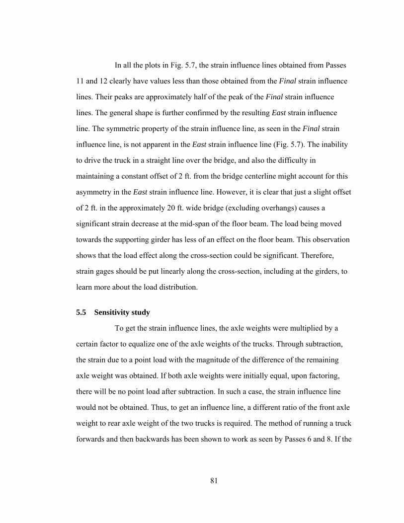
Figure 5.8 Strain vs. time plots for a) Pass 14 and b) Pass 6................................... 83
Figure 5.9 Magnified strain plots for a) Pass 14 and b) Pass 6. .............................. 84
Figure 5.10 Strain influence lines obtained from Pass 3 and Pass 14. ...................... 86
7

ABSTRACT
Ongoing deterioration of the nation’s bridge inventory, combined with
limited financial resources for maintaining it, makes the role of bridge management
more important than ever. In order to effectively manage a bridge inventory, bridge
owners need to know the condition of their bridges. It has been shown that calculation
of a bridge’s load carrying capacity using as-built details and standard design
equations most often under predicts the bridges actual capacity. While it is
understandable that design equations will yield conservative designs, when making
bridge management decisions, owners desire to have accurate condition assessments.
One effective method for evaluating a bridges current condition and load carrying
capacity is through the use of field load tests. An ideal field test would be conducted
with minimal instrumentation, minimal traffic interruption, and commonly available
load vehicles. In this thesis, a method for developing experimental influence lines
using field test data is developed. The influence lines produced are well suited for use
in quantifying how a particular bridge distributes loads, and can also be used to
estimate the load carrying capacity of the bridge. Test procedures for short to medium
span bridges, that utilize strain transducers and dump trucks and that are similar to
those used for diagnostic tests, are developed. Also developed is the methodology of
determining influence lines from the experimental data. Using the methodology
developed, the procedure is applied to the South Market Street bridge in Wilmington,
Delaware. Experimental influence lines that are developed for this bridge are used to
evaluate the load distribution to the floor beams of the bridge, and can be also be used
8

by the bridge owner to evaluate the safety of the bridge to carry multi-axle super
loads.
9

Chapter 1
INTRODUCTION
Over time, the number and weight of vehicles increases, and the
conditions of bridges deteriorates. Proper maintenance of bridges is necessary to
extend bridge life. The maintenance of a bridge may include strengthening,
rehabilitation, or replacement of the entire structure. Limited financial resources make
bridge replacement a last resort, and therefore extending bridge life through
maintenance and rehabilitation is very desirable. To prioritize needed reconstruction
and rehabilitation, it is desirable to have accurate bridge condition information.
Traditionally, as-built properties of a bridge, combined with bi-annual
visual inspection information, are used in evaluating bridge condition. The results of
this type of evaluation tend to be conservative as they often underestimated the actual
load carrying capacities of a bridge. The load distribution effects are calculated based
on simplified bridge models and design codes. The design codes use conservative
assumptions of the structure’s strength and ability to distribute loads. This
conservatism is reasonable in the design phase of the structure, but to decide on the
repair or replacement needs of the bridge, it is useful to have more accurate estimates
of the load carrying capacity of a bridge. To assist in bridge management decisions,
load tests have been used in recent years. In many cases, load tests have shown that
the safe load carrying capacity of a bridge is greater than the value derived from
traditional analytical methods. Load tests have been extensively used to assess bridge
performance and capacity, evaluate the condition of damaged bridges, or determine
10

the effectiveness of bridge repairs. Field tests are also able to more accurately capture
a bridge’s ability to distribute live loads.
Both static and dynamic load tests can be conducted. Dynamic tests
involve characterization of dynamic properties of the structure. The two most common
types of static load tests are referred to as Proof and Diagnostic tests. Proof tests use
incrementally increasing loads and a limited amount of instrumentation. Diagnostic
tests use predefined service trucks with more extensive instrumentation. In the proof
test, trucks of increasing weights are used to load the bridge during the test until a
target load is reached or a predetermined limit state is exceeded. The final load is then
defined as the safe load carrying capacity of the bridge. To reach the limit state, the
loads may have to be increased to very large loads. Only limited information about the
nature of the bridge response is acquired from a proof test, and extreme care should be
taken to avoid causing damage to the bridge. Diagnostic load tests utilize trucks that
are loaded to a predefined service load level. The bridge response caused by these
known live loads moving across the bridge is measured by a relatively larger number
of sensors. The response information gathered is then used to determine a load rating,
as well as to quantify live load distribution, support fixity, the existence of unintended
composite action, and the effect of secondary members (Chajes et. al., 1997). More
information on the bridge response is gathered from the diagnostic tests, but these
tests have greater instrumentation requirements than the proof tests.
The experimental influence lines test developed herein combines the best
features of the two testing procedures. More detailed information regarding the bridge
performance can be obtained with less instrumentation. The goal in such tests is to get
influence lines at a given critical location on the bridge. Each strain transducers used
11

will produce one influence line. As such, service trucks of known weights can be used
along with a limited amount of instrumentation. Strain data is collected as the trucks
move slowly (pseudo-static loading) across the bridge, which after proper
manipulation of response data, yields an influence line at the positions where strain
gages were attached. A single truck, having certain characteristics, can be used for the
test. Once the influence lines are created, they can be used to evaluate bridge
performance.
An influence line shows the effect of a moving point load at a given
location of the structure. With known influence lines, critical positioning of live loads
can be determined which is important when evaluating the structure. Influence lines
can be very helpful in analyzing the response of a bridge to permit vehicles, which
have non standard axle loads and axle spacings. Computing a theoretical influence line
is relatively easy, and gives us an idea of the load effect. However, theoretical
influence lines do not account for bridge specific behavior due to such factors as
unintended composite action, actual live load distribution, support restraint, effects of
parapets and other secondary members, etc. To include all of these effects into the
behavior, it is necessary to obtain an experimentally derived influence line. The
experimental influence line test, when carried out regularly, gives the actual behavior
of the bridges as well as their change in condition over time.
This study includes a theoretical example (discussed in Chapter 3) for
deriving influence lines from load tests and the resulting experimental data. The field
test was carried out under specifically designed protocols. The process for analyzing
the experimental data and determining the experimental influence lines is presented in
Chapter 4. The results are then discussed in Chapter 5.
12
Chapter 2
BACKGROUND
Bridge load carrying capacity has traditionally been calculated using
simplified analytical models, finite element models, and design specifications. While
these methods and models are useful for designing a bridge, they tend to
underestimate the actual load carrying capacity of a bridge. Analytical models alone
may not correctly predict stresses and strains in structural components, especially in
large structures. This is because the models are developed based on simplified
assumptions. Material properties, load factors and loads, used in the analytical models
are often conservative. Thus, the actual capacity of the bridge can be significantly
larger than estimated in the design. Even as the bridge deteriorates with age, the load
carrying capacity of the bridge can be more than predicted using design parameters.
Design codes allow safe structures to be designed, and at the same time
attempt to avoid tedious calculations. However, due to the conservative nature of the
designs, the models used for design are not the best for condition assessment of
existing bridges. At-site conditions of a bridge such as the joints condition, connection
behavior, traffic volume and weight, support fixity, etc. have a large effect on the
bridge capacity. In recognition of this, for example, a large effort has been made to
study the actual live load distribution on a bridge. Comparing the methods in the
AASHTO Standard specification and the AASHTO LRFD specification, the
AASHTO LRFD specification is more accurate and at the same time more complex
than the AASHTO Standard specification. The AASHTO Standard specification
13

allowed the use of the S/5.5 formula to any slab-on-girder bridge which was
developed for non-skewed simply supported bridges. The AASHTO LRFD
specification takes into account more variables to get the distribution factor. However,
the derivation of the distribution factor for an exterior girder for the single lane
loading condition is still based on the lever rule. One way to more accurately
determine the load carrying capacity of a bridge is to measure bridge response during
a load test.
Many bridge inspections and load tests have been performed on existing
bridges to measure the actual response of the bridges to truck live loads. The various
load testing methods have been discussed in Chapter 1. In these tests, a variety of
parameters that affect the bridge behavior have been studied.
Bridge safety is measured in terms of a rating factor, where a “Rating
factor is the ratio of actual live load capacity to the required live load capacity
including impact of a member.” (Akgül and Frangopol, 2004). The rating factor
represents the live load capacity of the bridge.
The usefulness of influence lines in determining the load capacity of the
bridge has long been realized by engineers. The fact that the load effect on the bridge
differs with differing load locations and configurations, combined with the fact that
bridges experience moving loads, makes influence lines the perfect tool for computing
load effects. In one prior effort the influence profiles were computed due to many
point loads (Malek and Jáuregui, 2001). The method of getting the influence profile
from known loads was graphical and based on superposition, which involves
multiplying the corresponding ordinate of the influence line with the load magnitude
and shifting the spacing distance. The influence profile represented graphically
14

allowed visualizing the load effects under multiple loads. However, the influence lines
used as the base for the computations were still based on analytical methods. Such an
influence profile may still not be accurate.
Influence lines have also been developed analytically using equilibrium
equations and the virtual work method. However, influence lines for complex bridge
configurations are difficult to calculate in this manner. To overcome this problem,
various influence line equations have been proposed (Buckley, 1997).
Turning to experimental studies, influence line tests were performed on
isotropically reinforced bridge deck slabs by researchers in New York using load tests
(Alampalli and Fu, 1992). Stress influence lines for standardized HS20 trucks were
produced. The test utilized a service truck and linearly transformed the results to get
the stress influence line for the HS20 truck. However, the researchers did not produce
an influence line for a unit point load. This is desired since such an influence line can
be combined with the principle of superposition to replicate any combination of wheel
loads.
15
Chapter 3
METHODOLOGY
3.1 Influence lines
The maximum load effects at a given location (such as moments or
shears), govern the design of a structure. The moments and shears depend on the loads
applied to the structure. In the case of a bridge, the live loads largely define these
values. The influence line for moment or shear at a certain location gives the response
quantity at that point due to a moving unit load. The response due to a point load on a
structure can be evaluated analytically with ease, but in the case of more complex
loadings, the maximum value and corresponding position of the loads are difficult to
calculate. In such cases, the influence lines are used in conjunction with the principle
of superposition. The structural response can then be calculated due to any loading
with known magnitudes and locations of the loads.
3.2 Truck response
The response of a bridge to truck loadings is essentially the response due
to a moving load. In order to better understand the development of an experimental
influence line for a bridge due to truck loads, the response at a location due to a two-
axle truck will first be investigated. The response, when plotted as strain at a given
location versus truck location, is essentially the superposition of two influence lines
(each one caused by a single axle load) factored by the magnitude of the axle loads,
16
17
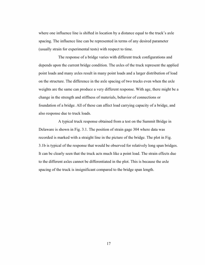
where one influence line is shifted in location by a distance equal to the truck’s axle
spacing. The influence line can be represented in terms of any desired parameter
(usually strain for experimental tests) with respect to time.
The response of a bridge varies with different truck configurations and
depends upon the current bridge condition. The axles of the truck represent the applied
point loads and many axles result in many point loads and a larger distribution of load
on the structure. The difference in the axle spacing of two trucks even when the axle
weights are the same can produce a very different response. With age, there might be a
change in the strength and stiffness of materials, behavior of connections or
foundation of a bridge. All of these can affect load carrying capacity of a bridge, and
also response due to truck loads.
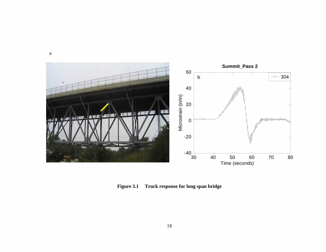
A typical truck response obtained from a test on the Summit Bridge in
Delaware is shown in Fig. 3.1. The position of strain gage 304 where data was
recorded is marked with a straight line in the picture of the bridge. The plot in Fig.
3.1b is typical of the response that would be observed for relatively long span bridges.
It can be clearly seen that the truck acts much like a point load. The strain effects due
to the different axles cannot be differentiated in the plot. This is because the axle
spacing of the truck is insignificant compared to the bridge span length.
-40
-20
0
20
40
60
30 40 50 60 70 80
Summit_Pass 2
304
Mic
rost
rain
(in/
in)
Time (seconds)
b
Figure 3.1 Truck response for long span bridge
18
a

19
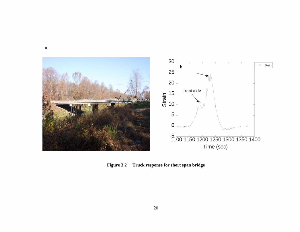
A typical response to a moving truck on a short-span bridge is shown in
Fig. 3.2b. The plot shows the truck response from the load test on Bridge 2_063 in
South Dover, DE (Fig. 3.2a). The truck response in this case is significantly affected
by the ratio of the axle weights and axle spacing. The effect of each axle in the truck
response (Fig. 3.2b) is easily seen. The greater the axle spacing, the more distinct is
the effect of each axle. The first small hump in the truck response shows the effect of
the first axle of the truck (i.e. when only the first axle is on the bridge). The hump
starts to decrease as the front axle moves away from mid-span. The larger second
hump in the truck response shows the effect of the second axle moving onto the
bridge. The maximum response usually occurs when the centroid of the two axles is at
mid-span. The response then decreases as the truck moves off the bridge. Thus, the
truck response is the summation of the two axles of the truck shifted by the axle
distance.
-5
0
5
10
15
20
25
30
1100 1150 1200 1250 1300 1350 1400
Strain
Stra
in
Time (sec)
b
front axle
Figure 3.2 Truck response for short span bridge
20
a
3.3 Theoretical example
The response in long span bridges can be simply taken as the effect of a
point load as discussed in the Truck Response section. In such cases, it is easy to get
the unit strain influence line. The truck response, when divided by the magnitude of
the total truck weight, becomes the unit strain influence line. For short and medium
span bridges (less than 80 ft.), typical trucks having axle spacing of 12 ft. can not be
considered point loads. The effects of both the front and rear axles of the vehicle can
be distinctly seen as shown in Fig. 3.2b. To distinguish the effect of a single axle,
strategic testing and appropriate mathematical manipulations of the response data is
necessary. By doing so, one can get a true experimental influence line.
Eliminating the effect of one of the two axles from the truck response will
yield the effect due to a single axle. However, the reduction of a two-axled response
into a single-axled response requires some manipulation. A simple numerical example
is presented here which illustrates the method of deriving the influence line from two-
axle truck effects. After the numerical example is presented, a case study using an
actual field test will be presented.
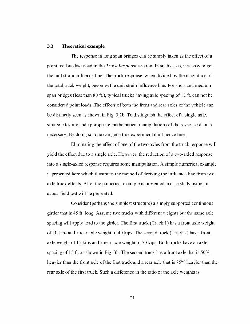
Consider (perhaps the simplest structure) a simply supported continuous
girder that is 45 ft. long. Assume two trucks with different weights but the same axle
spacing will apply load to the girder. The first truck (Truck 1) has a front axle weight
of 10 kips and a rear axle weight of 40 kips. The second truck (Truck 2) has a front
axle weight of 15 kips and a rear axle weight of 70 kips. Both trucks have an axle
spacing of 15 ft. as shown in Fig. 3b. The second truck has a front axle that is 50%
heavier than the front axle of the first truck and a rear axle that is 75% heavier than the
rear axle of the first truck. Such a difference in the ratio of the axle weights is
21

important in the mathematical manipulation of the response data to get the single axle
effect.
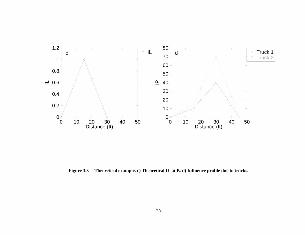
The continuous girder is supported at points A, B and C as shown in Fig.
3.3a. The reaction at support B is evaluated as a unit load moves from A to C (i.e. the
influence line for the reaction at B). From basic statics, the reaction at B due to a load
at any point on the girder can be calculated. Fig. 3.3c shows the influence line of the
reaction at support B. The reaction at B is equal to unity when the unit load is over B,
and varies linearly to zero as the load approaches the adjacent supports.
Now, consider the reaction at B due to the Trucks 1 and 2 as they move
across the girder, which are shown by the dashed and solid lines in Fig. 3.3d. This
response is obtained by superimposing the influence lines factored by the truck axle
weights and offset by the axle distance. These responses will be called influence
profiles because they are caused by the truck which has more than one axle. The
distance axis in the influence profile shows the position of the front axle of the truck
along the girder. Then the axle weights of the trucks need to be adjusted. To go from
an influence profile to an influence line, first the influence profile caused by Truck 1
with the front axle weight of 10 kips is amplified by the ratio of the front axle weights
of the two trucks (15 kips/10 kips = 1.5). This results in the response due to the
modified Truck 1 with front and rear axle weights of 15 kips and 60 kips, respectively.
Then this modified response is subtracted from the response due to Truck 2. Both
trucks now having equal front axle weights, the subtraction of the responses eliminates
the effect of the front axles of the trucks. The remaining response is then the response
due to a point load with the magnitude of the difference between the rear axle weights
of the two trucks (Fig. 3.3e). This response, when divided by the magnitude of the
22

resulting point load, gives the unit influence line. The offset in the distance axis of the
plot in Fig. 3.3e is due to the fact that the unit influence line is due to the unit rear axle
and the original influence profile plots are created according to the position of front
axle on the girder. To finish the process, the plot is shifted (by an amount equal to the
axle spacing) so that it represents the effect at B due to the location of the point load
which is now the rear axle of the trucks (Fig. 3.3f). Comparing Fig.’s 3.3c and 3.3f,
one can see that the influence line that was determined analytically for a single point
load is the same as the one found by manipulating the responses due to two trucks.
If the initial plots had been made according to the rear axle location, no
shifting of the plot is required. Also, if the ratio of the rear axle weights of the trucks
was used to factor the first truck (i.e. 70 kips/40 kips = 1.75), the factored first truck
will have the front axle weight of 17.5 kips and rear axle weight of 70 kips.
Subtracting the influence profiles of the two trucks will cancel out the rear axle effect
(both being 70 kips) and the result would be due to the difference of the front axle
weights of the two trucks (17.5 kips-15 kips = 2.5 kips). Dividing this subtracted
influence profile by the magnitude 2.5 would give the unit influence line due to the
front axle weight. In this case, since the distance axis is based on the front axle
position, the resulting influence line will not need an offset correction.
It can be seen that by using this process, the effect of a unit load can be
created using the effect of two trucks that have the same axle spacing but different
weights. For this method to work, the two trucks must have different ratios of front to
rear axle weights, and the truck axle spacings need to be the same. If not, either the
two trucks will cancel each other out completely, or the effect of one of the truck axles
23

24
will leave the remaining axle at a different location and the response to a single point
load will be obtained.
a
CBA
22.5 ft.22.5 ft.
70 kips 15 kips
40 kips 10 kips
Truck 1 Truck 2
b
Axle Spacing = 15 ft.
Figure 3.3 Theoretical example. a) Bridge geometry. b) Truck configuration.
25
0
0.2
0.4
0.6
0.8
1
1.2
0 10 20 30 40 50
ILIL
Distance (ft)
c
0
10
20
30
40
50
60
70
80
0 10 20 30 40 50
Truck 1Truck 2
IP
Distance (ft)
d
Figure 3.3 Theoretical example. c) Theoretical IL at B. d) Influence profile due to trucks.
26

27
0
2
4
6
8
10
0 10 20 30 40 50
12ILe
IL
Distance (ft)
0
0.2
0.4
0.6
0.8
1
0 10 20 30 40 50
IL
Distance (ft)
1.2Final ILf
Figure 3.3 Theoretical example. e) IL derived after subtraction of IP’s. f) Final IL after offsetting distance.

28
Chapter 4
EXPERIMENTAL APPROACH
4.1 Test case
An experimental influence line provides the actual effect of a moving load
crossing a bridge. The influence line obtained from the load test can be used for bridge
management to efficiently determine the allowable loads and safe carrying capacity of
the bridge, and to evaluate load distribution. Typically, the truck load as a whole is
considered when evaluating load capacity regardless of the trucks axle spacings. The
experimental influence line test requires a service truck to be run over the bridge in a
specific pattern. Strain gages are fixed at those locations on the bridge where the
influence line is desired. The selection of such locations needs careful attention.
Usually, the location where maximum response is expected is a good choice.

Figure 4.1 South market street bridge
29
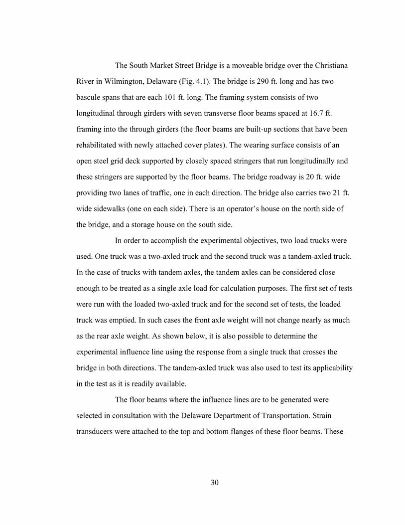
The South Market Street Bridge is a moveable bridge over the Christiana
River in Wilmington, Delaware (Fig. 4.1). The bridge is 290 ft. long and has two
bascule spans that are each 101 ft. long. The framing system consists of two
longitudinal through girders with seven transverse floor beams spaced at 16.7 ft.
framing into the through girders (the floor beams are built-up sections that have been
rehabilitated with newly attached cover plates). The wearing surface consists of an
open steel grid deck supported by closely spaced stringers that run longitudinally and
these stringers are supported by the floor beams. The bridge roadway is 20 ft. wide
providing two lanes of traffic, one in each direction. The bridge also carries two 21 ft.
wide sidewalks (one on each side). There is an operator’s house on the north side of
the bridge, and a storage house on the south side.
In order to accomplish the experimental objectives, two load trucks were
used. One truck was a two-axled truck and the second truck was a tandem-axled truck.
In the case of trucks with tandem axles, the tandem axles can be considered close
enough to be treated as a single axle load for calculation purposes. The first set of tests
were run with the loaded two-axled truck and for the second set of tests, the loaded
truck was emptied. In such cases the front axle weight will not change nearly as much
as the rear axle weight. As shown below, it is also possible to determine the
experimental influence line using the response from a single truck that crosses the
bridge in both directions. The tandem-axled truck was also used to test its applicability
in the test as it is readily available.
The floor beams where the influence lines are to be generated were
selected in consultation with the Delaware Department of Transportation. Strain
transducers were attached to the top and bottom flanges of these floor beams. These
30

31
strain transducers were connected to an automated data acquisition system that
recorded strain data with respect to time as the trucks crossed the bridge. The trucks
were driven across the bridge one at a time at a slow and constant speed (about 1
ft/sec) and the strain data was recorded. Traffic was not allowed on the bridge at the
time when the test truck was passing over it. The automated system was set to record
the strain data at every 0.05 secs.
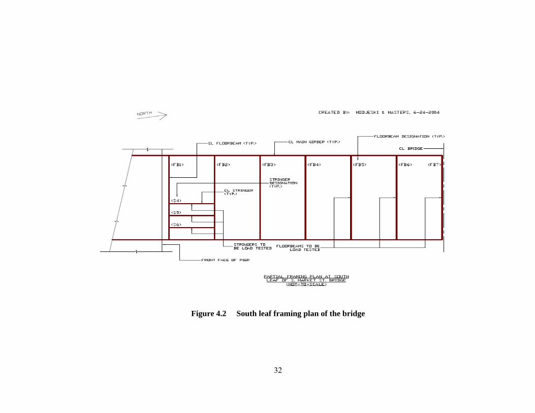
Figure 4.2 South leaf framing plan of the bridge
32

33
For this specific test, the floor beams of the south leaf of the South Market
Street Bridge were instrumented. Each bascule span has seven floor beams. In the
south leaf, it is noted that the southern most floor beam is floor beam 1 (FB1) and the
northern most one is FB7, as shown in Fig. 4.2. Gages 346 and 355 (each transducer
has a three-digit identification number) were attached to the second floor beam (FB2),
Gages 303, 342, and 318 were attached to FB3, and Gages 317, 348, and 338 were
attached to FB4. These gages are attached to the flanges of the floor beams by clamps.
Gages 317 and 348, attached to the bottom flange of FB4, are shown in Fig. 6. Gages
318 and 338 were attached to the top flanges of the floor beams and thus negative
strain is expected in these two gages when the truck passes over the bridge. Positive
strain is expected in the bottom flanges and thus the rest of the gages during the test.
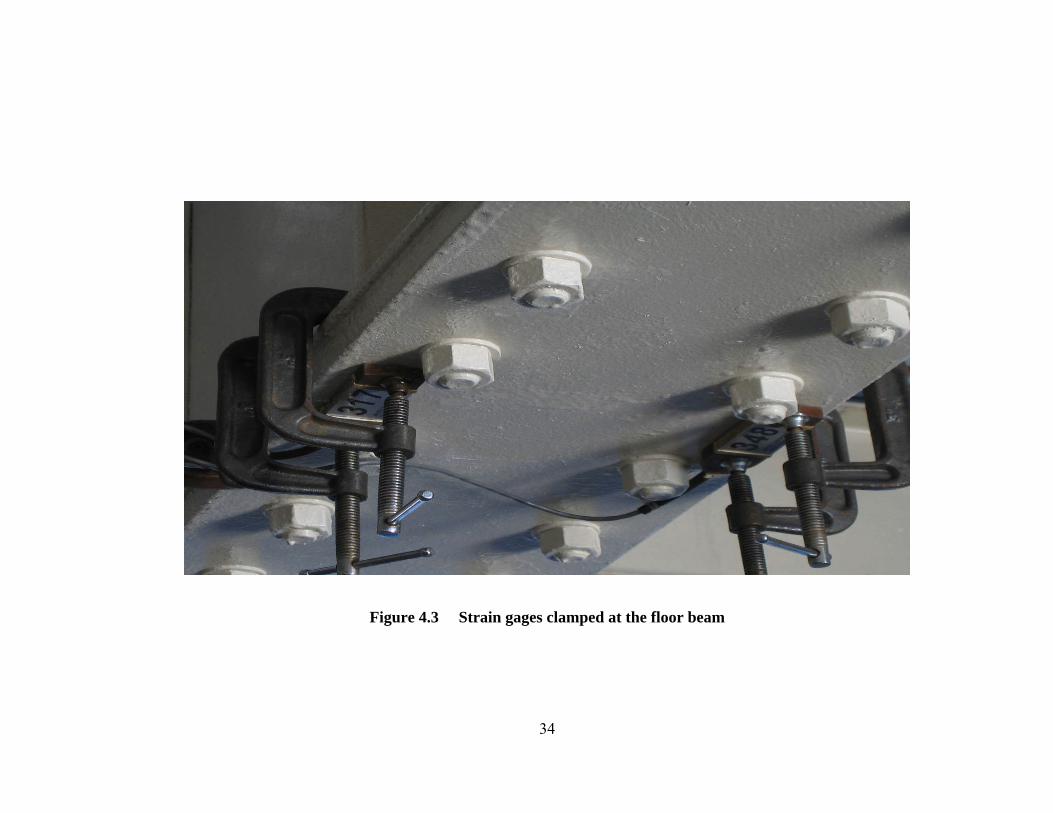
Figure 4.3 Strain gages clamped at the floor beam
34
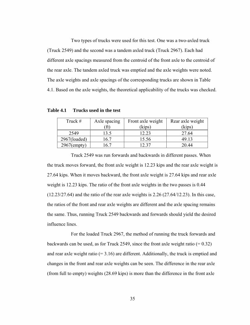
Two types of trucks were used for this test. One was a two-axled truck
(Truck 2549) and the second was a tandem axled truck (Truck 2967). Each had
different axle spacings measured from the centroid of the front axle to the centroid of
the rear axle. The tandem axled truck was emptied and the axle weights were noted.
The axle weights and axle spacings of the corresponding trucks are shown in Table
4.1. Based on the axle weights, the theoretical applicability of the trucks was checked.
Table 4.1 Trucks used in the test
Truck # Axle spacing (ft)
Front axle weight (kips)
Rear axle weight (kips)
2549 13.5 12.23 27.64 2967(loaded) 16.7 15.56 49.13 2967(empty) 16.7 12.37 20.44
Truck 2549 was run forwards and backwards in different passes. When
the truck moves forward, the front axle weight is 12.23 kips and the rear axle weight is
27.64 kips. When it moves backward, the front axle weight is 27.64 kips and rear axle
weight is 12.23 kips. The ratio of the front axle weights in the two passes is 0.44
(12.23/27.64) and the ratio of the rear axle weights is 2.26 (27.64/12.23). In this case,
the ratios of the front and rear axle weights are different and the axle spacing remains
the same. Thus, running Truck 2549 backwards and forwards should yield the desired
influence lines.
For the loaded Truck 2967, the method of running the truck forwards and
backwards can be used, as for Truck 2549, since the front axle weight ratio (= 0.32)
and rear axle weight ratio (= 3.16) are different. Additionally, the truck is emptied and
changes in the front and rear axle weights can be seen. The difference in the rear axle
(from full to empty) weights (28.69 kips) is more than the difference in the front axle
35
weights (3.19 kips) because of the nature of the truck geometry. The ratio of the front
and rear axle weights of the loaded and the emptied trucks were 1.26 and 2.40
respectively. Thus, the same truck can be used, with one pass being fully loaded and
the other being empty. This has the advantage of running the truck forwards in both
passes but the disadvantage of having to empty the truck.
4.2 Testing procedure
When the test trucks were passing over the bridge all traffic was stopped
for a short while before the truck was run over the bridge and a short while after it
passed the bridge in order to avoid any interference on the strain data due to other
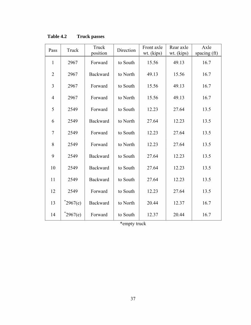
vehicles. Fourteen passes were conducted to investigate the sensitivity of the method
to various testing scenarios (see Table 4.2). In order to accomplish the desired goal of
having responses from trucks with different axle weights but the same axle spacing,
the trucks were driven across the bridge in one direction but with the truck running
forwards once and backwards the second time across the bridge (e.g. in the sixth pass,
the truck was traveling from south to north backwards and in the eighth pass it ran
forwards from south to north). Such positioning of the trucks causes the front and rear
axle weights to interchange and maintain the difference in the front and rear axle
weights as discussed in Test Case. The corresponding front and rear axle weights for
the pairs of passes used to compute the various influence lines are given in Table 4.2.
36
37
Table 4.2 Truck passes
Pass Truck Truck position Direction Front axle
wt. (kips) Rear axle wt. (kips)
Axle spacing (ft)
1 2967 Forward to South 15.56 49.13 16.7
2 2967 Backward to North 49.13 15.56 16.7
3 2967 Forward to South 15.56 49.13 16.7
4 2967 Forward to North 15.56 49.13 16.7
5 2549 Forward to South 12.23 27.64 13.5
6 2549 Backward to North 27.64 12.23 13.5
7 2549 Forward to South 12.23 27.64 13.5
8 2549 Forward to North 12.23 27.64 13.5
9 2549 Backward to South 27.64 12.23 13.5
10 2549 Backward to South 27.64 12.23 13.5
11 2549 Backward to South 27.64 12.23 13.5
12 2549 Forward to South 12.23 27.64 13.5
13 *2967(e) Backward to North 20.44 12.37 16.7
14 *2967(e) Forward to South 12.37 20.44 16.7
*empty truck
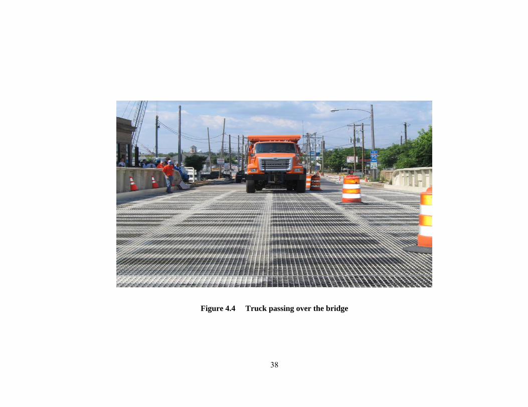
Figure 4.4 Truck passing over the bridge
38
Since the truck had different speeds at different intervals of time during a
single pass, a clicker was used to mark (in the data file) the time when the front axle of
the truck was over a specific floor beam. This was later used to determine the truck
speed from floor beam to floor beam. With these truck speeds the time scale was
changed into a distance scale. The time when the truck was between two floor beams
was multiplied by the speed of the truck between the two floor beams. Had the truck
traveled with a constant speed (which is not easy to accomplish), the time scale could
be easily converted to the distance scale with a single calculation.
The first test (not discussed in this study) was conducted with a truck
running forwards in one direction and then again in the opposite direction. The strains
from the two passes need to be compared at the same locations on the bridge. To make
the strains comparable, the time axis for one pass has to be flipped, which requires a
lot of computational effort and thus was not used.
4.3 Experimental example
Two sets of passes are considered here to verify the theoretical example
using experimental data. In particular, Passes 6 and 8 and Passes 7 and 10 are used.
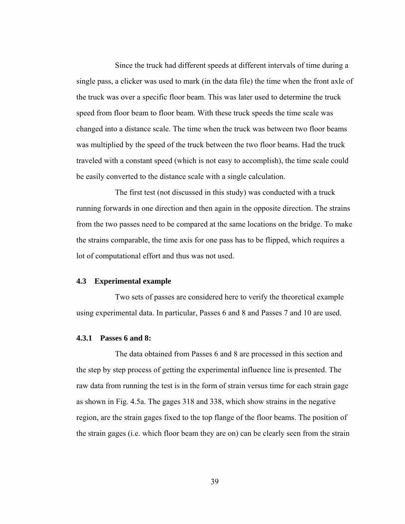
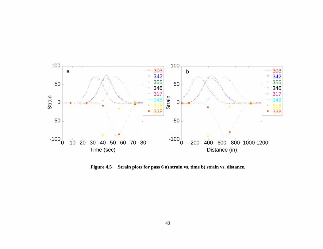
4.3.1 Passes 6 and 8:
The data obtained from Passes 6 and 8 are processed in this section and
the step by step process of getting the experimental influence line is presented. The
raw data from running the test is in the form of strain versus time for each strain gage
as shown in Fig. 4.5a. The gages 318 and 338, which show strains in the negative
region, are the strain gages fixed to the top flange of the floor beams. The position of
the strain gages (i.e. which floor beam they are on) can be clearly seen from the strain
39

data. Gages 355 and 346, having the peaks at the same time, are on the same floor
beam (FB2).
The time interval for recording data was 0.05 seconds. The time axis is
changed into the distance axis using the truck speed for ease of calculation and also
proper representation of an influence line. A sample calculation of the truck’s speed
for Pass 6 is shown in Table 4.3. The clicker time denotes the time when the truck had
its front axle right above each of the floor beams. The clicker times obtained from the
system are in whole numbers which were then multiplied by 0.05 to get the time of the
clicker in seconds as shown in the second column of Table 4.2. The time interval of
the truck remaining between two consecutive floor beams during the test was
calculated in column 3 in Table 4.3. The distance between the floor beams (201.5
inches for all floor beams) was divided by the time intervals. This gives the average
speed of the truck between the two corresponding floor beams.
40

Table 4.3 Calculation of truck speed.
Clicker times
Time (sec)
Interval (sec)
Average speed (ft/sec)
0 0.00
369 18.45 18.45 0.91
594 29.70 11.25 1.49
834 41.70 12.00 1.39
1014 50.70 9.00 1.86
1259 62.95 12.25 1.37
1460 73.00 10.05 1.67
1653 82.65 9.65 1.74
As seen from Table 4.3, the truck moves very slowly (approximately 1.5
ft/sec). In this table, eight clicker times are shown. The clicker time 0 refers to the
time the test was started and the clicker time 369 is the time when the truck is over
FB1 or it can be said that the truck moves onto the bridge at this time. The time
interval and speed between 0 and 369 would have no significance as the truck is not
yet on the bridge. The clicker time 1653 denotes the time when the truck is over FB7
and the corresponding speed is that of the truck between FB6 and FB7. A constant
speed of the truck would have been preferred for the ease of computation; however
this will not always be possible. If this can be accomplished, the speed of the truck
when multiplied by the time in the raw data would directly become the distance on the
bridge where the front axle is loaded. FB1 is taken as the base point, and the time
difference of a point after FB1 and the time at FB1 is multiplied by the truck speed
when it is between FB1 and FB2. The obtained distance is then added to the distance
of FB1. The same process continues as the truck crosses each floor beam. It is
41
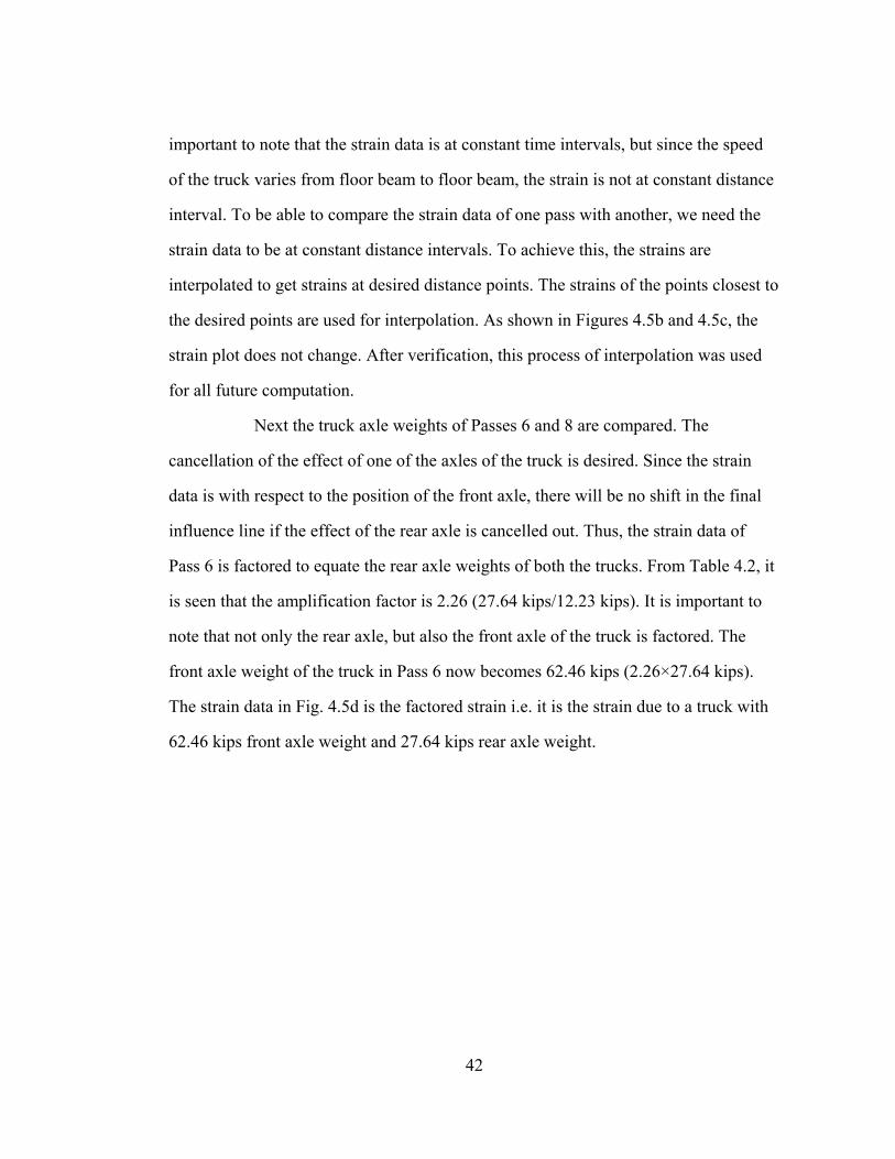
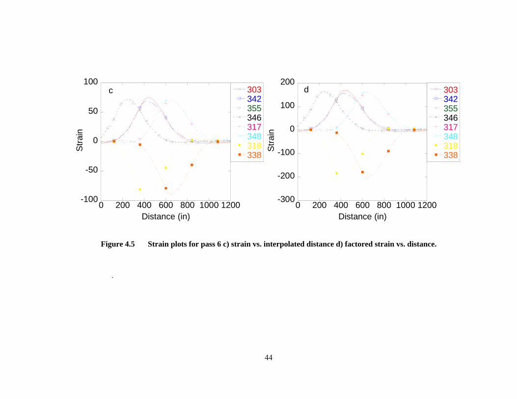
42
important to note that the strain data is at constant time intervals, but since the speed
of the truck varies from floor beam to floor beam, the strain is not at constant distance
interval. To be able to compare the strain data of one pass with another, we need the
strain data to be at constant distance intervals. To achieve this, the strains are
interpolated to get strains at desired distance points. The strains of the points closest to
the desired points are used for interpolation. As shown in Figures 4.5b and 4.5c, the
strain plot does not change. After verification, this process of interpolation was used
for all future computation.
Next the truck axle weights of Passes 6 and 8 are compared. The
cancellation of the effect of one of the axles of the truck is desired. Since the strain
data is with respect to the position of the front axle, there will be no shift in the final
influence line if the effect of the rear axle is cancelled out. Thus, the strain data of
Pass 6 is factored to equate the rear axle weights of both the trucks. From Table 4.2, it
is seen that the amplification factor is 2.26 (27.64 kips/12.23 kips). It is important to
note that not only the rear axle, but also the front axle of the truck is factored. The
front axle weight of the truck in Pass 6 now becomes 62.46 kips (2.26×27.64 kips).
The strain data in Fig. 4.5d is the factored strain i.e. it is the strain due to a truck with
62.46 kips front axle weight and 27.64 kips rear axle weight.
-100
-50
0
50
100
0 10 20 30 40 50 60 70 80
303342355346317348318338
Stra
in
Time (sec)
a
-100
-50
0
50
100
0 200 400 600 800 1000 1200
303342355346317348318338
Stra
in
Distance (in)
b
Figure 4.5 Strain plots for pass 6 a) strain vs. time b) strain vs. distance.
43
-100
-50
0
50
100
0 200 400 600 800 1000 1200
303342355346317348318338
Stra
in
Distance (in)
c
-300
-200
-100
0
100
200
0 200 400 600 800 1000 1200
303342355346317348318338
Stra
in
Distance (in)
d
Figure 4.5 Strain plots for pass 6 c) strain vs. interpolated distance d) factored strain vs. distance.
44
.
45
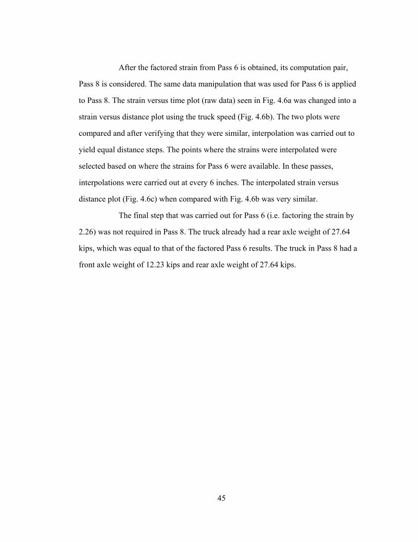
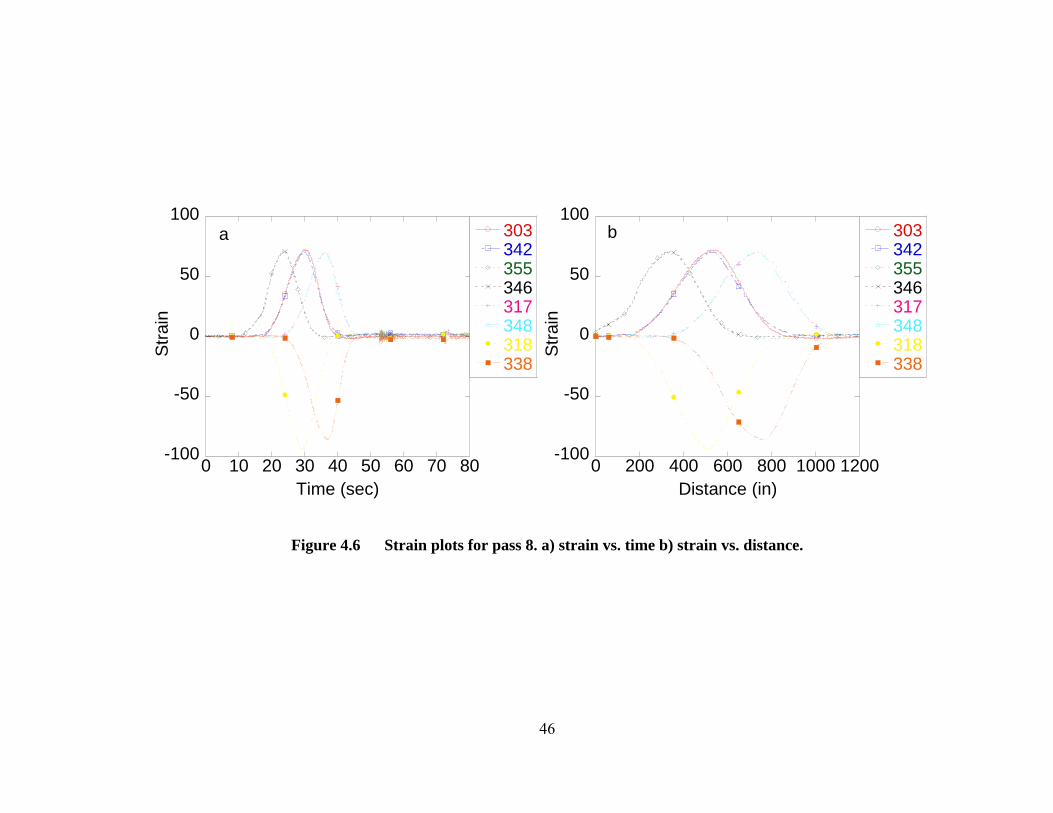
After the factored strain from Pass 6 is obtained, its computation pair,
Pass 8 is considered. The same data manipulation that was used for Pass 6 is applied
to Pass 8. The strain versus time plot (raw data) seen in Fig. 4.6a was changed into a
strain versus distance plot using the truck speed (Fig. 4.6b). The two plots were
compared and after verifying that they were similar, interpolation was carried out to
yield equal distance steps. The points where the strains were interpolated were
selected based on where the strains for Pass 6 were available. In these passes,
interpolations were carried out at every 6 inches. The interpolated strain versus
distance plot (Fig. 4.6c) when compared with Fig. 4.6b was very similar.
The final step that was carried out for Pass 6 (i.e. factoring the strain by
2.26) was not required in Pass 8. The truck already had a rear axle weight of 27.64
kips, which was equal to that of the factored Pass 6 results. The truck in Pass 8 had a
front axle weight of 12.23 kips and rear axle weight of 27.64 kips.
-100
-50
0
50
100
0 10 20 30 40 50 60 70 80
303342355346317348318338
Stra
in
Time (sec)
a
-100
-50
0
50
100
0 200 400 600 800 1000 1200
303342355346317348318338
Stra
in
Distance (in)
b
Figure 4.6 Strain plots for pass 8. a) strain vs. time b) strain vs. distance.
46
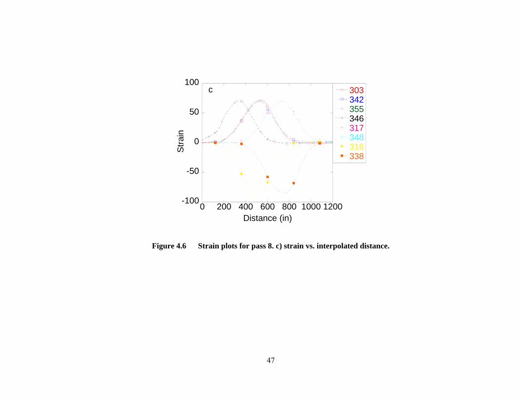
Figure 4.6 Strain plots for pass 8. c) strain vs. interpolated distance.
-100
-50
0
50
100
0 200 400 600 800 1000 1200
303342355346317348318338
Stra
in
Distance (in)
c
47

48
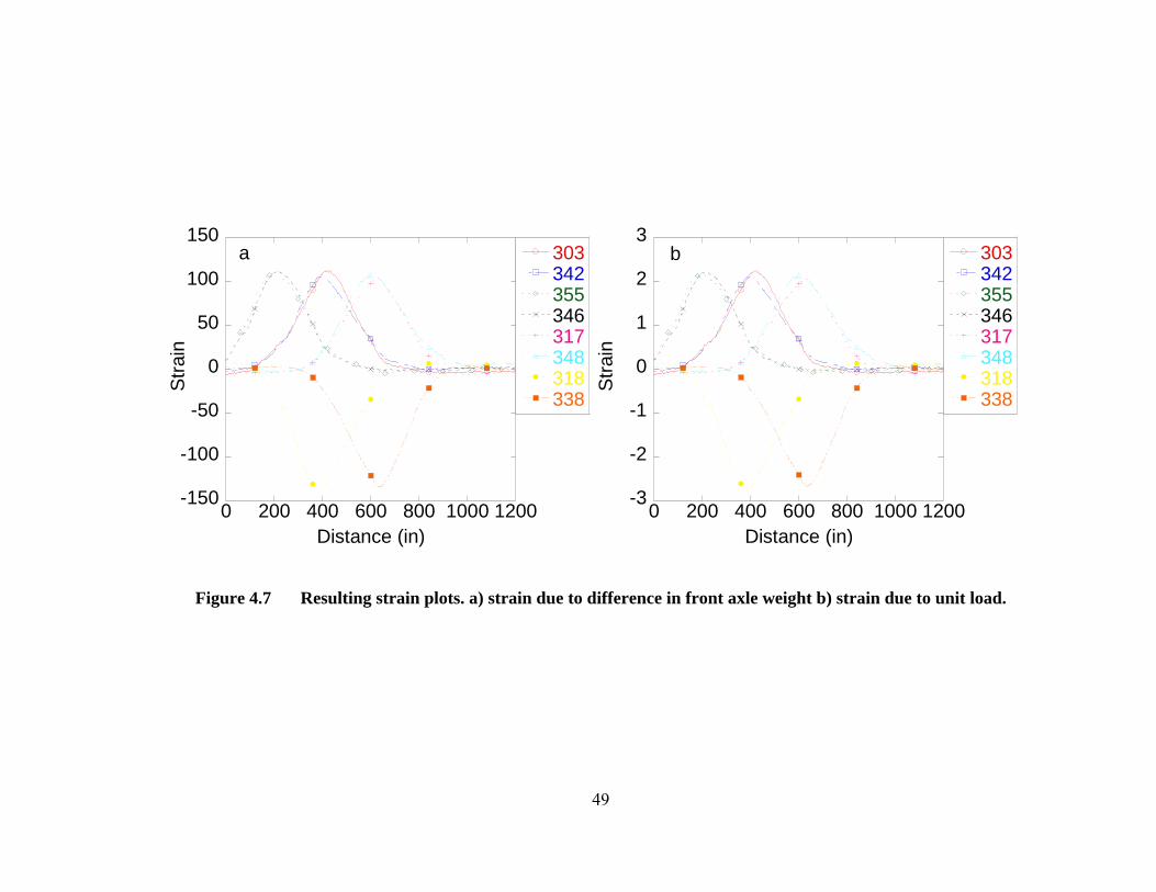
The adjusted strain data for both Pass 6 and Pass 8 versus distance are
shown in Figures 4.5d and 4.6c. By subtracting the strains from Pass 8 from the strains
of the factored Pass 6, the strain due to a single axle load was obtained. This axle load
had the magnitude equal to the difference between the front axles of the trucks in
Passes 6 and 8 i.e. 50.23 kips (= 62.46-12.23 kips). The resulting plot is shown in Fig.
4.7a. This response was then divided by the magnitude 50.23 to get the strain due to a
unit point load i.e. the experimental strain influence line.
-150
-100
-50
0
50
100
150
0 200 400 600 800 1000 1200
303342355346317348318338
Stra
in
Distance (in)
a
-3
-2
-1
0
1
2
3
0 200 400 600 800 1000 1200
303342355346317348318338
Stra
in
Distance (in)
b
Figure 4.7 Resulting strain plots. a) strain due to difference in front axle weight b) strain due to unit load.
49

50
4.3.2 Passes 7 and 10:
Passes 7 and 10 are more unconventional stopping passes (i.e. during the
test, the trucks were stopped for a brief time at certain locations as the truck crossed
the bridge). In Passes 7 and 10, the trucks were stopped at every third point between
the floor beams (at every 5.6 ft.). From the plot in Fig. 4.8a, the time at which the
truck stopped can be easily identified. The strains remain the same for a short time
when the truck is stopped as indicated by the horizontal portions of the strain plot.
Thus, both the time and the distance at which the truck stopped are known. The strains
at those particular times, as obtained from the raw data, were then plotted against the
known locations on the bridge (Fig. 4.8b). Here again, the distance refers to the
location of the front axle of the truck on the bridge. The strain-distance plot is shown
in Fig. 4.8b as a stepped plot because of the discontinuity of the strain data. One
should note that in this case, the strain data is at larger intervals of distance as
compared to Passes 6 and 8.
The strain data for Pass 10 was then factored in a similar way to what was
done for Pass 6. After factoring (by a factor of 2.26), the resulting strain would be that
due to a truck with a front axle weight of 62.46 kips and a rear axle weight of 27.64
kips. This strain response is shown in Fig. 4.8c.

-100
-50
0
50
100
0 50 100 150 200 250 300
303342355346317348318338S
train
Time (sec)
a
-100
-50
0
50
100
0 200 400 600 800 1000 1200
303342355346317348318338S
train
Distance (in)
b
Figure 4.8 Strain plots for pass 10. a) strain vs. time b) strain vs. distance.
51

Figure 4.8 Strain plots for pass 10. c) factored strain vs. distance.
-300
-200
-100
0
100
200
0 200 400 600 800 1000 1200
342303355346348317318338St
rain
Distance (in)
c
52

53
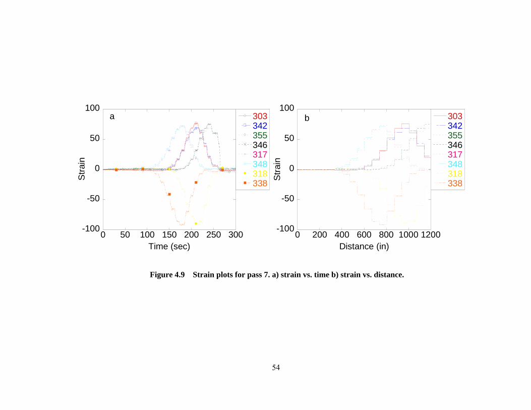
In Pass 7, the truck was again stopped at every point between floor beams.
Knowing this, the strain versus distance plot (Fig. 4.9b) for Pass 7 was obtained from
the strain-time plot (Fig. 4.9a). This is also a step-graph representation as shown in
Fig. 4.9b. The truck used in Pass 7 had a front axle weight of 12.23 kips and a rear
axle weight of 27.64kips.
The truck was stopped for a short while at the same locations in Pass 7 as
was in Pass 10. The strains in both passes were recorded with the truck at the same
location, and thus, there was no need to interpolate the strain data as was done for
Passes 6 and 8.
-100
-50
0
50
100
0 50 100 150 200 250 300
303342355346317348318338S
train
Time (sec)
a
-100
-50
0
50
100
0 200 400 600 800 1000 1200
303342355346317348318338S
train
Distance (in)
b
Figure 4.9 Strain plots for pass 7. a) strain vs. time b) strain vs. distance.
54

55
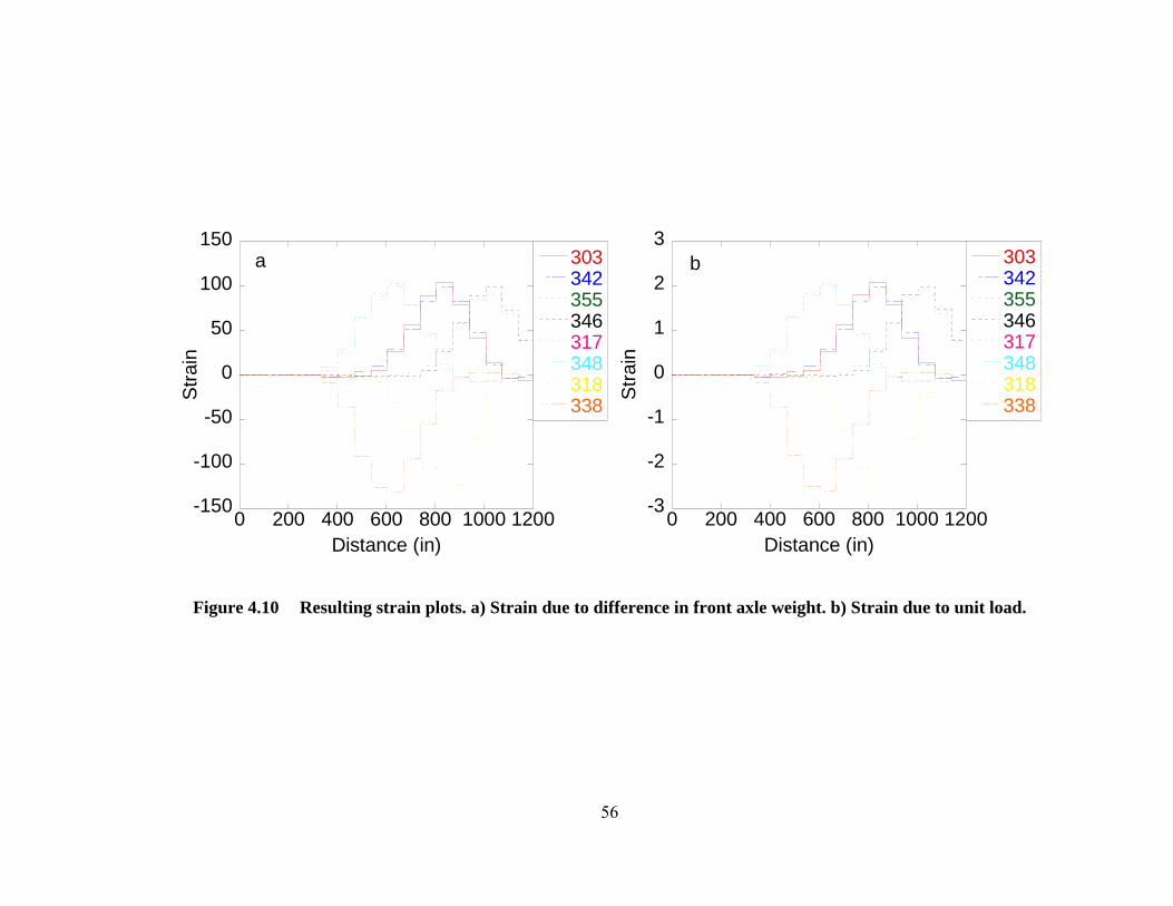
The strains from Pass 7 were then subtracted from the factored strains
from Pass 10 (Fig. 4.10a). The difference between the front axle weights of the trucks
in Pass 7 and factored Pass 10 was 50.23 kips. Figure 4.10a shows the strain due to a
point load of magnitude 50.23 kips. This response, when divided by 50.23, gives the
strain due to unit load as seen in Fig. 4.10b. To compare the results of this pass with
the continuous type results, a continuous line plot is drawn taking the mid-point of the
steps and joining them (this can be done using many types of software). This is shown
in Fig. 4.10c. It can be seen that the resulting plot is very similar to the experimental
strain influence line obtained from Passes 6 and 8 (Fig. 4.7b). This verifies the use of
the stopping technique in experimental influence line testing is appropriate.
A clear advantage of this stopping technique would be less computational
effort. The truck speed does not need to be calculated since the location of the truck is
known and so is the time when it was stopped. Furthermore, the location is the same
for both passes. The strains at these points are comparable and the strain versus time
plot can be easily changed into the strain versus distance plot. This method also
completely avoids the need of interpolation, which is the most tedious job in the other
method (as seen in Passes 6 and 8).
-150
-100
-50
0
50
100
150
0 200 400 600 800 1000 1200
303342355346317348318338S
train
Distance (in)
a
-3
-2
-1
0
1
2
3
0 200 400 600 800 1000 1200
303342355346317348318338S
train
Distance (in)
b
Figure 4.10 Resulting strain plots. a) Strain due to difference in front axle weight. b) Strain due to unit load.
56
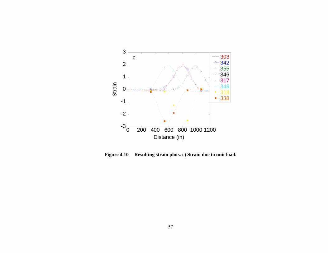
Figure 4.10 Resulting strain plots. c) Strain due to unit load.
-3
-2
-1
0
1
2
3
0 200 400 600 800 1000 1200
303342355346317348318338S
train
Distance (in)
c
57
Chapter 5
EXPERIMENTAL INFLUENCE LINE
5.1 Test results
The various truck passes conducted during the South Market Bridge load
test shown in Table 4.2 were paired up for computational purposes depending on their
direction and front and rear axle weights. The pairs are shown below:-
Passes 7 and 10, Passes 6 and 8, Passes 5 and 9, Passes 11 and 12, Passes
3 and14, Passes 1 and 14, Passes 4 and 13, Passes 2 and 4, and Passes 2 and 13.
The pair of Passes 6 and 8 represents the typical example of using a single
truck to derive the experimental influence line. The truck was run backwards in Pass 6
and forwards in Pass 8, both going northwards. As a result, different front and rear
axle weights in the two passes using a single truck were obtained. As alluded to earlier
in Chapter 4 (Passes 6 and 8), inverting the truck orientation gave different axle
weights and also different ratios of the axle weights of the trucks in the two passes
while using the same truck. Passes 5 and 9 and Passes 2 and 4 are the same. Tandem
axle trucks were used in Passes 2 and 4. Passes 11 and 12 involved tests carried out on
the east side of the bridge in which the truck’s longitudinal axis was shifted
approximately 2 ft. from the center towards the east side. Passes 7 and 10 were the
only different types of passes conducted (used the stopping method). This method, as
described, has a number of advantages over the other methods. Passes 13 and 14
58

59
included the empty tandem axled trucks and showed a lot of noise in the strain data as
will be seen later (likely due to the low truck weight).
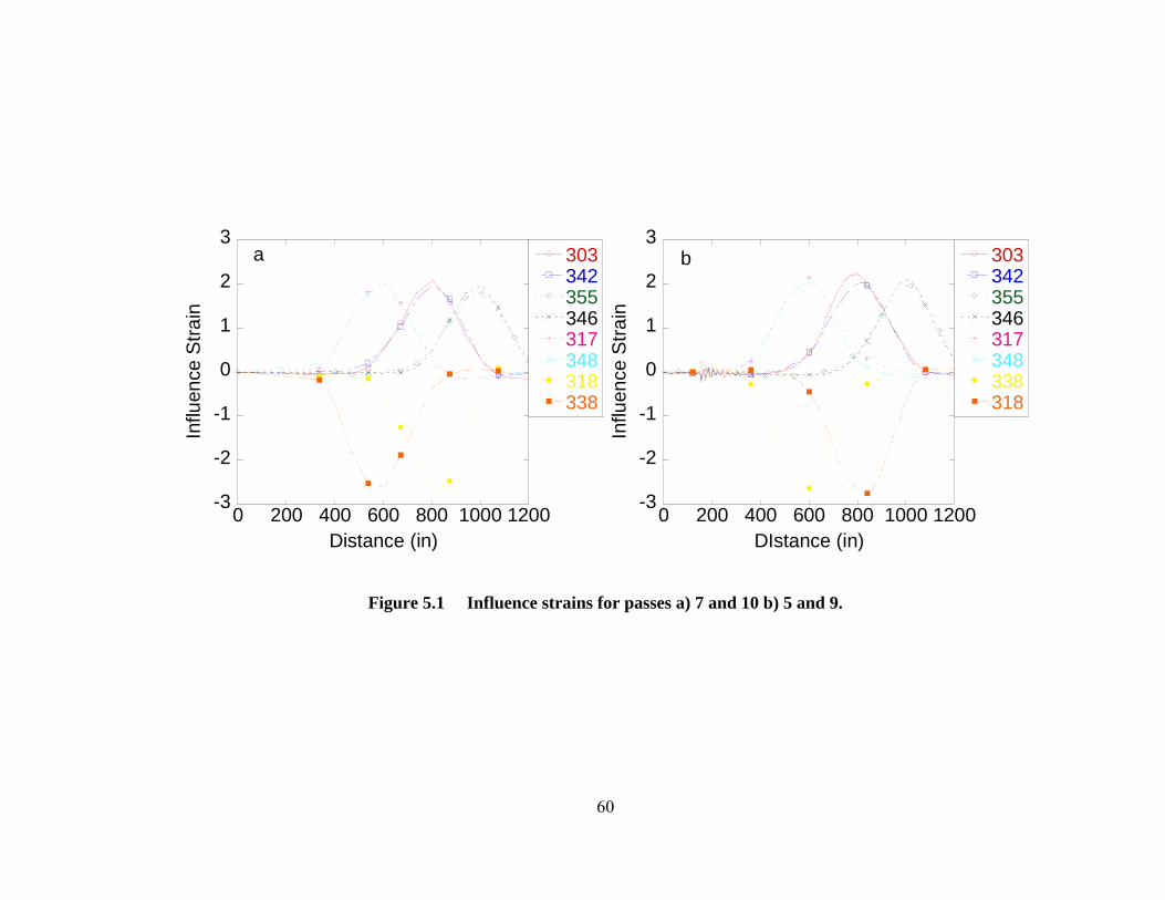
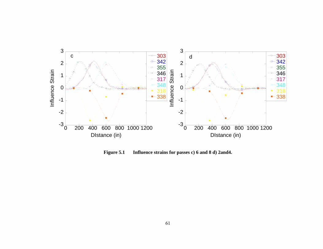
Experimental strain influence lines were derived for all pairs of passes
using the methodology presented in Chapter 4. The strain influence lines for all the
gages obtained for the pairs 7 and 10, 6 and 8, 5 and 9, and 2 and 4 are shown in Fig.
5.1.
-3
-2
-1
0
1
2
3
0 200 400 600 800 1000 1200
303342355346317348318338
Influ
ence
Stra
in
Distance (in)
a
-3
-2
-1
0
1
2
3
0 200 400 600 800 1000 1200
303342355346317348338318
Influ
ence
Stra
in
DIstance (in)
b
Figure 5.1 Influence strains for passes a) 7 and 10 b) 5 and 9.
60
-3
-2
-1
0
1
2
3
0 200 400 600 800 1000 1200
303342355346317348318338
Influ
ence
Stra
in
DIstance (in)
c
-3
-2
-1
0
1
2
3
0 200 400 600 800 1000 1200
303342355346317348318338
Influ
ence
Stra
in
DIstance (in)
d
Figure 5.1 Influence strains for passes c) 6 and 8 d) 2and4.
61
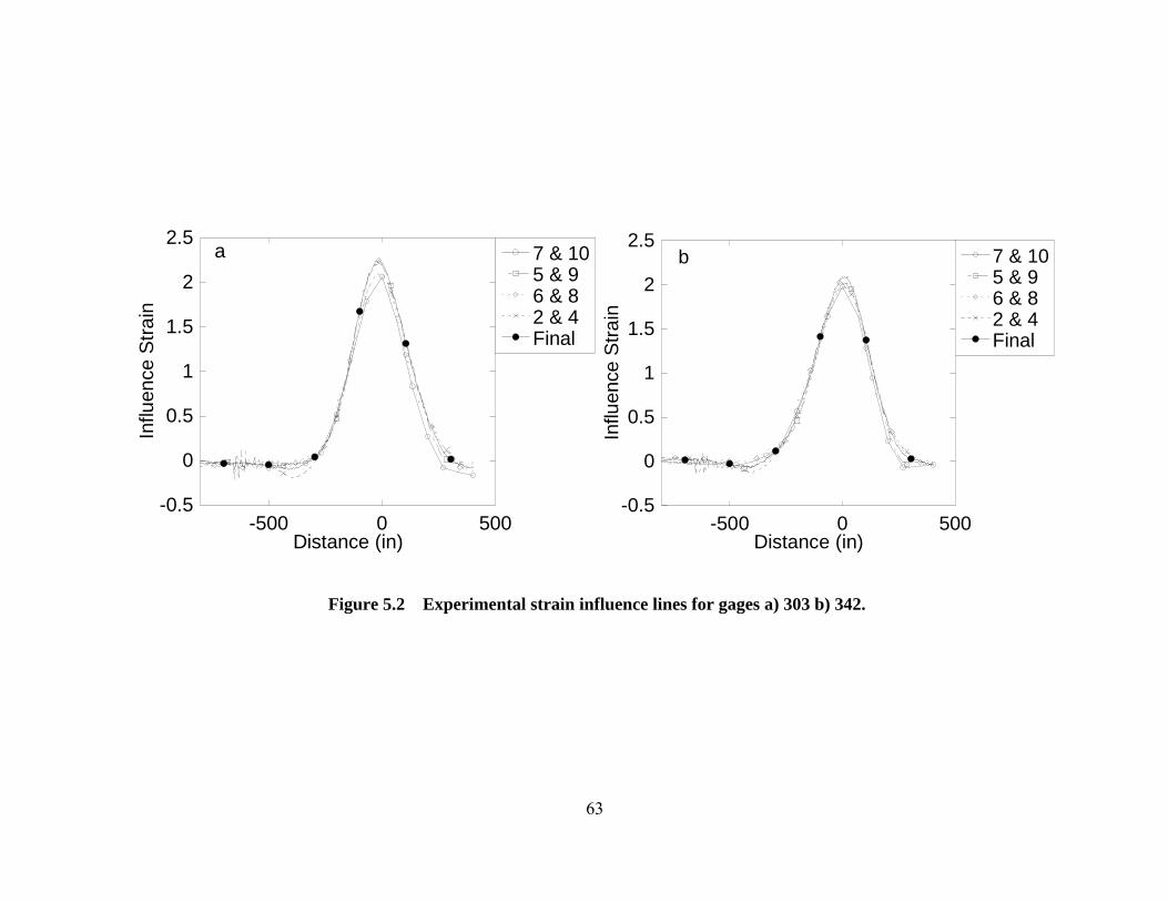
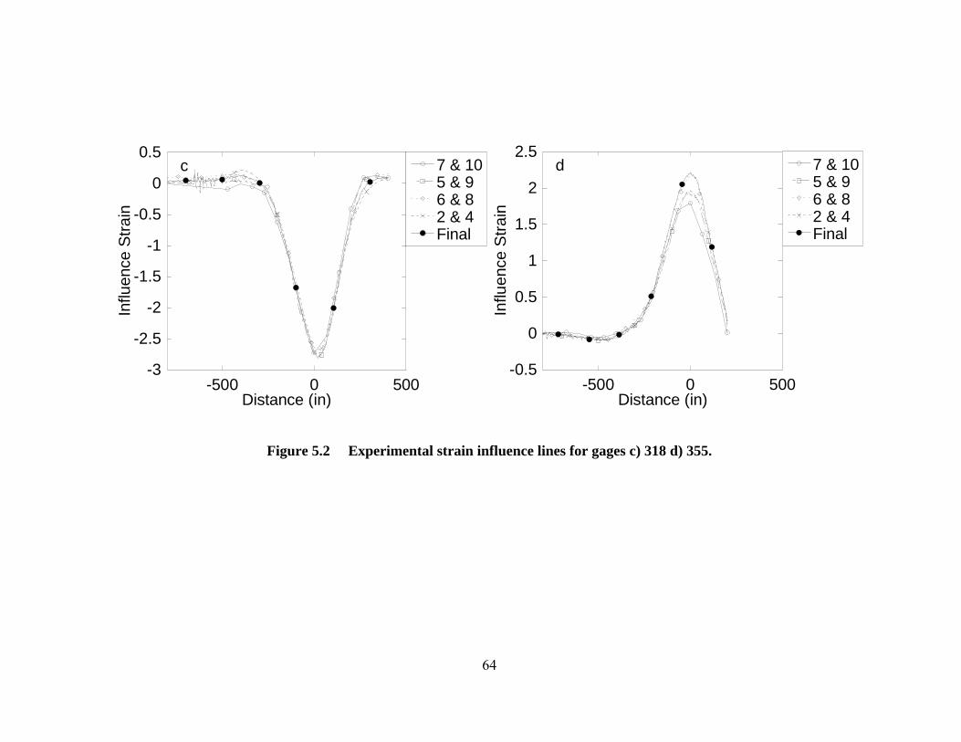
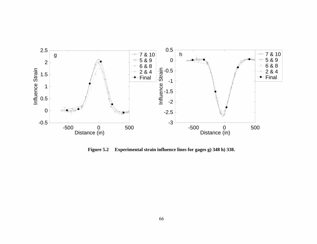
The final strain influence lines along with the strain influence lines
obtained from each of the pairs of passes (including Passes 7 and 10, represented in
straight lines) are shown in Fig. 5.2.
The final strain influence lines for all gage locations were calculated by
averaging of all the strain influence lines. The strain influence lines obtained from
Passes 7 and 10 were excluded in the calculation of final strain influence line. The
strain influence line obtained from Passes 7 and 10 was not included in taking the
average because it is segmental (Fig. 4.10b). The final strain influence line was
calculated as the average of all the strain influence lines and factored such that the
final strain influence line would equal the maximum strain due to unit load obtained in
the individual strain influence lines. This can be simply written as:
5.2 Influence lines for gage locations
Note that the truck traveled northwards in Passes 7, 10, 5 and 9 and it
traveled southwards in Passes 6, 8, 2 and 4. This explains the reason why the strain
plots are shifted to left in Figures 5.1c and 5.1d. The distance axis represents the entire
length of the bascule span of the bridge which is 1,209 inches. If we look at gage 348,
which is in FB4, in all the four plots in Fig. 5.1, it is on the left in the first two plots
and is on the right on the next two plots. In Passes 7, 10, 5 and 9, the truck approached
FB4 first, passed it and went over FB3 and then FB2. In Passes 6, 8, 2 and 4, the truck
passed in the opposite direction, passing over FB2, then FB3 and in the end FB4. The
individual strain influence lines for each gage are very similar in all cases.
average theof maximumstrains all of valuemaximum strains all of average strain Final ×=
62
-0.5
0
0.5
1
1.5
2
2.5
-500 0 500
7 & 105 & 96 & 82 & 4Final
Influ
ence
Stra
in
Distance (in)
a
-0.5
0
0.5
1
1.5
2
2.5
-500 0 500
7 & 105 & 96 & 82 & 4Final
Influ
ence
Stra
in
Distance (in)
b
Figure 5.2 Experimental strain influence lines for gages a) 303 b) 342.
63
-3
-2.5
-2
-1.5
-1
-0.5
0
0.5
-500 0 500
7 & 105 & 96 & 82 & 4Final
Influ
ence
Stra
in
Distance (in)
c
-0.5
0
0.5
1
1.5
2
2.5
-500 0 500
7 & 105 & 96 & 82 & 4Final
Influ
ence
Stra
in
Distance (in)
d
Figure 5.2 Experimental strain influence lines for gages c) 318 d) 355.
64

-0.5
0
0.5
1
1.5
2
2.5
-500 0 500
7 & 105 & 96 & 82 & 4Final
Influ
ence
Stra
in
Distance (in)
e
-0.5
0
0.5
1
1.5
2
2.5
-500 0 500
7 & 105 & 96 & 82 & 4Final
Influ
ence
Stra
in
Distance (in)
f
Figure 5.2 Experimental strain influence lines for gages e) 346 f) 317.
65
-0.5
0
0.5
1
1.5
2
2.5
-500 0 500
7 & 105 & 96 & 82 & 4Final
Influ
ence
Stra
in
Distance (in)
g
-3
-2.5
-2
-1.5
-1
-0.5
0
0.5
-500 0 500
7 & 105 & 96 & 82 & 4Final
Influ
ence
Stra
in
Distance (in)
h
Figure 5.2 Experimental strain influence lines for gages g) 348 h) 338.
66

As can be seen in Fig. 5.2, the peak values for all strain gages are almost
the same. These peak values are governed by the beam properties.
From Hooke’s law,
εEσ ×= (1)
IzMσ ×= (2)
where,
σ = stress at a location z from the neutral axis.
E = Young’s modulus of elasticity for the material.
ε = strain at a distance z from the neutral axis.
M = moment at that cross-section due to the load.
z = distance from the location of strain to the neutral axis.
I = moment of inertia of the section.
From eqs. (1) and (2), we get,
I)(EzM×
×=ε (3)
This clearly shows the relationship between strain, moment, and the
girders, material and section properties. In the South Market Street Bridge, the floor
beams were rehabilitated beams and they were all identical to one another. Thus, the
same peak values for strain (approximately 2.25 µε) due to a unit load were obtained
by strain gages in all locations.
As would be expected, symmetry can be seen in strain influence lines of
all gages. All the floor beams tested were intermediate floor beams and thus are
expected to yield similar results. The end beams, if tested, would not be expected to
67

68
show symmetric strain influence lines since most of the load would be carried by the
supports at the end of the bridge.
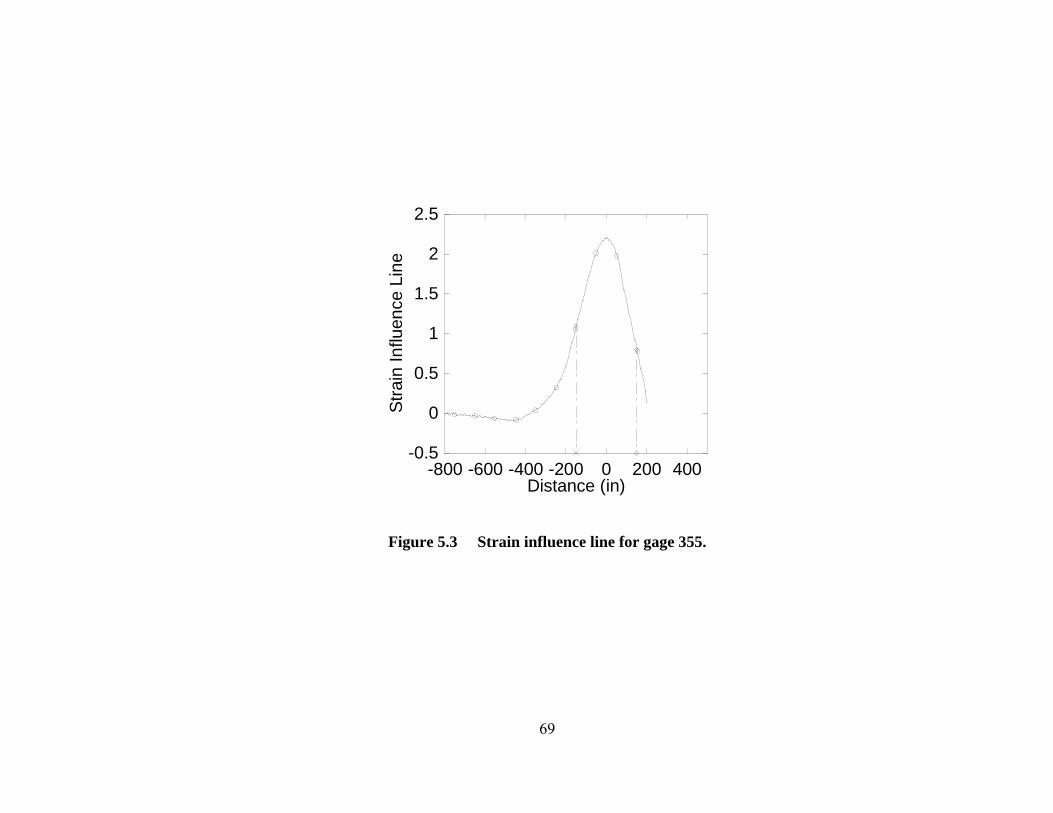
The cut-off on one side of the strain influence line plots for gages 346 and
355 (as shown in Figures 4.10d and 4.10e) is due to the fact that both gages are
attached to FB2. The strain influence line for FB2 obtained from strain gage 355 was
isolated in Fig. 5.3. The zero on the distance axis denotes the position of the floor
beam. On the right side is FB1 and FB3 is on the left side. Taking the strain value on
the plot at 150 inches on both sides of the floor beam (shown by the vertical straight
lines in Fig. 5.3), approximate values of 1.1 µε on the left side and 0.8 µε on the right
side were obtained. Since the bridge support is closer to the floor beam on the right
side, load on the right side causes less strain on the floor beam. Clearly, the beam
carries lesser load when the truck is on the side closer to the support than when it is on
the other side.
Thus, taking a mirror image of the continuous side of the floor beam (i.e.
not on the side of the support) result in a conservative strain influence line. By the
same reasoning, we can also predict that FB1, which is next to the bridge end, will
have lesser strain than the second floor beam under the same load.
-0.5
0
0.5
1
1.5
2
2.5
-800 -600 -400 -200 0 200 400
Stra
in In
fluen
ce L
ine
Distance (in)
Figure 5.3 Strain influence line for gage 355.
69
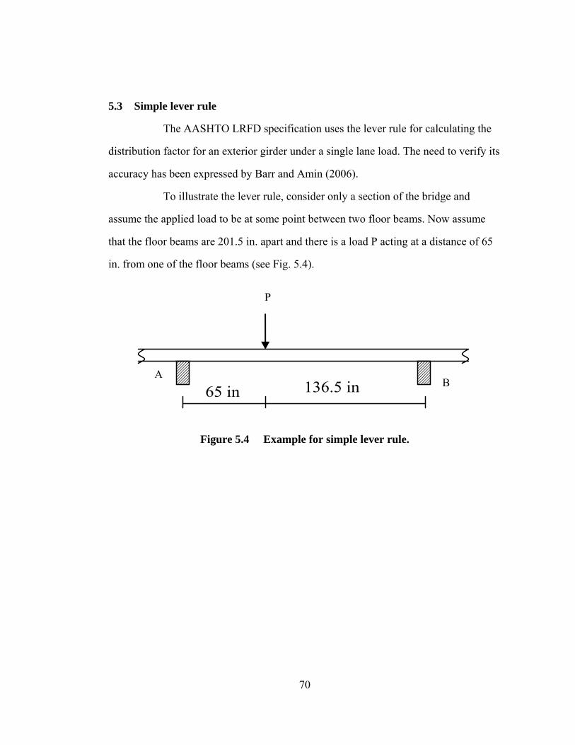
5.3 Simple lever rule
The AASHTO LRFD specification uses the lever rule for calculating the
distribution factor for an exterior girder under a single lane load. The need to verify its
accuracy has been expressed by Barr and Amin (2006).
To illustrate the lever rule, consider only a section of the bridge and
assume the applied load to be at some point between two floor beams. Now assume
that the floor beams are 201.5 in. apart and there is a load P acting at a distance of 65
in. from one of the floor beams (see Fig. 5.4).
P
136.5 in 65 in B
A
Figure 5.4 Example for simple lever rule.
70

Based on the lever rule, the load carried by floor beam A would be given
by
201.5136.5P
LyP ×=×
where, L is the total length between A and B, y is the distance of the load from B, and
the load carried by floor beam B would be
136.565.0P
LxP ×=×
where, x is the distance of the load from A. Thus, for a unit load, the load carried by floor beam A is equal to
0.677201.5136.5
=
and the load carried by floor beam B is equal to
0.323201.565.0
=
According to the lever rule, the entire load is said to be carried by the
floor beams only in the immediate proximity of the load and any other floor beams
further away are not considered to carry any part of the loads. If the load is exactly
above one of the floor beams, the entire load is assumed to be carried by that beam.
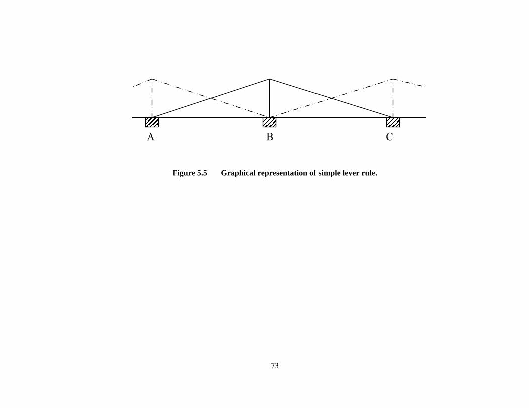
Fig. 5.5 provides a graphical representation of the lever rule. Here, the load is carried
fully by the intermediate beam B when the load is over B. The load carried by the
intermediate beam decreases as it goes further away from the beam. When the load
reaches the adjacent beam, it will be completely carried by that beam. The straight line
in Fig. 5.5 represents the lever rule for beam B and the dashed lines show the
application of the lever rule for beams A and C. The dashed lines becoming zero at B
shows that when the load is at position B, it has no effect on the beams A and C.
71

72
Similarly, the solid line becoming zero at A and C shows that beam B carries no load
when the load is at positions A or C.
73
A B C
Figure 5.5 Graphical representation of simple lever rule.
74
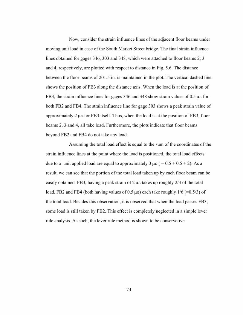
Now, consider the strain influence lines of the adjacent floor beams under
moving unit load in case of the South Market Street bridge. The final strain influence
lines obtained for gages 346, 303 and 348, which were attached to floor beams 2, 3
and 4, respectively, are plotted with respect to distance in Fig. 5.6. The distance
between the floor beams of 201.5 in. is maintained in the plot. The vertical dashed line
shows the position of FB3 along the distance axis. When the load is at the position of
FB3, the strain influence lines for gages 346 and 348 show strain values of 0.5 µε for
both FB2 and FB4. The strain influence line for gage 303 shows a peak strain value of
approximately 2 µε for FB3 itself. Thus, when the load is at the position of FB3, floor
beams 2, 3 and 4, all take load. Furthermore, the plots indicate that floor beams
beyond FB2 and FB4 do not take any load.
Assuming the total load effect is equal to the sum of the coordinates of the
strain influence lines at the point where the load is positioned, the total load effects
due to a unit applied load are equal to approximately 3 µε ( = 0.5 + 0.5 + 2). As a
result, we can see that the portion of the total load taken up by each floor beam can be
easily obtained. FB3, having a peak strain of 2 µε takes up roughly 2/3 of the total
load. FB2 and FB4 (both having values of 0.5 µε) each take roughly 1/6 (=0.5/3) of
the total load. Besides this observation, it is observed that when the load passes FB3,
some load is still taken by FB2. This effect is completely neglected in a simple lever
rule analysis. As such, the lever rule method is shown to be conservative.
Figure 5.6 Distance vs. strain influence line for three floor beams.
-0.5
0
0.5
1
1.5
2
2.5
-500 0 500 1000
346303348
Stra
in In
fluen
ce L
ine
Distance (in)
75
76
5.4 Application to load distribution
The previous analysis shows how the load is being distributed to the
individual floor beams with respect to the load position on the bridge. The trucks in
these cases were driven along the middle of the bridge. The response at the same
location when the load was a little further along the cross-section is desired. This will
take only two more passes (similar to Passes 6 and 8) but offset from the middle of the
roadway. In these new load cases, the tandem-axle truck was driven on the east side of
the bridge. These passes were labeled as Pass 11 and Pass 12. The transverse shift of
the truck path in these passes was approximately 2 ft., which was measured with
respect to the central longitudinal axis of the truck, towards the east side of the bridge.
The truck was driven backward in Pass 11 and forward in Pass 12 as shown in Table
4.2. The response recorded by each of the strain gages was recorded, and the data was
then processed as discussed in the Experimental Example in Chapter 4. The strain
influence lines for each strain gage location were obtained from Passes 11 and 12
(represented as East in Fig. 5.7) and then they were individually compared in Fig. 5.7
to the strain influence lines of the respective strain gages at center of the bridge
(shown as Final). The strain influence lines used for comparison are the final strain
influence lines obtained as the maximized average of the strain influence lines
obtained from the different sets of passes run through the middle of the bridge as
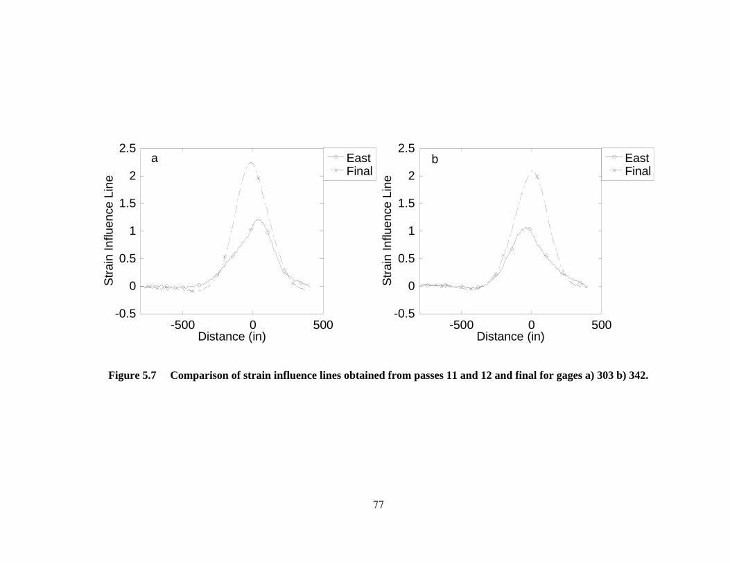
shown in Fig. 5.2.
-0.5
0
0.5
1
1.5
2
2.5
-500 0 500
EastFinal
Stra
in In
fluen
ce L
ine
Distance (in)
a
-0.5
0
0.5
1
1.5
2
2.5
-500 0 500
EastFinal
Stra
in In
fluen
ce L
ine
Distance (in)
b
Figure 5.7 Comparison of strain influence lines obtained from passes 11 and 12 and final for gages a) 303 b) 342.
77
-3
-2.5
-2
-1.5
-1
-0.5
0
0.5
-500 0 500
EastFinal
Stra
in In
fluen
ce L
ine
Distance (in)
c
-0.5
0
0.5
1
1.5
2
2.5
-500 0 500
EastFinal
Stra
in In
fluen
ce L
ine
Distance (in)
d
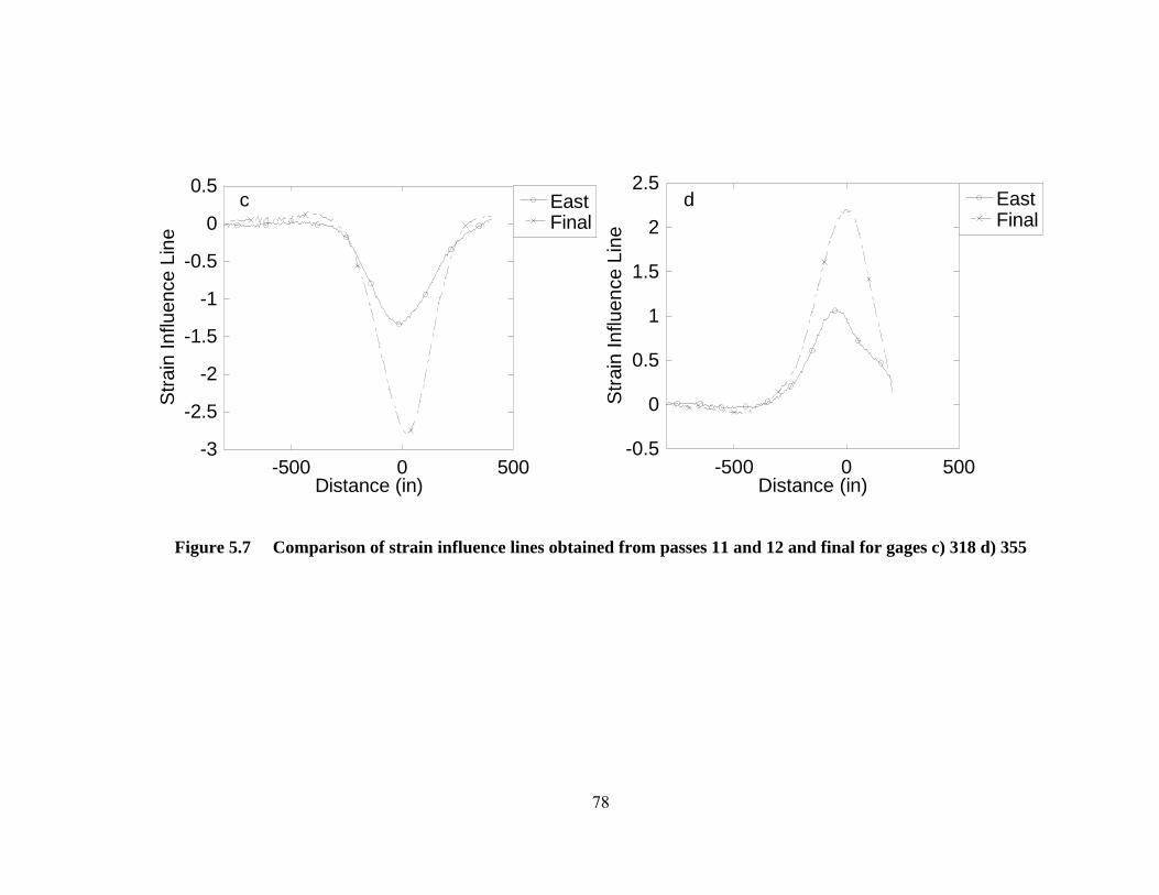
Figure 5.7 Comparison of strain influence lines obtained from passes 11 and 12 and final for gages c) 318 d) 355
78
-0.5
0
0.5
1
1.5
2
2.5
-500 0 500
EastFinal
Stra
in In
fluen
ce L
ine
Distance (in)
e
-0.5
0
0.5
1
1.5
2
2.5
-500 0 500
EastFinal
Stra
in In
fluen
ce L
ine
Distance (in)
f
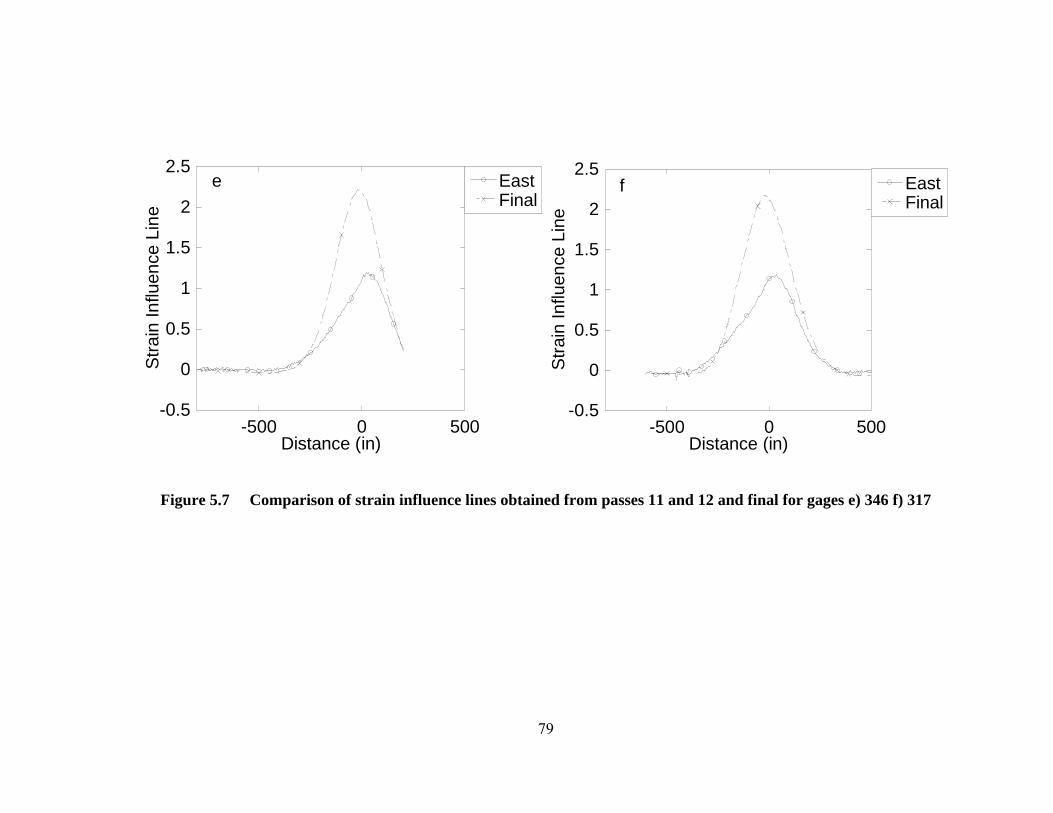
Figure 5.7 Comparison of strain influence lines obtained from passes 11 and 12 and final for gages e) 346 f) 317
79
-0.5
0
0.5
1
1.5
2
2.5
-500 0 500
EastFinal
Stra
in In
fluen
ce L
ine
Distance (in)
g
-3
-2.5
-2
-1.5
-1
-0.5
0
0.5
-500 0 500
EastFinal
Stra
in In
fluen
ce L
ine
Distance (in)
h
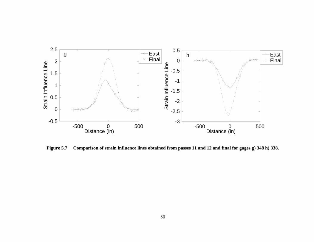
Figure 5.7 Comparison of strain influence lines obtained from passes 11 and 12 and final for gages g) 348 h) 338.
80
In all the plots in Fig. 5.7, the strain influence lines obtained from Passes
11 and 12 clearly have values less than those obtained from the Final strain influence
lines. Their peaks are approximately half of the peak of the Final strain influence
lines. The general shape is further confirmed by the resulting East strain influence
line. The symmetric property of the strain influence line, as seen in the Final strain
influence line, is not apparent in the East strain influence line (Fig. 5.7). The inability
to drive the truck in a straight line over the bridge, and also the difficulty in
maintaining a constant offset of 2 ft. from the bridge centerline might account for this
asymmetry in the East strain influence line. However, it is clear that just a slight offset
of 2 ft. in the approximately 20 ft. wide bridge (excluding overhangs) causes a
significant strain decrease at the mid-span of the floor beam. The load being moved
towards the supporting girder has less of an effect on the floor beam. This observation
shows that the load effect along the cross-section could be significant. Therefore,
strain gages should be put linearly along the cross-section, including at the girders, to
learn more about the load distribution.
5.5 Sensitivity study
To get the strain influence lines, the axle weights were multiplied by a
certain factor to equalize one of the axle weights of the trucks. Through subtraction,
the strain due to a point load with the magnitude of the difference of the remaining
axle weight was obtained. If both axle weights were initially equal, upon factoring,
there will be no point load after subtraction. In such a case, the strain influence line
would not be obtained. Thus, to get an influence line, a different ratio of the front axle
weight to rear axle weight of the two trucks is required. The method of running a truck
forwards and then backwards has been shown to work as seen by Passes 6 and 8. If the
81

82
front to rear axle weights ratio of the truck is r when it moves forwards, the ratio of
the front to rear axle weights of the truck is 1/r when it moves backwards. Unless r is
equal to 1, there will be a different ratio of the front to rear axle weights. Therefore,
moving the truck in both directions should give the strain influence line.
As mentioned earlier in Test Results, Passes 13 and 14 had a lot of noise
in the measurements. These were the passes carried out with the empty tandem-axle
truck. Using a loaded truck once and the empty truck the second time gave us different
axle loads maintaining the requirement of same axle spacing. The front axle weight
did not change as much as the rear axle weight due to the truck configuration. The raw
data (strain vs. time) of Pass 14 is compared to that of Pass 6 in Fig. 5.8. No
significant difference can be seen in the raw data.
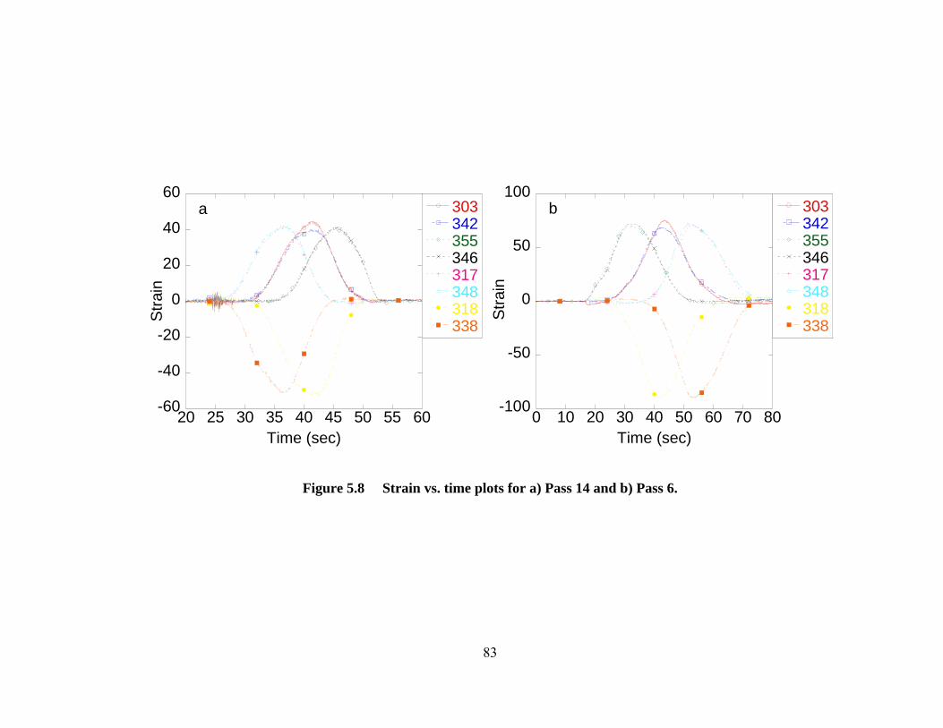
-60
-40
-20
0
20
40
60
20 25 30 35 40 45 50 55 60
303342355346317348318338S
train
Time (sec)
a
-100
-50
0
50
100
0 10 20 30 40 50 60 70 80
303342355346317348318338
Stra
in
Time (sec)
b
Figure 5.8 Strain vs. time plots for a) Pass 14 and b) Pass 6.
83
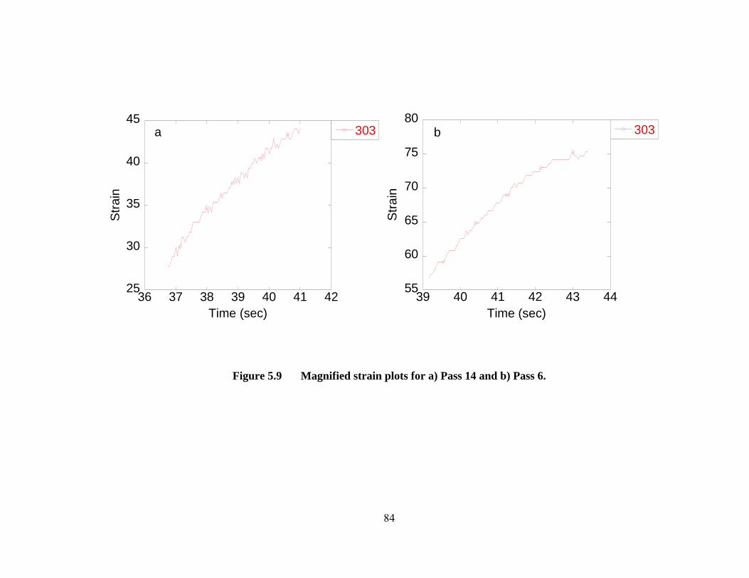
25
30
35
40
45
36 37 38 39 40 41 42
303St
rain
Time (sec)
a
55
60
65
70
75
80
39 40 41 42 43 44
303
Stra
in
Time (sec)
b
Figure 5.9 Magnified strain plots for a) Pass 14 and b) Pass 6.
84

85
The strain was recorded at a rate of 20 Hz. The strain plots are blown up
for a portion of the raw data and a lot of noise can be seen in the strain plots. This
could be due to the empty truck which may vibrate more while running over the
bridge. After going through the usual manipulations and processes, the final strain
influence line was derived by pairing up Pass 14 with Pass 3. The same truck, but
loaded, was used in Pass 3. The strain influence line obtained is shown in Fig. 5.10a.
Clearly, the data obtained from Pass 14 is problematic. Thus, we recommend that only
heavily loaded trucks be used.
Figure 5.10 Strain influence lines obtained from Pass 3 and Pass 14.
-3
-2
-1
0
1
2
3
200 400 600 800 1000 1200
303342355317346348318338
Stra
in In
fluen
ce L
ine
Distance (in)
a
86

Chapter 6
CONCLUSION
With the continued deterioration of the nation’s bridges, combined with
limited financial resources for maintenance and reconstruction, comes the need for
tools to enable effective bridge management decisions. Accurate bridge condition
information is critical in making bridge management decisions. One increasingly used
tool for determining accurate bridge condition assessments is field load tests. Over the
past decade, improved techniques and technologies have enabled more and more states
to utilize field tests as part of the bridge management program. The most commonly
used testing method is called diagnostic testing.
In this thesis, an experimental influence line test procedure is developed
and demonstrated. The procedure is similar to, although simpler than, diagnostic load
tests. In addition, the method makes use of the powerful concept of influence lines.
Influence line are excellent for bridge evaluation because they give engineers insight
into a bridge’s load distribution due to moving loads (i.e. trucks), and hence provide a
direct way of determining a bridge’s load carrying capacity under different load
configurations. The results of experimental influence line tests can therefore be very
helpful in the assessment of load distribution, the determination of overall bridge
condition, and the ability of a bridge to carry overweight permit vehicles.
The experimental influence line test procedure developed uses trucks of
known weight and axle configurations. While experimental influence lines for long
span bridges are easy to obtain, a suitable test design is needed for short to medium
87

span bridges. In the procedure, strain gages were attached to the members for which
influence lines are to be generated. During the tests conducted, both two-axle trucks
and tandem-axle trucks having known axle weights and axle spacings were driven
across a bridge in specific patterns. These patterns were referred to as the forward-
backward method, stopping method, the empty truck method, and the northbound-
southbound method. Procedures were then developed and demonstrated for reducing
the raw experimental data collected, which represents influence profiles, into
influence lines due to a unit load.
It has been shown that an experimental influence line test can be
performed on a bridge using minimal instrumentation and by using available service
trucks. The viability of using both two-axle and tandem-axle trucks was investigated.
In situations where two-axle trucks are not available, tandem-axle trucks, which are
more common, can be used. It has been shown that empty (i.e. very light) trucks are
undesirable due to the vibrations they produce on the bridge and the resulting noise in
the experimental strain data.
Based on the field test performed, the experimental strain influence lines
obtained for the South Market Street bridge were found to be consistent for all strain
gage locations. All floor beams tested had identical section properties, and all yielded
very similar strain influence lines (i.e. similar peak value and shape of curve). The
strain influence lines for an intermediate floor beam were shown to be different than
those of the end floor beams. The strain influence lines from different load methods
were shown to be quite comparable. Of the various methods tested, the biggest
difference is that the stopping method involves much less data manipulation after the
test, but takes slightly longer to conduct in the field.
88
After analyzing the test results, it was determined that the simple lever
rule overestimated the load effects on the bridge. It was found that no more than two-
thirds of any axle load is carried by a single floor beam, and the remaining portion of
the axle load is carried by the adjacent floor beams. Based on the lever rule, 100% of
an axle load is assumed to be carried by the floor beam when the axle is directly over
the floor beam. The actual amount of load carried by the floor beam may differ in
different bridges depending on the spacing of the floor beams, structural framing
details, and deck types and configurations.
With regards to load distribution as a function transverse truck location on
the bridge deck, it was found that when the truck was shifted only 2 feet away from
the mid-span of the floor beam, it produced approximately half of the strain at the
mid-span compared to when the truck was centered on the deck.
The work performed has developed a very practical and useful testing
methodology. It is recommended that additional studies be conducted to further refine
the method, and to study specific bridge performance parameters. Some suggestions
include a more detailed study of the effects of transverse load distribution due to truck
passes in the same direction but along different longitudinal axes on the bridge. It is
also recommended that future studies include strain gages placed along the length of
the floor beams to acquire additional data on transverse load distribution. Girders
might also be instrumented to get the load effects on them (especially in case of
multiple girders). Finally, it is recommended that tests on bridges, having different
floor beam spacings, geometries, and deck types be conducted in order to draw more
general conclusions regarding load distribution rules for bridge floor beams.
89

BIBLIOGRAPHY
Barr, P. J. and Amin, MD. N. “Shear live-load distribution factors for I-girder bridges.” Journal of Bridge Engineering, ASCE, 2006, 11(2), 197-204.
Akgül, F. and Frangopol, D. M. “Bridge rating and reliability correlation: Comprehensive study for different bridge types.” Journal of Structural Engineering, ASCE, 2004, 130(7), 1063-1074.
Chajes, M. J., Shenton III, H. W., O’Shea, D. and Chaudhari, M. “Using bridge testing to enhance bridge management in Delaware.” Proceedings of the 9th International Bridge Management Conference, TRB, 2003, Orlando, Florida.
Catbas, F. N. and Aktan, A. E. “Condition and damage assessment: issues and some promising indices.” Journal of Structural Engineering, ASCE, 2002, 128(8), 1026-1036.
Malek, A. and Jáuregui, D. V. “Computer-aided graphical analysis of bridges under vehicular loading.” Journal of Bridge Engineering, ASCE, 2001, 6(3), 207-212.
Chajes, M. J., Shenton III, H. W. and O’Shea, D. “Bridge condition assessment and load rating using nondestructive evaluation methods.” Journal of the Transportation Research Record, TRB, 2000, 1696(2), 83-91.
Zokaie, T. “AASHTO-LRFD live load distribution specifications.” Journal of Bridge Engineering, ASCE, 2000, 5(1), 131-138.
Sartor, R. R., Culmo, M. P. and DeWolf, J. T. “Short-term monitoring of bridge structures.” Journal of Bridge Engineering, ASCE, 1999, 4(3), 157-164.
Chajes, M. J., Mertz, D. R. and Commander, B. “Experimental load rating of a posted girder-and-slab bridge.” Journal of Bridge Engineering, ASCE, 1997, 2(1), 1-10.
Buckley, E. “Basic influence line equations for continuous beams and rigid frames.” Journal of Structural Engineering, ASCE, 1997, 123(10), 1416-1420.
90

Alampalli, S. and Fu, G. “Influence line tests of isotropically reinforced bridge deck slabs.” Client Report 54, Engineering Research and Development Bureau, 1992.
91