Reprinted from International Journal of Flow Control

Reprinted from

International Journal of Flow Control

Volume 3 · Number 1 · March 2011

Multi-Science Publishing

ISSN 1756-8250

An Experimental and Modeling

Investigation of Synthetic Jets in a

Coflow Wake

by

Xi Xia and Kamran Mohseni

An Experimental and Modeling

Investigation of Synthetic Jets in a

Coflow Wake

Xi Xia1’* and Kamran Mohseni1’2†

1 Department of Mechanical and Aerospace Engineering,2 Department of Electrical and Computer Engineering,

University of Florida, Gainesville, FL 32611

Abstract

A round synthetic jet injected in a coflow wake is investigated experimentally in order toestimate the spreading and decaying rates of the jet while compensating for the actuatorwake. The flow field of the jet and wake is measured using hot-wire anemometry. Thespatial evolution of the synthetic jet is modeled similarly to a continuous turbulent jet ina coflow with some modifications for the pulsatile nature of the synthetic jet and thewake behind the flow actuator. The model employs an integral formulation thatconserves the excess momentum flux in the jet along with a hypothesis which asserts thatthe rate of growth of the shear layer is proportional to the velocity of the dominant eddiesin the jet relative to the surroundings. The characteristic velocity and length scales arederived from a corresponding top hat velocity profile. The jet in the far field is observedto exhibit self-similar behavior, as distinguished by the overlapping of the excess meanvelocity profiles if scaled by the self-similar variables. The streamwise variation of thecenterline velocity shows good agreement with the proposed semi-empirical integralmodel. The verification of the theoretical model suggests that the decay of the non-dimensional relative velocity of the jet depends mostly on the spreading rate of the samesynthetic jet in a quiescent environment. The spreading rate of the synthetic jet decreasesas the coflow velocity increases. Finally, for a synthetic jet in a coflow wake, a largeractuator stroke ratio results in a faster velocity decay as well as an enhanced spreadingrate.

Nomenclature

bg half width of jet for a Gaussian velocity profileB half width of jet for a top-hat velocity profiled diameter of orificef frequency of oscillationH height of cavityh depth of orificeKe excess kinematic momentum fluxβg jet spreading rate for gaussion profileβ jet spreading rate for top-hat profileL length of slugL/d stroke ratioRe reynolds numberr radial coordinateT time period of oscillationUj mean jet exit velocityu streamwise jet velocityUa local effective coflow velocity (uniform coflow velocity)

Volume 3 · Number 1 · 2011

19

*Graduate Student, Department of Mechanical and Aerospace Engineering.†W. P. Bushnell Endowed Professor, Department of Mechanical and Aerospace Engineering and Department of Electrical and Computer

Engineering, Associate Fellow of the AIAA.

Uc centerline jet velocity for a free synthetic jetUt wind tunnel velocityue velocity in excess of the coflow velocity∆Ug centerline excess velocity∆U jet excess velocity for top-hat profileVd driving voltagex axial coordinatexo virtual originl* excess momentum length scaleU* scaled excess velocity for top-hat profileB* scaled half width of jet for top-hat profilex* scaled streamwise distanceν kinematic viscosity of fluid

A synthetic jet is a zero net mass flux (ZNMF) and fully pulsatile jet that results from the formation andinteraction of vortex rings or pairs [1]. A common method of generating a synthetic jet is to apply a periodicpressure gradient across the orifice of a cavity. This affects the cyclic inception of a shear layer at the orificeedge, which in turn, rolls up into a vortex ring that travels downstream due to its induced velocity. Figure1 shows a schematic of the suction and ejection strokes that constitute cycles in this synthesis. In thisfashion, a train of vortex rings moves away from the orifice, whereupon they interact, and break down ina transition towards a turbulent jet directed downstream. This operational principle allows for a synthetic

20 An Experimental and Modeling Investigation of Synthetic Jets in a Coflow Wake


noitcejE)b(noitcuS)a(

Figure 1: Schematic of synthetic jet operation displaying the suction and ejection strokes. (a) Suction; (b)Ejection.

jet to be synthesized entirely from the surrounding medium, while at the same time imparting a netmomentum flux to the surrounding environment. In addition, the ability to influence the surroundingmedium at a variety of scales has made synthetic jets attractive for a number of applications [2].

Flow control is the major area of application for synthetic jets; for example, some synthetic jetactuators have been designed to reduce drag by introducing disturbances into the boundary layeradjacent to a flow structure, thereby enhancing momentum transfer within the shear layer andforestalling separation [3, 4]. Similar concepts have been employed in underwater vehicle propulsionand low speed maneuvering [5, 6]. Micro synthetic jets have also been proposed for propulsion of tinyendoscopy capsules inside the human body [7, 8]. Finally, synthetic jets have been shown to modify theaerodynamic characteristics of airfoil surfaces [9, 10] and enhance aerodynamic lift of fixed wing microair vehicles in wind tunnel tests [11].

Synthetic Jets in Coflow. In order to design synthetic jet actuators for these applications, a model ofthe evolution of the emerging jet is required. In practice, the surrounding medium is rarely stationaryand may possess parallel, perpendicular or swirl velocity components. While most semi-empirical andnumerical models of the mean velocity fields focus on jets injected into a quiescent environment [1, 12,13, 14], less focus has been directed towards coflow or crossflow configurations [15, 16]. Consideringthat the characteristics of a jet changes if an external flow is present, this study is focused on extendinga semi-empirical modeling technique for continuous jets to synthetic jets operating in a coflow

downstream of the actuator wake.Figure 2 shows a schematic of a synthetic jet in an ideal coflow. The near field of the synthetic jet is

typified by the presence of discrete coherent vortex rings and fully pulsatile flow. The effect of coflow onthe formation of vortex rings, has been investigated and shown to reduce the strength of vorticity of thestarting vortex rings and to delay the vortex pinch-off process [17]. Further downstream, the flow spreadsfurther away from the orifice and breaks into a turbulent jet with many similarities to a turbulent continuousjet.

Synthetic jets in a quiescent environment share many features of their continuous jet counterparts.These include experimental self-similarity of the flow as inferred from the overlapping of the scaledmean and turbulent intensity profiles [1, 18]. In this investigation we will show that many of thesesimilarities may be extended to the case of synthetic jets in coflow wakes. In the far field, the effect ofthe coflow on a continious turbulent jet is shown to enhance the advection of the jet, while reducing thejet spreading rate [19, 20, 21]. The counterpart of this region for a synthetic jet is the focus of this study.

The Proposed Modeling Technique. As synthetic jets exhibit several similarities to continuous jets[1, 2], here we develop a model for a synthetic jet in a coflow by modifying a similar model forcontinuous jets. Modeling a jet in a coflow involves predicting the velocity decay and spreading of thejet as it interacts with the background flow. Most models of continuous jets in a coflow assume that theflow is self-similar at some distance from the jet origin. This reduces the problem to one of solving forthe streamwise variation of an appropriately chosen characteristic length and velocity scales in the jet.Two relevant equations are then required to determine these two unknowns. For the first equation, usingan integral formulation, most models have assumed that the streamwise excess momentum flux isconserved, resulting in a relationship between the length and velocity scales. One additional equationis then required to determine the streamwise variation of the velocity and length scales. This is whereseveral approaches have been proposed in the literature on continuous jets. One method employs asecondary momentum integral in conjunction with the Prandtl mixing length theory while assuming aconstant eddy viscosity throughout the flow [22]. Despite the results being comparable to experimentaldata, the streamwise variation is not predicted correctly. This is attributed to the inaccurate of theconstant eddy viscosity hypothesis. Another approach employs higher order moments of themomentum equation without using any phenomenological assumptions [23]. This model did not showgood experimental agreement for weak jets or the far field of strong jets where the excess velocity wascomparable to the coflow velocity. Another method applies a double integral method while employinga large eddy hypothesis, which essentially relates the Reynolds stresses to the shear strain rate throughthe length scales of the largest eddies in the shear flow [24]. Again, this model does not agree well withthe experimental data. An alternative approach is to use an equation to relate the growth of the shearlayer, and consequently the length scale, to the velocity scale in the flow based on the jet entrainment[25, 26]. It is found that this approach results in accurate predictions for weak jets only. In summary,these techniques for continuous jets all show poor performance at least in some flow regions and failto offer a good agreement with experimental data over the entire range of the jet and coflow field

Xi Xia and Kamran Mohseni 21


Figure 2: Schematic of the evolution of a round synthetic jet in a coflow, showing a vortex ring in the nearfield, and mean velocity profiles of the jet in the far field.

strengths. Recently, a model employing the conservation of excess momentum and an auxiliaryequation for a spreading hypothesis has shown much better agreement with experimental data [21]. Thekey difference among these techniques lies in the selection of the characteristic length and velocityscales. The previous models derive the characteristic length and velocity scales directly from anassumed Gaussian-like mean velocity profile while an equivalent top hat velocity profile is defined andemployed in [21]. Moreover, this new model agrees well with experimental data over a wide range ofcontinuous jet strength. We will extend similar ideas to synthetic jets in a coflow wake here.

As mentioned previously, we have already developed a model for a synthetic jet in quiescentenvironment. Our model accounts for the enhanced spreading and decaying rates of a synthetic jet, causedby the pulsatile nature of the flow, through an enhanced eddy viscosity value1. This eddy viscosity isdirectly related to the momentum of the jet which is dictated by the actuator and its operating parameters.On the other hand, for modeling a synthetic jet in a background coflow, one requires to provideinformation about the coflow parameters as well. Furthermore, since actual synthetic jets have a finitedimension, a wake is expected downstream of the actuator. Information about the actuator wake is alsoexpected to influence the result. Therefore, in this investigation, a model for synthetic jets in coflow, andmore generally, in coflow wakes is proposed where the effect of the coflow on the jet is modeled whilethe impact of the actuator wake is properly addressed. This model was inspired by models of continuousjets in coflow which have been used to predict the mean behaviors of the jet and to identify the dominantparameters controlling the jet spreading and decay. These parameters are the coflow velocity and the jetmomentum. Similar to extending the model of free continuous jets to synthetic jets, the validity ofextending this model from continuous jets in a coflow to synthetic jets in a coflow requires the use of anenhanced eddy viscosity to account for the enhanced mixing and spreading rates of a synthetic jet. We alsoassume that the excess mean velocity profiles of a synthetic jet in coflow display self-similarity in the farfield. This assumption is experimentally validated posteriori. After the model is established, experimentsare conducted to study the jet flow field using a hot-wire anemometry. While a continuous coflow jetcould be easily formed by placing the exit of a pipe connected to a pressurized fluid tank in a backgroundflow, a synthetic jet is synthesized from the surrounding fluid itself. As a result, the entire jet actuator isrequired to be placed in the background flow. This introduces a new modeling challenge as the wakebehind a synthetic jet actuator is significantly larger than a corresponding continuous jet setup, andtherefore, additional compensations need to be made to resolve the coflow wakes instead of a uniformcoflow.

This manuscript is organized as follows. Section 1 briefly outlines the self-similar model for acontinuous jet in a coflow and addresses the changes that need to be made to account for using asynthetic jet in a coflow wake background. The experimental setup for the measurement of the velocityfield is then described in Section 2. The results are presented and discussed in Section 3. Concludingremarks are summarized in Section 4.

1. THEORETICAL MODEL

In this section, we first review the theoretical framework for modeling a continuous jet in a uniformcoflow [21]. We will then extend the model to the case of a synthetic jet in a coflow with significantactuator wake effects.

1.1. Continuous Jets in a Coflow

Figure 3 shows a schematic of the mean velocity profile in the far field of a turbulent jet formed froma round orifice of diameter d injected parallel to a free stream with a uniform velocity Ua. For modelingpurposes, the far field of the jet in a coflow may be modeled as if it were generated by a continuouspoint source of momentum in a flow parallel to the jet. The velocity in excess of the coflow velocity atany position is then given by

(1)

where x indicates the streamwise direction and r is the radial direction.The excess velocity profile in the far field of a continuous turbulent jet is known to exhibit a self-

u x r u x r Ue a( , ) ( , ) .= −



1This observation and the measurement and modeling of the enhanced eddy viscosity of a syntheticjet has been the focus of several publications from our group [13, 14, 27]

similar behavior [19, 20] and to be well approximated by a Gaussian profile given by

(2)

where ∆Ug is the centerline excess velocity and bg is the characteristic width of the jet, defined as theradial distance where ue � ∆Ug. Using boundary layer approximations, it can be shown that theexcess kinematic momentum flux, Ke, defined as

(3)

is conserved in the streamwise direction for a continuous jet in a coflow [28]. As the behavior of the jetis dependent primarily on Ke and Ua, an excess momentum length scale may be defined by

(4)

In this study, we make the assumption that the width and the mean strength of the excess velocityprofile are the most relevant parameters for modeling a jet in a coflow. While a Gaussian velocityprofile approximates well the real excess velocity distribution in the far field of a continuous jet, itcarries more information than needed for our modeling purposes. To avoid unnecessary complications,in this study we limit ourselves to a top-hat excess velocity profile with only two main characteristicscales; namely, the width B and the amplitude ∆U. As seen shortly, this implies that the changes in thevelocity profile may be rather simply characterized by two parameters of an equivalent top hat velocityprofile (shown in Figure 3) that can be described as:

The use of this top hat profile can be motivated by the need to identify proper velocity and width scalesfor the jet so that the spreading and decaying behaviors are modeled straightforwardly. Therefore, thesecharacteristic scales are determined from a conservation prospective of the excess mass flux and excessmomentum flux so that the large scale eddies with a length scale on the order of B are responsible for

uU r B

r Be =<>

∆0

lK

Ue

a

* = ⋅

K uu rdre e=∞

∫20

π ,

1e

u

Uee

g

r

bg

∆=

−2

2

,



Figure 3: Schematic of the mean Gaussian and equivalent top-hat velocity profiles in a continuous jet in auniform background flow.

jet spreading and they are advected with respect to the ambient coflow at a velocity of ∆U. Therelationship between the top-hat and Gaussian profiles could be derived by equating their excess massand excess momentum fluxes. These conditions are given by:

(5)

and

(6)

Solving the above equations for the velocity profile given in Eq. 2, yields

(7)

and

(8)

To relate the jet width to the jet velocity, it is assumed that the change in the width of the shear layermoving with the eddies is proportional to the relative velocity between the jet and the surroundings.That is

(9)

where β is the proportionality factor and the characteristic velocity and length scales are obtained fromthe top hat velocity profile. Assuming that β remains constant for a given jet, the above relation shouldhold for a continuous jet in a quiescent environment in which case Ua � 0. Here, the spreading rate forthis free continuous jet is designated as βg, which is calculated from the characteristic jet width bg.Therefore

(10)

The conservation of excess momentum flux defined in Eq. 3 for the top hat velocity profile yields

(11)

which, using Eq. 4, can be rearranged to

(12)

The excess momentum Eq. 12 and the spreading hypothesis in Eq. 9 can be nondimensionalized to

(13)

and

(14)dB

dx

U

Ug

*

*

*

* ,=+

21

β

U UB

* ** ,22

10+ − =

π

∆ ∆U

U

U

U

l

Ba a

+

−

=2 2

2 0*

.π

K B U U B U U Ue a= = +( )π π2 2∆ ∆ ∆ ,

β β= ⋅2 g

dB

dtU U

dB

dxUa= + =∆ ∆β ,

B bg= ⋅2

∆∆

UUg=2

,

π πB U U U uu rdra e2

02∆ ∆+( ) =

∞

∫ ,

π πB U u rdre2

02∆ =

∞

∫ ,



where U* � ∆U/Ua, B* � B/l*, and x* � x/l*. The initial conditions for this set of equations can be

written as U*o � ∆Uo/Ua and Bo

* � Bo/l* where Uo and Bo are the measured values at some convenientpoint in the turbulent far field region. Equations 13 and 14 are coupled differential equations whichpredict the streamwise evolution of the velocity magnitude and its spreading. This approach has beensuccessfully employed in modeling continuous jets in a coflow [21].

1.2. Extending Continuous Jet Model to Synthetic Jets in a Quiescent Environment

The previous discussion demonstrates the need for a model that extends the continuous jet theory tosynthetic jets. Actually, as will be discussed in the following section, there is a far field region for asynthetic jet that displays the same self-similarity that is seen in turbulent continuous jets. This providesthe basis for the possibility of finding a self-similar solution for a synthetic jet in a similar approach asthat for a continuous jet.

One classic self-similar solution for free continuous jets is the Schlichting [29] solution. The far fieldof a continuous jet may be thought of as being generated by a continuous point source of momentum inan infinite incompressible fluid. It is admissible to describe the mean velocities in the continuous jet byboundary layer equations. For a self-similar solution to the boundary layer equations to exist, thestreamwise pressure gradient must be zero, whereupon a closed form solution for a laminar jet may befound [29]. It was later seen [30] that the turbulent jet could be modeled using the same differentialequations that described the laminar jet, but with the laminar viscosity coefficient replaced by an effectiveeddy viscosity coefficient associated with the turbulent jet. Following along these lines it is hypothesizedhere that the mean velocity field of a synthetic jet may be modeled as a laminar free jet, so long as oneuses an effective viscosity coefficient obtained empirically instead of the usual viscosity. Next, a roundcontinuous jet model will be introduced and then the compatibility with a synthetic jet will be discussed.

In cylindrical coordinates the boundary layer equations with no pressure gradient are written as

(15)

where u and υ are the streamwise and radial velocity components respectively, τ is the total shear stress,and ρ is the fluid density. The total shear stress may be related to the mean velocity using an eddyviscosity approximation

(16)

where, v is the laminar kinematic viscosity, ετ is the turbulent eddy viscosity coefficient, and ε is thetotal or effective eddy viscosity that takes into account both the laminar and turbulent contributions tothe shear stress. While the eddy viscosity hypothesis assumes that momentum transfer in a turbulentflow is dominated by large scale eddies, it also characterizes the mixing due to turbulent fluctuations,which in turn determine the rate of spreading of a free jet.

The eddy viscosity may be derived from the experimental data as follows: Assuming that theevolution of the jet is dependent only on local length and velocity scales and lacks memory of theorifice dimensions itself, the streamwise mean velocity profiles may be considered self-similar. Fromthe conservation of streamwise momentum it may be shown that the characteristic length (b) andvelocity (u) of the jet scale as x and x�1 respectively. The self-similar assumption then leads to astreamwise velocity profile of the form The similarity variable written as, isrelated to the effective viscosity coefficient through a free constant σ. Since the mixing lengthhypothesis assumes that the effective viscosity is constant over the entire jet, the boundary layerequations may then be reduced to an ordinary differential equation of the form ff� � f� — η f�. Fromthe conservation of momentum and the assumed form of the velocity distribution the streamwisevelocity is solved to be

(17)uK

x=

+( )3

8

1

1 14

2 2πε η,

η σ= rx ,u x f r

x= ( )−1 .

τ ρ ε ρετ= +( ) ∂∂

= ∂∂

vu

r

u

r,

∂∂

+ ∂∂

+ = ∂∂

+ ∂∂

=∂( )

∂u

x r ru

u

x

u

r r

r

r

υ υ υρ

τ0

1, ,and



with the self similarity variable given as

(18)

K, the kinematic momentum of the jet, is a measure of the strength of the jet and is obtained as

It is important to note here that the above analysis assumes a constant momentum fluxin the streamwise direction. While this is applicable to continuous jets, in synthetic jets it has beenreported that the momentum flux at the orifice is higher than that in the far field [1, 31]. The momentumflux was shown to decrease in the near field of the jet due to an adverse pressure gradient, and thenasymptote in the far field to some fraction of the exit momentum flux. It is this reduced asymptotic valueof the momentum flux that should serve as the magnitude of the driving momentum flux in the abovesimilarity analysis for the synthetic jet, and not the exit momentum flux at the orifice of the actuator.

The eddy viscosity, ε is now obtained from the spreading and decay rates of the jet. At the centerlinethe streamwise velocity may be expressed as

(19)

where Su is a measure of the jet decay rate. The radial extent of the jet at a particular axial station maybe characterized by a half width (b1/2), defined as the radial distance from the centerline at which thestreamwise velocity drops to half the centerline velocity. The linear streamwise variation of the halfwidth may be written as

(20)

where Sb is the spreading rate of the jet. From Eq. 17 through 20 the free constant σ in the similarityvariable is related to the spreading rate as

(21)

from which the eddy viscosity is related to the spreading rate and decay rate as

(22)

In summary, Equation 17 and 22 give the self-similar solution that could be applied to the far field ofa turbulent jet: either continuous jet or synthetic jet. Thus, in this study, we are trying employ the sametechnique as above to extend continuous jet coflow model to synthetic jet.

1.3. Synthetic Jets in a Coflow Wake

As mentioned earlier, similarities between synthetic and continuous turbulent jets motivate extendingthe model developed in the previous section to synthetic jets. However, three particular differencesneed to be taken into account before that theory could be applied to synthetic jets in coflow wakes. Thefirst is the increased spreading rate of a synthetic jet in comparison with a counterpart continuousturbulent jet. While a nominal spreading rate for a continuous turbulent jet is about 0.11 [30, 32], thevalue for a synthetic jet may vary greatly depending on the forcing conditions and upon a non-dimensional operational parameter called the stroke ratio (L/d) [1, 13, 33, 34]. The stroke ratio is theratio of the length of the slug of fluid ejected from the orifice during the expulsion stroke to thediameter of the orifice. It may be obtained through the criteria that the volume displaced by themembrane inside the actuator cavity is equal to the volume ejected from the orifice.

The pulsatile nature of synthetic jets allows for the definition of the characteristic velocity scale tobe defined based on either ejected volume or momentum flux of the jet [33, 13]. It is more appropriate

ε =−( )

1

8 2 1

2S

Sb

u

.

σ = −2 2 1

Sb

,

b S xb1 2/ ,=

uK

x S xcu

= =3

8

1

πε,

K u rdr=∞

∫2 2

0π .

ηπ ε

= 1

4

3 K r

x,



to use the velocity scale based on momentum flux in this study, as the self-similar jet solutions defineequivalent jets based on momentum flux rather than mass flux. Thus the velocity scale is given as

where the associated Reynolds number is defined by

(23)

The enhanced spreading rate of a synthetic free jet may be attributed to the enhanced mixing andentrainment of the ambient flow brought about by the periodic introduction, advection, and subsequentinteraction of vortical structures [13, 14]. Krishnan and Mohseni [13, 14] showed that the enhancedspreading rate of a synthetic jet could be accounted for by an enhanced eddy viscosity coefficient. Theywere able to use the jet self-similarity to measure the eddy viscosity coefficient for synthetic jets. Toextend the coflow model of section 1.1 to synthetic jets, the spreading rate of a continuous jet (β) mustbe replaced by that of a synthetic jet in a quiescent environment so that this enhanced spreading ratemay be taken into account in the coflow configuration. Systematic measurement of the spreading rateof synthetic free jets are conducted in [13, 14].

The second difference between synthetic and continuous jets which needs to be accounted for liesin the conserved momentum flux assumption in the self-similarity analysis of a jet in a quiescentenvironment. This translates into the conservation of excess momentum flux in a coflow configuration.This conservation assumption is derived by assuming that there is no pressure gradient in thestreamwise direction. While this is more readily applicable to continuous jets, it is not always accuratefor synthetic jets. It has been observed that as a result of a pressure gradient near the orifice of thesynthetic jet, the momentum flux could decrease in the streamwise direction, reducing to someasymptotic value in the far field [1, 31]. Thus, the above self-similar analysis is applicable after theexcess momentum flux reaches a constant value. In this study, the excess momentum flux in equation3 is obtained from the measured velocity profile downstream of the orifice.

Finally, the theory developed in the previous section assumes that the footprint of the continuous jetactuator is rather small and of the same order of magnitude as the diameter of the pipe issuing the jet. In thiscase, the wake of the actuator is quite negligible, with minimal effect on the background uniform coflowvelocity. This assumption is not really accurate for synthetic jets in a coflow where the entire actuator isrequired to be placed in the coflow. As a result, the size of the wake behind the synthetic jet actuator scaleswith the size of the actuator itself instead of the size of the originating jet, i.e., that is the orifice diameter. Asa result, the coflow velocity for a synthetic jet can not be treated as a uniform background flow and the effectof the actuator wake needs to be properly accounted for in order to derive a more accurate model.

In this study, the coflow velocities vary in both spanwise and streamwise directions inside the wakeregion. As discussed in the previous section, the coflow velocity Ua is an important parameter affectingthe characteristic length and velocity scales. Therefore, it is natural to define the characteristic coflowvelocities for the wake with respect to the wake velocity at different streamwise locations from theactuator. To simplify the characterization of the wake velocity field, the top-hat profile is adopted hereand the wake velocity profiles are then averaged while maintaining momentum balance, as shown inFigure 4. The local equivalent coflow velocities for the wake region can then be represented by

(24)

where uw is the actuator wake velocity profile measured without the synthetic jet actuator beingactuated. It should be noticed that the choice of the integration region for the wake is the same as thejet top-hat width because this region is where the synthetic jet is mostly affected by the coflow wake.After the above modifications are made, the streamwise variation of the non-dimensionalized jet widthB* and centerline velocity U* of a synthetic jet in a coflow are obtained by solving Equations 13 and14 numerically. These coupled algebraic equations are discretized first to obtain

(25)B B

x

U

Ui i

gi

i

+ − =+

1 21

* *

*

*

* ,∆

β

Uu rdr

u rdra

B

B= ∫∫

2

2

2

0

0

π

π

ω

ω

.

ReUj

j

U d

v

fLd

v= = 2

.

U fLjLT= =2 2 ,



and

(26)

here, the negative solution for the velocity is rejected because it is not physically relevant. Then at eachposition x*

i�1, B*i�1 is computed from Equation 25, in which U*

i is expressed in terms of B*i from

Equation 26. Therefore, B* is actually solved from a single-variable differential equation. In order tosolve the above equations, one also needs the initial conditions U*(0) and B*(0) at x* � 0, which areobtained experimentally at some designated starting point in the far field. It should be noted that,although this starting point is not rigorously defined, the error of different results computed fromdifferent choices of the initial point in the far field is not significant. Considering that there is noexternal force in the far field of a synthetic jet, the excess momentum flux Ke should be constant.Therefore, the value of Ke is calculated by averaging the local value of Ke over the entire far field data.Moreover, the coflow velocity Ua for a synthetic jet is determined from Equation 24, and then theexcess momentum length scale l* is computed from Equation 4. The spreading rate βg is determinedexperimentally in a manner similar to that used for a continuous jet as discussed earlier in this section.

In the following sections, the applicability and validity of these corrections to the model of acontinuous jet in a coflow is verified experimentally for a synthetic jet in a coflow wake.

Ui

Bi**

.=− + +1 1

2

42π



Figure 4: Schematics of the wake velocity profile and the equivalent top-hat jet velocity profile. Note thatu∞ is different from Ua in this case. The coflow wake is also simplified to a top hat profile, Ua(x) with thesame width, B, as the velocity profile.

Table 1: Test matrix displaying the driving frequency, f, voltage, Vd, corresponding non-dimensionalactuator parameters (L/d, ReUj

), and wind tunnel velocity, Ut.

Case# f(Hz) Vd(V) L/d ReUj Ut(m/s)1 2100 30 10.4 4650 1.52 2100 30 10.4 4650 2.03 2100 30 10.4 4650 2.54 2100 25 9.0 4000 1.55 2100 20 7.3 3200 1.5

2. EXPERIMENTAL METHOD

The experimental setup to characterize the flow field is comprised of a synthetic jet actuator, automatedstages, and a hot-wire anemometry system. Figure 5 shows a schematic of the setup. The experimentsare performed in an open circuit wind tunnel with a cross section of 0.34 � 0.34 m and a length of 0.9m.The wind tunnel speed is varied from 1.5 m/s to 2.5 m/s for cases 1, 2 and 3 (specified in Table 1) tostudy the effect of different coflow wakes.

The synthetic jet actuators (see Fig. 6) are designed to have a minimal profile in the direction of thecoflow to minimize their wake. The actuator is comprised of a circular piezoelectric disk bounded on abrass shim membrane sandwiched between two circular aluminum elements which form a cavity with anorifice on the side. A flexible membrane is used to seal the cavity. The actuator is 45 mm in diameter and5 mm in thickness. The dimensions of the orifice diameter, d, and depth are 1.5 mm and 0.5 mm respectivelywhile the cavity diameter and depth are 35 mm and 2 mm, respectively. A sinusoidal input voltage drovethe piezoelectric membrane, the frequency and amplitude of which are controllable. In this paper, the



Figure 5: Schematics of the experimental setup displaying a synthetic jet actuator and hot wire probeoperating in a wind tunnel. Ut is the wind tunnel velocity and Uj is the jet exit velocity.

Figure 6: The synthetic jet actuator and hot-wire probe located in the wind tunnelsection.

driving frequency, f, is fixed at 2100 Hz, which is close to the resonant frequency of the piezo membrane.This causes the membrane to vibrate significantly, thus forming jet flow. The driving amplitude, Vd, isvaried from 20 V to 30 V for cases 1, 4 and 5 to study the influence of the jet strength on the overall flow.The test matrix along with the relevant non-dimensional parameters are summarized in Table 1.

The velocity measurements are made using a single normal hot-wire probe operating in constanttemperature anemometry (CTA) mode. The measuring element of the hot wire is 1.25 mm long and 5µm in diameter and is aligned such that the prongs are parallel to the axis of the jet. The voltage signalobtained is fed through a low pass filter with a cutoff frequency of 10 kHz. The hot-wire is calibratedin an iterative procedure [35] with a fourth order polynomial curve used to convert voltage to velocity.The hot-wire probe is fixed to a mount positioned on stages capable of being programmed andpositioned in the horizontal plane. While traversing the flow field, the stages are moved in discreteintervals, in the streamwise and radial directions, where at each location the flow is sampled for 10 s.Based on the accuracy in the calibration and scatter in experimental data, the uncertainty in the meanvelocity measurements is estimated to be �2% for velocities greater than 1.75 m/s, and �10% forvelocities less than 0.75 m/s.

Due to the flow configuration, the presence of the actuator resulted in a wake behind the actuatoritself. In order to alleviate this discrepancy most effectively, the actuator is placed in the wind tunnelas shown in Fig. 6. The spanwise direction for the measurement is chosen to be along the thickness ofthe actuator so that the wake region is minimized.

3. RESULTS & DISCUSSION

3.1. Free Synthetic Jet and Actuator Wake

To serve as a reference, the self-similar nature of synthetic jets corresponding to cases 1, 2, and 3 (i.e., in aquiescent environment with no coflow) is shown in Fig. 7(a). The mean velocity is scaled by the centerlinevelocity Uc, while the radial coordinate is scaled by the axial distance from the virtual origin of the jet (x –x0). The virtual origin of a synthetic jet, as defined in [13, 14], is a virtual axial position, where the jet widthis zero. This zero-width position is computed from the jet width variation trend in the far field and it istherefore considered as the jet virtual origin in the sense of jet spreading. Much like continuous turbulentfree jets, the half width of the synthetic jet increases linearly with x while the centerline velocity decays asx–1, as shown in Fig. 7(b). Additionally, the analytical velocity profiles of the synthetic jet and a highReynolds number continuous jet are also shown in Fig. 7(a) for comparative purposes. The radialcoordinate scaling used allows one to clearly see that the spreading rate of the synthetic jet (0.167 � 0.003)far exceeds that of a turbulent continuous jet with the same momentum flux (0.109 [21]). This increasedspreading is attributed to the enhanced mixing and momentum transfer in a synthetic jet brought about bythe periodic pulsation and the enhanced interaction of vortical structures [13, 14]. See Krishnan andMohseni [13] for the details of synthetic jet modeling in quiescent environment.



0 0.1 0.2 0.3 0.4 0.50

0.2

0.4

0.6

0.8

1

r/(x−x0)

u/U c

x/d = 10.0x/d = 12.7x/d = 15.3x/d = 18.0x/d = 20.7SJ−modelCJ−model

5 10 15 20 250.2

0.3

0.4

0.5

0.6

0.7

1/U c

x/d5 10 15 20 25

1.5

2

2.5

3

3.5

4

b 1/2/d

1/Ucb1/2/d

)b()a(

Figure 7: (a) Normalized mean velocity profiles of a synthetic jet actuator associated with the cases 1, 2,and 3 operating in a quiescent environment. L/d � 10.4. Our theoretical model for the profile of a syntheticjet (SJ) in a quiescent environment and the velocity profile of a continuous jet (CJ) with similar momentumflux are also shown. (b) The variation of jet half width and centerline velocity for a synthetic jet in quiescentenvironment, corresponding to the spreading and decay behaviors.

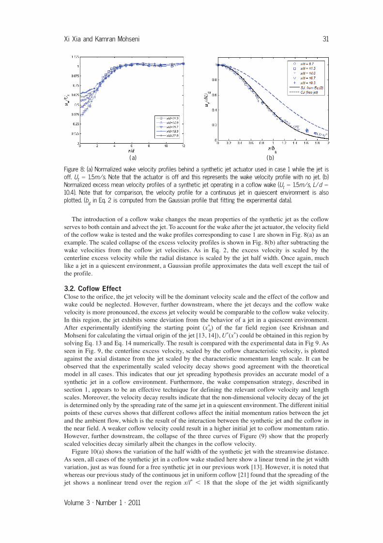
The introduction of a coflow wake changes the mean properties of the synthetic jet as the coflowserves to both contain and advect the jet. To account for the wake after the jet actuator, the velocity fieldof the coflow wake is tested and the wake profiles corresponding to case 1 are shown in Fig. 8(a) as anexample. The scaled collapse of the excess velocity profiles is shown in Fig. 8(b) after subtracting thewake velocities from the coflow jet velocities. As in Eq. 2, the excess velocity is scaled by thecenterline excess velocity while the radial distance is scaled by the jet half width. Once again, muchlike a jet in a quiescent environment, a Gaussian profile approximates the data well except the tail ofthe profile.

3.2. Coflow Effect

Close to the orifice, the jet velocity will be the dominant velocity scale and the effect of the coflow andwake could be neglected. However, further downstream, where the jet decays and the coflow wakevelocity is more pronounced, the excess jet velocity would be comparable to the coflow wake velocity.In this region, the jet exhibits some deviation from the behavior of a jet in a quiescent environment.After experimentally identifying the starting point (x*

0) of the far field region (see Krishnan andMohseni for calculating the virtual origin of the jet [13, 14]), U*(x*) could be obtained in this region bysolving Eq. 13 and Eq. 14 numerically. The result is compared with the experimental data in Fig 9. Asseen in Fig. 9, the centerline excess velocity, scaled by the coflow characteristic velocity, is plottedagainst the axial distance from the jet scaled by the characteristic momentum length scale. It can beobserved that the experimentally scaled velocity decay shows good agreement with the theoreticalmodel in all cases. This indicates that our jet spreading hypothesis provides an accurate model of asynthetic jet in a coflow environment. Furthermore, the wake compensation strategy, described insection 1, appears to be an effective technique for defining the relevant coflow velocity and lengthscales. Moreover, the velocity decay results indicate that the non-dimensional velocity decay of the jetis determined only by the spreading rate of the same jet in a quiescent environment. The different initialpoints of these curves shows that different coflows affect the initial momentum ratios between the jetand the ambient flow, which is the result of the interaction between the synthetic jet and the coflow inthe near field. A weaker coflow velocity could result in a higher initial jet to coflow momentum ratio.However, further downstream, the collapse of the three curves of Figure (9) show that the properlyscaled velocities decay similarly albeit the changes in the coflow velocity.

Figure 10(a) shows the variation of the half width of the synthetic jet with the streamwise distance.As seen, all cases of the synthetic jet in a coflow wake studied here show a linear trend in the jet widthvariation, just as was found for a free synthetic jet in our previous work [13]. However, it is noted thatwhereas our previous study of the continuous jet in uniform coflow [21] found that the spreading of thejet shows a nonlinear trend over the region x/l* � 18 that the slope of the jet width significantly



)b()a(

Figure 8: (a) Normalized wake velocity profiles behind a synthetic jet actuator used in case 1 while the jet isoff. Ut � 1.5m/s. Note that the actuator is off and this represents the wake velocity profile with no jet. (b)Normalized excess mean velocity profiles of a synthetic jet operating in a coflow wake (Ut � 1.5m/s, L/d �

10.4). Note that for comparison, the velocity profile for a continuous jet in quiescent environment is alsoplotted. (bg in Eq. 2 is computed from the Gaussian profile that fitting the experimental data).

deflected at the region x/l* 10; in this investigation, the flow field is measured over a regioncorresponding to x/l* � 8, and so the spreading of the synthetic jet may still be treated as linear. Thisindicates that the spreading of a synthetic jet in a coflow wake may be characterized by a singleconstant coefficient, namely the spreading rate (βg). Figure 10(b) shows the corresponding spreadingrates for the three cases considered. Here, the coflow variation is accounted for by a momentum fluxratio (Uj

2/Ut2), which is the ratio of the synthetic jet exit average momentum flux to the average coflow

momentum flux. In these three cases, Ut is varied while Uj remains constant. From observation, it isclear that the spreading rates of synthetic in coflow are smaller than that of a same synthetic in



Figure 9: Normalized centerline velocity decay (∆Ug/Ua) as a function of the scaled streamwise distance(x/l*) for cases 1, 2 and 3. Analytical solution for synthetic jets (SJ) solved from our model in equations13 and 14 is also plotted for comparison.

Figure 10: (a) Jet half width, bg, as a function of the non-dimensional streamwise distance x for cases 1, 2,3 and free synthetic jet; (b) Spreading rate change with coflow wake. The coflow velocity is converted tomomentum flux ratio and expressed as (Uj /Ut) . Note that βg for synthetic jets with Ut � 0 (quiescentenvironment, corresponding to infinity in this diagram), is 0.167.

quiescent flow. Further observation indicates that the presence of the coflow decreases the spreading ofthe synthetic jet to values that are even smaller than that of the spreading rate for a free continuous jet.Another point to note is that the spreading rate decreases as the coflow velocity increases. A possibleexplanation for this is that the existence of the coflow reduces the relative velocity jump across theshear layer of the jet and results in less shear layer energetics and less entrainment of the ambient flowby the jet; therefore, causing a weaker spreading of the jet.

3.3. Effect of Jet Strength

Besides the magnitude of the coflow wake velocity, the strength of the synthetic jet itself also plays arole in characterizing the flow. Here, the synthetic jet strength is changed by adjusting the input voltage,and the resultant strength may be characterized either using the value of L/d or the momentum flux ratio(Uj

2/Ut2). The larger the momentum flux ratio the higher the jet strength. Figure 11(a) shows the

centerline excess velocity decay with streamwise distance for different strengths of the synthetic jet inthe same coflow wake. Again, the experimental data shows good agreement with the theoretical model.This verifies the validity of our previous hypothesis and assumptions made to extend the continuous jetmodel to synthetic jets in coflow wake. A comparison of the velocity decay plots for several cases showsthat a stronger jet decays faster than a weaker one in the same coflow. Furthermore, stronger jets havelarger initial momentum ratios with respect to the coflow. This faster decay rate of stronger synthetic jetscan be attributed to a larger velocity difference between the jet and the ambient coflow, which causes thejet to entrain more fluid. The spreading rates for synthetic jets with and without a coflow are shown inFigure 11(b). These results confirms our previous observation that the coflow would decrease thespreading rate of a synthetic jet. Like the trend of synthetic jets in quiescent flow, a stronger jet increasesthe spreading rate of the synthetic jet. As stated previously, this is caused by the enhanced massentrainment from the ambient. It should be noted that, although adjusting the jet strength or the coflowvelocity would both change the initial momentum ratio and affect the jet spreading and decay, it isactually the jet strength that determines the spreading and decay rate while the coflow affects only theinitial condition and the velocity and length scales.

4. CONCLUSIONS

The flow field of a synthetic jet in a background flow is investigated using hot wire anemometry. Anintegral model similar to that employed in modeling continuous jets in a coflow is shown to be applicableto synthetic jets with some adjustments for the enhanced spreading rate of a synthetic jet and a wakecompensation for the flow actuator. The excess velocity profile of a synthetic jet in a coflow demonstratesself-similar behavior when scaled with the characteristic velocity and length scales obtained from acalculated top hat velocity profile. The model for the streamwise velocity decay shows good agreementwith experimental data for different coflow velocities and jet strengths. This model indicates that, in the



)b()a(

Figure 11: (a) Normalized centerline velocity decay as a function of the scaled streamwise distance forcases 1, 4 and 5; (b) Spreading rate change with the jet strength for synthetic jet in coflow wake. Thespreading rates of the synthetic jets with the same jet strengths with no coflow are also shown forcomparison. The jet strength is converted to momentum flux ratio, which is expressed as (Uj /Ut)

2.

far field, the non-dimensional velocity decay of a synthetic jet in a coflow is mostly determined by thespreading rate of that synthetic jet in quiescent environment. The effect of different coflow velocities onthis model is reflected by the different initial values of the non-dimensional velocities at the beginning ofthe far field. The observed decrease in the spreading rate of the jet indicates that the existence of thecoflow decreases the spreading of the synthetic jet. Furthermore, increasing the jet strength, parametrizedby increasing L/d in this study, causes an enhancement in jet spreading. The model presented here can beused to model the mean characteristics of a synthetic jet issues into a coflow wake.

ACKNOWLEDGEMENTS

The authors would like to thank Gopi Krishnan for his contribution of establishing the previous theory.The authors would like to thank Matthew Shields and Jill Cooper for their help in post-editing. Theauthors would like to acknowledge partial support from the Air Force Office of Scientific Research.

REFERENCES

[1] Smith, B. and Glezer, A., 1998, “The formation and evolution of synthetic jets,” Phys. Fluids,10(9), pp. 2281–2297.

[2] Glezer, A. and Amitay, M., 2002, “Synthetic jets,” Ann. Rev. Fluid Mech., 34, pp. 503–529.

[3] Seifert, A., Eliahu, S., Greenblatt, D., and Wygnanski, I., 1998, “Use of piezoelectric actuators forairfoil separation control,” AIAA Journal, 36(8), pp. 1535–1537.

[4] Amitay, M., Smith, D. R., Kibens, V., Parekh, D., and Glezer, A., 2001, “Aerodynamic flow controlover an unconventional airfoil using synthetic jet actuators,” AIAA Journal, 39(3), pp. 361–370.

[5] Mohseni, K., 2006, “Pulsatile vortex generators for low-speed maneuvering of small underwatervehicles,” Ocean Engineerings, 33(16), pp. 2209–2223.

[6] Krieg, M. and Mohseni, K., 2008, “Thrust characterization of pulsatile vortex ring generators forlocomotion of underwater robots,” IEEE J. Oceanic Engineering, 33(2), pp. 123–132.

[7] Mohseni, K., 2001, “Guided capsule for wireless endoscopy, biopsy, and drug delivery,” Patent.

[8] Mohseni, K., 2007, “An steerable mechanism for wireless capsule endoscopy,” Proceedings ofthe 2nd Frontiers in Biomedical Devices Conference, ASME, Irvine, CA, pp. BioMed2007–38048.

[9] Honohan, A. M., Amitay, M., and Glezer, A., 2000, “Aerodynamic control using synthetic jets,”AIAA paper 2000–2401, Fluids 2000 Conference and Exhibit, Denver, CO.

[10] Mittal, R. and Rampunggoon, P., 2002, “On the virtual aeroshaping effect of synthetic jets,” Phys.Fluids, 14(4), pp. 1533–1536.

[11] Whitehead, J. and Gursul, I., 2006, “Interaction of synthetic jet propulsion with airfoilaerodynamics at low reynolds numbers,” AIAA J., 44(8), pp. 1753–1766.

[12] Rizetta, D. P., Visbal, M. R., and Stanek, M. J., 1998, “Numerical investigation of synthetic jetflow-fields,” AIAA Paper 98–2910.

[13] Krishnan, G. and Mohseni, K., 2009, “Axisymmetric synthetic jets: An experimental andtheoretical examination,” AIAA J., 47(10), pp. 2273–2283.

[14] Krishnan, G. and Mohseni, K., 2009, “An experimental and analytical investigation of rectangularsynthetic jets,” ASME J. Fluid Eng., 131(12).

[15] Ugrina, S., 2007, Experimental analysis and analytical modeling of synthetic jet cross flowinteraction, Ph.D. thesis, University of Maryland.

[16] Xia, X. and Mohseni, K., 2010, “Modeling and experimental investigation of synthetic jets incross-flow,” AIAA paper 2010-0106, 48th AIAA Aerospace Sciences Meeting Including the NewHorizons Forum and Aerospace Exposition, Orlando, FL.

[17] Krueger, P., Dabiri, J., and Gharib, M., 2006, “The formation number of vortex rings formed in auniform background co-flow,” Journal of Fluid Mechanics, 556(1), pp. 147–166.

[18] Mallinson, S., Hong, G., and Reizes, J., 1999, “Some characteristics of synthetic jets,” AIAApaper 1999–3651, Norfolk, VA, proceedings of the 30th AIAA Fluid Dynamics Conference.

[19] Antonia, R. and Bilger, R., 1973, “Experimental investigation of an axisymmetric jet in a co-flowing air stream,” J. Fluid Mech, 61, pp. 805–822.



[20] Nickels, T. and Perry, A., 1996, “An experimental and theoretical study of the turbulent coflowingjet,” J. Fluid Mech, 309, pp. 157–182.

[21] Chu, P., Lee, J., and Chu, V., 1999, “Spreading of turbulent round jet in coflow,” Journal ofHydraulic Engineerings, 125, pp. 193–204.

[22] Squire, H. and Trouncer, J., 1944, “Round jets in a general stream,” Tech. rep., Aero ResearchCouncil, London, UK.

[23] Hill, P., 1965, “Turbulent jets in ducted streams,” J. Fluid Mech, 22, pp. 161–186.

[24] Patel, R., 1971, “Turbulent jets and wall jets in uniform streaming flow,” Aeronautical Quarterly,22, pp. 311–326.

[25] Morton, B., 1962, “Coaxial turbulent jets,” Int. J. Heat Mass Transfer, 5, pp. 955–965.

[26] Maczynski, J., 1962, “A round jet in an ambient co-axial stream,” J. Fluid Mech, 13, pp. 597–608.

[27] Krishnan, G. and Mohseni, K., 2010, “An experimental study of a radial wall jet formed by thenormal impingement of a round synthetic jet,” European Journal of Mechanics B/Fluids, 29,pp. 269–277.

[28] Kotsovinos, N. and Angelidis, P., 1991, “The momentum flux in turbulent submerged jets,”J. Fluid Mech, 229, pp. 453–470.

[29] Schlichting, H., 1933, “Laminare strahlausbreitung,” J. Appl. Math. Mech. (ZAMM), 13,pp. 260–263.

[30] Schlichting, H., 1979, Boundary-Layer Theory, McGraw-Hill Book Company, New York.

[31] Fugal, S. R., Smith, B. L., and Spall, R. E., 2005, “Displacement amplitude scaling of a two-dimensional synthetic jet,” Physics of Fluids, 17(4), pp. 045103–1–10.

[32] Pope, S., 2000, Turbulent Flows, Cambridge University Press, New York.

[33] Smith, B. and Swift, G., 2001, “Synthetic jets at larger reynolds number and comparison tocontinuous jets,” AIAA paper AIAA 2001-3030, Anaheim, CA, 31st AIAA Fluid DynamicsConference and Exhibit.

[34] Shuster, J. and Smith, D., 2007, “Experimental study of the formation and scaling of a roundsynthetic jet,” Physics of Fluids, 19(4), pp. 45109–1–21.

[35] Johnstone, A., Uddin, M., and Pollard, A., 2005, “Calibration of hot-wire probes using non-uniform mean velocity profiles,” Experiments in Fluids, 39(3), pp. 525–532.



Documents

Reprinted from International Journal of Flow Control