Embed Size (px)
Citation preview
In QuantItatIve Methods In PaleobIology, PP. 19-54, PaleontologIcal socIety short course, october 30th, 2010. the PaleontologIcal socIety PaPers, voluMe 16, John alroy and gene hunt (eds.). coPyrIght © 2010 the PaleontologIcal socIety
resaMPlIng Methods In PaleontologyMICHAŁ KOWALEWSKI
Department of Geosciences, Virginia Tech, Blacksburg, VA 24061
and
PHIL NOVACK-GOTTSHALL
Department of Biology, Benedictine University, 5700 College Road, Lisle, IL 60532
ABSTRACT.—This chapter reviews major types of statistical resampling approaches used in paleontology. They are an increasingly popular alternative to the classic parametric approach because they can approximate behaviors of parameters that are not understood theoretically. The primary goal of most resampling methods is an empirical approximation of a sampling distribution of a statistic of interest, whether simple (mean or standard error) or more complicated (median, kurtosis, or eigenvalue). This chapter focuses on the conceptual and practical aspects of resampling methods that a user is likely to face when designing them, rather than the relevant math-ematical derivations and intricate details of the statistical theory. The chapter reviews the concept of sampling distributions, outlines a generalized methodology for designing resampling methods, summarizes major types of resampling strategies, highlights some commonly used resampling protocols, and addresses various practical decisions involved in designing algorithm details. A particular emphasis has been placed here on bootstrapping, a resampling strategy used extensively in quantitative paleontological analyses, but other resampling techniques are also reviewed in detail. In addition, ad hoc and literature-based case examples are provided to illustrate virtues, limitations, and potential pitfalls of resampling methods.
We can formulate bootstrap simulations for almost any conceivable problem. Once we program the computer to carry out the bootstrap replications, we let the com-puter do all the work. A danger of this approach is that a practitioner might bootstrap at will, without consulting a statistician (or considering statistical implications) and without giving careful thought to the problem.
—Michael R. Chernick (2007, p. 13)
IntroductIon
RESAMPLING METHODS represent a family of com-puter-based strategies that can be used to standardize samples, test statistical hypotheses, estimate standard errors and confidence limits, develop cross-validation assessments, compare likelihood models, and carry out other types of statistical evaluations of empirical data sets. These methods rely primarily on iterative manipu-lations of data that typically involve direct resampling of observations, or, less frequently, projections of ran-dom data sets onto preexisting sample structures. This chapter aims to provide a general introduction to these
methods from a practical, paleontological perspective.In largely inductive sciences, such as biology or
paleontology, statistical evaluation of empirical data, whether exploratory or confirmatory, forms the meth-odological core of research. It is thus not surprising that resampling methods have spread widely into biosci-ences, quickly becoming one of its important statistical tools. There are multiple reasons for this success. First, resampling methods can be used in lieu of virtually any traditional parametric statistical method when that classic method works. Second, and more important, the resampling approaches can be also used in cases when the classic methods do not work, such as cases when assumptions of parametric methods are violated. Finally, and perhaps most important, the resampling methods can be used to evaluate statistical questions for which neither statistical theory nor parametric tests are available. Thus, for example, resampling methods may allow us to estimate a standard error of the eigenvalue of the first principal component, which is something that classic statistical methods cannot address readily (see Diaconis and Efron, 1983). Of course, as highlighted
20 the PaleontologIcal socIety PaPers, vol.16
below, resampling methods are not without problems or assumptions. However, there are many situations in which they can aid statistical treatment of data.
We hope to provide here a general introduction for those interested in learning more about resampling methods and their paleontological applications. Obvi-ously, a comprehensive, exhaustive treatment of such a broad subject is impossible in a single chapter. Here we focus primarily on practical issues a paleontologist may face when designing resampling strategies. To this end, we have compiled a reasonably comprehensive list of practical questions one needs to answer when designing resampling methods or when evaluating paleontological papers that use such methods. We have not included detailed mathematical derivations or theoretical justifications for various approaches exemplified below. Instead, we direct those who intend to use resampling methods in their research to consult textbooks for a detailed, but accessible, treatment of the subject (e.g., Hjorth, 1994; Davison and Hinkley, 1997; Efron and Tibshirani, 1997; Manly, 2004; Chernick, 2007; Edgington and Onghena, 2007). In the hope of maximizing practical utility and transparency of the chapter, we use below simple examples, figures, and generalized algorithm recipes that can help beginners to enter the conceptual world of resampling methods. A glossary of terms is provided in Appendix 1 in order to facilitate understanding of terms that are used often in the literature, but not always consistently. In addi-tion, supplementary online materials can be accessed at http://paleosoc.org/shortcourse2010.html, including codes written in R (contact PN-G with questions) and SAS/IML (contact MK with questions) that readers are welcome to use when assembling their resampling tool kits (appendices also include additional codes and content not cited in the text).
saMPlIng dIstrIbutIons
To explain resampling methods, we first need to review the concept of sampling distributions, which form the core of the classic parametric statistical ap-proach. They are used primarily to test hypotheses by probabilistic assessment of the observed values of statistics (e.g., the arithmetic mean, the Pearson’s correlation coefficient, etc.) or to estimate confidence intervals and standard errors around such values. They are also the primary target of resampling methods.
Indeed, for the most part, resampling is nothing but an empirical way for deriving sampling distributions.
A sampling distribution is an expected frequency distribution of some statistic of interest sampled randomly at a given sample size, typically from a large, practically infinite population of observations. Sampling distributions are a key prerequisite for un-derstanding resampling methods, so let us explore this issue using a simple example.
Upon discovery of a 14th century burial site in Italy, with mummified remains of adult male monks, ten complete bodies were recovered and their heights were recorded as follows: 154, 157, 158, 161, 162, 162, 164, 171, 178, and 205 cm. Were 14th century Italian males shorter than their present-day descendents? According to Wikipedia the mean height of a modern Italian male is 176.0 cm. The mean height of these ten mummified monks is 167.2 cm. Can we demonstrate compellingly that those medieval males were shorter than their present-day counterparts?
Let us be generous and grant those researchers two statistical assumptions: (1) the monks are a random and representative sample of independent observations derived from the 14th century male population of Italy, and (2) the modern estimate of 176.0 cm is very ac-curate and precise, to the point that we can assume that 176.0 cm is the true population mean for contemporary Italians. Given those assumptions, the researchers still need to show that their data (i.e., ten long dead, perfectly mummified monks) could not have possibly come from a population of males that averaged 176.0 cm in height. Our null hypothesis therefore is that the true 14th C. population mean is 176.0 cm.
Statisticians using classical methods can esti-mate the probability of incorrectly rejecting that null hypothesis by computing the t-value (e.g., Sokal and Rohlf, 1995; Zar, 2009):
(1)
Here, µ is the mean postulated by the null hypoth-esis (176.0 cm), Y is the sample mean (167.2 cm), and SE is computed by dividing the standard deviation of the sample by the square root of the sample size. In our case, SE = 15.002/√10 = 4.744 cm. Once the t-value is computed (t = -1.85), the corresponding two-tailed p-value of incorrectly rejecting the true null hypothesis (p = 0.0966 in our case) for the appropriate number of
Eq. 1 t =Y - µSEEq. 1 t =
Y - µSE
KOWALEWSKI ANd NOVACK-GOTTSHALL—RESAMPLING METHOdS IN PALEONTOLOGy 21
degrees of freedom (df = n - 1 = 9) can be retrieved from appendices provided in introductory statistical text-books or built-in tables included in statistical software.
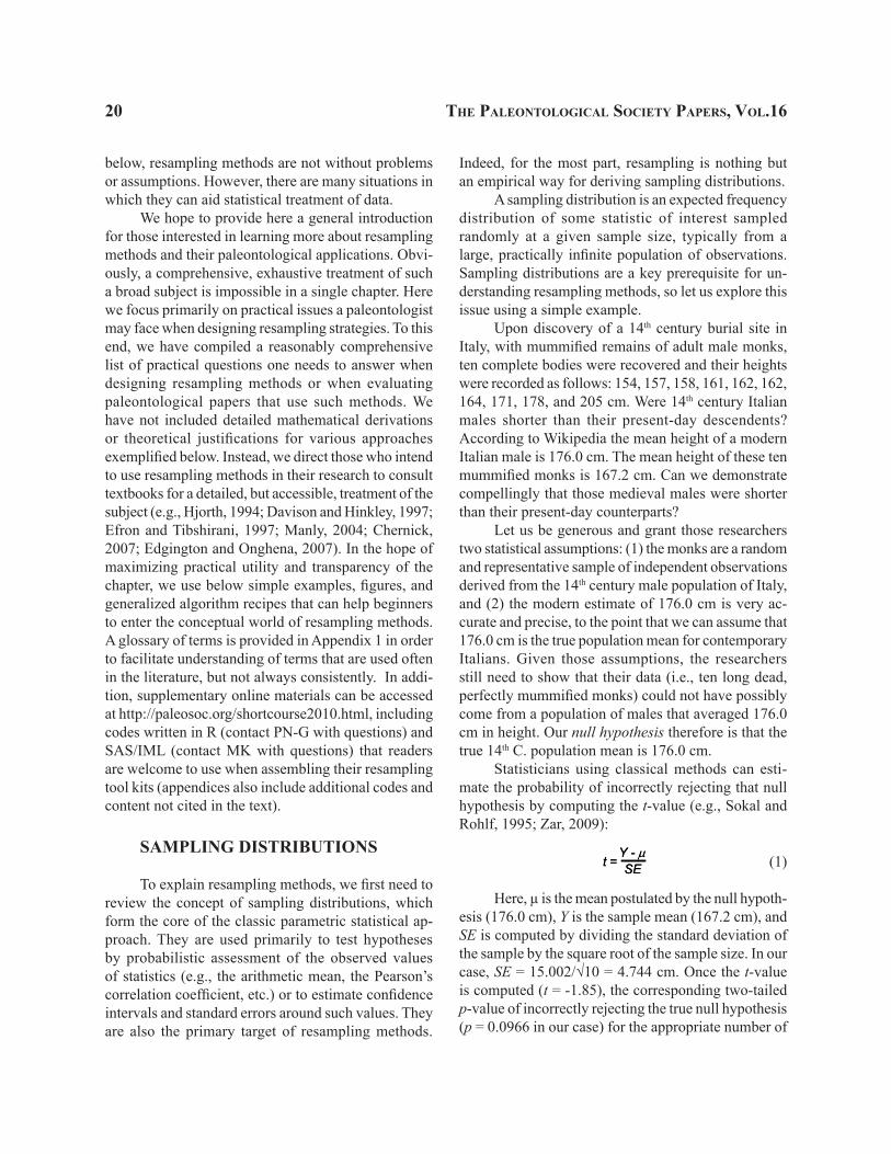
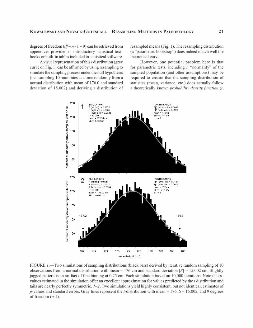
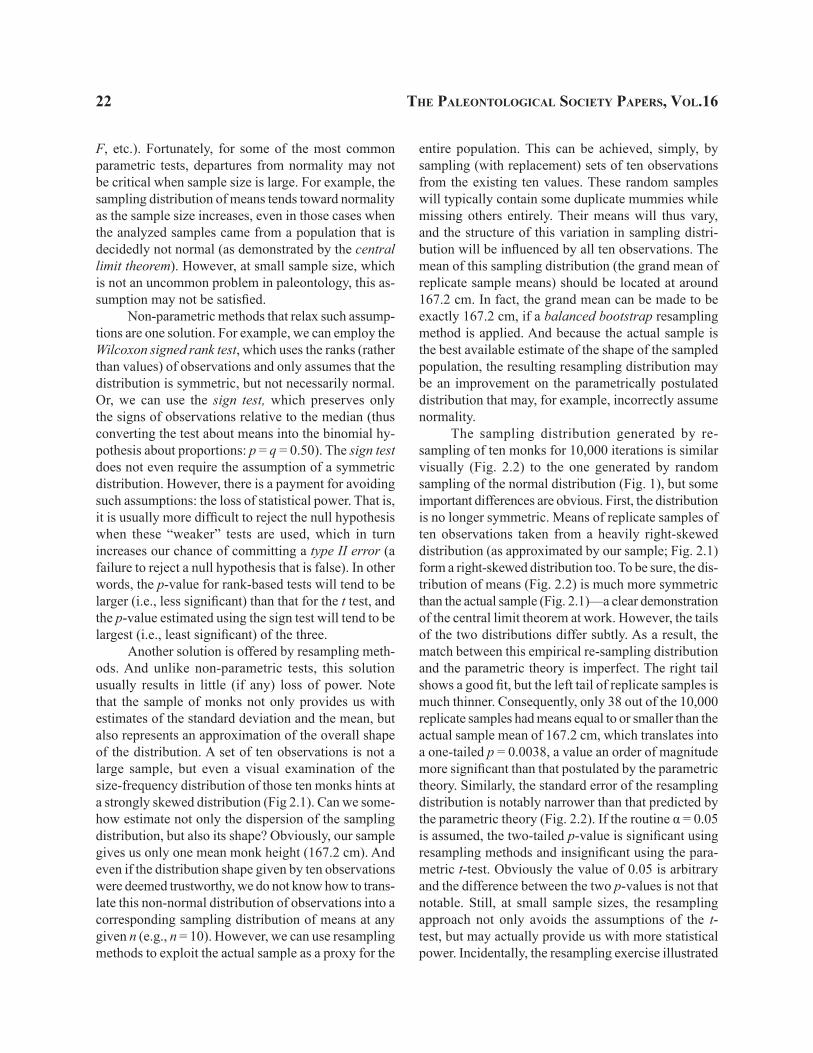
A visual representation of this t distribution (gray curve on Fig. 1) can be affirmed by using resampling to simulate the sampling process under the null hypothesis (i.e., sampling 10 mummies at a time randomly from a normal distribution with mean of 176.0 and standard deviation of 15.002) and deriving a distribution of
resampled means (Fig. 1). The resampling distribution (a “parametric bootstrap”) does indeed match well the theoretical curve.
However, one potential problem here is that for parametric tests, including t, “normality” of the sampled population (and other assumptions) may be required to ensure that the sampling distribution of statistics (mean, variance, etc.) does actually follow a theoretically known probability density function (t,
FIGURE 1.—Two simulations of sampling distributions (black bars) derived by iterative random sampling of 10 observations from a normal distribution with mean = 176 cm and standard deviation [S] = 15.002 cm. Slightly jagged pattern is an artifact of fine binning at 0.25 cm. Each simulation based on 10,000 iterations. Note that p-values estimated in the simulation offer an excellent approximation for values predicted by the t distribution and tails are nearly perfectly symmetric. 1–2, Two simulations yield highly consistent, but not identical, estimates of p-values and standard errors. Gray lines represent the t-distribution with mean = 176, S = 15.002, and 9 degrees of freedom (n-1).
22 the PaleontologIcal socIety PaPers, vol.16
F, etc.). Fortunately, for some of the most common parametric tests, departures from normality may not be critical when sample size is large. For example, the sampling distribution of means tends toward normality as the sample size increases, even in those cases when the analyzed samples came from a population that is decidedly not normal (as demonstrated by the central limit theorem). However, at small sample size, which is not an uncommon problem in paleontology, this as-sumption may not be satisfied.
Non-parametric methods that relax such assump-tions are one solution. For example, we can employ the Wilcoxon signed rank test, which uses the ranks (rather than values) of observations and only assumes that the distribution is symmetric, but not necessarily normal. Or, we can use the sign test, which preserves only the signs of observations relative to the median (thus converting the test about means into the binomial hy-pothesis about proportions: p = q = 0.50). The sign test does not even require the assumption of a symmetric distribution. However, there is a payment for avoiding such assumptions: the loss of statistical power. That is, it is usually more difficult to reject the null hypothesis when these “weaker” tests are used, which in turn increases our chance of committing a type II error (a failure to reject a null hypothesis that is false). In other words, the p-value for rank-based tests will tend to be larger (i.e., less significant) than that for the t test, and the p-value estimated using the sign test will tend to be largest (i.e., least significant) of the three.
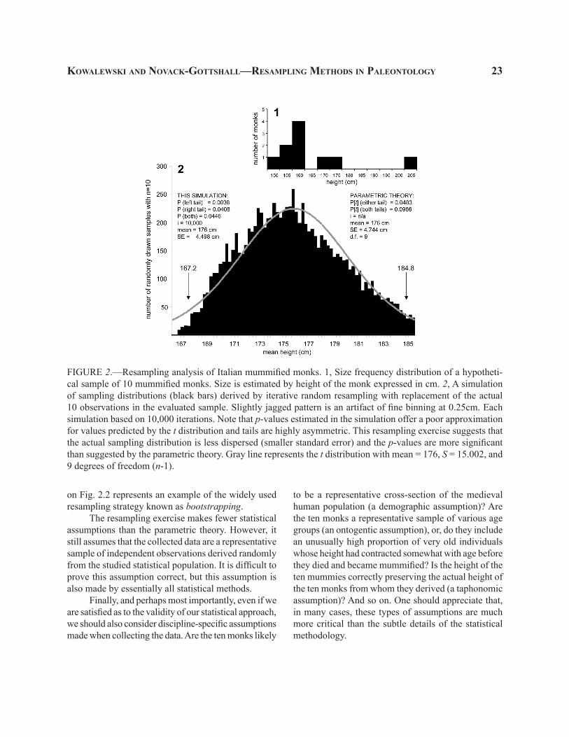
Another solution is offered by resampling meth-ods. And unlike non-parametric tests, this solution usually results in little (if any) loss of power. Note that the sample of monks not only provides us with estimates of the standard deviation and the mean, but also represents an approximation of the overall shape of the distribution. A set of ten observations is not a large sample, but even a visual examination of the size-frequency distribution of those ten monks hints at a strongly skewed distribution (Fig 2.1). Can we some-how estimate not only the dispersion of the sampling distribution, but also its shape? Obviously, our sample gives us only one mean monk height (167.2 cm). And even if the distribution shape given by ten observations were deemed trustworthy, we do not know how to trans-late this non-normal distribution of observations into a corresponding sampling distribution of means at any given n (e.g., n = 10). However, we can use resampling methods to exploit the actual sample as a proxy for the
entire population. This can be achieved, simply, by sampling (with replacement) sets of ten observations from the existing ten values. These random samples will typically contain some duplicate mummies while missing others entirely. Their means will thus vary, and the structure of this variation in sampling distri-bution will be influenced by all ten observations. The mean of this sampling distribution (the grand mean of replicate sample means) should be located at around 167.2 cm. In fact, the grand mean can be made to be exactly 167.2 cm, if a balanced bootstrap resampling method is applied. And because the actual sample is the best available estimate of the shape of the sampled population, the resulting resampling distribution may be an improvement on the parametrically postulated distribution that may, for example, incorrectly assume normality.
The sampling distribution generated by re-sampling of ten monks for 10,000 iterations is similar visually (Fig. 2.2) to the one generated by random sampling of the normal distribution (Fig. 1), but some important differences are obvious. First, the distribution is no longer symmetric. Means of replicate samples of ten observations taken from a heavily right-skewed distribution (as approximated by our sample; Fig. 2.1) form a right-skewed distribution too. To be sure, the dis-tribution of means (Fig. 2.2) is much more symmetric than the actual sample (Fig. 2.1)—a clear demonstration of the central limit theorem at work. However, the tails of the two distributions differ subtly. As a result, the match between this empirical re-sampling distribution and the parametric theory is imperfect. The right tail shows a good fit, but the left tail of replicate samples is much thinner. Consequently, only 38 out of the 10,000 replicate samples had means equal to or smaller than the actual sample mean of 167.2 cm, which translates into a one-tailed p = 0.0038, a value an order of magnitude more significant than that postulated by the parametric theory. Similarly, the standard error of the resampling distribution is notably narrower than that predicted by the parametric theory (Fig. 2.2). If the routine α = 0.05 is assumed, the two-tailed p-value is significant using resampling methods and insignificant using the para-metric t-test. Obviously the value of 0.05 is arbitrary and the difference between the two p-values is not that notable. Still, at small sample sizes, the resampling approach not only avoids the assumptions of the t-test, but may actually provide us with more statistical power. Incidentally, the resampling exercise illustrated
KOWALEWSKI ANd NOVACK-GOTTSHALL—RESAMPLING METHOdS IN PALEONTOLOGy 23
FIGURE 2.—Resampling analysis of Italian mummified monks. 1, Size frequency distribution of a hypotheti-cal sample of 10 mummified monks. Size is estimated by height of the monk expressed in cm. 2, A simulation of sampling distributions (black bars) derived by iterative random resampling with replacement of the actual 10 observations in the evaluated sample. Slightly jagged pattern is an artifact of fine binning at 0.25cm. Each simulation based on 10,000 iterations. Note that p-values estimated in the simulation offer a poor approximation for values predicted by the t distribution and tails are highly asymmetric. This resampling exercise suggests that the actual sampling distribution is less dispersed (smaller standard error) and the p-values are more significant than suggested by the parametric theory. Gray line represents the t distribution with mean = 176, S = 15.002, and 9 degrees of freedom (n-1).
on Fig. 2.2 represents an example of the widely used resampling strategy known as bootstrapping.
The resampling exercise makes fewer statistical assumptions than the parametric theory. However, it still assumes that the collected data are a representative sample of independent observations derived randomly from the studied statistical population. It is difficult to prove this assumption correct, but this assumption is also made by essentially all statistical methods.
Finally, and perhaps most importantly, even if we are satisfied as to the validity of our statistical approach, we should also consider discipline-specific assumptions made when collecting the data. Are the ten monks likely
to be a representative cross-section of the medieval human population (a demographic assumption)? Are the ten monks a representative sample of various age groups (an ontogentic assumption), or, do they include an unusually high proportion of very old individuals whose height had contracted somewhat with age before they died and became mummified? Is the height of the ten mummies correctly preserving the actual height of the ten monks from whom they derived (a taphonomic assumption)? And so on. One should appreciate that, in many cases, these types of assumptions are much more critical than the subtle details of the statistical methodology.
24 the PaleontologIcal socIety PaPers, vol.16
GENERAL FRAMEWORK FOR hyPothesIs testIng usIng
resaMPlIng Methods
While most standard statistical textbooks (e.g., Sokal and Rohlf, 1995; Zar, 2009) explain theoretical concepts and provide cookbook instruction for carrying out standard parametric and nonparametric analyses, this is not usually the case for resampling analyses. For such analyses, the burden is largely on users to combine their statistical knowledge and programming skills in order to develop an analytical solution catered to the analysis at hand. Fortunately, nearly all resampling (and standard statistical) analyses follow the same general pathway, which we present here and elaborate on during the rest of this chapter.
Identify the hypothesis.—It is critical to define, precisely, the hypothesis one wishes to evaluate. This can be in the form of a null hypothesis one attempts to falsify or a series of alternative hypotheses one seeks to compare. It is generally recommended at this stage to make additional decisions: Is a one- or two-tailed hypothesis warranted? What value of alpha (acceptable risk of committing type I error) is appropriate? Keep in mind though that the value of α (e.g., α = 0.05) is just a suggestion of how to make the decision and should not be followed religiously. The p-value is the actual measure of how strong your empirical evidence is against the null hypothesis. Arguably, p = 0.051 and p = 0.049 are telling us something very similar, and yet a dogmatic adherence to α = 0.05 would make them fundamentally different (see Siegfried, 2010 for a thoughtful and stimulating commentary).
Choose the appropriate statistical parameter for this hypothesis.—This can be a widely used statistical parameter, but any quantitative index may be sufficient (this flexibility is the key virtue of resampling meth-ods!). If testing whether two samples are different in terms of central tendency, the difference between means is adequate, just as it would be for a t-test. But, when evaluating more complex questions, one often needs to explore a variable of theoretically unknown statistical behavior, such as the maximum bin width in a histo-gram that turns a unimodal distribution into a bimodal distribution (see below) or the sample-standardized morphological disparity from a principal coordinates analysis.
Calculate the observed value of the sample statis-tic for your data.—The observed sample statistic will be later compared with the null resampling distribution (reference set) derived in your resampling protocol.
Produce a resampling distribution (reference set) by resampling your data.—Implement a data resam-pling method (or a theoretical randomization model in the case of some variants of Monte Carlo methods) appropriate to your hypothesis to rearrange, resample, model, or otherwise represent your data for many itera-tions (replications), determining the relevant value of the statistic at each iteration. Note that, in most cases, the sample size remains constant for each iteration (except when building rarefaction curves) and typi-cally matches the sample size of the actual data (except for jackknife, rarefaction, and sample-standardization methods). Thus, if resampling/modeling a sample of 24 observations, each resampled sample would ordinarily also have 24 observations. Step four is the only aspect of this framework that generally must be customized to your analyses, and many statistical programs offer standard functions. Finally, one needs to choose an ap-propriate number of iterations in the resampling routine that serves your required precision. The distribution of values of statistics derived in this step, referred to as the resampling distribution (or reference set), will form the basis for obtaining confidence intervals and p-values in step 5.
Calculate a p-value.—This is ordinarily done by comparing your observed sample statistic value computed in step 2 to the resulting resampling distri-bution of the resampled statistics derived in step 4, as you would do for any statistical hypothesis test. As noted below, it is often advisable to evaluate the power (sensitivity to type II error) of your analyses. Also, various corrections and adjustments may be necessary to minimize biases involved in estimating the p-value (some of those are itemized later in the text).
Wang (2003) offers an example of how to imple-ment this general framework. Wang was interested in whether there was continuity in extinction intensity between background and mass extinctions. He evalu-ated this question by examining the shape of the prob-ability density function (pdf, the continuous equivalent of a histogram) of Phanerozoic extinction intensities. If there was no discontinuity between extinction types
KOWALEWSKI ANd NOVACK-GOTTSHALL—RESAMPLING METHOdS IN PALEONTOLOGy 25
(his null hypothesis), the pdf would be unimodal. If a discontinuity existed (his alternative hypothesis), then the pdf would be bimodal or even multimodal. He recognized that the modality of an estimated pdf is sensitive to interval width (bandwidth): finer band-widths are likely to produce multiple modes. He thus chose as his test parameter the largest bandwidth that switches a unimodal distribution into a multimodal distribution. Because the sampling distribution of this critical bandwidth was unknown, Wang created a boot-strapped distribution (i.e., resampling distribution) of critical bandwidths to compare with his observed value, from which he calculated p-values to conclude that the distribution of Phanerozoic extinction intensities was unlikely to be discontinuous in terms of magnitude. Wang (2003) also conducted a test of the power of these analyses by manufacturing several extinction distributions that replicated the alternative hypothesis of bimodality between background and mass extinc-tions (each distribution varying in the magnitude of the discontinuity). He performed similar analyses as above, but as a measure of the test’s power, this time counted the number of times that the specified bimodal distribution was incorrectly demonstrated as unimodal.
tyPes oF resaMPlIng Methods
Terms denoting various types of resampling strategies (e.g., randomization, permutation test, bootstrapping, Monte Carlo) are used inconsistently in the literature. At the same time, the distinction be-tween seemingly different terms can be quite subtle (e.g., the distinction between permutation test and randomization test; see below), an issue amplified by sloppy nomenclatural adoptions by practitioners from other disciplines. Thus, in biology and paleontology, randomization is sometimes used as an umbrella term for any data-based resampling strategies and Monte Carlo is sometimes used to denote what others would consider a randomization or bootstrap test. To add to the confusion, the expression Monte Carlo approxima-tion is used to denote non-systematic (non-exhuastive) resampling that approximates complete enumeration estimates achievable by systematic (exhaustive) resa-mpling (the latter is possible when randomized data sets are very small).
Here we summarize the major types of resa-mpling methods. Our categorization partly follows
Manly’s (2004) comprehensive book on resampling methods written from a biological perspective (a glos-sary of the most important technical terms used here, noted in italics in the text, is provided in Appendix 1).
When broadly defined, resampling methods can be subdivided into several general categories. Except for one strategy (model-based, or implicit, Monte Carlo methods), the resampling strategies defined below rely primarily on drawing (whether by resampling, subsam-pling, or reshuffling) actual observations contained within empirical samples of interest. Six major fami-lies of resampling methods can be distinguished: (1) randomization, (2) bootstrapping, (3) jackknifing, (4) rarefaction and subsampling standardization, (5) data-based Monte Carlo, and (6) model-based Monte Carlo.
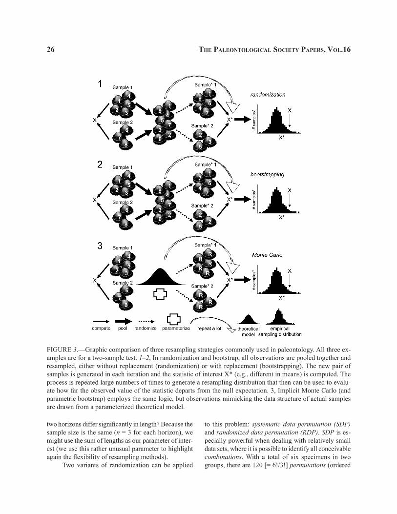
Randomization.—This term is used, typically, to denote resampling without replacement based on random re-assignment (re-ordering) of observations across groups, treatments, or samples (Fig. 3.1). Some authors use the term randomization interchangeably with the term permutation test; others view it as a subset of permutation methods, while some explicit recognize it as applicable primarily to experimental data (for more details see Efron and Tibshirani, 1997 and refer-ences therein; Manly, 2004; Good, 2006; Edgington and Onghena, 2007). These terminological nuances do not pertain so much to how one resamples data, but, rather, what type of data are being resampled and how the resampling results are being interpreted. Above all, one should keep in mind that randomization is a strategy designed primarily to deal with experimental data, such that statistical inference pertains only to the specific observations collected from experiments. Thus, randomization does not readily extrapolate results to the statistical populations from which those observations were acquired (see also Edgington and Onghena, 2007)
While particularly useful for experimental data, randomization is often applied to non-experimental data, even though statistical inference may be hampered in such cases. This is relevant for paleontology, where non-experimental data dominate and true randomness of samples is unlikely and difficult to demonstrate. Consider, for example, the case where a paleontologist collected six specimens of the trilobite Isotelus from two Late Ordovician horizons: 169, 173, and 178 mm long specimens in a lower horizon and 190, 193, and 209 mm in an upper one. Do the trilobites from these
26 the PaleontologIcal socIety PaPers, vol.16
two horizons differ significantly in length? Because the sample size is the same (n = 3 for each horizon), we might use the sum of lengths as our parameter of inter-est (we use this rather unusual parameter to highlight again the flexibility of resampling methods).
Two variants of randomization can be applied
FIGURE 3.—Graphic comparison of three resampling strategies commonly used in paleontology. All three ex-amples are for a two-sample test. 1–2, In randomization and bootstrap, all observations are pooled together and resampled, either without replacement (randomization) or with replacement (bootstrapping). The new pair of samples is generated in each iteration and the statistic of interest X* (e.g., different in means) is computed. The process is repeated large numbers of times to generate a resampling distribution that then can be used to evalu-ate how far the observed value of the statistic departs from the null expectation. 3, Implicit Monte Carlo (and parametric bootstrap) employs the same logic, but observations mimicking the data structure of actual samples are drawn from a parameterized theoretical model.
to this problem: systematic data permutation (SDP) and randomized data permutation (RDP). SDP is es-pecially powerful when dealing with relatively small data sets, where it is possible to identify all conceivable combinations. With a total of six specimens in two groups, there are 120 [= 6!/3!] permutations (ordered
KOWALEWSKI ANd NOVACK-GOTTSHALL—RESAMPLING METHOdS IN PALEONTOLOGy 27
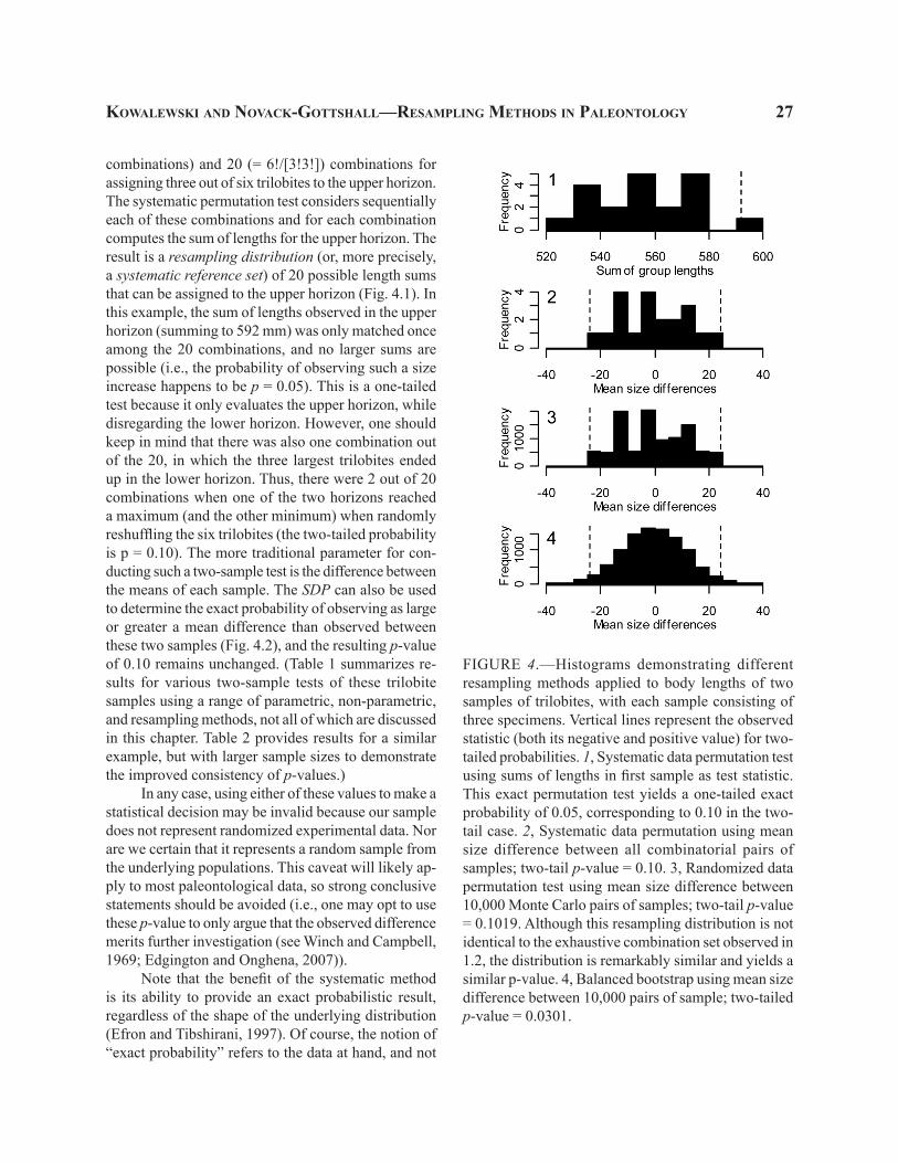
combinations) and 20 (= 6!/[3!3!]) combinations for assigning three out of six trilobites to the upper horizon. The systematic permutation test considers sequentially each of these combinations and for each combination computes the sum of lengths for the upper horizon. The result is a resampling distribution (or, more precisely, a systematic reference set) of 20 possible length sums that can be assigned to the upper horizon (Fig. 4.1). In this example, the sum of lengths observed in the upper horizon (summing to 592 mm) was only matched once among the 20 combinations, and no larger sums are possible (i.e., the probability of observing such a size increase happens to be p = 0.05). This is a one-tailed test because it only evaluates the upper horizon, while disregarding the lower horizon. However, one should keep in mind that there was also one combination out of the 20, in which the three largest trilobites ended up in the lower horizon. Thus, there were 2 out of 20 combinations when one of the two horizons reached a maximum (and the other minimum) when randomly reshuffling the six trilobites (the two-tailed probability is p = 0.10). The more traditional parameter for con-ducting such a two-sample test is the difference between the means of each sample. The SDP can also be used to determine the exact probability of observing as large or greater a mean difference than observed between these two samples (Fig. 4.2), and the resulting p-value of 0.10 remains unchanged. (Table 1 summarizes re-sults for various two-sample tests of these trilobite samples using a range of parametric, non-parametric, and resampling methods, not all of which are discussed in this chapter. Table 2 provides results for a similar example, but with larger sample sizes to demonstrate the improved consistency of p-values.)
In any case, using either of these values to make a statistical decision may be invalid because our sample does not represent randomized experimental data. Nor are we certain that it represents a random sample from the underlying populations. This caveat will likely ap-ply to most paleontological data, so strong conclusive statements should be avoided (i.e., one may opt to use these p-value to only argue that the observed difference merits further investigation (see Winch and Campbell, 1969; Edgington and Onghena, 2007)).
Note that the benefit of the systematic method is its ability to provide an exact probabilistic result, regardless of the shape of the underlying distribution (Efron and Tibshirani, 1997). Of course, the notion of “exact probability” refers to the data at hand, and not
FIGURE 4.—Histograms demonstrating different resampling methods applied to body lengths of two samples of trilobites, with each sample consisting of three specimens. Vertical lines represent the observed statistic (both its negative and positive value) for two-tailed probabilities. 1, Systematic data permutation test using sums of lengths in first sample as test statistic. This exact permutation test yields a one-tailed exact probability of 0.05, corresponding to 0.10 in the two-tail case. 2, Systematic data permutation using mean size difference between all combinatorial pairs of samples; two-tail p-value = 0.10. 3, Randomized data permutation test using mean size difference between 10,000 Monte Carlo pairs of samples; two-tail p-value = 0.1019. Although this resampling distribution is not identical to the exhaustive combination set observed in 1.2, the distribution is remarkably similar and yields a similar p-value. 4, Balanced bootstrap using mean size difference between 10,000 pairs of sample; two-tailed p-value = 0.0301.
28 the PaleontologIcal socIety PaPers, vol.16
the sampled population. Thus, it applies primarily to experimental data, where experimental observations and not underlying populations are being evaluated.
Randomized data permutation (RDP, called “sampled randomization” by Sokal and Rohlf, 1995) is a practical solution when data are too large for sys-tematic permutation. Although computers can often handle immense numbers of iterations, the number of permutations increases dramatically with sample size (see also Fig. 7). For example, systematic data permutation would require 20 [= 6!/3!3!] combinations in a case involving two samples with three trilobites in each, but 184,756 [= 20!/(10!10!)] combinations if each sample had ten trilobites. Fortunately, randomized data permutation can make the randomization process manageable by random resampling of a subset of all
possible permutations (note that RDP is a Monte Carlo approximation of SDP).
Although the SDP test is practical for this small case example, it is worth examining the randomized data permutation here to demonstrate that it provides a reasonable alternative. To perform RDP, we can ran-domly reassign trilobites to two horizons and repeat this process, say, 10,000 times to create 10,000 sets of six randomly permuted trilobites. The resulting resampling distribution (Fig. 4.3) represents a Monte Carlo approximation of the systematic reference set (Fig. 4.2) computed using SDP described above. The p-value can then be derived by evaluating how many randomly permutated samples yielded a mean size dif-ference that equals or exceeds the sample statistic. In the example shown here (Fig. 4.3), 1,019 out of 10,000
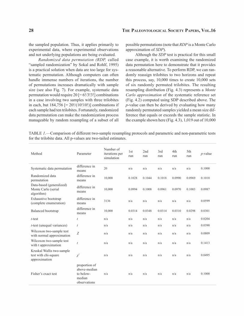
TABLE 1.—Comparison of different two-sample resampling protocols and parametric and non-parametric tests for the trilobite data. All p-values are two-tailed estimates.
Method ParameterNumber of iterations per simulation
1st run
2nd run
3rd run
4th run
5th run p-value
Systematic data permutation difference in means 20 n/a n/a n/a n/a n/a 0.1000
Randomized data permutation
difference in means 10,000 0.1028 0.1044 0.1018 0.0990 0.0969 0.1010
Data-based (generalized) Monte Carlo (serial algorithm)
difference in means 10,000 0.0994 0.1008 0.0961 0.0970 0.1003 0.0987
Exhaustive bootstrap (complete enumeration)
difference in means 3136 n/a n/a n/a n/a n/a 0.0599
Balanced bootstrap difference in means 10,000 0.0314 0.0348 0.0314 0.0310 0.0298 0.0301
t-test t n/a n/a n/a n/a n/a n/a 0.0204
t-test (unequal variances) t n/a n/a n/a n/a n/a n/a 0.0390
Wilcoxon two-sample test with normal approximation Z n/a n/a n/a n/a n/a n/a 0.0809
Wilcoxon two-sample test with t approximation t n/a n/a n/a n/a n/a n/a 0.1413
Kruskal Wallis two-sample test with chi-square approximation
χ2 n/a n/a n/a n/a n/a n/a 0.0495
Fisher’s exact test
proportion of above-median to below- median observations
n/a n/a n/a n/a n/a n/a 0.1000
KOWALEWSKI ANd NOVACK-GOTTSHALL—RESAMPLING METHOdS IN PALEONTOLOGy 29
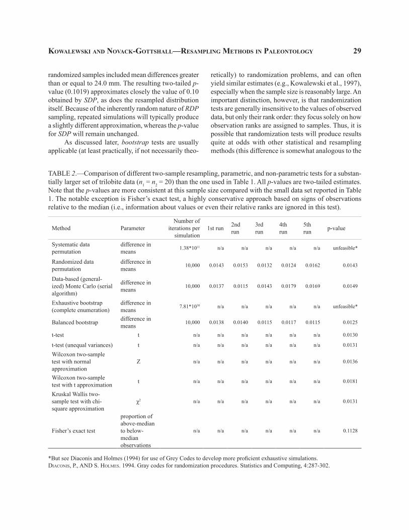
TABLE 2.—Comparison of different two-sample resampling, parametric, and non-parametric tests for a substan-tially larger set of trilobite data (n1 = n2 = 20) than the one used in Table 1. All p-values are two-tailed estimates. Note that the p-values are more consistent at this sample size compared with the small data set reported in Table 1. The notable exception is Fisher’s exact test, a highly conservative approach based on signs of observations relative to the median (i.e., information about values or even their relative ranks are ignored in this test).
Method ParameterNumber of
iterations per simulation
1st run 2nd run
3rd run
4th run
5th run p-value
Systematic data permutation
difference in means 1.38*1011 n/a n/a n/a n/a n/a unfeasible*
Randomized data permutation
difference in means 10,000 0.0143 0.0153 0.0132 0.0124 0.0162 0.0143
Data-based (general-ized) Monte Carlo (serial algorithm)
difference in means 10,000 0.0137 0.0115 0.0143 0.0179 0.0169 0.0149
Exhaustive bootstrap (complete enumeration)
difference in means 7.81*1030 n/a n/a n/a n/a n/a unfeasible*
Balanced bootstrap difference in means 10,000 0.0138 0.0140 0.0115 0.0117 0.0115 0.0125
t-test t n/a n/a n/a n/a n/a n/a 0.0130
t-test (unequal variances) t n/a n/a n/a n/a n/a n/a 0.0131
Wilcoxon two-sample test with normal approximation
Z n/a n/a n/a n/a n/a n/a 0.0136
Wilcoxon two-sample test with t approximation t n/a n/a n/a n/a n/a n/a 0.0181
Kruskal Wallis two- sample test with chi-square approximation
χ2 n/a n/a n/a n/a n/a n/a 0.0131
Fisher’s exact test
proportion of above-median to below- median observations
n/a n/a n/a n/a n/a n/a 0.1128
*But see Diaconis and Holmes (1994) for use of Grey Codes to develop more proficient exhaustive simulations.DIACONIS, P., AND S. HOLMES. 1994. Gray codes for randomization procedures. Statistics and Computing, 4:287-302.
randomized samples included mean differences greater than or equal to 24.0 mm. The resulting two-tailed p-value (0.1019) approximates closely the value of 0.10 obtained by SDP, as does the resampled distribution itself. Because of the inherently random nature of RDP sampling, repeated simulations will typically produce a slightly different approximation, whereas the p-value for SDP will remain unchanged.
As discussed later, bootstrap tests are usually applicable (at least practically, if not necessarily theo-
retically) to randomization problems, and can often yield similar estimates (e.g., Kowalewski et al., 1997), especially when the sample size is reasonably large. An important distinction, however, is that randomization tests are generally insensitive to the values of observed data, but only their rank order: they focus solely on how observation ranks are assigned to samples. Thus, it is possible that randomization tests will produce results quite at odds with other statistical and resampling methods (this difference is somewhat analogous to the
30 the PaleontologIcal socIety PaPers, vol.16
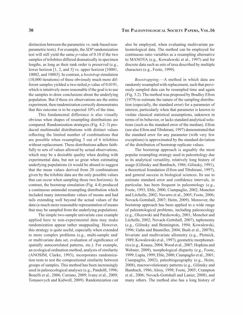
distinction between the parametric vs. rank-based non-parametric tests). For example, the SDP randomization test will still yield the same p-value of 0.10 if the two samples of trilobites differed dramatically in specimen lengths, as long as their rank order is preserved (e.g., lower horizon [1, 2, and 3] vs. upper horizon [10001, 10002, and 10003]. In contrast, a bootstrap simulation (10,000 iterations) of these obviously much more dif-ferent samples yielded a two-tailed p-value of 0.0191, which is intuitively more reasonable if the goal is to use the samples to draw conclusions about the underlying population. But if these six observations are the entire experiment, then randomization correctly demonstrates that this outcome is to be expected 10% of the time.
This fundamental difference is also visually obvious when shapes of resampling distributions are compared. Randomization strategies (Fig. 4.2–3) pro-duced multimodal distributions with distinct values reflecting the limited number of combinations that are possible when resampling 3 out of 6 trilobites without replacement. These distributions adhere faith-fully to sets of values allowed by actual observations, which may be a desirable quality when dealing with experimental data, but not so great when estimating underlying populations (it would be absurd to suggest that the mean values derived from 20 combinations given by the trilobite data are the only possible values that can occur when sampling those two horizons). In contrast, the bootstrap simulation (Fig. 4.4) produced a continuous unimodal resampling distribution which included many intermediate values of means and had tails extending well beyond the actual values of the data (a much more reasonable representation of means that may be sampled from the underlying population).
The simple two-sample univariate case example applied here to non-experimental data may make randomization appear rather unappealing. However, this strategy is quite useful, especially when extended to more complex problems (e.g., multi-sample and/or multivariate data set, evaluation of significance of spatially autocorrelated patterns, etc.). For example, an ecological ordination method, analysis of similarity (ANOSIM, Clarke, 1993), incorporates randomiza-tion tests to test the compositional similarity between groups of samples. This method has been increasingly used in paleoecological analyses (e.g., Pandolfi, 1996; Bonelli et al., 2006; Currano, 2009; Ivany et al., 2009; Tomasovych and Kidwell, 2009). Randomization can
also be employed, when evaluating multivariate pa-leontological data. The method can be employed for continuous ratio variables as a resampling alternative to MANOVA (e.g., Kowalewski et al., 1997) and for discrete data such as sets of taxa described by multiple characters (e.g., Foote, 1999).
Boostrapping.—A method in which data are randomly resampled with replacement, such that previ-ously sampled data can be resampled time and again (Fig. 3.2). The method was proposed by Bradley Efron (1979) to estimate the nature of the sampling distribu-tion (especially, the standard error) for a parameter of interest, particularly when that parameter is known to violate classical statistical assumptions, unknown in terms of its behavior, or lacks standard analytical solu-tions (such as the standard error of the median). Efron (see also Efron and Tibshirani, 1997) demonstrated that the standard error for any parameter (with very few exceptions) is approximated by the standard deviation of the distribution of bootstrap replicate values.
The bootstrap approach is arguably the most popular resampling strategy used in paleontology due to its analytical versatility, relatively long history of usage (Gilinsky and Bambach, 1986; Gilinsky, 1991), a theoretical foundation (Efron and Tibshirani, 1997), and general success in biological sciences. Its use to estimate standard error and confidence intervals, in particular, has been frequent in paleontology (e.g., Foote, 1993; Eble, 2000; Ciampaglio, 2002; Monchot and Léchelle, 2002; Navarro et al., 2005; Foote, 2006; Novack-Gottshall, 2007; Heim, 2009). Moreover, the bootstrap approach has been applied to a wide range of paleontological problems, including paleoecology (e.g., Olszewski and Patzkowsky, 2001; Monchot and Léchelle, 2002; Novack-Gottshall, 2007), taphonomy (e.g., Gilinsky and Bennington, 1994; Kowalewski, 1996; Gahn and Baumiller, 2004; Bush et al., 2007b), bivariate and multivariate allometry (e.g., Plotnick, 1989; Kowalewski et al., 1997), geometric morphomet-rics (e.g., Krause, 2004; Wood et al., 2007; Hopkins and Webster, 2009), morphological disparity (e.g., Foote, 1999; Lupia, 1999; Eble, 2000; Ciampaglio et al., 2001; Ciampaglio, 2002), paleobiogeography (e.g., Heim, 2008), macroevolutionary patterns (e.g., Gilinsky and Bambach, 1986; Alroy, 1998; Foote, 2005; Crampton et al., 2006; Novack-Gottshall and Lanier, 2008), and many others. The method also has a long history of
KOWALEWSKI ANd NOVACK-GOTTSHALL—RESAMPLING METHOdS IN PALEONTOLOGy 31
usage in phylogenetic analyses, primarily to evaluate the support for hypotheses of monophyly.
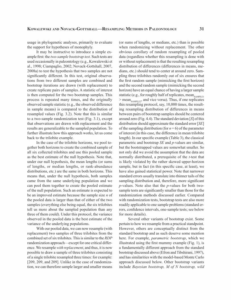
It may be instructive to introduce a simple ex-ample first: the two-sample bootstrap test. Such tests are used occasionally in paleontology (e.g., Kowalewski et al., 1998; Ciampaglio, 2002; Novack-Gottshall, 2007, 2008a) to test the hypothesis that two samples are not significantly different. In this test, original observa-tions from two different samples are combined and bootstrap iterations are drawn (with replacement) to create replicate pairs of samples. A statistic of interest is then computed for the two bootstrap samples. This process is repeated many times, and the originally observed sample statistic (e.g., the observed difference in sample means) is compared to the distribution of resampled values (Fig. 3.2). Note that this is similar to a two-sample randomization test (Fig. 3.1), except that observations are drawn with replacement and the results are generalizable to the sampled population. To further illustrate how this approach works, let us come back to the trilobite example.
In the case of the trilobite horizons, we pool to-gether both horizons to create the combined sample of all six collected trilobites and use this pooled sample as the best estimate of the null hypothesis. Note that, under our null hypothesis, the mean lengths (or sums of lengths, or median lengths, or rank-abundance distributions, etc.) are the same in both horizons. This means that, under the null hypothesis, both samples came from the same underlying population and we can pool them together to create the pooled estimate of the null population. Such an estimate is expected to be an improved estimate because the sample size n of the pooled data is larger than that of either of the two samples (everything else being equal, the six trilobites tell us more about the sampled population than any three of them could). Under this protocol, the variance observed in the pooled data is the best estimate of the variance of the underlying populations.
With our pooled data, we can now resample (with replacement) two samples of three trilobites from the combined set of six trilobites. This is similar to the RDP randomization approach—except for one critical differ-ence. We resample with replacement, and thus, it is now possible to draw a sample of three trilobites consisting of a single trilobite resampled three times: for example: [209, 209, and 209]. Unlike in the case of randomiza-tion, we can therefore sample larger and smaller means
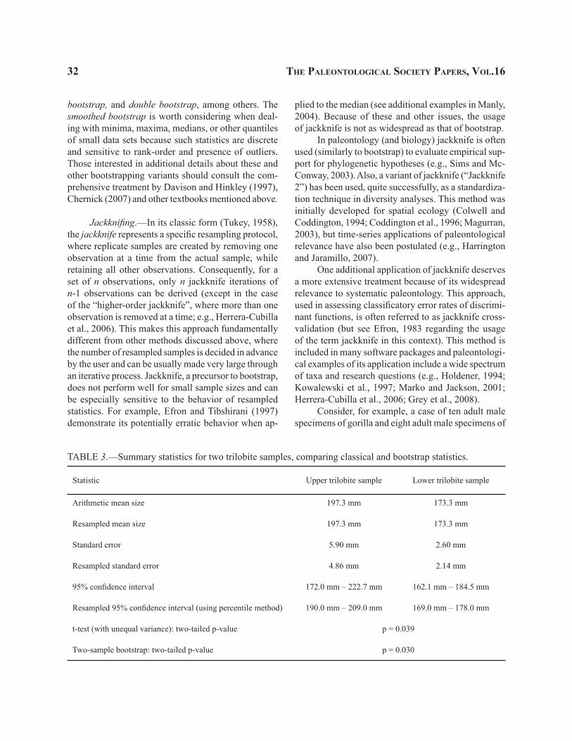
(or sums of lengths, or medians, etc.) than is possible when randomizing without replacement. The other obvious corollary of random resampling of pooled data (regardless whether this resampling is done with or without replacement) is that the resulting resampling distribution of differences (differences in means, me-dians, etc.) should tend to center at around zero. Sam-pling three trilobites randomly out of six ensures that the first random sample (mimicking the first horizon) and the second random sample (mimicking the second horizon) have an equal chance of having a larger sample statistic (e.g., for roughly half of replicates, meanSAMPLE1 > meanSAMPLE2, and vice versa). Thus, if one replicates this resampling protocol, say, 10,000 times, the result-ing resampling distribution of differences in means between pairs of bootstrap samples should be centered around zero (Fig. 4.4). The standard deviation [S] of this distribution should approximate the standard error [SE] of the sampling distribution (for n = 6) of the parameter of interest (in this case, the difference in mean trilobite length). In our specific example (Table 3), the classical parametric and bootstrap SE and p-values are similar, but the bootstrapped values are somewhat smaller. So not only did we avoid the assumption that the data are normally distributed, a prerequisite of the t-test that is likely violated by the rather skewed upper-horizon sample, but in fact (in this specific case, at least), we have also gained statistical power. Note that narrower standard errors usually translate into thinner tails of the sampling distribution and, therefore, more significant p-values. Note also that the p-values for both two-sample tests are significantly smaller than those for the randomization methods discussed earlier. Compared with randomization tests, bootstrap tests are also more readily applicable to one sample problems (standard er-rors, confidence intervals, one-sample tests; see below for more details).
Several other variants of bootstrap exist. Some pertain to how we resample from a practical standpoint. However, others are conceptually distinct from the standard bootstrap and as such deserve some mention here. For example, parametric bootstrap, which we illustrated using the first mummy example (Fig. 1), is a fundamentally different approach from the standard bootstrap discussed above (Efron and Tibshirani, 1997), and has similarities with the model-based Monte Carlo approach discussed below. Other bootstrap variants include Bayesian bootstrap, M of N bootstrap, wild
32 the PaleontologIcal socIety PaPers, vol.16
bootstrap, and double bootstrap, among others. The smoothed bootstrap is worth considering when deal-ing with minima, maxima, medians, or other quantiles of small data sets because such statistics are discrete and sensitive to rank-order and presence of outliers. Those interested in additional details about these and other bootstrapping variants should consult the com-prehensive treatment by Davison and Hinkley (1997), Chernick (2007) and other textbooks mentioned above.
Jackknifing.—In its classic form (Tukey, 1958), the jackknife represents a specific resampling protocol, where replicate samples are created by removing one observation at a time from the actual sample, while retaining all other observations. Consequently, for a set of n observations, only n jackknife iterations of n-1 observations can be derived (except in the case of the “higher-order jackknife”, where more than one observation is removed at a time; e.g., Herrera-Cubilla et al., 2006). This makes this approach fundamentally different from other methods discussed above, where the number of resampled samples is decided in advance by the user and can be usually made very large through an iterative process. Jackknife, a precursor to bootstrap, does not perform well for small sample sizes and can be especially sensitive to the behavior of resampled statistics. For example, Efron and Tibshirani (1997) demonstrate its potentially erratic behavior when ap-
plied to the median (see additional examples in Manly, 2004). Because of these and other issues, the usage of jackknife is not as widespread as that of bootstrap.
In paleontology (and biology) jackknife is often used (similarly to bootstrap) to evaluate empirical sup-port for phylogenetic hypotheses (e.g., Sims and Mc-Conway, 2003). Also, a variant of jackknife (“Jackknife 2”) has been used, quite successfully, as a standardiza-tion technique in diversity analyses. This method was initially developed for spatial ecology (Colwell and Coddington, 1994; Coddington et al., 1996; Magurran, 2003), but time-series applications of paleontological relevance have also been postulated (e.g., Harrington and Jaramillo, 2007).
One additional application of jackknife deserves a more extensive treatment because of its widespread relevance to systematic paleontology. This approach, used in assessing classificatory error rates of discrimi-nant functions, is often referred to as jackknife cross-validation (but see Efron, 1983 regarding the usage of the term jackknife in this context). This method is included in many software packages and paleontologi-cal examples of its application include a wide spectrum of taxa and research questions (e.g., Holdener, 1994; Kowalewski et al., 1997; Marko and Jackson, 2001; Herrera-Cubilla et al., 2006; Grey et al., 2008).
Consider, for example, a case of ten adult male specimens of gorilla and eight adult male specimens of
TABLE 3.—Summary statistics for two trilobite samples, comparing classical and bootstrap statistics.
Statistic Upper trilobite sample Lower trilobite sample
Arithmetic mean size 197.3 mm 173.3 mm
Resampled mean size 197.3 mm 173.3 mm
Standard error 5.90 mm 2.60 mm
Resampled standard error 4.86 mm 2.14 mm
95% confidence interval 172.0 mm – 222.7 mm 162.1 mm – 184.5 mm
Resampled 95% confidence interval (using percentile method) 190.0 mm – 209.0 mm 169.0 mm – 178.0 mm
t-test (with unequal variance): two-tailed p-value p = 0.039
Two-sample bootstrap: two-tailed p-value p = 0.030
KOWALEWSKI ANd NOVACK-GOTTSHALL—RESAMPLING METHOdS IN PALEONTOLOGy 33
chimpanzee measured in terms of eight morphometric skull variables. Those variables could be linear dimen-sions, angles, tangent coordinates, etc. Using these 18 specimens and the measured variables, we can find a discriminant function (a linear combination of the eight variables) that maximally distinguishes the two species in terms of those variables. We can evaluate the clas-sificatory power of that discriminant function by clas-sifying each of our 18 specimens a posteriori. That is, we take one specimen at a time, enter its eight variable values into the already derived discriminant function and compute the discriminant score. If the score is closer to the average chimpanzee score, the specimens is classified accordingly. The same goes for the average gorilla. The classifying criteria can also be based on the distance from the mean score/centroid, so if our ape is, say, more than two standard deviations away from either species, we may classify it as “unknown” instead of forcing it into one of the two species. If all apes are classified correctly, the classificatory error rate is 0%. If three of them are misclassified, the error rate is 3/18 = 0.16.7 (or 16.7%). And so on. Regardless what that error rate might actually be, there is one problem here. Namely, all 18 apes were used to find the discriminant function. That is, we optimized the separation between the two species a priori using the very specimens that we now are classifying a posteriori to evaluate how well our optimized function performs. Clearly, this is circular. For this reason classificatory error rates, computed using the simple a posteriori approach, are known as “apparent error rates”. And they do, indeed, tend to yield overly optimistic (too low) error rates.
One obvious solution is to collect additional specimens and then classify them using the already established function. However, this may not be possible (or even desirable), especially in the case of fossils. The other option is to make the evaluation process fair (i.e., non-circular). A jackknife-like “leave one out” strategy is an attractive solution here (Hora and Wilcox, 1982). That is, in the case of 18 apes, we can simply withhold one specimen (e.g., Chimp #1) and determine a discriminant function using the remaining 17 specimens. We can now classify Chimp #1 a poste-riori while avoiding circular reasoning (that specimen was not used to develop the function). We repeat this process for each of the 18 specimens (computing 18 slightly different discriminant functions) and clas-sify all specimens using functions developed in their
absence. This “jackknife-corrected” or “jackknife cross-validated” error rate avoids circularity and, not surprisingly tends to produce higher (more conserva-tive) error rates (e.g., Kowalewski et al., 1997). It is noteworthy that the bootstrap approach (referred to by some as “Efron’s correction”) can also be applied by resampling with replacement while maintaining group identity. The bootstrap and jackknife approaches often perform similarly in practice (e.g., Kowalewski et al., 1997), but their relative accuracy and precision are not identical (e.g., Efron, 1979; Davison and Hinkley, 1997; see Chernick, 2007 for a recent review). Kowalewski et al. (1997) recommended the bootstrap over the jack-knife approach because it offers an easy way to estimate the uncertainty of error rate estimates (by repeating simulations), whereas the jackknife cross-validation is a unique (single) estimate (unless “higher-order jack-knife” involving removal of more than one observation at a time is applied; see Herrera-Cubilla et al., 2006 for a paleontological example).
Rarefaction and subsampling standardiza-tion.—Rarefaction is based on resampling without replacement of a subset of observations. The term “subsampling” is a closely related term (often used as a synonym for rarefaction) for situations when stan-dardization of samples is attempted by subsampling down to a preset sampling level. Sample standardiza-tion is a broader term that may denote various types of standardization strategies aimed at making samples or sets of samples more comparable analytically or con-ceptually. Rarefaction methods, used widely in biology and paleontology (e.g., Sanders, 1968; Hurlbert, 1971; Raup, 1975; Tipper, 1979; Foote, 1992; Alroy, 1996; Miller and Foote, 1996; Alroy et al., 2001; Alroy et al., 2008), are applied primarily to metrics (taxonomic richness, certain disparity parameters, etc.) that are highly sensitive to sample size. Rarefaction is usually not discussed in texts dealing with resampling methods. Here we offer a short treatment on the subject (see also Alroy 2010 in this volume).
Resampling approaches to rarefaction are an ap-proximation of analytical solutions, which are widely available (Hurlbert, 1971; Gotelli and Ellison, 2004). However, these solutions can be computationally intractable with large sample sizes (e.g., Alroy et al., 2001; Alroy et al., 2008). Also, they may be difficult to apply when subsampling protocols involve multiple
34 the PaleontologIcal socIety PaPers, vol.16
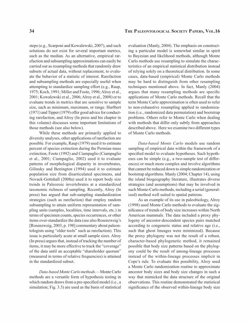
steps (e.g., Scarponi and Kowalewski, 2007), and such solutions do not exist for several important metrics, such as the median. As an alternative, empirical rar-efaction and subsampling approximations can easily be carried out as resampling methods that randomly draw subsets of actual data, without replacement, to evalu-ate the behavior of a statistic of interest. Rarefaction and subsampling methods are especially useful when attempting to standardize sampling effort (e.g., Raup, 1975; Koch, 1991; Miller and Foote, 1996; Alroy et al., 2001; Kowalewski et al., 2006; Alroy et al., 2008) or to evaluate trends in metrics that are sensitive to sample size, such as minimum, maximum, or range. Hurlbert (1971) and Tipper (1979) offer good advice for conduct-ing rarefaction, and Alroy (In press and his chapter in this volume) discusses some important limitations of those methods (see also below).
While these methods are primarily applied to diversity analyses, other applications of rarefaction are possible. For example, Raup (1979) used it to estimate percent of species extinction during the Permian mass extinction, Foote (1992) and Ciampaglio (Ciampaglio et al., 2001; Ciampaglio, 2002) used it to evaluate patterns of morphological disparity in invertebrates, Gilinsky and Benington (1994) used it to estimate population size from disarticulated specimens, and Novack-Gottshall (2008a) used it to report body size trends in Paleozoic invertebrates at a standardized taxonomic richness of sampling. Recently, Alroy (In press) has argued that sub-sampling standardization strategies (such as rarefaction) that employ random subsampling to attain uniform representation of sam-pling units (samples, localities, time intervals, etc.) in terms of specimen counts, species occurrences, or other items over-standardize the data (see also Rosenzweig’s [Rosenzweig, 2003, p. 198] commentary about paleon-tologists using “older tools” such as rarefaction). This issue is particularly acute at small sample sizes. Alroy (In press) argues that, instead of tracking the number of items, it may be more effective to track the “coverage” of the data until an acceptable “shareholder quorum” (measured in terms of relative frequencies) is attained in the standardized subset.
Data-based Monte Carlo methods.—Monte Carlo methods are a versatile form of hypothesis testing in which random draws from a pre-specified model (i.e., a simulation; Fig. 3.3) are used as the basis of statistical
evaluation (Manly, 2004). The emphasis on construct-ing a particular model is somewhat similar in spirit to Bayesian and likelihood methods, although Monte Carlo methods use resampling to simulate the charac-teristics of an empirical statistical distribution instead of relying solely on a theoretical distribution. In some cases, data-based (empirical) Monte Carlo methods may be hard to distinguish from other resampling techniques mentioned above. In fact, Manly (2004) argues that many resampling methods are specific applications of Monte Carlo methods. Recall that the term Monte Carlo approximation is often used to refer to non-exhaustive resampling applied to randomiza-tion (i.e., randomized data permutation) and bootstrap problems. Others refer to Monte Carlo when dealing with methods that differ only subtly from approaches described above. Here we examine two different types of Monte Carlo methods.
Data-based Monte Carlo models use random sampling of empirical data within the framework of a specified model to evaluate hypotheses. Such hypoth-eses can be simple (e.g., a two-sample test of differ-ences) or much more complex and involve algorithms that cannot be reduced down to simple randomization or bootstrap algorithms. Manly (2004; Chapter 14), using the island biogeography literature, illustrates diverse strategies (and assumptions) that may be involved in such Monte-Carlo methods, including a serial (general-ized) method well suited to spatial patterns.
As an example of its use in paleobiology, Alroy (1998) used Monte Carlo methods to evaluate the sig-nificance of trends of body size increases within North American mammals. The data included a proxy phy-logeny of ancestor-descendent species pairs matched according to congeneric status and relative age (i.e., such that ghost lineages were minimized). Because the proxy phylogeny was not the result of a robust, character-based phylogenetic method, it remained possible that body size patterns based on the phylog-eny could be the result of among-lineage processes instead of the within-lineage processes implicit in Cope’s rule. To evaluate this possibility, Alroy used a Monte Carlo randomization routine to approximate ancestor body sizes and body size changes in such a way that mimicked the data structure of the original observations. This routine demonstrated the statistical significance of the observed within-lineage body size
KOWALEWSKI ANd NOVACK-GOTTSHALL—RESAMPLING METHOdS IN PALEONTOLOGy 35
increases because the randomizations were unable to produce the magnitude of size changes observed in the original phylogeny.
Novack-Gottshall and Lanier (2008) used a simi-lar protocol in their analysis of body size evolution in Paleozoic brachiopods. They observed that body size increased within classes and orders, but remained generally unchanged within families. Because family-level phylogenies were not available to test the cause of this, they used Monte Carlo resampling methods to assemble possible ancestor-descendent relationships at random (but consistent with the stratigraphic record) and calculated resampled p-values for various candidate hypotheses that might explain the phylogeny-wide body size trends. In other words, the Monte Carlo protocol allowed them to evaluate how sensitive the possible hypotheses were to various phylogenetic topologies. While not a hypothesis test in the strict sense, the analysis demonstrated that the vast majority of stratigraphically sensible brachiopod phylogenies (83–99%, depending on criteria used to assemble them) would be insufficient to support two of three candidate hypotheses, while ≈74% of such phylogenies were significantly consistent with the hypothesis that body size increases were concentrated during intervals in which new brachiopod families originated.
Although not referred to as “Monte Carlo” by the author, Foote’s (1999) strategy of creating “fake” crinoids by randomly drawing from the set of characters present in the data is another example of the approach. In his simulations, no actual specimens were resampled. Instead, aspects of the data (a list of all character states observed in actual crinoids, in this case) were used to “assemble” artificial crinoids. Foote also constrained his simulations biologically. For example, if a stem was lacking, all stem-related characters were automatically discarded. This is a good example of built-in constraints that make such simulations distinct from simple ran-domizations and bootstrap strategies where all possible data combinations are allowed to occur in resampled data. To compare and contrast morphological radiations of Paleozoic and post-Paleozoic crinoids (note that this is a two-sample problem), Foote used the above protocol to explore two models: (1) the probability of each character state was given by its frequency in the actual data; and (2) the probability of all character states was equal. Each of the two models was simu-lated 1,000 times, with artificial crinoids split into two
samples matching the actual data structure of Paleozoic and post-Paleozoic data sets. The results demonstrated in both cases that real Paleozoic and post-Paleozoic crinoids shared dramatically fewer character-state combinations that would have been possible when “as-sembling” crinoids at random. This specific example represents an intermediate approach between strictly data-based Monte Carlo approaches (where actual data are resampled in some way) and model-based Monte Carlo approaches (where models are used to replicate samples in some way). Foote’s (1999) approach is a mixture of the two—aspects of data are used but not the actual observations.
Model-based Monte Carlo methods.—Model-based (or implicit) Monte Carlo methods differ from the methods discussed above in that they do not use actual observations to create the “resampled” data sets. Instead, “observations” are drawn randomly from some theoretical distribution (Fig. 1). The only information that is often retained is some aspect of the data that is used to define the theoretical distribution. This can be the actual sample structure, the range of values ob-served in the actual data, and so on (arguably, Foote, 1999, discussed above, could be classified here). This theoretical distribution (or model) is then used in the resampling simulation (but the original observations are not resampled).
The trickiest part of the implicit Monte Carlo approach is how to choose and justify the theoretical model from which resampled data are drawn. Three common strategies are worth noting.
1. Theoretical justification.—We may have theo-retical reasons to expect that data should behave in a certain way. As an example, Kowalewski and Rimstidt (2003) assumed that detrital mineral grains would be destroyed by natural geological processes following the simplest type of Weibull function (an exponential decay). Then they used a range of exponential functions (with different “half-lives”) to model age distributions of dated detrital grains, mimicking variable destruction rates for minerals with different chemical and physi-cal durability. The resulting exponential Monte Carlo models performed better than other (uniform, normal) Monte Carlo models. Note that the actual dated grains were not resampled. Instead, an exponential function was used to randomly generate simulated grain ages,
36 the PaleontologIcal socIety PaPers, vol.16
and these random dates were then compiled into sets of samples mimicking the actual structure of the evalu-ated data set. Those Monte Carlo simulations not only suggested that the exponential model performed better than other models but the simulations also successfully simulated the predicted differences in the shapes of age distributions related to different “half-lives” of differ-ent mineral types (see Kowalewski and Rimstidt 2003 for more details).
2. The “extreme model” approach.—In many cases, Monte Carlo models may be useful not because they are justified by some theoretical predictions regarding analyzed systems, but because they can be defined in such a way to simulate an extreme end member of all possible cases. The “random, indepen-dent” end member is a particularly common model, in which researchers evaluate if data can be simulated by a purely stochastic process with all observations acting randomly and independently from one another. Do sto-chastically branching lineages display abrupt changes in diversity (Raup et al., 1973; Gould et al., 1977)? Do drill holes of predatory origin occur randomly across fossil brachiopod species (e.g., Hoffmeister et al., 2004)? Are the gaps observed in Holocene beach ridges of the Colorado River Delta consistent with incomplete sampling of a perfectly complete (i.e., uniform) shell record (Kowalewski et al., 1998)? Such questions can be addressed by invoking Monte Carlo models that mimic data using purely stochastic processes. That is, we build simulations that project random observations onto the actual structure of the empirical data being evaluated. Simulations may be constrained by the sample size and age-ranges of shells observed in each sample for each horizon (Kowalewski et al., 1998). Or, the simulation may be constrained by number of bra-chiopod species, number of brachiopod specimens, and the overall drilling rates (Hoffmeister et al., 2004). Or, the simulation may simply constrain rates of origination and extinction using a priori assumed range of values (Raup et al., 1973; Gould et al., 1977). In either case, the resampling distributions are not produced from data but rather from models constrained by data structure and/or data parameters.
3. Multi-model exploration.—Finally, research-ers may simply decide that they do not know what the right model is and can explore a spectrum of models instead (note that this is similar to bootstrap tests of
multiple hypotheses employed by Wang (2003), as mentioned above). For example, Krause et al. (2010) used an approach similar to the Holocene beach-ridge example above (Kowalewski et al., 1998) to explore a series of different models (uniforrn, uniform with gaps, and exponential) to assess if the observed completeness of age distributions of shells in these deposits can be explained by multiple processes. All these variants of model-based Monte Carlo approaches may be viewed as approaches that are intermediate between empiri-cally constrained resampling methods on one hand, and data-free computer models on the other.
concePtualIZIng resaMPlIng Methods along an “eMPIrIcal
realIty gradIent”
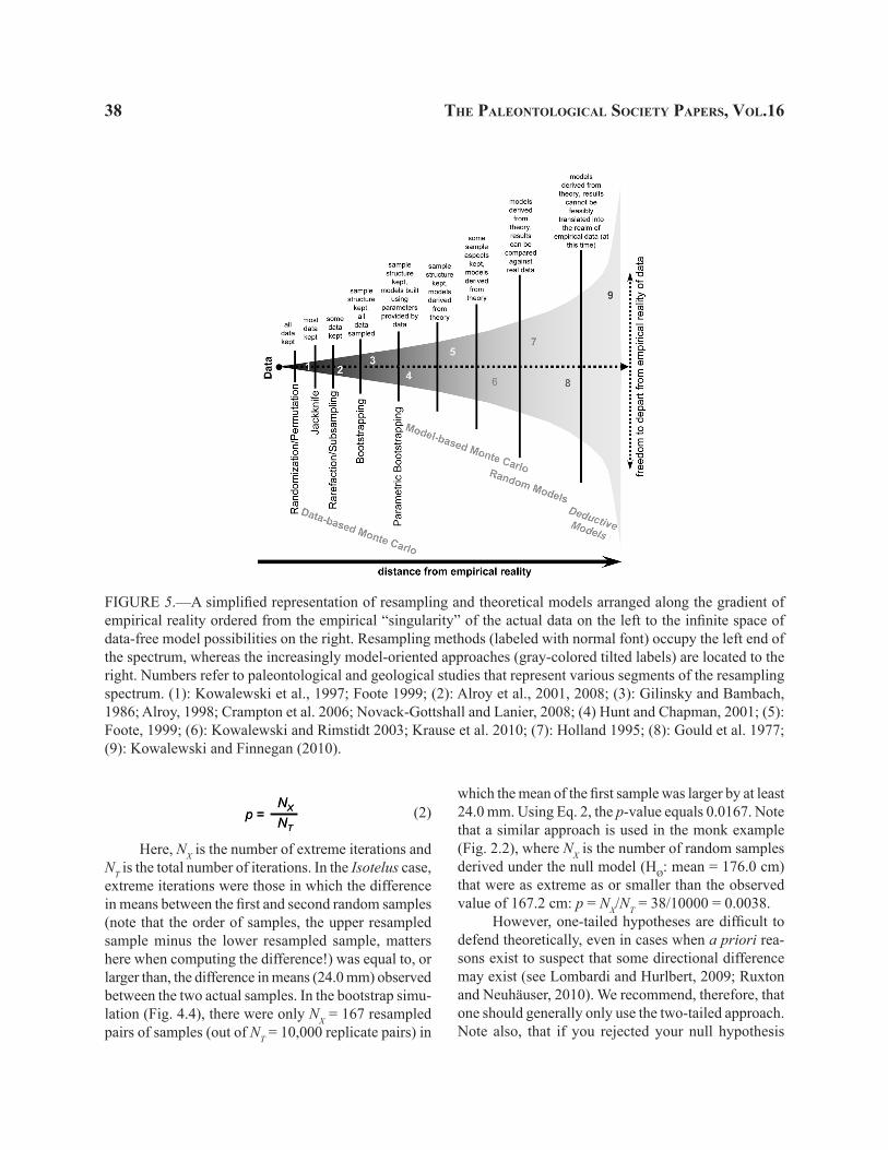
Resampling methods are diverse, conceptually overlapping, and terminologically confusing. However, we can impose some order on this apparent chaos by realizing that they can be arranged along an “empirical reality gradient”, from data-restricted to data-free ap-proaches shown graphically in Fig. 5. On the left we have an empirical “singularity”, a unique predefined value, provided by actual data. Consider that when we apply resampling methods, we are creating a new “re-ality” of resampled statistics. How far we depart from the actual value of our observed data largely depends on the type of resampling methods we employ. Data-based resampling methods are strongly constrained and cannot depart too far from the data. Of those, randomization is the most constrained: all observa-tions are used once in any given iteration. Jackknife, rarefaction, and bootstrap offer increased freedom from actual data because they depart further and further from the constraints of the actual data structure (jackknife alters reality by removing one observation completely, rarefaction can remove more than one observation, and bootstrap can remove multiple observations while du-plicating others). Most of the data-based Monte Carlo methods will also fall in this region of the chart, being constrained by the data (and often being effectively syn-onymous with other data-based resampling methods).
As we move farther away from the “point of singularity” defined by our data, we enter the realm of models that are increasingly less constrained em-pirically. Model-based Monte Carlo methods may still retain some sample information, but the actual values
KOWALEWSKI ANd NOVACK-GOTTSHALL—RESAMPLING METHOdS IN PALEONTOLOGy 37
of observations may be potentially quite different from any values observed in the actual data. A “sample” of ten monks drawn from a normal distribution with mean of 167.2 cm and standard deviation of 15.002 cm can include values that are much smaller or much larger than any of the observed data points. Consider that under the monk-parameterized model, it is possible (if highly improbable) to sample a four-meter tall monk. But a four-meter tall monk could never occur using any data-based resampling methods. Likewise, biologically impossible (e.g., monk-sized) trilobites are indeed impossible when resampling real trilobites. But such impossible trilobites might show up in model-based Monte Carlo models. Thus, parametric bootstrap and model-based Monte Carlo methods are placed further away from the empirical reality of the data than resa-mpling methods sensu stricto.
We can move even farther away into the realm of models that are not tied directly to any data. The classic studies of David Raup and colleagues (Raup et al., 1973; Raup and Gould, 1974; Gould et al., 1977; Raup, 1977; see also Kitchell and MacLeod, 1988), who used stochastic models to generate spindle diagrams (fossil records of clade diversity), is a great example of such an approach. Each spindle diagram was generated by simulating stochastic speciation and extinction events through time. The models were not constrained by real data, but suggested that many groups of organisms have fossil records that can be mimicked by very simple stochastic processes (but see Stanley et al., 1981). Even more useful was the observation that spindle diagrams of some real groups of organisms could not be reproduced by such a simple random process. Such models, while unconstrained by any specific data, can be related back to the reality of empirical patterns. Raup’s (Raup and Michelson, 1965; Raup, 1966, 1967) theoretical morphospace of shell coiling, Holland’s (1995) models of the stratigraphic distributions of fossils, Bambach’s (1983; Bambach et al., 2007; Bush et al., 2007a; Bush et al., In press) and Novack-Gottshall’s (2007) ecospace models, and Novack-Gottshall’s (2006, 2008b) models of ecological community assembly offer other examples of data-free constructs (both qualitative and quantitative) that can then be related back to empirical data.
Finally, at the very end of our spectrum reside deductive models, derived from first principles with minimal constraints imposed by empirical reality. Such
models may produce results difficult to relate directly to any data, although they still can potentially yield indirect insights into various patterns observed in the fossil record. For example, Kowalewski and Finnegan (2010) presented a series of models simulating the be-havior of global marine biodiversity in terms of a few, very basic variables. These data-free results suggest that Phanerozoic diversity could have readily fluctu-ated by orders of magnitude, thus posing an interesting theoretical question why it did not.
Note that this chapter deals primarily with the left part of the diagram, where data-based resampling methods are located. We will now deal with various practical issues of such methods, primarily focusing on the most common resampling methods such as bootstrapping.
PractIcal asPects oF resaMPlIng
Estimating the p-value.—Multiple methods exist
for estimating the p-value, the probability of observing a statistic as large as or more extreme than that observed under a true null hypothesis. But most methods follow the same logic of comparing your observed statistic to the resampling distribution of that statistic predicted under the tested null hypothesis.
Imagine conducting a two-sample bootstrap test of the body sizes of the Isotelus trilobite samples mentioned above. Let us test the one-tailed null hy-pothesis stating that Isotelus from the lower horizon are, on average, at least as big as Isotelus from the upper horizon (HØ µLOWER ≥ µUPPER). Consequently, the alternative one-tailed research hypothesis states that the upper horizon contains larger trilobites (HA µLOWER < µUPPER). The resulting bootstrap distribution of resa-mpled body sizes is presented as a histogram (Fig. 4.4) with the observed mean size difference between the two trilobite samples marked as the rightmost vertical line. It is obvious that few resampled values were as large as or larger than the observed difference.
The most straightforward method for calculating the relevant p-value (and one that is commonly used in paleontology) calculates the p-value as the propor-tion of resampled iterations (obtained under the null hypothesis), which are at least as different from the parameter of interest (e.g., mean) as is the observed statistic. The value of p is then given by:
38 the PaleontologIcal socIety PaPers, vol.16
(2)
Here, NX is the number of extreme iterations and NT is the total number of iterations. In the Isotelus case, extreme iterations were those in which the difference in means between the first and second random samples (note that the order of samples, the upper resampled sample minus the lower resampled sample, matters here when computing the difference!) was equal to, or larger than, the difference in means (24.0 mm) observed between the two actual samples. In the bootstrap simu-lation (Fig. 4.4), there were only NX = 167 resampled pairs of samples (out of NT = 10,000 replicate pairs) in
Eq. 2 p =NX
NTEq. 2 p =
NX
NT
which the mean of the first sample was larger by at least 24.0 mm. Using Eq. 2, the p-value equals 0.0167. Note that a similar approach is used in the monk example (Fig. 2.2), where NX is the number of random samples derived under the null model (HØ: mean = 176.0 cm) that were as extreme as or smaller than the observed value of 167.2 cm: p = NX/NT = 38/10000 = 0.0038.
However, one-tailed hypotheses are difficult to defend theoretically, even in cases when a priori rea-sons exist to suspect that some directional difference may exist (see Lombardi and Hurlbert, 2009; Ruxton and Neuhäuser, 2010). We recommend, therefore, that one should generally only use the two-tailed approach. Note also, that if you rejected your null hypothesis
FIGURE 5.—A simplified representation of resampling and theoretical models arranged along the gradient of empirical reality ordered from the empirical “singularity” of the actual data on the left to the infinite space of data-free model possibilities on the right. Resampling methods (labeled with normal font) occupy the left end of the spectrum, whereas the increasingly model-oriented approaches (gray-colored tilted labels) are located to the right. Numbers refer to paleontological and geological studies that represent various segments of the resampling spectrum. (1): Kowalewski et al., 1997; Foote 1999; (2): Alroy et al., 2001, 2008; (3): Gilinsky and Bambach, 1986; Alroy, 1998; Crampton et al. 2006; Novack-Gottshall and Lanier, 2008; (4) Hunt and Chapman, 2001; (5): Foote, 1999; (6): Kowalewski and Rimstidt 2003; Krause et al. 2010; (7): Holland 1995; (8): Gould et al. 1977; (9): Kowalewski and Finnegan (2010).
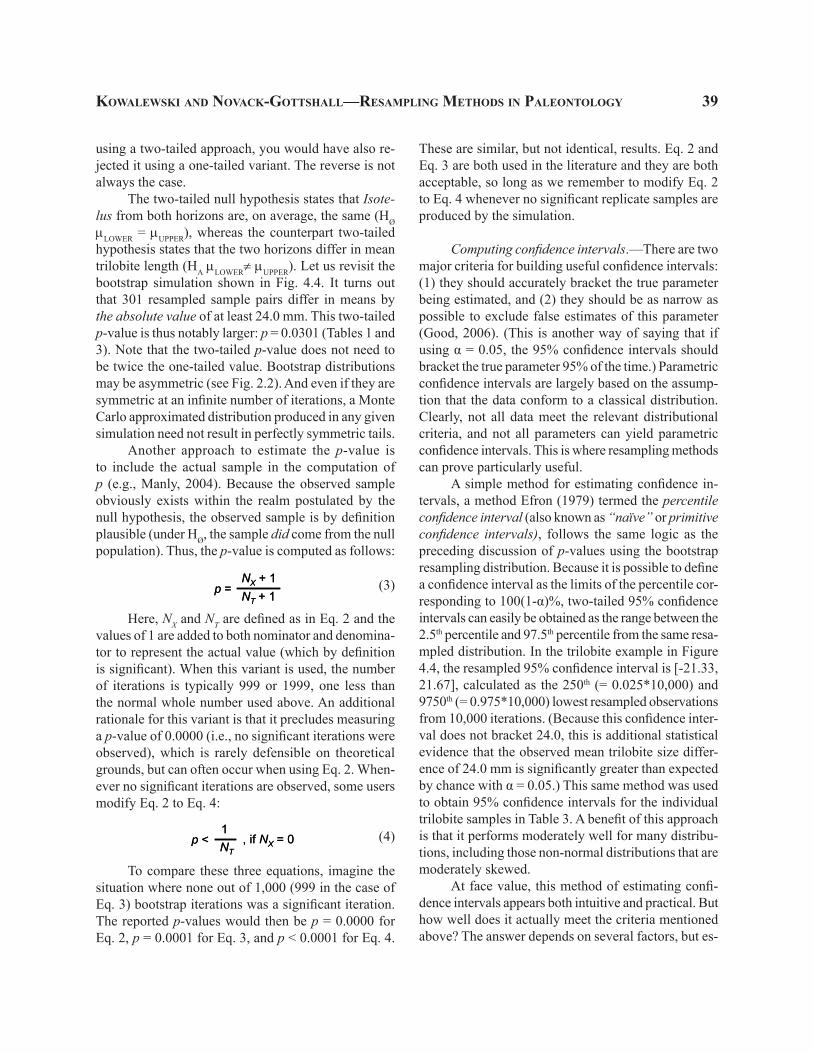
KOWALEWSKI ANd NOVACK-GOTTSHALL—RESAMPLING METHOdS IN PALEONTOLOGy 39
using a two-tailed approach, you would have also re-jected it using a one-tailed variant. The reverse is not always the case.
The two-tailed null hypothesis states that Isote-lus from both horizons are, on average, the same (HØ µLOWER = µUPPER), whereas the counterpart two-tailed hypothesis states that the two horizons differ in mean trilobite length (HA µLOWER≠ µUPPER). Let us revisit the bootstrap simulation shown in Fig. 4.4. It turns out that 301 resampled sample pairs differ in means by the absolute value of at least 24.0 mm. This two-tailed p-value is thus notably larger: p = 0.0301 (Tables 1 and 3). Note that the two-tailed p-value does not need to be twice the one-tailed value. Bootstrap distributions may be asymmetric (see Fig. 2.2). And even if they are symmetric at an infinite number of iterations, a Monte Carlo approximated distribution produced in any given simulation need not result in perfectly symmetric tails.
Another approach to estimate the p-value is to include the actual sample in the computation of p (e.g., Manly, 2004). Because the observed sample obviously exists within the realm postulated by the null hypothesis, the observed sample is by definition plausible (under HØ, the sample did come from the null population). Thus, the p-value is computed as follows:
(3)
Here, NX and NT are defined as in Eq. 2 and the values of 1 are added to both nominator and denomina-tor to represent the actual value (which by definition is significant). When this variant is used, the number of iterations is typically 999 or 1999, one less than the normal whole number used above. An additional rationale for this variant is that it precludes measuring a p-value of 0.0000 (i.e., no significant iterations were observed), which is rarely defensible on theoretical grounds, but can often occur when using Eq. 2. When-ever no significant iterations are observed, some users modify Eq. 2 to Eq. 4:
(4)
To compare these three equations, imagine the situation where none out of 1,000 (999 in the case of Eq. 3) bootstrap iterations was a significant iteration. The reported p-values would then be p = 0.0000 for Eq. 2, p = 0.0001 for Eq. 3, and p < 0.0001 for Eq. 4.
Eq. 3 p =NX + 1NT + 1Eq. 3 p =NX + 1NT + 1
Eq. 4 , if NX = 0p <1NT
Eq. 4 , if NX = 0p <1NT
These are similar, but not identical, results. Eq. 2 and Eq. 3 are both used in the literature and they are both acceptable, so long as we remember to modify Eq. 2 to Eq. 4 whenever no significant replicate samples are produced by the simulation.
Computing confidence intervals.—There are two major criteria for building useful confidence intervals: (1) they should accurately bracket the true parameter being estimated, and (2) they should be as narrow as possible to exclude false estimates of this parameter (Good, 2006). (This is another way of saying that if using α = 0.05, the 95% confidence intervals should bracket the true parameter 95% of the time.) Parametric confidence intervals are largely based on the assump-tion that the data conform to a classical distribution. Clearly, not all data meet the relevant distributional criteria, and not all parameters can yield parametric confidence intervals. This is where resampling methods can prove particularly useful.
A simple method for estimating confidence in-tervals, a method Efron (1979) termed the percentile confidence interval (also known as “naïve” or primitive confidence intervals), follows the same logic as the preceding discussion of p-values using the bootstrap resampling distribution. Because it is possible to define a confidence interval as the limits of the percentile cor-responding to 100(1-α)%, two-tailed 95% confidence intervals can easily be obtained as the range between the 2.5th percentile and 97.5th percentile from the same resa-mpled distribution. In the trilobite example in Figure 4.4, the resampled 95% confidence interval is [-21.33, 21.67], calculated as the 250th (= 0.025*10,000) and 9750th (= 0.975*10,000) lowest resampled observations from 10,000 iterations. (Because this confidence inter-val does not bracket 24.0, this is additional statistical evidence that the observed mean trilobite size differ-ence of 24.0 mm is significantly greater than expected by chance with α = 0.05.) This same method was used to obtain 95% confidence intervals for the individual trilobite samples in Table 3. A benefit of this approach is that it performs moderately well for many distribu-tions, including those non-normal distributions that are moderately skewed.
At face value, this method of estimating confi-dence intervals appears both intuitive and practical. But how well does it actually meet the criteria mentioned above? The answer depends on several factors, but es-
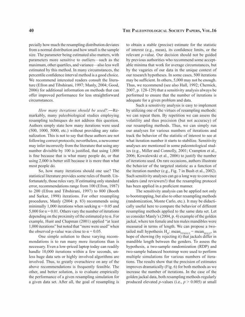
40 the PaleontologIcal socIety PaPers, vol.16
pecially how much the resampling distribution deviates from a normal distribution and how small is the sample size. The parameter being estimated also matters, with parameters more sensitive to outliers—such as the maximum, other quartiles, and variance—also less well estimated by this method. In many circumstances, the percentile confidence interval method is a good choice. We recommend interested readers consult the litera-ture (Efron and Tibshirani, 1997; Manly, 2004; Good, 2006) for additional information on methods that can offer improved performance for less straightforward circumstances.
How many iterations should be used?.—Re-markably, many paleobiological studies employing resampling techniques do not address this question. Authors simply state how many iterations were used (500, 1000, 5000, etc.) without providing any ratio-nalization. This is not to say that these authors are not following correct protocols; nevertheless, a newcomer may infer incorrectly from the literature that using any number divisible by 100 is justified, that using 1,000 is fine because that is what many people do, or that using 2,000 is better still because it is more than what most people do.
So, how many iterations should one use? The statistical literature provides some rules of thumb. Un-fortunately, those rules vary. If estimating only standard error, recommendations range from 100 (Efron, 1987) to 200 (Efron and Tibshirani, 1997) to 800 (Booth and Sarkar, 1998) iterations. For other resampling procedures, Manly (2004: p. 83) recommends using minimally 1,000 iterations when seeking α = 0.05 and 5,000 for α = 0.01. Others vary the number of iterations depending on the proximity of the estimated p to α. For example, Hunt and Chapman (2001) applied “at least 1,000 iterations” but noted that “more were used” when the observed p-value was close to α = 0.05.
One simple solution to these varying recom-mendations is to run many more iterations than is necessary. Even a low-priced laptop today can readily handle 10,000 iterations within a few seconds, un-less huge data sets or highly involved algorithms are involved. Thus, to greatly overachieve on any of the above recommendations is frequently feasible. The other, and better solution, is to evaluate empirically the performance of a given resampling simulation for a given data set. After all, the goal of resampling is
to obtain a stable (precise) estimate for the statistic of interest (e.g., mean), its confidence limits, or the relevant p-value. Our decision should not be guided by previous authorities who recommend some accept-able minima that work for average circumstances, but by the vagaries of our data in the unique context of our research hypotheses. In some cases, 500 iterations may be sufficient. In others, 5,000 may not be enough. Thus, we recommend (see also Hall, 1992; Chernick, 2007, p. 128-129) that a sensitivity analysis always be performed to ensure that the number of iterations is adequate for a given problem and data.
Such a sensitivity analysis is easy to implement by utilizing one of the virtues of resampling methods: we can repeat them. By repetition we can assess the volatility and thus precision (but not accuracy) of our resampling methods. Thus, we can simply run our analyses for various numbers of iterations and track the behavior of the statistic of interest to see at what iteration number it starts to stabilize. Sensitivity analyses are mentioned in some paleontological stud-ies (e.g., Miller and Connolly, 2001; Crampton et al., 2006; Kowalewski et al., 2006) to justify the number of iterations used. On rare occasions, authors illustrate the behavior of the targeted statistic as a function of the iteration number (e.g., Fig. 7 in Bush et al., 2002). Such sensitivity analyses can go a long way to convince readers (and reviewers!) that the resampling protocol has been applied in a proficient manner.
The sensitivity analysis can be applied not only to bootstrapping, but also to other resampling methods (randomization, Monte Carlo, etc.). It may be didacti-cally useful here to compare the behavior of different resampling methods applied to the same data set. Let us consider Manly’s (2004, p. 4) example of the golden jackal, where ten female and ten males mandibles were measured in terms of length. We can propose a two-tailed null hypothesis HØ: meanFEMALE = meanMALE, in hope of showing (by rejecting it) that jackals differ in mandible length between the genders. To assess the hypothesis, a two-sample randomization (RDP) and two-sample balanced bootstrap were used to perform multiple simulations for various numbers of itera-tions. The results show that the precision of estimates improves dramatically (Fig. 6) for both methods as we increase the number of iterations. In the case of the golden jackal data, both resampling methods regularly produced elevated p-values (i.e., p > 0.005) at small
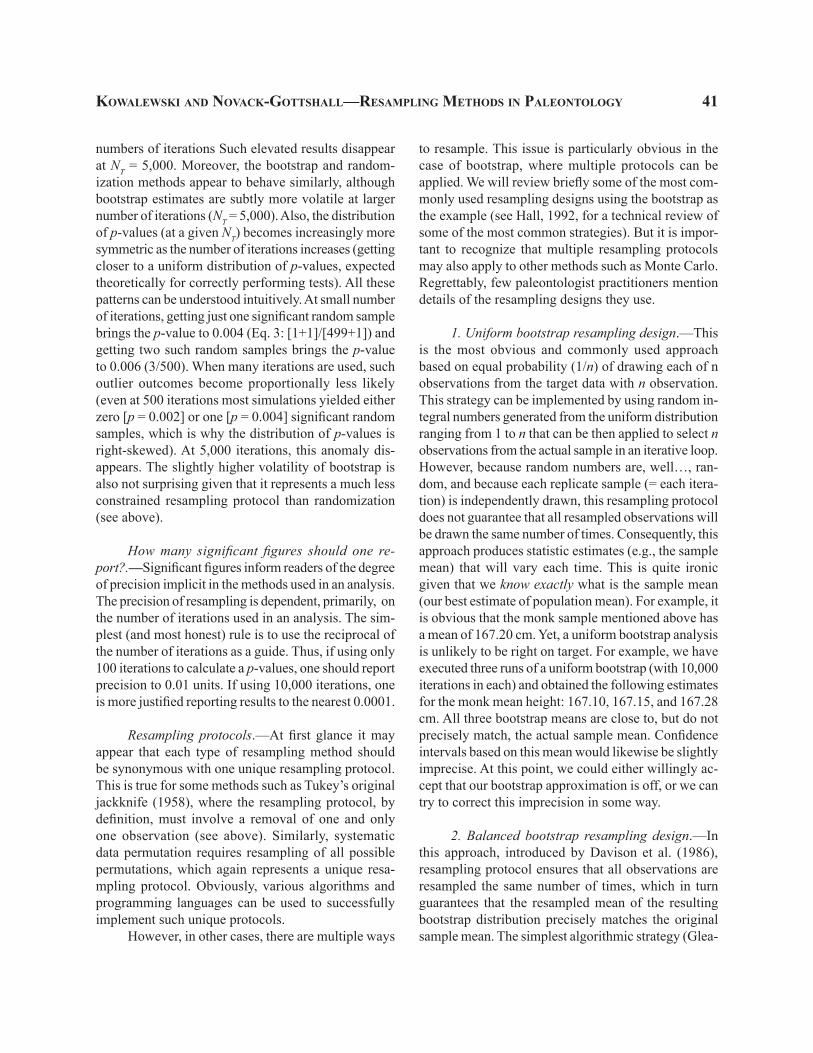
KOWALEWSKI ANd NOVACK-GOTTSHALL—RESAMPLING METHOdS IN PALEONTOLOGy 41
numbers of iterations Such elevated results disappear at NT = 5,000. Moreover, the bootstrap and random-ization methods appear to behave similarly, although bootstrap estimates are subtly more volatile at larger number of iterations (NT = 5,000). Also, the distribution of p-values (at a given NT) becomes increasingly more symmetric as the number of iterations increases (getting closer to a uniform distribution of p-values, expected theoretically for correctly performing tests). All these patterns can be understood intuitively. At small number of iterations, getting just one significant random sample brings the p-value to 0.004 (Eq. 3: [1+1]/[499+1]) and getting two such random samples brings the p-value to 0.006 (3/500). When many iterations are used, such outlier outcomes become proportionally less likely (even at 500 iterations most simulations yielded either zero [p = 0.002] or one [p = 0.004] significant random samples, which is why the distribution of p-values is right-skewed). At 5,000 iterations, this anomaly dis-appears. The slightly higher volatility of bootstrap is also not surprising given that it represents a much less constrained resampling protocol than randomization (see above).
How many significant figures should one re-port?.—Significant figures inform readers of the degree of precision implicit in the methods used in an analysis. The precision of resampling is dependent, primarily, on the number of iterations used in an analysis. The sim-plest (and most honest) rule is to use the reciprocal of the number of iterations as a guide. Thus, if using only 100 iterations to calculate a p-values, one should report precision to 0.01 units. If using 10,000 iterations, one is more justified reporting results to the nearest 0.0001.
Resampling protocols.—At first glance it may appear that each type of resampling method should be synonymous with one unique resampling protocol. This is true for some methods such as Tukey’s original jackknife (1958), where the resampling protocol, by definition, must involve a removal of one and only one observation (see above). Similarly, systematic data permutation requires resampling of all possible permutations, which again represents a unique resa-mpling protocol. Obviously, various algorithms and programming languages can be used to successfully implement such unique protocols.
However, in other cases, there are multiple ways
to resample. This issue is particularly obvious in the case of bootstrap, where multiple protocols can be applied. We will review briefly some of the most com-monly used resampling designs using the bootstrap as the example (see Hall, 1992, for a technical review of some of the most common strategies). But it is impor-tant to recognize that multiple resampling protocols may also apply to other methods such as Monte Carlo. Regrettably, few paleontologist practitioners mention details of the resampling designs they use.
1. Uniform bootstrap resampling design.—This is the most obvious and commonly used approach based on equal probability (1/n) of drawing each of n observations from the target data with n observation. This strategy can be implemented by using random in-tegral numbers generated from the uniform distribution ranging from 1 to n that can be then applied to select n observations from the actual sample in an iterative loop. However, because random numbers are, well…, ran-dom, and because each replicate sample (= each itera-tion) is independently drawn, this resampling protocol does not guarantee that all resampled observations will be drawn the same number of times. Consequently, this approach produces statistic estimates (e.g., the sample mean) that will vary each time. This is quite ironic given that we know exactly what is the sample mean (our best estimate of population mean). For example, it is obvious that the monk sample mentioned above has a mean of 167.20 cm. Yet, a uniform bootstrap analysis is unlikely to be right on target. For example, we have executed three runs of a uniform bootstrap (with 10,000 iterations in each) and obtained the following estimates for the monk mean height: 167.10, 167.15, and 167.28 cm. All three bootstrap means are close to, but do not precisely match, the actual sample mean. Confidence intervals based on this mean would likewise be slightly imprecise. At this point, we could either willingly ac-cept that our bootstrap approximation is off, or we can try to correct this imprecision in some way.
2. Balanced bootstrap resampling design.—In this approach, introduced by Davison et al. (1986), resampling protocol ensures that all observations are resampled the same number of times, which in turn guarantees that the resampled mean of the resulting bootstrap distribution precisely matches the original sample mean. The simplest algorithmic strategy (Glea-
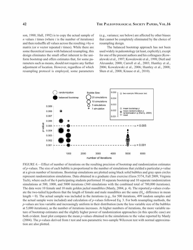
42 the PaleontologIcal socIety PaPers, vol.16
FIGURE 6.—Effect of number of iterations on the resulting precision of bootstrap and randomization estimates of p-values. The size of each bubble is proportional to the number of simulations that yielded a particular p-value at a given number of iterations. Bootstrap simulations are plotted using black solid bubbles and gray open circles represent randomization simulations. Data obtained in a graduate class exercise (Geos 5374, Fall 2009, Virginia Tech), where each of the 6 participating students performed 10 separate bootstrap and 10 separate randomization simulations at 500, 1000, and 5000 iterations (360 simulations with the combined total of 780,000 iterations). The data were 10 female and 10 male golden jackal mandibles (Manly, 2004, p. 4). The reported p-values evalu-ate the two-tailed hypothesis that the length of female and male mandibles are the same (HØ: difference in mean length = 0). The actual sample was included in the iterations (e.g., for 500 iterations, 499 random samples and the actual sample were included) and calculation of p-values followed Eq. 3. For both resampling methods, the p-values are less variable and increasingly uniform in their distribution (note the less variable size of the bubbles at 5,000 iterations), as the number of iterations increases. At higher numbers of iterations, the more variable na-ture of bootstrap estimates and the slightly higher power of randomization approaches (in this specific case) are both evident. Inset plot compares the mean p-values obtained in the simulations to the value reported by Manly (2004). The p-values derived from t test and non-parametric two-sample Wilcoxon test with normal approxima-tion are also plotted.
son, 1988; Hall, 1992) is to copy the actual sample of n values i times (where i is the number of iterations) and then reshuffle all values across the resulting i-by-n matrix (or n vector repeated i times). While there are some theoretical issues with balanced resampling, this design eliminates the small offset inherent to the uni-form bootstrap and offers estimates that, for some pa-rameters such as means, should not require any further adjustment of location. However, regardless of which resampling protocol is employed, some parameters
(e.g., variance; see below) are affected by other biases that cannot be completely eliminated by the choice of resampling design.
The balanced bootstrap approach has not been used widely in paleontology (at least, explicitly), except for one of the present authors and his colleagues (Kow-alewski et al., 1997; Kowalewski et al., 1998; Dietl and Alexander, 2000; Carroll et al., 2003; Huntley et al., 2006; Kowalewski et al., 2006; Huntley et al., 2008; Shen et al., 2008; Krause et al., 2010).
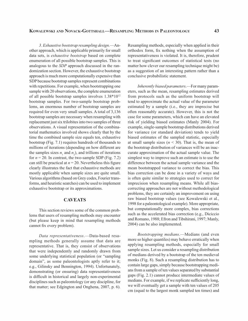
KOWALEWSKI ANd NOVACK-GOTTSHALL—RESAMPLING METHOdS IN PALEONTOLOGy 43
3. Exhaustive bootstrap resampling design.—An-other approach, which is applicable primarily for small data sets, is exhaustive bootstrap based on complete enumeration of all possible bootstrap samples. This is analogous to the SDP approach discussed in the ran-domization section. However, the exhaustive bootstrap approach is much more computationally expensive than SDP because bootstrap samples represent combinations with repetitions. For example, when bootstrapping one sample with 20 observations, the complete enumeration of all possible bootstrap samples involves 1.38*1012 bootstrap samples. For two-sample bootstrap prob-lems, an enormous number of bootstrap samples are required for even very small samples. A total of 3,136 bootstrap samples are necessary when resampling with replacement just six trilobites into two samples of three observations. A visual representation of the combina-torial mathematics involved shows clearly that by the time the combined sample size equals ten, exhaustive bootstrap (Fig. 7.1) requires hundreds of thousands to millions of iterations (depending on how different are the samples sizes n1 and n2), and trillions of iterations for n = 20. In contrast, the two-sample SDP (Fig. 7.2) can still be practical at n = 20. Nevertheless this figure clearly illustrates the fact that exhaustive methods are mostly applicable when sample sizes are quite small. Various algorithms (based on Grey codes, Fourier trans-forms, and heuristic searches) can be used to implement exhaustive bootstrap or its approximations.
caveats
This section reviews some of the common prob-lems that users of resampling methods may encounter (but please keep in mind that resampling methods cannot fix every problem).
Data representativeness.—Data-based resa-mpling methods generally assume that data are representative. That is, they consist of observations that were independently and randomly drawn from some underlying statistical population (or “sampling domain”, as some paleontologists aptly refer to it; e.g., Gilinsky and Bennington, 1994). Unfortunately, demonstrating (or ensuring) data representativeness is difficult in historical and largely non-experimental disciplines such as paleontology (or any discipline, for that matter; see Edgington and Onghena, 2007, p. 6).
Resampling methods, especially when applied in their orthodox form, fix nothing when the assumption of representativeness is violated. It is, therefore, prudent to treat significant outcomes of statistical tests (no matter how clever our resampling technique might be) as a suggestion of an interesting pattern rather than a conclusive probabilistic statement.
Inherently biased parameters.—For many param-eters, such as the mean, resampling estimates derived from protocols such as the uniform bootstrap will tend to approximate the actual value of the parameter estimated by a sample (i.e., they are imprecise but often reasonably accurate). However, this is not the case for some parameters, which can have an elevated risk of yielding biased estimates (Manly 2004). For example, single-sample bootstrap distributions derived for variance (or standard deviation) tends to yield biased estimates of the sampled statistic, especially at small sample sizes (n < 30). That is, the mean of the bootstrap distribution of variances will be an inac-curate approximation of the actual sample value. The simplest way to improve such an estimate is to use the difference between the actual sample variance and the mean bootstrapped variance to correct the bias. This bias correction can be done in a variety of ways and is often quite similar to strategies used to correct for imprecision when resampling means. While all bias-correcting approaches are not without methodological problems, they are certainly an improvement on using raw biased bootstrap values (see Kowalewski et al., 1998 for a paleontological example). More appropriate, but computationally more complex, bias corrections such as the accelerated bias correction (e.g., Diciccio and Romano, 1988; Efron and Tibshirani, 1997; Manly, 2004) can be also implemented.
Bootstrapping medians.—Medians (and even more so higher quantiles) may behave erratically when applying resampling methods, especially for small sample sizes. Let us consider a resampling distribution of medians derived by a bootstrap of the ten medieval monks (Fig. 8). Such a resampling distribution has to contain large gaps, simply because bootstrapping medi-ans from a sample of ten values separated by substantial gaps (Fig. 2.1) cannot produce intermediate values of medians. For example, if we replicate sufficiently long, we will eventually get a sample with ten values of 205 cm (equal to the largest monk sampled ten times) and
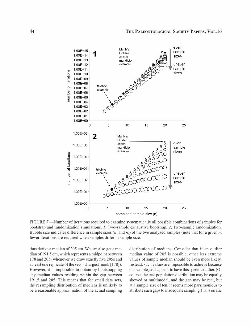
44 the PaleontologIcal socIety PaPers, vol.16
thus derive a median of 205 cm. We can also get a me-dian of 191.5 cm, which represents a midpoint between 178 and 205 (whenever we draw exactly five 205s and at least one replicate of the second largest monk [178]). However, it is impossible to obtain by bootstrapping any median values residing within the gap between 191.5 and 205. This means that for small data sets, the resampling distribution of medians is unlikely to be a reasonable approximation of the actual sampling
distribution of medians. Consider that if an outlier median value of 205 is possible, other less extreme values of sample median should be even more likely. Instead, such values are impossible to achieve because our sample just happens to have this specific outlier. (Of course, the true population distribution may be equally skewed or multimodal, and the gap may be real, but at a sample size of ten, it seems more parsimonious to attribute such gaps to inadequate sampling.) This erratic
FIGURE 7.—Number of iterations required to examine systematically all possible combinations of samples for bootstrap and randomization simulations. 1, Two-sample exhaustive bootstrap. 2, Two-sample randomization. Bubble size indicates difference in sample sizes (n1 and n2) of the two analyzed samples (note that for a given n, fewer iterations are required when samples differ in sample size.
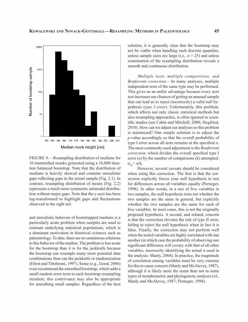
KOWALEWSKI ANd NOVACK-GOTTSHALL—RESAMPLING METHOdS IN PALEONTOLOGy 45
and unrealistic behavior of bootstrapped medians is a particularly acute problem when samples are used to estimate underlying statistical populations, which is a dominant motivation in historical sciences such as paleontology. To date, there are no unanimous solutions to this behavior of the median. The problem is less acute for the bootstrap than it is for the jackknife because the bootstrap can resample many more potential data combinations than can the jackknife or randomization (Efron and Tibshirani, 1997). Some (e.g., Good, 2006) even recommend the smoothed bootstrap, which adds a small random error term to each bootstrap resampling iteration; this contrivance may also be appropriate for smoothing small samples. Regardless of the best
solution, it is generally clear that the bootstrap may not be viable when handling such discrete quantiles, unless sample sizes are large (i.e., n > 25) and unless examination of the resampling distribution reveals a smooth and continuous distribution.
Multiple tests, multiple comparisons, and Bonferroni correction.—In many analyses, multiple independent tests of the same type may be performed. This gives us an unfair advantage because every next test increases our chances of getting an unusual sample that can lead us to reject (incorrectly) a valid null hy-pothesis (type I error). Unfortunately, this problem, which affects not only classic statistical methods but also resampling approaches, is often ignored in scien-tific studies (see Cabin and Mitchell, 2000; Siegfried, 2010). How can we adjust our analyses so this problem is minimized? One simple solution is to adjust the p-value accordingly so that the overall probability of type I error across all tests remains at the specified α. The most commonly used adjustment is the Bonferroni correction, which divides the overall specified type I error (α) by the number of comparisons (k) attempted: αB = α/k.
However, several caveats should be considered when using this correction. The first is that the cor-rection explicitly forces your null hypothesis to test for differences across all variables equally (Perneger, 1998). In other words, in a test of five variables in two samples, the null hypothesis tests not whether the two samples are the same in general, but explicitly whether the two samples are the same for each of five variables. In most cases, this is not the originally proposed hypothesis. A second, and related, concern is that the correction elevates the risk of type II error, failing to reject the null hypothesis when in fact it is false. Finally, the correction may not perform well when the tested variables are highly correlated with one another (in which case the probability of observing one significant difference will covary with that of all other variables, incorrectly identifying the actual α used in the analysis: Manly, 2004). In practice, the magnitude of correlation among variables must be very extreme for this to cause concern (Manly and McAlevey, 1987), although it is likely more the norm than not in some types of morphometric and phylogenetic analyses (cf., Manly and McAlevey, 1987; Perneger, 1998).
FIGURE 8.—Resampling distribution of medians for 10 mummified monks generated using a 10,000 itera-tion balanced bootstrap. Note that the distribution of medians is heavily skewed and contains unrealistic gaps reflecting gaps in the actual sample (Fig. 2.1). In contrast, resampling distribution of means (Fig. 2.2) represents a much more symmetric unimodal distribu-tion without major gaps. Note that the y-axis has been log-transformed to highlight gaps and fluctuations observed in the right tail.
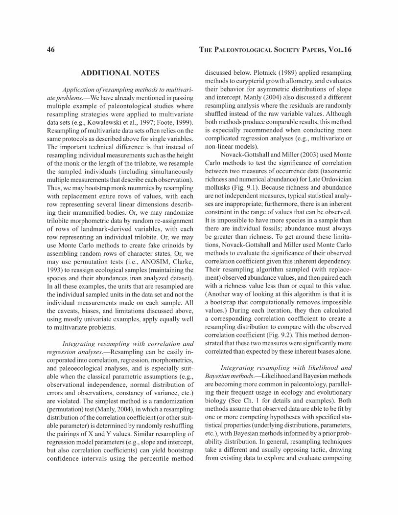
46 the PaleontologIcal socIety PaPers, vol.16
addItIonal notes
Application of resampling methods to multivari-ate problems.—We have already mentioned in passing multiple example of paleontological studies where resampling strategies were applied to multivariate data sets (e.g., Kowalewski et al., 1997; Foote, 1999). Resampling of multivariate data sets often relies on the same protocols as described above for single variables. The important technical difference is that instead of resampling individual measurements such as the height of the monk or the length of the trilobite, we resample the sampled individuals (including simultaneously multiple measurements that describe each observation). Thus, we may bootstrap monk mummies by resampling with replacement entire rows of values, with each row representing several linear dimensions describ-ing their mummified bodies. Or, we may randomize trilobite morphometric data by random re-assignment of rows of landmark-derived variables, with each row representing an individual trilobite. Or, we may use Monte Carlo methods to create fake crinoids by assembling random rows of character states. Or, we may use permutation tests (i.e., ANOSIM, Clarke, 1993) to reassign ecological samples (maintaining the species and their abundances inan analyzed dataset). In all these examples, the units that are resampled are the individual sampled units in the data set and not the individual measurements made on each sample. All the caveats, biases, and limitations discussed above, using mostly univariate examples, apply equally well to multivariate problems.
Integrating resampling with correlation and regression analyses.—Resampling can be easily in-corporated into correlation, regression, morphometrics, and paleoecological analyses, and is especially suit-able when the classical parametric assumptions (e.g., observational independence, normal distribution of errors and observations, constancy of variance, etc.) are violated. The simplest method is a randomization (permutation) test (Manly, 2004), in which a resampling distribution of the correlation coefficient (or other suit-able parameter) is determined by randomly reshuffling the pairings of X and Y values. Similar resampling of regression model parameters (e.g., slope and intercept, but also correlation coefficients) can yield bootstrap confidence intervals using the percentile method
discussed below. Plotnick (1989) applied resampling methods to eurypterid growth allometry, and evaluates their behavior for asymmetric distributions of slope and intercept. Manly (2004) also discussed a different resampling analysis where the residuals are randomly shuffled instead of the raw variable values. Although both methods produce comparable results, this method is especially recommended when conducting more complicated regression analyses (e.g., multivariate or non-linear models).
Novack-Gottshall and Miller (2003) used Monte Carlo methods to test the significance of correlation between two measures of occurrence data (taxonomic richness and numerical abundance) for Late Ordovician mollusks (Fig. 9.1). Because richness and abundance are not independent measures, typical statistical analy-ses are inappropriate; furthermore, there is an inherent constraint in the range of values that can be observed. It is impossible to have more species in a sample than there are individual fossils; abundance must always be greater than richness. To get around these limita-tions, Novack-Gottshall and Miller used Monte Carlo methods to evaluate the significance of their observed correlation coefficient given this inherent dependency. Their resampling algorithm sampled (with replace-ment) observed abundance values, and then paired each with a richness value less than or equal to this value. (Another way of looking at this algorithm is that it is a bootstrap that computationally removes impossible values.) During each iteration, they then calculated a corresponding correlation coefficient to create a resampling distribution to compare with the observed correlation coefficient (Fig. 9.2). This method demon-strated that these two measures were significantly more correlated than expected by these inherent biases alone.
Integrating resampling with likelihood and Bayesian methods.—Likelihood and Bayesian methods are becoming more common in paleontology, parallel-ing their frequent usage in ecology and evolutionary biology (See Ch. 1 for details and examples). Both methods assume that observed data are able to be fit by one or more competing hypotheses with specified sta-tistical properties (underlying distributions, parameters, etc.), with Bayesian methods informed by a prior prob-ability distribution. In general, resampling techniques take a different and usually opposing tactic, drawing from existing data to explore and evaluate competing
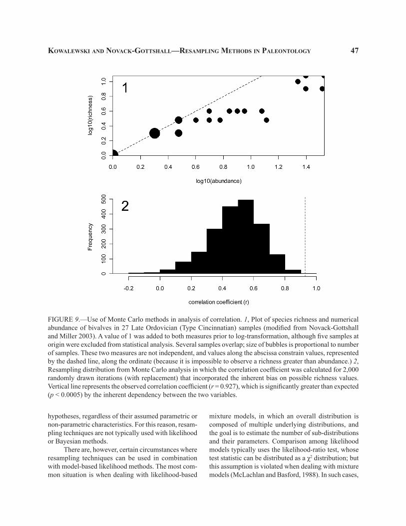
KOWALEWSKI ANd NOVACK-GOTTSHALL—RESAMPLING METHOdS IN PALEONTOLOGy 47
hypotheses, regardless of their assumed parametric or non-parametric characteristics. For this reason, resam-pling techniques are not typically used with likelihood or Bayesian methods.
There are, however, certain circumstances where resampling techniques can be used in combination with model-based likelihood methods. The most com-mon situation is when dealing with likelihood-based
mixture models, in which an overall distribution is composed of multiple underlying distributions, and the goal is to estimate the number of sub-distributions and their parameters. Comparison among likelihood models typically uses the likelihood-ratio test, whose test statistic can be distributed as a χ2 distribution; but this assumption is violated when dealing with mixture models (McLachlan and Basford, 1988). In such cases,
FIGURE 9.—Use of Monte Carlo methods in analysis of correlation. 1, Plot of species richness and numerical abundance of bivalves in 27 Late Ordovician (Type Cincinnatian) samples (modified from Novack-Gottshall and Miller 2003). A value of 1 was added to both measures prior to log-transformation, although five samples at origin were excluded from statistical analysis. Several samples overlap; size of bubbles is proportional to number of samples. These two measures are not independent, and values along the abscissa constrain values, represented by the dashed line, along the ordinate (because it is impossible to observe a richness greater than abundance.) 2, Resampling distribution from Monte Carlo analysis in which the correlation coefficient was calculated for 2,000 randomly drawn iterations (with replacement) that incorporated the inherent bias on possible richness values. Vertical line represents the observed correlation coefficient (r = 0.927), which is significantly greater than expected (p < 0.0005) by the inherent dependency between the two variables.
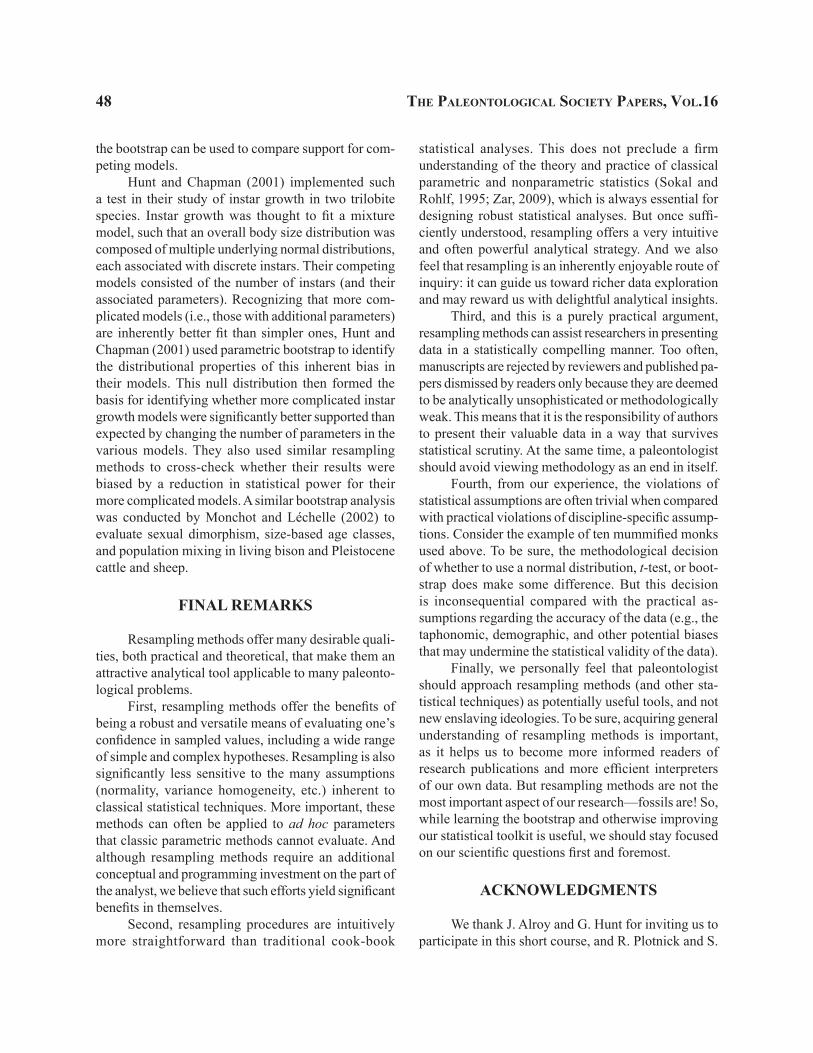
48 the PaleontologIcal socIety PaPers, vol.16
the bootstrap can be used to compare support for com-peting models.
Hunt and Chapman (2001) implemented such a test in their study of instar growth in two trilobite species. Instar growth was thought to fit a mixture model, such that an overall body size distribution was composed of multiple underlying normal distributions, each associated with discrete instars. Their competing models consisted of the number of instars (and their associated parameters). Recognizing that more com-plicated models (i.e., those with additional parameters) are inherently better fit than simpler ones, Hunt and Chapman (2001) used parametric bootstrap to identify the distributional properties of this inherent bias in their models. This null distribution then formed the basis for identifying whether more complicated instar growth models were significantly better supported than expected by changing the number of parameters in the various models. They also used similar resampling methods to cross-check whether their results were biased by a reduction in statistical power for their more complicated models. A similar bootstrap analysis was conducted by Monchot and Léchelle (2002) to evaluate sexual dimorphism, size-based age classes, and population mixing in living bison and Pleistocene cattle and sheep.
FINAL REMARKS
Resampling methods offer many desirable quali-ties, both practical and theoretical, that make them an attractive analytical tool applicable to many paleonto-logical problems.
First, resampling methods offer the benefits of being a robust and versatile means of evaluating one’s confidence in sampled values, including a wide range of simple and complex hypotheses. Resampling is also significantly less sensitive to the many assumptions (normality, variance homogeneity, etc.) inherent to classical statistical techniques. More important, these methods can often be applied to ad hoc parameters that classic parametric methods cannot evaluate. And although resampling methods require an additional conceptual and programming investment on the part of the analyst, we believe that such efforts yield significant benefits in themselves.
Second, resampling procedures are intuitively more straightforward than traditional cook-book
statistical analyses. This does not preclude a firm understanding of the theory and practice of classical parametric and nonparametric statistics (Sokal and Rohlf, 1995; Zar, 2009), which is always essential for designing robust statistical analyses. But once suffi-ciently understood, resampling offers a very intuitive and often powerful analytical strategy. And we also feel that resampling is an inherently enjoyable route of inquiry: it can guide us toward richer data exploration and may reward us with delightful analytical insights.
Third, and this is a purely practical argument, resampling methods can assist researchers in presenting data in a statistically compelling manner. Too often, manuscripts are rejected by reviewers and published pa-pers dismissed by readers only because they are deemed to be analytically unsophisticated or methodologically weak. This means that it is the responsibility of authors to present their valuable data in a way that survives statistical scrutiny. At the same time, a paleontologist should avoid viewing methodology as an end in itself.
Fourth, from our experience, the violations of statistical assumptions are often trivial when compared with practical violations of discipline-specific assump-tions. Consider the example of ten mummified monks used above. To be sure, the methodological decision of whether to use a normal distribution, t-test, or boot-strap does make some difference. But this decision is inconsequential compared with the practical as-sumptions regarding the accuracy of the data (e.g., the taphonomic, demographic, and other potential biases that may undermine the statistical validity of the data).
Finally, we personally feel that paleontologist should approach resampling methods (and other sta-tistical techniques) as potentially useful tools, and not new enslaving ideologies. To be sure, acquiring general understanding of resampling methods is important, as it helps us to become more informed readers of research publications and more efficient interpreters of our own data. But resampling methods are not the most important aspect of our research—fossils are! So, while learning the bootstrap and otherwise improving our statistical toolkit is useful, we should stay focused on our scientific questions first and foremost.
ACKNOWLEdGMENTS
We thank J. Alroy and G. Hunt for inviting us to participate in this short course, and R. Plotnick and S.
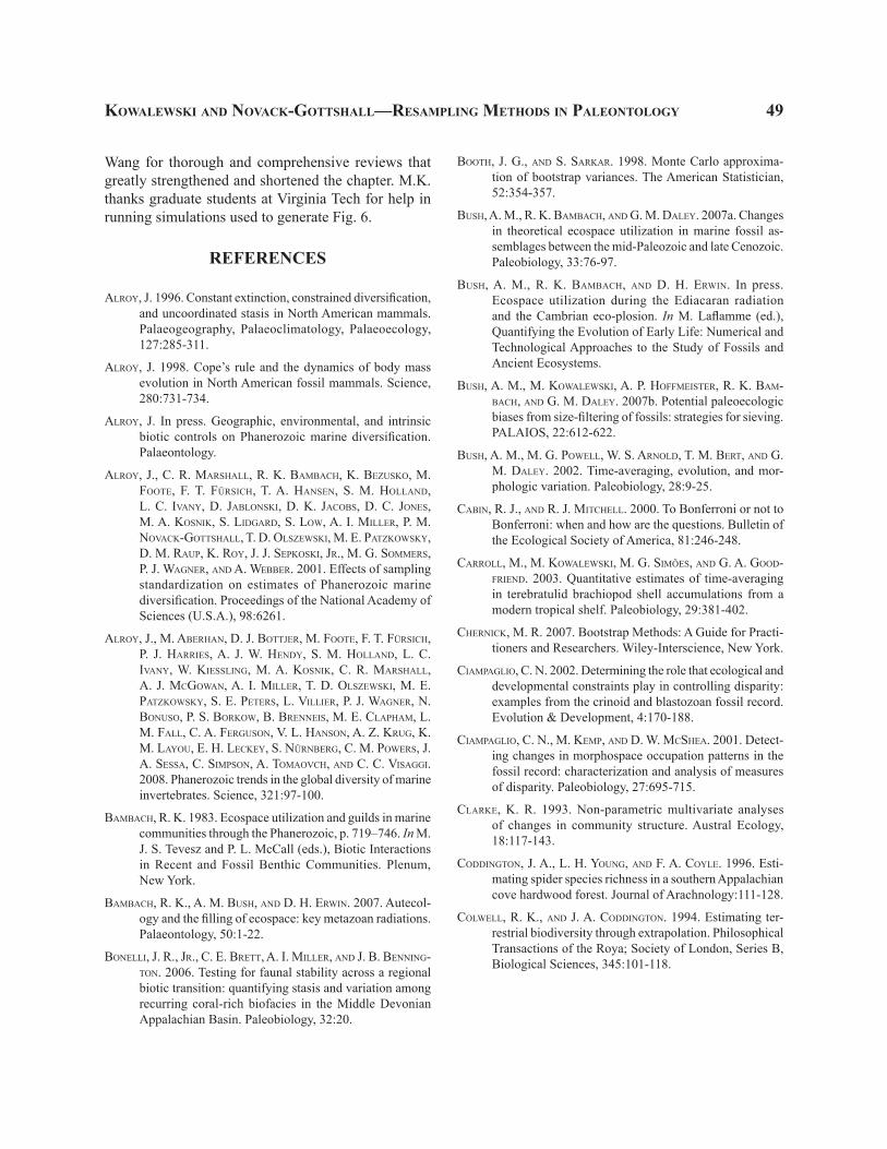
KOWALEWSKI ANd NOVACK-GOTTSHALL—RESAMPLING METHOdS IN PALEONTOLOGy 49
Wang for thorough and comprehensive reviews that greatly strengthened and shortened the chapter. M.K. thanks graduate students at Virginia Tech for help in running simulations used to generate Fig. 6.
reFerences
ALROy, J. 1996. Constant extinction, constrained diversification, and uncoordinated stasis in North American mammals. Palaeogeography, Palaeoclimatology, Palaeoecology, 127:285-311.
ALROy, J. 1998. Cope’s rule and the dynamics of body mass evolution in North American fossil mammals. Science, 280:731-734.
ALROy, J. In press. Geographic, environmental, and intrinsic biotic controls on Phanerozoic marine diversification. Palaeontology.
ALROy, J., C. R. MARSHALL, R. K. BAMBACH, K. BEzuSkO, M. FOOTE, F. T. FüRSICH, T. A. HANSEN, S. M. HOLLAND, L. C. IvANy, D. JABLONSkI, D. K. JACOBS, D. C. JONES, M. A. KOSNIk, S. LIDGARD, S. LOw, A. I. MILLER, P. M. NOvACk-GOTTSHALL, T. D. OLSzEwSkI, M. E. PATzkOwSky, D. M. RAuP, K. ROy, J. J. SEPkOSkI, JR., M. G. SOMMERS, P. J. WAGNER, AND A. WEBBER. 2001. Effects of sampling standardization on estimates of Phanerozoic marine diversification. Proceedings of the National Academy of Sciences (U.S.A.), 98:6261.
ALROy, J., M. ABERHAN, D. J. BOTTjER, M. FOOTE, F. T. FüRSICH, P. J. HARRIES, A. J. W. HENDy, S. M. HOLLAND, L. C. IvANy, W. KIESSLING, M. A. KOSNIk, C. R. MARSHALL, A. J. MCGOwAN, A. I. MILLER, T. D. OLSzEwSkI, M. E. PATzkOwSky, S. E. PETERS, L. VILLIER, P. J. WAGNER, N. BONuSO, P. S. BORkOw, B. BRENNEIS, M. E. CLAPHAM, L. M. FALL, C. A. FERGuSON, V. L. HANSON, A. Z. KRuG, K. M. LAyOu, E. H. LECkEy, S. NüRNBERG, C. M. POwERS, J. A. SESSA, C. SIMPSON, A. TOMAOvCH, AND C. C. VISAGGI. 2008. Phanerozoic trends in the global diversity of marine invertebrates. Science, 321:97-100.
BAMBACH, R. K. 1983. Ecospace utilization and guilds in marine communities through the Phanerozoic, p. 719–746. In M. J. S. Tevesz and P. L. McCall (eds.), Biotic Interactions in Recent and Fossil Benthic Communities. Plenum, New York.
BAMBACH, R. K., A. M. BuSH, AND D. H. ERwIN. 2007. Autecol-ogy and the filling of ecospace: key metazoan radiations. Palaeontology, 50:1-22.
BONELLI, J. R., JR., C. E. BRETT, A. I. MILLER, AND J. B. BENNING-TON. 2006. Testing for faunal stability across a regional biotic transition: quantifying stasis and variation among recurring coral-rich biofacies in the Middle Devonian Appalachian Basin. Paleobiology, 32:20.
BOOTH, J. G., AND S. SARkAR. 1998. Monte Carlo approxima-tion of bootstrap variances. The American Statistician, 52:354-357.
BuSH, A. M., R. K. BAMBACH, AND G. M. DALEy. 2007a. Changes in theoretical ecospace utilization in marine fossil as-semblages between the mid-Paleozoic and late Cenozoic. Paleobiology, 33:76-97.
BuSH, A. M., R. K. BAMBACH, AND D. H. ERwIN. In press. Ecospace utilization during the Ediacaran radiation and the Cambrian eco-plosion. In M. Laflamme (ed.), Quantifying the Evolution of Early Life: Numerical and Technological Approaches to the Study of Fossils and Ancient Ecosystems.
BuSH, A. M., M. KOwALEwSkI, A. P. HOffMEISTER, R. K. BAM-BACH, AND G. M. DALEy. 2007b. Potential paleoecologic biases from size-filtering of fossils: strategies for sieving. PALAIOS, 22:612-622.
BuSH, A. M., M. G. POwELL, W. S. ARNOLD, T. M. BERT, AND G. M. DALEy. 2002. Time-averaging, evolution, and mor-phologic variation. Paleobiology, 28:9-25.
CABIN, R. J., AND R. J. MITCHELL. 2000. To Bonferroni or not to Bonferroni: when and how are the questions. Bulletin of the Ecological Society of America, 81:246-248.
CARROLL, M., M. KOwALEwSkI, M. G. SIMõES, AND G. A. GOOD-fRIEND. 2003. Quantitative estimates of time-averaging in terebratulid brachiopod shell accumulations from a modern tropical shelf. Paleobiology, 29:381-402.
CHERNICk, M. R. 2007. Bootstrap Methods: A Guide for Practi-tioners and Researchers. Wiley-Interscience, New York.
CIAMPAGLIO, C. N. 2002. Determining the role that ecological and developmental constraints play in controlling disparity: examples from the crinoid and blastozoan fossil record. Evolution & Development, 4:170-188.
CIAMPAGLIO, C. N., M. KEMP, AND D. W. MCSHEA. 2001. Detect-ing changes in morphospace occupation patterns in the fossil record: characterization and analysis of measures of disparity. Paleobiology, 27:695-715.
CLARkE, K. R. 1993. Non-parametric multivariate analyses of changes in community structure. Austral Ecology, 18:117-143.
CODDINGTON, J. A., L. H. YOuNG, AND F. A. COyLE. 1996. Esti-mating spider species richness in a southern Appalachian cove hardwood forest. Journal of Arachnology:111-128.
COLwELL, R. K., AND J. A. CODDINGTON. 1994. Estimating ter-restrial biodiversity through extrapolation. Philosophical Transactions of the Roya; Society of London, Series B, Biological Sciences, 345:101-118.
50 the PaleontologIcal socIety PaPers, vol.16
CRAMPTON, J. S., M. FOOTE, A. G. BEu, P. A. MAxwELL, R. A. COOPER, I. MATCHAM, B. A. MARSHALL, AND C. M. JONES. 2006. The ark was full! Constant to declining Cenozoic shallow marine biodiversity on an isolated midlatitude continent. Paleobiology, 32:509-532.
CuRRANO, E. D. 2009. Patchiness and long-term change in early Eocene insect feeding damage. Paleobiology, 35:484-498.
DAvISON, A. C., AND D. V. HINkLEy. 1997. Bootstrap Methods and their Application. Cambridge University Press, Cambridge, UK.
DAvISON, A. C., D. V. HINkLEy, AND E. SCHECHTMAN. 1986. Ef-ficient bootstrap simulation. Biometrika, 73:555-566.
DIACONIS, P., AND B. EfRON. 1983. Computer-intensive methods in statistics. Scientific American, 248:116-130.
DICICCIO, T. J., AND J. P. ROMANO. 1988. A review of bootstrap confidence intervals. Journal of the Royal Statistical Society. Series B (Methodological), 50:338-354.
DIETL, G. P., AND R. R. ALExANDER. 2000. Post-Miocene shift in stereotypic naticid predation on confamilial prey from the mid-Atlantic shelf: coevolution with dangerous prey. PALAIOS, 15:414-429.
EBLE, G. J. 2000. Contrasting evolutionary flexibility in sister groups: disparity and diversity in Mesozoic atelostomate echinoids. Paleobiology, 26:56-79.
EDGINGTON, E., AND P. ONGHENA. 2007. Randomization Tests. Chapman & Hall/CRC, New York.
EfRON, B. 1979. Bootstrap methods: another look at the jack-knife. The Annals of Statistics, 7:1-26.
EfRON, B. 1983. Estimating the error rate of a prediction rule: improvement on cross-validation. Journal of the American Statistical Association, 78:316-331.
EfRON, B. 1987. Better bootstrap confidence intervals. Journal of the American Statistical Association, 82:171-185.
EfRON, B., AND R. J. TIBSHIRANI. 1997. An Introduction to the Bootstrap. Chapman & Hall.
FOOTE, M. 1992. Rarefaction analysis of morphological and taxonomic diversity. Paleobiology, 18:1-16.
FOOTE, M. 1993. Discordance and concordance between morphological and taxonomic diversity. Paleobiology, 19:185-204.
FOOTE, M. 1999. Morphological diversity in the evolutionary radiation of Paleozoic and post-Paleozoic crinoids. Pa-leobiology Memoir, 25 (Supplement):1-116.
FOOTE, M. 2005. Pulsed origination and extinction in the marine realm. Paleobiology, 31:6-20.
FOOTE, M. 2006. Substrate affinity and diversity dynamics of Paleozoic marine animals. Paleobiology, 32:345-366.
GAHN, F. J., AND T. K. BAuMILLER. 2004. A bootstrap analysis for comparative taphonomy applied to Early Mississippian (Kinderhookian) crinoids from the Wassonville Cycle of Iowa. PALAIOS, 19:17-38.
GILINSky, N. L. 1991. Bootstrapping and the fossil record, p. 185-206. In N. L. Gilinsky and P. W. Signor (eds.), Analytical Paleobiology. Short Courses in Paleontology 4. Paleontological Society and University of Tennessee Knoxville, Knoxville, TN.
GILINSky, N. L., AND R. K. BAMBACH. 1986. The evolutionary bootstrap: a new approach to the study of taxonomic diversity. Paleobiology, 12:251-268.
GILINSky, N. L., AND J. B. BENNINGTON. 1994. Estimating num-bers of whole individuals from collections of body parts: a taphonomic limitation of the paleontological record. Paleobiology, 20:245-258.
GLEASON, J. R. 1988. Algorithms for balanced bootstrap simula-tions. The American Statistician, 42:263-266.
GOOD, P. I. 2006. Resampling Methods: A Practical Guide to Data Analysis. Birkhauser, Boston.
GOTELLI, N. J., AND A. M. ELLISON. 2004. A Primer of Ecological Statistics. Sinauer Associates.
GOuLD, S. J., D. M. RAuP, J. J. SEPkOSkI, Jr., T. J. M. SCHOPf, AND D. S. SIMBERLOff. 1977. The shape of evolution: a com-parison of real and random clades. Paleobiology, 3:23-40.
GREy, M., J. W. HAGGART, AND P. L. SMITH. 2008. A new species of Buchia (Bivalvia: Buchiidae) from British Columbia, Canada, with an analysis of buchiid bipolarity. Journal of Paleontology, 82:391-397.
HALL, P. 1992. Efficient bootstrap simulations, p. 127-143. In R. Lepage and L. Billard (eds.), Exploring the Limits of Bootstrap. Wiley, New York City.
HARRINGTON, G. J., AND C. A. JARAMILLO. 2007. Paratropical floral extinction in the late Palaeocene-early Eocene. Journal of the Geological Society, 164:323-332.
HEIM, N. A. 2008. A null biogeographic model for quantifying the role of migration in shaping patterns of global taxonomic richness and differentiation diversity, with implications for Ordovician biogeography. Paleobiology, 34:195-209.
HEIM, N. A. 2009. Stability of regional brachiopod diversity structure across the Mississippian/Pennsylvanian bound-ary. Paleobiology, 35:393.
HERRERA-CuBILLA, A., M. H. DICk, J. A. SANNER, AND J. B. C. JACkSON. 2006. Neogene Cupuladriidae of tropical America. I: Taxonomy of Recent Cupuladria from op-posite sides of the Isthmus of Panama. Journal of Pale-ontology, 80:245-263.
HjORTH, J. S. U. 1994. Computer Intensive Statistical Methods: Validation Model Selection and Bootstrap. Chapman & Hall/CRC, London.
KOWALEWSKI ANd NOVACK-GOTTSHALL—RESAMPLING METHOdS IN PALEONTOLOGy 51
HOffMEISTER, A. P., M. KOwALEwSkI, T. K. BAuMILLER, AND R. K. BAMBACH. 2004. Drilling predation on Permian brachio-pods and bivalves from the Glass Mountains, west Texas. Acta Palaeontologica Polonica, 49:443-454.
HOLDENER, E. J. 1994. Numerical taxonomy of fenestrate bryozoans: evaluation of methodologies and recogni-tion of intraspecific variation. Journal of Paleontology, 68:1201-1214.
HOLLAND, S. M. 1995. The stratigraphic distribution of fossils. Paleobiology, 21:92-109.
HOPkINS, M. J., AND M. WEBSTER. 2009. Ontogeny and geographic variation of a new species of the corynexochine trilobite Zacanthopsis (Dyeran, Cambrian). Journal of Paleontol-ogy, 83:524-547.
HORA, S. C., AND J. B. WILCOx. 1982. Estimation of error rates in several-population discriminant analysis. Journal of Marketing Research, 19:57-61.
HuNT, G., AND R. E. CHAPMAN. 2001. Evaluating hypotheses of instar-grouping in arthropods: a maximum likelihood approach. Paleobiology, 27:466.
HuNTLEy, J. W., S. XIAO, AND M. KOwALEwSkI. 2006. 1.3 billion years of acritarch history: an empirical morphospace ap-proach. Precambrian Research, 144:53-68.
HuNTLEy, J. W., Y. YANES, M. KOwALEwSkI, C. CASTILLO, A. DELGADO-HuERTAS, M. IBáñEz, M. R. ALONSO, J. E. ORTIz, AND T. D. TORRES. 2008. Testing limiting similarity in Qua-ternary terrestrial gastropods. Paleobiology, 34:378-388.
HuRLBERT, S. H. 1971. The nonconcept of species diversity: a critique and alternative parameters. Ecology, 52:577-586.
IvANy, L. C., C. E. BRETT, H. L. B. WALL, P. D. WALL, AND J. C. HANDLEy. 2009. Relative taxonomic and ecologic stability in Devonian marine faunas of New York State: a test of coordinated stasis. Paleobiology, 35:499-524.
KITCHELL, J. A., AND N. MACLEOD. 1988. Macroevolutionary interpretations of symmetry and synchroneity in the fossil record. Science, 240:1190-1195.
KOCH, C. F. 1991. Sampling from the fossil record, p. 4–18. In N. L. Gilinsky and P. W. Signor (eds.), Analytical Paleobiology. Short Courses in Paleontology 4. Paleon-tological Society and University of Tennessee Knoxville, Knoxville, TN.
KOwALEwSkI, M. 1996. Taphonomy of a living fossil; the lingulide brachiopod Glottidia palmeri Dall from Baja California, Mexico. PALAIOS, 11:244-265.
KOwALEwSkI, M., AND S. FINNEGAN. 2010. Theoretical diversity of the marine biosphere. Paleobiology, 36:1-15.
KOwALEwSkI, M., AND J. D. RIMSTIDT. 2003. Average lifetime and age spectra of detrital grains: toward a unifying theory of sedimentary particles. Journal of Geology, 111:427-439.
KOwALEwSkI, M., G. A. GOODfRIEND, AND K. W. FLESSA. 1998. High-resolution estimates of temporal mixing within shell beds: the evils and virtues of time-averaging. Paleobiol-ogy, 24:287-304.
KOwALEwSkI, M., E. DyRESON, J. D. MARCOT, J. A. VARGAS, K. W. FLESSA, AND D. P. HALLMAN. 1997. Phenetic discrimination of biometric simpletons: paleobiological implications of morphospecies in the lingulide brachiopod Glottidia. Paleobiology, 23:444-469.
KOwALEwSkI, M., W. KIESSLING, M. ABERHAN, F. T. FüRSICH, D. SCARPONI, S. L. BARBOuR WOOD, AND A. P. HOff-MEISTER. 2006. Ecological, taxonomic, and taphonomic components of the post-Paleozoic increase in sample-level species diversity of marine benthos. Paleobiology, 32:533-561.
KRAuSE, R. A., JR. 2004. An assessment of morphological fidel-ity in the sub-fossil record of a terebratulide brachiopod. PALAIOS, 19:460-476.
KRAuSE, R. A., JR., S. L. BARBOuR WOOD, M. KOwALEwSkI, D. KAufMAN, C. S. ROMANEk, M. G. SIMOES, AND J. F. WEHM-ILLER. 2010. Quantitative estimates and modeling of time averaging in bivalves and brachiopods. Paleobiology, 36:428-452.
LOMBARDI, C. M., AND S. H. HuRLBERT. 2009. Misprescription and misuse of one-tailed tests. Austral Ecology, 34:447-468.
LuPIA, R. 1999. Discordant morphological disparity and taxonomic diversity during the Cretaceous angiosperm radiation: North American pollen record. Paleobiology, 25:1-28.
MAGuRRAN, A. E. 2003. Measuring Biological Diversity. Wiley-Blackwell, New York City.
MANLy, B. F. J. 2004. Randomization, Bootstrap and Monte Carlo Methods in Biology. Chapman & Hall, Cornwall, Great Britain.
MANLy, B. F. J., AND L. MCALEvEy. 1987. A randomization alternative to the Bonferroni inequality with multiple F tests. Proceedings of the Second International Tampere Conference in Statistics, 2:567-573.
MARkO, P. B., AND J. B. C. JACkSON. 2001. Patterns of morpho-logical diversity among and within arcid bivalve species pairs separated by the Isthmus of Panama. Journal of Paleontology, 75:590-606.
MCLACHLAN, G. J., AND K. E. BASfORD. 1988. Mixture Models: Inference and Applications to Clustering. Marcel Dekker, New York.
MILLER, A. I., AND S. R. CONNOLLy. 2001. Substrate affinities of higher taxa and the Ordovician Radiation. Paleobiology, 27:768-778.
MILLER, A. I., AND M. FOOTE. 1996. Calibrating the Ordovician radiation of marine life: implications for Phanerozoic diversity trends. Paleobiology, 22:304-309.
52 the PaleontologIcal socIety PaPers, vol.16
MONCHOT, H., AND J. LéCHELLE. 2002. Statistical nonparametric methods for the study of fossil populations. Paleobiol-ogy, 28:55.
NAvARRO, N., P. NEIGE, AND D. MARCHAND. 2005. Faunal invasions as a source of morphological constraints and innovations? The diversification of the early Cardioceratidae (Am-monoidea; Middle Jurassic). Paleobiology, 31:98-116.
NOvACk-GOTTSHALL, P. M. 2006. Distinguishing among the four open hypotheses for long-term trends in ecospace diversification: a null model approach. GSA Abstracts with Programs, 38:86.
NOvACk-GOTTSHALL, P. M. 2007. Using a theoretical ecospace to quantify the ecological diversity of Paleozoic and modern marine biotas. Paleobiology, 33:273-294.
NOvACk-GOTTSHALL, P. M. 2008a. Ecosystem-wide body-size trends in Cambrian–Devonian marine invertebrate lin-eages. Paleobiology, 34:210-228.
NOvACk-GOTTSHALL, P. M. 2008b. Modeling community structure across hierarchical scales: A case study using Late Ordovi-cian deep-subtidal assemblages from the Cincinnati Arch. GSA Abstracts with Programs, 40:324.
NOvACk-GOTTSHALL, P. M., AND M. A. LANIER. 2008. Scale-depen-dence of Cope’s rule in body size evolution of Paleozoic brachiopods. Proceedings of the National Academy of Sciences (U.S.A.), 105:5430.
NOvACk-GOTTSHALL, P. M., AND A. I. MILLER. 2003. Comparative taxonomic richness and abundance of Late Ordovician gastropods and bivalves in mollusc-rich strata of the Cincinnati Arch. PALAIOS, 18:559-571.
OLSzEwSkI, T. D., AND M. E. PATzkOwSky. 2001. Measuring recurrence of marine biotic gradients: a case study from the Pennsylvanian-Permian Midcontinent. PALAIOS, 16:444-460.
PANDOLfI, J. M. 1996. Limited membership in Pleistocene reef coral assemblages from the Huon Peninsula, Papua New Guinea: constancy during global change. Paleobiology, 22:152-176.
PERNEGER, T. V. 1998. What’s wrong with Bonferroni adjust-ments. British Medical Journal, 316:1236.
PLOTNICk, R. E. 1989. Application of bootstrap methods to reduced major axis line fitting. Systematic Zoology, 38:144-153.
RAuP, D. M. 1966. Geometric analysis of shell coiling: general problems. Journal of Paleontology, 40:1178-1190.
RAuP, D. M. 1967. Geometric analysis of shell coiling: coiling in ammonoids. Journal of Paleontology, 41:43-65.
RAuP, D. M. 1975. Taxonomic diversity estimation using rarefac-tion. Paleobiology, 1:333-342.
RAuP, D. M. 1977. Stochastic models in evolutionary paleobiol-ogy, p. 59-78. In A. Hallam (ed.), Patterns of Evolution as Illustrated by the Fossil Record.Volume 5. Elsevier Scientific Publishing Company, Amsterdam.
RAuP, D. M. 1979. Size of the Permo-Triassic bottleneck and its evolutionary implications. Science, 206:217-218.
RAuP, D. M., AND S. J. GOuLD. 1974. Stochastic simulation and evolution of morphology—towards a nomothetic pale-ontology. Systematic Zoology, 23:305-322.
RAuP, D. M., AND A. MICHELSON. 1965. Theoretical morphology of the coiled shell. Science, 147:1294-1295.
RAuP, D. M., S. J. GOuLD, T. J. M. SCHOPf, AND D. S. SIMBERLOff. 1973. Stochastic models of phylogeny and the evolution of diversity. Journal of Geology, 81:525-542.
ROSENzwEIG, M. L. 2003. Reconciliation ecology and the future of species diversity. Oryx, 37:194-205.
RuxTON, G. D., AND M. NEuHäuSER. 2010. When should we use one-tailed hypothesis testing? Methods in Ecology and Evolution, 1:114-117.
SANDERS, H. L. 1968. Marine benthic diversity: a comparative study. American Naturalist, 102:243.
SCARPONI, D., AND M. KOwALEwSkI. 2007. Sequence stratigraphic anatomy of diversity patterns: Late Quaternary benthic mollusks of the Po Plain, Italy. PALAIOS, 22:296-305.
SHEN, B., L. DONG, S. XIAO, AND M. KOwALEwSkI. 2008. The Avalon explosion: evolution of Ediacara morphospace. Science, 319:81-84.
SIEGfRIED, T. 2010. Odds are, it’s wrong: Science fails to face the shortcomings of statistics. Science News, 177:26.
SIMS, H. J., AND K. J. MCCONwAy. 2003. Nonstochastic variation of species-level diversification rates within angiosperms. Evolution, 57:460-479.
SOkAL, R. R., AND F. J. ROHLf. 1995. Biometry. W.H. Freeman and Company, New York, 887 p.
STANLEy, S. M., P. W. SIGNOR, S. LIDGARD, AND A. F. KARR. 1981. Natural clades differ from “random” clades: simulations and analyses. Paleobiology, 7:115-127.
TIPPER, J. C. 1979. Rarefaction and rarefiction: the use and abuse of a method in paleoecology. Paleobiology, 5:423-434.
TOMASOvyCH, A., AND S. M. KIDwELL. 2009. Preservation of spa-tial and environmental gradients by death assemblages. Paleobiology, 35:119-145.
TukEy, J. W. 1958. Bias and confidence in not quite large samples. Annals of Mathematical Statistics, 29:614.
WANG, S. C. 2003. On the continuity of background and mass extinction. Paleobiology, 29:455.
WINCH, R. F., AND D. T. CAMPBELL. 1969. Proof? No. Evidence? Yes. The significance of tests of significance. American Sociologist, 4:140-143.
KOWALEWSKI ANd NOVACK-GOTTSHALL—RESAMPLING METHOdS IN PALEONTOLOGy 53
aPPendIX 1. glossary oF terMs.
The glossary below represents our best attempt to identify clear and generally accepted definitions of common terms used in the resampling literature. Such definitions are not always clearly explained in different resampling and statistical texts, and in some cases, different authors use the same term in different ways. Occasionally, some terms have been used (either implicitly or occasionally explicitly) in a contradictory manner. Even worse, different authors—the current chapter authors included—have used different terms for the same concept. In such cases, we used majority rule to assign definitions, but noted common synonyms (e.g., exhaustive randomization and exact permutation tests). See the chapter text for specific examples where definitions are commonly conflated. We hope that this glossary will prove a useful reference for clarifying the resampling terminology and making the literature more accessible. Major sources for definitions include Sokal and Rohlf (1995), Good (2006), and Manly (2004).
Alpha: See type I error (alpha, significance level).Balanced resampling design: Resampling design
in which all observations are used the same number of times across the resampling method, ensuring efficient and precise estimation of some distribution moments such as the mean.
Bonferroni correction: Adjustment to individual alpha levels when conducting multiple independent tests or making multiple independent comparisons to ensure that the overall alpha level remains as specified.
Bootstrapping: Resampling method in which samples are taken at random and with replacement from an existing sample.
Central limit theorem: Theorem stating that as sample size increases, the means of samples drawn from a population of any distribution (assuming independent variables with finite means and variances) will approach the normal distribution.
Combination: An arrangement of objects in which their order does not matter. For example, set 1-2-3 is the same combination as set 3-2-1.
Combination with repetition (replacement): A combination in which objects are sampled with replace-ment; this is essentially a bootstrap. For example, sets 1-2-2 and 2-2-1 are two identical combinations with replacement from sample 1-2-3.
Data-based Monte Carlo: Resampling analysis that uses random sampling of empirical data within the framework of a specified model to evaluate hypotheses.
Exhaustive bootstrap: Bootstrap analysis using an exhaustive resampling design (i.e., a complete enumeration).
Exhaustive randomization (exact permutation test): See systematic data permutation.
Exhaustive resampling design: Resampling de-sign in which all possible combinations are resampled once and only once.
Exhaustive resampling distribution: See system-atic reference set.
Generalized (serial) Monte Carlo test: Resam-pling analysis, generally used in situations involving Markovian autocorrelation, where an iterative series of random swaps of individual empirical data values is used to generate a resampling distribution.
Implicit Monte Carlo: See model-based Monte Carlo.
Iteration (replicate): Number of times that resampling is repeated. (Following general usage, we advise using iteration as a noun and replicate as a verb or adjective, as in, “The bootstrap algorithm used 10,000 iterations in which replicate pairs of samples were resampled with replacement.”)
Jackknife: Resampling method in which a sub-sample is made by removing a single observation at random from an existing sample. (But see text for additional variants on the jackknife.)
Model-based Monte Carlo (implicit Monte Carlo): Resampling analysis that uses random sampling of some parametric distribution within the framework of a specified model to evaluate hypotheses.
Monte Carlo approximation: Any resampling design that uses random sampling to approximate an systematic reference set (exhaustive resampling distribution).
Parametric bootstrap: Bootstrap resampling in which sampling is made from a parametric distribution instead of the empirical sample itself.
Percentile confidence interval (naïve or primitive confidence intervals): Confidence interval obtained by
WOOD, A. R., M. L. ZELDITCH, A. N. ROuNTREy, T. P. EITING, H. D. SHEETS, AND P. D. GINGERICH. 2007. Multivariate stasis in the dental morphology of the Paleocene-Eocene condylarth Ectocion. Paleobiology, 33:248-260.
ZAR, J. H. 2009. Biostatistical Analysis. Prentice Hall, Engle-wood Cliffs, NJ, 718 p.
54 the PaleontologIcal socIety PaPers, vol.16
choosing fixed percentiles in the tails of the resampling distribution.
Permutation: An arrangement of objects in which their order matters. For example, set 1-2-3 is a different permutation than set 3-2-1.
Power: Probability of rejecting the hypothesis when the null hypothesis is false. Calculated as 1 minus the probability of making a Type II error.
Probability density function: A continuous distri-bution, ordinarily illustrated as a curve, that represents the probability of observing a variable in a particular range. (Compare with probability mass functions that are discrete distributions.)
Probability mass function: A discrete distribution, ordinarily illustrated as a histogram that represents the probability of observing a variable of a particular value. (Compare with probability density functions that are continuous distributions.)
p-value: The probability of observing a statistic as extreme or more extreme that that actually observed, if the null hypothesis were true.
Randomization (permutation): Nonparametric resampling method applied solely to a particular data set (i.e., not generalizable to the sampled population) that involves re-assigning observations without replace-ment to test the probability of observing some outcome.
Randomized data permutation: Permutation (randomization) test that randomly samples many data combinations to approximate an exhaustive resampling distribution (systematic reference set).
Rarefaction: Form of sample-standardization in which a parameter of interest is estimated for sample sizes smaller than that of the analyzed datasets by sub-sampling from those datasets without replacement. The resampling estimates can be done for one preset sample size (this protocol is often referred as subsampling) or for a successive series of increasingly smaller sample sizes, so the parameter value can be plotted as a func-tion of sample size (rarefaction curve).
Reference set (resampling distribution): See resampling distribution.
Replicate (iterate): Generally used as the adjec-tival or verb form of iteration. See Iteration (replicate) for details.
Resampling distribution (reference set): Distribu-tion of statistics obtained by a particular resampling method.
Sample-standardization: Methods in which all
datasets are standardized simultaneously in some fashion to make them more comparable to each other. Rarefaction/subsampling is a simple example of a standardization protocol, but such protocols may be much more complex.
Sampling distribution: A distribution of some statistic of interest sampled randomly at a given sample size from a population of observations.
Significance level: See type I error (alpha, sig-nificance level).
Subsampling: See rarefactionSystematic data permutation: Permutation test
involving all possible combinations of data to calcu-late an exact probabilistic outcome from a systematic reference set.
Systematic reference set: An exhaustive resam-pling distribution.
Two-sample bootstrap test: Bootstrap equivalent to a two-sample test (e.g., parametric t-test, non-para-metric Mann-Whitney [Wilcoxon rank-sum] test, etc.).
Type I error (alpha, significance level): Error in which a true primary (null) hypothesis is rejected. This is customarily symbolized as alpha=0.X, corresponding to a significance level of X%.
Type II error: Error in which a false null hypoth-esis is not rejected.
Uniform resampling design: Resampling design in which observations always are drawn at random with probability of 1/n, where n is the number of observa-tions being resampled. (Unlike balanced resampling, this design draws some observations more than oth-ers, producing an inefficient estimation of distribution moments.)
reFerences
GOOD, P. I. 2006. Resampling Methods: A Practical Guide to Data Analysis. Birkhauser, Boston.
MANLy, B. F. J. 2004. Randomization, Bootstrap and Monte Carlo Methods in Biology. Chapman & Hall, Cornwall, Great Britain.
SOkAL, R. R., AND F. J. ROHLf. 1995. Biometry. W.H. Freeman and Company, New York.