Embed Size (px)
Citation preview

Research ArticleExperimental Studies on Finite Element ModelUpdating for a Heated Beam-Like Structure
Kaipeng Sun12 Yonghui Zhao1 and Haiyan Hu13
1State Key Laboratory of Mechanics and Control of Mechanical Structures Nanjing University of Aeronautics and AstronauticsNanjing 210016 China2Shanghai Institute of Satellite Engineering Shanghai 200240 China3MOE Key Laboratory of Dynamics and Control of Flight Vehicle School of Aerospace Engineering Beijing Institute of TechnologyBeijing 100081 China
Correspondence should be addressed to Haiyan Hu hhyaenuaaeducn
Received 22 September 2014 Revised 6 December 2014 Accepted 11 December 2014
Academic Editor Tony Murmu
Copyright copy 2015 Kaipeng Sun et al This is an open access article distributed under the Creative Commons Attribution Licensewhich permits unrestricted use distribution and reproduction in any medium provided the original work is properly cited
An experimental study was made for the identification procedure of time-varying modal parameters and the finite element modelupdating technique of a beam-like thermal structure in both steady and unsteady high temperature environments An improvedtime-varying autoregressive method was proposed first to extract the instantaneous natural frequencies of the structure in theunsteady high temperature environment Based on the identified modal parameters then a finite element model for the structurewas updated by using Kriging meta-model and optimization-based finite-element model updating method The temperature-dependent parameters to be updated were expressed as low-order polynomials of temperature increase and the finite elementmodel updating problem was solved by updating several coefficients of the polynomials The experimental results demonstratedthe effectiveness of the time-varyingmodal parameter identificationmethod and showed that the instantaneous natural frequenciesof the updated model well tracked the trends of the measured values with high accuracy
1 Introduction
Hypersonic vehicles are subject to very tough aerodynamicload and heating during their missions in the Earthrsquos atmo-sphere The aerodynamic heating is extremely importantbecause high temperature can affect the structural behaviorin several detrimental ways [1] The elevated temperature notonly degrades the ability of structure materials to withstandloads but also produces the thermal stresses in heatedstructures In addition the thermal stresses increase defor-mation change buckling loads and alter flutter behavior Forexample the studies [2ndash5] reported that even a minor changeof temperature would result in a significant alteration innatural frequencies of a beam because of the thermal stresseswhen the beam was constrained Thermal modal testingtechniques can provide quantitative analysis for the effect ofthe thermal load [6] Since the 1950s many experiments havebeen done in NASA Langley and Dryden research centers
for the metal and the composite panels [7 8] the X-15 wing[9] and the X-34 FASTRAC Composite Rocket Nozzle [10]The aforementioned studies have primarily focused on thedynamical properties of thermal structures in steady hightemperature environments (SHTEs)
As a matter of fact thermal structures in unsteady hightemperature environments (UHTEs) for example hyper-sonic vehicles subjected to unsteady aerodynamic heatinghave the characteristic of time-varying multiphysics fieldsThe identification of time-varying modal parameters is theforefront of inverse problems in structural dynamics Therehave been numerous theoretical and experimental studieson the identification of time-varying modal parameters forengineering structures The special issue [11] of MechanicalSystems and Signal Processing on the identification of timevarying structures and systems in 2014 offered a survey ofthe field in its current state reflected recent developmentsand also pointed out into the future in various aspects of
Hindawi Publishing CorporationShock and VibrationVolume 2015 Article ID 143254 15 pageshttpdxdoiorg1011552015143254
2 Shock and Vibration
the theories and applications Although recent years havewitnessed successful identifications of time-varying modalparameters of many engineering systems such as vehicle-bridge systems [12 13] machine condition monitoring sys-tems [14] flexible manipulators [15] and civil structures [1617] their applications to thermal structures in temperature-varying environment are still not available Yu et al [18]proposed an undetermined blind source separation methodto investigate the thermal effect on the modal parametersof a TC4 titanium-alloy column in a temperature-varyingenvironmentThey [19] also developed a time-varying modalparameter identification algorithm based on finite-data-window PAST and used it to investigate the effect of varyingtemperature and heating speed on the natural frequencies of atrapezoidal TA15 titanium-alloy plate To the best knowledgeof authors considerably less attention has been paid tothe finite element model updating (FEMU) for thermalstructures especially based on the identified time-varyingmodal parameters in UHTEs
Finite element (FE) modelling has received widespreadacceptance andwitnessed applications in various engineeringdisciplines Hence the FE model updating (FEMU) hasbecome a useful tool to improve the modelling assumptionsand parameters until a correlation between the analyti-cal predictions and experimental results satisfies practicalrequirements Mottershead and Friswell [20] comprehen-sively reviewed the model updating methods of structuralmodels In Marwalarsquos work [21] numerous computationalintelligence techniques were introduced and applied to FEmodel updating with in-depth comparisons As a mostwidely used method in FEMU the iterative method hasbeen formulated as an optimization problem and often basedon sensitivity analysis [22] and computational intelligencetechniques [23ndash25] Generally the optimization procedure isnonlinear and complex for a complicated FEMU problemIn recent years the particle swarm optimization (PSO)technique has been developed to implement the optimizationprocedure
The structural FE models with many geometric andphysical parameters to be updated may involve a largenumber of computations and need to be constructed byone of commercial finite element analysis packages suchas COMSOL ANSYS and NASTRAN Hence higher timeconsumption may be the disadvantage for the optimization-based algorithms due to their iterative strategy and repeatedanalysis in simulation models during the optimization pro-cess One way to overcome the difficulty of time consumptionand FE package-related problems during the optimization-based model updating is to replace the FE model by anapproximate surrogatereplacement meta-model that is fast-running and has fewer parameters involved Simpson [26]made a comparison of response surface and Kriging modelswhich are the two commonly used meta-models and drew aconclusion that both approximations predict reasonably wellwith the Kriging models having a slight overall advantagebecause of the lower root mean squared error values
The meta-model method for damage detection and relia-bility analysis has a long history However the Kriging meta-model (KMM) method for structural FEMU is somewhat
new especially for thermal structures in temperature-varyingenvironment As a continuation of authorsrsquo work [27 28]this paper presents KMM-PSO based FE model updatingand selection based on the experimentally identified time-invariant and time-varying modal parameters of a thermalstructure
The remainder is organized as follows In Section 2 theFE model updating and selection for a thermal structureis formulated and two objective functions are given forthe PSO An overview of PSO and a brief introductionto the time-varying autoregressive method for output onlyidentification are also presented The Kriging meta-modelis introduced to employ the PSO based FE model updatingand selection In Section 3 four groups of experiments arediscussed for the modal parameters of a beam-like structurein room temperature environment SHTE and UHTE InSection 4 the Kriging meta-model based FE model updatingand selection procedure is carried out to update the software-based FE model Finally some conclusions are drawn inSection 5
2 Formulation of FEMU forThermal Structures
21 Problem Description A linear thermal structure subjectto unsteady heating can be described in terms of the dis-tributed mass damping and stiffness matrices of the struc-ture in time domain via the following differential equation
Mx (119905) + C (119905) x (119905) + K (119905) x (119905) = f (119905) (1)
The real eigen-value problem for the 119895th mode reads
(K (119905) minus 120596
2
119895M)120593119895= 0 (2)
where the detailed meanings of the physical quantities in theabove two equations can be found in [28]
The traditional FE model updating process is achievedby identifying the correct mass and stiffness matrices whichare generally time-invariant This study however has to dealwith a time-variant FE model updating process because thesystem matrices change over time when the temperature-dependent material and temperature-dependent boundaryconditions are taken into consideration Afterwards usingthemeasured data the correctmass and stiffnessmatrices canbe obtained by identifying the correct material parameters ofthe structure and the appropriate boundary conditions underdifferent temperature conditions
For simplicity the thermal structure of concern is a kindof slender or thin-walled structures such as beams and platessubject to uniform heating with a uniformly distributedtemperature field119879(119909 119910 119911 119905) equiv 119879(119905) In other words the heattransfer process is neglected in the study Let 120579(119905) denote thetemperature increase in the thermal structure as follows
120579 (119905) = 119879 (119905) minus 119879ref (3)
where 119879ref is the reference temperature For the FEMU prob-lem of the thermal structure subject to unsteady heating the
Shock and Vibration 3
system parameters to be identified depend on the transienttemperature and can be expressed as
Γ119901= flowastℓ(120579) = P
0+ P1120579 + P2120579
2+ P3120579
3+ sdot sdot sdot (4)
where Γ119901is the parameter vector including the temperature-
dependent material and boundary parameters to be cor-rected and flowast
ℓis the general function of the temperature
increase 120579 In general flowastℓcan be expressed as a low-order poly-
nomial for example a linear quadratic or cubic functionin which ℓ represents the highest order of the polynomialThen the target parameters to be corrected change fromtemperature-dependent Γ
119901to a constant parameter vectorP
119896
119896 = 0 1 2 3
22 Objective Function for FEMU at Reference TemperatureIn a reference temperature environment (RTE) to correctlyidentify the moduli of elasticity that gives the updated FEmodel the following objective function which measures thedistance between the measured modal data and the modaldata predicted by FE model should be minimized
119869
0=
119873
sum
119895=1
120574
119895
1003817
1003817
1003817
1003817
1003817
1003817
1003817
1003817
1003817
1003817
119891
meta119895
minus 119891
exp119895
119891
exp119895
1003817
1003817
1003817
1003817
1003817
1003817
1003817
1003817
1003817
1003817
2
(5)
where 1198690is the error function or objective function sdot is the
Euclidean norm 120574119895is the weighted factor for the 119895th mode
and 119873 is the number of measured modes respectively In(5) 119891meta119895
is the 119895th instantaneous natural frequency obtainedfrom the meta-model and 119891
exp119895
is the 119895th instantaneousnatural frequency identified from the measured responses ina thermal-structural experiment based on the identificationmethod for the time-invariant modal parameters
Thus the process of FEMUmay be viewed as an optimiza-tion problem as follows
find P0
min 119869
0
st P1198970le P0le P1199060
(6)
where 119897 and 119906 represent the lower and upper bounds of theparameter coefficient vector P
0 respectively
23 Objective Function for FEMU in a UHTE After anupdated model in the RTE is achieved the FEMU canbe performed in a UHTE which contextually means thatthe parameters to be corrected in this subsection becomethe constant parameter vector P
119896(119896 = 0 1 2 3) in (4)
It should be noted that P0here represents several special
parameters that cannot be identified in an RTEThe constantcoefficient of thermal expansion for example has no effecton the stiffness matrix of the FE model and thus cannot beidentified in an RTE but must be updated in a UHTE
Furthermore a new problem arises when the tempera-ture-dependent parameter is approximated as a low-orderpolynomial Because it is impossible to knowapriori the exact
order of polynomial flowastℓin (4) a parameter vector expressed
by polynomials of different orders should be considered Ingeneral it is known that the higher the order is the smallerthe deviations between test and analysis are However thepurpose of FEMU is to predict the structural response topredict the effects of structural modifications or to serve asa substructure model to be assembled as part of a model ofthe overall structure From this viewpoint for simplicity onemay use a low order expansion for the material properties Ifthe order is fixed to the maximal value one would manuallyaccept or reject the high-order terms by identifying whetherthe coefficient is close enough to zero If any terms areneglected the deviations between test and analysis shouldbe reexamined Therefore the potential problems in theFEMU procedure are not only how to determine thoseparameters but also how to select the updated model Toavoid establishing many models for FEMU and manuallyselecting the updated model it is preferable to have anall-in-one procedure for both updating and selection ThePSO framework allows this simultaneous updating of allcompetingmodels and selection of the bestmodelHence thetwo aforementioned problems can be solved by minimisingan integrated objective (or fitness) function
A number of fitness or objective functions have beenavailable so far Most previous studies have sought a modelwith the fewest updating parameters needed to produce FEmodel results that are closest to measured results In thisstudy the Akaike information criterion (AIC) was used torepresent the integrated objective functionwith an additionalterm to treat ill-conditioned and noisy systems AIC can bedescribed by the following equation
119869
1=
1
119873sp
119873
sum
119895=1
119873sp
sum
119896=1
120574
119895
1003817
1003817
1003817
1003817
1003817
1003817
1003817
1003817
1003817
1003817
119891
meta119895
(119905
119896) minus 119891
exp119895
(119905
119896)
119891
exp119895
(119905
119896)
1003817
1003817
1003817
1003817
1003817
1003817
1003817
1003817
1003817
1003817
2
(7)
119869
2= 119873 log (119869
1+ 120582
2 10038171003817
1003817
1003817
L (P minus Plowast)1003817100381710038171003817
2
) + 120581119889 (8)
with
119889 = ℓ
1+ ℓ
2+ sdot sdot sdot + ℓ
119873119901 (9)
where119873sp is the number of samplings 119891meta119895
(119905
119896) and 119891exp
119895(119905
119896)
are frequencies at time 119905119896 and Plowast is the initial estimate of
parameter P respectively The second term in the bracketrepresents regularization where the parameter weightingmatrix L should be chosen to reflect the uncertainty in theparameter estimation and L = I represents the classicalTikhonov regularization Link [29] suggested that the factor120582
2 lies in the range of [0 03] High 120582 values are used if thereare many insensitive parameters and if the inverse problemis strongly ill-conditioned The second term of the aboveequation is known as the model complexity penalty termin which 120581 is a weighting factor and ℓ
119896(119896 = 1 2 119873
119901)
represents the highest order of the 119896th polynomial119873119901is the
dimension of the parameter vector
4 Shock and Vibration
Start
Input training dataparameters P
Software-based modalanalyses
Output training resultsnature frequencies
Build Kriging meta-model
Output Kriging predictor
Yes
Initialize particle swarm
Stoppingcriteria
Yes
End
MSEacceptable
No
Kriging meta-model
PSO based FEMU
Nature frequencies fmeta
Set PSO parameters Pk(k = 0 1 2)
Calculate objective function in FEMUapproach for each particle swarm
Find the minimum of for all competing models
Evaluate value of
Output optimizedPk and its order
No
Update parameters(pbestk gbest velocity and position)
J2
J2
J2
Figure 1 Flow chart of Kriging meta-model (left dashed block) and particle swarm optimization based finite element model updating (rightdashed block)
Similarly to the FEMU in an RTE the optimizationprocess here may be expressed as follows
find P119896 119896 = 0 1 2 3
min 119869
2
st P119897119896le P119896le P119906119896
(10)
Figure 1 illustrates the detailed flow chart of the Krigingmeta-model and the particle swarm optimization based FEmodel updating and selection In the left dashed block aKriging meta-model is introduced to overcome the difficultyof time consumption because of the quantities of iterationsduring the updating process In the right dashed blockmodalparameters analyzed from Kriging meta-model and experi-mentally identified by time-varying autoregressive (TVAR)method are used to establish the objective function for thePSO based FE model updating and selection Therefore thenext 3 subsections briefly introduce the stochastic optimiza-tion technique the Kriging meta-modeling and the time-varying autoregressive method and their relevance to the FEmodel updating and selection for thermal structures
24 Stochastic Optimization Technique In this study PSOtechnique is employed to deal with the optimization prob-lems described in (6) and (10) PSO is a population-basedstochastic optimization technique developed by Eberhart andKennedy [30] in 1995 and inspired by the social behavior ofbird flocks and fish schools The PSO procedure begins witha group of random particles and then searches for optima byupdating generationsThe PSO shares many similarities withevolutionary computation techniques such as genetic algo-rithms (GAs) [24] However it has no evolution operatorssuch as crossover or mutation In the PSO particles updatethemselves with an internal velocity and also have memoryand one-way information sharing mechanism
Similarly to GA the algorithm begins with generating agroup of random particles called a swarm At each iterationthe particles evaluate their fitness (positions relative to thegoal) and share memories of their best positions with theswarm Subsequently each particle updates its velocity andposition according to its best previous position (denoted bypbest) and that of the global best particle (denoted by gbest)which has far been found in the swarm Let the position of aparticle be denoted by 119909
119896isin R119899 and let V
119896be its velocityThey
both are initially and randomly chosen and then iteratively
Shock and Vibration 5
updated according to two formulae The following formulais used to update the particlersquos velocity and position asdetermined by Shi and Eberhart [31]
V119896= 119908 sdot V
119896+ 119888
1sdot 119903
1sdot (119901119887119890119904119905
119896minus 119909
119896)
+ 119888
2sdot 119903
2sdot (119892119887119890119904119905 minus 119909
119896)
119909
119896lArr997904 119909
119896+ V119896
(11)
where 119908 is an inertia coefficient that balances the global andlocal search 119903
1and 1199032are random numbers in the range [0 1]
updated at each generation to prevent convergence on localoptima and 119888
1and 119888
2are the learning factors that control
the influence of 119901119887119890119904119905119896and 119892119887119890119904119905 during the search process
Typically 1198881and 1198882are set to be 2 for the sake of convergence
[31]To avoid any physically unrealizable system matrix and
the thermal buckling which easily occurs at extremely hightemperatures artificial position boundaries should be set foreach particle There are four types of boundaries namelyabsorbing reflecting invisible and damping boundaries assummarized in [32] The damping boundary can providea much robust and consistent optimization performance ascompared with other boundary conditions and thus wasused in this study In addition to enforcing search-spaceboundaries after updating a particlersquos position it is alsocustomary to impose limitations on the distance where aparticle can move in a single step [33] which is done bylimiting the velocity to a maximum value with the purposeof controlling the global exploration ability of the particleswarm and preventing the velocity from moving towardsinfinity
In the implementation of FE model updating and selec-tion the parameters P
119896(119896 = 0 1 2 3) are usually set to be
positions of particles for stochastic optimization techniqueThe above updating process should be repeated until aspecified convergence value or total generation number isreachedThis way an optimal process for FE model updatingand selection can be achieved
25 Kriging Meta-Modeling For completeness a briefdescription of the Kriging meta-modeling is given in thissubsection Kriging was named after the pioneering workof D G Krige a South African Mining Engineer and wasformally developed by Matheron [34] Universal Krigingestimates the response 119884(x
lowast) at an untried site x
lowastas the
sum of a polynomial trend model f(xlowast)120573 and a systematic
departure term 119911(xlowast) representing low (large scale) and high
frequency (small scale) variations around the trend model[35]
119884 (xlowast) = f (x
lowast)120573 + 119911 (x
lowast) (12)
where f(xlowast) = [1198911
(xlowast) 119891
2(xlowast) sdot sdot sdot 119891
119872(xlowast)] and120573 = [120573
1120573
2
sdot sdot sdot 120573
119872]
T are the regression model and the regressioncoefficients respectively In the right hand of (12) the firstterm is the mean value which can be thought as a globallyvalid trend function And the second term 119911(x
lowast) is a Gaussian
distributed error term with zero mean and variance 1205902 Thecovariance matrix of 119911(x) is given by
V (119911 (x)) = 120590
2R119899119904times119899119904
(13)
In (13) each element119877119894119895ofR119899119904times119899119904
defined as119877(x119894 x119895) is the
spatial correlation function between any two of the 119899119904sample
points x119894and x119895
In the current simulation the term 119903 represents thedimension of vector x and the linear regression model ischosen for the mean part of the Kriging function [36]Accordingly 119891
119895(x) can be expressed as
119891
1(x) = 1 119891
2(x) = 119909
1
119891
3(x) = 119909
2 119891
1+119903(x) = 119909
119903
(14)
The Gaussian correlation function 119877 is taken as
119877 (x119894 x119895) =
119903
prod
119896=1
exp (minus119901119896
1003816
1003816
1003816
1003816
1003816
x(119896)119894
minus x(119896)119895
1003816
1003816
1003816
1003816
1003816
2
) (15)
where x(119896)119894
is the 119896th component of the 119894th sample point and119901
119896is the unknown correlation parameter which needs to be
fitted by optimizationTo construct the Kriging model the values of the
regression coefficients 120573 = [1205731120573
2sdot sdot sdot 120573
119872]
T must beapproximated by using the generalized least squares theoryat first Then the fitting correlation parameters 119901
119896can be
quantified by using the maximum likelihood estimationThegeneralized least-squares estimates of 120573 and 1205902 representedby 120573 and 2 respectively are given in detail as
120573 = (FTRminus1F)minus1
FTRminus1y
2=
(y minus F120573)TRminus1 (y minus F120573)119899
119904
(16)
where y and F are the 119899119904times 1 vector of output and the 119899
119904times 119899
119904
matrix at the sample inputs respectively which are expressedas
y =[
[
[
[
[
119910
1
119910
2
119910
119899119904
]
]
]
]
]
F =
[
[
[
[
[
119891
1(x1) 119891
2(x1) sdot sdot sdot 119891
119903+1(x1)
119891
1(x2) 119891
2(x2) sdot sdot sdot 119891
119903+1(x2)
d
119891
1(x119899119904) 119891
2(x119899119904) sdot sdot sdot 119891
119903+1(x119899119904)
]
]
]
]
]
(17)
With the vector r = [119877(xlowast x1) 119877(x
lowast x2) sdot sdot sdot 119877(x
lowast
x119899119904)]
T the prediction at the unsampled location xlowastcan be
obtained as
119884 (xlowast) = f (x
lowast)
120573 + rTRminus1 (y minus F120573) (18)
6 Shock and Vibration
For the FEMU problem of thermal structures parame-ters Γ
119901defined in (4) including the temperature-dependent
material and boundary parameters to be corrected are takenas input parameters of Kriging meta-model and the outputparameters are usually modal parameters such as naturalfrequencies or modal shapes
Before the Kriging predictor is used in structural FEmodel updating it should be verified to check whetherthe meta-model has enough accuracy Sacks et al statedthat the cross-validation and integrate mean square errorcan be utilized to assess the accuracy of a Kriging modelThe pointwise (local) estimate of actual error in Krigingapproximation was given by computing the mean squarederror (MSE) 120593(x) as follows [36]
120593 (x) =
2(1 + u (x)T (FTRminus1F) u (x) minus r (x)T Rminus1r (x))
u (x) = FTRminus1r (x) minus f (x) (19)
where 2 is the process variance defined in (16) and 1 is thevector of ones
26 Brief Description of the TVAR Method Identifying thetime-varying modal parameters is an important issue inthe FE model updating and selection for thermoelasticstructures Time-varying autoregressive method is one of themost popular time-frequency analysis methods for outputonly identification
This subsection deals with a TVAR process 119909(119905) (egdisplacement velocity or acceleration) of order 119901 in adiscrete-time as the following
119909 (119905) = minus
119901
sum
119894=1
119886
119897(119905) 119909 (119905 minus 119897) + 119890 (119905) (20)
where 119890(119905) is a stationary white noise process with zero meanand variance 1205902 and 119886
119897(119905) 119897 = 1 2 119901 are the TVAR
coefficientsUsing the basis function expansion and regression
approach the TVARprocess 119909(119905) of order119901 in a discrete-timecan be expressed in matrix form as
119909 (119905) = minusXT119905A + 119890 (119905)
(21)
where
AT= [119886
10 119886
1119898 119886
1199010 119886
119901119898]
XT119905= [119909 (119905 minus 1) 119892
0(119905) 119909 (119905 minus 1) 119892
119898(119905)
119909 (119905 minus 119901) 119892
0(119905) 119909 (119905 minus 119901) 119892
119898(119905)]
(22)
119890(119905) is a stationary white noise process with zero mean andvariance 1205902 119886
119897119896and 119898 are the weighted coefficients and the
dimension of the basis functions 119892119896(119905) 119896 = 0 1 119898
respectivelyThe recursive least square (RLS) estimation and exponen-
tial forgetting method with a constant forgetting factor are
used here such that the parameter estimation algorithm canbe written as
A119873+1
=
A119873minus P119873X119873(120582 + XT
119873P119873X119873)
minus1
sdot (119909 (119873 + 1) + XT119873A119873)
P119873+1
=
1
120582
[P119873minus P119873X119873(120582 + XT
119873P119873X119873)
minus1
XT119873P119873]
(23)
where the forgetting factor 120582 is chosen in the interval (0 1]and is typically close to one The initial value of A and P canbe selected as A
0= 0 P
0= 120583I where 120583 ≫ 1 and I is an
identity matrixOnce the TVAR coefficients are obtained the instanta-
neous natural frequencies can be derived from the conjugateroots 119904
119895(119905) 119904lowast119895(119905) of the time-varying transfer function corre-
sponding to the TVAR model as the following
119891
119895(119905) =
1
2120587Δ119905
radicln 119904119895(119905) sdot ln 119904lowast
119895(119905) (24)
where Δ119905 is the time-discretization step
3 Experimental Studies on a Cantilever Beam
In this study experimental modal analysis and operationalmodal analysis were carried out to obtain the time-invariantand time-varyingmodal parameters respectively in differenttemperature environments The experimental object here isa cantilever beam made of aluminum installed in a movablebox-type resistance furnace as shown as (a) and (b) inFigure 2 The beam was dynamically driven by a hammerimpact or a vibration shaker excitation in experiments Adouble-lug-type connector was used to connect the beamand the vibration shaker when the beam was heated by thefurnace where only the vibration shaker provided feasibleexcitations It should be emphasized that the mass of theconnector should not be neglected in modal analysis Forsimplicity hence the terms ldquobeam Ardquo and ldquobeam Brdquo areused hereinafter for the cantilever beam without the double-lug-type connector and with the double-lug-type connectorrespectively
Figure 2(c) shows the schematic framework of experi-mental setup where beam B is excited by a vibration shakerTable 1 lists four groups of experiments for different cases Forall groups the velocity responses of the beam were measuredby using a laser vibrometer as a noncontacted measurementtechnique
31 The First and Second Groups of Experiments In the firstand second groups of experiments the frequency responsesof beam A and beam B were measured via a hammer impactat room temperature respectively Without loss of generalitythe room temperature was assumed to be reference temper-ature Figure 3 illustrates the amplitude-frequency responses(AFRs) of themeasured frequency response functions (FRFs)of the two beams The first natural frequencies of beamA and beam B were 73125Hz and 7125Hz respectively
Shock and Vibration 7
Resistance wire
Resistance wireBeam
Cantilever support
Temperature controlled tank
Thermocouple Double-lug-type connector
(a)
Resistance furnace
Temperaturecontrolled tank
Dynamic signal acquisitionand analysis system
Portable digitalvibrometer
Vibration exciter
(b)
Vibrationexciter
Portable digitalvibrometer
Beam section
Poweramplifier
CH1 CH0
Forcesensor
Velocity signals
PX I 6733
Dynamic signal acquisitionand analysis system
SmartOfficeK-type
thermocouplethermometer
Movable box-typeresistance furnace
Thermocouple
Laser
Double-lug-typeconnector
(c)
Figure 2 Experimental setup for thermal test of a beam (a) the aluminumbeam (b) the experimental setup and (c) the schematic framework
Beam ABeam B
Mag
nitu
de (d
B)
Frequency (Hz)
minus30
minus25
minus20
minus15
minus10
minus5
0
0 10 20 30 40 50
Figure 3 Amplitude-frequency responses of beam A and beam Bdriven by a hammer impact
while the second ones were 45875Hz and 32Hz respectivelyThe figure clearly shows that the added mass of the double-lug-type connector greatly reduced the second natural fre-quency of beam B but had a small influence on the firstnatural frequency of beam B due to the attachment position
0
0
10 20 30 40 50
0∘C200∘C300∘C
400∘C500∘C
minus30
minus25
minus20
minus15
minus10
minus5
Frequency (Hz)
Mag
nitu
de (d
B)
Figure 4 Amplitude-frequency responses of beam B driven by avibration shaker at different temperatures
32 The Third Group of Experiments In the third groupof experiments the beam B was subject to the heating offurnace Hence it was driven by a vibration exciter outsideof the furnace through a long steel rod connecting the beam
8 Shock and Vibration
5005
1
2
3
4
5
6
10
15
20
25
30
100 150
Time (s)
Freq
uenc
y (H
z)
Frequency (Hz)
200 250 300
500 100 150
Time (s)200 250 300
times10minus4
Velo
city
(ms
)
minus3
0
3times10minus4
times10minus6
05 10 15 20 25 30
Pow
er sp
ectr
um (m
2s
2)
4
8
Figure 5 Complex Morlet transform scalogram of the velocity response
Table 1 Experiment descriptions
Number ofgroup Beam type Excitation type Temperature
environment1 Beam A Force-hammer RTE2 Beam B Force-hammer RTE3 Beam B Vibration shaker SHTE4 Beam B Vibration shaker UHTE
with a double-lug-type connector The heating of furnacewas controlled by the temperature controlled tank with twowindows displaying two temperatures that is the target tem-perature and the cavity temperature respectively Besides theactual temperature of the beam at different time instants wasmeasured by a K-type thermocouple thermometer as shownin Figure 2 The beam was heated in steady environmentsof high temperature at 200∘C 300∘C 400∘C and 500∘Crespectively For all the experiments in Sections 32 and 33the random excitation was provided by the shaker and thesampling frequency was set at 512Hz Figure 4 illustratesthe AFRs produced from velocity responses of beam B at
Table 2The first two natural frequencies (Hz) of beamB at differenttemperatures
Mode 0
∘C 200
∘C 300
∘C 400
∘C 500
∘C1 1025 9 8 75 7252 26 2275 225 2175 20
different temperatures and Table 2 lists the first two naturalfrequencies They demonstrate that the first two naturalfrequencies of the beam decreased with an increase of thetemperature
33The Fourth Group of Experiments In this group of exper-iments beam B was heated in an unsteady high temperatureenvironment The temperature was increased from the roomtemperature to about 500∘C At the same time of temperatureincrement the beam was subject to a random force fromthe vibration shaker and the velocity responses of the beamwere measured by using a laser vibrometer The measuredresponses were then used to extract the time-varying modal
Shock and Vibration 9
0 50 100 150 200 250 3005
10
15
20
25
30
TrueUpdated
Initial
Freq
uenc
y (H
z)
Time (s)
250
300
350
400
450
500
550
Tem
pera
ture
(∘C)
Figure 6The first two instantaneous natural frequencies of beam Band transient temperature
parameters via the continuous wavelet transform (CWT)method and the TVAR method
Figure 5 shows the CWT scalogram of the velocityresponse using the Complex Morlet 33 as the wavelet basisThe top subfigure gives the signal waveform of the responsethe left bottom subfigure is the corresponding power spec-trum and the right bottom subfigure is the time-frequencyanalysis result with a color bar indicating themagnitude levelson the right Figure 6 illustrates the first two instantaneousnatural frequencies identified by using the TVAR algorithmand labeled in the left 119884-axis with respect to the measuredtemperature on the beam labeled in the right 119884-axis
With the comparison of Figures 5 and 6 both CWTmethod and TVAR method provided the good time-frequency representation of nonstationary dynamics butthe latter gave the result of much higher time-frequencyresolution In addition the TVAR method could provideparametric results which can be directly used in the nextFEMU procedure
4 Meta-Model Based FEMU
41 Numerical Simulation and Kriging-Based Meta-ModelingIn this study COMSOL a software of multiphysics was usedfor the FE based modal analysis of the beam under variousconditions of parameter combinations Figure 7 shows thedimension chart of the beam As illustrated in Figure 8 thegeometry model of beam B built in COMSOL contains twoparts that is the beam and the double-lug-type connector Inthe numerical simulations the connecting stiffness of the boltjoints was modeled by attaching an auxiliary surface betweenthe assembled parts defining the material properties of theauxiliary surface and connecting the assembled parts with themultipoint constraint (MPC) strategy
As well known the numerical simulation may give agood prediction for the natural frequencies of the beambut the results are not parameterized Furthermore the
135400
40
Φ65Unit (mm)
Thickness = 3
Figure 7 The dimension chart of the beam
simulation processmay be time-consumingThemain idea ofmeta-modeling is to construct a parameterizedmathematicalmodel between the input parameters and the output results bya number of numerical simulations and then use themodel topredict other output results In this study the Krigingmethodwas employed to construct the meta-model for buildingaccurate global approximation in a given design space
In this study several parameters such as the density120588
119887of the beam the density 120588
119888of the connector the added
mass 119898119886of the long steel rod the density 120588as and elastic
modulus 119864as of the auxiliary surface were assumed to betemperature-independent while the elastic modulus 119864
119887of
the beam material and the added stiffness 119870119886of the long
rod were taken as temperature-dependent parameters Asmentioned earlier the temperature-dependent parameterscan be expressed as low-order polynomials that is 119864
119887and119870
119903
yield the following polynomials of temperature increase 120579
119864
119887(120579) = 119864
1198870+ 119864
1198871120579 + 119864
1198872120579
2
119870
119886(120579) = 119870
1198860+ 119870
1198861120579 + 119870
1198862120579
2
(25)
where 1198641198870
and 119870
1198860are the elastic modulus and the stiffness
of the long rod at the reference temperature 119879ref respectivelyand 119864
119887119896and 119870
119886119896(119896 = 1 2) are the coefficients independent
of temperature In the study 120588119887was taken as 225275 kgm3
according to measured mass and volume of the beam and120588
119888of the connector was taken as 79496 kgm3 in the same
way The value of 120588as was taken as a constant of 2000 kgm3since the thin auxiliary surface did not have any significantinfluence on the modal parameter The parameters to beupdated in the next 3 subsections are (1) 119864
1198870and 119864as (2) 119898119886
and1198701198860 and (3) 119864
119887119896and119870
119886119896(119896 = 1 2)
42 First Step of FEMU For the first step of FEMU of beamB under a hammer impact at room temperature 119864
1198870and 119864as
were used as updating parameters of the KMM based FEMUTo simulate the initial model of beam B to be updated theinitial values of 119864
1198870and 119864as were taken as 65GPa and 95 times
104 Pa The modal analysis via FEM method was performedon the initial model to obtain the initial natural frequenciesThe initial values of the first two natural frequencies and thecorresponding differences are shown in Table 3
The updating parameters share the same region for thetraining data in the Kriging meta-modeling To constructthe Kriging meta-model valid over a range of parametersthe moduli of elasticity 119864
1198870and 119864as were restricted to vary
from 50 to 70GPa and 8 times 104 to 1 times 105 Pa respectively Thedesign of experiment (DOE) is a key problem in decidinghow to select the inputs at which the deterministic computer
10 Shock and Vibration
Top view
Beam
Connector
Auxiliary surface
Three views of beam B
0
010
0
01
02
03
04
minus10
minus10
minus20minus30
10minus3
10minus3
xy
z
x
y
z
Figure 8 The geometry model of beam B
Table 3 Natural frequency differences of beam B under a hammer impact before and after model updating
Mode Measured (Hz) Initial (Hz) Error () Updated (Hz) Error ()1 7125 7480 498 7125 0002 32000 33556 486 32000 000
555
665
7
885
95
1065
7
75
8
9
f1
(Hz)
times1010
times104
Eas (Pa)Eb0
(Pa)
Figure 9 Predicted values of the first natural frequency
codes are run in order to most efficiently control or reducethe statistical uncertainty of the computed predictions Inthis study the rectangular grid method [36] was used to dealwith the DOE problemThis was easily done by using the fullmultiparameter sweep [37] and specifying all combinationstype in COMSOL A total of 25 experiments were carried outThe sampled parameter values and corresponding naturalfrequencies computed from FE models were used as thetraining data of the Kriging meta-model A 50 times 50 uniform
555
665
7
885
95
10
30
9
f2
(Hz)
29
31
32
33
34
35
times1010
times104
Eas (Pa)Eb0
(Pa)
Figure 10 Predicted values of the second natural frequency
mesh grid in the region covered by the design sites wasgenerated to evaluate the predictor Figures 9 and 10 illustratethe mesh plots of the predicted values of the first andsecond natural frequencies at the grid points respectivelyThe horizontal axes are parameters selected while the verticalaxis gives the predicted response (natural frequency) at anypoint or location
To check the accuracy of the Kriging meta-model theMSEs were computed for each mode as shown in Figures 11
Shock and Vibration 11
Table 4 Natural frequency differences of beam B under vibration shaker excitation before and after model updating
Mode Measured (Hz) Initial (Hz) Error () Updated (Hz) Error ()1 10250 9884 357 10250 0002 26000 23898 808 25996 002
555
665
7
885
95
100
3
4
6
5
9
1
2
MSE
times10minus11
times1010
times104
Eas (Pa)Eb0
(Pa)
Figure 11 Mean squared errors of the first natural frequency
and 12 They demonstrate that all MSE values were close tozero so that the created meta-model had a high regressionaccuracy
Then the FEMU was performed with the FE modelreplaced by the Kriging meta-model The residuals betweenthe accurate (predicted by Kriging meta-model) and themeasured (by experiment) natural frequencies were used inthe optimized objective function expressed in (5) A single-objective optimization algorithm with equal weight for eachnatural frequency was implemented to achieve the best min-imization of natural frequency residuals The optimizationalgorithm used to minimize the objective function is animproved PSO method in MATLAB In implementing thePSO for the FE model updating the population was takenas 50 119888
1and 119888
2were set to be 2 and 119908 was set to be 1 The
tuning minimization process was over when the toleranceswere achieved or a predefined number of iterations werereached Table 3 shows the updated natural frequencies andtheir differences of beamB and illustrates good results of PSObased FE model updating The final updated results for theparameter were 119864
1198870= 5878GPa and 119864as = 9524 times 104 Pa
As shown in Table 3 the errors between the first two naturalfrequencies measured and those obtained from the initialFE model were about 5 on average When the KMM-PSObased FEmodel updating algorithmwas used the errors werereduced to very small values
43 Second Step of FEMU For the second step of FEMUof beam B under vibration shaker excitation at room tem-perature 119898
119886and 119870
1198860were used as updating parameters of
the KMM-PSO based FEMUThe numerical modal analysisthe correspondingmeta-modeling and the sequential FEMU
555
665
7
8
85
95
100
3
4
9
1
2
MSE
times10minus12
times1010
times104
Eas (Pa)Eb0
(Pa)
Figure 12 Mean squared errors of the second natural frequency
procedure are almost the same as the first step of FEMU inSection 42 and in consequence the detailed processes are notrepeated in this subsection The initial values of 119898
119886and 119870
1198860
were set as 02 kg and 2 times 103Nm and the correspondingupdated values were 014548 kg and 209812Nm respec-tively Table 4 shows the initial and updated values of the firsttwo natural frequencies and the corresponding differencesAs listed in the table the errors between the first two naturalfrequencies measured and those obtained from the initial FEmodel were about 58 on average When the KMM-PSObased FEmodel updating algorithmwas used the errors werereduced to tiny values
44 Third Step of FEMU For the third step of FEMU ofbeam B under vibration shaker excitation in a UHTE theparameters to be updated are temperature-dependent 119864
119887119896
and 119870
119886119896(119896 = 1 2) were used as updating parameters
of the KMM-PSO based FEMU The time-varying modalparameters identified in Section 33 were used to establish theobjective function in (8) In addition the linear functions oftemperature increase for the parameters were used as initialguesses and are shown in Figures 13 and 14 respectivelyFigure 6 also illustrates the first two instantaneous naturalfrequencies computed via the FE method with these initialparameters
Asmentioned earlier the temperature-dependent param-eters to be identified can be expressed as lower-order poly-nomials of the temperature increase but the exact orderis unknown beforehand Hence the best order and thecoefficients of these polynomials should be simultaneouslyidentified Without loss of generality a simple case wasconsidered to verify the proposed method For this purpose
12 Shock and Vibration
025
30
35
40
45
50
55
60
65
50 100 150 200 250 300 350 400 450 500 550
UpdatedInitial
Temperature (∘C)
Youn
grsquos m
odul
us (G
Pa)
Figure 13 Temperature-dependent elastic modulus of the beammaterial
05
10
15
20
25
Stiff
ness
(kN
m)
0 50 100 150 200 250 300 350 400 450 500 550
UpdatedInitial
Temperature (∘C)
Figure 14 Temperature-dependent stiffness of the long rod
119864
119887and 119870
119886were assumed to be linear or quadratic functions
of the temperature increase The process of ensuring thepositivity of Youngrsquos modulus for instance can be recalled asfollows By appropriately selecting the maximal and minimalvalues of119864Δ119864
119896≜ 120574(119864maxminus119864min)119879
119896
max 119896 = 1 2 was definedwhere 119896 represents the order and 120574 is a weighting coefficientIn practice 120574 asymp 1 was taken for a low order and 120574 asymp 01 wasset for a high order to prevent strong nonlinearity of materialproperty Afterwards the bounds of 119864 with an increase oftemperature were checked by using theMonte Carlo method
Different from the typical FEMU procedure the methodproposed here includes FE model selection For instancethe beams were modelled by four competing models 119872
119896
119896 = 1 4 as listed in Table 5 Here each particle had4 dimensions such that all the competing models shouldbe searched in a 4-dimensional space and then all of the
Table 5 Model parameterization
Modelidentity
Number ofparameters
Max order(119864119887 119870
119886)
Parametersymbols
119872
12 (1 1) 119864
1198871 119870
1198861
119872
23 (1 2) 119864
1198871 119870
1198861 119870
1198862
119872
33 (2 1) 119864
1198871 119864
1198872 119870
1198861
119872
44 (2 2) 119864
1198871 119864
1198872 119870
1198861 119870
1198862
Glo
bal fi
tnes
s
Number of iteration
1
2
3
4
Glo
bal b
est m
odel
num
ber
0 10 20 30 40 50minus7
minus6
minus5
minus4
minus3
minus2
minus1
0
1
Figure 15 Global fitness and global best model number duringupdating
particles were built to compute the fitness function 1198692in (8)
so as to find the smallest value of fitness function Althoughall the models should be searched in the same space eachmodel was actually constrained to a particular subspace of thespace Afterwards the most important issue for the FEMU intime domain is the implementation of the PSO algorithm Itwas assumed that the values of the polynomial coefficients forthe thermal-structural properties were restricted to differentintervals and varied in their corresponding intervals Table 6presents the initial values of the parameters and the lower andupper bounds of their intervals The factor 1205822 and weightingmatrix L in the objective function 119869
2were set as 1205822 = 5times10
minus4120581 = 8 times 10
minus4 and L = diag([1 3]) respectively After substi-tuting the objective function 119869
1with equal weight for each
natural frequency into 119869
2 the multiobjective optimization
algorithmwas implemented to achieve the best minimizationof 1198692Figure 13 shows the identified values of Youngrsquos modulus
119864
119887of the beam compared with the initial values Figure 14
shows the identified values of the added stiffness 119870119886of the
long rod compared with the initial valuesFigure 15 shows the convergence of the objective function
119869
2over the 50 iterations of the algorithm and illustrates
that the PSO algorithm rapidly converged to the ultimateminimum error within the first 22 iterations Figure 15 alsoillustrates the convergence behavior of the global best modelover 50 iterations It is quite clear from Figure 15 that theobjective function played a significant role in updating themodel parameters The global best model in the simulation
Shock and Vibration 13
Table 6 Particle swarm optimization parameters
PSO parameter Initial Lower bound Upper bound Identified119864
1198871(GPasdot∘Cminus1) minus0054 minus02 0 minus42463119890 minus 2
119864
1198872(GPasdot∘Cminus2) 0 minus9119890 minus 5 9119890 minus 5 minus20803119890 minus 5
119870
1198861(Nsdotmminus1 sdot ∘Cminus1) minus0002 minus5119890 minus 2 0 minus21041119890 minus 3
119870
1198862(Nsdotmminus1 sdot ∘Cminus2) 0 minus9119890 minus 5 9119890 minus 5 minus89016119890 minus 5
Order of frequency
InitialUpdated
001 2
02
04
06
08
10
12
14
16
18
20
MA
PE (
)
Figure 16 Mean absolute percentage errors of the first two naturalfrequencies
began with1198721 then changed to119872
3and119872
1 afterwards went
to1198723 and subsequently remained unchanged for the rest of
the simulation The result indicates that 1198723was the global
best model That is 119864119887and 119870
119886were a quadratic polynomial
and a linear polynomial of the temperature increase respec-tively to balance the model errors and complexity
To have a quantitative discussion the mean absolutepercentage error (MAPE) is defined as
MAPE =
1
119873sp
119873sp
sum
119896=1
1003816
1003816
1003816
1003816
119910
119896minus 119910
119896
1003816
1003816
1003816
1003816
119910
119896
times 100 (26)
where 119873sp is the total number of samplings and 119910
119896and
119910
119896denote the true values computed by the direct modal
analysis and the identified value at the 119896th time instantrespectively Figure 16 illustrates the MAPEs of the first twonatural frequencies The average error between the initialvalues of the first two natural frequencies and the true valueswas 18 When the KMM-PSO based FE model updatingand selection method were used the error was reduced to01 on average
Overall the KMM-PSO based FEMU approach proposedin this study updates the model of a thermal structure inboth RTE and UHTE well On the other hand the proposedmethod can greatly reduce the computation time comparedto other FEMU algorithms based on direct FE modeling andmodal analysis by using commercial FE analysis packagesTable 7 gives the comparison of computational time of the
Table 7 Comparison of computational time
Method Number ofMA
Time ofMA Total time
The proposed method 10646400 3785 s 3925 sFEMU based on direct MAin COMSOL 10646400 616 d 616 d
MA modal analysis s seconds d days
proposed method with the FEMU algorithm based on directmodal analyses in COMSOL It should be pointed out thatthe FEMU algorithm based on direct modal analysis inCOMSOLwas not actually carried out and the correspondingcomputation time was predicted according to the callingnumbers of Kriging predictor function and the actual time(about 5 s) of one run of FE modal analysis in COMSOL
5 Conclusions
The paper presents the experimental study for the identifica-tion of time-varying modal parameters and the applicationof the Kriging meta-model for the finite element modelupdating and selection of a beam-like thermal structure inboth steady and unsteady high temperature environmentsThe time-invariant natural frequencies were identified fromthe vibration test in room temperature and were used toestablish the objective function for the FEMU in an RTEAs the thermal structure in unsteady high temperatureenvironments exhibits the characteristics of time-varyingmultiphysics fields a KMM-PSO based FE model updatingand selection was proposed based on the experimentallyidentified time-varying modal parameters of the thermalstructure in a UHTE The presented TVAR method wellextracted the instantaneous natural frequencies of the ther-mal structure in temperature-varying environment from theoutput responses of the structure onlyThe KMM-PSO basedFEMU approach proposed in this study well updated themodel of the thermal structure in both steady and unsteadyhigh temperature environments The integrated method wastime-saving and feasible to industry The study presentsa preliminary investigation into the use of Kriging as astatistical-based approximation technique for modeling thecomplicated thermal structure with local joint and featuresof time-varying multiphysics fields
Abbreviations
AFR Amplitude-frequency responseAIC Akaike information criterionCWT Continuous wavelet transform
14 Shock and Vibration
FE Finite elementFEMU Finite element model updatingFRF Frequency response functionsGA Genetic algorithmsKMM Kriging meta-modelMAPE Mean absolute percentage errorMPC Multipoint constraintMSE Mean squared errorPSO Particle swarm optimizationRLS Recursive least squareRTE Reference temperature environmentSHTE Steady high temperature environmentTVAR Time-varying autoregressiveUHTE Unsteady high temperature environment
Conflict of Interests
The authors declare that there is no conflict of interestsregarding the publication of this paper
Acknowledgments
This work was supported by the National Natural ScienceFoundation of China under Grants 11472128 11302098 and11290151 the Funding of Jiangsu Innovation Program forGraduate Education under Grant CXLX13 130 and theResearch Fund of State Key Laboratory of Mechanics andControl of Mechanical Structures (NUAA) under Grants0114G01 and 0113Y01
References
[1] E A Thornton Thermal Structures for Aerospace ApplicationsAIAA Reston Va USA 1996
[2] J Avsec andM Oblak ldquoThermal vibrational analysis for simplysupported beam and clamped beamrdquo Journal of Sound andVibration vol 308 no 3ndash5 pp 514ndash525 2007
[3] J D Hios and S D Fassois ldquoIdentification of a global modeldescribing the temperature effects on the dynamics of a smartcomposite beamrdquo in Proceedings of the International Conferenceon Noise and Vibration Engineering (ISMA rsquo06) pp 3279ndash3293Leuven Belgium September 2006
[4] J D Hios and S D Fassois ldquoStochastic identification oftemperature effects on the dynamics of a smart composite beamassessment of multi-model and global model approachesrdquoSmart Materials and Structures vol 18 no 3 Article ID 0350112009
[5] S KazemiradMH Ghayesh andMAmabili ldquoThermal effectson nonlinear vibrations of an axially moving beam with anintermediate spring-mass supportrdquo Shock andVibration vol 20no 3 pp 385ndash399 2013
[6] H Cheng H B Li R H Jin Z Q Wu and W Zhang ldquoThereview of the high temperature modal test for the hypersonicvehiclerdquo Structure amp Environment Engineering vol 39 no 3 pp52ndash59 2012
[7] L F Vosteen and K E Fuller ldquoBehavior of a cantilever plateunder rapid heating conditionsrdquo NACA RM L55E20 1955
[8] M W Kehoe and H T Snyder ldquoThermoelastic vibration testtechniquesrdquo NASA Technical Memorandum 101742 1991
[9] R R McWithey and L F Vosteen ldquoEffects of transient heatingon the vibration frequencies of a prototype of the X-15 wingrdquoNASA Technical Note D-362 1960
[10] A M Brown ldquoTemperature-dependent modal testanalysiscorrelation of X-34 FASTRACcomposite rocket nozzlerdquo Journalof Propulsion and Power vol 18 no 2 pp 284ndash288 2002
[11] L Garibaldi and S Fassois ldquoMSSP special issue on the iden-tification of time varying structures and systemsrdquo MechanicalSystems and Signal Processing vol 47 no 1-2 pp 1ndash2 2014
[12] S-D Zhou W Heylen P Sas and L Liu ldquoParametric modalidentification of time-varying structures and the validationapproach of modal parametersrdquoMechanical Systems and SignalProcessing vol 47 no 1-2 pp 94ndash119 2014
[13] A Bellino S Marchesiello and L Garibaldi ldquoExperimentaldynamic analysis of nonlinear beams under moving loadsrdquoShock and Vibration vol 19 no 5 pp 969ndash978 2012
[14] R Yan and R X Gao ldquoHilbert-huang transform-based vibra-tion signal analysis for machine health monitoringrdquo IEEETransactions on Instrumentation and Measurement vol 55 no6 pp 2320ndash2329 2006
[15] K Liu and X Sun ldquoSystem identification and model reductionfor a single-link flexible manipulatorrdquo Journal of Sound andVibration vol 242 no 5 pp 867ndash891 2001
[16] C S Huang S L Hung W C Su and C L Wu ldquoIdentifi-cation of time-variant modal parameters using time-varyingautoregressive with exogenous input and low-order polynomialfunctionrdquoComputer-Aided Civil and Infrastructure Engineeringvol 24 no 7 pp 470ndash491 2009
[17] W C Su C Y Liu and C S Huang ldquoIdentification of instanta-neous modal parameter of time-varying systems via a wavelet-based approach and its applicationrdquo Computer-Aided Civil andInfrastructure Engineering vol 29 no 4 pp 279ndash298 2014
[18] K Yu K Yang and Y Bai ldquoEstimation of modal parametersusing the sparse component analysis based underdeterminedblind source separationrdquoMechanical Systems and Signal Process-ing vol 45 no 2 pp 302ndash316 2014
[19] K Yu K Yang and Y Bai ldquoExperimental investigation on thetime-varying modal parameters of a trapezoidal plate in tem-perature-varying environments by subspace tracking-basedmethodrdquo Journal of Vibration and Control 2014
[20] J E Mottershead and M I Friswell ldquoModel updating instructural dynamics a surveyrdquo Journal of Sound and Vibrationvol 167 no 2 pp 347ndash375 1993
[21] T Marwala Finite-Element-Model Updating Using Computa-tional Intelligence Techniques Springer London UK 2010
[22] J E Mottershead M Link and M I Friswell ldquoThe sensitivitymethod in finite element model updating a tutorialrdquoMechani-cal Systems and Signal Processing vol 25 no 7 pp 2275ndash22962011
[23] T Marwala ldquoFinite element model updating using wavelet dataand genetic algorithmrdquo Journal of Aircraft vol 39 no 4 pp709ndash711 2002
[24] R Perera S-E Fang and A Ruiz ldquoApplication of particleswarm optimization and genetic algorithms to multiobjectivedamage identification inverse problems with modelling errorsrdquoMeccanica vol 45 no 5 pp 723ndash734 2010
[25] M Luczak S Manzato B Peeters K Branner P Berring andM Kahsin ldquoUpdating finite element model of a wind turbineblade section using experimental modal analysis resultsrdquo Shockand Vibration vol 2014 Article ID 684786 12 pages 2014
Shock and Vibration 15
[26] T W Simpson ldquoComparison of response surface and krigingmodels in the multidisciplinary design of an aerospike nozzlerdquoTech Rep NASACR-1998-206935 1998
[27] K P Sun H Y Hu and Y H Zhao ldquoIdentification of time-varying modal parameters for thermo-elastic structure subjectto unsteady heatingrdquoTransactions of Nanjing University of Aero-nautics and Astronautics vol 31 no 1 pp 39ndash48 2014
[28] K Sun Y Zhao and H Hu ldquoIdentification of temperature-dependent thermalmdashstructural properties via finite elementmodel updating and selectionrdquo Mechanical Systems and SignalProcessing vol 52-53 pp 147ndash161 2015
[29] M Link ldquoUpdating of analytical modelsmdashbasic procedures andextensionsrdquo inModal Analysis and Testing J M Silva and NMMaia Eds pp 281ndash304 Springer Dordrecht The Netherlands1999
[30] R Eberhart and J Kennedy ldquoA new optimizer using particleswarm theoryrdquo in Proceedings of the 6th International Sympo-sium on Micro Machine and Human Science pp 39ndash43 IEEENagoya Japan October 1995
[31] Y Shi and R C Eberhart ldquoA modified particle swarm opti-mizerrdquo in Proceedings of the IEEE World Congress on Compu-tational Intelligence and the 1998 IEEE International Conferenceon Evolutionary Computation Proceedings pp 69ndash73 IEEEAnchorage Alaska USA May 1998
[32] T Huang and A S Mohan ldquoA hybrid boundary conditionfor robust particle swarm optimizationrdquo IEEE Antennas andWireless Propagation Letters vol 4 no 1 pp 112ndash117 2005
[33] R C Eberhart and Y Shi ldquoComparing inertia weights and con-striction factors in particle swarm optimizationrdquo in Proceedingsof the 2000 Congress on Evolutionary Computation IEEE LaJolla Calif USA 2000
[34] G Matheron ldquoPrinciples of geostatisticsrdquo Economic Geologyvol 58 no 8 pp 1246ndash1266 1963
[35] T Goel R T Hafkta andW Shyy ldquoComparing error estimationmeasures for polynomial and kriging approximation of noise-free functionsrdquo Structural and Multidisciplinary Optimizationvol 38 no 5 pp 429ndash442 2009
[36] S N Lophaven H B Nielsen and J Soslashndergaard ldquoDACEA Matlab Kriging toolbox version 20rdquo Tech Rep IMM-TR-2002-12 Technical University of Denmark Kongens LyngbyDenmark 2002
[37] COMSOL Multiphysics Corporation ldquoStructural Mechanics-Verification Modelsrdquo 2013
International Journal of
AerospaceEngineeringHindawi Publishing Corporationhttpwwwhindawicom Volume 2014
RoboticsJournal of
Hindawi Publishing Corporationhttpwwwhindawicom Volume 2014
Hindawi Publishing Corporationhttpwwwhindawicom Volume 2014
Active and Passive Electronic Components
Control Scienceand Engineering
Journal of
Hindawi Publishing Corporationhttpwwwhindawicom Volume 2014
International Journal of
RotatingMachinery
Hindawi Publishing Corporationhttpwwwhindawicom Volume 2014
Hindawi Publishing Corporation httpwwwhindawicom
Journal ofEngineeringVolume 2014
Submit your manuscripts athttpwwwhindawicom
VLSI Design
Hindawi Publishing Corporationhttpwwwhindawicom Volume 2014
Hindawi Publishing Corporationhttpwwwhindawicom Volume 2014
Shock and Vibration
Hindawi Publishing Corporationhttpwwwhindawicom Volume 2014
Civil EngineeringAdvances in
Acoustics and VibrationAdvances in
Hindawi Publishing Corporationhttpwwwhindawicom Volume 2014
Hindawi Publishing Corporationhttpwwwhindawicom Volume 2014
Electrical and Computer Engineering
Journal of
Advances inOptoElectronics
Hindawi Publishing Corporation httpwwwhindawicom
Volume 2014
The Scientific World JournalHindawi Publishing Corporation httpwwwhindawicom Volume 2014
SensorsJournal of
Hindawi Publishing Corporationhttpwwwhindawicom Volume 2014
Modelling amp Simulation in EngineeringHindawi Publishing Corporation httpwwwhindawicom Volume 2014
Hindawi Publishing Corporationhttpwwwhindawicom Volume 2014
Chemical EngineeringInternational Journal of Antennas and
Propagation
International Journal of
Hindawi Publishing Corporationhttpwwwhindawicom Volume 2014
Hindawi Publishing Corporationhttpwwwhindawicom Volume 2014
Navigation and Observation
International Journal of
Hindawi Publishing Corporationhttpwwwhindawicom Volume 2014
DistributedSensor Networks
International Journal of
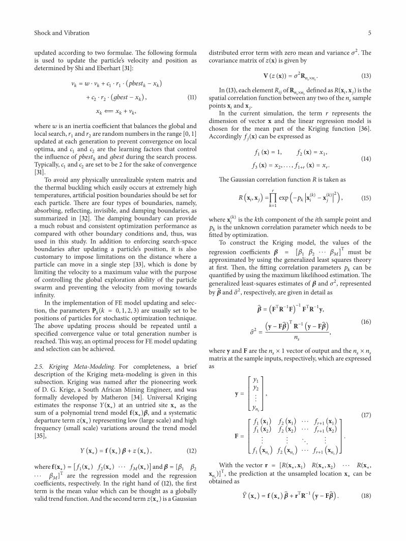
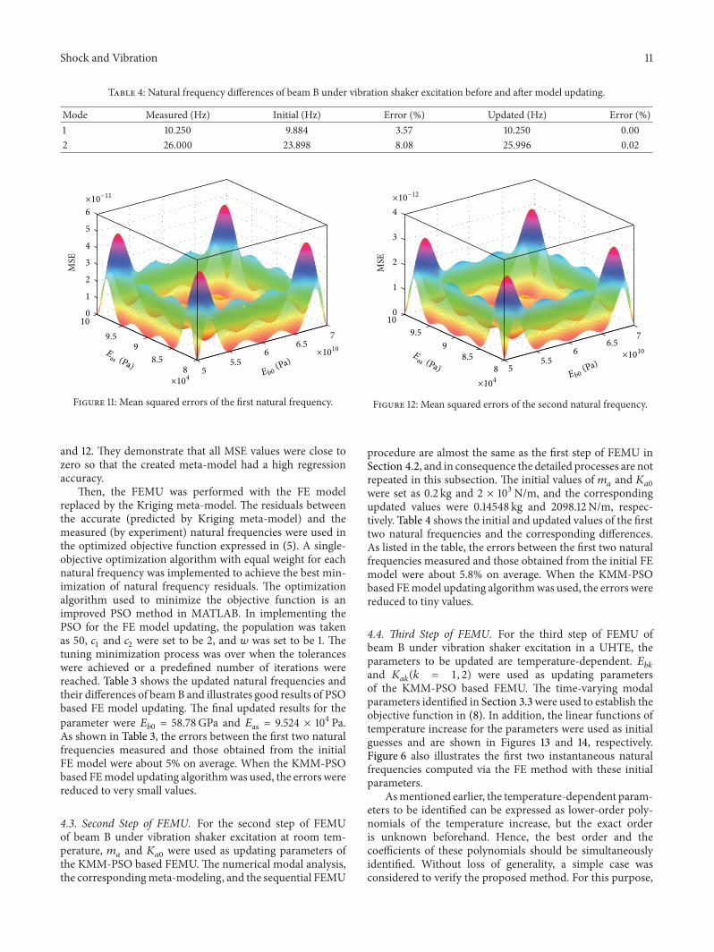

International Journal of
AerospaceEngineeringHindawi Publishing Corporationhttpwwwhindawicom Volume 2014
RoboticsJournal of
Hindawi Publishing Corporationhttpwwwhindawicom Volume 2014
Hindawi Publishing Corporationhttpwwwhindawicom Volume 2014
Active and Passive Electronic Components
Control Scienceand Engineering
Journal of
Hindawi Publishing Corporationhttpwwwhindawicom Volume 2014
International Journal of
RotatingMachinery
Hindawi Publishing Corporationhttpwwwhindawicom Volume 2014
Hindawi Publishing Corporation httpwwwhindawicom
Journal ofEngineeringVolume 2014
Submit your manuscripts athttpwwwhindawicom
VLSI Design
Hindawi Publishing Corporationhttpwwwhindawicom Volume 2014
Hindawi Publishing Corporationhttpwwwhindawicom Volume 2014
Shock and Vibration
Hindawi Publishing Corporationhttpwwwhindawicom Volume 2014
Civil EngineeringAdvances in
Acoustics and VibrationAdvances in
Hindawi Publishing Corporationhttpwwwhindawicom Volume 2014
Hindawi Publishing Corporationhttpwwwhindawicom Volume 2014
Electrical and Computer Engineering
Journal of
Advances inOptoElectronics
Hindawi Publishing Corporation httpwwwhindawicom
Volume 2014
The Scientific World JournalHindawi Publishing Corporation httpwwwhindawicom Volume 2014
SensorsJournal of
Hindawi Publishing Corporationhttpwwwhindawicom Volume 2014
Modelling amp Simulation in EngineeringHindawi Publishing Corporation httpwwwhindawicom Volume 2014
Hindawi Publishing Corporationhttpwwwhindawicom Volume 2014
Chemical EngineeringInternational Journal of Antennas and
Propagation
International Journal of
Hindawi Publishing Corporationhttpwwwhindawicom Volume 2014
Hindawi Publishing Corporationhttpwwwhindawicom Volume 2014
Navigation and Observation
International Journal of
Hindawi Publishing Corporationhttpwwwhindawicom Volume 2014
DistributedSensor Networks
International Journal of