Sensors & Transducers, Vol. 166, Issue 3, March 2014, pp. 163-172

163

SSSeeennnsssooorrrsss &&& TTTrrraaannnsssddduuuccceeerrrsss

© 2014 by IFSA Publishing, S. L. http://www.sensorsportal.com

Research on Optimal Scheduling Period of Flexray Based on Jitter-free Transmission

1, 2 Zhipeng GONG, 1 Tefang CHEN, 3 Fumin ZOU, 2 Xilong QU

and 4 Zhongxiao HAO 1 School of Information Science and Engineering, Central South University,

Changsha, 410083, China 2 College of Electrical and Information Engineering,

Hunan Institute of engineering, Xiangtan, 411104, China 3 School of Information Science and Engineering,

Fujian University of Technology, Fuzhou, 350108, China 4 School of Information Science & Electrical Engineering, Hebei University of Engineering, Handan, 056038, China

1 Tel. :+( 86)-731-58688937 E-mail:zpgong2000@126.com

Received: 18 December 2013 /Accepted: 28 February 2014 /Published: 31 March 2014 Abstract: The scheduling period (SP) is an important parameter for building an in-vehicle communication network based on FlexRay bus. In this paper, we analyze the impact of SP on the bus bandwidth utilization and transmission jitter, study the method of assignment of bus period with jitter constraints, investigate necessary conditions should be meet when jitter-free transmission is demanded and establish mathematical model for the optimal SP. Considering there are many long period messages on in-vehicle communication network and much of bandwidth is wasted by them, we put forward an integer period extended model (IPEM) and present the structure of the modified period scheduling table and corresponding software architecture as well, thus the long period message can be transmitted with a period larger than SP and the bandwidth demanded is reduced dramatically. At last, the model is verified by various kinds of message sets and the result of simulation indicates that our method is effective. Copyright © 2014 IFSA Publishing, S. L. Keywords: Jitter, FlexRay, Period assignment, In-vehicle, Communication network. 1. Introduction 1.1. FlexRay and In-Vehicle

Communication Network

Due to the excellent performance, FlexRay is attracting increasing attention and expected to be the standard in-vehicle communication network of the next generation. Because of its broad bandwidth, high

determinacy, high performance of fault tolerance and the outstanding topological flexibility, FlexRay is qualified for increasingly complex electronic electrical architecture (EEA) design of modern automotive based on x-by-wire technology with high security, high reliability and strong real-time property [1, 2].

FlexRay was raised by Daimler-Chrysler Corporation in 1999, and has been maintained by the

Article number P_1920

Sensors & Transducers, Vol. 166, Issue 3, March 2014, pp. 163-172

164

FlexRay consortium after that. FlexRay consortium is comprised of more than 120 members, including almost all of automotive industry related international companies, such as Daimler-Chrysler, BMW, AUDI, FREESCALE, NXP, etc. Up to now, significant progress in application fields of FlexRay bus has been made: 1) The release of FlexRay IP core. In 2004, BOSCH released the first IP core of communication controller (CC) compatible with FlexRay protocol specification known as E-Ray, before long, like product was also developed by IPextreme known as FRCC2100; 2) The appearance of silicon chip of CC on the market. Manufacturers integrated CC IP as a peripheral device into their microprocessor chip or made a separated ASIC with the IP, such as MC9S12XF512 and MFR4300; 3) The successful development of FlexRay bus driver (BD). In 2006, NXP successfully developed the first FlexRay transceiver JTA1080 and it declares the process of FlexRay development has stepped into the application stage. In 2010, road vehicle communication specification based on FlexRay was officially adopted by the international standard as ISO10681 [3], which marks the internationalization of FlexRay has made great progress. At the same time, AUTOSAR4.0 also provided support for FlexRay and had drafted corresponding standards of software architecture design for transport layer and network management layer [4]. FlexRay is becoming an international in-vehicle communication network.

FlexRay is actually derived from TTP [5] and BYTEFLIGHT, and has the merits of both time-triggered network and event-triggered network [6]. The access of node to FlexRay bus is realized through repetitive communication cycle known as FlexRay cycle (FC), which is composed of static segment (SS), dynamic segment (DS), symbol window (SW) and network idle time (NIT) [7], and data transmission is carried out on SS and DS. The SS is responsible for the transmission of periodic real-time messages. In order to guarantee the deterministic network transmission, the SS employs the media access control based on time division multiple access (TDMA). The SS is divided into many slots of equal time, and in each slot, the transmission of a static frame is executed. The DS is designed for the transmission of sporadic real-time messages. In order to improve the transmission efficiency, the DS use access control based on flexible time division multiple access (FTDMA).

1.2. Problem Description

Indubitably, flexray has showed outstanding virtues and attractive prospects, nevertheless, its drawbacks are also obvious, e.g., the protocol of FlexRay is bulky and complex, the node of electronic control unit (ECU) is very hard to join in a FlexRay network, message scheduling is pretty difficult, and a distributed embedded system based on flexray is hard to extend. These problems have seriously hindered the further popularization of FlexRay. For the

realization of “once installed correctly, the system would work steadily”, at the beginning of construction of the FlexRay network, most relevant parameters must be predetermined. We'll discuss how to determine the parameter of scheduling period (SP) in this paper.

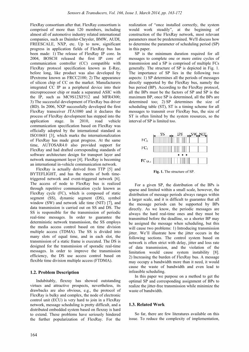
SP is the minimum duration required for all messages to complete one or more entire cycles of transmission and a SP is comprised of multiple FCs generally. The structure of SP is depicted in Fig. 1. The importance of SP lies in the following two aspects: 1) SP determines all the periods of messages directly supported by the FlexRay bus, namely the bus period (BP). According to the FlexRay protocol, all the BPs must be the factors of SP and SP is the maximum BP, once SP is determined, all the BPs are determined too; 2) SP determines the size of scheduling table (ST), ST is a timing scheme for all messages to transmit over FlexRay bus, the size of ST is often limited by the system resources, so the interval of SP is limited too.

Fig. 1. The structure of SP.

For a given SP, the distribution of the BPs is sparse and limited within a small scale, however, the distribution of message periods always ranges within a larger scale, and it is difficult to guarantee that all the message periods can be supported by BPs directly. As we know, the periodic messages are always the hard real-time ones and they must be transmitted before the deadline, so a shorter BP may be assigned the message when scheduling, but this will cause two problems: 1) Introducing transmission jitter. We’ll illustrate how the jitter occurs in the following sections. The control system based on network is often strict with delay, jitter and loss rate of data transmission, and the violation of the limitation would cause system instability [8]. 2) Increasing the burden of FlexRay bus. A message may occupy a bandwidth more than it need, it would cause the waste of bandwidth and even lead to infeasible scheduling.

In this paper we purpose on a method to get the optimal SP and corresponding assignment of BPs to realize the jitter-free transmission while minimize the waste of bandwidth. 1.3. Related Work

So far, there are few literatures available on this issue. To reduce the complexity of implementation,

Sensors & Transducers, Vol. 166, Issue 3, March 2014, pp. 163-172

165

some standards specifications employ the principle of simple periodic system [9]. For example, in AUTOSAR specification, FlexRay bus period is designated as 2n, i.e., the BP is fixed at 2, 4, 8… the engineer is required to decide the message period from view of the support provided by system. Simple periodic system has the advantage of easiness of implementation, but may degrade system performance. In order to cope with the complicated message of general period distribution, we should find a solution to get the optimal SP. As to the scenario when the distribution of message period and SP are given, Klaus Schmidt proposed the optimal scheduling algorithm based on number theory [10].

1.4. Arrangement of This Paper

The structure of this paper is presented as follows. In Section 2, we discuss the FlexRay transmission jitter, analyze jitter in the worst case and summarize scheduling conditions for jitter-free transmission, then determine the performance metrics and set up the programming model. In Section 3, we survey the problem of bandwidth utilization occurs during the scheduling of long period messages and put forward an improved solution, namely, the integer period extended model (IPEM) and present corresponding software design architecture. Section 4 presents the result of simulation. Conclusions are given in Section 5.

2. Model and Solution 2.1. Conditions and Assumptions

There is no problem of jitter with the DS, so this paper mainly considers the scheduling of periodic real-time message on the SS. We assume that there is only one channel employed, the periodic message of the SS constitute a set M = {m1, m2,... mN}, the property kmi of i'th message mi is characterized by a triple ( pmi, dmi, emi ) with period pmi, deadline dmi and transmission times emi. For the sake of simplicity, we assume that the data has been packaged into messages, the length of the SS frame has been pre-calculated already, all the transmission time of messages are identical and set to one unit, i.e., emi =1. We also assume that dmi= emi. Let BPS denote the ordered set of BPs, i.e., BPS={bp1,bp2,…bpK}, where bpi<bpi+1, According to the FlexRay protocol, all the elements of BPS must be the factors of SP. Assuming function factor (n) is used to get all the factors of n, including factor 1, so BPS=factor(SP), We also assume the maximum SP permitted for the FlexRay bus is SP_MAX FCs. 2.2. Transmission Jitter

Definition 1: Transmission Jitter ( jit ). We denote the period of message m by pm, the bus period

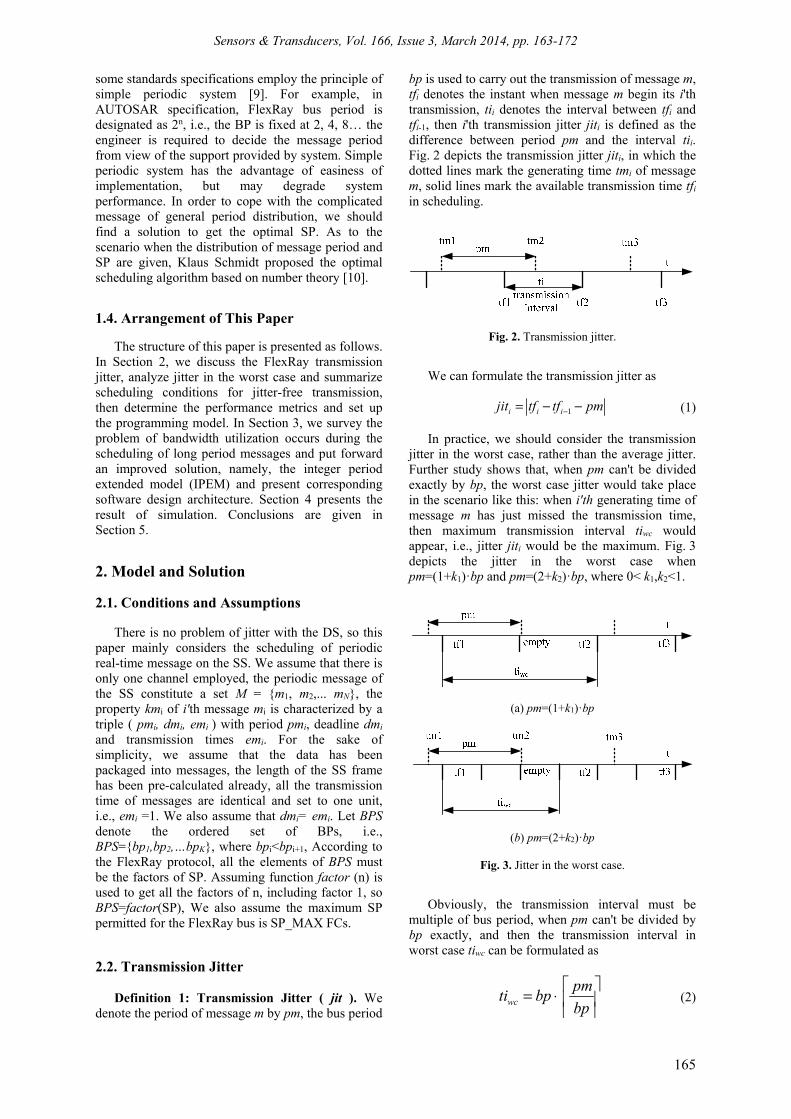
bp is used to carry out the transmission of message m, tfi denotes the instant when message m begin its i'th transmission, tii denotes the interval between tfi and tfi-1, then i'th transmission jitter jiti is defined as the difference between period pm and the interval tii. Fig. 2 depicts the transmission jitter jiti, in which the dotted lines mark the generating time tmi of message m, solid lines mark the available transmission time tfi in scheduling.

Fig. 2. Transmission jitter.

We can formulate the transmission jitter as

1i i ijit tf tf pm−= − − (1)

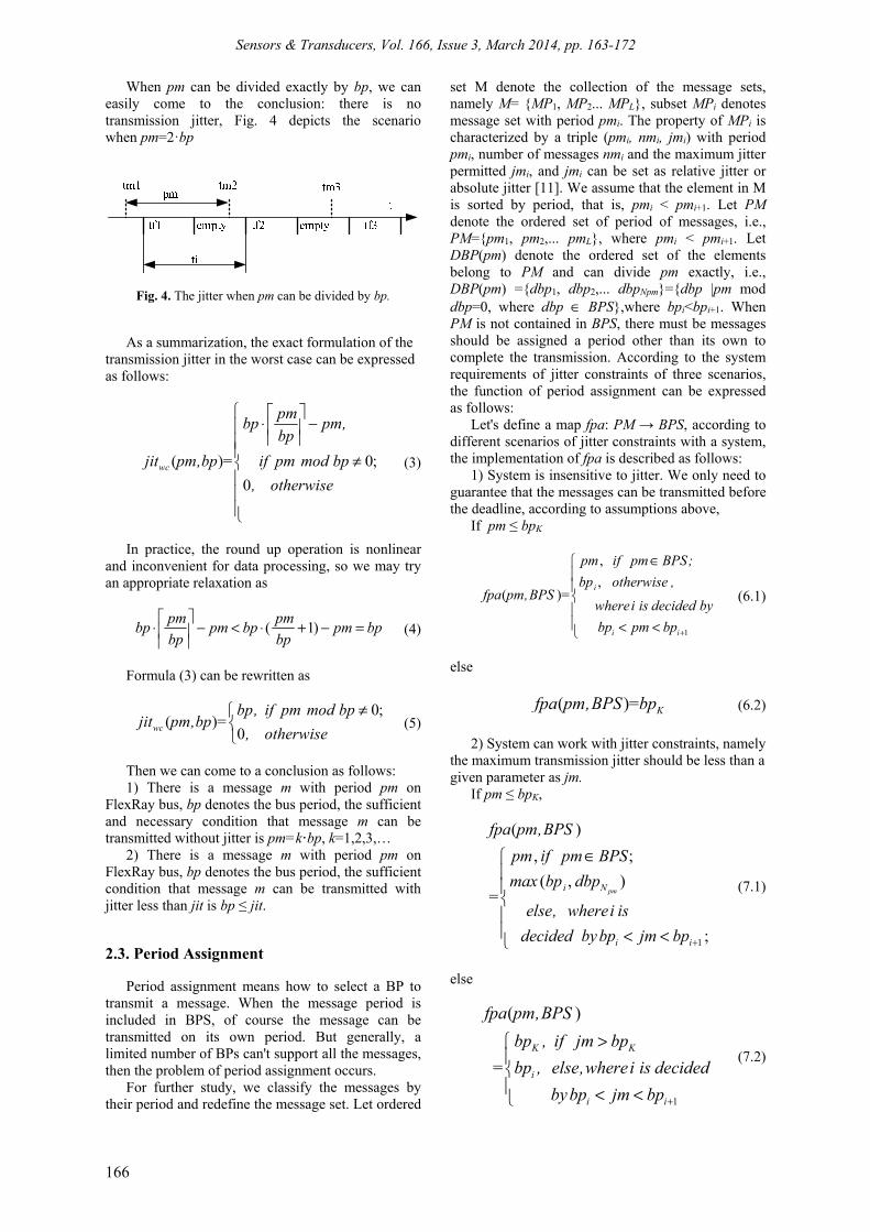
In practice, we should consider the transmission jitter in the worst case, rather than the average jitter. Further study shows that, when pm can't be divided exactly by bp, the worst case jitter would take place in the scenario like this: when i'th generating time of message m has just missed the transmission time, then maximum transmission interval tiwc would appear, i.e., jitter jiti would be the maximum. Fig. 3 depicts the jitter in the worst case when pm=(1+k1)·bp and pm=(2+k2)·bp, where 0< k1,k2<1.

(a) pm=(1+k1)·bp

(b) pm=(2+k2)·bp

Fig. 3. Jitter in the worst case.

Obviously, the transmission interval must be multiple of bus period, when pm can't be divided by bp exactly, and then the transmission interval in worst case tiwc can be formulated as

wc

pmti bp

bp

= ⋅

(2)

Sensors & Transducers, Vol. 166, Issue 3, March 2014, pp. 163-172

166

When pm can be divided exactly by bp, we can easily come to the conclusion: there is no transmission jitter, Fig. 4 depicts the scenario when pm=2·bp

Fig. 4. The jitter when pm can be divided by bp.

As a summarization, the exact formulation of the transmission jitter in the worst case can be expressed as follows:

( )= 0;

0wc

pmbp pm,

bp

jit pm,bp if pm mod bp

, otherwise

⋅ − ≠

(3)

In practice, the round up operation is nonlinear

and inconvenient for data processing, so we may try an appropriate relaxation as

( 1)

pm pmbp pm bp pm bp

bp bp

⋅ − < ⋅ + − =

(4)

Formula (3) can be rewritten as

0;

( )=0wc

bp, if pm mod bpjit pm,bp

, otherwise

≠

(5)

Then we can come to a conclusion as follows: 1) There is a message m with period pm on

FlexRay bus, bp denotes the bus period, the sufficient and necessary condition that message m can be transmitted without jitter is pm=k·bp, k=1,2,3,…

2) There is a message m with period pm on FlexRay bus, bp denotes the bus period, the sufficient condition that message m can be transmitted with jitter less than jit is bp ≤ jit. 2.3. Period Assignment

Period assignment means how to select a BP to transmit a message. When the message period is included in BPS, of course the message can be transmitted on its own period. But generally, a limited number of BPs can't support all the messages, then the problem of period assignment occurs.

For further study, we classify the messages by their period and redefine the message set. Let ordered

set M denote the collection of the message sets, namely M= {MP1, MP2... MPL}, subset MPi denotes message set with period pmi. The property of MPi is characterized by a triple (pmi, nmi, jmi) with period pmi, number of messages nmi and the maximum jitter permitted jmi, and jmi can be set as relative jitter or absolute jitter [11]. We assume that the element in M is sorted by period, that is, pmi < pmi+1. Let PM denote the ordered set of period of messages, i.e., PM={pm1, pm2,... pmL}, where pmi < pmi+1. Let DBP(pm) denote the ordered set of the elements belong to PM and can divide pm exactly, i.e., DBP(pm) ={dbp1, dbp2,... dbpNpm}={dbp |pm mod dbp=0, where dbp ∈ BPS},where bpi<bpi+1. When PM is not contained in BPS, there must be messages should be assigned a period other than its own to complete the transmission. According to the system requirements of jitter constraints of three scenarios, the function of period assignment can be expressed as follows:

Let's define a map fpa: PM → BPS, according to different scenarios of jitter constraints with a system, the implementation of fpa is described as follows:

1) System is insensitive to jitter. We only need to guarantee that the messages can be transmitted before the deadline, according to assumptions above,

If pm ≤ bpK

1

,

,( )=

+

∈ < <

i

i i

pm if pm BPS;

bp otherwise ,fpa pm,BPS

wherei is decided by

bp pm bp

(6.1)

else

( )= Kfpa pm,BPS bp (6.2)

2) System can work with jitter constraints, namely

the maximum transmission jitter should be less than a given parameter as jm.

If pm ≤ bpK,

1

( )

, ;

( , )=

;+

∈ < <

pmi N

i i

fpa pm,BPS

pm if pm BPS

max bp dbp

else, wherei is

decided bybp jm bp

(7.1)

else

1

( )

=K K

i

i i

fpa pm,BPS

bp , if jm bp

bp , else,wherei is decided

bybp jm bp +

> < <

(7.2)

Sensors & Transducers, Vol. 166, Issue 3, March 2014, pp. 163-172

167

3) system can’t work with any jitter, according to formula (5)

( )=pmNfpa pm,BPS dbp (8)

2.4. Performance Metrics and Optimal Model

After the period assignment, we need to determine the optimal bus period distribution, i.e., to determine the parameters of FC and SP. In general, FC and SP can be calculated as follows [12]:

FC=gcd ( pm1, pm2,... , pmL), SP=lcm ( pm1, pm2,... , pmL ),

There is no problem with FC determined by this

means, but as for SP, it is a different matter. According to the FlexRay protocol, SP may be composed of SP_MAX FCs at most, but SP determined by this manner is likely larger than SP_MAX, so we have to find the optimal SP.

Let's consider message set MP with period pm, number of messages nm and length of messages length, assume the rate of FlexRay bus is B bps. Then the fraction of the FlexRay bandwidth B that is originally demanded by MP is

MP

length nmBM

pm FC B

⋅=⋅ ⋅

(9)

For the sake of convenience, we use the item

bandwidth to imply the fraction of the FlexRay bandwidth B, According to the period assignment function above, the bandwidth allocated for MP is

( , )MP

length nmBS

fpa pm BPS FC B

⋅=⋅ ⋅

(10)

Bandwidth demanded by all the messages

amounts to

i i

iM MPi

MP MP i

length nmBM BM

pm FC B

⋅= =⋅ ⋅ (11)

Similarly, the bandwidth allocated for all the

messages is

( , )

=⋅=

⋅ ⋅ i

i i

M

iMP

MP MP i

BS

length nmBS

fpa pm BPS FC B

(12)

The bandwidth utilization R illustrates how much

of the allocated bandwidth is used for messages transmission, which is given by

( , )

( , )

i

i

i

i

i

MP iM

iM

MP i

i

MP i

i

MP i

length nm

pm FC BBMR

length nmBSfpa pm BPS FC B

nm

pmnm

fpa pm BPS

⋅⋅ ⋅

= = ⋅⋅ ⋅

=

(13)

If we ignore the consequent FID assignment here,

our objective is to choose an appropriate SP to maximum the bandwidth utilization R. Considering the required bandwidth BM of a given message set M is fixed, our objective is converted to minimum the bandwidth allocated to the message set. Let SPS denote the set of potential SPs, the mathematical programming model is

. .

(SP)

(6) ~ (8)

:

( , )

M MPiSP SPS MPi M

iMPi

i

y BS BSmin

s t

BPS factor

formula

MPi M

length nmB

fpa pm BPS FC B

∈ ∈

= =

=

∀ ∈⋅=

⋅ ⋅

(14)

Specially, for jitter-free transmission, the model

can be transformed into the BIP. we assume function prime (n) is used to get the set of all prime factors of n; let FMSi denote the ordered set of all prime factors of period pmi in message set MPi, let Qi denote the number of prime factor of pmi, i.e., FMSi =prime (pmi) ={fmsi, 1, fmsi, 2,... fmsi, Qi}, where fmsi, j ≤ fmsi, j+1, and two identical factors represent different elements respectively. Suppose SP is set to 1 initially. If factor fmsi,j is selected, the bandwidth allocated to MPi will be reduced to 1/ fmsi, j, but the product of all selected factors must be less than SP_MAX. i.e., SP≤ SP_MAX. Let vector Xi= [xi,1, xi,2, xi,3... xi,Qi] denote the variable to decide whether factor fmsi,j is selected or not, if xi,j=1, fmsi,j is selected, otherwise fmsi j is not selected. Let FS denote the set of all prime factors, i.e., FS= {fs1, fs2... fsH}. Let vector X=[x1, x2, x3,... , xH] denote the variable to decide whether factor fsi is selected or not, if xi=1, fsi is selected, otherwise fsi is not selected. Obviously, all the elements in FMSi are included in FS. Let's define a map w: Xi→ X as

w(xi,j)=xh, if fmsi, j=fsh.

The mathematical model (we call it the original

optimal model here) can be rewritten as

Sensors & Transducers, Vol. 166, Issue 3, March 2014, pp. 163-172

168

,,

,

. .

(1 ( 1) ) _

:

( )

1(1 ( ))

∈

∈

=

= + − ≤

∀ ∈=

=

−⋅ ⋅ − ⋅

⋅

∏

∏

i

i

i

i

i

MPX MP M

i ifs FS

i

i i

MP

i ji i j

FMS i j

y BSmin

s t

SP fs x SP MAX

MP M

FMS prime pm

B

fmslengthnm w x

FC B fms

, (15)

we can use the MINLP solver of TOMLAB tool to solve this problem [13]

Let MPIi denote the messages during interval of [bpi, bpi+1]. If there is no jitter constraint, we can calculate the extra bandwidth caused by period assignment as

1

1 1( )

= ( )

∈ ∈

∈ ∈ =

=

⋅ ⋅ −⋅

⋅ −⋅

jj i

i jj

EX

ibp BPS pm i i

Li i

bp BPS pm i

MPI

iMPI i

B

lengthnm

FC B bp pm

nm nmlength

FC B bp pm

(16)

As a further step, we assume that the messages

follow a uniform distribution of number against period with density set to 1, and then the extra bandwidth is

1 1

1 1( )

1= ( )

j i j

EXbp BPS pm MPI i i

K Li

i ii i

lengthB

FC B bp pm

llength

FC B bp pm

∈ ∈

= =

= ⋅ −⋅

⋅ −⋅

(17)

3. Improved Model 3.1. Drawback of Original optimal model

In original optimal model, a message with period larger than SP would have to transmit with a BP shorter than its own (SP at most), even if the period of message is much larger than SP. For the sake of convenience, we use the term LPM to represent the message with period larger than SP. In fact, there are always a large number of LPMs in a system in practice. e.g., among the messages in-vehicle confirmed by surface vehicle standard J1939 [14], if SP=64 FCs, Almost half of messages are LPMs. If original optimal model is employed, the LPMs would transmit with a BP much shorter than the message period, which would cause the waste of bandwidth, In order to solve this problem, we put forward two solutions as follows.

1) Multiple Scheduling Table Model (MSTM). The FlexRay transmission is composed of an infinite loop in fact and message of any period can be transmitted without jitter theoretically. To realize the jitter-free transmission, all the related nodes, including source nodes and the target nodes, should keep a counter modulo the message period, i.e., we have to build a ST for every message individually. If a node has many periodic messages to transmit over FlexRay bus, it has to maintain multiple STs for these messages. It is the multiple scheduling tables model (MSTM). In MSTM, all messages, including LPMs can realize the jitter-free transmission without extra bandwidth demand. But its defects are also apparent: 1) different kind of message may need different ST. When a node needs to deal with a variety of messages, it has to maintain many STs. Take the system monitoring node for example, it may need all kinds of messages, so it would have to keep so many STs. which would consume a large amount of system resources, such as memory space and CPU time; 2) MSTM is hard to maintain when there are too many STs, it may cause the scheduling chaos, for example, once a message is scheduled in wrong time, conflict may occur and the error is hard to correct.

2) Integer Period Extended Model (IPEM). In order to reduce the maintenance of ST while the utilization of FlexRay bus can be kept at a reasonable level, we only modify the period assignment of LPMs and enable LPMs to transmit with the period of multiple of SP, to achieve this, we build up corresponding circumstance for transmission. In IPEM, only one ST is needed. The field of FC counter in the preamble of frame is still in use, this lightens node the burden of maintaining of ST. IPEM will be described in detail in the following parts 3.2. The Condition of IPEM

Not all situations are suitable for IPEM, before extension of period, there are several conditions as follows should be meet: 1) the period of LPM must be the multiple of SP, 2) or the period of LPM can be adjusted to the multiple of SP (usually adjusted downward); 3) there are enough LPMs, because IPEM may consume some resources itself, it is not worthwhile to employ IPEM for too few messages. 3.3. The Implementation of IPEM

The implementation of IPEM is described as follows: 1) Get the optimal SP by solving the programming model in section 2; 2) Adjust the period of LPMs when necessary, according to requirement for the period extension; 3) Add a network service frame (NSF) into the ST to track the count of SP. We denote the counter of SP by nSP and it can be set as a network management vector in application. The NSF is located at the first slot of the first FC in ST for the convenience of the operation of

Sensors & Transducers, Vol. 166, Issue 3, March 2014, pp. 163-172

169

related nodes; 4) Calculate the global FC count (gFC). During the transmission of LPMs, the LPMs related nodes have to keep the track of count of current FC based on the modulus of max extended period, let nFC denote the FC count in the preamble. We can formulate the gFC as

gFC nSP SP nFC= ⋅ + (18)

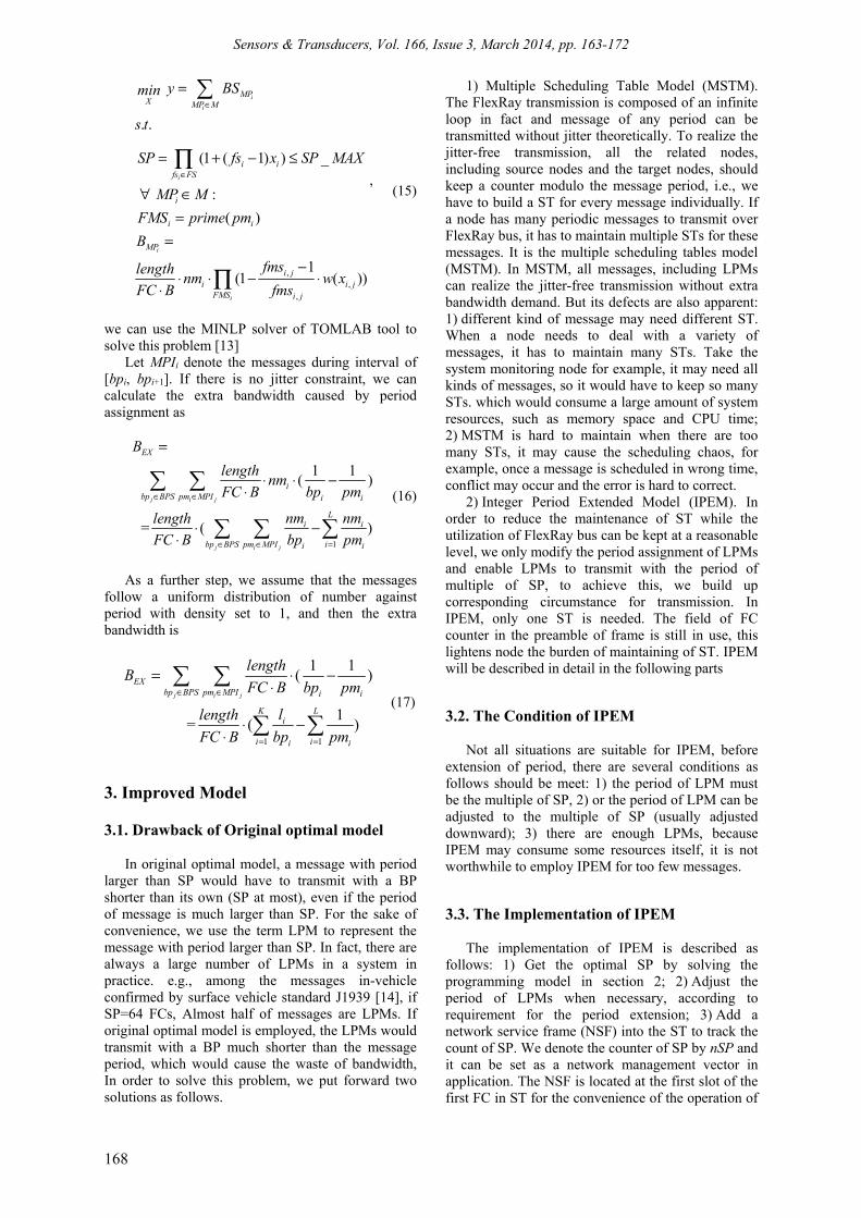
NSF can be maintained by a synchronization node, this node keeps a counter on the SP and NSF should be sent every SP. NSF would occupy some bandwidth itself, but it is negligible when there are a large number LPMs, at the same time, NSF can be used to complete other services related with the bus management, of course, NSF can also be used to transmit messages. Structure of ST based on IPEM is depicted in Fig. 5.

Fig. 5. Scheduling table of IPEM.

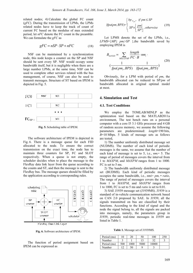
The software architecture of IPEM is depicted in Fig. 6. There is a message queue for each FID allocated to the node. To ensure the correct transmission on the exact time, the node has to maintain three counters for SP, FC and SLOT respectively. When a queue is not empty, the scheduler decides when to place the message to the FlexRay data link layer from the queue according to the counts and ST, and then the message is sent to the FlexRay bus. The message queues should be filled by the application according to corresponding rules.

Fig. 6. Software architecture of IPEM.

The function of period assignment based on IPEM can be expressed as

,

( )=

≤ ×

pmNbp if pm SP

lfpa pm,BPS pmSP ,otherwise

SP

(19)

Let LPMS denote the set of the LPMs, i.e., LPMS={MPi| pmi>SP },the bandwidth saved by employing IPEM is

1 1( )

( , ) ( , )

∈

= ⋅ ⋅⋅

−

i

SAVED iMP LPMP

i i

lengthB nm

FC B

fpa pm BPS lfpa pm BPS

(20)

Obviously, for a LPM with period of pm, the

bandwidth allocated can be reduced to SP/pm of bandwidth allocated in original optimal model at most.

4. Simulation and Test 4.1. Test Conditions

We employ the TOMLAB/MINLP as the optimization tool based on the MATLAB2011a environment, The test bench runs on a personal computer with a core I5 3.1 GHz processor and 4 GB of random access memory, we assume the following parameters are predetermined: length=190 bits, B=10 Mbps. 5 kinds of message sets as follows are tested,

1) The number uniformly distributed message set (NUDMS). The number of each kind of periodic messages is the same, we assume that the number of each kind of message is set to 5, i.e., nmi= 5. The range of period of messages covers the interval from 1 to MAXPM, and MAXPM ranges from 1 to 1000. FC is set to 5 ms.

2) The bandwidth uniformly distributed message set (BUDMS). Each kind of periodic messages occupies the same bandwidth, i.e., nmi= pmi • ratio, The range of period of messages covers the interval from 1 to MAXPM, and MAXPM ranges from 1 to 1000, FC is set to 5 ms and ratio is set to 0.01.

3) SAE J1939 message set (J1939MS). J1939 is a standard of in-vehicle communication network based on CAN 2.0 proposed by SAE. In J1939, all the signals transmitted on bus are classified by their functions. According to the kind of signal and the node the signal belong to, all the signals are packed into messages, namely, the parameters group in J1939, periodic real-time messages in J1939 are listed in Table 1.

Table 1. Message set of J1939MS.

Period (ms) 10 20 50 100 250 Number 3 1 13 32 3 Period (ms) 500 1000 5000 10000 Number 12 50 9 3

Sensors & Transducers, Vol. 166, Issue 3, March 2014, pp. 163-172

170

4) Extended SAE J1939 message set (EJ1939MS). Considering the CAN runs at 1 Mbps at most, in order to test the performance of our algorithm more exactly, we create a message set based on the extension of J1939, which is shown in Table 2.

Table 2. Message set of EJ1939MS.

Period (ms) 1 2 5 10 20 50 Number 3 3 3 3 1 13 Period (ms) 100 250 500 1000 5000 10000 Number 32 3 12 50 9 3

5) SAE message set (SAEMS). This message set is specialized for test of in-vehicle communications by SAE[15], there are the 51 messages in it, which is listed in Table 3.

Table3. Message set of SAEMS.

Period (ms) 5 10 20 100 1000 Number 9 2 30 6 6

4.2. Test Result and Analysis

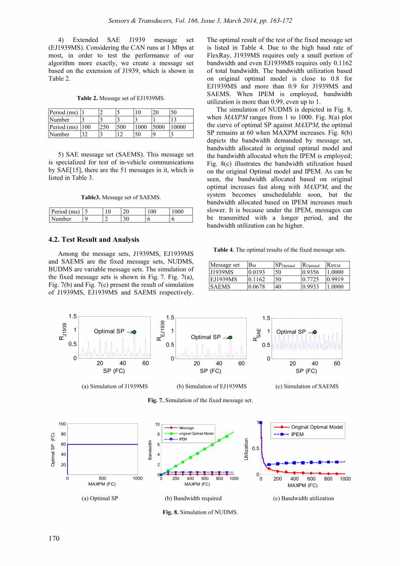
Among the message sets, J1939MS, EJ1939MS and SAEMS are the fixed message sets, NUDMS, BUDMS are variable message sets. The simulation of the fixed message sets is shown in Fig. 7. Fig. 7(a), Fig. 7(b) and Fig. 7(c) present the result of simulation of J1939MS, EJ1939MS and SAEMS respectively.

The optimal result of the test of the fixed message set is listed in Table 4. Due to the high baud rate of FlexRay, J1939MS requires only a small portion of bandwidth and even EJ1939MS requires only 0.1162 of total bandwidth. The bandwidth utilization based on original optimal model is close to 0.8 for EJ1939MS and more than 0.9 for J1939MS and SAEMS. When IPEM is employed, bandwidth utilization is more than 0.99, even up to 1.

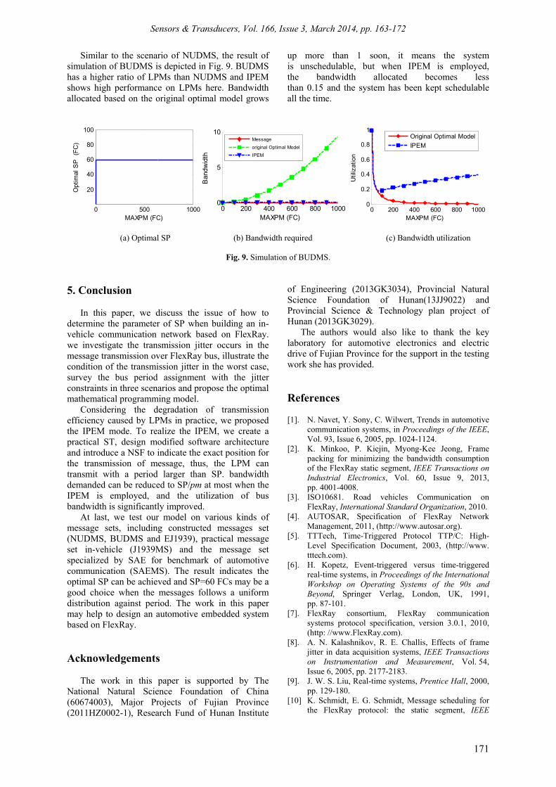
The simulation of NUDMS is depicted in Fig. 8, when MAXPM ranges from 1 to 1000. Fig. 8(a) plot the curve of optimal SP against MAXPM, the optimal SP remains at 60 when MAXPM increases. Fig. 8(b) depicts the bandwidth demanded by message set, bandwidth allocated in original optimal model and the bandwidth allocated when the IPEM is employed; Fig. 8(c) illustrates the bandwidth utilization based on the original Optimal model and IPEM. As can be seen, the bandwidth allocated based on original optimal increases fast along with MAXPM, and the system becomes unschedulable soon, but the bandwidth allocated based on IPEM increases much slower. It is because under the IPEM, messages can be transmitted with a longer period, and the bandwidth utilization can be higher.

Table 4. The optimal results of the fixed message sets.

Message set BM SPOptimal ROptimal RIPEM J1939MS 0.0193 50 0.9356 1.0000 EJ1939MS 0.1162 50 0.7725 0.9919 SAEMS 0.0678 40 0.9933 1.0000

20 40 600

0.5

1

1.5

SP (FC)

R J193

9

Optimal SP →

20 40 600

0.5

1

1.5

SP (FC)

REJ

1939

Optimal SP →

20 40 600

0.5

1

1.5

SP (FC)

R SAE Optimal SP →

(a) Simulation of J1939MS (b) Simulation of EJ1939MS (c) Simulation of SAEMS

Fig. 7. Simulation of the fixed message set.

0 500 1000

20

40

60

80

100

MAXPM (FC)

Opt

imal

SP

(FC

)

0 200 400 600 800 1000

0

2

4

6

8

10

MAXPM (FC)

Ban

dwid

th

Messageoriginal Optimal ModelIPEM

0 200 400 600 800 1000

0

0.5

1

MAXPM (FC)

Util

izat

ion

Original Optimal ModelIPEM

(a) Optimal SP (b) Bandwidth required (c) Bandwidth utilization

Fig. 8. Simulation of NUDMS.

Sensors & Transducers, Vol. 166, Issue 3, March 2014, pp. 163-172

171

Similar to the scenario of NUDMS, the result of simulation of BUDMS is depicted in Fig. 9. BUDMS has a higher ratio of LPMs than NUDMS and IPEM shows high performance on LPMs here. Bandwidth allocated based on the original optimal model grows

up more than 1 soon, it means the system is unschedulable, but when IPEM is employed, the bandwidth allocated becomes less than 0.15 and the system has been kept schedulable all the time.

0 500 1000

20

40

60

80

100

MAXPM (FC)

Opt

imal

SP

(FC

)

0 200 400 600 800 10000

5

10

MAXPM (FC)

Ban

dwid

th

Message

original Optimal Model

IPEM

0 200 400 600 800 1000

0

0.2

0.4

0.6

0.8

1

MAXPM (FC)

Util

izat

ion

Original Optimal ModelIPEM

(a) Optimal SP (b) Bandwidth required (c) Bandwidth utilization

Fig. 9. Simulation of BUDMS. 5. Conclusion

In this paper, we discuss the issue of how to determine the parameter of SP when building an in-vehicle communication network based on FlexRay. we investigate the transmission jitter occurs in the message transmission over FlexRay bus, illustrate the condition of the transmission jitter in the worst case, survey the bus period assignment with the jitter constraints in three scenarios and propose the optimal mathematical programming model.

Considering the degradation of transmission efficiency caused by LPMs in practice, we proposed the IPEM mode. To realize the IPEM, we create a practical ST, design modified software architecture and introduce a NSF to indicate the exact position for the transmission of message, thus, the LPM can transmit with a period larger than SP. bandwidth demanded can be reduced to SP/pm at most when the IPEM is employed, and the utilization of bus bandwidth is significantly improved.

At last, we test our model on various kinds of message sets, including constructed messages set (NUDMS, BUDMS and EJ1939), practical message set in-vehicle (J1939MS) and the message set specialized by SAE for benchmark of automotive communication (SAEMS). The result indicates the optimal SP can be achieved and SP=60 FCs may be a good choice when the messages follows a uniform distribution against period. The work in this paper may help to design an automotive embedded system based on FlexRay. Acknowledgements

The work in this paper is supported by The National Natural Science Foundation of China (60674003), Major Projects of Fujian Province (2011HZ0002-1), Research Fund of Hunan Institute

of Engineering (2013GK3034), Provincial Natural Science Foundation of Hunan(13JJ9022) and Provincial Science & Technology plan project of Hunan (2013GK3029).

The authors would also like to thank the key laboratory for automotive electronics and electric drive of Fujian Province for the support in the testing work she has provided. References [1]. N. Navet, Y. Sony, C. Wilwert, Trends in automotive

communication systems, in Proceedings of the IEEE, Vol. 93, Issue 6, 2005, pp. 1024-1124.

[2]. K. Minkoo, P. Kiejin, Myong-Kee Jeong, Frame packing for minimizing the bandwidth consumption of the FlexRay static segment, IEEE Transactions on Industrial Electronics, Vol. 60, Issue 9, 2013, pp. 4001-4008.

[3]. ISO10681. Road vehicles Communication on FlexRay, International Standard Organization, 2010.

[4]. AUTOSAR, Specification of FlexRay Network Management, 2011, (http://www.autosar.org).

[5]. TTTech, Time-Triggered Protocol TTP/C: High-Level Specification Document, 2003, (http://www. tttech.com).

[6]. H. Kopetz, Event-triggered versus time-triggered real-time systems, in Proceedings of the International Workshop on Operating Systems of the 90s and Beyond, Springer Verlag, London, UK, 1991, pp. 87-101.

[7]. FlexRay consortium, FlexRay communication systems protocol specification, version 3.0.1, 2010, (http: //www.FlexRay.com).

[8]. A. N. Kalashnikov, R. E. Challis, Effects of frame jitter in data acquisition systems, IEEE Transactions on Instrumentation and Measurement, Vol. 54, Issue 6, 2005, pp. 2177-2183.

[9]. J. W. S. Liu, Real-time systems, Prentice Hall, 2000, pp. 129-180.

[10] K. Schmidt, E. G. Schmidt, Message scheduling for the FlexRay protocol: the static segment, IEEE

Sensors & Transducers, Vol. 166, Issue 3, March 2014, pp. 163-172

172

Transactions on Vehicular Technology, Vol. 58, Issue 5, 2009, pp. 2170-2179.

[11]. S. D. Vamvakos, V. Stojanovic, B. Nikolic, Discrete-time, linear periodically time-variant phase-locked loop model for jitter analysis, IEEE Transactions on Circuits and Systems, Vol. 58, Issue 6, June 2011, pp. 1211-1224

[12]. E. G. Schmidt, K. Schmidt, Message scheduling for the FlexRay protocol – the dynamic segment, IEEE

Transactions on Vehicular Technology, Vol. 58, Issue 5, 2009, pp. 2160-2169.

[13]. K. Holmstrom, User's guide for tomlab /minlp, 2007, (http://tomopt.com).

[14]. SAE, J1939-71, Vehicle Application Layer, Society of Automotive Engineers SAE, 2001.

[15]. SAE, Class C Application Requirement Considerations, SAE Handbook, Vol. 2, Society of Automotive Engineers SAE, 1994, pp. 366-372.

___________________

2014 Copyright ©, International Frequency Sensor Association (IFSA) Publishing, S. L. All rights reserved. (http://www.sensorsportal.com)