Reservoir simulation_Note01

SIG4042 Reservoir Simulation 2003Lecture note 1

Norwegian University of Science and Technology Professor Jon KleppeDepartment of Petroleum Engineering and Applied Geophysics 14.1.2003

page 1 of 11

INTRODUCTION TO RESERVOIR SIMULATION

Analytical and numerical solutions of simple one-dimensional, one-phase flow equations

As an introduction to reservoir simulation, we will review the simplest one-dimensional flow equations forhorizontal flow of one fluid, and look at analytical and numerical solutions of pressure as function of positionand time. These equations are derived using the continuity equation, Darcy's equation, and compressibilitydefinitions for rock and fluid, assuming constant permeability and viscosity. They are the simplest equations wecan have, which involve transient fluid flow inside the reservoir.

Linear flow

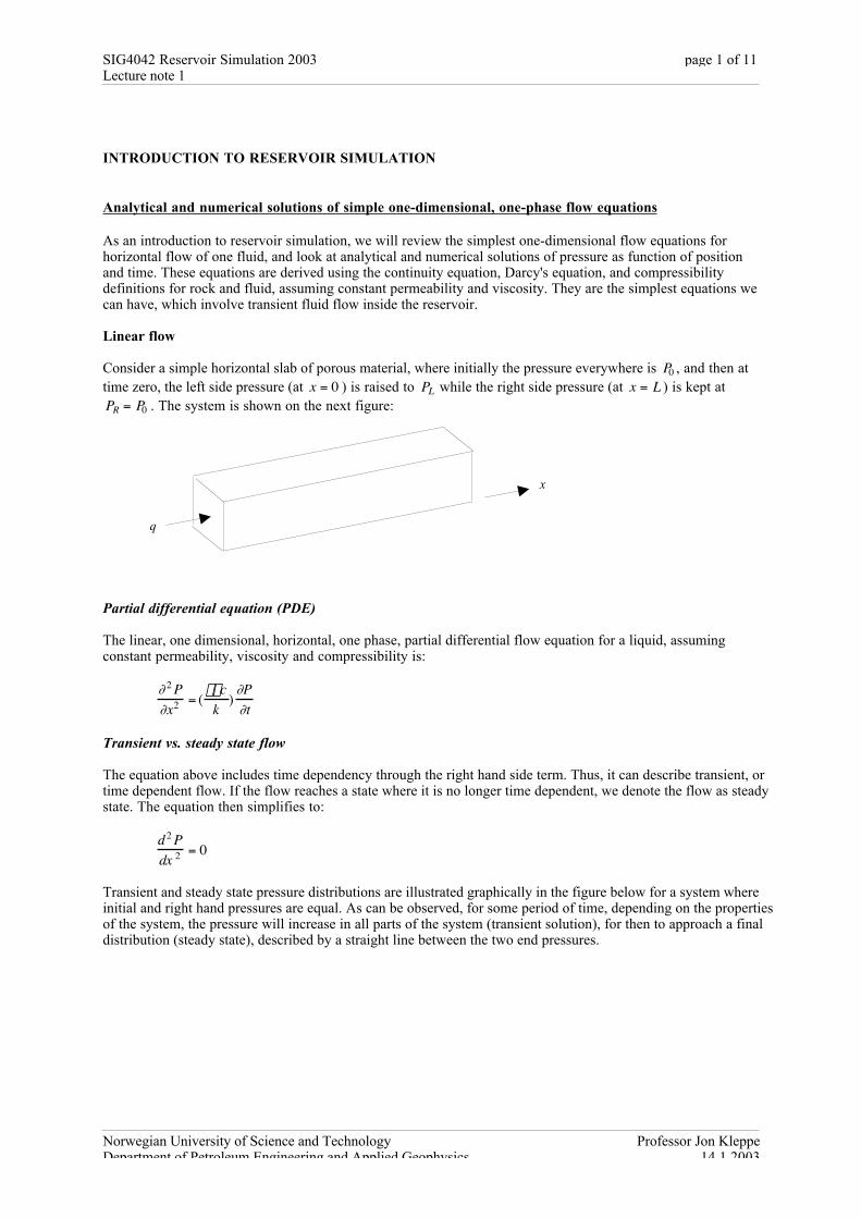
Consider a simple horizontal slab of porous material, where initially the pressure everywhere is P0 , and then attime zero, the left side pressure (at x = 0 ) is raised to PL while the right side pressure (at x = L ) is kept atPR = P0 . The system is shown on the next figure:

Partial differential equation (PDE)

The linear, one dimensional, horizontal, one phase, partial differential flow equation for a liquid, assumingconstant permeability, viscosity and compressibility is:

∂2 P∂x2 = (

fmck

)∂P∂t

Transient vs. steady state flow

The equation above includes time dependency through the right hand side term. Thus, it can describe transient, ortime dependent flow. If the flow reaches a state where it is no longer time dependent, we denote the flow as steadystate. The equation then simplifies to:

d2 Pdx 2 = 0

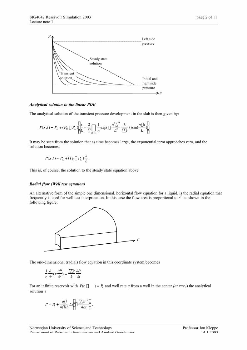
Transient and steady state pressure distributions are illustrated graphically in the figure below for a system whereinitial and right hand pressures are equal. As can be observed, for some period of time, depending on the propertiesof the system, the pressure will increase in all parts of the system (transient solution), for then to approach a finaldistribution (steady state), described by a straight line between the two end pressures.

x

q



page 2 of 11

Analytical solution to the linear PDE

The analytical solution of the transient pressure development in the slab is then given by:

P(x,t ) = PL + (PR - PL )xL

+2p

1n

exp( -n2p 2

L2k

fmct )sin(

npxL

)n =1

•

ÂÈ

Î Í Í

˘

˚ ˙ ˙

It may be seen from the solution that as time becomes large, the exponential term approaches zero, and thesolution becomes:

P(x,t ) = PL + (PR - PL )xL

.

This is, of course, the solution to the steady state equation above.

Radial flow (Well test equation)

An alternative form of the simple one dimensional, horizontal flow equation for a liquid, is the radial equation thatfrequently is used for well test interpretation. In this case the flow area is proportional to r2, as shown in thefollowing figure:

The one-dimensional (radial) flow equation in this coordinate system becomes

1r

∂∂r

(r∂P∂r

) =fmck

∂P∂t

For an infinite reservoir with P(r Æ •) = Pi and well rate q from a well in the center (at r=rw) the analyticalsolution s

P = Pi +qm

4pkhEi -

fmcr 2

4ktÊ

Ë Á

ˆ

¯ ˜ ,

r

P

x

Left sidepressure

Initial andright sidepressure

Steady statesolution

Transientsolution



page 3 of 11

where Ei(-x) = -e-u

ux

•

Ú du is the exponential integral. A steady state solution does not exist for an infinite

system, since the pressure will continue to decrease as long as we produce from the center. However, if we use adifferent set of boundary conditions, so that P(r = rw ) = Pw and P(r = re ) = Pe , we can solve the steady stateform of the equation

1r

ddr

(rdPdr

) = 0

by integration twice, so that the steady state solution becomes

P = Pw +Pe - Pw( )

ln re / rw( )ln r / rw( ) .

Numerical solution

Generally speaking, analytical solutions to reservoir flow equations are only obtainable after making simplifyingassumptions in regard to geometry, properties and boundary conditions that severely restrict the applicability ofthe solution. For most real reservoir fluid flow problems, such simplifications are not valid. Hence, we need tosolve the equations numerically.

Discretization

In the following we will, as a simple example, solve the linear flow equation above numerically by using

standard finite difference approximations for the two derivative terms∂2 P∂x2 and

∂P∂t

. First, the x-coordinate must

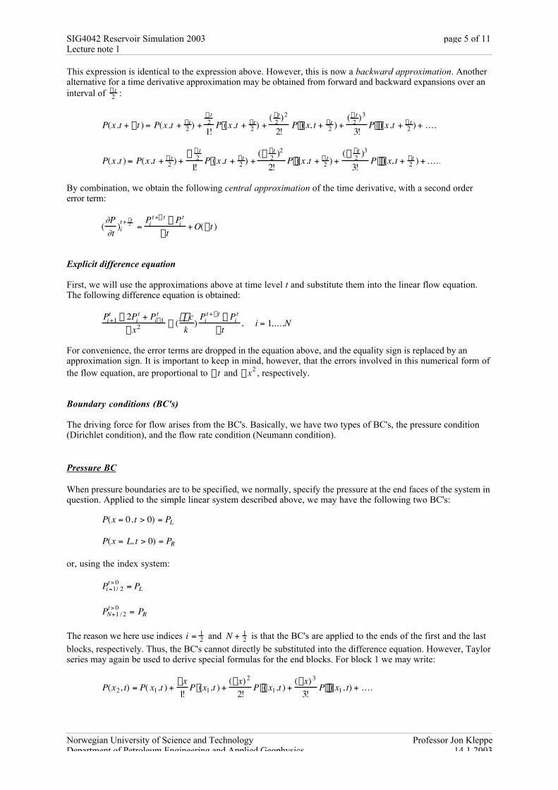
be subdivided into a number of discrete grid blocks, and the time coordinate must be divided into discrete timesteps. Then, the pressure in each block can be solved for numerically for each time step. For our simple onedimensional, horizontal porous slab, we thus define the following grid block system with N grid blocks, eachof length xD :This is called a block-centered grid, and the grid blocks are assigned indices, i , referring to the mid-point of

each block, representing the average property of the block.

Taylor series approximations

A so-called Taylor series approximation of a function f ( x + h) expressed in terms of f ( x)and its derivatives¢ f ( x) may be written:

f ( x + h) = f (x) +h1!

¢ f (x) +h2

2!¢ ¢ f (x) +

h3

3!¢ ¢ ¢ f (x) + .....

Applying Taylor series to our pressure function, we may write expansions in a variety of ways in order to obtainapproximations to the derivatives in the linear flow equation.

Approximation of the second order space derivative

At constant time, t, the pressure function may be expanded forward and backwards:

P(x + Dx, t) = P(x, t) +Dx1!

¢ P ( x, t) +(Dx)2

2!¢ ¢ P (x,t ) +

(Dx) 3

3!¢ ¢ ¢ P (x,t ) + .....

Dx

i-1 i i+1 N1



page 4 of 11

P(x - Dx, t) = P(x, t) +(- Dx)

1!¢ P (x,t ) +

(- Dx) 2

2!¢ ¢ P (x, t) +

(- Dx)3

3!¢ ¢ ¢ P (x, t) + .....

By adding these two expressions, and solving for the second derivative, we get the following approximation:

¢ ¢ P (x,t ) =P(x + Dx, t) - 2P(x,t ) + P(x + Dx,t )

(Dx)2 +(Dx) 2

12¢ ¢ ¢ ¢ P (x, t) + .....

or, by employing the grid index system, and using superscript to indicate time level:

(∂ 2P∂x 2 ) i

t =Pi +1

t - 2Pit + Pi -1

t

(Dx) 2 + O(Dx2 ) .

This is called a central approximation of the second derivative. Here, the rest of the terms from the Taylorseries expansion are collectively denoted O(Dx2 ) , thus denoting that they are in order of, or proportional in size

to 2xD . This error term, sometimes called discretization error, which in this case is of second order, isneglected in the numerical solution. The smaller the grid blocks used, the smaller will be the error involved.Any time level could be used in the expansions above. Thus, we may for instance write the followingapproximations at time levels t + Dt and t + D t

2 :

(∂ 2P∂x 2 ) i

t + Dt =Pi +1

t + Dt - 2Pit + Dt + Pi -1

t + Dt

(Dx)2 + O(Dx2 )

(∂2P

∂x2) i

t + D t2 =

Pi+1

t + Dt2 - 2Pi

t + Dt2 + Pi-1

t + Dt2

(Dx)2+ O(Dx2 )

Approximation of the time derivative

At constant position, x, the pressure function may be expanded in forward direction in regard to time:

P(x, t + Dt ) = P(x, t) +

Dt1!

¢ P (x, t ) +(Dt )2

2!¢ ¢ P (x, t ) +

(Dt )3

3!¢ ¢ ¢ P (x, t ) + .....

By solving for the first derivative, we get the following approximation:

¢ P (x,t ) =P(x,t + Dt ) - P(x, t)

Dt+

(Dt )2

¢ ¢ P (x,t ) + .....

or, employing the index system:

(∂P∂t

)it =

Pit + Dt - Pi

t

Dt+ O(Dt) .

Here, the error term is proportional to Dt , or of the first order. The error therefore approaches zero slower in thiscase than for the second order term above. This approximation is called a forward approximation. By expandingbackwards in time, we may write:

P(x,t ) = P(x,t + Dt ) +- Dt1!

¢ P (x, t + Dt) +(- Dt)2

2!¢ ¢ P (x, t + Dt) +

(- Dt)3

3!¢ ¢ ¢ P (x,t + Dt) + .....

Solving for the time derivative, we get:

(∂P∂t

)it + Dt =

Pit + Dt - Pi

t

Dt+ O(Dt) .



page 5 of 11

This expression is identical to the expression above. However, this is now a backward approximation. Anotheralternative for a time derivative approximation may be obtained from forward and backward expansions over aninterval of D t

2 :

P(x,t + Dt ) = P(x,t + Dt2 ) +

D t21!

¢ P (x,t + Dt2 ) +

( Dt2 )2

2!¢ ¢ P (x, t + Dt

2 ) +(D t

2 )3

3!¢ ¢ ¢ P (x,t + D t

2 ) + .....

P(x,t ) = P(x,t + D t2 ) +

- D t2

1!¢ P (x,t + Dt

2 ) +(- Dt

2 )2

2!¢ ¢ P (x,t + D t

2 ) +(- Dt

2 )3

3!¢ ¢ ¢ P (x, t + Dt

2 ) + .....

By combination, we obtain the following central approximation of the time derivative, with a second ordererror term:

(∂P∂t

)it + Dt

2 =Pi

t +D t - Pit

Dt+ O(Dt )

Explicit difference equation

First, we will use the approximations above at time level t and substitute them into the linear flow equation.The following difference equation is obtained:

Pi +1t - 2Pi

t + Pi-1t

Dx2 ª (fmck

)Pi

t + Dt - Pit

Dt, i = 1,...,N

For convenience, the error terms are dropped in the equation above, and the equality sign is replaced by anapproximation sign. It is important to keep in mind, however, that the errors involved in this numerical form ofthe flow equation, are proportional to Dt and Dx2 , respectively.

Boundary conditions (BC's)

The driving force for flow arises from the BC's. Basically, we have two types of BC's, the pressure condition(Dirichlet condition), and the flow rate condition (Neumann condition).

Pressure BC

When pressure boundaries are to be specified, we normally, specify the pressure at the end faces of the system inquestion. Applied to the simple linear system described above, we may have the following two BC's:

P(x = 0, t > 0) = PL

P(x = L, t > 0) = PR

or, using the index system:

Pi =1/ 2t > 0 = PL

PN+1 / 2t > 0 = PR

The reason we here use indices i = 12 and N + 1

2 is that the BC's are applied to the ends of the first and the lastblocks, respectively. Thus, the BC's cannot directly be substituted into the difference equation. However, Taylorseries may again be used to derive special formulas for the end blocks. For block 1 we may write:

P(x2, t) = P( x1,t ) +Dx1!

¢ P (x1,t ) +(Dx) 2

2!¢ ¢ P ( x1,t ) +

(Dx) 3

3!¢ ¢ ¢ P (x1, t) + .....



page 6 of 11

P(x = 0, t) = P(x1,t ) +(- Dx

2 )1!

¢ P (x1,t ) +(- Dx

2 )2

2!¢ ¢ P ( x1,t ) +

(- Dx2 )3

3!¢ ¢ ¢ P (x1, t) + .....

By combination of the two expressions, we obtain the following approximation of the second derivative inblock 1:

(∂ 2P∂x 2 )1

t =P2

t - 3P1t + 2PL

34 (Dx) 2 + O(Dx)

A disadvantage of this formulation is that the error term is only first order, i.e. proportional to Dx . A similarexpression may be obtained for the right hand side:

(∂ 2P∂x 2 ) N

t =2PR - 3PN

t + PN -1t

34 (Dx)2 + O(Dx) .

In a real reservoir case, pressure boundary conditions would normally represent bottom hole, or well head,pressures in production or injection wells.

Flow rate BC

Alternatively, we would specify the flow rate, Q , into or out of an end face of the system in question, forinstance into the left end of the system above. Making use of the fact that the flow rate may be expressed byDarcy's law, as follows:

QL = -k Am

∂P∂x

Ê Ë Á

ˆ ¯ ˜

x = 0.

We will again apply Taylor series expansion to block 1, but this time we will let the derivative of the pressurebe the function:

¢ P (x1 + Dx2 ,t ) = ¢ P (x1, t) +

( Dx2 )1!

¢ ¢ P (x1, t) +(Dx

2 )2

2!¢ ¢ ¢ P (x1,t ) + .....

¢ P (x = 0, t) = ¢ P (x1,t ) +(- Dx

2 )1!

¢ ¢ P (x1,t ) +(- Dx

2 )2

2!¢ ¢ ¢ P ( x1,t ) + .....

Subtracting the second expression from the first and solving for the second derivative, we obtain the followingapproximation for grid block 1:

¢ ¢ P (x1, t) =¢ P (x1 + Dx

2 , t) - ¢ P (x = 0, t)Dx

+ O(Dx2 )

Now we replace the derivative at the end face by the expression given by the boundary condition:

¢ ¢ P (x1, t) =¢ P (x1 + Dx

2 , t) + QLmk A

Dx+ O(Dx2 )

The other in the expression derivative may be replaced by a central formula:

¢ P (x1 + Dx2 ,t ) =

P(x2 ,t ) - P(x1, t)Dx

+ O(Dx2 ) ,

so that the final formula for the second derivative in block 1 for this boundary condition becomes:

(∂ 2P∂x 2 )1

t =P2

t - P1t

(Dx)2 + QLm

DxAk+ O(Dx)



page 7 of 11

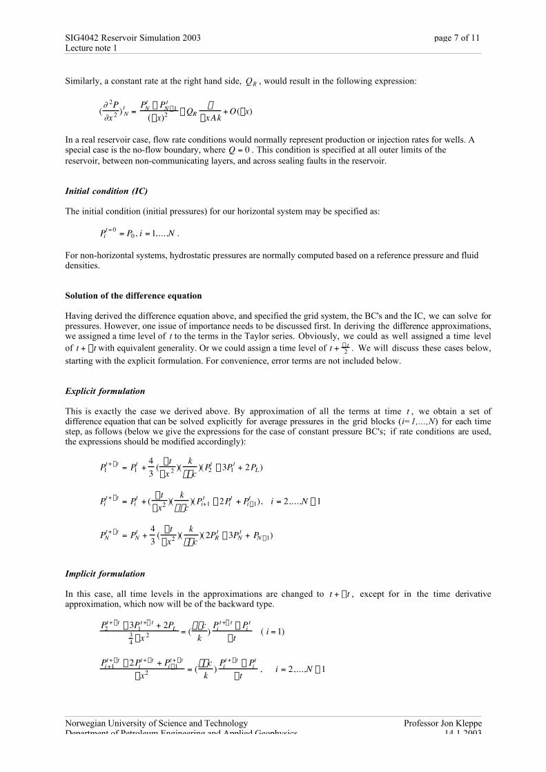
Similarly, a constant rate at the right hand side, RQ , would result in the following expression:

(∂ 2P∂x 2 ) N

t =PN

t - PN -1t

(Dx)2 - QRm

DxAk+ O(Dx)

In a real reservoir case, flow rate conditions would normally represent production or injection rates for wells. Aspecial case is the no-flow boundary, where Q = 0 . This condition is specified at all outer limits of thereservoir, between non-communicating layers, and across sealing faults in the reservoir.

Initial condition (IC)

The initial condition (initial pressures) for our horizontal system may be specified as:

Pit = 0 = P0, i = 1,...,N .

For non-horizontal systems, hydrostatic pressures are normally computed based on a reference pressure and fluiddensities.

Solution of the difference equation

Having derived the difference equation above, and specified the grid system, the BC's and the IC, we can solve forpressures. However, one issue of importance needs to be discussed first. In deriving the difference approximations,we assigned a time level of t to the terms in the Taylor series. Obviously, we could as well assigned a time levelof t + Dt with equivalent generality. Or we could assign a time level of t + D t

2 . We will discuss these cases below,starting with the explicit formulation. For convenience, error terms are not included below.

Explicit formulation

This is exactly the case we derived above. By approximation of all the terms at time t , we obtain a set ofdifference equation that can be solved explicitly for average pressures in the grid blocks (i=1,...,N) for each timestep, as follows (below we give the expressions for the case of constant pressure BC's; if rate conditions are used,the expressions should be modified accordingly):

P1t + Dt = P1

t +43

(Dt

Dx 2 )(k

fmc)(P2

t - 3P1t + 2PL )

Pit + Dt = Pi

t + (Dt

Dx2 )(k

fmc)(Pi+1

t - 2Pit + Pi -1

t ), i = 2,...,N - 1

PNt + Dt = PN

t +43

(Dt

Dx2 )(k

fmc)(2PR

t - 3PNt + PN -1)

Implicit formulation

In this case, all time levels in the approximations are changed to t + Dt , except for in the time derivativeapproximation, which now will be of the backward type.

P2t + Dt - 3P1

t +D t + 2PL34 Dx 2 = (

fmck

)Pi

t +D t - Pit

Dt( i = 1)

Pi +1t + Dt - 2Pi

t + Dt + Pi -1t + Dt

Dx2 = (fmc

k)

Pit + Dt - Pi

t

Dt, i = 2,...,N - 1



page 8 of 11

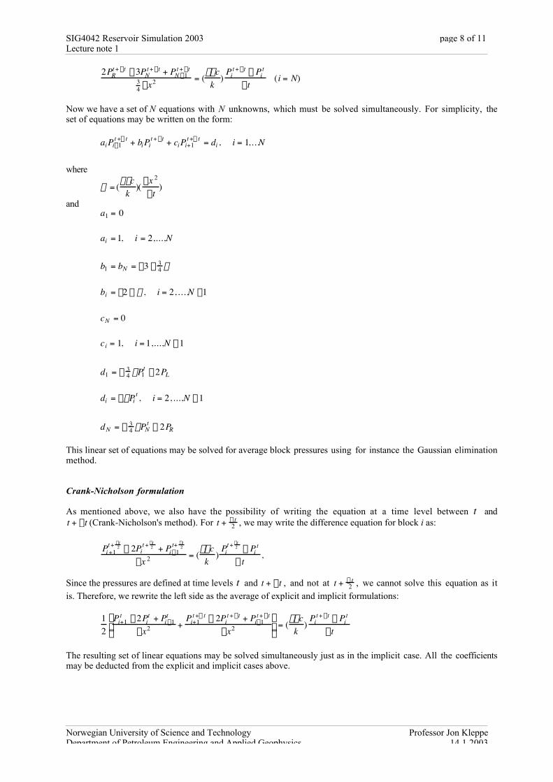
2PRt + Dt - 3PN

t + Dt + PN -1t + Dt

34 Dx2 = (

fmck

)Pi

t + Dt - Pit

Dt(i = N)

Now we have a set of N equations with N unknowns, which must be solved simultaneously. For simplicity, theset of equations may be written on the form:

aiPi-1t +D t + biPi

t + Dt + ciPi+1t +D t = di , i = 1,...N

where

a = (fmc

k)(

Dx 2

Dt)

anda1 = 0

ai = 1, i = 2,...,N

b1 = bN = -3 - 34 a

bi = -2 - a , i = 2, ...,N -1

cN = 0

ci = 1, i = 1,...,N - 1

d1 = - 34 aP1

t - 2PL

di = -aPit , i = 2, ...,N - 1

dN = - 34 aPN

t - 2PR

This linear set of equations may be solved for average block pressures using for instance the Gaussian eliminationmethod.

Crank-Nicholson formulation

As mentioned above, we also have the possibility of writing the equation at a time level between t andt + Dt (Crank-Nicholson's method). For t + D t

2 , we may write the difference equation for block i as:

Pi +1t + Dt

2 - 2Pit + Dt

2 + Pi -1t+ Dt

2

Dx 2 = (fmck

)Pi

t + Dt2 - Pi

t

Dt,

Since the pressures are defined at time levels t and t + Dt , and not at t + D t2 , we cannot solve this equation as it

is. Therefore, we rewrite the left side as the average of explicit and implicit formulations:

12

Pi+1t - 2Pi

t + Pi -1t

Dx2 +Pi+1

t +D t - 2Pit + Dt + Pi-1

t + Dt

Dx2È

Î Í

˘

˚ ˙ = (

fmck

)Pi

t + Dt - Pit

Dt

The resulting set of linear equations may be solved simultaneously just as in the implicit case. All the coefficientsmay be deducted from the explicit and implicit cases above.



page 9 of 11

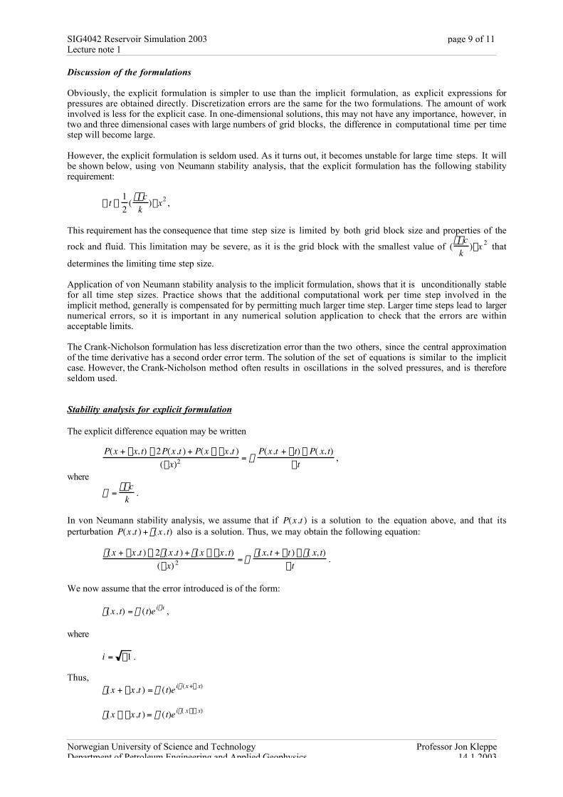
Discussion of the formulations

Obviously, the explicit formulation is simpler to use than the implicit formulation, as explicit expressions forpressures are obtained directly. Discretization errors are the same for the two formulations. The amount of workinvolved is less for the explicit case. In one-dimensional solutions, this may not have any importance, however, intwo and three dimensional cases with large numbers of grid blocks, the difference in computational time per timestep will become large.

However, the explicit formulation is seldom used. As it turns out, it becomes unstable for large time steps. It willbe shown below, using von Neumann stability analysis, that the explicit formulation has the following stabilityrequirement:

Dt £12

(fmck

)Dx2 ,

This requirement has the consequence that time step size is limited by both grid block size and properties of the

rock and fluid. This limitation may be severe, as it is the grid block with the smallest value of (fmc

k)Dx 2 that

determines the limiting time step size.

Application of von Neumann stability analysis to the implicit formulation, shows that it is unconditionally stablefor all time step sizes. Practice shows that the additional computational work per time step involved in theimplicit method, generally is compensated for by permitting much larger time step. Larger time steps lead to largernumerical errors, so it is important in any numerical solution application to check that the errors are withinacceptable limits.

The Crank-Nicholson formulation has less discretization error than the two others, since the central approximationof the time derivative has a second order error term. The solution of the set of equations is similar to the implicitcase. However, the Crank-Nicholson method often results in oscillations in the solved pressures, and is thereforeseldom used.

Stability analysis for explicit formulation

The explicit difference equation may be written

P(x + Dx, t) - 2P(x,t ) + P(x - Dx,t )(Dx)2 = a

P(x,t + Dt) - P( x, t)Dt

,

where

a =fmc

k.

In von Neumann stability analysis, we assume that if P(x,t ) is a solution to the equation above, and that itsperturbation P(x,t ) + e(x, t) also is a solution. Thus, we may obtain the following equation:

e(x + Dx,t ) - 2e(x,t ) + e(x - Dx, t)(Dx) 2 = a

e(x, t + Dt ) - e( x, t)Dt

.

We now assume that the error introduced is of the form:

e(x, t) = y (t)eibx ,

where

i = -1 .

Thus,e(x + Dx,t ) = y (t)eib (x +D x)

e(x - Dx,t ) = y (t)eib( x -D x)



page 10 of 11

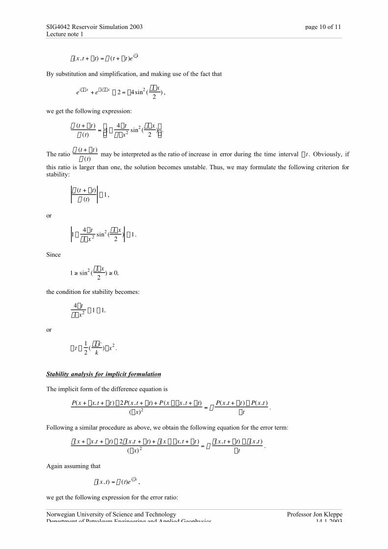
e(x, t + Dt) = y (t + Dt )eibx

By substitution and simplification, and making use of the fact that

eibDx + e-ibDx - 2 = -4sin2 (bDx2

) ,

we get the following expression:

y (t + Dt )y (t)

= 1-4Dt

aDx2 sin2 (bDx

2)È

Î Í ˘ ˚ ˙ .

The ratio y (t + Dt )

y (t) may be interpreted as the ratio of increase in error during the time interval Dt . Obviously, if

this ratio is larger than one, the solution becomes unstable. Thus, we may formulate the following criterion forstability:

y (t + Dt)y (t)

£ 1 ,

or

1-4Dt

aDx 2 sin2 (bDx

2) £ 1.

Since

1 ≥ sin2 (bDx

2) ≥ 0,

the condition for stability becomes:

4DtaDx2 - 1 £ 1,

or

Dt £12

(fmck

)Dx2 .

Stability analysis for implicit formulation

The implicit form of the difference equation is

P(x + Dx, t + Dt ) - 2P(x, t + Dt) + P(x - Dx, t + Dt)(Dx)2 = a

P(x,t + Dt ) - P(x,t )Dt

.

Following a similar procedure as above, we obtain the following equation for the error term:

e(x + Dx,t + Dt) - 2e(x,t + Dt) + e(x - Dx, t + Dt )(Dx) 2 = a

e(x, t + Dt) - e(x,t )Dt

.

Again assuming that

e(x, t) = y (t)eibx ,

we get the following expression for the error ratio:



page 11 of 11

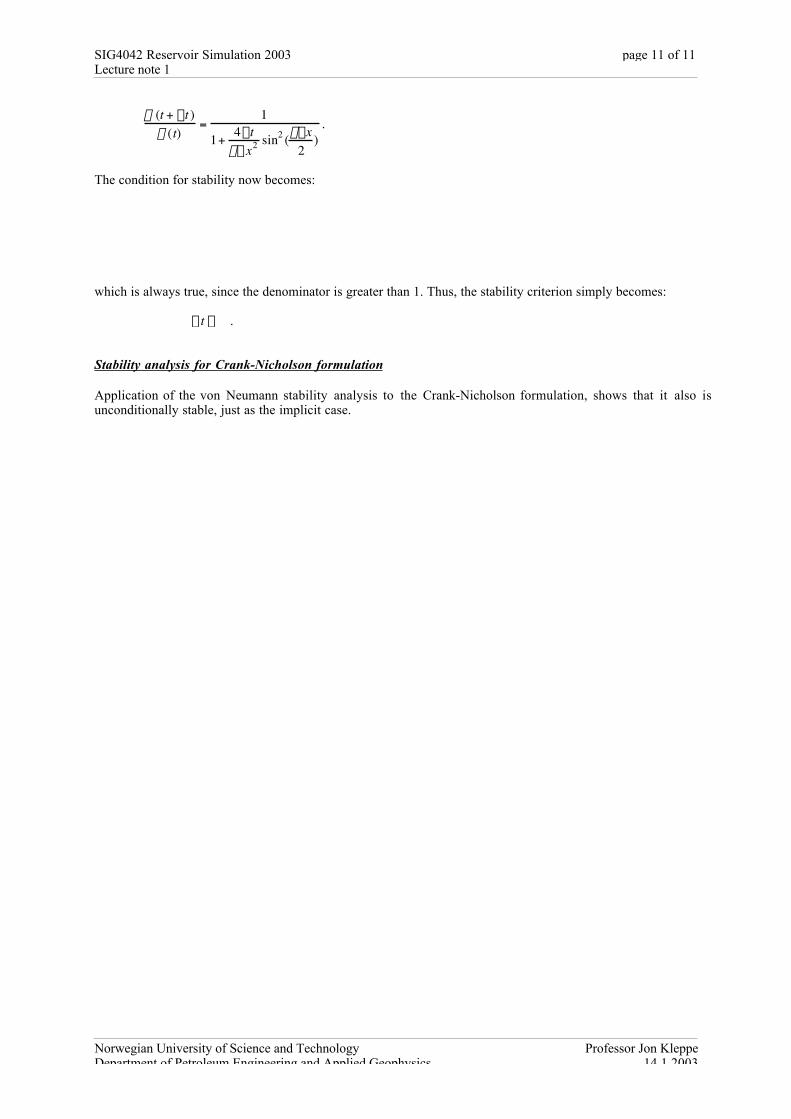
y (t + Dt )y (t)

=1

1+4Dt

aDx2 sin2 (bDx2

).

The condition for stability now becomes:

which is always true, since the denominator is greater than 1. Thus, the stability criterion simply becomes:

Dt £ • .

Stability analysis for Crank-Nicholson formulation

Application of the von Neumann stability analysis to the Crank-Nicholson formulation, shows that it also isunconditionally stable, just as the implicit case.

Documents

Reservoir simulation_Note01