Resetting Virtual Absorbers for Vibration Control Virtual Absorbers for Vibration Control ROBERT T. BUPP TRW S & EG Redondo Beach, CA 90278, USA DENNIS S. BERNSTEIN Department of Aerospace

Resetting Virtual Absorbers for Vibration Control

ROBERT T. BUPPTRW S & EG Redondo Beach, CA 90278, USA

DENNIS S. BERNSTEINDepartment of Aerospace Engineering The University of Michigan Ann Arbor, MI 48109-2140,USA

VIJAYA S. CHELLABOINAWASSIM M. HADDADSchool of Aerospace Engineering Georgia Institute of Technology Atlanta, GA 30332-0150, USA

(Received 8 November 1996; accepted 21 April 1998)

Abstract: A novel class of controllers, called resetting virtual absorbers, is proposed as a means for achievingenergy dissipation. A general framework for analyzing resetting virtual absorbers is given, and stability ofthe closed-loop system is analyzed. Special cases of resetting virtual absorbers, called the virtual trap-doorabsorber and the virtual one-way absorber, are described, and some illustrative examples are given.

Key Words: Resetting controllers, virtual absorbers, impulsive differential equations

1. INTRODUCTION

For more than 100 years, many different types of vibration absorbers have been used toremove energy from mechanical systems or to block energy from entering a system (Frahm,1909; Watts, 1883). The design of dynamic vibration absorbers has received considerableattention since the mathematical description of the Den Hartog absorber (Den Hartog, 1956;Ormondroyd and Den Hartog, 1928; Snowdon, 1968), and their use is widespread today(Korenov and Reznikov, 1993).

Dynamic vibration absorbers are passive devices that have the appealing quality that,once properly designed, built, and installed, will generally operate without further attentionor energy input. However, for additional flexibility, virtual absorbers have recently beenintroduced (Phan et al., 1993; Juang and Phan, 1992). A virtual absorber emulates theeffect of a physical absorber by sensing the motion of the primary structure, utilizing adynamic compensator to simulate the motion that a physical absorber would undergo, andcomputing and applying the reaction force that the physical absorber would apply to theprimary structure. The computed reaction force is then implemented by means of a suitableactuator. Thus, the implementation of a virtual absorber requires the availability of sensorsand actuators as well as processors and power supplies. One advantage of virtual absorbers

Journal of Vibration and Control, �� 61-83, 2000f?2000 Sage Publications, Inc.

62 R. T. BUPP ET AL.

over passive absorbers is that the parameters of the virtual absorber can be adjusted online(Lai and Wang, 1996; Sun, Jolly, and Norris, 1995; Quan and Stech, 1996).

An important feature of physical absorbers is that their components can be associatedwithsome form of energy, usually kinetic or potential. In a mechanical system, positions typicallycorrespond to elastic deformations, which contribute to the potential energy of the system,whereas velocities typically correspond to momenta, which contribute to the kinetic energy ofthe system. On the other hand, while a virtual absorber has dynamic states that emulate themotion of the physical components, these states only òòexistóó as numerical representationsinside the processor. Consequently, while one can associate an emulated energy with thesestates, this energy is merely a mathematical construct and does not correspond to any physicalform of energy.

In vibration control problems, if a plant is at a high energy level, and a physical absorberat a low energy level is attached to it, then energy will generally tend to flow from the plantinto the absorber, decreasing the plant energy and increasing the absorber energy (Kishimoto,Bernstein, and Hall, 1995). Conversely, if the plant is at a low energy level and an attachedabsorber is at a high energy level, then energy will tend to flow from the absorber into theplant. This behavior is also exhibited by a plant with an attached virtual absorber, althoughin this case, emulated energy, and not physical energy, is accumulated by the virtual absorber.Nonetheless, energy can flow from a virtual absorber to the plant, since a virtual absorberwith emulated energy can generate real, physical energy to effect the required energy flow.Therefore, when using a virtual absorber, it may be advantageous to detect when the positionand velocity states of the emulated absorber represent a high emulated energy level, and thenreset these states to remove the emulated energy so that the emulated energy is not returned tothe plant. A virtual absorber whose states are reset is called a resetting virtual absorber. Thecontribution of this paper is the development of resetting virtual absorbers as a novel strategyfor vibration suppression.

The concept of a resetting virtual absorber can be viewed as a specialized technique forexploiting the coupling between a structure and a passive controller to remove energy fromthe structure. This idea provides the motivation for synthesizing positive real controllersfor positive real plants using K5 and K4 methods (Bupp et al., 1995; Haddad, Bernstein,and Wang, 1994; Haddad and Chellaboina, 1997; Lozano-Leal and Joshi, 1988; Kishimoto,Bernstein, and Hall, 1995). In addition, in a series of papers (Duquette, Tuer, and Golnaraghi,1993; Golnaraghi, Tuer, and Wang, 1994, 1995; Tuer, Golnaraghi, and Wang, 1994; Ouceiniand Golnaraghi, 1996; Ouceini, Tuer, and Golnaraghi, 1995; Siddiqui and Golnaraghi,1996), M. F. Golnaraghi and coworkers have developed and demonstrated a modal couplingtechnique that utilizes energy transfer phenomena and a resetting mechanism to suppressstructural vibration. The present paper thus provides a systematic investigation of variousrealizations of this idea in terms of resetting differential equations.

This paper presents a review in Section 2 of the concept of resetting differential equations,which provide the mathematical foundation for analyzing resetting virtual absorbers. Twokinds of resetting virtual absorbers, namely, time-dependent and state-dependent resettingvirtual absorbers, are then described in Section 3, and illustrative examples are provided.Conclusions are presented in Section 4.

RESETTING VIRTUAL ABSORBERS 63

2. MATHEMATICAL PRELIMINARIES

In this section, we review some basic results on resetting differential equations (Bainov andSimeonov, 1989; Kulev and Bainov, 1989; Lakshmikantham, Leela, and Martynyuk, 1989;Lakshmikantham, Leela, and Kaul, 1994; Lakshmikantham, Bainov, and Simeonov, 1989;Lakshmikantham and Liu, 1989; Liu, 1988; Simeonov and Bainov, 1985, 1987), which willbe used throughout the paper to analyze resetting virtual absorbers. A resetting differentialequation consists of three elements:

1. A continuous-time dynamical equation, which governs the motion of the system be-tween resetting events;

2. A difference equation, which governs the way the states are instantaneously changedwhen a resetting event occurs; and

3. A criterion for determining when the states of the system are to be reset.

A resetting differential equation thus has the form

b{+w , @ i +{+w ,,> +w> {+w ,, @5 V> (1)

�{+w , @ �+{+w ,,> +w> {+w ,, 5 V> (2)

where w � 3, {+w , 5 Uq , i = Uq $ Uq is Lipschitz continuous and satisfies i +3, @ 3;

� = Uq $ Uq and satisfies �+3, @ 3, and V � ^3>4, � Uq is the resetting set. We refer

to the differential equation (1) as the continuous-time dynamics, and we refer to the differenceequation (2) as the resetting law. For convenience, we use the notation {+w > � > � , to denotethe solution of (1) at time w A � with initial condition {+�, @ � .

For a particular trajectory {+w ,, we let wn denote the nth instant of time at which +w> {+w ,,intersects V, and we call the times wn the resetting times. Thus the trajectory of the system (1),(2) from the initial condition {+3, @ {3 is given by {+w > 3> {3, for 3 ? w � w4. If and when the

trajectory reaches a state {47@ {+w4, satisfying +w4> {4, 5 V, then the state is instantaneously

transferred to {.47@ {4 . �+{4, according to (2). The trajectory {+w ,, w4 ? w � w5, is then

given by {+w > w4> {.4 ,, and so on. Note that the solution {+w , of (1), (2) is left continuous; that

is, it is continuous everywhere except at the resetting times wn , and

{n7@ {+wn , @ olp

%$3.{+wn � %,> (3)

{.n7@ {+wn , . �+{+wn ,, @ olp

%$3.{+wn . %,> (4)

for n @ 4> 5> = = = =We make the following additional assumptions:

A1. +3> {3, @5 V, where {+3, @ {3, that is, the initial condition is not in V.


A2. If +w> {+w ,, 5 fo V q V, where cl V denotes the closure of the set V, then there exists% A 3 such that, for all 3 ? � ? %,

{+w. �> w> {+w ,, @5 V=

A3. If +w> {+w ,, 5 fo VWV, then there exists % A 3 such that, for all 3 ? � ? %,

{+w. �> w> {+w , . �+{+w ,,, @5 V=

Assumption A1 ensures that the initial condition for the resetting differential equation (1),(2) is not a point of discontinuity, and this assumption is made for convenience and withoutloss of generality. If +3> {3, 5 V, then the system initially resets to {.3 @ {3 . �+{3,, whichserves as the initial condition for the continuous-time dynamics (1). It follows from A3 thatthe trajectory then leaves V. We assume in A2 that if a trajectory reaches the closure of V ata point that does not belong to V, then the trajectory must be directed away from V, that is, atrajectory cannot enter V through a point that belongs to the closure of V but not to V. Finally,A3 ensures that when a trajectory intersects the resetting set V, it instantaneously exits V.

Remark 2.1. It follows from A3 that resetting removes the pair +wn > {n , from the resettingset V. Thus, immediately after resetting occurs, the continuous-time dynamics (1), and notthe resetting law (2), becomes the active element of the resetting differential equation.

Remark 2.2. It follows from A1ðA3 that no trajectory can intersect the interior of V:According to A1, the trajectory {+w , begins outside the set V. Furthermore, it follows fromA2 that a trajectory can only reach V at a point belonging to both V and its closure. Finally,from A3, it follows that if a trajectory reaches a point in V that is in the closure of V, then thetrajectory is instantaneously removed from V. Since a continuous trajectory starting outsideof V and intersecting the interior of V must first intersect the closure of V, it follows that notrajectory can reach the interior of V.

Remark 2.3. It follows from A1ðA3 and Remark 2.2 that the resetting times wn are welldefined and distinct.

Remark 2.4. Since the resetting times are well defined and distinct, and since solutions of(1) exist and are unique, it follows that the solutions of the resetting differential equation (1),(2) also exist and are unique in forward time.

In Bainov and Simeonov (1989); Hu, Lakshmikantham, and Leela (1989); Sun, Jolly, andNorris (1995); Lakshmikantham, Bainov, and Simeonov (1989); Lakshmikantham, Leela,and Kaul (1994); Lakshikantham and Liu (1989); Liu (1988); and Simeonov and Bainov(1985, 1987), the resetting set V is defined in terms of a countable number of functions� n = Uq $ +3>4, and is given by

V @^n

i+� n +{,> {, = { 5 Uq j = (5)


The analysis of resetting differential equations with a resetting set of the form (5) can be quiteinvolved. Here we consider resetting differential equations involving two distinct forms ofthe resetting set V. In the first case, the resetting set is defined by a prescribed sequenceof times that are independent of the state {. These equations are thus called time-dependentresetting differential equations. In the second case, the resetting set is defined by a region in thestate space that is independent of time. These equations are called state-dependent resettingdifferential equations.

2.1. Time-Dependent Resetting Differential Equations

Time-dependent resetting differential equations, which are studied in Simeonov and Bainov(1985) and Lakshmikantham, Bainov, and Simeonov (1989), can be written as (1), (2) withV defined as

V 7@ W � Uq > (6)

where

W 7@ iw4> w5> = = =j (7)

and 3 ? w4 ? w5 ? � � � are prescribed resetting times. When an infinite number of resettingtimes are used, we assume that wn $ 4 as n$ 4 so that V is closed. Now (1), (2) can berewritten in the form of the time-dependent resetting differential equation

b{+w , @ i +{+w ,,> w 9@ wn > (8)

�{+w , @ �+{+w ,,> w @ wn = (9)

Since 3 @5 W and wn ? wn.4 , it follows that the assumptions A1ðA3 are satisfied. For ourpurposes, the following stability result is needed. Note that the usual stability definitions arevalid.

Theorem 2.1. Suppose there exists a continuously differentiable function Y = Uq $ ^3>4,satisfying Y +3, @ 3, Y +{, A 3, { 9@ 3, and

Y 3+{, i +{, � 3> { 5 Uq > (10)

Y +{ . �+{,, � Y +{,> { 5 Uq = (11)

Then the zero solution of (8), (9) is Lyapunov stable. Furthermore, if the inequality in (10) is strictfor all { 9@ 3, then the zero solution of (8), (9) is asymptotically stable. If, in addition,

Y +{,$4 as mm{mm $ 4> (12)


then the zero solution of (8), (9) is globally asymptotically stable.

Proof. Prior to the first resetting time, we can determine the value of Y +{+w ,, as

Y +{+w ,, @ Y +{+3,, .

] w

3

Y 3+{+�,, i +{+�,,g� > w 5 ^3> w4`= (13)

Between consecutive resetting times wn and wn.4 , we can determine the value of Y +{+w ,, asits initial value plus the integral of its rate of change along the trajectory {+w ,, that is,

Y +{+w ,, @ Y +{n . �+{n ,, .

] w

wn

Y 3+{+�,, i +{+�,,g� > w 5 +wn > wn.4 `> (14)

for n @ 4> 5> = = = = Adding and subtracting Y +{n , to the right-hand side of (14) yields

Y +{+w ,, @ Y +{n , . ^Y +{n . �+{n ,,� Y +{n ,`

.

] w

wn

Y 3+{+�,, i +{+�,,g� > w 5 +wn > wn.4 `> (15)

and in particular at time wn.4 ,

Y +{n.4 , @ Y +{n , . ^Y +{n . �+{n ,,� Y +{n ,` .

] wn .4

wn

Y 3+{+�,, i +{+�,,g� = (16)

By recursively substituting (16) into (15) and ultimately into (13), we obtain

Y +{+w ,, @ Y +{+3,, .

] w

3

Y 3+{+�,, i +{+�,,g�

.n[

l@4

^Y +{+wl , . �+{+wl ,,,� Y +{+wl ,,` > w 5 +wn > wn.4 `= (17)

If we allow w37@ 3, and

S3

l@4

7@ 3, then (17) is valid for n @ 3> 4> 5> = = = = From (17) and

(11), we obtain

Y +{+w ,, � Y +{+3,, .

] w

3

Y 3+{+�,, i +{+�,,g� > w � 3= (18)

Furthermore, it follows from (10) that

Y +{+w ,, � Y +{+3,,> w � 3> (19)

so that Lyapunov stability follows from standard arguments.


Next, it follows from (11) and (17) that

Y +{+w ,,� Y +{+v,, �] w

v

Y 3+{+�,, i +{+�,,g� > w A v> (20)

and, assuming strict inequality in (10), we obtain

Y +{+w ,, ? Y +{+v,,> w A v> (21)

provided {+v, 9@ 3. Asymptotic stability, and with (12) global asymptotic stability, thenfollow from standard arguments.

Remark 2.5. In the proof of Theorem 2.1, we note that assuming strict inequality in (10),the inequality (21) is obtained provided {+v, 9@ 3. This proviso is necessary since it may bepossible to reset the states to the origin, in which case {+v, @ 3 for a finite value of v. Inthis case, for w A v, we have Y +{+w ,, @ Y +{+v,, @ Y +3, @ 3. This situation does notpresent a problem, however, since reaching the origin in finite time is a stronger conditionthan reaching the origin as w$4.

2.2. State-Dependent Resetting Differential Equations

State-dependent resetting differential equations, which are discussed in Bainov and Simeonov(1989), can be written as (1), (2) with V defined as

V 7@ ^3>4,�P> (22)

where P � Uq . Therefore, (1), (2) can be rewritten in the form of the state-dependent

resetting differential equation

b{+w , @ i +{+w ,,> {+w , @5P> (23)

�{+w , @ �+{+w ,,> {+w , 5P= (24)

We assume that {3 @5 P, 3 @5 P, and that the resetting action removes the state from thesetP; that is, if { 5 P, then { . �+{, @5 P. In addition, we assume that if at time w thetrajectory {+w , 5 foPqP, then there exists % A 3 such that for 3 ? � ? %, {+w.�, @5P.These assumptions represent the specializations of A1ðA3 for the particular resetting set (22).It follows from these assumptions that for a particular initial condition, the resetting times wnare distinct and well defined.

Remark 2.6. Let {� 5 Uq satisfy �+{�, @ 3. Then {� @5P. To see this, suppose {� 5P.Then {� . �+{�, @ {� 5 P, which contradicts the assumption that if { 5 P, then{ . �+{, @5P.

For our purposes, the following result for the stability of the zero solution is needed.


Theorem 2.2. Suppose there exists a continuously differentiable function Y = Uq $ ^3>4,satisfying Y +3, @ 3, Y +{, A 3, { 9@ 3, and

Y 3+{, i +{, � 3> { @5P> (25)

Y +{ . �+{,, � Y +{,> { 5P= (26)

Then the zero solution of (23), (24) is Lyapunov stable. Furthermore, if the inequality in (25) isstrict for all { 9@ 3, then the zero solution of (23), (24) is asymptotically stable. If, in addition,(12) is satisfied, then the zero solution of (23), (24) is globally asymptotically stable.

Because the resetting times are well defined and distinct for any trajectory of (23), (24),the proof of Theorem 2.2 follows from the proof of Theorem 2.1 given in Subsection 2.1.

3. RESETTING VIRTUAL ABSORBERS

In this section, we apply the theory of resetting differential equations to the analysis ofresetting virtual absorbers. We consider a continuous-time plant of the form

b{s+w , @ i s+{s+w ,> x+w ,,> (27)

|+w , @ ks+{s+w ,,> (28)

where {s 5 Uqf , i s = Uqs � U

p $ Uqs is continuously differentiable and satisfies

i s+3> 3, @ 3, and ks = Uqs $ Us is continuous and satisfies ks+3, @ 3. We also consider a

controller of the form

b{f+w , @ i f+{f+w ,> |+w ,,> +w> {f+w ,> |+w ,, @5 Vf > (29)

�{f+w , @ �f+{f+w ,> |+w ,,> +w> {f+w ,> |+w ,, 5 Vf > (30)

x+w , @ kf+{f+w ,> |+w ,,> (31)

where Vf � ^3>4, � Uqf � U

s , {f 5 Uqf , i f = Uqf � U

s $ Uqf is continuously

differentiable and satisfies i f+3> 3, @ 3, kf = Uqf � Us $ U

p is continuous andsatisfies kf+3> 3, @ 3, and � = Uqf � U

s $ Uqf satisfies �f+3> 3, @ 3. We assume

{f+3, @ �f+3> ks+{s+3,,,, which is generally a nonzero initial condition for the controller.The equations of motion for the closed-loop system (27) through (31) have the form


b{+w , @ i +{+w ,,> +w> {+w ,, @5 V> (32)

�{+w , @ �+{+w ,,> +w> {+w ,, 5 V> (33)

where

i +{,7@

�i s+{s > kf+{f> ks+{s,,,

i f+{f> ks+{s,,

�> {

7@

�{s

{f

�5 U

qs .qf > (34)

�+{,7@

�3

�f+{f > ks+{s,,

�(35)

and

V 7@ i+w> {, = +w> {f> ks+{s,, 5 Vfj = (36)

Note that q7@ qs . qf in the notation of Section 2.

Notice that (32), (33) has the form of the resetting differential equation (1), (2). However,while the closed-loop state vector consists of plant states and controller states, it is clear from(35) that only those states associated with the controller are reset.

We associate with the plant a positive-definite, continuously differentiable functionYs+{s,, satisfyingYs+3, @ 3>whichwewill refer to as the plant energy. We associate with thecontroller a nonnegative-definite, continuously differentiable function Yf+{f > |,, satisfyingYf+3> 3, @ 3 and Yf+{f > 3, A 3> {f 9@ 3, called the emulated energy. Finally, we associatewith the closed-loop system the function

Y+{,7@ Ys+{s, . Yf+{f > |,> (37)

called the total energy.

3.1. Time-Dependent Resetting Virtual Absorber

Consider the closed-loop system (32), (33) with resetting set defined by (6), (7) and wherethe prescribed elements of W satisfy 3 ? w4 ? w5 ? � � �. Suppose that Yf satisfies

Yf+{f . �f+{s > ks+{s,,, � Yf+{f > ks+{s,,> (38)

and Y +{, defined in (37) satisfies

Y 3+{, i +{, � 3> { 5 Uq = (39)

Then Lyapunov (resp., asymptotic) stability of the closed-loop system follows from Theorem2.1. The design of time-dependent resetting virtual absorbers is considered in the followingexamples.


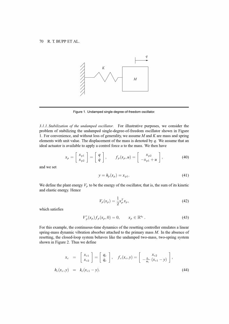
)LJXUH �� 8QGDPSHG VLQJOH�GHJUHH�RI�IUHHGRP RVFLOODWRU�

3.1.1. Stabilization of the undamped oscillator. For illustrative purposes, we consider theproblem of stabilizing the undamped single-degree-of-freedom oscillator shown in Figure1. For convenience, and without loss of generality, we assumeP and N are mass and springelements with unit value. The displacement of the mass is denoted by t. We assume that anideal actuator is available to apply a control force x to the mass. We then have

{s @

�{s4{s5

�@

�tbt

�> i s+{s > x, @

�{s5

�{s4 . x

�> (40)

and we set

| @ ks+{s, @ {s4= (41)

We define the plant energy Ys to be the energy of the oscillator, that is, the sum of its kineticand elastic energy. Hence

Ys+{s, @4

5{Ws {s > (42)

which satisfies

Y 3s+{s, i s+{s > 3, @ 3> {s 5 Uqs = (43)

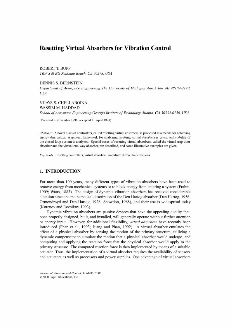
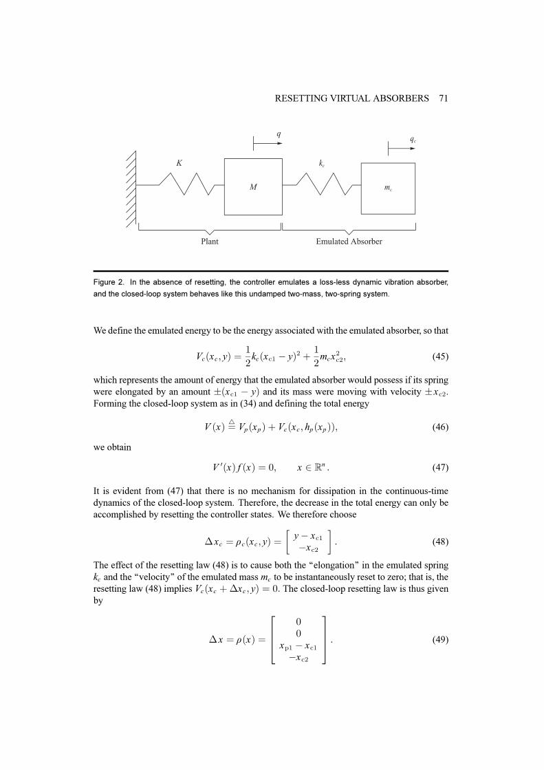
For this example, the continuous-time dynamics of the resetting controller emulates a linearspring-mass dynamic vibration absorber attached to the primary mass P. In the absence ofresetting, the closed-loop system behaves like the undamped two-mass, two-spring systemshown in Figure 2. Thus we define

{f @

�{f4{f5

�@

�tfbtf

�> i f+{f> |, @

�{f5

� nfpf

+{f4 � |,

�>

kf+{f > |, @ nf+{f4 � |,= (44)


)LJXUH �� ,Q WKH DEVHQFH RI UHVHWWLQJ� WKH FRQWUROOHU HPXODWHV D ORVV�OHVV G\QDPLF YLEUDWLRQ DEVRUEHU�

DQG WKH FORVHG�ORRS V\VWHP EHKDYHV OLNH WKLV XQGDPSHG WZR�PDVV� WZR�VSULQJ V\VWHP�

We define the emulated energy to be the energy associated with the emulated absorber, so that

Yf+{f> |, @4

5nf+{f4 � |,5 .

4

5pf{

5f5> (45)

which represents the amount of energy that the emulated absorber would possess if its springwere elongated by an amount +{f4 � |, and its mass were moving with velocity {f5.Forming the closed-loop system as in (34) and defining the total energy

Y +{,7@ Ys+{s, . Yf+{f > ks+{s,,> (46)

we obtain

Y 3+{, i +{, @ 3> { 5 Uq = (47)

It is evident from (47) that there is no mechanism for dissipation in the continuous-timedynamics of the closed-loop system. Therefore, the decrease in the total energy can only beaccomplished by resetting the controller states. We therefore choose

�{f @ �f+{f > |, @

�|� {f4�{f5

�= (48)

The effect of the resetting law (48) is to cause both the òòelongationóó in the emulated springnf and the òòvelocityóó of the emulated mass pf to be instantaneously reset to zero; that is, theresetting law (48) implies Yf+{f .�{f > |, @ 3= The closed-loop resetting law is thus givenby

�{ @ �+{, @

5997

33

{s4 � {f4�{f5

6::8 = (49)


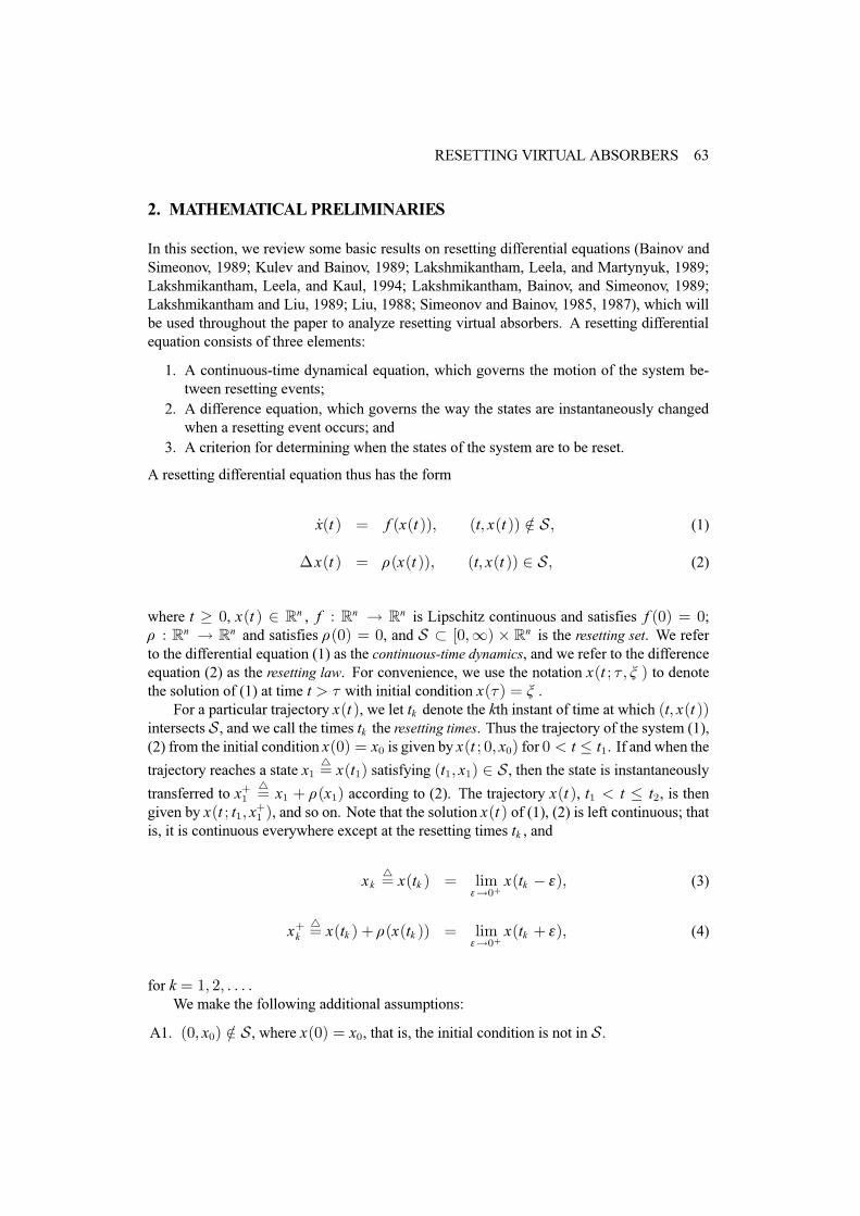
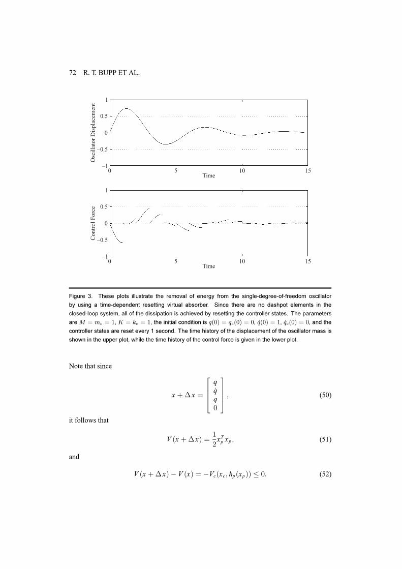
)LJXUH �� 7KHVH SORWV LOOXVWUDWH WKH UHPRYDO RI HQHUJ\ IURP WKH VLQJOH�GHJUHH�RI�IUHHGRP RVFLOODWRU

E\ XVLQJ D WLPH�GHSHQGHQW UHVHWWLQJ YLUWXDO DEVRUEHU� 6LQFH WKHUH DUH QR GDVKSRW HOHPHQWV LQ WKH

FORVHG�ORRS V\VWHP� DOO RI WKH GLVVLSDWLRQ LV DFKLHYHG E\ UHVHWWLQJ WKH FRQWUROOHU VWDWHV� 7KH SDUDPHWHUV

DUH � ' 6S ' �� g ' &S ' �� WKH LQLWLDO FRQGLWLRQ LV Êf� ' ^SEf� ' f� �̂Ef� ' �� ̂SEf� ' f� DQG WKH

FRQWUROOHU VWDWHV DUH UHVHW HYHU\ � VHFRQG� 7KH WLPH KLVWRU\ RI WKH GLVSODFHPHQW RI WKH RVFLOODWRU PDVV LV

VKRZQ LQ WKH XSSHU SORW� ZKLOH WKH WLPH KLVWRU\ RI WKH FRQWURO IRUFH LV JLYHQ LQ WKH ORZHU SORW�

Note that since

{ .�{ @

5997

tbtt3

6::8 > (50)

it follows that

Y +{ .�{, @4

5{Ws {s > (51)

and

Y +{ .�{,� Y +{, @ �Yf+{f> ks+{s,, � 3= (52)


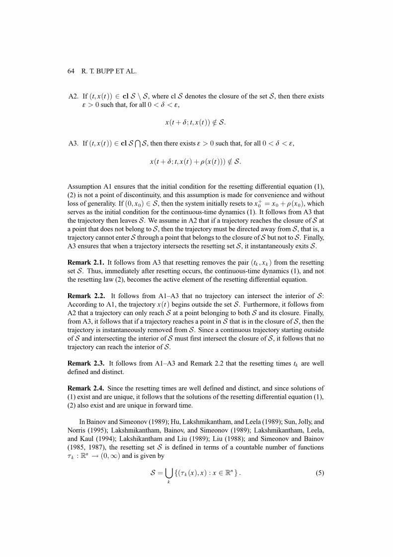
)LJXUH �� 7KLV SORW VKRZV WKH WLPH KLVWRU\ RI WKH HQHUJ\ FRPSRQHQWV IRU WKH RVFLOODWRU FRQWUROOHG E\

D WLPH�GHSHQGHQW UHVHWWLQJ YLUWXDO DEVRUEHU� 6LQFH WKHUH DUH QR GDVKSRW HOHPHQWV LQ WKH FORVHG�ORRS

V\VWHP� WKH WRWDO HQHUJ\ �GDVKHG OLQH� LV FRQVWDQW EHWZHHQ UHVHWWLQJ HYHQWV� DQG WKH LQFUHDVH LQ WKH

HPXODWHG HQHUJ\ �VROLG OLQH� HTXDOV WKH GHFUHDVH LQ SODQW HQHUJ\ �GDVK�GRW OLQH�� :KHQ D UHVHWWLQJ HYHQW

RFFXUV� ZKLFK IRU WKLV H[DPSOH LV HYHU\ � VHFRQG� WKH HPXODWHG HQHUJ\ LV LQVWDQWDQHRXVO\ UHVHW WR ]HUR�

ZKLOH WKH SODQW HQHUJ\ LV XQFKDQJHG�

It can be seen in (52) that the resetting law (49) causes the total energy to instantaneouslydecrease by an amount equal to the accumulated emulated energy.

To illustrate the dynamics of the closed-loop system, let pf @ 4, nf @ 4, and iwn j @i4> 5> 6> = = =j so that the controller resets periodically with a period of 1 second. The responseof the oscillator with the resetting virtual absorber to the initial condition t+3, @ 3, bt+3, @ 4,tf+3, @ 3, btf+3, @ 3 is shown in Figure 3. The energy in the oscillator is effectivelydissipated with an average rate of energy dissipation comparable to a 25% damping ratio.Note that the control force, illustrated in the lower plot of Figure 3, is discontinuous at theresetting times, but not impulsive.

A comparison of the plant energy, emulated energy, and total energy is given in Figure 4.It can be seen that, between resetting events, the total energy is constant, while any increasein the emulated energy is accompanied by a decrease in the plant energy. When a resettingevent occurs, the emulated energy is reset to zero, while the plant energy is unchanged.

In this example, the controller parameters and resetting times were chosen arbitrarily.However, a method for choosing the parameterspf and nf so as to achieve finite settling timefor this single-degree-of-freedom oscillator is described in Bupp et al. (1996). We considerthis approach in the following example.


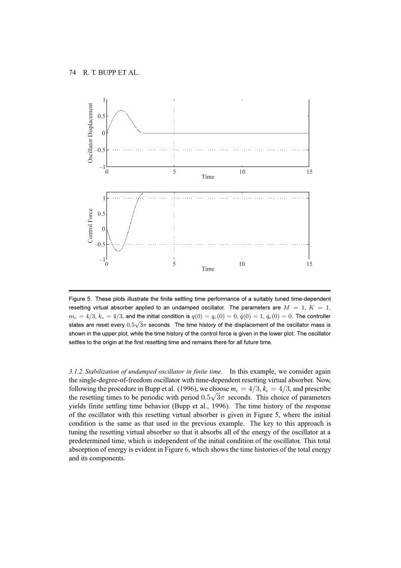
)LJXUH �� 7KHVH SORWV LOOXVWUDWH WKH ILQLWH VHWWOLQJ WLPH SHUIRUPDQFH RI D VXLWDEO\ WXQHG WLPH�GHSHQGHQW

UHVHWWLQJ YLUWXDO DEVRUEHU DSSOLHG WR DQ XQGDPSHG RVFLOODWRU� 7KH SDUDPHWHUV DUH � ' �� g ' ��

6S ' e*�� &S ' e*�� DQG WKH LQLWLDO FRQGLWLRQ LV Êf� ' ^SEf� ' f� �̂Ef� ' �� ̂SEf� ' f� 7KH FRQWUROOHU

VWDWHV DUH UHVHW HYHU\ f�DI�Z VHFRQGV� 7KH WLPH KLVWRU\ RI WKH GLVSODFHPHQW RI WKH RVFLOODWRU PDVV LV

VKRZQ LQ WKH XSSHU SORW� ZKLOH WKH WLPH KLVWRU\ RI WKH FRQWURO IRUFH LV JLYHQ LQ WKH ORZHU SORW� 7KH RVFLOODWRU

VHWWOHV WR WKH RULJLQ DW WKH ILUVW UHVHWWLQJ WLPH DQG UHPDLQV WKHUH IRU DOO IXWXUH WLPH�

3.1.2. Stabilization of undamped oscillator in finite time. In this example, we consider againthe single-degree-of-freedom oscillator with time-dependent resetting virtual absorber. Now,following the procedure in Bupp et al. (1996), we choosepf @ 7@6, nf @ 7@6, and prescribethe resetting times to be periodic with period 3=8

s6� seconds. This choice of parameters

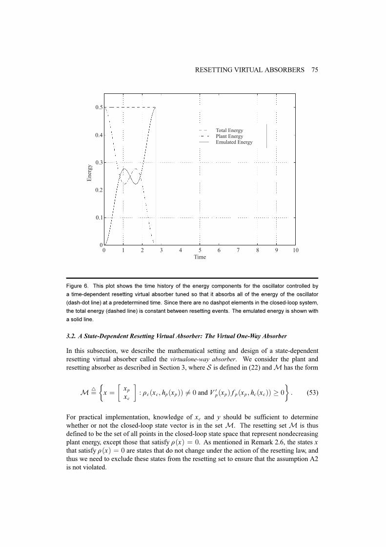
yields finite settling time behavior (Bupp et al., 1996). The time history of the responseof the oscillator with this resetting virtual absorber is given in Figure 5, where the initialcondition is the same as that used in the previous example. The key to this approach istuning the resetting virtual absorber so that it absorbs all of the energy of the oscillator at apredetermined time, which is independent of the initial condition of the oscillator. This totalabsorption of energy is evident in Figure 6, which shows the time histories of the total energyand its components.


)LJXUH �� 7KLV SORW VKRZV WKH WLPH KLVWRU\ RI WKH HQHUJ\ FRPSRQHQWV IRU WKH RVFLOODWRU FRQWUROOHG E\

D WLPH�GHSHQGHQW UHVHWWLQJ YLUWXDO DEVRUEHU WXQHG VR WKDW LW DEVRUEV DOO RI WKH HQHUJ\ RI WKH RVFLOODWRU

�GDVK�GRW OLQH� DW D SUHGHWHUPLQHG WLPH� 6LQFH WKHUH DUH QR GDVKSRW HOHPHQWV LQ WKH FORVHG�ORRS V\VWHP�

WKH WRWDO HQHUJ\ �GDVKHG OLQH� LV FRQVWDQW EHWZHHQ UHVHWWLQJ HYHQWV� 7KH HPXODWHG HQHUJ\ LV VKRZQ ZLWK

D VROLG OLQH�

3.2. A State-Dependent Resetting Virtual Absorber: The Virtual One-Way Absorber

In this subsection, we describe the mathematical setting and design of a state-dependentresetting virtual absorber called the virtualone-way absorber. We consider the plant andresetting absorber as described in Section 3, where V is defined in (22) andP has the form

P 7@

�{ @

�{s

{f

�= �f+{f > ks+{s,, 9@ 3 and Y 3s+{s, i s+{s > kf+{f,, � 3

�= (53)

For practical implementation, knowledge of {f and | should be sufficient to determinewhether or not the closed-loop state vector is in the set P. The resetting set P is thusdefined to be the set of all points in the closed-loop state space that represent nondecreasingplant energy, except those that satisfy �+{, @ 3. As mentioned in Remark 2.6, the states {that satisfy �+{, @ 3 are states that do not change under the action of the resetting law, andthus we need to exclude these states from the resetting set to ensure that the assumption A2is not violated.


By resetting the states, the plant energy can never increase. Also, if the continuous-time dynamics of the closed-loop system are lossless, then a decrease in plant energy isaccompanied by a corresponding increase in emulated energy. Hence, this approach allowsplant energy to òòflowóó to the controller, where it increases the emulated energy but doesnot allow the emulated energy to òòflowóó back to the plantñhence the name virtual one-wayabsorber.

We assume as before that if { 5 P, then { . �+{, @5 P. We further assume that if{ 5P, then

Yf+{f . �f+{f > |,> |, � Yf+{f> |,> (54)

and thus

Y +{ . �+{,, � Y +{,> (55)

so that, if (25) is satisfied, then Lyapunov (resp. asymptotic) stability of the closed-loopsystem follows from Theorem 2.2.

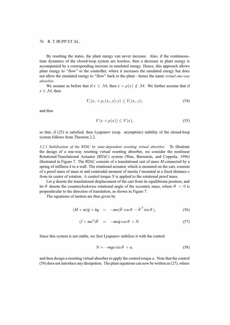
3.2.1. Stabilization of the RTAC by state-dependent resetting virtual absorber. To illustratethe design of a one-way resetting virtual resetting absorber, we consider the nonlinearRotational/Translational Actuator (RTAC) system (Wan, Bernstein, and Coppola, 1996)illustrated in Figure 7. The RTAC consists of a translational cart of mass P connected by aspring of stiffness n to a wall. The rotational actuator, which is mounted on the cart, consistsof a proof mass of mass p and centroidal moment of inertia L mounted at a fixed distance hfrom its center of rotation. A control torque Q is applied to the rotational proof mass.

Let t denote the translational displacement of the cart from its equilibrium position, andlet � denote the counterclockwise rotational angle of the eccentric mass, where � @ 3 isperpendicular to the direction of translation, as shown in Figure 7.

The equations of motion are thus given by

+P.p,�t. nt @ �ph+�� frv � � b�5vlq � ,> (56)

+L. ph5,�� @ �ph�t frv � . Q= (57)

Since this system is not stable, we first Lyapunov stabilize it with the control

Q @ �pjh vlq � . x> (58)

and then design a resetting virtual absorber to apply the control torque x. Note that the control(58) does not introduce any dissipation. The plant equations can nowbewritten as (27), where


)LJXUH �� 7KH URWDWLRQDO�WUDQVODWLRQDO DFWXDWRU PRGHO�

{ @

5997

{s4{s5{s6{s7

6::8 @

5997

tbt�b�

6::8 > i s+{s > x, @

59999997

bt

+L.ph5,+ph b�5�nt,�ph frv �x

+P.p,+L.ph5,�+ph frv �,5

b�

ph frv �+nt�ph b�5vlq �.+P.p,x

+P.p,+L.ph5,�+ph frv �,5

6::::::8= (59)

We will require as output the position and velocity of the rotational degree of freedom,

| @

��b�

�= (60)

The plant energy corresponds to the sum of the kinetic energies of the cart mass and the proofmass, the potential energy stored in the spring n, and the potential energy function associatedwith (58). Consequently,

Ys+{s, @4

5+P.p, bt5 .

4

5+L.ph5, b�

5.ph bt b� frv � .

4

5nt5 .pjh+4� frv � ,> (61)

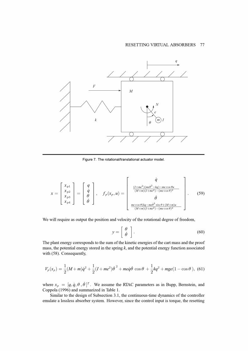
where {s @ ^t> bt> � > b� `W . We assume the RTAC parameters as in Bupp, Bernstein, andCoppola (1996) and summarized in Table 1.

Similar to the design of Subsection 3.1, the continuous-time dynamics of the controlleremulate a lossless absorber system. However, since the control input is torque, the resetting


7DEOH �� 6XPPDU\ RI 57$& SDUDPHWHUV�

Cart Mass P 65.50 ozArm Mass p 2.28 ozSpring Constant n 18.60 oz/inEccentricity h 2.43 inArm Inertia L 0.74 oz-in

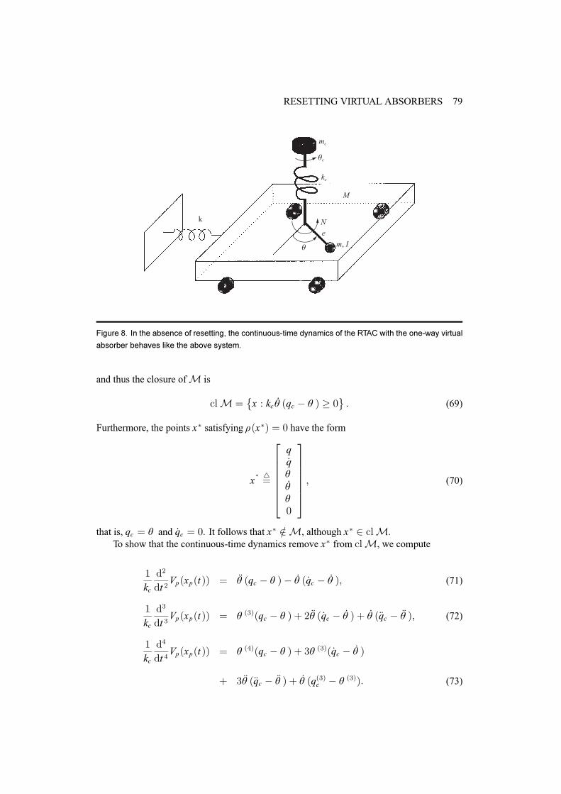
virtual absorber subsystem is based on the emulation of rotational spring and inertia elements.Consequently, the continuous-time dynamics of the closed-loop system behave like thesystem shown in Figure 8.

The resetting virtual absorber controller design is thus given by

{f @

�{f4{f5

�@

�tfbtf

�> i f+{f> |, @

�{f5

� nfpf

+{f4 � � ,

�>

kf+{f > |, @ nf+{f4 � � ,> (62)

Yf+{f > |, @4

5nf+{f4 � � ,5 .

4

5pf{

5f5> (63)

�{f @ �f+{f > � , @

�� {f4�{f5

�= (64)

We assume the initial condition of the controller to be

{f+3, @

�� +3,3

�= (65)

The resetting set (53) becomes

P7@�{ = �f+{f> � , 9@ 3 and nf b� +tf � � , � 3

�= (66)

Since �f+{f+3,> � +3,, @ 3, it is clear from (65) and (66) that assumption A1 is satisfied, thatis, {+3, @5P.

To show that assumption A2 holds in this case, we show that upon reaching anonequilibrium point {+w , @5 P that is in the closure ofP, the continuous-time dynamicsremove {+w , from clP, and thus necessarily move the trajectory a finite distance away fromP. If {+w , @5P is an equilibrium point, then

{+v, @5P> v � w> (67)

which is also consistent with assumption A2.Note that

g

gwYs+{s+w ,, @ nf b� +w ,+tf+w ,� � +w ,,> (68)


)LJXUH �� ,Q WKH DEVHQFH RI UHVHWWLQJ� WKH FRQWLQXRXV�WLPH G\QDPLFV RI WKH 57$& ZLWK WKH RQH�ZD\ YLUWXDO

DEVRUEHU EHKDYHV OLNH WKH DERYH V\VWHP�

and thus the closure ofP is

foP @�{ = nf b� +tf � � , � 3

�= (69)

Furthermore, the points {� satisfying �+{�, @ 3 have the form

{� 7@

59999997

tbt�b��3

6::::::8> (70)

that is, tf @ � and btf @ 3. It follows that {� @5P, although {� 5 foP.To show that the continuous-time dynamics remove {� from foP, we compute

4

nf

g5

gw 5Ys+{s+w ,, @ �� +tf � � ,� b� + btf � b� ,> (71)

4

nf

g6

gw 6Ys+{s+w ,, @ � +6,+tf � � , . 5�� + btf � b� , . b� +�tf � �� ,> (72)

4

nf

g7

gw 7Ys+{s+w ,, @ � +7,+tf � � , . 6� +6,+ btf � b� ,

. 6�� +�tf � �� , . b� +t+6,f � � +6,,= (73)


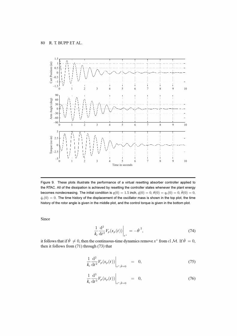
)LJXUH �� 7KHVH SORWV LOOXVWUDWH WKH SHUIRUPDQFH RI D YLUWXDO UHVHWWLQJ DEVRUEHU FRQWUROOHU DSSOLHG WR

WKH 57$&� $OO RI WKH GLVVLSDWLRQ LV DFKLHYHG E\ UHVHWWLQJ WKH FRQWUROOHU VWDWHV ZKHQHYHU WKH SODQW HQHUJ\

EHFRPHV QRQGHFUHDVLQJ� 7KH LQLWLDO FRQGLWLRQ LV Êf� ' ��D LQFK� �̂Ef� ' f� wEf� ' ^SEf� ' f� �wEf� ' f�

�̂SEf� ' f� 7KH WLPH KLVWRU\ RI WKH GLVSODFHPHQW RI WKH RVFLOODWRU PDVV LV VKRZQ LQ WKH WRS SORW� WKH WLPH

KLVWRU\ RI WKH URWRU DQJOH LV JLYHQ LQ WKH PLGGOH SORW� DQG WKH FRQWURO WRUTXH LV JLYHQ LQ WKH ERWWRP SORW�

Since

4

nf

g5

gw 5Ys+{s+w ,,

��{�

@ � b�5> (74)

it follows that if b� 9@ 3, then the continuous-time dynamics remove {� from foP. If b� @ 3,then it follows from (71) through (73) that

4

nf

g5

gw 5Ys+{s+w ,,

��{�> b�@3

@ 3> (75)

4

nf

g6

gw 6Ys+{s+w ,,

��{�> b�@3

@ 3> (76)


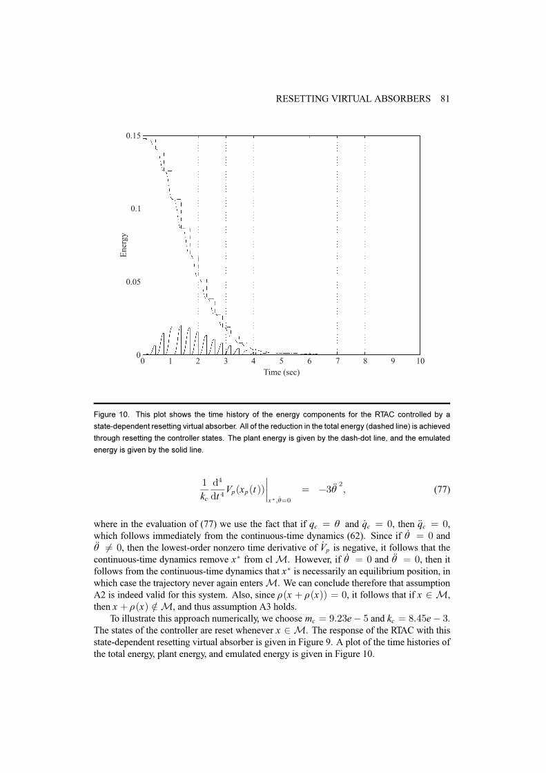
)LJXUH �� 7KLV SORW VKRZV WKH WLPH KLVWRU\ RI WKH HQHUJ\ FRPSRQHQWV IRU WKH 57$& FRQWUROOHG E\ D

VWDWH�GHSHQGHQW UHVHWWLQJ YLUWXDO DEVRUEHU� $OO RI WKH UHGXFWLRQ LQ WKH WRWDO HQHUJ\ �GDVKHG OLQH� LV DFKLHYHG

WKURXJK UHVHWWLQJ WKH FRQWUROOHU VWDWHV� 7KH SODQW HQHUJ\ LV JLYHQ E\ WKH GDVK�GRW OLQH� DQG WKH HPXODWHG

HQHUJ\ LV JLYHQ E\ WKH VROLG OLQH�

4

nf

g7

gw 7Ys+{s+w ,,

��{�> b�@3

@ �6�� 5> (77)

where in the evaluation of (77) we use the fact that if tf @ � and btf @ 3, then �tf @ 3,which follows immediately from the continuous-time dynamics (62). Since if b� @ 3 and�� 9@ 3, then the lowest-order nonzero time derivative of bYs is negative, it follows that thecontinuous-time dynamics remove {� from clP. However, if b� @ 3 and �� @ 3, then itfollows from the continuous-time dynamics that {� is necessarily an equilibrium position, inwhich case the trajectory never again entersP. We can conclude therefore that assumptionA2 is indeed valid for this system. Also, since �+{ . �+{,, @ 3, it follows that if { 5 P,then { . �+{, @5P, and thus assumption A3 holds.

To illustrate this approach numerically, we choose pf @ <=56h� 8 and nf @ ;=78h� 6.The states of the controller are reset whenever { 5 P. The response of the RTAC with thisstate-dependent resetting virtual absorber is given in Figure 9. A plot of the time histories ofthe total energy, plant energy, and emulated energy is given in Figure 10.


4. CONCLUSIONS

In this paper, we have developed a general framework for describing resetting virtualabsorbers for control. Two types of resetting virtual absorbersñtime-dependent resettingvirtual absorbers and state-dependent resetting virtual absorbersñare fully developed, andexamples are given to illustrate the ability of these controllers to remove energy from linearand nonlinear vibrating systems. A remaining theoretical issue is the proof of asymptoticstability for systems whose continuous time dynamics are Lyapunov stable and whose resetlaw causes Y to strictly decrease at each resetting time, that is, (25) is satisfied with equalityand (26) is satisfied with strict inequality. Finally, while the paper focused on unforcedsystems, analysis of virtual resetting absorbers for systems with forcing remains a topic forfuture research.

Acknowledgments. The research of R. T. Bupp and D. S. Bernstein was supported in part by the Air Force

Office of Scientific Research under grants F49620-95-1-0019 and F49620-93-1-0502.

The research of V. S. Chellaboina andW. M.Haddadwas supported in part by the National Science Foundation

under Grant ECS-9496249 and the Air Force Office of Scientific Research under Grant F49620-96-1-0125.

REFERENCES

Bainov, D. D. and Simeonov, P. S., 1989, Systems with Impulse Effect, Ellis Horwood Series in Mathematics and itsApplications. Ellis Horwood Limited, England.

Bupp, R. T., Bernstein, D. S., Chellaboina, V., and Haddad, W. M., 1996, òòFinite settling time control of the doubleintegrator using a virtual trap-door absorber,óó in Proceedings of the IEEE Conference on Control Applications,Dearborn, MI, September, pp. 179-184.

Bupp, R. T., Bernstein, D. S., and Coppola, V. T., 1996, òòExperimental implementation of integrator backstepping andpassive nonlinear controllers on the RTAC testbed,óó in Proceedings of the IEEE Conference on Control Appli-cations, Dearborn, MI, September, pp. 279-284.

Bupp, R. T., Corrado, J. R., Coppola, V. T., and Bernstein, D. S., 1995, òòNonlinear modification of positive-real LQGcompensators for enhanced disturbance rejection and energy dissipation,óó in Proceedings of the American Con-trol Conference, Seattle, WA, June, pp. 3224-3228.

Den Hartog, J. P., 1956,Mechanical Vibrations, 4th edition, McGraw-Hill, New York.

Duquette, A. P., Tuer, K. L., and Golnaraghi, M. F., 1993, òòVibration control of a flexible beam using a rotational internalresonance controller, Part I: Theoretical development and analysis,óó Journal of Sound and Vibration ��, 41-62.

Frahm, H., 1909, òòDevice for damping vibration of bodies,óó U.S. Patent No. 989958.

Golnaraghi, M. F., Tuer, K. L., andWang, D., 1994, òòDevelopment of a generalized active vibration suppression strategyfor a cantilever beam using internal resonance,óó Nonlinear Dynamics �, 131-151.

Golnaraghi, M. F., Tuer, K. L., and Wang, D., 1995, òòTowards a generalized regulation scheme for oscillatory systemsvia coupling effects,óó IEEE Transaction on Automatic Control ��, 522-530.

Haddad, W.M., Bernstein, D. S., andWang, Y.W., 1994, òòDissipativeO2*O" controller synthesis,óó IEEE Transactionson Automatic Control ��, 827-831.

Haddad, W. M. and Chellaboina, V., 1997, òòNonlinear fixed-order dynamic compensation for passive systems,óó in Pro-ceedings of the American Control Conference, Albuquerque, NM, June, pp. 2160-2164.

Hu, S., Lakshmikantham, V., and Leela, S., 1989, òòImpulsive differential systems and the pulse phenomena,óó Journalof Mathematical Analysis and Applications ��, 605-612.

Juang, J. and Phan, M., 1992, òòRobust controller designs for second-order dynamic systems: A virtual passive ap-proach,óó Journal of Guidance, Control, and Dynamics ��(5), 1192-1198.


Kishimoto, Y., Bernstein, D. S., and Hall, S. R., 1995, òòEnergy flow control of interconnected structures: I. Modalsubsystems, II. Structural subsystems,óó Control Theory and Advanced Technology ��(4), 1563-1618.

Korenov, B. G. and Reznikov, L. M., 1993, Dynamic Vibration Absorbers: Theory and Technical Applications, Wiley,UK.

Kulev, G. K. and Bainov, D. D., 1989, òòStability of sets for systems with impulses,óó Bulletin of the Institute of Mathe-matics Academia Sinica ��(4), 313-326.

Lai, J. S. andWang, K.W., 1996, òòParametric control of structural vibrations via adaptable stiffness dynamic absorbers,óóJournal of Vibration and Acoustics ��, 41-47.

Lakshmikantham, V., Bainov, D. D., and Simeonov, P. S., 1989, Theory of Impulsive Differential Equations, volume 6of Series in Modern Applied Mathematics, World Scientific, Singapore.

Lakshmikantham, V., Leela, S., and Kaul, S., 1994, òòComparison principle for impulsive differential equations withvariable times and stability theory,óó Nonlinear Analysis, Theory, Methods and Applications ��(4), 499-503.

Lakshmikantham, V., Leela, S., and Martynyuk, A. A., 1989, Stability Analysis of Nonlinear Systems, Marcel Dekker,New York.

Lakshmikantham, V. and Liu, X., 1989, òòOn quasi stability for impulsive differential systems,óó Nonlinear Analysis,Theory, Methods and Applications ��(7), 819-828.

Liu, X., 1988, òòQuasi stability via Lyapunov functions for impulsive differential systems,óó Applicable Analysis ��,201-213.

Lozano-Leal, R. and Joshi, S. M., 1988, òòOn the design of dissipative LQG-type controllers,óó in Proceedings of theIEEE Conference on Decision and Control, Austin, TX, December.

Ormondroyd, J. and Den Hartog, J. P., 1928, òòThe theory of the dynamic vibration absorber,óó Transactions of the ASME��.

Ouceini, S. S. and Golnaraghi, M. F., 1996, òòExperimental implementation of the internal resonance control strategy,óóJournal of Sound and Vibration ��, 377-396.

Ouceini, S. S., Tuer, K. L., and Golnaraghi, M. F., 1995, òòRegulation of a two-degree-of-freedom structure using reso-nance,óó Journal of Dynamic Systems, Measurement and Control ��, 247-251.

Phan, M., Juang, J., Wu, S., and Longman, R.W., 1993, òòPassive dynamic controllers for nonlinearmechanical systems,óóJournal of Guidance, Control, and Dynamics ��(5), 845-851.

Quan, R. and Stech, D., 1996, òòTime varying passive vibration absorption for flexible structures,óó Journal of Vibrationand Acoustics ��, 36-40.

Siddiqui, S.A.Q. and Golnaraghi, M. F., 1996, òòNew vibration regulation strategy and stability analysis for a flexiblegyroscopic system,óó Journal of Sound and Vibration ��, 465-481.

Simeonov, P. S. and Bainov, D. D., 1985, òòThe secondmethod of Lyapunov for systems with an impulse effect,óó TamkangJournal of Mathematics ��(4), 19-40.

Simeonov, P. S. and Bainov, D. D., 1987, òòStability with respect to part of the variables in systems with impulse effect,óóJournal of Mathematical Analysis and Applications ��, 547-560.

Snowdon, J. C., 1968, Vibration and Shock in Damped Mechanical Systems, John Wiley, New York.

Sun, L. Q., Jolly, M. R., and Norris, M. A., 1995, òòPassive, adaptive and active tuned vibration absorbers - A survey,óóJournal of Vibration and Acoustics ��, 234-242.

Tuer, K. L., Golnaraghi, M. F., and Wang, D., 1994, òòRegulation of a lumped parameter cantilever beam via internalresonance using nonlinear coupling enhancement,óó Dynamics and Control �, 73-96.

Wan, C., Bernstein, D. S., and Coppola, V. T., 1996, òòGlobal stabilization of the oscillating eccentric rotor,óó NonlinearDynamics ��, 49-62.

Watts, P., 1883, òòOn a method of reducing the rolling in ships at sea,óó Transactions of the Institute of Naval Architecture��, 165-190.

Documents

Resetting Virtual Absorbers for Vibration Control Virtual Absorbers for Vibration Control ROBERT T. BUPP TRW S & EG Redondo Beach, CA 90278, USA DENNIS S. BERNSTEIN Department of Aerospace