The University of Manchester Research

Residential sorting and environmental externalities:

DOI:10.1111/jors.12162

Document VersionAccepted author manuscript

Link to publication record in Manchester Research Explorer

Citation for published version (APA):Thanos, S., Bristow, A. L., & Wardman, M. R. (2015). Residential sorting and environmental externalities: The caseof nonlinearities and stigma in aviation noise values. Journal of Regional Science, 55(3), 468-490.https://doi.org/10.1111/jors.12162

Published in:Journal of Regional Science

Citing this paperPlease note that where the full-text provided on Manchester Research Explorer is the Author Accepted Manuscriptor Proof version this may differ from the final Published version. If citing, it is advised that you check and use thepublisher's definitive version.

General rightsCopyright and moral rights for the publications made accessible in the Research Explorer are retained by theauthors and/or other copyright owners and it is a condition of accessing publications that users recognise andabide by the legal requirements associated with these rights.

Takedown policyIf you believe that this document breaches copyright please refer to the University of Manchester’s TakedownProcedures [http://man.ac.uk/04Y6Bo] or contact uml.scholarlycommunications@manchester.ac.uk providingrelevant details, so we can investigate your claim.

Download date:12. Dec. 2021

1

Residential Sorting and Environmental Externalities: the Case of Non-

linearities and Stigma in Aviation Noise Values

Sotirios Thanosi, Abigail L. Bristow

ii, Mark R. Wardman

iii.

ABSTRACT

This paper explores the sorting process in response to differing levels of aviation noise exposure in a

housing market. Spatiotemporal Hedonic Pricing (HP) and Stated Choice (SC) results reflect

nonlinearities and stigma. The HP models reveal nonlinear noise depreciation increasing from 0.40

to 2.38 percent per decibel as noise increases, while the SC noise values are lower in an area with

high long-term noise exposure. These nonlinearities are attributed to the spatial sorting of noise

tolerant individuals. HP results from the same “noisy” area show a “stigma” from noise during the

first year after the complete removal of aviation noise.

Keywords: Valuation of Environmental Effects, Aviation Noise, Sorting, Spatial econometrics,

Stigma, Spatio-Temporal Models

JEL classifications: R210, R410, C210, Q510, Q530

Please cite as:

Thanos, S., Bristow A. L., Wardman, M. R. (2015), Residential sorting and environmental

externalities: the case of non-linearities and stigma in aviation noise values. Journal of Regional

Science, 55(3): 468–490 http://onlinelibrary.wiley.com/doi/10.1111/jors.12162/abstract

The link above provides the final published form. This article may be used for non-commercial

purposes in accordance with Wiley Terms and Conditions for Self-Archiving.

Acknowledgements

We would like to thank EUROCONTROL Experimental Centre for funding this research and especially Ted Elliff

and Ian Fuller. We also owe thanks to Yiannis Kapanidis for his help with the GIS modeling.

i CEE, UCL Energy Institute, University College London, email: s.thanos@ucl.ac.uk, tel: +44 (0)20 3108 9323

ii School of Civil and Building Engineering, Loughborough University

iii Institute for Transport Studies, the University of Leeds

2

1. INTRODUCTION

Sorting1 is used in the economics literature as a metaphor for the partition of economic agents

across segments of a market, as determined by market forces. With regard to the choice of

dwelling location, households sort across neighborhoods in accordance to their preferences for

environmental externalities, social attributes, travel costs and budget constraints. Understanding

consumer heterogeneity can be especially important for policy relating to public goods and

externalities (Kuminoff et al., 2013).

This paper examines sorting in the context of aviation noise. Long term noise exposure can cause

health, economic and social problems (Berglund et al., 1999; Miedema, 2007), especially for the

6.9 million people in Europe who are exposed to aviation noise levels above 55 decibels

(European Environment Agency, 2010). Examining the issue from an environmental justice

angle, Sobbota et al (2007) find socioeconomic attributes such as income, education level and

ethnicity to be significant predictors of whether households locate in areas highly exposed to

aviation noise, which is consistent with the sorting paradigm. Hence, arriving at robust monetary

values for the cost of the aircraft noise externality is important in informing appraisal and policy.

Our theoretical framework is based on the assumption2 of preference heterogeneity regarding the

level of noise residents are prepared to accept. This creates self-selection pressures that result in

a sorting process, whereby few in the housing market are prepared to accept high aircraft noise

exposure. This sorting process would over time create pockets of more (and less) noise tolerant

consumers across space, reflecting the spatial distribution of aviation noise exposure. We would

therefore expect differentiated noise values in different residential areas, according to long-term

noise exposure. Hence, we can derive two research hypotheses. First, residents in very “noisy”

areas will place lower values on noise nuisance. Second, a higher housing discount is required by

new entrants to these areas, as fewer housing market consumers are prepared to accept high

aviation noise exposure. A corollary hypothesis is that house buyers and sellers form negative

associations for areas exposed to long-term extreme noise; associations that do not immediately

dissipate after the removal of noise. These negative associations can result in noise depreciation

to house prices or “stigma” that endures for a period after aviation noise has ceased. In this paper

3

we test these hypotheses by looking at values of noise depreciation in the housing market derived

by Hedonic Pricing (HP) techniques and the direct willingness to pay (WTP) for quietness

derived from Stated Choice (SC) exercises.

Identifying the value of aviation noise has traditionally relied upon HP techniques. A common

assumption found in the vast majority of HP studies is that of a constant percentage of house

price depreciation per decibel of noise, the Noise Depreciation Index (NDI) (Nelson, 2008).

There is no theoretical basis for this assumption, only computational convenience, and such an

assumption is not consistent with the spatial sorting process of households. A small number of

studies (Day et al., 2007; Andersson et al., 2010; Wilhelmsson 2000; Pommerehne, 1988) find

progressively higher values per decibel at increasing noise levels, which would be consistent

with a sorting process. A closely related issue is that NDI is highly sensitive to the noise

threshold3 used; with higher the depreciation rates being observed at higher thresholds

(Andersson et al. 2010; Cohen and Coughlin, 2008; Bjorner et al., 2003; Rich and Nielsen 2004;

Bateman et al., 2001; Lake et al., 1998, 2000) implying a nonlinear relationship, which again is

consistent with the spatial sorting process of households.

The behavioural aspect of sorting in relation to transport noise exposure has been explored in

Stated Preference4 (SP) studies. Arsenio et al. (2006) and Eliasson et al. (2002) found that

individuals with higher marginal values of noise tended to live in quieter home locations.

Similarly, Wardman and Bristow (2004) found that those who had taken some actions to

alleviate noise had higher values of further noise reduction. Conversely, Pommerehne (1988) and

Vainio (2001) report that the presence of insulation can reduce the willingness to pay for further

noise reduction, which is inconclusive with regard to our hypothesis. A few SP results are not

consistent with sorting; according to Faburel and Luchini, (2000) and Thune-Larsen, (1995)

noise values are higher for respondents exposed to higher noise levels. However, Thune-Larsen

(1995) excluded genuinely noise tolerant individuals, who were not at all annoyed, from the

estimation of noise values.

Stigma effects, or the enduring depreciation of housing prices after the removal of a negative

externality, have been documented in the literature, in cases of proximity to hazardous

4

infrastructure/facilities or criminal activities (Congdon-Hohman, 2013; Hite et al, 2001;

McCluskey and Rausser, 2003). However, this effect has not been examined with regard to

facilities producing noise externalities.

The research hypotheses are tested by employing data from a rare experimental context, the

Hellenikon Airport closure in Athens. First, we test for nonlinearities by the re-estimation of the

Thanos et al. (2012) HP model from before the airport closure using a flexible log-sum threshold

approach. The novelty of our approach lies in explicitly linking nonlinearities to thresholds in

noise valuation and accounting for spatial sorting of households at differing levels of noise

exposure. Second, we estimate spatiotemporal HP models for the post airport-closure period to

determine whether any stigma from aviation noise remains on house prices. These

spatiotemporal models are specified to capture changes in neighborhood quality. These models

also address the common misspecification in the literature (Salvi, 2008; Dekkers and Van der

Straaten 2009; Chalermpong, 2010; Andersson et al., 2010; Cohen and Caughlin 2008) of

treating house sales data as cross-sectional and ignoring their temporal dimension. A house sale

and its corresponding price are only observed at a specific location and distinct moment in time.

The arrow of time and the direction of causality are violated by ignoring this fact with significant

econometric shortcomings (Dubé and Legros, 2014; Smith, 2009). To the best of our knowledge

this is the first application in the context of noise nuisance examining stigma. Third, as far as we

are aware this is the first study to apply SC and HP experiments in the context of aircraft noise

removal providing a unique opportunity for a cross method comparison of values. Therefore, we

are able to test the research hypotheses from both a revealed and stated preference perspective,

looking for noise nuisance values of residents in very “noisy” areas and the housing discount

required by new entrants to these areas.

The paper is structured as follows. Section 2 reviews previous evidence on nonlinearities of

noise values, threshold selection and stigma. Section 3 explains the log-sum approach to noise

threshold setting. Section 4 provides details about the Hellenikon airport closure context, data

and studies in the area. Section 5 presents the results of the pre-closure HP models on

nonlinearity of aviation noise. The methodological approach, the specification spatiotemporal

error models and results of the post-closure HP models are found in Section 6, focusing on

5

stigma. Section 7 brings together and discusses the monetary aircraft noise valuation estimates

from the SC, HP pre-closure and HP post-closure models. Conclusions are provided in Section 8.

2. REVIEW OF NONLINEARITY, THRESHOLDS AND STIGMA EVIDENCE

This section reviews cases of stigma in the housing market and the interconnected issues of

nonlinearities and thresholds in noise valuation studies.

Stigma in the housing market

Stigma effects in the housing market with regard to facilities producing noise externalities have

not been documented in the literature, although there are some examples of stigma from other

externalities. Congdon-Hohman (2013) looked at the stigma of crime represented by the

discovery of a methamphetamine laboratory in the vicinity, using a dataset on house sales in

Summit County, Ohio from 2002 to 2009. They found a 10-19 percent decrease in sale prices of

houses nearby in the year following a laboratory's discovery compared to those slightly further

away, suggesting some persistence of the effect which might be related to a continuing fear of

crime. Dale et al. (1999) examined the housing market from 1979 to 1995 around a lead smelter

in Dallas that was closed in 1984 and fully cleaned up by 1986. As expected, prices were

depressed during the smelter operational period but after the closure they increased across all

areas. However, locations closest to the smelter and poorer areas were slower to recover

suggesting some continuing effect. McCluskey and Rausser (2003) utilized the same example

but allowing the influence of the smelter to decline with distance. They suggest that long-term

stigma exists for properties within 1.2 miles of the site. Hite et al. (2001) found that long closed

landfill sites in Ohio have small but persistent effect on house prices in the vicinity. Hence, we

see examples of stigma effects in the literature having different duration, level of impact and

spatial distribution depending on the nature of the effect.

Nonlinearity of noise values and thresholds

The assumption of constant noise depreciation per decibel has been empirically examined by

only a handful of studies. Day et al. (2007) is the only paper to have applied the second stage HP

approach in noise valuation and estimated an inverse demand function for road traffic and rail

noise. They reported a range of increasing marginal prices for noise corresponding to increasing

6

noise levels. The average values for road noise varied appreciably from £31.49 per annum for a

1dBA reduction from a 56dBA baseline to £67.58 at 71dBA and £91.15 at 81dBA. Andersson et

al. (2010) specified a model with a pre-imposed nonlinear econometric relationship between

house prices and road noise. The model produced a NDI of 1.15 at 50dBA reaching 2.9 at

70dBA.

Wilhelmsson (2000) and Theebe (2004) also arrived at nonlinear NDI estimates, but with a

questionable statistical treatment of noise and arbitrary threshold assumptions. Wilhelmsson

(2000) uses two different variables for road noise simultaneously in the same model. The first is

for all observations having no noise threshold and the second variable includes only houses

visually exposed to a major road and a 68dBA threshold, which seems arbitrary after specifying

no threshold in the first variable. A nonlinear NDI is calculated combining both variables

without appropriate statistical significance tests for it5, even though only the second noise

variable is statistically significant. Theebe (2004) produces statistically significant estimates only

above 65dBA. The continuous noise data is converted to 5dBA band dummy variables that make

no distinction between observations within a noise contour/band. The noise banding imposes un-

testable assumptions about functional form of noise depreciation and thresholds.

As already described, a key issue across the noise valuation literature is that of the assumptions

used regarding noise thresholds. This is the level below which noise is assumed to impose no

nuisance and hence has no monetary value. The absence of cut-off points, as in Brandt and

Maenig (2011), is also problematic since it assumes that there is no other sound except the noise

source in the model. In HP studies of transport noise the threshold is traditionally set at around

50-55 dBA. Day et al. (2007) used a 55dBA threshold in their first stage HP model. However,

further analysis of their second stage results, reported in Nellthorp et al. (2007), suggested that

noise values were positive down to a 45dBA threshold. Andersson et al. (2010) specify a semi-

logarithmic spatial HP models at two threshold levels of 50 and 55dBA. In their subsequent

nonlinear model, they used a 50dBA cut-off and they pre-imposed a concave functional form to

this relationship.

7

There is some divergence in the literature about the significance and selection of noise thresholds

that is often treated as a matter of secondary importance. NDI is highly sensitive to the noise

threshold used, typically increasing when the threshold is set higher as illustrated in Table 1

where we reproduce results from studies using more than one threshold (Andersson et al. 2010;

Cohen and Coughlin, 2008; Bjorner et al., 2003; Rich and Nielsen 2002; Bateman et al., 2001

and Lake et al., 1998, 2000).

TABLE 1: Aviation and Road Noise Thresholds employed in recent HP studies

Authors Location Source Threshold

dBA

NDI

Lake et al. (1998,

2000)

Glasgow, Scotland Road 68

54

1.07

0.20

Bjørner et al. (2003) Copenhagen, Denmark Road 55 0.47

Rich and Nielson

(2004)

Copenhagen, Denmark

Road 50 Houses: 0.54

Flats: 0.47

Bateman et al. (2004) Birmingham, England Road 55 0.21-0.53

Theebe (2004) Western Netherlands Combined

transport

noise

65

dummy

specification

0.3 to 0.5

Baranzini and

Ramirez (2005)

Geneva, Switzerland, rental

sector

Road 50 0.25

Salvi (2008) Zurich, Switzerland Road

Aviation

50

50

0.82

0.97

Cohen and Coughlin

(2008)

Atlanta, US Aviation 65 dummy

70 dummy

NSSa

3.3

Dekkers and Van der

Straaten (2009)

Amsterdam, Netherlands Road

Aviation

Aviation

55

45

48

0.14

0.80

0.50

Andersson et al.

(2010)

Lerum, Sweden Road 50

55

1.15

1.69

Brandt and Maenig

(2011)

Hamburg, Germany Road

Aviation

None

62

0.23

0.13

Thanos et al. (2012) Athens, Greece Aviation 55 0.49 aNSS: not statistically significant at 95%

The only exception to this is the Dekkers and Van der Straaten (2009) study, where higher

thresholds reduced the aircraft noise depreciation and oddly the coefficient becomes insignificant

at a 50dBA threshold. They report a model with thresholds that vary by the noise source; 45dBA

for air traffic, 55dBA for road and 60dBA for rail. While the use of different thresholds attempts

to reflect evidence in the noise annoyance literature, it is questionable in this context. They are

8

effectively assuming that road traffic noise will not impact on welfare until it is 55dBA, whereas

aircraft noise will do so at half the intensity, 45dBA.

The threshold levels set for a single noise source should take account of the acoustic

environment. Bjørner et al. (2003) cautioned that their identification of 55dBA as threshold was

for a large urban area and that a lower level may be appropriate in a more rural environment.

Similarly, Thanos et al. (2011) found that a threshold of 55dBA gave the best fit to the urban

area data but that a lower threshold of 47dBA produced a better fit to data in more rural areas.

Evidence from other SP studies is sparse. Weinberger (1992) used a low cut off at 40dBA in a

Contingent Valuation study in Germany. Bristow and Wardman (2006) found that the model fit

deteriorated if a threshold was imposed, using aircraft valuation SC data from Lyon and

Manchester. Although limited, such SP evidence as there is appears to suggest lower or no

thresholds than those usually applied in HP.

While monetary noise values in HP are sensitive to thresholds, their selection is often arbitrary

and usually not tested. The threshold issue is closely connected to the hypothesis of nonlinear

noise depreciation: the higher the threshold the higher the NDI. We address this methodological

issue in Section 3, introducing the specification of a flexible log-sum threshold found in Thanos

et al., (2011, 2012), which also explicitly includes background noise levels.

3. THE LOG-SUM NOISE THRESHOLD APPROACH

The physical characteristics/properties of noise are important in the analysis and threshold

specification. Noise data are comprised of statistical indicators summarizing sound pressure

levels over time at the logarithmic scale of decibel (dB) units and a frequency weighting, “A” in

this case6 (Berglund et al., 1999). Transportation noise data, used in HP, are usually derived from

traffic flows (of trains, airplanes or road vehicles) through noise models, as taking actual noise

measurements over long periods of time in hundreds or thousands of locations would be

impractical. Hence, the available noise data often refer to specific noise sources and the average

overall noise levels for a large area might also be approximated.

9

Let us take the simplest case, where data are available for a specific noise source, say aviation γa.

The overall noise level γb from all other sources except aviation, henceforth termed background

noise, is also known. The issue with typical thresholds/cut-off points for a specific noise source

is that the noise variation in cross-sectional data is reduced as the threshold increases for that

source. This is because any observation below the threshold is assumed to be equal to the cut-off

point. For aviation noise, most of the observations in an affected area will exceed a 45dBA cut-

off point, but very few will exceed a 75 dBA cut-off. This lack of variation at higher cut-off

points (e.g. over 75dBA) causes the noise coefficients in HP models to be statistically

insignificant in any given dataset.

In HP models we want to capture the effect of aviation noise on the housing market above the

general noise level in the area, even for lower aviation noise levels, which is not possible with

typical cut-off points. Therefore, we follow Thanos et al. (2011, 2012) to define a total noise

level (γt), given by the combination of aviation noise level (γa) and the background noise level

(γb), as:

(1)

/10γ10

/10γ1010log)γ,(γγ ba

10bat .

If γa is dominant, γb will have an almost negligible effect on the total noise level and vice versa.

Equation 1 is commonly employed in the acoustics literature to calculate the sum of sound levels

from different sources (see Genescà et al., 2013). This has been completely overlooked in the

economics literature that addresses noise valuation, with the exception of Andersson et al.

(2010). However, they used Equation 1 to combine just rail and road noise levels to a “total”

noise level, and subsequently employed a typical cut-off point for the “total” noise level.

The threshold specification provided in Equation 1 has the advantage of including in the analysis

even low levels of aircraft noise that would otherwise have been below a certain cut off point.

Hence, by including all observations the log-sum thresholds do not reduce noise variation in

cross-sectional data, as typical cut-off points do. Furthermore, we take advantage of this property

of log-sum thresholds to examine nonlinearities, by determining the depreciation of house prices

due to aircraft noise for a range of thresholds between 45-75dBA. This is reported in Section 5.

10

4. THE AIRPORT CLOSURE CONTEXT AND DATA

Athens International Airport (AIA) or Hellenikon Airport operated for more than 40 years in the

southern suburbs of Athens, Greece. In March 2001, it was closed and the main Airport hub was

moved to the northeast of Athens. The population of the wider area affected at the airport by the

time of its closure was over 350,000, with a significant variation of aircraft noise exposure. The

following data types and approaches relevant to this context are presented here: aviation noise

data, the SC data and approach, the HP approach before the airport closure and housing data for

the post-closure period.

Aircraft noise data for Hellenikon Airport

The aircraft noise data for Hellenikon airport were supplied by the European Organization for

the Safety of Air Navigation (EUROCONTROL), who have complete data on flight paths and

aircraft movements for Hellenikon Airport. The consistency of the modelled data with actual

noise measurements was confirmed by EUROCONTROL. A set of coordinates for each house

sale or interview location was provided to EUROCONTROL and they supplied an estimate of its

aircraft noise exposure.

Thanos et al. (2011, 2012) employed the Lden7 noise metric, which is seen as appropriate for

aircraft noise in the EU (EC, 2002) and is commonly used in studies valuing noise (Dekkers and

Van der Straaten, 2009; Rich and Nielsen, 2004; Baranzini and Ramirez, 2005). Miedema et al.

(2000) investigated which noise metrics best predict annoyance from aircraft noise and supported

the use of weighted noise metrics, such as Lden, instead of Leq in this context.

Unfortunately, no data were available on other sources of noise pollution such as road traffic. We

follow Thanos et al. (2011, 2012) who set a 55dBA value for background noise γb, deduced from

previous studies of the noise situation in Athens that do not address aircraft noise (Nicol and

Wilson, 2004; Yang and Kang, 2005), and used the γt in Equation1 for aircraft noise in the HP

and SC models. In the SC experiment, the absence of aircraft noise is simply the background

noise level γb (Thanos et al., 2011).

11

SC around Hellenikon airport

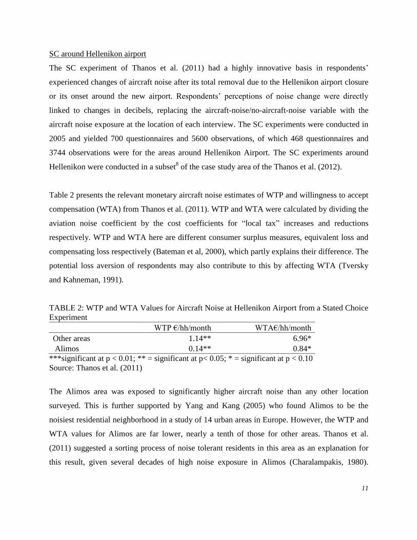
The SC experiment of Thanos et al. (2011) had a highly innovative basis in respondents’

experienced changes of aircraft noise after its total removal due to the Hellenikon airport closure

or its onset around the new airport. Respondents’ perceptions of noise change were directly

linked to changes in decibels, replacing the aircraft-noise/no-aircraft-noise variable with the

aircraft noise exposure at the location of each interview. The SC experiments were conducted in

2005 and yielded 700 questionnaires and 5600 observations, of which 468 questionnaires and

3744 observations were for the areas around Hellenikon Airport. The SC experiments around

Hellenikon were conducted in a subset8 of the case study area of the Thanos et al. (2012).

Table 2 presents the relevant monetary aircraft noise estimates of WTP and willingness to accept

compensation (WTA) from Thanos et al. (2011). WTP and WTA were calculated by dividing the

aviation noise coefficient by the cost coefficients for “local tax” increases and reductions

respectively. WTP and WTA here are different consumer surplus measures, equivalent loss and

compensating loss respectively (Bateman et al, 2000), which partly explains their difference. The

potential loss aversion of respondents may also contribute to this by affecting WTA (Tversky

and Kahneman, 1991).

TABLE 2: WTP and WTA Values for Aircraft Noise at Hellenikon Airport from a Stated Choice

Experiment

WTP €/hh/month WTA€/hh/month

Other areas 1.14** 6.96*

Alimos 0.14** 0.84*

***significant at p < 0.01; ** = significant at p< 0.05; * = significant at p < 0.10

Source: Thanos et al. (2011)

The Alimos area was exposed to significantly higher aircraft noise than any other location

surveyed. This is further supported by Yang and Kang (2005) who found Alimos to be the

noisiest residential neighborhood in a study of 14 urban areas in Europe. However, the WTP and

WTA values for Alimos are far lower, nearly a tenth of those for other areas. Thanos et al.

(2011) suggested a sorting process of noise tolerant residents in this area as an explanation for

this result, given several decades of high noise exposure in Alimos (Charalampakis, 1980).

12

Hence, there is scope to examine the variation of HP monetary values in Alimos and compare

with these results.

Pre-closure HP analysis and results

Thanos et al. (2012) applied spatiotemporal HP models on 1613 house sales from 1995 to 2001,

while Hellenikon airport was operational. Their novel specification of spatiotemporal HP models

is further discussed in section 6. They obtained statistically significant coefficients for aircraft

noise and an NDI estimate of 0.493.

Post-closure Housing Data

This study employs 773 observations of house sales starting immediately after the Hellenikon

airport closure on the 2nd quarter of 2001 to the end of 2003. Table 3 presents the data including

information about the basic structural characteristics of each house, such as the square meters of

floor space, construction year, sale date, number of rooms, presence of a garage, floor number

and house type. The full address of each house sale allowed the use of GIS to estimate additional

geographical information. Frankel (1988) and Bateman et al. (2001) found local amenities to

influence house prices. A number of amenity locations were acquired and the straight distance

between each house and the nearest school, city square, public service facility, and park/sport-

facility was calculated.

The distance from each house to the airport was also estimated. Even though there is no longer

an airport, there may still be disamenities from an abandoned airport or amenities as there were

plans to convert part of the site to a park and it housed many venues for the 2004 Olympic

Games. It is noted that due to the geography of the area (see Fig. 2, Thanos et al 2012) the spatial

variation of noise does not coincide with distance to the airport in our data (correlation

coefficient: 0.033). As the housing data here is for the post airport closure period, there is no

aircraft noise in the area around the old airport. Therefore, to test for any remaining stigma from

aircraft noise, we employ noise data from the last year of Hellenikon Airport operation in 2000.

13

TABLE 3: Post-Closure Data description

Variable Description Mean S.D. Min Max

price Mean house sale price in € in 2003

levels 252034 181603 50201 1235814

Ln_price Natural Logarithm of the house price 12.24 0.61 11 14

room_no Number of rooms 3.73 1.31 1 9

built_per Time elapsed in years since

construction of building 3.22 2.83 1 18

floor_no floor number 2.12 1.51 0 7

Aviation_noise dBA Lden of aviation noise 62.36 7.02 45.3 83.6

Total_noise The log-sum of aircraft(dBA Lden) and

background (55dBA) noise 63.84 5.56 55 84

Noise_Alimos As above only for Alimos area 67.27 6.12 56 82

Noise_No_Ali

mos As above for all areas except Alimos

62.90 5.01 55 84

sq meters Square meters of the house floor 94.37 58.51 21 470

room1_2 Dummy equals 1 when 1 or 2 rooms 0.17 0.37 0 1

room3 Dummy equals 1 when 3 rooms 0.25 0.43 0 1

room4 Dummy equals 1 when 4 rooms 0.39 0.49 0 1

room5 Dummy equals 1 when 5 rooms 0.06 0.23 0 1

room6 Dummy equals 1 when 6 rooms 0.05 0.23 0 1

room7 Dummy equals 1 when 7 rooms or over 0.05 0.22 0 1

House>10yr Dummy equals 1 when house built over

10years 0.06 0.23 0 1

House 6-9yr Dummy equals 1 when house built

between 6 and 9 years ago 0.08 0.28 0 1

H_Age_B Dummy equals 1 when the house age is

below 5 years or unknown 0.86 1.00 0 1

floors_7-8 Dummy equals 1 when floor num. 7-8 0.00 0.06 0 1

floors_4-6 Dummy equals 1 when floor num. 4- 6 0.18 0.39 0 1

floors<4 Dummy equals 1 when floor number is

below 4 or unknown 0.82 0.97 0 1

detached Dummy equals 1 when detached house 0.04 0.19 0 1

Semi_ter Dummy equals 1 when semidetached or

terraced house 0.04 0.20 0 1

Flat Dummy equals 1 when flat 0.92 1.94 0 1

garage Dummy equals 1 when private garage 0.30 0.46 0 1

d_parks Distance in meters to the nearest park or

outdoor sporting facility 576 335 21 1676

d_public_serv Distance in meters to the nearest public

service building 540 333 14 1865

d_plaza Distance in meters to the nearest plaza 360 207 14 1168

d_school Distance in meters to the nearest school 368 254 14 1699

d_airport Distance in meters to the airport 5061 2454 497 10760

y2001-y2003 Dummies for each year from 2001 to 2003

14

As expected, Alimos exhibits significantly higher aircraft noise levels compared to the other

study areas in Table 3. We create two interaction variables between aircraft noise and Alimos

area to capture noise effects specific to this area. The first (Noise_Alimos) contains the total

noise level (γt) of house sales only in Alimos, keeping all other house sales at the background

noise (γb) level of 55dBA. The second (Noise_No_Alimos) is the reverse, containing only the

background noise (γb) for Alimos house sales and the total noise level including aircraft (γt) for

all other areas.

5. NONLINEARITY OF THE NDI

As discussed in Section 3, the log-sum threshold specification in Equation1 does not reduce

noise variation at higher noise levels as much as typical cut-off points do. We exploit this

property to examine nonlinearities by determining the depreciation of house prices due to aircraft

noise that exceeds a range of thresholds from 45dBA to75dBA.

The aircraft noise data used in Thanos et al. (2012) is appropriate for this exercise as it exhibits a

wide noise variation. We exactly replicate the preferred HP model of Thanos et al. (2012),

diverging only in the aircraft noise variable specification. The model with a 55 dBA threshold,

which is considered the average background value for all the areas around the old airport, is

identical to that reported in Thanos et al. (2012).

An iterative process was adopted by varying the threshold value (γb) in equation 1 from 45 to 75

dBA and estimating separate HP model for each threshold value (γb) and resulting total noise

level (γt). This should be looked at as filtering process, consistent with sorting, that is dominated

by the aviation noise (γa) values that exceed each threshold (γb) level. It is noted that aviation

noise (γa) varies from 38 – 82 dBA. The results from the log-sum threshold specification are

compared to results by identical models that employ the typical cut-off points.

Table 4 presents the NDI estimates from our iterative modelling process. Our preferred results

correspond with the relationship previously assumed by Andersson et al. (2010); the relationship

identified between noise exposure and house prices is indeed concave, as the NDI increases

convexly (see Figure 1). A one dBA increase in noise levels would cause house prices to fall by

15

0.4 percent at 45 dBA but by 2.38 percent at 75 dBA. The rate increases slowly until the noise

level reaches around 65 dBA when the rate of increase becomes more rapid. This nonlinearity is

consistent with the sorting; new buyers require discounts that increase nonlinearly in

progressively noisier locations.

TABLE 4: Comparison of pre-closure HP results with Log-sum and Typical Cut-off Thresholds

Threshold Level HP results with log-sum thresholds HP results with typical cut-off point thresholds

dBALden NDI za NDI 95% Conf. Int. Final LL NDI z

a NDI 95% Conf. Int. Final LL

45 0.4025 -3.64 0.6194 0.1856 235.73 0.3823 -3.60 0.5905 0.1740 235.81

46 0.4069 -3.64 0.6261 0.1877 235.67 0.3853 -3.60 0.5951 0.1754 235.78

47 0.4120 -3.64 0.6339 0.1901 235.61 0.3883 -3.60 0.6000 0.1766 235.73

48 0.4181 -3.64 0.6430 0.1932 235.54 0.3908 -3.59 0.6044 0.1772 235.66

49 0.4248 -3.64 0.6532 0.1963 235.45 0.3936 -3.58 0.6092 0.1780 235.59

50 0.4327 -3.65 0.6651 0.2002 235.36 0.3969 -3.57 0.6148 0.1790 235.51

51 0.4418 -3.65 0.6789 0.2047 235.26 0.4035 -3.59 0.6239 0.1830 235.50

52 0.4521 -3.66 0.6945 0.2097 235.14 0.4101 -3.60 0.6331 0.1871 235.48

53 0.4639 -3.66 0.7125 0.2154 235.01 0.4131 -3.59 0.6390 0.1873 235.31

54 0.4777 -3.66 0.7333 0.2220 234.87 0.4151 -3.54 0.6446 0.1856 235.03

55 0.4932 -3.66 0.7570 0.2293 234.70 0.4175 -3.49 0.6521 0.1829 234.65

56 0.5110 -3.67 0.7843 0.2378 234.52 0.4272 -3.47 0.6686 0.1858 234.36

57 0.5317 -3.67 0.8159 0.2474 234.33 0.4411 -3.46 0.6907 0.1915 234.08

58 0.5557 -3.67 0.8526 0.2587 234.13 0.4554 -3.45 0.7144 0.1964 233.74

59 0.5826 -3.66 0.8943 0.2709 233.90 0.4719 -3.42 0.7421 0.2018 233.34

60 0.6137 -3.66 0.9425 0.2848 233.65 0.4935 -3.40 0.7782 0.2088 232.94

61 0.6492 -3.65 0.9980 0.3004 233.39 0.5284 -3.40 0.8330 0.2238 232.66

62 0.6898 -3.63 1.0619 0.3177 233.11 0.5742 -3.40 0.9050 0.2434 232.39

63 0.7359 -3.61 1.1351 0.3368 232.82 0.6239 -3.36 0.9879 0.2600 231.95

64 0.7898 -3.59 1.2207 0.3589 232.52 0.6786 -3.30 1.0819 0.2753 231.41

65 0.8498 -3.56 1.3178 0.3818 232.18 0.6978 -3.05 1.1464 0.2492 230.26

66 0.9197 -3.52 1.4314 0.4080 231.85 0.6969 -2.72 1.1995 0.1943 228.98

67 0.9982 -3.47 1.5613 0.4352 231.49 0.6948 -2.39 1.2642 0.1253 227.86

68 1.0896 -3.42 1.7134 0.4657 231.13 0.7211 -2.16 1.3755 0.0666 227.10

69 1.1949 -3.36 1.8910 0.4988 230.76 0.7775 -2.00 1.5399 0.0152 226.59

70 1.3178 -3.30 2.0998 0.5357 230.40 0.8319 -1.79 1.7410 -0.0772 226.06

71 1.4645 -3.24 2.3498 0.5791 230.07 0.7878 -1.38 1.9051 -0.3296 225.31

72 1.6362 -3.18 2.6458 0.6266 229.74 0.6035 -0.84 2.0156 -0.8087 224.62

73 1.8377 -3.10 2.9976 0.6777 229.40 0.7284 -0.77 2.5768 -1.1200 224.50

74 2.0830 -3.04 3.4261 0.7399 229.11 1.0164 -0.79 3.5232 -1.4904 224.46

75 2.3791 -2.98 3.9453 0.8129 228.84 1.5391 -0.84 5.1169 -2.0387 224.46 a The z value refer to the coefficients in the regression

16

Looking at the final log-likelihood, the overall fit to the data is reduced with increasing

thresholds in both specifications. This is expected as essentially each model is placing increasing

constraints on the data, thus reducing noise variation. It is stressed that this not an exclusive

characteristic to our data, it is an inherent property of the estimation. Data from other studies

would produce similar results when estimating models with different cut-off thresholds, as in

Dekkers and Van der Straaten (2009) study higher cut-offs reduced the statistical significance of

noise aircraft noise depreciation, losing significance at 50dBA.

The comparison between the log-sum threshold and a typical cut-off specification is quite

interesting, clearly demonstrating the superiority of the log-sum threshold approach. The

difference between the two specifications to overall goodness of fit is trivial at lower noise

levels, but markedly increases in favor of the log-sum specification especially above 65dBA. The

NDIs from the log-sum threshold models have higher statistical significance across the whole

range of thresholds. As expected, NDI from the typical cut-off specification increase with

increasing thresholds and is closer to the NDI values from log-sum specification at lower

thresholds. At higher threshold levels, especially above 50dBA, this difference becomes more

pronounced. At the same time, the cut-off model NDIs become more “noisy” and at 67 dBA and

70dBA lose statistical significance at the 99 and 95 percent level respectively. The NDI

significance in log-sum threshold model is highest at 56-58dBA, compared to 45-47 dBA in the

cut-off threshold models.

These issues amply demonstrate the weakness of the typical cut-off specification, especially at

higher noise levels. In principle, the log-sum threshold approach could be extended to combine

noise from multiple noise sources and account for the general soundscape (and even introduce

variation across areas) in a more realistic manner to typical cut-off points where such data is

available.

6. STIGMA

Having established nonlinearities in house price depreciation from aircraft noise, the next step is

to determine whether any stigma remains after the removal of the noise externality. Furthermore,

we can also examine whether nonlinearity is an issue here as well. We have therefore estimated

17

models with housing data in the post-closure period to examine the stigma hypothesis from

aircraft noise and any nonlinearities.

Methodology and Spatiotemporal Considerations

HP posits that the price of a composite commodity, housing in this case, is a function of its utility

bearing attributes. The slope of the HP function can be used to determine the consumer’s WTP

for a given attribute, such as noise. A house sale and its corresponding price are only observed at

a specific location and distinct moment in time. Henceforth, the house sale data are called

spatiotemporal data and it is stressed that this is not panel data nor cross-sectional.

Indeed, subjecting spatiotemporal data to the “cross-sectional” treatment and ignoring the

temporal dimension is the common approach in recent spatial econometric HP papers that value

noise (Salvi, 2008; Dekkers and Van der Straaten 2009; Chalermpong, 2010; Andersson et al.,

2010; Cohen and Caughlin 2008). This misspecification produces a symmetric spatial weight

matrix S, given in equation 2,

(2) s𝑖𝑗 = {𝑓(d𝑖𝑗) if 𝑖 ≠ 𝑗

0 if 𝑖 = 𝑗 ,

where house sales/prices simultaneously influence each other weighted by a function of distance

d. Hence, future sales/prices are taken to influence past sale/prices, which violates the laws of

physics. House prices are time-variant and information about future prices cannot possibly travel

backwards in time, hence Spatial Autoregressive (SAR) models9 are not appropriate for

spatiotemporal data. Furthermore, future house prices cannot and should not be taken as proxies

of current expectations for the future, as current expectations are only shaped by information in

the present/past, amply demonstrated by the recent housing crisis.

The following argument for the Spatial Error Model (SEM) application to spatiotemporal data

has been put forward: SEM is supposed to be capturing time-invariant spatially distributed errors

affecting the IID10

properties of the regression residuals. Nevertheless, it makes no sense to use

the symmetric spatial weight matrix to account for time-invariant spatial errors in spatiotemporal

data. A spatially weighted error term in HP only captures spatially distributed unobserved effects

specifically from other house sales. Therefore, unobserved effects of house sales in the future

18

cannot affect house prices in the past. Time-invariant unobserved effects influence both past and

future in the same way. Hence, these time-invariant effects should not be accounted for by

spatially weighting HP residuals of house sales that have not happened yet, but by an additional

separate time-invariant error term. This is a significant avenue for future research (Smith and

Wu, 2009), but beyond the scope of this paper.

Imposing a “cross-sectional” treatment to spatiotemporal data produces an over-connected

spatial weight matrix, in which all observations simultaneously influence each other. Smith

(2009) demonstrated that the presence of strongly connected spatial weight matrices introduces

serious biases into both the testing and estimating of spatial dependence. These biases have been

found to erroneously subsume coefficient estimates of genuinely exogenous effects (Dubé and

Legros, 2014; Thanos et al., 2012; Bateman et al. 2004). The effects of overlooking or miss-

representing the temporal dimension of spatiotemporal data is the focus of an emerging body of

spatial econometrics literature (Smith and Wu, 2009; Nappi-Choulet and Maury, 2009, 2011;

Huang et al., 2010; Dubé and Legros, 2013a, 2013b, 2014; Dubé et al., 2014; Thanos et al.,

2012).

We adopt the approach of Thanos et al. (2012), also followed in the pre-closure models. The

spatiotemporal weight matrix W is specified to include both spatial and temporal distance. Each

element in matrix W is the product of the spatial sij and temporal tij distance between each pair of

observations (house sales), as given respectively in equation 3:

(3)

𝑠𝑖𝑗 = �

𝑑𝑖𝑗−1 ∀ 𝑑𝑖𝑗 τi ≻ τj ∧ i ≠ j

1 ∀ 𝑑𝑖𝑗 = 0 ∧ i ≠ j

0 ∀𝑑𝑖𝑗 τi ≼ τj ∨ i = j

,

and equation 4:

(4) 𝑡𝑖𝑗 = �

(ξi − ξj)–1

∀ (ξi − ξj) > 0 ∧ i ≠ j

1 ∀ ξi = ξj ∧ i ≠ j

0 ∀ (ξi − ξj) < 0 ∨ i = j

.

19

dij is simply the Euclidean distance between i and j. τi and τj are the sale dates of houses i and j

respectively. The spatial distance effects are only included in W when the sale of house i

succeeds the sale of house j. When the data are ordered chronologically, W is a lower triangular

matrix. Only sales in the past affect subsequent sales and not vice versa. ξ is an appropriate time

metric, quarter in this case (see Thanos et al. 2012), starting at the earliest observation in the

data. Hence, ξi − ξj captures the time elapsed between the observations i and j.

SAR and SEM are transformed to Spatiotemporal Autoregressive (STAR) model and

Spatiotemporal Error Model (STEM) respectively, given that spatiotemporal instead of spatial

weight matrices are employed. The differences also extend to how the coefficients of the

spatiotemporal effects are interpreted. STAR captures unidirectional spatial spillovers only from

past observations, instead of the multidirectional endogenous effects in SAR. STAR can include

technological and/or pecuniary spillovers, but the spatial multiplier discussed in Small and

Steimetz (2012) is not applicable here, since the spillovers are unidirectional.

The STEM specification applied house sales data captures a specific effect different to STAR or

SEM11

. STEM addresses the special case of either a new-built house j or an

improvement/deterioration to house j after its last sale. Both cases impose to all future sales an

externality φ* that is not fully captured in the own price of house j. A simile for the externality

imposed by new-built houses can be road traffic congestion, where each extra car imposes

external cost to all others on the road. The construction of an extra house affects all other houses

in the area improving or deteriorating the current neighborhood quality, as do major house

improvements/deteriorations. Even purely from a dwelling density perspective φ* is not

necessarily negative, as a marginal increase in dwelling density may be negative in some

markets/areas and positive in others depending on existing density (Dunse, et al., 2013).

Therefore, φ* can include a positive agglomeration externality (Thanos and White, 2014) or

negative “overcrowding” externality. The only study seen employing STEM in HP is Thanos et

al., (2012) and their data is mostly comprised of new-build houses. Even though they do not fully

discuss the issue of φ*, their results suggest that φ* is a positive externality in that context.

20

A crucial methodological issue is the selection of either STAR or STEM, given their differences.

The appropriate test for detecting spatial/spatiotemporal dependence is Moran’s I and for

selecting the model form are the locally robust variations of the Lagrange Multiplier (LM) test

(Anselin et al., 1996; Franzese and Hays, 2008). Table 5 presents these tests, where the null

hypothesis in Moran’s I test of no spatial/spatiotemporal dependence is rejected. The test for

STEM is highly significant while the robust STAR test is not. This means that houses prices are

not significantly affected by other house prices nearby, but by the developing urban structure of

the area and house improvements or the introduction of new-build houses in the urban

environment. This makes sense for this specific market, since here has been significant new

development in the area during the study period evident by 49.2 percent of the houses sold being

newer than 2 years of age. It is also shown that the model selection tests between SAR and SEM

are inconclusive, which was also observed in Thanos et al. (2012).

Given the LM test results we select the STEM. Its structural form is shown in equation 5 and its

reduced form in equation 6:

P is a vector of the house prices12

, Z is a matrix of housing characteristics and b is a vector of the

coefficients. λ is the spatiotemporal error coefficient, capturing the spatiotemporal distance

weighted (W) error effect ε. Externality φ* of the unobserved change in neighborhood quality is

captured by λ.

TABLE 5: Spatial Dependence diagnostics

Spatial weight Spatiotemporal Weight

Statistic p-value Statistic p-value

Moran's I 7.827 0 4.940 0

Lagrange multiplier: SEM/STEM 24.389 0 11.000 0.001

Robust Lagrange multiplier: SEM/STEM 17.476 0 11.235 0.001

Lagrange multiplier: SAR/STAR 17.938 0 0.135 0.714

Robust Lagrange multiplier: SAR/STAR 11.024 0.001 0.370 0.543

(5) 𝐏 = 𝐙𝐛 + ε, ε = 𝜆𝐖𝜀 + 𝑢, u ~ N(0, σ²I),

(6) 𝑢 = [𝐈 − 𝜆𝐖]𝐏 − [𝐈 − 𝜆𝐖] 𝐙𝐛.

21

Post-closure Model Results

The post-closure HP models’ results are found in Table 6. Most of the coefficients are of the

expected sign and consistent with the results of the pre-closure model in Thanos et al. (2012),

even though our sample size is significantly lower. The spatiotemporal error coefficient λ is

positive and statistically significant showing a positive unobserved change in neighborhood

quality, in agreement with Thanos, et al (2012). Our focus is on aircraft noise and we do not

discuss other effects, except to say that the distance to the airport still has a statistically

significant positive coefficient even after its closure, which captures the proximity disamenities

to an abandoned airport.

Housing market stigma effects were reviewed in Section 2, but we have not identified any

studies on stigma effects relating to transportation noise. The first of the two models reported

here (STEM1) includes an aircraft noise variable for the whole area which shows, as expected,

no negative effect or stigma. We tested for nonlinearities in stigma values. However, the

statistical significance13

of the aircraft noise coefficient is not improved even when we use the

iterative log-sum threshold approach in Section 5 to look at higher levels of noise exposure.

Noise stigma in Alimos

Given that stigma is not attached to isolated observations of high noise exposure, we tested

instead whether stigma is attached to certain areas as a whole. Alimos is the obvious choice,

given the high noise exposure and the scope to examine the variation of HP noise values there,

stressed in section 3. In the STEM2 model (Table 6), the aircraft noise variable is statistically

significant only for Alimos. This suggests that everywhere else, except Alimos, the negative

effect of aircraft noise disappeared along with the airport closure. The model indicates a house

price depreciation of 0.31 percent per dBA in Alimos for aircraft noise exposure that has now

ceased.

22

TABLE 6: The Post-closure Models

Model STEM 1 STEM 2: Alimos

STEM 3: Alimos

attenuating stigma

Variable Name Coef. Coef.

Total_noise -0.0026

Noise_Alimos

-0.0031**

Noise_No_Alimos

-0.0024 -0.0009

Noise_Alimos_y01 -0.0027***

Noise_Alimos_y02 -0.0001

sq meters 0.0053*** 0.0054*** 0.0054***

room1_2 -0.5728*** -0.5730*** -0.5706***

room3 -0.2429*** -0.2431*** -0.2411***

room4 Base Base Base

room5 0.1223*** 0.1224*** 0.1208***

room6 0.2354*** 0.2351*** 0.2392***

room7 0.2588*** 0.2584*** 0.2574***

House>10yr -0.0727** -0.0734** -0.0693**

House 6-9yr -0.0349 -0.0354 -0.0331

H_Age_B Base Base Base

floors_7-8 0.0113 0.0098 0.0112

floors_4-6 0.0942*** 0.0935*** 0.0930***

floors<4 Base Base Base

detached 0.2241*** 0.2243*** 0.2245***

Semi_ter -0.0965** -0.0971** -0.0948**

flat Base Base Base

garage 0.1080*** 0.1083*** 0.1089***

d_ parks -9.27E-05*** -9.34E-05*** -8.86E-05***

d_public_serv 5.37E-05** 5.46E-05** 5.32E-05**

d_plaza -1.26E-04*** -1.24E-04*** -1.29E-04***

d_school 1.45E-04*** 1.44E-04*** 1.51E-04***

d_airport 9.79E-06*** 9.62E-06*** 8.86E-06***

y2001 -0.1609*** -0.1601***

y2002 -0.0110 -0.0101

y2003 Base Base

constant 12.07*** 12.22*** 11.95***

λ 0.0183*** 0.0251*** 0.01937***

Wald χ2(48) 6315.94*** 6317.29*** 6277.98***

Final LL 147.713 147.798 145.649

***significant at p < 0.01; ** = significant at p< 0.05

23

This is an extraordinary finding, but at the same time it would be unreasonable to expect that this

effect would persist indefinitely14

. Therefore, we introduce interaction variables between

Noise_Alimos and the yearly dummies15

to STEM3 model. The results in Table 6 show that

indeed this effect attenuates after 2001 and only during that year there is a depreciation of 0.27

percent per dBA in Alimos. The interpretation of this finding is that the negative associations (in

the perceptions of buyers and sellers) for “noisy” Alimos, formed over decades of heavy noise

exposure, persist during 2001 and dissipate after that. This could be a behavioral effect and/or

inefficiencies in that housing market not allowing instantaneous adjustments after the removal of

severe noise exposure. We have no way to distinguish between these effects from our current

data.

For completeness, we also test if there are any area effects in Alimos prior to the airport closure.

The Alimos/No-Alimos interaction variables were inserted to the pre-closure model of Thanos et

al. (2012) to test any peculiar area effects. An asymptotic t-test16

showed that the aircraft noise

depreciation in Alimos is not significantly different at the 95 percent from all other areas in the

pre-closure model.

7. STIGMA, NONLINEARITIES AND SPATIAL SORTING

The HP and SC values are converted to a €/dBA/year form to facilitate discussion of the

similarities, differences and implications and consistency with the sorting process. The price at

which the household purchases a property can be considered as the discounted sum of all the

future per period rents from the property. Hence, the monetary value of house attributes may be

expressed per period, say annually, to be comparable with SC values. Appendix 1 illustrates in

detail the approach and assumption of converting NDI to an annual stream.

Figure 1 plots the curve of aircraft noise monetary values from this study over the range of 45 to

75dBA. This curve is very close to linear below 60dBA, with the nonlinearity becoming more

pronounced above the 66-68dBA levels. The curves for the monetary values of road traffic noise

from Andersson et al. (2010) and Day et al. (2007) are also plotted, as there are no comparable

aircraft noise values over such a detailed range of noise exposure levels in the literature. The

dotted lines illustrate the linear approximation of the curves. The second stage HP model of Day

24

et al. (2007) produces values that increase linearly with the noise levels. The findings of

Andersson et al. (2010) for road traffic noise show monetary noise values per dBA to be less

convex (flatter) than our findings. It is stressed that our approach tested independently for

nonlinearity without any imposition of a curve shape.

Table 7 presents the results of SC experiments, pre-closure and post-closure HP models. The

uncompensated Marshalian HP value is not directly comparable to income compensated welfare

values of WTP and WTA from the SC experiment. The range of value estimates from SC

experiment in the base category seem to “envelop” aircraft noise value estimates from HP,

except in the case of Alimos. The SC WTP and WTA values for Alimos are extremely low. For

example, Alimos residents would be willing to pay very little for aircraft noise not to return,

about eight times less than the other residents around Hellenikon airport. It is not credible that

other factors, such as income differentials, would explain this difference.

Both the HP and SC results are consistent with the sorting process framework. The nonlinear HP

noise values capture the higher discount required by the new entrants to the housing market in

noisier locations. The SC values of current residents in the noisiest location, Alimos, are

markedly lower than other areas. There are also negative associations in housing consumers’

perceptions that manifest into a localized stigma only in Alimos that endures for the first year

after the airport closure.

TABLE 7: Monetary Valuesa of Aircraft Noise from HP and SC Models

SC WTP SC WTA HP pre-closure HP post-closure:

Stigma during 2001

Other areas €15.78 €96.34 €55.52 not significant

Alimos €1.94 €11.63 €50.04 €26.09 a All values in this table are in €/dBA/year at 2003 price levels (Eurostat, 2012)

25

FIGURE 1: Comparison of the annuala monetary value

b (€) of one decibel change.

a Andersson et al (2010) NDI results were converted to €/dBA/year as indicated in Appendix 1

b All values in this Figure are in €/dBA/year PPP adjusted at 2003 price levels (Eurostat, 2012)

8. CONCLUSIONS

Preference heterogeneity with regard to noise exposure provides the theoretical framework of

households sorting across dwelling locations with different exposure levels. This process causes

a differentiation in noise values derived from different segments of consumers, according to the

spatial distribution of noise exposure. More detailed hypotheses in support of sorting were

derived for the direction of HP and SC values changes at differing levels of aviation noise

exposure, along with the corollary hypothesis of stigma. Our results are consistent with these

hypotheses. In the pre-closure HP models, new housing market entrants were found to require

discounts that increased convexly in progressively noisier locations. The SC noise values of

current residents in Alimos, a special case with significantly higher long-term aviation noise

This paper, Aviation

Noise

Andersson et al, Road

Noise

Day et al,Road Noise

0

50

100

150

200

250

45 46 47 48 49 50 51 52 53 54 55 56 57 58 59 60 61 62 63 64 65 66 67 68 69 70 71 72 73 74 75

26

exposure, are considerably lower than SC values from other areas and HP values in the same

area. Alimos is also the only area subject to stigma or unalleviated house price depreciation for

the first year after the complete removal of aviation noise, possibly due to enduring negative

associations in housing market participants’ perceptions and/or inefficiencies in that housing

market not allowing instantaneous adjustments after the removal of severe noise exposure.

A state-of-the-art STEM was employed to address the common misspecification in spatial HP

studies of ignoring the temporal dimension of spatiotemporal data and violating the arrow of

time. The positive and statistically significant spatiotemporal error coefficient captures the

unobserved improvement in neighborhood quality that includes the positive externality of adding

an extra house in the urban environment.

To the best of our knowledge, this is the first time the theoretical framework of the sorting

process has been applied to noise valuation. More importantly, this theoretical framework

predicts the divergence between the direction of HP and SC noise values in noisy areas, HP

increasing and SC decreasing. Another novelty is the recovery of a local noise stigma for the first

time in the literature. This is also the first time that NDI nonlinearities have been explicitly

linked to threshold selection and the underlying soundscape. The nonlinearity in aircraft noise

monetary values before the airport closure is comprehensively explored by an iterative modeling

procedure across a range of noise levels. A flexible log-sum threshold approach is utilized that

does not reduce noise variation in cross-sectional data. This approach may be extended to

combine noise from multiple sources and account for variations in the soundscape of different

areas in a more realistic manner to typical cut-off points or thresholds. The NDI ranges from 0.40

to 2.38 per dBA for dwellings exposed to aircraft noise exceeding 45dBA and 75dBA

respectively, indicating a convex relationship.

These findings have implications for noise valuation and policy. First, low noise value estimates

from SC and other types of SP applications should be treated with caution, especially where

populations are subject to self-selection pressures as a result of long term noise exposure and

sorting. There is a need to assess risks to health of such exposure in such communities. Second,

where a constant value per decibel is applied in appraisal noise costs will be under-estimated.

27

This is particularly true of areas with high levels of noise exposure, given the nonlinear

depreciation of house prices per dBA of noise increase. Third, the costs from an environmental

externality such as noise may well continue after its complete removal, especially in highly

exposed areas.

A few avenues of further research stem from this paper. One could be the extension of this

approach to equilibrium sorting models that incorporate changes in the supply side of the

housing market and a robust framework for valuing non-marginal changes. The design and

application of SP experiments that further test the spatial sorting of noise tolerant households

would be interesting, especially if specified to incorporate the nonlinearities in values. Another

avenue would be improvements in the specification of log-sum thresholds and studies that

combine more noise sources, explicitly taking into account the soundscape of the study areas.

28

1 It is noted that the approaches of formal “equilibrium sorting” models are not followed here due to data

constraints. 2 Along with the typical assumptions of homebuyer rationality, efficient housing markets, no transaction

costs and exogenously determined aviation noise. 3 This is the noise level below which noise is assumed to have no monetary value.

4 We use SP as an overarching term to include both SC, contingent valuation, and other types of

choice/ranking experiment. It is used when the implications discussed go further than SC and are relevant

to all SP type of studies 5 The test of both coefficients being jointly statistically different from zero is not appropriate. The NDI is

a linear combination of two coefficients with different variances and a covariance. The variance of NDI

should be estimated to conduct tests of statistical significance (Hole, 2007). 6 A-weighting is the frequency weighting operating as a close proxy to human auditory sensitivity as a

function of frequency (Lee and Fleming 2002). 7 Equivalent continuous sound pressure level over a fixed time period (Leq), where the evening values

(18:00 – 22:00) are weighted by the addition of 5 dBA (A-weighted decibel), and the night values (22:00

– 06:00) are weighted by the addition of 10 dBA 8 Municipalities of Alimos, Palaio Faliro, Glyfada and Hellenikon

9 where the hedonic price function of each house includes spatially weighted lagged prices of other houses

10 Independent and identically distributed

11 Let us take two house sales, j that precedes house sale i. It seems reasonable that the effect φ from

house j should be in the spatiotemporal error term if it influences house price i, but cannot be controlled

for by the researcher. However, if φ is observed by the buyer of house i and influences its price, it is

reasonable to assume it was also observed by the buyer of house j that is the source of φ. Hence, the effect

φ has already been captured in the price of house j and this would require a STAR specification capturing

a technological spillover. Hence, STEM can only capture own unobserved effects that either did not affect

the price of j or took place after the sale of j (and before house sale i). 12

Given that the Box–Cox specification is not readily implemented in the presence of spatial dependence

(Kim et al., 2003), a semi-log specification is selected. 13

The z-values for 45dBA and 65dBA are 1.65 and 1.85 respectively, not closer to 95 percent level

significance than the 55dBA (z: 1.87). The statistical significance drops further above 65dBA. 14

We are grateful to the two anonymous referees for pointing this out. 15

We have dropped the yearly dummies due to severe multicollinearity: Variance inflation (VIF) for

Noise_Alimos*y2001=122.13; Noise_Alimos*y2002 VIF=75.48; y2001 VIF=121.89; and y2002

VIF=74.99. However, we are confident that “Noise_Alimos*y2001” term does not capture the y2001

dummy effect, if anything these two variables are negatively correlated. The correlation between “y2001”

and “Noise_Alimos” is -0.0857. We cannot reject the null hypothesis of “y2001” and “Noise_Alimos”

being independent (Spearman's rho = -0.0536, Prob > |t| = 0.1365)

16 ),(2)()(/ 212

2

1

2

21 t = 0.98, where β1 is the aircraft noise coefficient for

Alimos and β2 is the noise coefficient for all other areas.

29

REFERENCES

Andersson, Henrik, Lina Jonsson, and Mikael Ögren. 2010. “Property Prices and Exposure to

Multiple Noise Sources: Hedonic Regression with Road and Railway Noise,” Environmental and

Resource Economics, 45, 73–89.

Anselin, Luc, Anil K.Bera, Raymond Florax, and Mann J. Yoon. 1996. “Simple Diagnostic Tests

for Spatial Dependence,” Regional Science and Urban Economics, 26, 77–104.

Arsenio, Elisabete, Abigail L. Bristow, and Mark Wardman. 2006. “Stated Choice Valuations of

Traffic Related Noise,” Transportation Research D, 11, 15-31.

Bank of Greece. 2007. Monthly Statistical Bulletins. Athens Greece: Economic Research

Department, Bank of Greece.

Baranzini, Andrea and José V. Ramirez. 2005. “Paying for Quietness: The Impact of Noise on

Geneva Rents,” Urban studies, 42, 633–646.

Bateman, Ian J., Ian H. Langford, Munro Alistair, Starmer Chris, and Robert Sugden. 2000.

“Estimating Four Hicksian Welfare Measures For A Public Good: A Contingent Valuation

Investigation,” Land Economics, 76(3), 355–373.

Bateman, Ian J., Brett Day, Iain Lake, and Andrew Lovett. 2001. “The Effect of Road Traffic

Noise on Residential Property Values: A Literature Review and Hedonic Pricing Study,”

Scottish Executive Development Department, Edinburgh, UK.

Bateman, Ian J., Brett Day, and Iain Lake. 2004. “The Valuation Of Transport-Related Noise in

Birmingham,” Non-technical report to Department for Transport, University of East Anglia, UK.

Berglund, Birgitta, Thomas Lindvall, and Dietrich H. Schwela. 1999. Guidelines for Community

Noise, Expert Task Force Meeting Guideline Document. Geneva: World Health Organization.

Bjørner, Thomas B., Jacob Kronbak, and Thomas Lundhede. 2003, “Valuation of Noise

Reduction–Comparing Results from Hedonic Pricing and Contingent Valuation,” SØM

Publication, no. 51. Copenhagen, Denmark: AKF Forlaget.

Brandt, Sebastian and Wolfgang Maennig. 2011. “Road Noise Exposure and Residential

Property Prices: Evidence from Hamburg,” Transportation Research Part D: Transport and

Environment, 16, 23-30.

30

Charalampakis, Grigoris. 1980. “Κοινωνική Έρευνα Γύρω από το Διεθνές Αεροδρόμιο

Αθηνών,” (A Social Survey around Athens International Airport) Αρχιτεκτονική Ακουστική και

Πολεοδομική Ηχοπροστασία (Architectural Acoustics and Urban Noise Protection), 2, 209 – 215

(article in Greek).

Chalermpong, Saksith. 2010. “Impact of Airport Noise on Property Values: Case of

Suvarnabhumi International Airport, Bangkok, Thailand,” Journal of the Transportation

Research Board, 2177, 8–16.

Cohen, Jeffrey P. and Cletus C. Coughlin. 2008. “Spatial Hedonic Models of Airport Noise,

Proximity, and Housing Prices,” Journal of Regional Science, 48, 859–878.

Congdon-Hohman, Joshua M. 2013. “The Lasting Effects of Crime: The Relationship of

Discovered Methamphetamine Laboratories and Home Values,” Regional Science and Urban

Economics, 43, 31-41.

Day, Brett, Ian J. Bateman, and Iain Lake. 2007. “Beyond Implicit Prices: Recovering

Theoretically Consistent and Transferable Values for Noise Avoidance from a Hedonic Property

Price Model,” Environmental and Resource Economics, 37, 211–232.

Dale, Larry, James C. Murdoch, Mark A. Thayer, and Paul A. Waddell. 1999. “Do Property

Values Rebound from Environmental Stigmas? Evidence from Dallas,” Land Economics, 75,

311-326.

Dekkers, Jasper E.C. and J. Willemijn van der Straaten. 2009. “Monetary Valuation of Aircraft

Noise: A Hedonic Analysis around Amsterdam Airport, Ecological Economics, 68, 2850–2858.

Dubé, Jean, Diègo Legros, Marius Thériault, and François Des Rosiers. 2014. “A spatial

Difference-in-Differences Estimator to Evaluate the Effect of Change in Public Mass Transit

Systems on House Prices,” Transportation Research Part B: Methodological, 64, 24-40.

Dubé, Jean and Diègo Legros. 2013a. “A Spatio-Temporal Measure of Spatial Dependence: An

Example Using Real Estate Data,” Papers in Regional Science, 92, 19–30.

Dubé, Jean and Diègo Legros. 2013b. “Dealing with Spatial Data Pooled Over Time in

Statistical Models,” Letters in Spatial and Resource Sciences, 6, 1-18.

Dubé, Jean and Diègo Legros. 2014. “Spatial Econometrics and the Hedonic Pricing Model:

What about the Temporal Dimension?” Journal of Property Research.

Dunse, Neil A., Sotirios Thanos, and Glen Bramley. 2013. “Planning Policy, Housing Density

and Consumer Preferences,” Journal of Property Research, 30, 221-238.

31

Eliasson, Jonas, Johanna Lindqvist Dillen, and Jenny Widell. 2002. “Measuring Intrusion

Valuations through Stated Preference and Hedonic Prices: A Comparative Study,” paper

presented at the European Transport Conference, London.

European Environment Agency, 2010. Towards a Resource-Efficient Transport System, TERM

2009: Indicators Tracking Transport and Environment in The European Union, No2/2010.

Copenhagen, Denmark: European Environment Agency.

European Council, 2002. “Directive 2002/30/EC of the European Parliament and of the Council

of 26 March 2002 on The Establishment of Rules And Procedures with Regard to the

Introduction of Noise-Related Operating Restrictions at Community Airports”, Official Journal

of the European Communities L, 85/40, P. 0040 - 0046.

Eurostat, 2012. Purchasing Power Parities, Price Level Indices and Real Expenditures, unit G6.

Luxembourg: The Statistical Office of the European Union.

Faburel Guillaume and Stephane Luchini. 2000. “The Social Cost of Aircraft Noise: The

Contingent Valuation Method Applied to Paris-Orly Airport,” paper presented at the 29th

International Congress and Exhibition on Noise Control Engineering, Nice, France.

Frankel, Marvin. 1988. “Impact of Aircraft Noise on Residential Property Market,” Illinois

Business Review, 45, 8-13.

Franzese, Jr. Robert J. and Jude C. Hays. 2008. “Empirical Models of Spatial Interdependence,”

in a J. M. Box-Steffensmeier, H.E. Brady, and D. Collier (eds.), The Oxford Handbook of

Political Methodology. Oxford, UK: Oxford University Press, pp. 570-604.

Genescà, Meritxell, Jordi Romeu, Robert Arcos, and Sara Martín. 2013. “Measurement of

Aircraft Noise in a High Background Noise Environment Using a Microphone Array,”

Transportation Research Part D, 18, 70–77.

Hite,Diane, Wen Chern, Fred Hitzhusen, and Alan Randall. 2001. “Property-Value Impacts of an

Environmental Disamenity: The Case of Landfills,” Journal of Real Estate Finance and

Economics, 22(2), 185 – 202.

Hole, Arne Risa. 2007. “A Comparison of Approaches to Estimating Confidence Intervals for

Willingness to Pay Measures,” Health Economics, 16 (8), 827–840.

Huang, Bo, Wu Bo, and Barry Michael. 2010. “Geographically and Temporally Weighted

Regression for Modeling Spatiotemporal Variation in House Prices,” International Journal of

Geographical Information Science, 24(3), 383–401.

32

Kim, Chong Won, Tim T. Phipps, and Luc Anselin. 2003. “Measuring the Benefits of Air

Quality Improvement: A Spatial Hedonic Approach,” Journal of Environmental Economics and

Management, 45, 24–39.

Kuminoff, Nicolai V., V. Kerry Smith, and Christopher Timmins. 2013. "The New Economics of

Equilibrium Sorting and Policy Evaluation Using Housing Markets," Journal of Economic

Literature, 51(4), 1007-1062.

Lake, Iain R., Andrew Lovett, Ian J. Bateman, and Brett Day. 2000. “Improving Land

Compensation Procedures Via GIS And Hedonic Pricing,” Environment and Planning C:

Government and Policy, 18, 681 – 696.

Lake, Iain R., Andrew Lovett, Ian J. Bateman, and Ian H. Langford. 1998. “Modelling

Environmental Influences on Property Prices in an Urban Environment,” Computers,

Environment and Urban Systems, 22, 121-136.

Lee, Cynthia S.Y. and Gregg G. Fleming. 2002. “General Health Effects of Transportation

Noise,” US Department of Transportation.

McCluskey, Jill J., Gordon C. Rausser. 2003. “Stigmatized Asset Value: Is It Temporary or Long

Term?” Review of Economics and Statistics, 85 (2), 276-285.

Miedema, Henk M.E. 2007. “Annoyance Caused By Environmental Noise: Elements for

Evidence-Based Noise Policies,” Journal of Social Issues, 63, 41-57.

Miedema, Henk M.E., Vos Henk, and Ronald G. de Jong. 2000. “Community Reaction to

Aircraft Noise: Time-Of-Day Penalty and Trade off Between Levels of Overflights,” Journal of

the Acoustical Society of America, 107, 3245–3253.

Nappi-Choulet, Ingrid and Tristan-Pierre Maury. 2009. “A Spatiotemporal Autoregressive Price

Index for the Paris Office Property Market,” Real Estate Economics, 37(2), 305–340.

Nappi-Choulet, Ingrid and Tristan-Pierre Maury.2011. “A Spatial and Temporal Autoregressive

Local Estimation for the Paris Housing Market,” Journal of Regional Science, 51(4), 732–750.

Nellthorp, John, Abigail L. Bristow, and Brett Day. 2007. “Introducing Willingness-To-Pay for

Noise Changes into Transport Appraisal – An Application of Benefit Transfer,” Transport

Reviews 27(3) 327-353.

Nelson, Jon P. 2008. “Hedonic Property Value Studies of Transportation Noise: Aircraft and

Road Traffic,” in a A. Baranzini, J. Ramirez, C. Schaerer, and P. Thalmann (eds.), Hedonic

33

Methods in Housing Markets Pricing Environmental Amenities and Segregation. New York,

USA: Springer, pp. 55-82.

Nicol, Fergus and Michael Wilson. 2004. “The Effect of Street Dimensions and Traffic Density

on the Noise Level and Natural Ventilation Potential in Urban Canyons,” Energy and Buildings,

36, 423–434.

Pommerehne, Werner W. 1988. “Measuring the Environmental Benefits: A Comparison of

Hedonic Technique and Contingent Valuation,” in a D. Bos, M. Rose, and C. Seidl (eds.),

Welfare and Efficiency in Public Economics. Berlin: Springer-Verlag, pp. 363-400.

Rich, Jeppe H. and Otto A. Nielsen. 2004. “Assessment of Traffic Noise Impacts,” International

Journal of Environmental Studies, 61, 19–29.

Salvi, Marco. 2008. “Spatial Estimation of the Impact of Airport Noise on Residential Housing

Prices,” Swiss Journal of Economics and Statistics, 2008-IV-3, 577–606.

Smith, Tony E. 2009. “Estimation Bias in Spatial Models with Strongly Connected Weight

Matrices,” Geographical Analysis, 41, 307–332.

Smith, Tony E. and Peggy Wu. 2011. “A Spatio-Temporal Model of Housing Prices Based on

Individual Sales Transactions Over Time,” Journal of Geographical Systems, 11(4), 333–355.

Sobotta, Robin R., Heather E. Campbell, and Beverly J. Owens. 2007. “Aviation Noise and

Environmental Justice,” Journal of Regional Science, 47, 125-154.

Thanos, Sotirios, Abigail L. Bristow, and Mark R. Wardman. 2012. “Theoretically Consistent

Temporal Ordering Specification in Spatial Hedonic Pricing Models Applied to the Valuation of

Aircraft Noise,” Journal of Environmental Economics and Policy, 1, 103-126.

Thanos, Sotirios, Mark R. Wardman, and Abigail L. Bristow. 2011. “Valuing Aircraft Noise:

Stated Choice Experiments Reflecting Inter-Temporal Noise Changes from Airport Relocation,”

Environmental and Resource Economics, 50, 559-583.

Thanos, Sotirios and Michael White. 2014. “Expectation Adjustment in the Housing Market:

Insights from the Auction System in Scotland,” Housing Studies, 29 (3), 339-361.

Theebe, Marcel A. J. 2004. “Planes, Trains, And Automobiles: The Impact of Traffic Noise on

House Prices,” Journal of Real Estate Finance and Economics, 28, 209–234.

Thune-Larsen, Harald. 1995. “Flystøyavgifter Basert På Betalingsvillighet”, TØI rapport,

289/1995, Institute of Transport Economics, Norwegian Centre for Transport Research, Oslo.

34

Tversky, Amos and Daniel Kahneman. 1991. “Loss Aversion in Riskless Choice: A Reference-

Dependent Model,” The Quarterly Journal of Economics, 106(4), 1039-1061.

Vainio, Matti. 2001. “Comparison of Hedonic Price and Contingent Valuation Methods in the

Urban Traffic Noise Context,” paper presented at the 2001 International Congress and Exhibition

on Noise Control Engineering, The Hague.

Wardman Mark R. and Abigail L. Bristow. 2004. “Traffic Related Noise and Air Quality

Valuations: Evidence from Stated Preference Residential Choice Models,” Transportation

Research D, 9, 1-27.

Weinberger, Marius. 1992. “Gesamtwirtschaftliche Kosten des Lärms in der Bundesrepublik

Deutschland,” Zeitschrift für Lärmbekämpfung, 39, 91-99.

Wilhelmsson, Mats. 2000. “Impact of traffic Noise on the Values of Single-Family Houses,”

Journal of Environmental Planning and Management, 43, 799-815.

Yang, Wei and Jian Kang. 2005. “Acoustic Comfort Evaluation in Urban Open Public Spaces,”

Applied Acoustics, 66, 211–229.

35

APPENDIX 1: Converting NDI to annual monetary stream

We follow Bateman et al. (2004) who examine the relationship between rents and house prices.

They argue that their findings imply a discount rate that lies between the mortgage rate and the

deposit interest rate of the Central Bank. They also assume a certain degree of “myopia” on

behalf of house buyers. That is, households are assumed to calculate their discount rate based on

current interest rates. Bateman et al. (2004) also argue that it is mathematically convenient and

not too unrealistic to assume that the expected life of the property can be taken as infinite.

The central Bank of Greece (2007) 12-month time-deposits rates fell from 10.2 in 1997 and 8.7

in 1999 to 3.3 percent in 2001. The mortgage interest rate fell from 12.6 in 1999 to 6.5 percent in

2001 and it has been around 5 percent after 2002 (Bank of Greece, 2007). There is much

variability before 2001, which cannot be captured easily in a single discount rate. The “myopia”

assumption of Bateman et al (2004) might not be sufficient in this case, since the public knew

well in advance the effects on mortgage, deposit and inflation rates, of Greece entering the Euro-

zone. The discount rate of 5 percent is therefore considered more appropriate for calculating

annual values. It is not in the middle of the mortgage and the bank deposit rates, but closer to

mortgage rate, to account for higher discount rates before 2001 and for “myopia” on the part of

house buyers.

Multiplying the discounted annual rent by the noise depreciation, aircraft noise monetary values

in the form of €/dBA/year are obtained. All values in Tables 7 and Figure 1 are adjusted to 2003

price levels (Eurostat, 2012). The monthly values in Thanos et al. (2011) are converted to annual.