Resilient Aircraft Sustainment: Quantifying Resilience

Air Force Institute of Technology Air Force Institute of Technology

AFIT Scholar AFIT Scholar

Theses and Dissertations Student Graduate Works

3-26-2020

Resilient Aircraft Sustainment: Quantifying Resilience through Resilient Aircraft Sustainment: Quantifying Resilience through

Asset and Capacity Allocation Asset and Capacity Allocation

Zachary B. Shannon

Follow this and additional works at: https://scholar.afit.edu/etd

Part of the Management and Operations Commons, and the Operations and Supply Chain

Management Commons

Recommended Citation Recommended Citation Shannon, Zachary B., "Resilient Aircraft Sustainment: Quantifying Resilience through Asset and Capacity Allocation" (2020). Theses and Dissertations. 3205. https://scholar.afit.edu/etd/3205

This Thesis is brought to you for free and open access by the Student Graduate Works at AFIT Scholar. It has been accepted for inclusion in Theses and Dissertations by an authorized administrator of AFIT Scholar. For more information, please contact [email protected].

https://scholar.afit.edu/

https://scholar.afit.edu/etd

https://scholar.afit.edu/graduate_works

https://scholar.afit.edu/etd?utm_source=scholar.afit.edu%2Fetd%2F3205&utm_medium=PDF&utm_campaign=PDFCoverPages

http://network.bepress.com/hgg/discipline/1311?utm_source=scholar.afit.edu%2Fetd%2F3205&utm_medium=PDF&utm_campaign=PDFCoverPages



https://scholar.afit.edu/etd/3205?utm_source=scholar.afit.edu%2Fetd%2F3205&utm_medium=PDF&utm_campaign=PDFCoverPages

mailto:[email protected]

RESILIENT AIRCRAFT SUSTAINMENT: Quantifying Resilience through Asset

and Capacity Allocation

THESIS

Zachary B. Shannon

AFIT-ENS-MS-20-M-288

DEPARTMENT OF THE AIR FORCE AIR UNIVERSITY

AIR FORCE INSTITUTE OF TECHNOLOGY

Wright-Patterson Air Force Base, Ohio

DISTRIBUTION STATEMENT A. APPROVED FOR PUBLIC RELEASE; DISTRIBUTION UNLIMITED.

The views expressed in this thesis are those of the author and do not reflect the official policy or position of the United States Air Force, Department of Defense, or the United States Government. This material is declared a work of the U.S. Government and is not subject to copyright protection in the United States.


RESILIENT AIRCRAFT SUSTAINMENT: QUANTIFYING RESILIENCE THROUGH ASSET

AND CAPACITY ALLOCATION

THESIS

Presented to the Faculty

Department of Operational Sciences

Graduate School of Engineering and Management

Air Force Institute of Technology

Air University

Air Education and Training Command

In Partial Fulfillment of the Requirements for the

Degree of Master of Science in Logistics & Supply Chain Management

Zachary B. Shannon

March 2020

DISTRIBUTION STATEMENT A. APPROVED FOR PUBLIC RELEASE; DISTRIBUTION UNLIMITED.




THESIS

Zachary B. Shannon

Committee Membership:

Maj Timothy W. Breitbach, PhD Chair

Lt Col Bruce A. Cox, PhD Member

Dr. Daniel W. Steeneck, PhD Member

iv


Abstract

Decision makers lack a clear, generalizable method to quantify how additional

investment in inventory and capacity equates to additional levels of resilience. This

research facilitates a deeper understanding of the intricacies and complex

interconnectedness of organizational supply chains by monetarily quantifying changes in

network resilience. The developed Area under the Curve metric (AUC) is used to

quantify the level of demand that each asset allocation can meet during a disruptive

event. Due to its applicability across multiple domains, the USAF F-16 repair network in

the Pacific theater (PACAF) is modeled utilizing discrete event simulation and used as

the illustrating example. This research uses various levels of production capacity and

response time as the primary resilience levers. However, it is essential to simultaneously

invest in inventory and capacity to realize the greatest impacts on resilience. Real-world

demand and cost data are incorporated to identify the inherent cost-resilience

relationships, essential for evaluating the response and recovery capabilities across the

developed scenarios. Results indicate that recovery capacity and response time are the

greatest drivers of recovery after a disruption. Additionally, numerous network designs

employing various levels of design flexibility are evaluated and recommended for future

capacity expansion.

v

Acknowledgments

I would like to thank my advisor, Maj Breitbach, for his continuous support,

guidance, and patience. He has truly been instrumental to my professional development.

Additionally, I would like to thank my readers, Lt Col Cox and Dr. Steeneck, for

donating a significant amount of their time to the development of this research. Lastly, I

would like to thank Dr. Johnstone and Dr. Gaudette for their understanding of the

academic rigor that is involved to complete this program. I truly would not be at this

stage without the steadfast support of all of you.

Zachary B. Shannon

vi

Table of Contents

Page

Abstract .............................................................................................................................. iv

Acknowledgments................................................................................................................v

Table of Contents ............................................................................................................... vi

List of Figures .................................................................................................................. viii

List of Tables ..................................................................................................................... ix

I. Introduction .....................................................................................................................1

1.1 Background & Motivation ......................................................................................2 1.2 Problem Statement..................................................................................................4 1.3 Research Questions ................................................................................................5 1.4 Research Overview .................................................................................................5

II. Literature Review ............................................................................................................6

2.1 General Resilience Strategies .................................................................................6 2.2 Investment in Resilience .......................................................................................10 2.3 Production Capacity and Inventory Tradeoff .......................................................13 2.4 Resilient Design Flexibility ..................................................................................15 2.4.1 Long Chain Flexibility Approach ......................................................................17 2.5 Literature Conclusion ...........................................................................................20

III. Methodology ................................................................................................................21

3.1 Conceptual Design ................................................................................................22 3.2 Data Collection .....................................................................................................22 3.3 Baseline System Description ................................................................................24 3.4 Model Verification & Validation .........................................................................27 3.5 Scenario Development..........................................................................................28 3.6 Flexibility Design .................................................................................................31 3.7 Disruption Incorporation ......................................................................................34 3.8 Resilience Measurement .......................................................................................35 3.9 Cost Assignment ...................................................................................................37

IV. Analysis and Results ....................................................................................................39

4.1 Baseline Structure .................................................................................................40 4.1.1 Impacts on Transient Performance Metrics .......................................................40 4.1.2 Criticality of Response Time .............................................................................43 4.2 Simple Allocation Structure .................................................................................46 4.2.1 Impacts on Transient Performance Metrics .......................................................47 4.2.2 Criticality of Response Time .............................................................................47 4.3 Long Chain Structure ...........................................................................................47

vii

4.3.1 Impacts on Transient Performance Metrics .......................................................50 4.3.2 Criticality of Response Time .............................................................................51 4.4 Resilience Costs ....................................................................................................53 4.5 Validity of an Expedited Response Time .............................................................55

V. Conclusions and Recommendations ............................................................................58

5.1 Problem Statement Resolution .............................................................................58 5.2 Findings ................................................................................................................59 5.3 Future Research Opportunities .............................................................................61 5.4 Limitations ............................................................................................................62 5.5 Conclusion ............................................................................................................62

Appendix A: PACAF Baseline Simulation Design ...........................................................64

Appendix B: Output Consolidation Code (Femano et al., 2019) .......................................65

Appendix C: Area Under the Curve Code (Femano et al., 2019) ......................................66

Appendix D: Plot Time Series Code (Femano et al., 2019) ..............................................69

Bibliography ......................................................................................................................70

viii

List of Figures

Page

Figure 1: Disruption Time Periods (Melnyk et al., 2013)................................................... 9

Figure 2: Various Flexibility Configurations (Graves & Tomlin, 2003) .......................... 19

Figure 3: Adopted Research Methodology ....................................................................... 21

Figure 4: Developed Network Designs ............................................................................. 32

Figure 5: Post-Disruption Behavior .................................................................................. 35

Figure 6: Performance Metrics & Disruption Time Periods (Femano et al., 2019) ......... 36

Figure 7: Baseline Response Comparison (10 vs. 40-Day) .............................................. 43

Figure 8: Varying Response Time - Baseline Structure (1.00 Initial Cap, 1.40 Recovery

Cap) ............................................................................................................................ 44

Figure 9: All Responses – Baseline Structure (1.00 Initial Cap, 1.40 Recovery Cap) ..... 44

Figure 10: Long Chain Response Comparison (10 vs. 40-Day) ....................................... 50

Figure 11: Varying Response Time – Long Chain Structure (1.00 Initial Cap, 2.10

Recovery Cap) ............................................................................................................ 52

Figure 12: All Responses – Long Chain Structure (1.00 Initial Cap, 2.10 Recovery Cap)

.................................................................................................................................... 52

Figure 13: Structure Performance/Cost Comparison ........................................................ 55

ix

List of Tables

Page

Table 1: Baseline System Capacity Allocation ................................................................. 22

Table 2: Consolidated Data Sources ................................................................................. 24

Table 3: 2018 System Parameters ..................................................................................... 24

Table 4: Avionics, Hydraulics, & E/E Severity Mix ........................................................ 27

Table 5: Propulsion Severity Mix ..................................................................................... 27

Table 6: Developed Baseline Scenarios ............................................................................ 30

Table 7: Baseline 40-Day Response Output ..................................................................... 42

Table 8: Baseline Performance with Prolonged Response Times .................................... 45

Table 9: Simple Allocation Structure Output ................................................................... 46

Table 10: Long Chain 10-Day Response Output Original Inventory Levels ................... 49

Table 11: Long Chain 10-Day Response Output Increased Inventory Levels ................. 49

Table 12: Long Chain Performance with Prolonged Response Times ............................. 53

Table 13: Baseline Structure Response P-Values ............................................................. 57

Table 14: Long Chain Structure Response P-Values ........................................................ 57

1



I. Introduction

As the world continues to globalize, complexity amongst organizational supply

chains continues to grow (Christopher & Peck, 2004; Pettit et al., 2010). Supply chains

have lengthened, and the need to rely upon strategic partners has risen, creating an

advanced interconnectedness among critical nodes (Christopher & Peck, 2004). This

leads to a drastic increase in the operational vulnerabilities and uncertainties that firms

continuously face (Tang, 2006). Ultimately, this creates the need to investigate ways to

become more efficient and competitive in an environment that is constantly changing. To

sustain a competitive advantage, decision makers often attempt to achieve “fully

integrated and efficient” supply chain operations usually at the cost of risk mitigation

capabilities elsewhere (Christopher & Peck, 2004:1). This foundational tradeoff between

efficiency and risk mitigation exists in many respects of the supply chain and further adds

to the narrative of an uncertain future (Pettit et al., 2010; de Neufville & Scholtes, 2011).

Therefore, an organization’s ability to mitigate the impact of network disruptions on

network performance is critical to the short-term ability to meet demand, but more

importantly, to an organization’s long-term survival.

This research facilitates a deeper understanding of the complex interconnectedness of

organizational supply chains by using the example of the F-16 repair network located in

the Pacific Air Force (PACAF) theater. This research helps to further develop a

generalizable tool and methodology to quantify network resilience. It analyzes

incremental changes in resilience from the simultaneous investment in resilience levers.

2

Additionally, foundational cost-resilience relationships are identified, providing essential

insight into the response and recovery capabilities of various network designs. PACAF

was strategically chosen because of its immense geographic area, as well as the continual

rise in operational and strategic capabilities of US adversarial threats located in theater.

This research posits the use of the Area under the Curve (AUC) metric, which identifies

the number of mission-capable days the network can support over time (Femano et al.,

2019). The AUC provides decision makers the ability to forecast network performance

levels resulting from predetermined asset allocations and corresponding investment while

facing a network disruption.

1.1 Background & Motivation

Supply chains are extremely complex networks consisting of critical nodes that are

essential for the achievement of operational and strategic initiatives (Blackhurst et al.,

2005; Bakshi & Kleindorfer, 2009; Pettit et al., 2010; Tukamuhabwa et al., 2015). They

are critical to the ability to meet demand and drive earnings, all the while playing an

instrumental role in the ability to develop advantages that set organizations apart from

competitors. Effective supply chains are a major driving factor of customer satisfaction,

and the inability to proactively mitigate and respond to an increasingly uncertain future

could have lasting and grave effects on the ability to sustain strategic operations and meet

customer demand (de Neufville & Scholtes, 2011).

The importance of organizational resilience cannot be overstated. The ability to

recognize an uncertain future facilitates a greater level of preparedness needed to hedge

against downside risk (de Neufville & Scholtes, 2011). Take, for example, the recent

3

outbreaks of the coronavirus. Similar to the SARS outbreaks in 2003, the virus has

quickly spread to parts outside of Wuhan, China, impacting countries across the globe

(Otani, 2020). News of the outbreak hit financial markets especially hard. For instance,

the S&P 500 reacted accordingly by yielding the worst trading session in months (Otani,

2020). A rather optimistic view of 2020 global economic growth has been severely

dampened by the unknown economic impacts of the virus, further exacerbating the need

for proactively safeguarding organizational resources.

The ability of an organization to withstand the impact of a disruption has been

explored extensively in the literature. Resiliency tactics, such as the capability factors

presented by Pettit et al. (2010) and mitigation strategies proposed by Chopra and Sodhi

(2004), provide foundational insight as to the wide range of response options

organizations have at their disposal. Much of the developed research on supply chain

resiliency is qualitative in nature (Tukamuhabwa et al., 2015). Much of the quantitative

analysis is limited and provides minimal usefulness. A generalizable tool that measures

the practicality of qualitative strategies and can be implemented to gauge resiliency is

greatly lacking from a supply chain resiliency perspective.

In a military context, specifically the USAF’s F-16 repair network located in the

Pacific (PACAF), the level of vulnerabilities that exist due to environmental factors and

adversarial capabilities, create the continuous need to safeguard mission critical assets to

maintain operations. PACAF provides an ideal test case for the applicability of this tool.

For instance, PACAF features inherent flexibility due to the implementation of the repair

network integration (RNI) construct. Implemented to supplement local maintenance

capabilities, the RNI construct is meant to provide a holistic Air Force view of “off-

4

equipment repair capabilities” and “integrated, agile support” to the warfighter by

enhancing design and capability allocations across the repair network (RNIO et al.,

2016). Moreover, the RNI construct is aimed at eliminating repair of Intermediate-level

(I-level) and Depot-level (D-level) discrepancies in isolation to create a more robust and

flexible repair capability for USAF operations (RNIO et al., 2016).

PACAF currently features a relatively high level of repair flexibility regarding I-level

discrepancies for Avionics, Hydraulics, and Electrical & Environmental (E/E) at all four

operating locations. However, centralization exists for the I-level overhauls of the F110-

GE-129 engine. For instance, if a propulsion I-level discrepancy is identified at Osan

AFB, the entire engine is packed, wrapped, and shipped to the propulsion centralized

repair facility (CRF) located at Misawa AFB. Although centralization provides enormous

benefits from efficiency and economies of scale, it simultaneously increases the

vulnerabilities of the network (Tripp et al., 2010; Forbes & Wilson, 2018). Hence, if

Misawa experiences a disruption, the impacts and subsequent ability to perform F110-

GE-129 engine overhauls could be catastrophic.

1.2 Problem Statement

Decision makers must strike a balance between supply chain vulnerabilities and

supply chain capabilities (Pettit et al., 2010). Network outages due to disruptions are

often exacerbated due to the lack of visibility, connectedness among nodes, redundant

capability or just flat out underestimation (Tang, 2006). Hence, many of the tangible

losses organizations incur would be greatly diminished with a cost-effective, easily

5

adaptable tool that provides decision makers the ability to quantify, analyze, and evaluate

the impact of predetermined asset allocations on disruption performance.

1.3 Research Questions

This research explores the following research questions to better understand how the

investment in resiliency impacts an organization’s ability to perform during a disruption.

Specifically, this research asks:

1. How do different investments in inventory and production capacity equate to

different levels of resilience across the sustainment network?

2. How should the investments in inventory and production capacity be allocated

across the sustainment network?

1.4 Research Overview

The research questions are answered through the analysis of a discrete-event

simulation (DES) model that quantifies the level of resilience resulting from various

levels of resilience investment. An extensive literature review draws upon the following

literature streams: general resilience strategies, investments in resilience, production

capacity and inventory tradeoff, and resilient design flexibility. The developed model is

then applied to PACAF. Subsequently, sustainment data and results are analyzed over the

different investment scenarios and network designs to identify resilience-cost

relationships. Lastly, findings, future research opportunities, and limitations are presented

to further facilitate a deeper understanding of resilience incorporation.

6

II. Literature Review

The following chapter provides an overview of the relevant research on supply chain

resiliency. Existing literature lacks a clear, generalizable way to quantify incremental

changes in network resilience due to the manipulation of resilience levers. Specifically,

USAF decision makers lack the ability to quantify how additional investments in

resilience equates to additional resilience. Much of the relevant literature streams have

focused on a reactive approach to mitigate supply chain disruptions. However, this

research provides decision makers insight into how network performance changes after a

disruption based on a predetermined asset allocation. The relevant literature streams

explored to address this gap include: general resilience strategies, investment in

resilience, production capacity and inventory tradeoff, and resilient design flexibility.

2.1 General Resilience Strategies

Supply chain resilience “is the ability of a system to return to its original state or

move to a new, more desirable state after being disturbed” (Christopher & Peck, 2004:2).

However, it has never been more elusive or necessary for supply chain decision makers

(Christopher & Peck, 2004; Forbes & Wilson, 2018). First and foremost, the concept of

supply chain resilience is relatively unexplained (Christopher & Peck, 2004; Blackhurst

et al., 2005; Wang & Ip, 2009). Furthermore, the rapid rise of globalization has led to

“increased consumer expectations, more global competition, longer and more complex

supply chains, and greater product variety with shorter product life cycles” (Sheffi &

Rice Jr., 2005:41). Subsequently, increased organizational complexity in conjunction

with a lack of known methods to tangibly implement and quantify resilience has given

7

rapid rise to large-scale vulnerabilities that could drastically change the outlook of an

organization’s going concern (Blackhurst et al., 2005; Bakshi & Kleindorfer, 2009; Pettit

et al., 2010; Tukamuhabwa et al., 2015). Although disaster and contingency planning

have been widely explored, organizational contingency planning often exists in a silo,

embedded away from the necessary cohesiveness that is required to build a resilient

supply chain (Christopher & Peck, 2004). Carter and Rogers (2008) perform an extensive

literature review to formulate a holistic framework to implement Sustainable Supply

Chain Management (SSCM). Transparency and cohesiveness are greatly emphasized to

ensure the successful implementation of such strategies (Carter & Rogers, 2008).

Christopher and Peck (2004) assert that the lack of a foundational research base has

created the inability to fully comprehend the importance and breadth of resilience

incorporation in an organization’s supply chain. Moreover, decision makers lack

generalizable tools that can assist in gauging and implementing resilience into the supply

chain (Christopher & Peck, 2004). This research will provide a tangible method to

illustrate the importance of supply chain resilience incorporation and assist decision

makers in gauging current levels of resilience due to a predetermined allocation of

production capacity and inventory assets.

Craighead et al. (2007) argue that disruptions are inherently unavoidable; therefore,

risk is constant in supply chains. Direct correlations are drawn from the disruption

severity to the supply chain characteristics of density, node criticality, complexity,

recovery and warning (Craighead et al., 2007). Specific to recovery, the ability of an

organization to proactively and reactively allocate capacity in the event of a disruption

greatly mitigates the impact of a disruption on performance (Craighead et al., 2007).

8

Ivanov et al. (2014) and Ivanov (2018) introduce the propagation effect that may occur

without the proper recovery implementation. Although both proactive capacity and

reactive capacity allocations work best in unison, proactive recovery capacity is more

effective at limiting the propagation of the disruption throughout the entire supply chain.

The literature presents copious amounts of varying definitions for the numerous

resilience levers at the decision maker’s authority. Using the definitions set forth in the

literature, this research creates a method to add practicality to the many definitions that

have been created.

Sheffi and Rice Jr. (2005) equate supply chain resilience to the reduction in

probability of a disruption occurrence, thus, reducing overall system vulnerabilities.

Specifically, resilience is created with the addition of inherent system flexibility and built

in redundancy (Sheffi & Rice Jr., 2005). Melnyk et al. (2013) build upon this basic

resilient structure by attributing the resilience of an organization’s supply chain to the

utilization of capacity to resist and recover from a disruption. Additionally, they

recommend analyzing the system’s transient states when measuring the impact of a

disruption, and ultimately the network’s cumulative resilience. Figure 1 illustrates the

time periods associated with Melynk et al. (2013) concept of resistance and recovery

capacity. An organization’s ability to resist the impact of a disruption can be

characterized by taking the integral above the curve for the time period TO – TP, while

the ability to recover from a disruption can be characterized by taking the integral above

the time period TP – TR (Melnyk et al., 2013). The smaller this integral, the greater the

ability of an organization to resist and recover from a disruption (Melnyk et al., 2013).

9

Figure 1: Disruption Time Periods (Melnyk et al., 2013)

This research also emphasizes the need of an organization to resist and recover from a

disruption. However, and contrary to Melnyk et al. (2013), this research integrates the

area under the curve (AUC) which provides a more accurate measure of cumulative

network performance over the specified disruption time period (Femano et al., 2019).

Additionally, the AUC provides a greater ability to analyze the impacts of resilience

investments on network performance because it provides a forecast of the level of

demand that can be met resulting from predetermined assets in the event of a disruption

(Femano et al., 2019).

Blackhurst et al. (2005) recognize the need for resilience stemming from larger

supply chains and increased dispersion. More specifically, the rise of global sourcing and

transition to efficient operations, such as the incorporation of agility and lower inventory

levels, further emphasizes the need for built-in resilience (Blackhurst et al., 2005;

Kleindorfer & Saad, 2005; Tang & Tomlin, 2008; Bakshi & Kleindorfer, 2009; Pettit et

10

al., 2010; Schmitt & Singh, 2012). Blackhurst et al. (2005) offer insightful analyses on

disruption discovery, disruption recovery, and network redesign by conducting a “major

multi-industry, multi-methodology, empirical study” which highlights general disruption

behavior from an extremely broad perspective (Blackhurst et al., 2005:4078). However,

the research is strictly qualitative and offers no quantification of various network

redesigns or recovery strategies. Therefore, this research seeks to add to the largely

conceptual nature of supply chain resilience literature by quantifying incremental changes

in resilience.

2.2 Investment in Resilience

One of the issues with designing the supply chain for resilience is that much of the

literature on resilience incorporation is conceptual in nature. Hence, a quantifiable

method and tool that tests different resilience strategies will pay dividends for USAF

decision makers when making resource allocation decisions.

Sheffi (2001) focuses primarily on the probability of a deliberate attack on a firm’s

supply chain. Sheffi (2001) asserts that three main investment strategies exist that will

maximize an organization’s resilience: (1) supplier relationships, (2) inventory

management, and (3) knowledge and process backup. Sheffi identifies the cost tradeoff

that exists between using local suppliers versus offshore suppliers. Although the use of

local suppliers is more expensive, they offer quicker lead times. The use of offshore

suppliers is often less expensive; however, the lead time is much longer (Sheffi, 2001).

The concept of “Strategic Safety Stock,” which describes bolstered inventory levels used

in the event of a disruption, is a useful way to help smooth out system performance level

11

during disruption impact (Sheffi, 2001; Chopra & Sodhi, 2004; Tang, 2006; Liu et al.,

2016). Tang (2006) echoes similar sentiment when recommending robust supply chain

strategies. In particular, the use of “strategic stock” aids firms in responding to a wide

range of demand when a disruption occurs (Tang, 2006). The use of redundant resources

to increase network resiliency is not a new concept. Wang and Ip (2009) illustrate the

impact of redundant, flexible, and decentralized resources on an aircraft servicing supply

chain by modeling various levels of resilience. However, managerial insight into the

different cost relationships between the various resilient concepts is not offered.

Christopher and Peck (2004) develop four main concepts for creating supply chain

resilience: (1) resilience should be inherent to the system, (2) a high level of

organizational cohesiveness is needed if risk is going to be managed, (3) the ability to

lower response time is critical, and (4) risk management culture must be embedded in the

identity of an organization. Additionally, Christopher and Peck (2004) identify the

importance of the inherent tradeoff between expanded capacity and increased inventory,

which provides added flexibility when coping with the impacts of unforeseen disruptions

or demand surges (Chopra & Sodhi, 2004; Christopher & Peck, 2004; Tomlin, 2006;

Lücker et al., 2019).

Pettit et al. (2010) introduce three propositions that identify the sought after “zone of

resilience.” This equilibrium balances an organization’s capabilities with the

organization’s vulnerabilities (Pettit et al., 2010). They assert that if a supply chain does

not sufficiently invest to develop capabilities to offset the negative impacts of its

vulnerabilities, excessive risk will occur. Conversely, excessive investment into risk

mitigation capabilities will eventually begin to consume profitability (Pettit et al., 2010).

12

Additionally, Pettit et al. (2010) identify 14 mitigation capabilities that aim to address

system vulnerabilities. In other words, networks that are prone to disruptions with limited

resilience capabilities often place themselves in situations with excessive risk. Networks

that invest heavily in the ability to mitigate vulnerabilities may be over investing and

experience diminishing returns on those capabilities (Pettit et al., 2010). This research

seeks to provide a method for striking a balance between network capabilities and

network vulnerabilities.

In the time leading up to a disruption, whether anticipated or unforeseen, firms have

numerous options at their disposal to help mitigate or respond to the event of a disruption

(Kleindorfer & Saad, 2005; Tomlin, 2006; Yang et al., 2009). Yang et al. (2009) examine

how the numerous risk management strategies change when one entity is faced with

asymmetric information (Yang et al., 2009). Specifically, Yang et al. (2009) examine the

necessary adoption of mitigation tactics and associated costs for organizations when

facing asymmetric information. Tomlin (2006) and Ivanov et al. (2014) assert that

mitigation tactics are proactive in nature, thus, if the firm decides to proceed, a cost will

be incurred even if a disruption does not occur. For instance, if a firm builds excess

inventory in anticipation of a disruption, the acquisition cost and holding costs are

incurred even if the disruption does not occur (Chopra & Sodhi, 2004). A firm may also

want to proceed with a contingency tactic, which is inherently reactive in the sense that

the firm only enacts this strategy if a disruption has occurred (Tomlin, 2006; Ivanov et

al., 2014). For instance, in the event of a disruption, a firm may be able to shift

production from one supplier to another (Tomlin, 2006). Tomlin (2006) highlights that

the firm need not proceed with only one of these tactics, and that the greatest benefit in

13

added resiliency comes from an investment in simultaneous resilience tactics. Investing

in isolation leads to inefficiencies within the system (Femano et al., 2019). This research

applies this insight when balancing production capacity and inventory investments.

Schmitt and Singh (2012) build upon the mitigation and contingency tactic strategies

of Tomlin (2006) by utilizing discrete-event simulation (DES) to illustrate the impacts of

inventory placement and other methods. Using a real-world example of a consumer-

packaged goods company, Schmitt and Singh (2012) and Snyder et al. (2012) emphasize

the importance of capacity to mitigate a disruption impact shown by varying the level of

capacity and response time. Although the use of disruption capacity is extremely

important in a firm’s ability to recover, the reaction time of the disruption capacity is

often more important than the capacity itself (Schmitt & Singh, 2012; Femano et al.,

2019). For instance, following a disruption, a 20% increase in capacity with a 1-week

reaction time better mitigated the disruption impact than a 50% capacity increase with a

4-week reaction time (Schmitt & Singh, 2012). The speed at which a firm reacts to a

disruption can often have the greatest impact on mitigation and recovery (Schmitt &

Singh, 2012; Femano et al., 2019).

2.3 Production Capacity and Inventory Tradeoff

Decision makers are continuously challenged to maximize specific outputs given a

finite level of resources to do so. Both in a commercial and military context, maximizing

the availability of parts, equipment, and systems are of the highest priority (Sleptchenko

et al., 2003). Given the inherent nature of network vulnerabilities, disruptions, and finite

14

resources, the investment tradeoff between resilience levers is an integral part of any

supply chain.

Maximizing the availability of any system entails two primary methods: increasing

inventory or reducing throughput times (Sleptchenko et al., 2003). Increasing system

inventory to buffer against longer than usual throughput times and increasing capacity to

shorten throughput times leaves decision makers with an interesting paradox

(Sleptchenko et al., 2003). As Tomlin (2006) highlights, the isolated investment in a

single capability will be limited without the simultaneous investment in multiple

capabilities. In other words, if capacity is proactively and reactively increased without

supplementing inventory, the full potential of the capacity will not be realized, and vice

versa (Femano et al., 2019). Hence, decision makers are faced with an extremely

challenging dilemma: how does a firm simultaneously invest in resilience capabilities to

maximize the availability of a given system?

Sleptchenko et al. (2003) take a two-pronged approach to address this problem. Using

the VARI-METRIC procedure for parts inventory within a repair network, Sleptchenko et

al. (2003) model a similar multi-echelon repair network consisting of local and depot-

level repair capabilities and illustrate the following: First, given a finite budget constraint,

the goal is to maximize cumulative system availability. Second, given a specified

availability target, an approach to minimize the investment costs is taken using the

tradeoff of spare parts and production capacity (Sleptchenko et al., 2003). Although

valuable insight into the cost relationships between spare inventory and capacity is

provided, a resilience-building approach was not taken. This research incorporates a

randomized disruption to measure the cost-resilience relationships between various levels

15

of inventory and capacity and captures the overall impact on system performance over a

specified time period.

Lücker et al. (2019) use the concept of reserve mitigation inventory (RMI) and

reserve capacity to minimize the impact of an unforeseen disruption at a single location.

Lücker et al. (2019) utilize RMI in a reactive manner contrary to the resistance concept

developed by Melnyk et al. (2013). However, immediately following a disruption, the

firm may use both measures instantaneously. Realistically, a time period will exist before

an organization is able to respond. Under stochastic demand, Lücker et al. (2019) offer

valuable insight into the optimal investment strategy of RMI and reserve capacity by

evaluating the following risk strategies: inventory, reserve capacity, mixed, and passive

(Lücker et al., 2019). This research quantifies resilience changes based on the investment

in predetermined production capacity allocations, all the while emphasizing the need for

the simultaneous increase in spare inventory.

2.4 Resilient Design Flexibility

Perhaps the single most important mitigation strategy an organization may utilize is in

the flexibility design of its network. Process and design flexibility are essential in

allowing organizations to vary their level of responsiveness while facing continuous

uncertainties (Jordan & Graves, 1995). Flexibility is defined here as the ability to

“restructure previously existing” production capacity to best mitigate and facilitate

system recovery (Carvalho et al., 2012). Inventory is an excellent way to bolster

resilience while facing continuous uncertainties (Sheffi, 2001; Chopra & Sodhi, 2004;

Tang, 2006; Liu et al., 2016). Proactive mitigation techniques, particularly, the

16

stockpiling of inventory can be extremely expensive (Tomlin, 2006). Therefore, Liu et al.

(2016) introduce the concept of virtual stockpile pooling (VSP). Aimed at lowering the

massive holding costs associated with higher inventory levels, VSP differentiates from

the dedicated stockpile and integrated stockpile approach by “allocating the integrated

stockpile amongst multiple locations” (Liu et al., 2016:1746). This approach enables

transshipments to compensate for locations that are below their allocated stock levels

(Liu et al., 2016). It does so by creating thresholds or “red lines” representing the amount

that a location can go above or below its allocated threshold. Fluctuations beyond the

allocated threshold are dependent upon the ability of another location to compensate by

increasing or decreasing its allocated threshold (Liu et al., 2016). In theory, the

implementation of VSP for an Air Force repair network could prove beneficial; however,

the quantity and localized nature of less severe repairs does not create the need for VSP

incorporation within the scope of this research. Although, used in a proactive and reactive

manner, bolstered inventory levels drastically reduce the impact on performance levels of

organizations following a disruption (Sheffi, 2001; Chopra & Sodhi, 2004; Tang, 2006;

Liu et al., 2016; Femano et al., 2019).

Saghafian and Van Oyen (2011) highlight that a flexible design can be achieved by

incorporating a backup supplier and gathering risk information through the use of

primary suppliers. When facing the reality of finite budgets and the prospect of unreliable

suppliers, a process is derived that assists in identifying which primary suppliers should

be backed up (Saghafian & Van Oyen, 2011). This assumes that the achievement of full

flexibility (backing up all primary suppliers) is not cost feasible (Saghafian & Van Oyen,

2016). This approach “backs up” or bolsters the investment in production capacity prior

17

to the disruption occurring based on expected demand. In the context of a military repair

network, strategic vulnerability assessments would occur to identify which nodes would

benefit the most from redundant capabilities based on adversarial capabilities, location,

and mission criticality.

Forbes and Wilson (2018) highlight the need for supply chain flexibility by

introducing a case study on a wine distribution supply chain in Christ Church, New

Zealand during the devastating earthquakes in 2010 and 2011. Although specific to the

wine distribution industry, Forbes and Wilson (2018) examine organizational capabilities

by comprehensively analyzing each entity’s pre-event readiness, disruption response

efforts, and long-term recovery efforts after a disruption occurred (Forbes & Wilson,

2018). Specifically, Forbes and Wilson (2018) identify the critical need for capital

expenditure decentralization. Although decentralization can be costly, the inherent

“geographical dispersion and flexibility” facilitated a greater performance level during

the disruption than that of their competitors (Forbes & Wilson, 2018:486). However, not

all organizations have the financial capability for such measures. Therefore, organizations

should aim to strike the delicate balance between network capabilities and vulnerabilities

(Pettit et al., 2010). This research examines the impacts on network performance by

varying the level of flexibility that is inherent to the PACAF network design.

2.4.1 Long Chain Flexibility Approach

Effectively designing the network to efficiently allocate capacity in a proactive

manner allows cumulative network performance to better withstand any impact that may

arise due to a disruptive event (de Neufville & Scholtes, 2011). Building upon the added

18

benefits of flexibility incorporation, the “long chain” or “one chain” strategy, introduced

by Jordan and Graves (1995) describes a flexibility approach that connects all production

plants and serviceable products by “product assignment decisions” (Jordan & Graves,

1995:577). For instance, two plants can service each product, and each plant only

services two products (Graves & Tomlin, 2003). This concept is illustrated by using the

example of ten production plants and ten products, each with their own individual

demand. The “no flexibility” design highlights an instance where each plant produces

only one product and yields a cumulative capacity utilization of only 85.3% (Jordan &

Graves, 1995). Next, the “full flexibility” example provides each plant the ability to

produce every product. This design yields a capacity utilization of 95.4%; however, the

cost of doing so is not feasible (Jordan & Graves, 1995). Graves and Tomlin (2003) build

upon this concept by developing a process flexibility framework. The stark differences in

the various network design structures are illustrated in Figure 2, which uses the terms

“long chain” and “one chain” interchangeably. Although the “three chain” and “one

chain” strategies have an equal number of links, the ability to meet demand, as indicated

by sales and capacity utilization greatly benefits the “one chain” design (Jordan &

Graves, 1995). As mentioned, the “total flexibility” approach yields similar results to the

“one chain” design. However, the cost of “total flexibility” greatly exceeds that of “one

chain,” or partial flexibility (Jordan & Graves, 1995). For the remainder of this research,

this flexibility strategy will be referred to as the “long chain” structure.

19

Figure 2: Various Flexibility Configurations (Graves & Tomlin, 2003)

The long chain structure allows the incorporation of flexibility into the system design,

thereby, easing the shift of capacity to handle random fluctuations in demand from plant

to plant, which facilitates a higher performance level (Graves & Tomlin, 2003).

Additionally, flexibility incorporation allows quicker response times without sacrificing

costs of buffer inventory and buffer capacity (Simchi-Levi & Wei, 2012). This research

utilizes the long chain flexibility approach by illustrating the associated benefits when

facing a disruption. Although the PACAF network design is inherently flexible, the cost

of operational expansion would prove infeasible. The impacts on cumulative network

performance resulting from the incorporation of the long chain structure and the resulting

cost savings are illustrated in the methodology and results sections.

20

2.5 Literature Conclusion

This research builds upon the supply chain resilience literature by measuring the

impact of different resilience strategies. Specifically, this research addresses the

identified literature gap by incorporating the outlined flexibility approaches in

conjunction with the inherent tradeoff between inventory and production capacity to

quantify how additional investment in the resilience levers equates to additional levels of

resilience. More importantly, this tool builds upon the literature foundation by providing

essential insight into the inherent cost-resilience relationships to better facilitate network

performance in the event of a disruption.

21

III. Methodology

This research addresses the gap in the literature by developing a simulation model to

incrementally quantify the impact of resilience investment. The PACAF F-16 repair

network is modeled to demonstrate the degree to which resiliency is currently

incorporated and to determine how varying the level of investment and network designs

impact cumulative network resilience. The identified resilience levers are spare

inventory, production capacity, and the speed at which a disruption response occurs. A

comprehensive examination of resilience lever manipulation and its subsequent impact on

the pre-disruption and post-disruption performance levels will provide key insight as to

the optimal allocation of resources across the network. The examination of key variables

on the system’s ability to resist the occurrence of a disruption, mitigate the impact on

performance level, and expedite recovery after a disruption has occurred will provide a

system’s approach to examining network resilience levels.

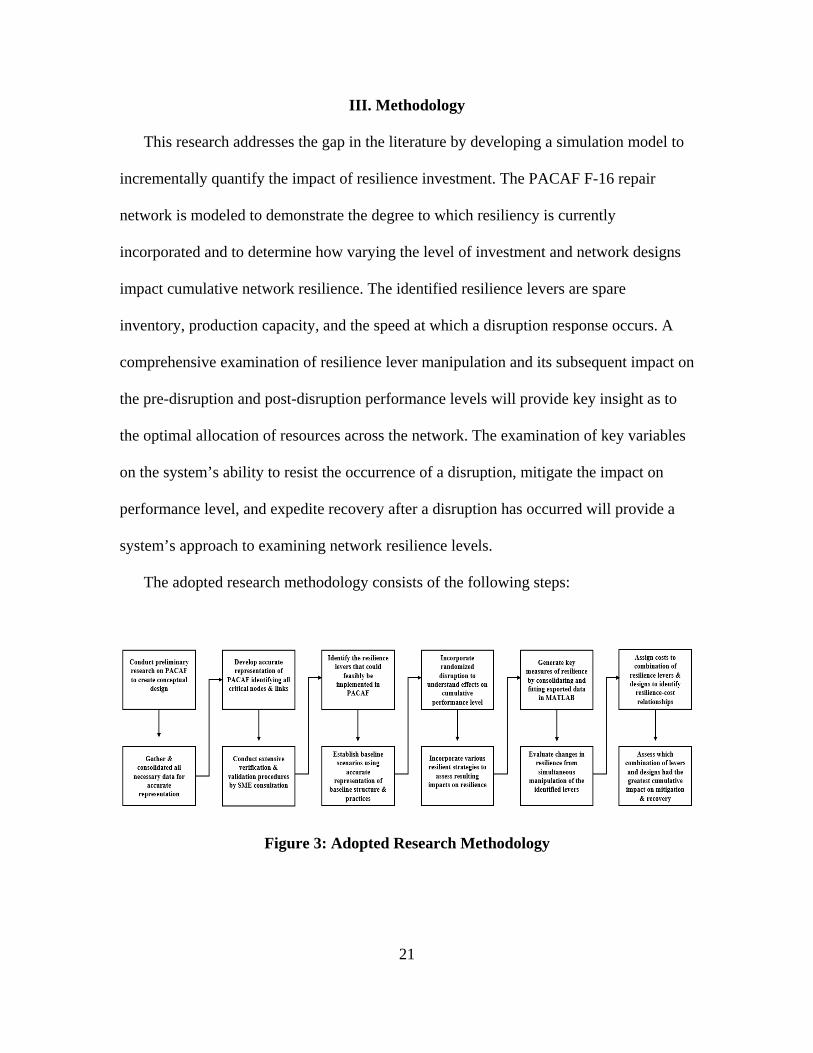
The adopted research methodology consists of the following steps:

Figure 3: Adopted Research Methodology

22

3.1 Conceptual Design

This research models the impact of a network disruption on the PACAF F-16 repair

network as it is currently structured. Furthermore, various network designs are proposed

and tested using the numerous flexibility approaches outlined in the literature. Repair

network operations located at Misawa AFB, Kunsan AFB, Osan AFB, and Eielson AFB

are modeled by incorporating four individual Product Repair Groups (PRGs): Propulsion,

Avionics, Hydraulics and Electrical & Environmental (E/E). The distribution of resources

(capital fixtures necessary for repair) for each location are based off the quantity of

resources for the F-16 C & D models located at Shaw AFB. For instance, identified

quantities of production capacity at Shaw AFB are distributed to each location in PACAF

in proportion to the amount of allocated aircraft located at each base. Table 1 illustrates

the back shop capacity allocation for the initial baseline system.

Table 1: Baseline System Capacity Allocation

3.2 Data Collection

The Air Force’s Logistics, Installations, and Mission Support-Enterprise View

(LIMS-EV) was utilized as the primary source of data. LIMS-EV is the “single entry

point” or consolidated warehouse of Air Force logistics data and was created to ensure

Back Shop Eielson Osan Kunsan Misawa TotalPropulsion 2 2 4 4 12Avionics 3 3 5 6 17

Hydraulics 1 2 3 3 9E/E 1 1 2 2 6

Prop CRF 5 5Total 7 8 14 20 49

23

“one version of the truth” for all logistics data exploitation (Petcoff, 2010). Therefore,

this research relies heavily upon the accessibility and accuracy of the consolidated

database. When identifying and gathering the necessary data, all results were filtered to

contain the relevant metrics for the chosen network and chosen airframe. Sortie quantity,

flying hours, total aircraft inventory (TAI), and break rates were gathered and

incorporated from various dashboards located within LIMS-EV. Furthermore, specific

line replaceable unit (LRU) data is gathered from the DLR Flying Dashboard.

Additionally, small focus groups with each PRG back shop were held that facilitated

discussion and validation of model assumptions. Conversations with subject matter

experts (SMEs) were utilized to gather pipeline times between critical nodes during the

repair process. Empirical data was gathered and consolidated from notes based on first-

hand experience at Shaw AFB. Table 2 shows a consolidated list of gathered and

incorporated data, while Table 3 illustrates the 2018 system parameters that are

incorporated into the simulation at time 0. Additionally, Custodian Inventory Reports

(R14s) were gathered from each PRG back shop located at Shaw AFB which contains the

item description, quantity on-hand, and original acquisition cost of all capital fixtures

necessary to perform repairs. The repair cycle time (RCT) was gathered for the

incorporated LRUs from SMEs located at the 635th Supply Chain Operations Wing

(SCOW).

24

Table 2: Consolidated Data Sources

Table 3: 2018 System Parameters

*Data changed in accordance to Distribution Statement A

3.3 Baseline System Description

This research utilizes SIMIO, a discrete-event simulation software well suited for the

design and emulation of complex, multi-layered problem sets requiring the use of many

experimental designs (Femano et al., 2019). To develop the most accurate representation

of the network, conversations with RNI Node Managers located at the SCOW were used

to validate repair capability assumptions for each modeled location. The validity of using

repair operations from Shaw AFB to model bases in PACAF was validated with SMEs.

The back shops in PACAF for the associated PRGs all have I-level capabilities except for

Data Data Source2018 Sortie Generation Data LIMS-EV: Weapon System View2018 PACAF Break Data LIMS-EV: Weapon System ViewPACAF Transportation Data USTRANSCOMPRG Categorization LIMS-EV: Cost of Logistics

NSN Demand DataLIMS-EV: Supply Chain Management View

NSN Cost Data D200: Dr. Marvin ArosteguiRepair Cycle Time (RCT) 635th SCOW: MSgt MarrCustodian Inventory Report (R14) PACAF SMEs

CAPEX EstimatesHistorical Air Force Construction Cost Handbook (2007)

Base AC* Sortie Quant* Total FH* Break Rate Sorties/Day* Hrs/Sort* DDay ProbEielson 25 2000 4000 13.82 7.69 2.00 0.25Osan 25 3000 5000 13.82 11.54 1.67 0.25

Kunsan 25 5000 8000 13.82 19.23 1.60 0.25Misawa 25 6000 9000 13.82 23.08 1.50 0.25

25

the propulsion capability. Operations are modeled by accurately duplicating the routing

of broken LRUs within each PRG. Each base contains flight line maintenance and the

respective back shop for each PRG. As broken LRUs are generated, the PRG that

contains the specific LRU is determined and used exclusively to route the part to the

appropriate back shop. Depending upon the severity, I-level breaks may be laterally

shipped to the base with the current capacity to perform the repair. I-level repairs may be

laterally shipped to the base that is most in need. Therefore, the network contains

organizational (O-level) and intermediate (I-level) capabilities. The only centralized

repair facility (CRF) is the propulsion back shop located at Misawa AFB. As breaks are

identified, and it is determined to be an engine, Eielson, Kunsan, and Osan all pack,

wrap, and ship whole engines to the Misawa propulsion CRF for repair. Therefore,

excluding propulsion, all local back shops possess I-level capabilities. Depot level

maintenance is not within the scope of this research.

Table 3 shows the quantity of assigned aircraft to each operating location in USAF’s

PACAF theater. Flying operations are conducted using 2018 flying schedule data. The

data is used to create an interarrival time of breaks as an exponentially distributed

function of the number of aircraft allocated to each base, the sortie quantity, flying hours,

and cumulative PACAF break rate. The interarrival time is given by:

𝐼𝐼𝐼𝐼𝐼𝐼𝐼𝐼𝐼𝐼𝐼𝐼𝐼𝐼𝐼𝐼𝐼𝐼𝐼𝐼𝐼𝐼𝐼𝐼 𝑇𝑇𝐼𝐼𝑇𝑇𝐼𝐼 = (𝐹𝐹𝑖𝑖

𝐵𝐵𝐼𝐼𝐼𝐼𝐼𝐼𝐵𝐵𝐵𝐵𝐼𝐼𝐼𝐼𝐼𝐼)/(𝐴𝐴𝑖𝑖 ∗ 𝑆𝑆𝑖𝑖 ∗ 𝐻𝐻𝑖𝑖) (1)

where,

𝑭𝑭𝒊𝒊 represents the total flying hours for base i,

26

𝑨𝑨𝒊𝒊 is the total number of mission capable aircraft at any given time for base i,

𝑺𝑺𝒊𝒊 is the average number of sorties using a 260-day flying schedule for base i,

𝑯𝑯𝒊𝒊 is the average duration in hours of each sortie for base i.

As an entity is generated (break occurs), an LRU is assigned, which corresponds to a

PRG, thereby determining the routing of the part in the repair process. LRU assignment is

based upon the 2018 annual demand for each LRU determined in LIMS-EV.

As the discrepancy is identified by flight line maintenance, crews will determine the

PRG and ultimately the LRU that has failed. As Table 4 and Table 5 illustrate, a severity

of 1 to 4 is assigned to all breaks for propulsion, avionics, E/E, and hydraulics. The

propulsion severity mix is drawn from a separate table to enable this research to more

accurately reflect the number of propulsion I-level discrepancies. As the LRU arrives at

the appropriate back shop, the associated repair cycle time is determined and assigned as

a random exponential distribution. The repair cycle time was assigned to each LRU by

using a weighted average based off the corresponding annual demand for each LRU.

However, if an engine was routed to the propulsion CRF, a processing time of 30-days is

used to represent an accurate depiction of the amount of time to turn the engine

serviceable. The weighted average was necessary to realize the benefits from incremental

investment in production capacity. The weighted average raised the repair time for higher

demanded items, thus allowing a queue to build at the associated back shops. The

baseline structure features one propulsion CRF. If a propulsion LRU is generated, and

severity 4 is assigned, the entire engine is dropped and routed to the CRF located at

Misawa. For propulsion, avionics, E/E, and hydraulics, severities 1 to 3 are routed

27

directly to the local back shop. Excluding propulsion, lateral shipments of severity 4

breaks are permitted which provides the flexibility to ship the part to the base which

currently has the available capacity to perform the repair. As the part is repaired at the

back shop, the repaired part will be shipped to the base that is currently most in need,

where the part will be placed on an awaiting aircraft or increase local on-hand spare

inventory as depicted in Figure 5.

Table 4: Avionics, Hydraulics, & E/E Severity Mix

Table 5: Propulsion Severity Mix

3.4 Model Verification & Validation

Extensive model verification occurred using the model trace function in SIMIO.

Tracing allows the step-by-step tracking of individual entities flowing from node to node

throughout the duration of the repair process. A method was followed that verified the

precise location of each entity within the simulation. This verification ensured the proper

assignment of specific PRGs and subsequently, LRUs, which led to the verification of

routing to the appropriate back shop and/or CRF. Model assumption validation was

Eng Sev Sev Mix Rpr Lvl BSProcessingTime (Hrs) Prop CRF (Days)1 0.45 O-Level LRU RCT -2 0.13 O-Level LRU RCT -3 0.17 O-Level LRU RCT -4 0.25 I-Level LRU RCT -

Eng Sev Sev Mix Rpr Lvl BSProcessingTime (Hrs) Prop CRF (Days)1 0.35 O-Level LRU RCT -2 0.25 O-Level LRU RCT -3 0.2 O-Level LRU RCT -4 0.2 I-Level - Random.Exponential (30)

28

achieved based on continuous feedback from conversations with SMEs located at Shaw

AFB, the 635th SCOW, and PACAF. Time series outputs of total throughput, processing

times, and queues were generated to validate system performance over time.

Each iteration completion generated system statistics that provided metrics such as

the number of breaks specific to each location, number of repairs specific to each

location, and system utilization metrics such as throughput and time in system.

Utilization metrics were validated with phone calls to SMEs located at the specific back

shops in PACAF.

3.5 Scenario Development

Baseline scenarios were first developed to aid in the verification and validation

process and to gain a fundamental understanding of the system’s performance levels.

Baseline scenarios were generated with current PACAF repair capabilities to provide an

accurate representation of system behavior over time. All scenarios were run over a

2,000-day time period with an incorporated warm-up period of 1200-days. Due to the

size and inherent complexities of the model, a 1200-day warm-up period was necessary.

Although system statistics are generated for an 800-day time period, this research

primarily focuses on the transient states of performance. For instance, a randomized

disruption occurs at day 1400. Regardless of the response time frame, all scenarios have

recovered by day 1600. Therefore, from day 1400 to 1600, the AUC is utilized to

evaluate system performance. The baseline structure represents the PACAF F-16 repair

network as it is currently structured. Therefore, all other resilience scenarios and network

29

designs will be compared to the baseline structure in both performance and cost over the

specified time period.

This research uses the following classifiers to identify the time periods of interest

during a disruption:

Pre-Disruption: Day 1200 to day 1400

Post Disruption – Decline: The time at which the disruption occurs until a specified

response has been enacted.

Post Disruption – Recovery: Time at which the response occurs until the system

performance has recovered (Day 1600).

Existing within the post disruption time period is the AUC metric used to quantify the

level of demand the network can meet during the Post Disruption - Decline and Recovery

periods. The AUC for each period is described as follows (Femano et al., 2019):

Area under the Curve – Decline (AUC-Decline): The total network performance under

the Post Disruption – Decline curve.

Area under the Curve – Recovery (AUC – Recovery): The total network performance

under the Post Disruption – Recovery curve.

Area under the Curve – Total (AUC – Total): Cumulative network performance during

all stages of the disruption.

The primary resilience levers are production capacity and response time. However,

the simultaneous investment in spare inventory is essential to realize the greatest benefit

from increased capacity (Femano et al., 2019). All expanding scenarios include some

allocation of inventory, production capacity, and a varying response time. Table 6

30

illustrates the developed scenarios used for the baseline structure. A cost and

performance threshold of 80% MC Rate was used to scope the number of needed

scenarios. Baseline structure capacity is varied up to a 30% increase of the originally

assigned allocations, while the capacity used to recover from the disruption is increased

up to 50% of the initial capacity allocation. Additionally, the scenarios in Table 6 were

used in conjunction with a 10, 20, 30, and 40-day response time to emphasize the

importance of an expedited response. All designed scenarios were evaluated using the

developed AUC metric, in addition to the network’s cumulative mission capable (MC)

rate. Moreover, 100 replications were performed on each scenario. The AUC is used as

the primary metric of resilience because it provides a more accurate representation of

system behavior and the ability to meet demand over the disrupted time period.

Table 6: Developed Baseline Scenarios

ScenarioSystem Initial

Capacity

Recovery Capacity Scenario

System Initial

Capacity

Recovery Capacity

1 1.00 13 1.002 1.10 14 1.103 1.20 15 1.204 1.30 16 1.305 1.40 17 1.406 1.50 18 1.507 1.00 19 1.008 1.10 20 1.109 1.20 21 1.2010 1.30 22 1.3011 1.40 23 1.4012 1.50 24 1.50

Initial System

1.00 1.20

1.10 1.30

31

As replications are completed, SIMIO produces and exports a comma separated value

(CSV) file for each replication. The baseline scenarios outlined by Table 6 produced

2,400 CSVs for one response time (100 files for each scenario). After all developed

scenarios have been completed, the CSVs are imported into MATLAB, which

consolidates, batches, and integrates the area under the curve for each scenario.

MATLAB then produces a consolidated table containing the time period metrics

associated with each scenario that are used for investment and design comparison. All

consolidation, batching, and integration code can be seen in detail in appendix B, C, and

D.

3.6 Flexibility Design

In addition to varying amounts of predetermined resilience levers, network design

performance is evaluated using the process flexibility approach introduced by Jordan and

Graves (1995) and Simchi-Levi and Wei (2012) in the literature. The process flexibility

approach assumes a finite amount of network production capacity and varying amounts

of connectedness among repair nodes. For instance, the baseline structure is rather robust,

and all locations have avionics, hydraulics, and E/E capabilities. For propulsion,

however, centralization exists for I-level capabilities. Hence, the baseline system

provides adequate resistance to disruptions that are enacted upon it. However, if the CRF

at Misawa for propulsion is affected, the subsequent events that follow and the impact on

the network’s ability to perform engine overhauls would be disastrous. Therefore, various

levels of flexibility were implemented and tested using allocations of network resources

to do so.

32

This research employs two additional designs selected for their stark cost/resilience

difference when facing uncertain futures. Each location is assigned the initial amount of

production capacity in proportion to the amount of allocated aircraft as presented in Table

1. The employed network designs strategically increment capacity at various locations to

illustrate the impact on the network’s ability to maintain system throughput at the back

shops in the event of lost capacity at a location. Figure 4 illustrates the differences

between the various network designs.

Figure 4: Developed Network Designs

The second design uses the long chain flexibility approach developed by Jordan and

Graves (1995). This approach is extremely beneficial for system designs that feature

limited flexibility incorporation. However, as the baseline structure is rather flexible

regarding the allocation of repair capabilities, it is not flexible when capacity is

33

considered. This research employs the long chain approach to illustrate an alternative

design to achieve desired levels of flexibility at tremendous cost savings. The inability to

alter PACAF as it is currently structured is recognized. Therefore, we posit the use of the

long chain strategy to recommend methods of future capacity expansion. As Jordan and

Graves (1995) describe, the capacity for each PRG is allocated to exactly two locations.

Every location possesses the ability to perform repairs for exactly two PRGs, which

forms “one chain” flexibility as illustrated in Figure 2 and disperses cumulative risk

(Jordan & Graves, 1995). The third design, or simple allocation structure, supplements all

existing recovery capacity at non-impacted locations with Misawa’s production capacity

(greatest quantity). Chosen to illustrate the impacts of significantly increasing recovery

capacity on the AUC, this design illustrates the cost associated with a higher level of

resilience. Additionally, the simple allocation structure realizes a large increase in spare

inventory across all locations to illustrate the need for simultaneous investment to support

the increase in production capacity. Furthermore, multiple propulsion CRFs are utilized

to show the benefits of centralization dispersion. All developed designs are evaluated

using the experimentation function in SIMIO to allow the simultaneous manipulation of

the identified resilience levers. Additionally, all established designs possess the ability to

laterally ship I-level discrepancies.

The long chain structure increases levels of recovery capacity only. The simple

allocation structure does not realize an additional investment in initial or recovery

capacity due to the extremely large initial resilience investment. Furthermore, the long

chain structure increases up to 210% of the original long chain initial capacity allocation.

The large investment increase in the long chain scenarios was cost feasible and necessary

34

to reach Pre-Disruption MC Rates. Similar to the simple allocation structure, the long

chain structure’s large increase in recovery capacity warranted an increase in spare

inventory for the design.

3.7 Disruption Incorporation

All developed scenarios were run using predetermined resilience levers over 2,000-

days to gain a fundamental understanding of the impacts of simultaneously manipulating

resilience levers on cumulative system performance. To gauge system performance and

to determine the level of system resilience, all developed scenarios were run with the

incorporation of a randomized disruption (DDay) at day 1400, where, as Table 3

illustrates, a disruption eliminates all the repair capabilities specific to one location via an

equal probability. After a specified delay, it is assumed all aircraft that were located at the

impacted location are equally distributed to the three remaining bases. Moreover, this

research assumes that operations at the impacted location are unrecoverable and

therefore, lost for the remaining duration of the simulation. Furthermore, process logic

prevents all subsequent I-level breaks from being routed to the impacted location. Figure

5 illustrates the general pre- and post-disruption behavior.

35

Figure 5: Post-Disruption Behavior

3.8 Resilience Measurement

Consistent with Melnyk et al. (2013), this research argues that system resilience is

most accurately assessed during the system’s transient states. Shown in Figure 6, each

simulation iteration was broken into three distinct time periods as described in section 3.5

(Femano et al., 2019). This research builds upon the foundation set forth in the literature

by using the identified concepts to illustrate and quantify the effects of simultaneous

manipulation of resilience levers on each of the three time periods. As Figure 6

illustrates, the system’s resistance to the disruptive event occurs in the Pre-Disruption

time period of the simulation. The recovery of the system begins at the Minimum

Performance Level (MPL) of the system during the disruptive event and ends in the Post

Disruption – Recovery time period.

36

Figure 6: Performance Metrics & Disruption Time Periods (Femano et al., 2019)

This research employs the concept of the AUC to quantify the number of MC days

that the system can support resulting from various levels of resilience investment

(Femano et al., 2019). Contrary to Melnyk et al. (2013), who employ the use of the area

above the disruption curve, this research argues that the AUC provides a more accurate

representation of cumulative performance over the disruption time period. The area above

the curve measures lost performance in the event of a disruption, which ultimately,

deemphasizes network starting performance (Femano et al., 2019). Additionally, this

research further develops a generalizable resilience metric, which represents the networks

achieved AUC in proportion to the desired AUC, or total realized demand over the

disruption time period (Femano et al., 2019).

𝐵𝐵𝐼𝐼𝑅𝑅𝐼𝐼𝐼𝐼𝐼𝐼𝐼𝐼𝐼𝐼𝑅𝑅𝐼𝐼 𝑀𝑀𝐼𝐼𝐼𝐼𝐼𝐼𝐼𝐼𝑅𝑅 = 𝐴𝐴𝐴𝐴𝐴𝐴𝑡𝑡𝐷𝐷𝑡𝑡

(2)

37

This metric proves extremely generalizable because regardless of the organization, it will

experience some drop in performance resulting from a disruption, and it will experience

some level of demand that must be met during the disruption. Hence, this resilience

metric provides an indication of the level of demand that can be met due to various levels

of resilience investment. The analysis and results section builds upon the associated time

periods and AUC by introducing the various time period metrics illustrated in Figure 6.

3.9 Cost Assignment

Essential to the foundation of this research is the ability to monetarily quantify

varying levels of investment. Cost estimates of the associated capacity and inventory

allocations, as well as the capital expenditures necessary to house them, allows decision

makers to associate the required level of investment needed to reach a desired level of

resilience. This research employs USAF R14s to assign a cost to the ability to perform a

simultaneous repair at each specific back shop. For example, the propulsion R14 for

Shaw AFB was used as the basis of cost for one unit of incremental capacity across all

propulsion locations in the developed scenarios. Cost was linearly assigned to provide a

representation of the necessary investment.

Spare inventory quantities were gathered specific to each location using the D200

database. Furthermore, the cost of each LRU was gathered from D200 and linearly

assigned to each incremental unit of spare inventory.

An accurate representation of the necessary capital expenditures is essential for

illustrating the benefits of the long chain strategy. Hence, generalizable costs associated

with the CAPEX repair facilities were gathered using the Historical Air Force

38

Construction Cost Handbook (2007). Costs were determined using the given size (square

feet) and cost per square foot. Additionally, location specific factors, which account for

the specific costs of construction associated with each modeled location, were used in

generating a final cost estimate.

Lastly, the cost of personnel needed at each location was determined by taking the

average annual base pay of personnel with the pay grade of E-1 to E-7 with 2 through 20

years in service to generate an average annual salary. This figure was multiplied by the

number of individuals located at each repair back shop across all locations. This research

recognizes that as the level of production capacity increases, so too does need for

personnel. Hence, the cost of personnel is increased by the cost percentage increase in

production capacity as compared to the initial production capacity investment for each

design.

An important distinction must be made regarding cost assignment. All incorporated

costs represent the fixed costs necessary to perform a repair. Personnel, however, border

the line between fixed and operational costs. Personnel costs are included for the purpose

of this research because personnel are a fixed requirement for a given repair capability

over the time periods for which the model is run.

39

IV. Analysis and Results

This research tests three network designs: baseline structure, simple allocation

structure, and the long chain structure. PACAF was strategically chosen as the test case to

apply this simulation because of the rising capabilities of US adversaries and

vulnerabilities of the network to natural disaster. The simple allocation and the long chain

structure reiterates the need for simultaneous investment in inventory and production

capacity, while also illustrating the realized benefits and cost differences in various levels

of flexibility incorporation. All scenarios used to test the various network designs are

evaluated during their transient states. Numerous disruption response times are

implemented that “turn on” predetermined amounts of recovery capacity for the specific

scenario. Hence, this research shows the importance of predetermined asset allocations

on a location’s ability to respond to a disruption. An important distinction will be made

regarding the costs of these production capacity assets in the resilience cost section.

Associated with the established time periods outlined in section 3.5 are three

performance metrics: The Pre-Disruption MC Rate, the Minimum Performance Level

(MPL), and the Recovery Performance Level (RPL). Fully understanding the

performance of a network in the event of a disruption requires a deep understanding of

the interconnectedness of the mentioned performance metrics. They are defined as

follows:

Pre-Disruption MC Rate: The average daily MC Rate from day 1200 to day 1400.

Minimum Performance Level (MPL): The network’s minimum level of performance

resulting from a disruption.

40

Recovery Performance Level (RPL): The average daily performance after network

performance has recovered.

The following sections illustrate the importance of these metrics on network

performance. The emphasis is on the ability to maintain performance after the disruption

has occurred. In doing so, the ability to meet a specified level of demand during a

disruption begins where the Pre-Disruption MC Rate ends. In other words, a network’s

starting performance is extremely important for cumulative system performance

throughout all stages of a disruption.

4.1 Baseline Structure

The baseline structure represents PACAF as it currently operates. It provides valuable

insight as to how the network resists and recovers from a disruption due to its inherent

flexibility and current capabilities. Table 7 shows the output generated from the

developed scenarios outlined in Table 6. Each scenario represents a predetermined level

of initial capacity and recovery capacity. The scenario with 1.00 of initial and recovery

capacity represents PACAF’s performance without any additional investment in

resilience. No additional investment in production capacity leads to grave consequences.

For instance, all bases have an equal probability of experiencing a disruption. If Misawa

experiences the disruption, the CRF and all other repair capabilities are lost, further

exacerbating the consequences on PACAF cumulative performance.

4.1.1 Impacts on Transient Performance Metrics

The baseline structure does not simultaneously increase the investment in spare

inventory as the amount of capacity increases. However, Table 7 emphasizes the

41

importance in a network’s ability to maximize its Pre-Disruption MC Rate in the event of

a disruption. The transient performance of the network starts with the Pre-Disruption MC

Rate, and the higher the starting point for the decline to occur, the greater the AUC -

Decline will be. Shown in Table 7, as the investment in initial capacity increases, so too

does the Pre-Disruption MC Rate, yielding a higher AUC – Decline and MPL.

Subsequently, a higher MPL leads to the ability to meet a greater level of demand during

the Post Disruption – Recovery period as illustrated by the increase in AUC – Recovery

and ultimately a higher RPL. Similarly, Figure 7 illustrates the impact of an expedited

response time and additional production capacity investment on the network’s AUC –

Total. However, an important phenomenon is illustrated in the baseline structure. Notice

that the RPL realizes marginal gains as the Pre-Disruption MC Rate increases. This

further reiterates the necessity of simultaneous investment in inventory and production

capacity. Although the network’s ability to perform in the face of disruption undoubtedly

increases with a greater level of investment, a sub-optimal output is realized when only

production capacity is increased. This point is further illustrated using the simple

allocation and long chain structure. Alternatively, the investment in recovery capacity has

the greatest benefit to RPL in the baseline structure.

42

Table 7: Baseline 40-Day Response Output

Pre Disruption

Initial Cap Recovery Cap Avg MC Rate MPL AUC-D RPL AUC-R AUC-Total Total $$

1.00 70.74 53.04 11,261 N/A N/A 11,261 126,246,142$

1.10 70.74 58.06 2,560 58.84 9,481 12,041 127,402,468$

1.20 70.74 58.09 2,560 61.83 9,870 12,430 128,405,856$

1.30 70.74 58.09 2,560 65.85 10,463 13,023 129,233,582$

1.40 70.74 58.09 2,560 71.82 11,355 13,915 130,546,799$

1.50 70.74 58.09 2,560 74.75 11,815 14,374 131,319,197$

1.00 75.08 54.61 2,686 54.51 9,157 11,842 127,402,468$

1.10 75.08 57.10 2,686 55.56 9,437 12,123 128,558,794$

1.20 75.08 59.01 2,686 58.36 9,770 12,456 129,562,182$

1.30 75.08 59.88 2,686 63.34 10,391 13,077 130,389,908$

1.40 75.08 59.95 2,686 71.03 11,261 13,947 131,703,125$

1.50 75.08 59.95 2,686 74.33 11,739 14,425 132,475,523$

1.00 77.71 60.35 2,844 59.13 9,820 12,663 129,992,628$

1.10 77.71 62.54 2,844 60.27 10,099 12,943 131,148,954$

1.20 77.71 64.22 2,844 62.17 10,358 13,202 132,152,342$

1.30 77.71 64.61 2,844 66.90 11,012 13,855 132,980,068$

1.40 77.71 64.66 2,844 73.57 11,697 14,540 134,293,285$

1.50 77.71 64.69 2,844 77.03 12,167 15,011 135,065,683$

1.00 82.86 63.80 3,030 63.20 10,512 13,542 130,820,354$

1.10 82.86 65.90 3,030 64.52 10,973 14,003 131,976,679$

1.20 82.86 67.59 3,030 66.48 11,125 14,155 132,980,068$

1.30 82.86 69.46 3,030 67.84 11,388 14,419 133,807,793$

1.40 82.86 69.46 3,030 72.36 12,239 15,269 135,121,011$

1.50 82.86 69.46 3,030 75.42 12,389 15,419 135,893,408$

Scenario Post-Disruption - Decline Post Disruption - Recovery

1.00

1.10

1.20

1.30

43

Figure 7: Baseline Response Comparison (10 vs. 40-Day)

4.1.2 Criticality of Response Time

An organization’s ability to quickly identify and respond to a disruption is essential to

its performance during and after a disruption. The disruption response time is varied after

a disruption occurs and assumes that the response time is tied directly to the ability to

“turn on” the predetermined asset allocations of recovery capacity at the remaining

locations. The response time is a function of an organization’s ability and willingness to

invest in predetermined asset allocations. Figure 8, Figure 9, and Table 8 illustrate the

consequences of a prolonged response time on cumulative network performance.

44

Figure 8: Varying Response Time - Baseline Structure (1.00 Initial Cap, 1.40

Recovery Cap)

Figure 9: All Responses – Baseline Structure (1.00 Initial Cap, 1.40 Recovery Cap)

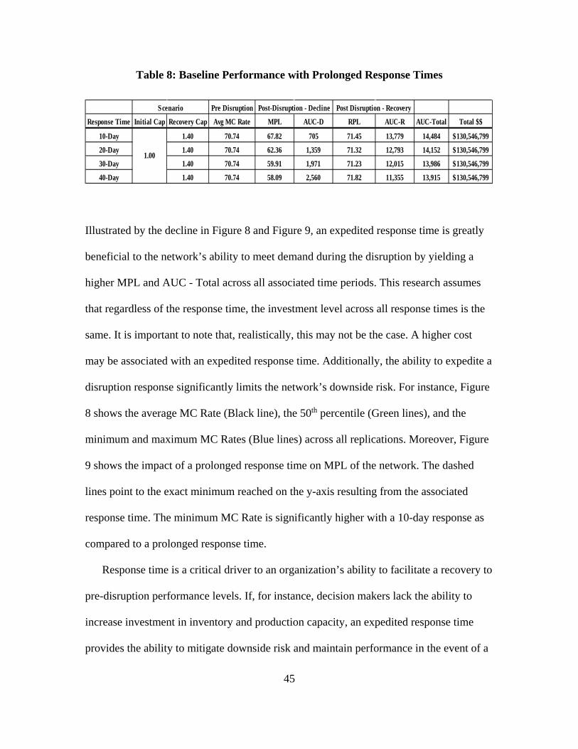
45

Table 8: Baseline Performance with Prolonged Response Times

Illustrated by the decline in Figure 8 and Figure 9, an expedited response time is greatly

beneficial to the network’s ability to meet demand during the disruption by yielding a

higher MPL and AUC - Total across all associated time periods. This research assumes

that regardless of the response time, the investment level across all response times is the

same. It is important to note that, realistically, this may not be the case. A higher cost

may be associated with an expedited response time. Additionally, the ability to expedite a

disruption response significantly limits the network’s downside risk. For instance, Figure

8 shows the average MC Rate (Black line), the 50th percentile (Green lines), and the

minimum and maximum MC Rates (Blue lines) across all replications. Moreover, Figure

9 shows the impact of a prolonged response time on MPL of the network. The dashed

lines point to the exact minimum reached on the y-axis resulting from the associated

response time. The minimum MC Rate is significantly higher with a 10-day response as

compared to a prolonged response time.

Response time is a critical driver to an organization’s ability to facilitate a recovery to

pre-disruption performance levels. If, for instance, decision makers lack the ability to

increase investment in inventory and production capacity, an expedited response time

provides the ability to mitigate downside risk and maintain performance in the event of a

Pre Disruption

Response Time Initial Cap Recovery Cap Avg MC Rate MPL AUC-D RPL AUC-R AUC-Total Total $$

10-Day 1.40 70.74 67.82 705 71.45 13,779 14,484 130,546,799$

20-Day 1.40 70.74 62.36 1,359 71.32 12,793 14,152 130,546,799$

30-Day 1.40 70.74 59.91 1,971 71.23 12,015 13,986 130,546,799$

40-Day 1.40 70.74 58.09 2,560 71.82 11,355 13,915 130,546,799$


1.00

46

disruption. Therefore, an expedited response time is a viable alternative to hedge against

the inability to use resources that have been lost in the event of a disruption.

4.2 Simple Allocation Structure

The simple allocation structure realizes a significant increase in resilience investment

across all locations. The simple allocation structure allocates the network’s greatest

capacity quantity (Misawa) and assigns it as recovery capacity at all other locations.

Furthermore, the simple allocation structure incorporated an additional propulsion CRF at

Kunsan to illustrate the beneficial impacts of decentralization on network performance

while facing disruptions. Additionally, and in a similar manner to production capacity,

the simple allocation structure allocated Misawa’s spare inventory quantity across all

locations to illustrate the need for simultaneous inventory investment to realize the

greatest benefit from the increase in recovery capacity. Therefore, the simple allocation

structure demonstrated the highest level of resilience resulting from the large increase in

resilience investment. Table 9 highlights the performance and costs of the simple

allocation structure. Due to the large increase in resilience and subsequent performance,

an increased investment in initial and recovery capacity was not utilized. Hence, the

number of needed scenarios was drastically reduced.

Table 9: Simple Allocation Structure Output

Pre Disruption


10-Day 1.00 72.66 68.82 727 84.84 16,783 17,510 177,264,060$

20-Day 1.00 72.66 61.00 1,453 85.42 15,263 16,716 177,264,060$

30-Day 1.00 72.66 55.39 2,180 85.57 14,418 16,598 177,264,060$

40-Day 1.00 72.66 53.91 2,858 86.17 13,632 16,490 177,264,060$

1.00


47


Table 9 illustrates the impact of higher initial inventory quantities on the network’s

Pre-Disruption MC Rate. Spare inventory has a greater impact on the ability of the

system to resist the occurrence of a disruption (Melnyk et al., 2013). As shown, the Pre-

Disruption MC Rate is greater in the simple allocation structure than in the baseline

structure at the same level of initial capacity investment. Thus, the simple allocation

structure leads to a higher MPL across all scenarios and response times at the same level

of initial capacity as compared to the baseline structure. Furthermore, due to the high

level of investment in recovery capacity, the corresponding RPL and AUC – Recovery all

meet significantly higher demand. Thus, recovery capacity has the greatest impact on a

network’s ability to recover from a disruption.


The ability of an organization to expedite its disruption response is further

emphasized using the simple allocation structure design. Regardless of the investment in

recovery capacity, decision makers must emphasize the need of a rapid response to

realize the full potential of the recovery capacity.

4.3 Long Chain Structure

The third design uses the long chain flexibility approach identified in the literature to

allocate production capacity across PACAF (Jordan & Graves, 1995). Note that the

baseline structure is inherently flexible. For instance, each location possesses I-level

repair capabilities for at least three PRGs. The exception is Misawa due to its ability to

perform the repair of propulsion I-level discrepancies. Therefore, the long chain approach

48

eliminates a portion of the inherent flexibility of the network by allocating the ability to

perform the repair of only two PRGs at each location. In doing so, the original production

capacity allocation for each PRG is split and assigned to the two locations that possess

capabilities for that specific PRG in equal sums. The initial capacity quantity for the

network is equal to that of the baseline structure. Furthermore, only recovery capacity is

increased in the developed scenarios. Due to the large investment necessary in recovery

capacity to recover to pre-disruption performance levels, the developed long chain

scenarios were duplicated, once with no added spare inventory, and once with an

additional investment in spare inventory. The results are compared in Table 10 and Table

11, which also show the developed scenarios and response output for the 10-day response

time. Figure 10 shows the impact of additional resilience investment and an expedited

response time on the network’s AUC – Total.

49

Table 10: Long Chain 10-Day Response Output Original Inventory Levels

Table 11: Long Chain 10-Day Response Output Increased Inventory Levels

Pre-Disruption


1.00 68.19 46.92 10,412 N/A N/A 10,412 93,286,471$

1.10 68.19 44.34 680 44.34 9,954 10,634 94,465,440$

1.20 68.19 48.58 680 48.58 10,354 11,034 95,775,334$

1.30 68.19 51.14 680 51.14 10,562 11,243 97,337,275$

1.40 68.19 53.71 680 53.71 10,921 11,602 98,559,419$

1.50 68.19 57.21 680 57.21 11,427 12,107 99,938,087$

1.60 68.19 58.44 680 58.44 11,588 12,269 101,005,107$

1.70 68.19 60.22 680 60.22 11,864 12,544 102,227,250$

1.80 68.19 63.04 680 63.04 12,174 12,854 103,789,191$

1.90 68.19 64.75 680 64.75 12,500 13,180 105,099,086$

2.00 68.19 65.19 680 65.19 12,667 13,347 106,278,054$

2.10 68.19 66.03 680 66.03 12,973 13,653 107,457,023$

Scenario Post Disruption - Decline Post Disruption - Recovery

10-Day 1.00

Pre-Disruption


1.00 71.14 51.37 11,121 N/A N/A 11,121 96,038,078$

1.10 71.14 52.51 711 52.68 10,602 11,313 97,217,046$

1.20 71.14 55.69 711 55.33 11,151 11,863 98,526,941$

1.30 71.14 57.04 711 57.07 11,465 12,176 100,088,882$

1.40 71.14 58.10 711 58.90 11,640 12,351 101,311,025$

1.50 71.14 60.11 711 60.99 11,996 12,707 102,689,694$

1.60 71.14 61.61 711 62.52 12,199 12,910 103,756,713$

1.70 71.14 62.73 711 63.85 12,410 13,121 104,978,857$

1.80 71.14 64.68 711 65.36 12,684 13,396 106,540,798$

1.90 71.14 66.88 711 67.67 13,069 13,780 107,850,692$

2.00 71.14 68.48 711 68.81 13,327 14,039 109,029,661$

2.10 71.14 68.61 711 69.90 13,476 14,188 110,208,629$

Scenario Post Disruption - Decline Post Disruption - Recovery

10-Day 1.00

50

Figure 10: Long Chain Response Comparison (10 vs. 40-Day)


Perhaps there is no better example of the need for simultaneous investment than the

developed long chain scenarios. Although the realized benefits of increased investment

on disruption performance is consistent with the previous designs, the impacts of

increased inventory on the network’s ability to maintain a higher level of demand are

undeniable. Mentioned throughout this research is the need to invest in inventory and

production capacity in unison. To invest in one without the other will lead to a sub-

optimal output (Femano et al., 2019). Table 11 greatly reiterates this point. Within all

stages of the disruption, the scenarios with an increased investment in inventory

outperformed the scenarios that did not simultaneously increase the investment. For

instance, higher quantities of inventory facilitated a higher Pre-Disruption MC Rate,

which led to a higher MPL across all scenarios. Furthermore, and contrary to the baseline

51

scenarios which experienced a higher starting point due to the increased investment in

initial capacity, the greater starting point facilitated a greater RPL for the scenarios with

increased inventory. Once again, this is due to the need for an increase in inventory to

realize the greatest potential from the increase in production capacity.


Due to the inherent structure of the long chain design, the total production capacity

for one PRG is halved and allocated to each assigned location. When a disruption occurs,

the network loses a greater portion of the allocated production capacity as compared to

the baseline or simple structure. Hence, the impact of a disruption without an appropriate

predetermined asset allocation is further exacerbated. As shown in the following section,

the benefits from employing the long chain approach comes from the ability to invest in a

greater amount of capacity to respond to a disruption at a much lesser cost. This

production capacity allocation inherently places a greater need to respond after a

disruption has occurred. Figure 11 and Figure 12 show the beneficial impacts of an

expedited recovery using the long chain approach. Similar to Figure 8, Figure 11

provides the average MC Rate (Black line), the 50th percentile (Green lines), and the

minimum and maximum MC Rates (Blue lines) across all replications.

52

Figure 11: Varying Response Time – Long Chain Structure (1.00 Initial Cap, 2.10

Recovery Cap)

Figure 12: All Responses – Long Chain Structure (1.00 Initial Cap, 2.10 Recovery

Cap)

53

Table 12: Long Chain Performance with Prolonged Response Times

As outlined in the literature, if an organization’s ability to respond to a disruption is

obstructed, the use of increased inventory creates a resistance to the disruption by

enabling the organization to maintain a higher level of performance after the disruption

occurs (Melnyk et al., 2013; Femano et al., 2019). Table 11 shows that the greater

quantity of inventory provides a greater AUC – Decline and AUC – Recovery. Therefore,

if an expedited response time is not feasible, greater levels of inventory provide the

ability to hedge against downside risk by providing resistance to the disruption.

4.4 Resilience Costs

The PACAF theater is used to demonstrate the applicability of the developed tool, but

this research provides a generalizable simulation tool that may be applied across multiple

domains. The assigned costs are specific to that of PACAF, but the structure of this tool

allows ease of translatability across numerous theaters, airframes, and industry related

repair networks.

From a cost feasibility standpoint, this research recognizes that the simple allocation

structure is not likely to be implemented. It is included to further emphasize the

importance of decentralization and simultaneous investment. The long chain structure

inherently subtracts from the flexibility of the baseline and simple allocation structure.

Pre Disruption


10-Day 2.10 71.14 68.61 711 69.90 13,476 14,188 110,208,629$

20-Day 2.10 71.14 63.93 1,385 70.18 12,524 13,909 110,208,629$

30-Day 2.10 71.14 59.40 2,004 69.93 11,730 13,734 110,208,629$

40-Day 2.10 71.14 57.73 2,587 70.06 10,989 13,576 110,208,629$

1.00


54

However, the cumulative performance of the overall network is extremely comparable to

that of the baseline structure at a substantially reduced cost. When implementing the long

chain design, the massive cost savings are realized from the decrease in the large capital

expenditures necessary to house the repair capabilities of four PRGs at one location.

Figure 13 illustrates the usefulness of the resilience metric when comparing

performance across multiple structures and response times. Specifically, Figure 13

provides insight into the level of resilience investment needed to reach Pre-Disruption

MC Rates (1.00) after a disruption occurs using the baseline and long chain structures.

More importantly, Figure 13 highlights the overlapping performance and stark cost

difference between the baseline and long chain structures.

The resilience metric provides a direct indication of how an organization performs in

the event of a disruption. When a disruption strikes, demand does not cease to exist.

Therefore, regardless of the organization, some level of demand will need to be met when

a disruption occurs. The resilience metric allows decision makers and organizations to

predict the level of demand that can be met resulting from predetermined investments in

resilience.

55

Figure 13: Structure Performance/Cost Comparison

4.5 Validity of an Expedited Response Time

Figure 13 combines the scatter output from the baseline and long chain structures for

performance and cost comparison. As the investment in resilience increases using the

long chain structure, the resulting AUC – Total increases linearly. Additionally, the

difference between the 10- and 40-day response time is clear. However, as the resilience

investment is increased using the baseline structure, the results are not as distinct between

the 10- and 40-day response. To validate that there is in fact a difference between an

expedited and a prolonged response time in AUC - Total, this research employed the

Paired T-Test to statistically test the difference between varying responses. A Paired T

Test was chosen to test the difference between the two dependent samples (Milton &

Arnold, 2003). Specifically, this test allows the researcher to evaluate the following:

56

𝐻𝐻0:𝑢𝑢𝑥𝑥 = 𝑢𝑢𝑦𝑦 𝐻𝐻1:𝑢𝑢𝑥𝑥 > 𝑢𝑢𝑦𝑦

(3)

which determines whether there is a statistical difference between the response time

means. To conduct the statistical test, a test statistic was developed from the following

equation (Milton & Arnold, 2003):

𝑇𝑇 𝑆𝑆𝐼𝐼𝐼𝐼𝐼𝐼 = 𝑢𝑢𝐷𝐷 − 0𝑆𝑆𝐷𝐷/√𝐼𝐼

(4)

where,

uD is the mean of the differences between two response times,

0 is the hypothesized difference between two response times,

SD is the standard deviation of the difference in means between two response times,

n is the sample size.

Since multiple response times are being analyzed, the chance of rejecting the null

hypothesis when it is true (type 1 error), drastically increases (Statistics Solutions, 2019).

Hence, the Bonferroni correction was implemented to lower the significance level by

dividing 0.05 by 4 (the number of response time comparisons) (Statistics Solutions,

2019). This maintains a cumulative 95% confidence level that regardless of the

comparison, an expedited response is more beneficial than a prolonged response. Using n

and the developed T Stat, a p-value is determined and compared to the new alpha of

0.0125. Table 13 and Table 14 illustrate the p-values associated with the developed T Stat

for each structure and response time. The simple allocation structure was not included

because it did not meet the minimum required investment scenarios.

57

Table 13: Baseline Structure Response P-Values

Table 14: Long Chain Structure Response P-Values

As illustrated by Table 13 and Table 14, the p-values for each response time comparison

prove extremely significant across all scenarios. As expected, as the time between two

comparisons increase, the p-value decreases, which further validates the benefits of an

expedited response. Hence, this research can reject the H0 and conclude that regardless of

the structure and response time comparison, an expedited response time yields a higher

AUC – Total than that of a prolonged response time.

Response 10 20 30 4010 - - - -20 0.00056 - - -30 0.00003 0.00346 - -40 0.00001 0.000002 0.00075 -

Baseline Structure

Response 10 20 30 4010 - - - -20 0.00078 - - -30 0.00009 0.00074 - -40 0.00006 0.00018 0.00083 -

Long Chain Structure

58

V. Conclusions and Recommendations

The research provides a generalizable simulation tool to quantify the level of network

resilience resulting from predetermined asset allocations and various network designs in

the face of disruption. The PACAF theater is used to demonstrate the application of the

model. Additionally, the importance of bolstering network resilience by simultaneously

investing in multiple resilience levers is demonstrated. The research illustrates the grave

consequences of a lack of preparedness on performance following a disruption.

Moreover, this research demonstrates how a well-designed network can meet demand at a

reasonable cost.

5.1 Problem Statement Resolution

For both military and industry, the need to recognize and accept an inherently

uncertain future is essential for the going concern of any organization (de Neufville &

Scholtes, 2011). Decision makers must possess the ability to analyze and evaluate how an

organization’s identified resilience levers may be implemented in building lasting

organizational resilience. Specifically, decision makers must be able to forecast future

levels of resilience resulting from predetermined asset allocations and their associated

cost levels.

To answer Research Question 1, this research developed a discrete-event simulation

tool to properly identify and apply organizational resilience levers to build cumulative

resilience. The profound impacts on network performance are illustrated when inventory

and production capacity are increased in unison. The methodology proposed is

translatable across theaters, airframes, and multiple other domains. The three scenarios

59

illustrate the tradeoffs between resilience investment and network performance.

However, resilience levers are dependent upon the organization utilizing this tool. The

quantity and complexity of the chosen resilience levers must be tailored to fit the needs of

the specific organization or industry using this method.

Research Question 2 addresses the allocation of assets while facing disruption.

Specifically, in addition to the baseline structure, this research employs two additional

network designs to evaluate asset allocations on disruption mitigation. Strategically

chosen to illustrate the impacts of simultaneous investment, the simple allocation and

long chain structures greatly alter the amount of investment needed to achieve a desired

performance level. By varying the amount of capital expenditure necessary to support

repair operations and the amount of production capacity at each location, the simple

allocation and long chain structures illustrate the impacts of various levels of flexibility

on overall performance and cost of network resilience. The simple allocation and long

chain structures provide a worst- and best-case scenario in terms of cost feasibility of

reaching a desired performance level. More importantly, implementing multiple network

designs shows the ease of drastically shifting the structural integrity of the tool, further

illustrating its adaptable nature.

5.2 Findings

This research provides an approach to evaluate resilience investment decisions across

multiple domains. Metrically and monetarily quantifying specific levels of predetermined

asset allocations on cumulative network performance allows an organization to more

effectively allocate organizational resources to achieve a desired level of performance.

60

Additionally, the proposed AUC metric provides a generalizable method to gauge various

levels of network resilience during the network’s transient states of a disruption.

This research facilitates a deep understanding of the identified resilience levers and

their associated impacts on the transient performance of a network. Understanding the

key phases following a disruption is essential to optimizing the investment in resilience

levers to mitigate the impact on performance.

When faced with an imminent disruption, the greatest mitigating impacts result from

the simultaneous investment in spare inventory and production capacity. The

combination of initial capacity and inventory is essential to an organization’s ability to

withstand the impact of a disruption, while the ability to respond with predetermined

asset allocations is essential to the ability to recover. The level of network performance

recovery is a direct result of the response time and pre-disruption performance.

Therefore, the criticality of an organization’s pre-disruption performance level must be

emphasized. Additionally, the ability to optimize the recovery of a network is a function

of the inventory-capacity investment prior to the disruption occurring, as shown using the

long chain structure. Hence, this tool provides a means of striking the delicate balance

between inventory and capacity by quantifying the impact on performance resulting from

a specified investment level.

Additionally, when implementing capacity expansion, the long chain flexibility

approach provides the most cost-effective means to do so. The ability to limit the capital

expenditure associated with expansion is the greatest realized benefit of implementing the

long chain approach. The inherent freeing of capital provides a more cost-effective means

of facilitating resilience by allowing an increased investment in resilience levers,

61

specifically in inventory and recovery capacity to hedge against the impacts of a

disruption.

5.3 Future Research Opportunities

The study of disruption impacts on network performance is not recommended without

a deep knowledge and understanding of an organization’s network and capabilities. This

tool aids in developing an understanding of the intricacies and interconnectedness of a

USAF repair network. An opportunity for future research exists for implementing a more

realistic disruption impact. For instance, within the developed scenarios, once a

disruption occurs, the impacted location instantly loses all repair capabilities. This may

not be the case. A deep-dive analysis into the impacts of a disruption on the applied

network would prove beneficial in implementing a more general approach to disruption

evaluation and ultimately, the shifting of salvageable resources from the impacted

location.

The chosen repair network and airframe represents a small, yet extremely important

part of cumulative USAF performance. This model was specifically built with the

necessary foundations needed for airframe expansion. Multiple airframes and theaters

could be applied within this tool to accurately measure and quantify resilience and

associated investment from a wider Air Force perspective.

Furthermore, an extensive review of the many organizational resilience levers is

necessary to determine the level of investment needed to maximize their performance. A

thorough cost-analysis is necessary for organizations to maximize the impact of

investment dollars across all identified resilience levers. Additionally, necessary socio-

62

technical layers could be implemented that considers the behaviors of decision makers

when experiencing a disruptive event (de Neufville & Scholtes, 2011). Ultimately, this

would provide a more accurate representation of network performance when faced with

budgetary and capacity constraints.

5.4 Limitations

The use of product repair groups and their associated LRUs further facilitated a deep

understanding of the many intricacies of PACAF during disruption. Additionally,

location specific spare quantities and their associated costs were necessary to generate the

most accurate cost representation of PACAF resilience. However, this research assumes

every identified discrepancy is a Level-3 break and that only one failure may occur on an

aircraft at a time. As breaks are generated and identified by flight line maintenance,

regardless of the break severity, the cumulative MC Rate is lowered. Realistically, more

failures may occur at once and lower severity breaks may not drop the aircraft out of

mission-capable status. For a more accurate performance and cost representation of the

applied network, logic could be inserted that allows the failure of multiple parts on one

aircraft simultaneously.

5.5 Conclusion

This research established a generalizable methodology and tool to quantify and assess

how incremental investment in resilience levers equates to additional resilience. This

research employed the USAF PACAF F-16 repair network as the illustrative example of

its usefulness, but this tool is extremely applicable across many platforms. This research

posits the use of the AUC metric to better understand an organization’s ability to meet

63

demand during the transient states of a disruption. Additionally, the inherent tradeoff of

spare inventory and production capacity is illustrated by comparing the corresponding

AUCs and cost of each design scenario.

When evaluating network performance in the event of a disruption, decision makers

must possess a deep understanding of the disruption time periods and the inherent

interconnectedness of the associated time period metrics. The proactive use of

predetermined asset allocations is only as useful as an organization’s understanding of

their impacts on disruption time period metrics. In other words, the importance of the

simultaneous investment in inventory and production capacity is essential to maximizing

pre-disruption performance. As illustrated using the baseline structure, sub-optimal

performance will be realized with investment in isolation (Femano et al., 2019).

Furthermore, an organization’s disruption response time drives its ability to recover.

Regardless of the resilience investment level, a prolonged response time poses grave

consequences on an organization’s ability to meet pre- and post-disruption demand.

Although the illustrative example lies military centric, it is strategically chosen for its

similarities and applicability across multiple domains. Paired with the use of the

developed time period metrics and AUC, this tool provides decision makers a greater

ability to predict network performance following a disruption and therefore make more

informed resource allocation decisions.

64

Appendix A: PACAF Baseline Simulation Design

65

Appendix B: Output Consolidation Code (Femano et al., 2019)

agg_TS = []; is_filename = 1; for i=1:numel(spares) %spares for j =1:numel(servers) %added servers for k = 1:numel(ddays) %date of disruption is_filename = 1; for r = 1:reps s = num2str(spares(i)); c = num2str(servers(j)); d = num2str(ddays(k)); try filename = [Exp_name, '_',s,'Spares','_',c,'Cap','_','DDay',d,'_Rep',num2str(r),'.csv'] [T, SL] = AggregateStateData(filename,time_unit); size(T) agg_TS = [agg_TS;repmat(spares(i), numel(T),1), repmat(servers(j), numel(T),1),repmat(ddays(k), numel(T),1), repmat(r, numel(T),1), T,SL]; catch warning('No such scenario. Going to next scenario'); is_filename = 0; r = reps; end end end end end save(['agg_TS_' Exp_name], 'agg_TS'); parameters = [spares, servers, ddays reps, time_unit]; save(['parameters_',Exp_name], 'parameters' );

66

Appendix C: Area Under the Curve Code (Femano et al., 2019)

TS = agg_TS(agg_TS(:,1)==spares(1) & agg_TS(:,2)==servers(1)&agg_TS(:,3)==ddays(1)&agg_TS(:,4)==1, :); T = TS(:,5); maxT = T(end); time_unit = T(2)-T(1); endT = (maxT-5*time_unit)/time_unit; figure; z =1; key_measures = []; %Fit Baseline disruption case first for i=1:numel(spares) %spares s = num2str(spares(i)) c = num2str(servers(1)) d = num2str(ddays(1)) [Exp_name,' ',s,' Spares',' ',c,' Servers',' ','Dday on ',d] T=[]; SL = []; for r = 1:reps

TS = agg_TS(agg_TS(:,1)==spares(i) & agg_TS(:,2)==servers(1)&agg_TS(:,3)==ddays(1)&agg_TS(:,4)==r, :);

T = [T,TS(1:endT,5)]; SL = [SL, TS(1:endT,6)]; end km = analyze_ts(T(:,1),mean(SL,2), T_dis, T_rec,0,1,0) %area under disruption fun_pre = @(x,Tpre)x(1)+Tpre*0; fun_dis = @(x,Tdis)(x(3)-x(4))*exp(-((Tdis - x(5))./x(1)).^x(2))+x(4); A_pre = km(1); x_dis = km(2:end-1); A_All_Min = km(end); au_dis = integral(@(T)fun_dis(x_dis,T), T_dis, T_end); au_rec = 0;

key_measures = [key_measures;spares(i),0,T_dis, T_rec, km(1:end-1), au_dis, au_rec, au_dis+au_rec, A_All_Min];

plot(T, fun_pre(A_pre, T), 'LineWidth', 2) hold on plot(T, fun_dis(x_dis,T), 'LineWidth', 2)

67

plot (T(:,1),mean(SL,2), 'LineWidth', .5) axis([0 2000 0 100]); title([s,' Spares',', ',c,' Servers']); xlabel('Day'); ylabel('Available Aircraft'); end figure; A_dis = mean(key_measures(:,9)); for i=1:numel(spares) %spares z=1; for j =2:numel(servers) %added servers for k = 1:numel(ddays) %date of disruption s = num2str(spares(i)) c = num2str(servers(j)) d = num2str(ddays(k)) [Exp_name,' ',s,' Spares',' ',c,' Servers',' ','Dday on ',d] T=[]; SL = []; for r = 1:reps

TS = agg_TS(agg_TS(:,1)==spares(i) & agg_TS(:,2)==servers(j)&agg_TS(:,3)==ddays(k)&agg_TS(:,4)==r, :);

T = [T,TS(1:endT,5)]; SL = [SL, TS(1:endT,6)]; end T = T(:,1); km = analyze_ts(T,mean(SL,2), T_dis, T_rec, A_dis, 1,1); fun_pre = @(x,Tpre)x(1)+Tpre*0; fun_dis = @(x,Tdis)(x(3)-x(4))*exp(-((Tdis - x(5))./x(1)).^x(2))+x(4); fun_rec = @(x,Trec)(x(3)-x(4))*(1-exp(-((Trec - x(5))./x(1)).^x(2)))+x(4); A_pre = km(1); x_dis = km(2:6); x_rec = km(7:end-1); A_All_Min = km(end); au_dis = integral(@(T)fun_dis(x_dis,T), T_dis, T_rec); au_rec = integral(@(T)fun_rec(x_rec,T), T_rec, T_end);

key_measures = [key_measures;spares(i),servers(j),T_dis, T_rec, km(1:end-1), au_dis, au_rec, au_dis+au_rec, A_All_Min];

subplot(1, numel(servers)-1, z); Tpre = T(T<=T_dis);

68

SLpre = SL(T<=T_dis); Tdis = T(T>=T_dis&T<=T_rec); SLdis = SL(T>=T_dis&T<=T_rec); Trec = T(T>=T_rec); SLrec = SL(T>=T_rec); plot(Tpre, fun_pre(A_pre, Tpre), 'LineWidth', 2) hold on plot(Tdis, fun_dis(x_dis,Tdis), 'LineWidth', 2) plot(Trec, fun_rec(x_rec,Trec), 'LineWidth', 2) plot (T(:,1),mean(SL,2), 'LineWidth', .5) axis([0 2000 30 100]); title([s,' Spares',', ',c,' Servers']); xlabel('Day'); ylabel('Available Aircraft'); %z= z+1 end z= z+1; end end key_measures = real(key_measures); save(['key_measures_', Exp_name],'key_measures');

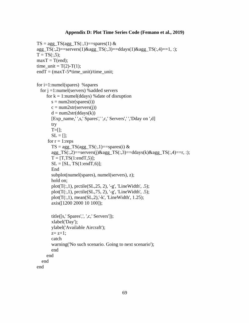
69

Appendix D: Plot Time Series Code (Femano et al., 2019)

TS = agg_TS(agg_TS(:,1)==spares(1) & agg_TS(:,2)==servers(1)&agg_TS(:,3)==ddays(1)&agg_TS(:,4)==1, :); T = TS(:,5); maxT = T(end); time_unit = T(2)-T(1); endT = (maxT-5*time_unit)/time_unit; for i=1:numel(spares) %spares for j =1:numel(servers) %added servers for k = 1:numel(ddays) %date of disruption s = num2str(spares(i)) c = num2str(servers(j)) d = num2str(ddays(k)) [Exp_name,' ',s,' Spares',' ',c,' Servers',' ','Dday on ',d] try T=[]; SL = []; for r = 1:reps

TS = agg_TS(agg_TS(:,1)==spares(i) & agg_TS(:,2)==servers(j)&agg_TS(:,3)==ddays(k)&agg_TS(:,4)==r, :); T = [T,TS(1:endT,5)]; SL = [SL, TS(1:endT,6)];

End subplot(numel(spares), numel(servers), z);

hold on; plot(T(:,1), prctile(SL,25, 2), '-g', 'LineWidth', .5); plot(T(:,1), prctile(SL,75, 2), '-g', 'LineWidth', .5); plot(T(:,1), mean(SL,2),'-k', 'LineWidth', 1.25); axis([1200 2000 10 100]); title([s,' Spares',', ',c,' Servers']); xlabel('Day'); ylabel('Available Aircraft'); z= z+1; catch warning('No such scenario. Going to next scenario'); end end end end

70

Bibliography

Bakshi, N. & Kleindorfer, P. R. (2009). Co-opetition and investment for supply-chain

resilience. Production and Operations Management, 18(6), 583-603.

https://doi.org/10.1111/j.1937-5956.2009.01031.x.

Blackhurst. J, Craighead, C. W., Elkins, D., & Handfield, R. B. (2005). An empirically

derived agenda of critical research issues for managing supply-chain disruptions.

International Journal of Production Research, 43(19), 4067-4081.

https://doi.org/10.1080/00207540500151549.

Bonferroni Correction. (2019). Statistics Solutions: Advancement through Clarity.

Retrieved February 19, 2020 from

https://www.statisticssolutions.com/bonferroni-correction/

Carter, C. R. & Rogers, D. S. (2008). A framework of sustainable supply chain

management: moving toward new theory. International Journal of Physical

Distribution & Logistics Management, 38(5), 360-387.

https://doi.org/10.1108/09600030810882816.

Carvalho, H., Barroso, A. P., Machado, V. H., Azevedo, S., & Cruz-Machado, V. (2012).

Supply chain redesign for resilience using simulation. Computers & Industrial

Engineering, 62(1), 329-341. https://doi.org/10.1016/j.cie.2011.10.003.

Chopra, S., & Sodhi, M. S. (2004). Managing risk to avoid supply-chain breakdown. MIT

Sloan Management Review, 46(1), 53-62. Retrieved from

https://sloanreview.mit.edu/article/managing-risk-to-avoid-supplychain-breakdown/.

https://doi.org/10.1111/j.1937-5956.2009.01031.x

https://doi.org/10.1080/00207540500151549

https://doi.org/10.1108/09600030810882816

https://doi.org/10.1016/j.cie.2011.10.003

71

Christopher, M. & Peck, H. (2004). Building the resilient supply chain. The International

Journal of Logistics Management, 15(2), 1-14.

https://doi.org/10.1108/09574090410700275.

Craighead, C. W., Blackhurst, J., Rungtusanatham, M. J., & Handfield, R. B. (2007). The

severity of supply chain disruptions: design characteristics and mitigation capabilities.

Decision Sciences, 38(1), 131-156.

https://doi.org/10.1111/j.1540-5915.2007.00151.x.

de Neufville, R., & Scholtes, S. (2011). Flexibility in Engineering Design. Cambridge,

MA: The MIT Press.

Directorate of Engineering Support. (2007). Historical Air Force Construction Cost

Handbook. Retrieved from https://wbdg.org/FFC/AF/AFH/histbook.pdf.

Femano, A. L., Shannon, Z. B., Breitbach, T. W., & Steeneck, D. W. (2019). Tradeoff

between investments in inventory and production capability in supply chains prone to

disruption. Unpublished Manuscript.

Forbes, S. L. & Wilson, M. M. J. (2018). Resilience and response of wine supply chains

to disaster: the Christchurch earthquake sequence. The International Review of Retail,

Distribution, and Consumer Research, 28(5), 472-489.

https://doi.org/10.1080/09593969.2018.1500931.

Graves, S. C. & Tomlin, B. T. (2003). Process flexibility in supply chains. Management

Science, 49(7), 907-919. https://doi.org/10.1287/mnsc.49.7.907.16381.

Ivanov, D. (2018). Revealing interfaces of supply chain resilience and sustainability: a

simulation study. International Journal of Production Research, 56(10), 3507-3523.

https://doi.org/10.1080/00207543.2017.1343507.

https://doi.org/10.1108/09574090410700275

https://doi.org/10.1287/mnsc.49.7.907.16381

https://doi.org/10.1080/00207543.2017.1343507

72

Ivanov, D., Sokolov, B., & Dolgui, A. (2014). The ripple effect in supply chains: trade-

off ‘efficiency-flexibility-resilience’ in disruption management. International Journal

of Production Research, 52(7), 2154-2172.

https://doi.org/10.1080/00207543.2013.858836.

Jordan, W. C. & Graves, S. C. (1995). Principles on the benefits of manufacturing

process flexibility. Management Science, 41(4), 577-594.

https://doi.org/10.1287/mnsc.41.4.577.

Kleindorfer, P. R. & Saad, G. H. (2005). Managing disruption risks in supply chains.

Production and Operations Management, 14(1), 53-68.

https://doi.org/10.1111/j.1937-5956.2005.tb00009.x.

Liu, F., Song, J., & Tong, J. D. (2016). Building supply chain resilience through virtual

stockpile pooling. Production and Operations Management, 25(10), 1745-1762.

https://doi.org/10.1111/poms.12573.

Lücker, F., Seifert, R. W., & Işık, B. (2019). Roles of inventory and reserve capacity in

mitigating supply chain disruption risk. International Journal of Production

Research, 57(4), 1238-1249. https://doi.org/10.1080/00207543.2018.1504173.

Melnyk, S. A., Zobel, C. W., Macdonald, J. R., & Griffis, S. E. (2013). Making sense of

transient responses in simulation studies. International Journal of Production

Research, 52(3), 617-632. https://doi.org/10.1080/00207543.2013.803626.

Milton, J. S. & Arnold, J. C. (2003). Introduction to Probability and Statistics: Principles

and Applications for Engineering and the Computing Sciences. (4th Edition). McGraw

Hill Education.

https://doi.org/10.1080/00207543.2013.858836

https://doi.org/10.1111/poms.12573

https://doi.org/10.1080/00207543.2018.1504173

https://doi.org/10.1080/00207543.2013.803626

73

Otani, A. (2020, January). Outbreak tests investors’ bets on global recovery. The Wall

Street Journal, pp. B1, B12.

Petcoff, R. P. (2010, May 5). Air Force program recognized for excellence in

government. U.S Air Force. Retrieved from

https://www.af.mil/News/Article-Display/Article/116767/air-force-program-

recognized-for-excellence-in-government/

Pettit, T. J., Fiksel, J., & Croxton, K. L. (2010). Ensuring supply chain resilience:

development of a conceptual framework. Journal of Business Logistics, 31(1), 1-21.

https://doi.org/10.1002/j.2158-1592.2010.tb00125.x.

Repair Network Integration Office, Air Force material Command Directorate of

Logistics, & Civil Engineering and Force Protection. (2016). Repair Network

Integration helps build a better repair network. Retrieved from

https://www.af.mil/News/Article-Display/Article/902309/repair-network-integration-

helps-build-a-better-repair-network/.

Saghafian, S., & Van Oyen., M. P. (2011). The value of flexible backup suppliers and

disruption risk information: newsvendor analysis with recourse. IIE Transactions,

44(10), 834-867. https://doi.org/10.1080/0740817X.2012.654846.

Saghafian, S., & Van Oyen., M. P. (2016). Compensating for dynamic supply chain

disruptions: backup flexibility design. Operations Research, 64(2), 390-405.

https://doi.org/10.1287/opre.2016.1478.

Schmitt, A. J. & Singh, M. (2012). A quantitative analysis of disruption risk in a multi-

echelon supply chain. International Journal of Production Economics, 139(1), 22-32.

https://doi.org/10.1016/j.ijpe.2012.01.004.

https://doi.org/10.1002/j.2158-1592.2010.tb00125.x

https://doi.org/10.1080/0740817X.2012.654846

https://doi.org/10.1287/opre.2016.1478

https://doi.org/10.1016/j.ijpe.2012.01.004

74

Sheffi, Y. & Rice Jr. J. B. (2005). A supply chain view of the resilient enterprise. MIT

Sloan Management Review, 47(1), 41-48. Retrieved from

https://www.researchgate.net/publication/255599289_A_Supply_Chain_View_of_the

_Resilient_Enterprise.

Sheffi, Y. (2001). Supply chain management under the threat of international terrorism.

International Journal of Logistics Management,12(2), 1-11.

https://doi.org/10.1108/09574090110806262. Simchi-Levi, D. & Wei, Y. (2012). Understanding the performance of the long chain and

sparse designs in process flexibility. Operations Research, 60(5), 1125-1141.

https://doi.org/10.1287/opre.1120.1081.

Sleptchenko, A., van der Heijden, M. C., & van Harten, A. (2003). Trade-off between

inventory and repair capacity in spare part networks. Journal of Operational

Research Society, 54(3), 263-272. https://doi.org/10.1057/palgrave.jors.2601511.

Snyder, L. V., Atan, Z., Peng, P., Rong, Y., Schmitt, A. J., & Sinsoysal, B. (2012).

OR/MS models for supply chain disruptions: A review. IIE Transactions, 48(2), 89-

109. https://doi.org/10.1080/0740817X.2015.1067735.

Tang, C. S. & Tomlin, B. T. (2008). The power of process flexibility for mitigating

supply chain risks. International Journal of Production Economics, 116(1), 12-27.

https://doi.org/10.1016/j.ijpe.2008.07.008.

Tang, C. S. (2006). Robust strategies for mitigating supply chain disruptions.

International Journal of Logistics: Research and Applications, 9(1), 33-45.

https://doi.org/10.1080/13675560500405584.

https://doi.org/10.1057/palgrave.jors.2601511

https://doi.org/10.1080/0740817X.2015.1067735

https://doi.org/10.1016/j.ijpe.2008.07.008

https://doi.org/10.1080/13675560500405584

75

Tomlin, B. (2006). On the value of mitigation and contingency strategies for managing

supply chain disruption risks. Management Science, 52(5), 639-657.

https://doi.org/10.1287/mnsc.1060.0515

Tripp, R. S., McGarvey, R. G., Van Roo, B. D., Masters, J. M., & Sollinger, J. M. (2010).

A repair network concept for air force maintenance. RAND Corporation. Retrieved

from

https://www.rand.org/content/dam/rand/pubs/monographs/2010/RAND_MG919.pdf

Tukamuhabwa, B. R., Stevenson, M., Busby, J., Zorzini, M. (2015). Supply chain

resilience: definition, review and theoretical foundations for further study.

International Journal of Production Research, 53(18), 5592-5623.

http://dx.doi.org/10.1080/00207543.2015.1037934

Wang, D. & Ip, W. H. (2009). Evaluation and analysis of logistic network resilience with

application to aircraft servicing. IEEE Systems Journal, 3(2), 166-172.

https://doi.org/10.1109/JSYST.2009.2017395.

Yang, Z., Aydin, G., Babich, V., & Beil, D. R. (2009). Supply disruptions, asymmetric

information, and a backup production option. Management Science, 52(2), 192-209.

https://doi.org/10.1287//mnsc.1080.0943.

https://doi.org/10.1287/mnsc.1060.0515

76

REPORT DOCUMENTATION PAGE Form Approved OMB No. 074-0188

The public reporting burden for this collection of information is estimated to average 1 hour per response, including the time for reviewing instructions, searching existing data sources, gathering and maintaining the data needed, and completing and reviewing the collection of information. Send comments regarding this burden estimate or any other aspect of the collection of information, including suggestions for reducing this burden to Department of Defense, Washington Headquarters Services, Directorate for Information Operations and Reports (0704-0188), 1215 Jefferson Davis Highway, Suite 1204, Arlington, VA 22202-4302. Respondents should be aware that notwithstanding any other provision of law, no person shall be subject to an penalty for failing to comply with a collection of information if it does not display a currently valid OMB control number. PLEASE DO NOT RETURN YOUR FORM TO THE ABOVE ADDRESS. 1. REPORT DATE (DD-MM-YYYY)

26-03-2020 2. REPORT TYPE

Master’s Thesis 3. DATES COVERED (From – To)

January 2019 – March 2020

TITLE AND SUBTITLE

Resilient Aircraft Sustainment: Quantifying Resilience through Asset and Capacity Allocation

5a. CONTRACT NUMBER

5b. GRANT NUMBER 5c. PROGRAM ELEMENT NUMBER

6. AUTHOR(S)

Shannon, Zachary, B

5d. PROJECT NUMBER

5e. TASK NUMBER

5f. WORK UNIT NUMBER

7. PERFORMING ORGANIZATION NAMES(S) AND ADDRESS(S) Air Force Institute of Technology Graduate School of Engineering and Management (AFIT/EN) 2950 Hobson Way, Building 640 WPAFB OH 45433-7765

8. PERFORMING ORGANIZATION REPORT NUMBER AFIT-ENS-MS-20-M-288

9. SPONSORING/MONITORING AGENCY NAME(S) AND ADDRESS(ES) Intentionally left blank

10. SPONSOR/MONITOR’S ACRONYM(S)

11. SPONSOR/MONITOR’S REPORT NUMBER(S)

12. DISTRIBUTION/AVAILABILITY STATEMENT DISTRUBTION STATEMENT A. APPROVED FOR PUBLIC RELEASE; DISTRIBUTION UNLIMITED.

13. SUPPLEMENTARY NOTES This material is declared a work of the U.S. Government and is not subject to copyright protection in the United States.

14. ABSTRACT Decision makers lack a clear, generalizable method to quantify how additional investment in inventory and capacity equates to additional levels of resilience. This research facilitates a deeper understanding of the intricacies and complex interconnectedness of organizational supply chains by monetarily quantifying changes in network resilience. The developed Area under the Curve metric (AUC) is used to quantify the level of demand that each asset allocation can meet during a disruptive event. Due to its applicability across multiple domains, the USAF F-16 repair network in the Pacific theater (PACAF) is modeled utilizing discrete event simulation and used as the illustrating example. This research uses various levels of production capacity and response time as the primary resilience levers. However, it is essential to simultaneously invest in inventory and capacity to realize the greatest impacts on resilience. Real-world demand and cost data are incorporated to identify the inherent cost-resilience relationships, essential for evaluating the response and recovery capabilities across the developed scenarios. Results indicate that recovery capacity and response time are the greatest drivers of recovery after a disruption. Additionally, numerous network designs employing various levels of design flexibility are evaluated and recommended for future capacity expansion.

15. SUBJECT TERMS Discrete-Event Simulation, Supply Chain Resilience, Network Disruption, Quantifying Resilience 16. SECURITY CLASSIFICATION OF:

17. LIMITATION OF ABSTRACT

UU

18. NUMBER OF PAGES

86

19a. NAME OF RESPONSIBLE PERSON Maj Timothy Breitbach, AFIT/ENS

a. REPORT

U

b. ABSTRACT

U

c. THIS PAGE

U

19b. TELEPHONE NUMBER (Include area code) (937) 255-3636 x4458 [email protected]

Standard Form 298 (Rev. 8-98) Prescribed by ANSI Std. Z39-18

Documents

Resilient Aircraft Sustainment: Quantifying Resilience